using simple sdes (stochastic differential equations - math nist
TRANSCRIPT

A Little History on Monte Carlo Methods for PDEsThe Feynman-Kac Formula and SDEs
Some Examples Using This for Computing Elliptic ProblemsHyperbolic equations: the telegrapher’s equation & an application
Conclusions and open problems
Using Simple SDEs (Stochastic DifferentialEquations) to Solve Complicated PDEs (Partial
Differential Equations)
Prof. Michael Mascagni
Department of Computer Science & School of Computational ScienceFlorida State University, Tallahassee, FL 32306 USA
E-mail: [email protected] or [email protected]: http://www.cs.fsu.edu/∼mascagni
With help from Drs. James Given, Chi-Ok Hwang, Aneta Karaivanova and NikolaiSimonov
Research supported by ARO, DOE/ASCI, NATO, and NSF
Prof. Michael Mascagni Simple SDEs for PDEs

A Little History on Monte Carlo Methods for PDEsThe Feynman-Kac Formula and SDEs
Some Examples Using This for Computing Elliptic ProblemsHyperbolic equations: the telegrapher’s equation & an application
Conclusions and open problems
Outline of the Talk
1 A Little History on Monte Carlo Methods for PDEs
2 The Feynman-Kac Formula and SDEsFor Elliptic EquationsFor Parabolic Equations
3 Some Examples Using This for Computing Elliptic ProblemsProblems in electrostatics/materialsVarious acceleration techniques for elliptic PDEs
4 Hyperbolic equations: the telegrapher’s equation & anapplication
5 Conclusions and open problems
Prof. Michael Mascagni Simple SDEs for PDEs

A Little History on Monte Carlo Methods for PDEsThe Feynman-Kac Formula and SDEs
Some Examples Using This for Computing Elliptic ProblemsHyperbolic equations: the telegrapher’s equation & an application
Conclusions and open problems
Early History of MCMs for PDEs
1 Courant, Friedrichs, and Lewy: Their pivotal 1928 paperhas probabilistic interpretations and MC algorithms forlinear elliptic and parabolic problems
2 Fermi/Ulam/von Neumann: Atomic bomb calculations weredone using Monte Carlo methods for neutron transport,their success inspired much post-War work especially innuclear reactor design
3 Kac and Donsker: Used large deviation calculations toestimate eigenvalues of a linear Schrödinger equation
4 Forsythe and Leibler: Derived a MCM for solving speciallinear systems related to discrete elliptic PDE problems
Prof. Michael Mascagni Simple SDEs for PDEs

A Little History on Monte Carlo Methods for PDEsThe Feynman-Kac Formula and SDEs
Some Examples Using This for Computing Elliptic ProblemsHyperbolic equations: the telegrapher’s equation & an application
Conclusions and open problems
Early History of MCMs for PDEs
5 Curtiss: Compared Monte Carlo, direct and iterativesolution methods for Ax = b
General conclusions of all this work (as other methods wereexplored) is that random walk methods do worse thanconventional methods on serial computers except whenmodest precision and few solution values are requiredMuch of this “conventional wisdom” needs revision due tocomplexity differences with parallel implementations
6 Muller & Curtiss: Monte Carlo methods for elliptic PDEs
Prof. Michael Mascagni Simple SDEs for PDEs

A Little History on Monte Carlo Methods for PDEsThe Feynman-Kac Formula and SDEs
Some Examples Using This for Computing Elliptic ProblemsHyperbolic equations: the telegrapher’s equation & an application
Conclusions and open problems
For Elliptic EquationsFor Parabolic Equations
Elliptic PDEs as Boundary Value Problems1 Elliptic PDEs describe equilibrium, like the electrostatic
field set up by a charge distribution, or the strain in a beamdue to loading
2 No time dependence in elliptic problems so it is natural tohave the interior configuration satisfy a PDE with boundaryconditions to choose a particular global solution
3 Elliptic PDEs are thus part of boundary value problems(BVPs) such as the famous Dirichlet problem for Laplace’sequation:
12∆u(x) = 0, x ∈ Ω, u(x) = f (x), x ∈ ∂Ω (2.1)
4 Here Ω ⊂ Rs is a open set (domain) with a smoothboundary ∂Ω and f (x) is the given boundary condition
Prof. Michael Mascagni Simple SDEs for PDEs

A Little History on Monte Carlo Methods for PDEsThe Feynman-Kac Formula and SDEs
Some Examples Using This for Computing Elliptic ProblemsHyperbolic equations: the telegrapher’s equation & an application
Conclusions and open problems
For Elliptic EquationsFor Parabolic Equations
Probabilistic Approaches to Elliptic PDEs
Early this century probabilists placed measures ondifferent sets including sets of continuous functionsA. Called Wiener measureB. Gaussian based: 1√
2πte−
x22t
C. Sample paths are Brownian motionD. Related to linear PDEs
E.g. u(x) = Ex [f (X x(t∂Ω))] is the Wiener integralrepresentation of the solution to (2.1), to prove it we mustcheck:A. u(x) = f (x) on ∂ΩB. u(x) has the MVP
Interpretation via Brownian motion and/or aprobabilistic Green’s function
Prof. Michael Mascagni Simple SDEs for PDEs

A Little History on Monte Carlo Methods for PDEsThe Feynman-Kac Formula and SDEs
Some Examples Using This for Computing Elliptic ProblemsHyperbolic equations: the telegrapher’s equation & an application
Conclusions and open problems
For Elliptic EquationsFor Parabolic Equations
Probabilistic Approaches to Elliptic PDEs
Important: t∂Ω = first passage (hitting) time of the pathX x(·) started at x to ∂Ω, statistics based on this randomvariable are intimately related to elliptic problemsCan generalize Wiener integrals to different BVPs via therelationship between elliptic operators, stochasticdifferential equations (SDEs), and the Feynman-Kacformula
Prof. Michael Mascagni Simple SDEs for PDEs

A Little History on Monte Carlo Methods for PDEsThe Feynman-Kac Formula and SDEs
Some Examples Using This for Computing Elliptic ProblemsHyperbolic equations: the telegrapher’s equation & an application
Conclusions and open problems
For Elliptic EquationsFor Parabolic Equations
Probabilistic Approaches to Elliptic PDEs
x; starting point
zfirst passage location
Prof. Michael Mascagni Simple SDEs for PDEs

A Little History on Monte Carlo Methods for PDEsThe Feynman-Kac Formula and SDEs
Some Examples Using This for Computing Elliptic ProblemsHyperbolic equations: the telegrapher’s equation & an application
Conclusions and open problems
For Elliptic EquationsFor Parabolic Equations
Probabilistic Approaches to Elliptic PDEs
E.g. consider the general elliptic PDE:
Lu(x)− c(x)u(x) = g(x), x ∈ Ω, c(x) ≥ 0,
u(x) = f (x), x ∈ ∂Ω (1.1a)
where L is an elliptic partial differential operator of theform:
L =12
s∑i,j=1
aij(x)∂2
∂xi∂xj+
s∑i=1
bi(x)∂
∂xi, (1.1b)
Prof. Michael Mascagni Simple SDEs for PDEs

A Little History on Monte Carlo Methods for PDEsThe Feynman-Kac Formula and SDEs
Some Examples Using This for Computing Elliptic ProblemsHyperbolic equations: the telegrapher’s equation & an application
Conclusions and open problems
For Elliptic EquationsFor Parabolic Equations
Probabilistic Approaches to Elliptic PDEs
The Wiener integral representation is:
u(x) = ELx
[ ∫ t∂Ω
0
f (X x(t∂Ω))
t∂Ω− g(X x(t))
e−
R t0 c(X x(s)) ds dt
](1.2a)
the expectation is w.r.t. paths which are solutions to thefollowing (vector) SDE:
dX x(t) = σ(X x(t)) dW (t) + b(X x(t)) dt , X x(0) = x (1.2b)
Prof. Michael Mascagni Simple SDEs for PDEs

A Little History on Monte Carlo Methods for PDEsThe Feynman-Kac Formula and SDEs
Some Examples Using This for Computing Elliptic ProblemsHyperbolic equations: the telegrapher’s equation & an application
Conclusions and open problems
For Elliptic EquationsFor Parabolic Equations
Probabilistic Approaches to Elliptic PDEs
The matrix σ(·) is the Choleski factor (matrix-like squareroot) of aij(·) in (1.1b)To use these ideas to construct MCMs for elliptic BVPs onemust:A. Simulate sample paths via SDEs (1.2b)B. Evaluate (1.2a) on the sample pathsC. Sample until variance is acceptable
Prof. Michael Mascagni Simple SDEs for PDEs

A Little History on Monte Carlo Methods for PDEsThe Feynman-Kac Formula and SDEs
Some Examples Using This for Computing Elliptic ProblemsHyperbolic equations: the telegrapher’s equation & an application
Conclusions and open problems
For Elliptic EquationsFor Parabolic Equations
Different SDEs, Different Processes, DifferentEquations
The SDE gives us a process, and the process defines L(note: a complete definition of L includes the boundaryconditions)We have solved only the Dirichlet problem, what aboutother BCs?Neumann Boundary Conditions: ∂u
∂n = g(x) on ∂Ω
If one uses reflecting Brownian motion, can sample overthese pathsMixed Boundary Conditions: α∂u
∂n + βu = g(x) on ∂Ω
Use reflecting Brownian motion and first passageprobabilities, togetherIn some simple cases, only X x(t∂Ω)) is needed
Prof. Michael Mascagni Simple SDEs for PDEs

A Little History on Monte Carlo Methods for PDEsThe Feynman-Kac Formula and SDEs
Some Examples Using This for Computing Elliptic ProblemsHyperbolic equations: the telegrapher’s equation & an application
Conclusions and open problems
For Elliptic EquationsFor Parabolic Equations
Probabilistic Approaches to Parabolic PDEs viaFeynman-Kac
Can generalize Wiener integrals to a wide class of IBVPsvia the relationship between elliptic operators, stochasticdifferential equations (SDEs), and the Feynman-KacformulaRecall that t →∞ parabolic → elliptic
Prof. Michael Mascagni Simple SDEs for PDEs
A Little History on Monte Carlo Methods for PDEsThe Feynman-Kac Formula and SDEs
Some Examples Using This for Computing Elliptic ProblemsHyperbolic equations: the telegrapher’s equation & an application
Conclusions and open problems
For Elliptic EquationsFor Parabolic Equations
Probabilistic Approaches to Parabolic PDEs viaFeynman-Kac
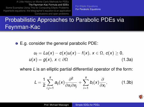
E.g. consider the general parabolic PDE:
ut = Lu(x)− c(x)u(x)− f (x), x ∈ Ω, c(x) ≥ 0,
u(x) = g(x), x ∈ ∂Ω (1.3a)
where L is an elliptic partial differential operator of the form:
L =12
s∑i,j=1
aij(x)∂2
∂xi∂xj+
s∑i=1
bi(x)∂
∂xi, (1.3b)
Prof. Michael Mascagni Simple SDEs for PDEs

A Little History on Monte Carlo Methods for PDEsThe Feynman-Kac Formula and SDEs
Some Examples Using This for Computing Elliptic ProblemsHyperbolic equations: the telegrapher’s equation & an application
Conclusions and open problems
For Elliptic EquationsFor Parabolic Equations
Probabilistic Approaches to Parabolic PDEs viaFeynman-Kac
The Wiener integral representation is:
u(x , t) = ELx
[g(X x(τ∂Ω))−
∫ t
0f (X x(t))e−
R t0 c(X x(s)) ds dt
](1.4a)
the expectation is w.r.t. paths which are solutions to thefollowing (vector) SDE:
dX x(t) = σ(X x(t)) dW (t) + b(X x(t)) dt , X x(0) = x (1.4b)
The matrix σ(·) is the Choleski factor (matrix-like squareroot) of aij(·) in (1.3b)
Prof. Michael Mascagni Simple SDEs for PDEs

A Little History on Monte Carlo Methods for PDEsThe Feynman-Kac Formula and SDEs
Some Examples Using This for Computing Elliptic ProblemsHyperbolic equations: the telegrapher’s equation & an application
Conclusions and open problems
Problems in electrostatics/materialsVarious acceleration techniques for elliptic PDEs
The First Passage (FP) Probability is the Green’sFunction
Back to our canonical elliptic boundary value problem:
12∆u(x) = 0, x ∈ Ω
u(x) = f (x), x ∈ ∂Ω
Distribution of z is uniform on the sphereMean of the values of u(z) over the sphere is u(x)
u(x) has mean-value property and harmonicAlso, u(x) satisfies the boundary condition
u(x) = Ex [f (X x(t∂Ω))] (3.1)
Prof. Michael Mascagni Simple SDEs for PDEs

A Little History on Monte Carlo Methods for PDEsThe Feynman-Kac Formula and SDEs
Some Examples Using This for Computing Elliptic ProblemsHyperbolic equations: the telegrapher’s equation & an application
Conclusions and open problems
Problems in electrostatics/materialsVarious acceleration techniques for elliptic PDEs
The First Passage (FP) Probability is the Green’sFunction
Reinterpreting as an average of the boundary values
u(x) =
∫∂Ω
p(x , y)f (y) dy (3.2)
Another representation in terms of an integral over theboundary
u(x) =
∫∂Ω
∂g(x , y)
∂nf (y) dy (3.3)
g(x , y) – Green’s function of the Dirichlet problem in Ω
=⇒ p(x , y) =∂g(x , y)
∂n(3.4)
Prof. Michael Mascagni Simple SDEs for PDEs

A Little History on Monte Carlo Methods for PDEsThe Feynman-Kac Formula and SDEs
Some Examples Using This for Computing Elliptic ProblemsHyperbolic equations: the telegrapher’s equation & an application
Conclusions and open problems
Problems in electrostatics/materialsVarious acceleration techniques for elliptic PDEs
‘Walk on Spheres’ (WOS) and ‘Green’s Function FirstPassage’ (GFFP) Algorithms
Green’s function is known=⇒ direct simulation of exit points and computation of thesolution through averaging boundary valuesGreen’s function is unknown=⇒ simulation of exit points from standard subdomains ofΩ, e.g. spheres=⇒ Markov chain of ‘Walk on Spheres’ (or GFFPalgorithm) x0 = x , x1, . . . , xNxi → ∂Ω and hits ε-shell is N = O(| ln(ε)|) stepsxN simulates exit point from Ω with O(ε) accuracy
Prof. Michael Mascagni Simple SDEs for PDEs

A Little History on Monte Carlo Methods for PDEsThe Feynman-Kac Formula and SDEs
Some Examples Using This for Computing Elliptic ProblemsHyperbolic equations: the telegrapher’s equation & an application
Conclusions and open problems
Problems in electrostatics/materialsVarious acceleration techniques for elliptic PDEs
‘Walk on Spheres’ (WOS) and ‘Green’s Function FirstPassage’ (GFFP) Algorithms
WOS:
Prof. Michael Mascagni Simple SDEs for PDEs

A Little History on Monte Carlo Methods for PDEsThe Feynman-Kac Formula and SDEs
Some Examples Using This for Computing Elliptic ProblemsHyperbolic equations: the telegrapher’s equation & an application
Conclusions and open problems
Problems in electrostatics/materialsVarious acceleration techniques for elliptic PDEs
Timing with WOS
Prof. Michael Mascagni Simple SDEs for PDEs

A Little History on Monte Carlo Methods for PDEsThe Feynman-Kac Formula and SDEs
Some Examples Using This for Computing Elliptic ProblemsHyperbolic equations: the telegrapher’s equation & an application
Conclusions and open problems
Problems in electrostatics/materialsVarious acceleration techniques for elliptic PDEs
Solc-Stockmayer Model without Potential
Prof. Michael Mascagni Simple SDEs for PDEs

A Little History on Monte Carlo Methods for PDEsThe Feynman-Kac Formula and SDEs
Some Examples Using This for Computing Elliptic ProblemsHyperbolic equations: the telegrapher’s equation & an application
Conclusions and open problems
Problems in electrostatics/materialsVarious acceleration techniques for elliptic PDEs
The Simulation-Tabulation (S-T) Method forGeneralization
Green’s function for the non-intersected surface of asphere located on the surface of a reflecting sphere
Prof. Michael Mascagni Simple SDEs for PDEs

A Little History on Monte Carlo Methods for PDEsThe Feynman-Kac Formula and SDEs
Some Examples Using This for Computing Elliptic ProblemsHyperbolic equations: the telegrapher’s equation & an application
Conclusions and open problems
Problems in electrostatics/materialsVarious acceleration techniques for elliptic PDEs
Another S-T Application: Mean Trapping Rate
In a domain of nonoverlapping spherical traps :
Prof. Michael Mascagni Simple SDEs for PDEs

A Little History on Monte Carlo Methods for PDEsThe Feynman-Kac Formula and SDEs
Some Examples Using This for Computing Elliptic ProblemsHyperbolic equations: the telegrapher’s equation & an application
Conclusions and open problems
Problems in electrostatics/materialsVarious acceleration techniques for elliptic PDEs
Porous Media: Complicated Interfaces
Prof. Michael Mascagni Simple SDEs for PDEs

A Little History on Monte Carlo Methods for PDEsThe Feynman-Kac Formula and SDEs
Some Examples Using This for Computing Elliptic ProblemsHyperbolic equations: the telegrapher’s equation & an application
Conclusions and open problems
Problems in electrostatics/materialsVarious acceleration techniques for elliptic PDEs
Computing Capacitance Probabilistically
Hubbard-Douglas: can compute permeability of nonskewobject via capacitanceRecall that C = Q
u , if we hold conductor (Ω)at unit potentialu = 1, then C = total charge on conductor (surface)The PDE system for the potential is
∆u = 0, x /∈ Ω; u = 1, x ∈ ∂Ω; u → 0 as x →∞(3.5)
Recall u(x) = Ex [f (X x(t∂Ω))] = probability of walkerstarting at x hitting Ω before escaping to infinityCharge density is first passage probabilityCapacitance (relative to a sphere) is probability of walkerstarting at x (random chosen on sphere) hitting Ω beforeescaping to infinity
Prof. Michael Mascagni Simple SDEs for PDEs

A Little History on Monte Carlo Methods for PDEsThe Feynman-Kac Formula and SDEs
Some Examples Using This for Computing Elliptic ProblemsHyperbolic equations: the telegrapher’s equation & an application
Conclusions and open problems
Problems in electrostatics/materialsVarious acceleration techniques for elliptic PDEs
Various Laplacian Green’s Functions for Green’sFunction First Passage (GFFP)
OO
O
Putting back (a) Void space(b) Intersecting(c)
Prof. Michael Mascagni Simple SDEs for PDEs

A Little History on Monte Carlo Methods for PDEsThe Feynman-Kac Formula and SDEs
Some Examples Using This for Computing Elliptic ProblemsHyperbolic equations: the telegrapher’s equation & an application
Conclusions and open problems
Problems in electrostatics/materialsVarious acceleration techniques for elliptic PDEs
Escape to ∞ in A Single Step
Probability that a diffusing particle at r0 > b will escape toinfinity
Pesc = 1− br0
= 1− α (3.6)
Putting-back distribution density function
ω(θ, φ) =1− α2
4π[1− 2α cos θ + α2]3/2 (3.7)
(b, θ, φ) ; spherical coordinates of the new position whenthe old position is put on the polar axis
Prof. Michael Mascagni Simple SDEs for PDEs

A Little History on Monte Carlo Methods for PDEsThe Feynman-Kac Formula and SDEs
Some Examples Using This for Computing Elliptic ProblemsHyperbolic equations: the telegrapher’s equation & an application
Conclusions and open problems
Problems in electrostatics/materialsVarious acceleration techniques for elliptic PDEs
Charge Density on a Circular Disk via Last-Passage
Prof. Michael Mascagni Simple SDEs for PDEs

A Little History on Monte Carlo Methods for PDEsThe Feynman-Kac Formula and SDEs
Some Examples Using This for Computing Elliptic ProblemsHyperbolic equations: the telegrapher’s equation & an application
Conclusions and open problems
Problems in electrostatics/materialsVarious acceleration techniques for elliptic PDEs
Time Reversal Brownian Motion: Approach from theOutside
Prof. Michael Mascagni Simple SDEs for PDEs

A Little History on Monte Carlo Methods for PDEsThe Feynman-Kac Formula and SDEs
Some Examples Using This for Computing Elliptic ProblemsHyperbolic equations: the telegrapher’s equation & an application
Conclusions and open problems
Problems in electrostatics/materialsVarious acceleration techniques for elliptic PDEs
Approach from the Outside
P(x): prob. of diffusing from ε above lower FP surface to ∞
P(x) =
∫∂Ωy
g(x , y , ε)p(y ,∞)dS (3.8)
σ(x) = − 14π
ddε
∣∣∣∣∣ε=0
φ(x) =1
4π
ddε
∣∣∣∣∣ε=0
P(x) (3.9)
σ(x) =1
4π
∫∂Ωy
G(x , y)p(y ,∞)dS (3.10)
where
G(x , y) =ddε
∣∣∣∣∣ε=0
g(x , y , ε) (3.11)
G(x , y) satisfies a point dipole problem
Prof. Michael Mascagni Simple SDEs for PDEs

A Little History on Monte Carlo Methods for PDEsThe Feynman-Kac Formula and SDEs
Some Examples Using This for Computing Elliptic ProblemsHyperbolic equations: the telegrapher’s equation & an application
Conclusions and open problems
Problems in electrostatics/materialsVarious acceleration techniques for elliptic PDEs
Charge Density on the Circular Disk
G =34
cos θ
a3 (3.12)
σ(x) =3
16π
∫∂Ωr
cos θ
a3 p(r,∞)dS (3.13)
wherep(r,∞) = 1− 2
πarctan
√2b√
r2 − b2 +√
(r2 − b2)2 + 4b2x2
(3.14)
Prof. Michael Mascagni Simple SDEs for PDEs

A Little History on Monte Carlo Methods for PDEsThe Feynman-Kac Formula and SDEs
Some Examples Using This for Computing Elliptic ProblemsHyperbolic equations: the telegrapher’s equation & an application
Conclusions and open problems
Problems in electrostatics/materialsVarious acceleration techniques for elliptic PDEs
Charge Density on the Circular Disk
Prof. Michael Mascagni Simple SDEs for PDEs

A Little History on Monte Carlo Methods for PDEsThe Feynman-Kac Formula and SDEs
Some Examples Using This for Computing Elliptic ProblemsHyperbolic equations: the telegrapher’s equation & an application
Conclusions and open problems
Problems in electrostatics/materialsVarious acceleration techniques for elliptic PDEs
Edge Distribution on the Circular Disk
σ(r) =1
4π
1√1− r2
(3.15)
Let r = 1− x :σ(x) =
14π
1√2x
(1− x/2)−1/2 (3.16)
when x is small enough,σ(x) ' 1
4√
2π
1√x
(3.17)
σ(x) ' σe1√x
(3.18)
Prof. Michael Mascagni Simple SDEs for PDEs
A Little History on Monte Carlo Methods for PDEsThe Feynman-Kac Formula and SDEs
Some Examples Using This for Computing Elliptic ProblemsHyperbolic equations: the telegrapher’s equation & an application
Conclusions and open problems
Problems in electrostatics/materialsVarious acceleration techniques for elliptic PDEs
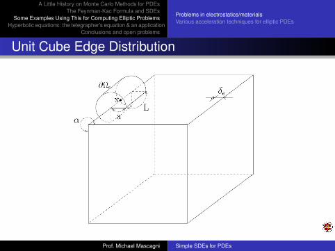
Unit Cube Edge Distribution
Prof. Michael Mascagni Simple SDEs for PDEs

A Little History on Monte Carlo Methods for PDEsThe Feynman-Kac Formula and SDEs
Some Examples Using This for Computing Elliptic ProblemsHyperbolic equations: the telegrapher’s equation & an application
Conclusions and open problems
Problems in electrostatics/materialsVarious acceleration techniques for elliptic PDEs
Unit Cube Edge Distribution
σ(x , δe) = δπ/α−1e σe(x) (3.19)
σ(x , δe): charge on a curve parallel to the edge separatedby δe
σe(x): edge distributionα: angle between the two intersecting surfaces, hereα = 3π/2
σe(x) =1
4πlim
δe→0δ
1−π/αe
∫∂Ωe
G(x , y)p(y ,∞)dS (3.20)
∂Ωe: cylindrical surface that intersects the pair ofabsorbing surfaces meeting at angle α
Prof. Michael Mascagni Simple SDEs for PDEs

A Little History on Monte Carlo Methods for PDEsThe Feynman-Kac Formula and SDEs
Some Examples Using This for Computing Elliptic ProblemsHyperbolic equations: the telegrapher’s equation & an application
Conclusions and open problems
Problems in electrostatics/materialsVarious acceleration techniques for elliptic PDEs
Unit Cube Edge Distribution
G(x , y):
G(x , y) =d
dδε
∣∣∣∣∣δε=0
g(x , y , δε) (3.21)
g(x , y , δε): Laplace Green’s function on the surface, ∂Ωe,with source point x at a distance δε from the absorbingsurface
p(y ,∞): probability that a diffusing particle, initiated atpoint y ∈ ∂Ωe, diffuses to infinity without returning to theabsorbing surface
Prof. Michael Mascagni Simple SDEs for PDEs

A Little History on Monte Carlo Methods for PDEsThe Feynman-Kac Formula and SDEs
Some Examples Using This for Computing Elliptic ProblemsHyperbolic equations: the telegrapher’s equation & an application
Conclusions and open problems
Problems in electrostatics/materialsVarious acceleration techniques for elliptic PDEs
Unit Cube Edge Distribution
G(ρ = a, φ, z) =1
Γ(5/3)22/34
9πLa
∞∑n=1
sin(2
3φ)
sin(nπz
L
)sin
(nπz ′
L
)×
(nπ
L
)2/3 1I2/3(
nπaL )
G(ρ, φ, z = 0) =1
Γ(5/3)22/34
9πL
∞∑n=1
sin(2
3φ)(nπ
L
)5/3sin
(nπz ′
L
)× 1
I2/3(nπa
L )
[I2/3
(nπaL
)K2/3
(nπρ
L
)− K2/3
(nπaL
)I2/3
(nπρ
L
)]
Prof. Michael Mascagni Simple SDEs for PDEs

A Little History on Monte Carlo Methods for PDEsThe Feynman-Kac Formula and SDEs
Some Examples Using This for Computing Elliptic ProblemsHyperbolic equations: the telegrapher’s equation & an application
Conclusions and open problems
Problems in electrostatics/materialsVarious acceleration techniques for elliptic PDEs
Unit Cube Edge Distribution
Figure: First- and last-passage edge computations
Prof. Michael Mascagni Simple SDEs for PDEs

A Little History on Monte Carlo Methods for PDEsThe Feynman-Kac Formula and SDEs
Some Examples Using This for Computing Elliptic ProblemsHyperbolic equations: the telegrapher’s equation & an application
Conclusions and open problems
Problems in electrostatics/materialsVarious acceleration techniques for elliptic PDEs
Unit Cube Edge Distribution
Figure: The slope, that is, the exponent of the edge distribution nearthe corner is approximately −0.20, that is, σe ∼ δ
−1/5c
Prof. Michael Mascagni Simple SDEs for PDEs

A Little History on Monte Carlo Methods for PDEsThe Feynman-Kac Formula and SDEs
Some Examples Using This for Computing Elliptic ProblemsHyperbolic equations: the telegrapher’s equation & an application
Conclusions and open problems
Problems in electrostatics/materialsVarious acceleration techniques for elliptic PDEs
Walk on the Boundary Algorithm
µ(y) = − 14π
∂φ
∂n(y) ; surface charge density
φ(x) =
∫∂Ω
1|x − y |
µ(y)dσ(y) ; electrostatic potential
Limit properties of the normal derivative (x → y outside of Ω):
µ(y) =
∫∂Ω
n(y) · (y − y ′)2π|y − y ′|3
µ(y ′)dσ(y ′)
By the ergodic theorem (convex Ω)∫∂Ω
v(y)π∞(y)dσ(y) = limN→∞
1N
N∑n=1
v(yn)
Prof. Michael Mascagni Simple SDEs for PDEs
A Little History on Monte Carlo Methods for PDEsThe Feynman-Kac Formula and SDEs
Some Examples Using This for Computing Elliptic ProblemsHyperbolic equations: the telegrapher’s equation & an application
Conclusions and open problems
Problems in electrostatics/materialsVarious acceleration techniques for elliptic PDEs
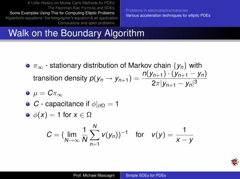
Walk on the Boundary Algorithm
π∞ - stationary distribution of Markov chain yn with
transition density p(yn → yn+1) =n(yn+1) · (yn+1 − yn)
2π|yn+1 − yn|3µ = Cπ∞
C - capacitance if φ|∂Ω = 1φ(x) = 1 for x ∈ Ω
C = ( limN→∞
1N
N∑n=1
v(yn))−1 for v(y) =
1x − y
Prof. Michael Mascagni Simple SDEs for PDEs

A Little History on Monte Carlo Methods for PDEsThe Feynman-Kac Formula and SDEs
Some Examples Using This for Computing Elliptic ProblemsHyperbolic equations: the telegrapher’s equation & an application
Conclusions and open problems
Problems in electrostatics/materialsVarious acceleration techniques for elliptic PDEs
Capacitance of the Unit Cube
Reitan-Higgins (1951) 0.6555Greenspan-Silverman (1965) 0.661
Cochran (1967) 0.6596Goto-Shi-Yoshida (1992) 0.6615897 ± 5 × 10⁻⁷
Conjectured Hubbard-Douglas (1993) 0.65946...Douglas-Zhou-Hubbard (1994) 0.6632 ± 0.0003Given-Hubbard-Douglas (1997) 0.660675 ± 0.00001
Read (1997) 0.6606785± 0.000003First passage method (2001) 0.660683± 0.000005
Walk on boundary algorithm (2002) 0.6606780± 0.0000004
Prof. Michael Mascagni Simple SDEs for PDEs

A Little History on Monte Carlo Methods for PDEsThe Feynman-Kac Formula and SDEs
Some Examples Using This for Computing Elliptic ProblemsHyperbolic equations: the telegrapher’s equation & an application
Conclusions and open problems
Problems in electrostatics/materialsVarious acceleration techniques for elliptic PDEs
Computing Protein Internal Energy
Poisson equation for the electrostatic potential inside amolecule G (a union of intersecting spherical atoms with:xm – centers, qm – charges)
−∇ε∇u(x) =M∑
m=1
qmδ(x − xm) , x ∈ G
Linearized Poisson-Boltzmann equation outside
∆u(x)− k2u(x) = 0 , x ∈ R3 \G
Continuity condition on the boundary
ui = ue , εi∂ui
∂n(y)= εe
∂ue
∂n(y), y ∈ ∂G
Prof. Michael Mascagni Simple SDEs for PDEs

A Little History on Monte Carlo Methods for PDEsThe Feynman-Kac Formula and SDEs
Some Examples Using This for Computing Elliptic ProblemsHyperbolic equations: the telegrapher’s equation & an application
Conclusions and open problems
Problems in electrostatics/materialsVarious acceleration techniques for elliptic PDEs
Computing Protein Internal Energy
Free energy of a molecule is defined as:
E =12
M∑m=1
u(0)(xm)qm ,
where u(0)(x) = u(x)− g(x) is the nonsingular part of theelectrostatic potential:
g(x) =M∑
m=1
qm
4πε
1|x − xm|
Prof. Michael Mascagni Simple SDEs for PDEs

A Little History on Monte Carlo Methods for PDEsThe Feynman-Kac Formula and SDEs
Some Examples Using This for Computing Elliptic ProblemsHyperbolic equations: the telegrapher’s equation & an application
Conclusions and open problems
Problems in electrostatics/materialsVarious acceleration techniques for elliptic PDEs
Computing Protein Internal Energy
Monte Carlo estimate for E : linear combination (functional) ofestimates for u(0)(xm).
ξ[E ] =12
M∑m=1
ξ[u(0)(xm)]qm , (3.22)
ξ[u(0)(xm)] = ξ[u(xNmm )]− g(xNm
m ) (3.23)
x0m = xm, x1
m, . . . , xNmm – Markov chain, every point x i
m is anexit point of the Brownian motion from the corresponding“atom" (Green’s function first passage)ym
1 = xNmm lies on the boundary, ∂G
Prof. Michael Mascagni Simple SDEs for PDEs
A Little History on Monte Carlo Methods for PDEsThe Feynman-Kac Formula and SDEs
Some Examples Using This for Computing Elliptic ProblemsHyperbolic equations: the telegrapher’s equation & an application
Conclusions and open problems
Problems in electrostatics/materialsVarious acceleration techniques for elliptic PDEs
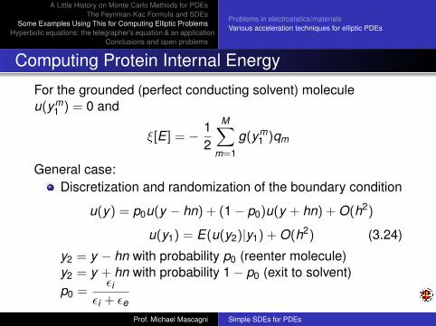
Computing Protein Internal Energy
For the grounded (perfect conducting solvent) moleculeu(ym
1 ) = 0 and
ξ[E ] = − 12
M∑m=1
g(ym1 )qm
General case:Discretization and randomization of the boundary condition
u(y) = p0u(y − hn) + (1− p0)u(y + hn) + O(h2)
u(y1) = E(u(y2)|y1) + O(h2) (3.24)
y2 = y − hn with probability p0 (reenter molecule)y2 = y + hn with probability 1− p0 (exit to solvent)p0 =
εi
εi + εe
Prof. Michael Mascagni Simple SDEs for PDEs

A Little History on Monte Carlo Methods for PDEsThe Feynman-Kac Formula and SDEs
Some Examples Using This for Computing Elliptic ProblemsHyperbolic equations: the telegrapher’s equation & an application
Conclusions and open problems
Problems in electrostatics/materialsVarious acceleration techniques for elliptic PDEs
Computing Protein Internal Energy
y2 inside: y3 ∈ ∂G is the last point of Markov chain (exit ofthe Brownian motion starting at y2)
u(y2) = E(u(y3)− g(y3) + g(y2)|y2) (3.25)
y2 outside: Walk on spheres algorithm (y2,0 = y2)y2,i+1 = y2,i + ω × di , di =distance(y2,i , ∂G)
Terminates with probabilitykdi
sinh(kdi)on every step, or
when dN < ε.y3 – the nearest to y2,N on the boundary
u(y2) = E(u(y3)|y2) + O(ε) (3.26)
Prof. Michael Mascagni Simple SDEs for PDEs

A Little History on Monte Carlo Methods for PDEsThe Feynman-Kac Formula and SDEs
Some Examples Using This for Computing Elliptic ProblemsHyperbolic equations: the telegrapher’s equation & an application
Conclusions and open problems
Problems in electrostatics/materialsVarious acceleration techniques for elliptic PDEs
Computing Protein Internal Energy
For ε = h2 relations (3.22), (3.23) and the recurrence (3.24),(3.25), (3.26) define an O(h)-biased Monte Carlo estimator.Mean number of steps in the algorithm is O(h−1 log(h) f (k)), fis a decreasing function.
Prof. Michael Mascagni Simple SDEs for PDEs

A Little History on Monte Carlo Methods for PDEsThe Feynman-Kac Formula and SDEs
Some Examples Using This for Computing Elliptic ProblemsHyperbolic equations: the telegrapher’s equation & an application
Conclusions and open problems
Problems in electrostatics/materialsVarious acceleration techniques for elliptic PDEs
Exit Points Using Walk on Subdomains
Figure: Exit points on the van der Waals surface of Barnase
Exit points on the van der Waals surface for the entire Barnasemolecule
Prof. Michael Mascagni Simple SDEs for PDEs

A Little History on Monte Carlo Methods for PDEsThe Feynman-Kac Formula and SDEs
Some Examples Using This for Computing Elliptic ProblemsHyperbolic equations: the telegrapher’s equation & an application
Conclusions and open problems
MCMs for Hyperbolic PDEs
We have constructed MCMs for both elliptic and parabolicPDEs but have not considered MCMs for hyperbolic PDEsexcept for Berger’s equation (was a very special case)In general MCMs for hyperbolic PDEs (like the waveequation: utt = c2uxx ) are hard to derive as Brownianmotion is fundamentally related to diffusion (parabolicPDEs) and to the equilibrium of diffusion processes (ellipticPDEs), in contrast hyperbolic problems model distortionfree information propagation which is fundamentallynonrandom
Prof. Michael Mascagni Simple SDEs for PDEs

A Little History on Monte Carlo Methods for PDEsThe Feynman-Kac Formula and SDEs
Some Examples Using This for Computing Elliptic ProblemsHyperbolic equations: the telegrapher’s equation & an application
Conclusions and open problems
MCMs for Hyperbolic PDEs
A famous special case of an hyperbolic MCM for thetelegrapher’s equation (Kac, 1956):
1c2
∂2F∂t2 +
2ac2
∂F∂t
= ∆F ,
F (x, 0) = φ(x),∂F (x, 0)
∂t= 0
The telegrapher’s equation approaches both the wave andheat equations in different limiting casesA. Wave equation: a → 0B. Heat equation: a, c →∞, 2a/c2 → 1
DConsider the one-dimensional telegrapher’s equation,when a = 0 we know the solution is given byF (x , t) = φ(x+ct)+φ(x−ct)
2
Prof. Michael Mascagni Simple SDEs for PDEs
A Little History on Monte Carlo Methods for PDEsThe Feynman-Kac Formula and SDEs
Some Examples Using This for Computing Elliptic ProblemsHyperbolic equations: the telegrapher’s equation & an application
Conclusions and open problems
MCMs for Hyperbolic PDEs
If we think of a as the probability per unit time of a Poissonprocess then N(t) = # of events occurring up to time t hasthe distribution PN(t) = k = e−at (at)k
k!
If a particle moves with velocity c for time t it travelsct =
∫ t0 c dτ , if it undergoes random Poisson distributed
direction reversal with probability per unit time a, thedistance traveled in time t is
∫ t0 c(−1)N(τ) dτ
Prof. Michael Mascagni Simple SDEs for PDEs
A Little History on Monte Carlo Methods for PDEsThe Feynman-Kac Formula and SDEs
Some Examples Using This for Computing Elliptic ProblemsHyperbolic equations: the telegrapher’s equation & an application
Conclusions and open problems
MCMs for Hyperbolic PDEs
If we replace ct in the exact solution to the 1D waveequation by the randomized distance traveled average overall Poisson reversing paths we get:
F (x , t) =12
E[φ
(x +
∫ t
0c(−1)N(τ) dτ
) ]+
12
E[φ
(x −
∫ t
0c(−1)N(τ) dτ
) ]which can be proven to solve the above IVP for thetelegrapher’s equation
Prof. Michael Mascagni Simple SDEs for PDEs

A Little History on Monte Carlo Methods for PDEsThe Feynman-Kac Formula and SDEs
Some Examples Using This for Computing Elliptic ProblemsHyperbolic equations: the telegrapher’s equation & an application
Conclusions and open problems
MCMs for Hyperbolic PDEs
In any dimension, an exact solution for the wave equationcan be converted into a solution to the telegrapher’sequation by replacing t in the wave equation ansatz by therandomized time
∫ t0(−1)N(τ) dτ and averaging
This is the basis of a MCM for the telegrapher’s equation,one can also construct MCMs for finite-differenceapproximations to the telegrapher’s equationUsed in particle-based multiphase flow algorithm: diffusionadds stability
Prof. Michael Mascagni Simple SDEs for PDEs

A Little History on Monte Carlo Methods for PDEsThe Feynman-Kac Formula and SDEs
Some Examples Using This for Computing Elliptic ProblemsHyperbolic equations: the telegrapher’s equation & an application
Conclusions and open problems
Applications and Methods Derived
Application: Electrostatics1 Capacitance computations2 Charge density computations3 Biological electrostatics4 Semiconductor mutual capacitance
Application: Materials science of random mediaPermeability computations (didn’t show penetration depthmethod)
1 Green’s function first-passage algorithm (GFFP)2 Simulation-Tabulation method (S-T)3 Last-passage techniques4 Random walk on the boundary (WOB)5 Walk on subdomains method6 New boundary conditions
Prof. Michael Mascagni Simple SDEs for PDEs

A Little History on Monte Carlo Methods for PDEsThe Feynman-Kac Formula and SDEs
Some Examples Using This for Computing Elliptic ProblemsHyperbolic equations: the telegrapher’s equation & an application
Conclusions and open problems
Conclusions
ConclusionsNew conventional wisdom about Monte Carlo methods(MCMs)
1 MCMs can be used in low dimensions where geometry iscomplex
2 MCMs can be used to solve linear functionals of PDEs andintegral equations
3 Some high-accuracy situations are amenable to MCMs
Prof. Michael Mascagni Simple SDEs for PDEs

A Little History on Monte Carlo Methods for PDEsThe Feynman-Kac Formula and SDEs
Some Examples Using This for Computing Elliptic ProblemsHyperbolic equations: the telegrapher’s equation & an application
Conclusions and open problems
Future Work
Future WorkMolecular Electrostatics
1 More complicated functionals of the solution2 Derivatives (forces)3 Nonlinear problem via branching processes and expansions
Anisotropic permeability (penetration depth)Multiscale Monte CarloMCM solutions on surfaces
Prof. Michael Mascagni Simple SDEs for PDEs

A Little History on Monte Carlo Methods for PDEsThe Feynman-Kac Formula and SDEs
Some Examples Using This for Computing Elliptic ProblemsHyperbolic equations: the telegrapher’s equation & an application
Conclusions and open problems
Bibliography I
[M. Mascagni and N. A. Simonov (2004)]Monte Carlo Methods for Calculating Some PhysicalProperties of Large MoleculesSIAM Journal on Scientific Computing, 26(1): 339-357.
[N. A. Simonov and M. Mascagni (2004)]Random Walk Algorithms for Estimating EffectiveProperties of Digitized Porous MediaMonte Carlo Methods and Applications, 10: 599-608.
[M. Mascagni and N. A. Simonov (2004)]The Random Walk on the Boundary Method for CalculatingCapacitanceJournal of Computational Physics, 195: 465-473.
Prof. Michael Mascagni Simple SDEs for PDEs

A Little History on Monte Carlo Methods for PDEsThe Feynman-Kac Formula and SDEs
Some Examples Using This for Computing Elliptic ProblemsHyperbolic equations: the telegrapher’s equation & an application
Conclusions and open problems
Bibliography II
[C.-O. Hwang, J. A. Given and M. Mascagni (2001)]The Simulation-Tabulation Method for Classical DiffusionMonte CarloJournal of Computational Physics, 174: 925-946.
[C.-O. Hwang, J. A. Given and M. Mascagni (2000)] On theRapid Calculation of Permeability for Porous Media UsingBrownian Motion PathsPhysics of Fluids, 12: 1699-1709.
Prof. Michael Mascagni Simple SDEs for PDEs

A Little History on Monte Carlo Methods for PDEsThe Feynman-Kac Formula and SDEs
Some Examples Using This for Computing Elliptic ProblemsHyperbolic equations: the telegrapher’s equation & an application
Conclusions and open problems
c© Michael Mascagni, 2005-2006
Prof. Michael Mascagni Simple SDEs for PDEs