introduction to the numerical simulation of stochastic ...mascagni/petersen_sde.pdf · intro to...
TRANSCRIPT

Intro to SDEs with with Examples
Introduction to the Numerical Simulation ofStochastic Differential Equations with
Examples
Prof. Michael Mascagni
Department of Computer ScienceDepartment of Mathematics
Department of Scientific ComputingFlorida State University, Tallahassee, FL 32306 USA
E-mail: [email protected] or [email protected]: http://www.cs.fsu.edu/∼mascagni

Intro to SDEs with with Examples
Introduction
Stochastic Differential EquationsBrownian MotionItô CalculusNumerical Solution of SDEsTypes of Solutions to SDEsExamplesHigher-Order MethodsSome Applications
StabilityWeak SolutionsHigher-Order SchemesExamplesNumerical Examples
Bibliography

Intro to SDEs with with Examples
Introduction
Stochastic Differential EquationsBrownian MotionItô CalculusNumerical Solution of SDEsTypes of Solutions to SDEsExamplesHigher-Order MethodsSome Applications
StabilityWeak SolutionsHigher-Order SchemesExamplesNumerical Examples
Bibliography

Intro to SDEs with with Examples
Introduction
Stochastic Differential EquationsBrownian MotionItô CalculusNumerical Solution of SDEsTypes of Solutions to SDEsExamplesHigher-Order MethodsSome Applications
StabilityWeak SolutionsHigher-Order SchemesExamplesNumerical Examples
Bibliography

Intro to SDEs with with Examples
Stochastic Differential Equations
Stochastic Differential EquationsStoke’s law for a particle in fluid
dv(t) = −γ v(t) dt
whereγ =
6πrm
η,
η = viscosity coefficient.
Langevin’s eq. For very small particles bounced around by molecularmovement,
dv(t) = −γ v(t) dt + σ dw(t),
w(t) is a Brownian motion, γ = Stoke’s coefficient. σ =Diffusioncoefficient.
Intro to SDEs with with Examples
Stochastic Differential Equations
Brownian Motion
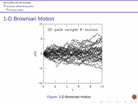
1-D Brownian Motion
Figure: 1-D Brownian motion
Intro to SDEs with with Examples
Stochastic Differential Equations
Brownian Motion
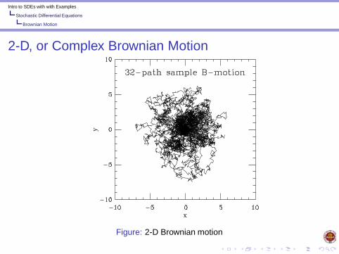
2-D, or Complex Brownian Motion
Figure: 2-D Brownian motion

Intro to SDEs with with Examples
Stochastic Differential Equations
Brownian Motion
Brownian Motion
w(t) = Brownian motion. Einstein’s relation gives diffusion coefficient
σ =
√2kTγ
m.
and probability density function for Brownian motion satisfies heatequation:
∂p(w , t)∂t
=12∂2p(w , t)
∂w2
Formal solution to LE is called an Ornstein-Uhlenbeck process
v(t) = v0e−γt + σe−γt∫ t
0eγsdw(s)

Intro to SDEs with with Examples
Stochastic Differential Equations
Brownian Motion
A Simple Stochastic Differential Equation
What does dw(t) mean?
w(t) = Δw1 +Δw2 + · · ·+Δwn
each increment is independent, and
E{ΔwiΔwj} = δijΔt
or infinitesimal version
Edw(t) = 0
E{dw(t) dw(s)} = δ(t − s) dt ds
Intro to SDEs with with Examples
Stochastic Differential Equations
Brownian Motion
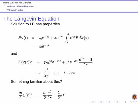
The Langevin EquationSolution to LE has properties
Ev(t) = v0e−γt + σe−γt∫ t
0eγsEdw(s)
= v0e−γt
and
E(v(t))2 = (v0)2e−2γt + σ2e−2γt e2γt − 1
2γ
→ σ2
2γas t → ∞
Something familiar about this?
m2
E(v)2 =m2σ2
2γ=
12
kT
Intro to SDEs with with Examples
Stochastic Differential Equations
Itô Calculus
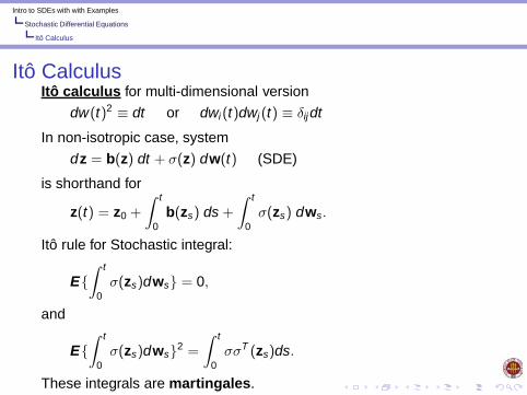
Itô CalculusItô calculus for multi-dimensional version
dw(t)2 ≡ dt or dwi(t)dwj (t) ≡ δij dt
In non-isotropic case, system
dz = b(z) dt + σ(z) dw(t) (SDE)
is shorthand for
z(t) = z0 +
∫ t
0b(zs) ds +
∫ t
0σ(zs) dws.
Itô rule for Stochastic integral:
E{∫ t
0σ(zs)dws} = 0,
and
E{∫ t
0σ(zs)dws}2 =
∫ t
0σσT (zs)ds.
These integrals are martingales.

Intro to SDEs with with Examples
Stochastic Differential Equations
Itô Calculus
A Standing Martingale
Figure: A standing martingale
Intro to SDEs with with Examples
Stochastic Differential Equations
Numerical Solution of SDEs
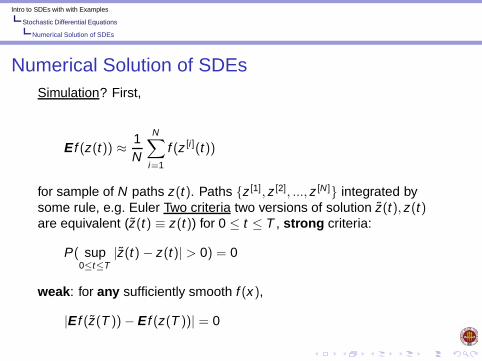
Numerical Solution of SDEsSimulation? First,
E f (z(t)) ≈ 1N
N∑i=1
f (z [i](t))
for sample of N paths z(t). Paths {z [1], z [2], ..., z [N]} integrated bysome rule, e.g. Euler Two criteria two versions of solution z̃(t), z(t)are equivalent (z̃(t) ≡ z(t)) for 0 ≤ t ≤ T , strong criteria:
P( sup0≤t≤T
|z̃(t) − z(t)| > 0) = 0
weak: for any sufficiently smooth f (x),
|E f (z̃(T ))− E f (z(T ))| = 0
Intro to SDEs with with Examples
Stochastic Differential Equations
Types of Solutions to SDEs
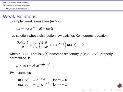
Weak SolutionsExample: weak simulation (m ≥ 0):
dx = −x |x |m−1dt + dw(t)
has solution whose distribution law satisfies Kolmogorov equation
∂p(x , t)∂t
=∂
∂x
(12
∂
∂x+ x |x |m−1
)p(x , t) → 0
when t → ∞. That is, x(t) becomes stationary. p(x , t → ∞), properlynormalized, is
p(x ,∞) = Nme− 2m+1 |x|m+1
.
Two examples
p(x ,∞) = e−2|x| for m = 0p(x ,∞) = 1√
πe−|x|2 for m = 1

Intro to SDEs with with Examples
Stochastic Differential Equations
Types of Solutions to SDEs
Strong SolutionsExample: a strong test,
dx = −λxdt + μxdw(t)
having formal solution
x(t) = x0 exp (−(λ+μ2
2)t + μw(t)). (1)
Notice x(t) → 0 as t → ∞. Many authors (Mitsui et al, Higham, ...)have studied stability regions, λ, μ, for asymptotic stability x(tn) → 0,when
tn = h1 + h2 + . . .+ hn → ∞may have varying stepsizes. Cases
t = T1 = n · h,
and h → h/2m = h′,
t = Tm = n2m · h′
Intro to SDEs with with Examples
Stochastic Differential Equations
Types of Solutions to SDEs
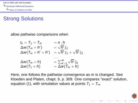
Strong Solutions
allow pathwise comparisons when
tn = T1 = Tm = n · hΔw(Tm + h′) =
√h′ ξ1
Δw(Tm + h′ + h′) =√
h′ ξ1 +√
h′ ξ2
. . .
Δw(Tm + h) =∑m
k=1
√h′ ξk
Δw(T1 + h) = Δw(Tm + h)
Here, one follows the pathwise convergence as m is changed. SeeKloeden and Platen, chapt. 9, p. 309. One compares "exact" solution,equation (1), with simulation values at points T1 = Tm.

Intro to SDEs with with Examples
Stochastic Differential Equations
Types of Solutions to SDEs
Strong Solutions
Numerical criteria similar: discrete times tk = kh, h = step size,T = Mh, andzk = numerical approx.,strong order β:
(E max0≤k≤M
|zk − z(tk )|2)1/2 ≤ K1hβ
weak order β: for f (z) ∈ C2β ,
|E f (zM)− E f (z(T ))| ≤ K2hβ

Intro to SDEs with with Examples
Stochastic Differential Equations
Examples
Examples
Example methods:Euler-Maruyama
zk+1 = zk + b(zk )h + σ(zk )ΔW
is strong order β = 1/2, weak order 1.Milstein
zk+1 =zk + b(zk )h + σ(zk )ΔW
+12σ(zk )σ
′(zk)(ΔW 2 − h)
is strong order β = 1, weak order 1

Intro to SDEs with with Examples
Stochastic Differential Equations
Higher-Order Methods
Higher-Order MethodsHigher order weak methods require modeling
Iij =∫ h
0widwj Ii0 =
∫ h
0wi(s)ds
Iijk =
∫ h
0wiwjdwk Iii0 =
∫ h
0w2
i ds
For example, for Runge-Kutta type methods
Iij ≈ 12ξiξj +
h2Ξij ,
Ii0 ≈ h2ξi ,
Iijk ≈ h2δijξk
Iii0 ≈ h2ξ2
i
Ξij is a model for∫
widwj − wjdwi .
Intro to SDEs with with Examples
Stochastic Differential Equations
Higher-Order Methods
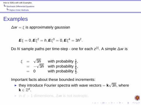
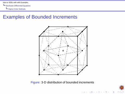
ExamplesΔw = ξ is approximately gaussian
Eξ = 0,Eξ2 = h,Eξ3 = 0,Eξ4 = 3h2.
Do N sample paths per time-step - one for each z [i]. A simple Δw is
ξ =√
3h with probability 16 ,
= −√3h with probability 1
6 ,= 0 with probability 2
3 .
Important facts about these bounded increments:� they introduce Fourier spectra with wave vectors = k
√3h, where
k ∈ Zd .
� in d > 1 dimensions, Δw is not isotropic.

Intro to SDEs with with Examples
Stochastic Differential Equations
Higher-Order Methods
ExamplesΔw = ξ is approximately gaussian
Eξ = 0,Eξ2 = h,Eξ3 = 0,Eξ4 = 3h2.
Do N sample paths per time-step - one for each z [i]. A simple Δw is
ξ =√
3h with probability 16 ,
= −√3h with probability 1
6 ,= 0 with probability 2
3 .
Important facts about these bounded increments:� they introduce Fourier spectra with wave vectors = k
√3h, where
k ∈ Zd .
� in d > 1 dimensions, Δw is not isotropic.
Intro to SDEs with with Examples
Stochastic Differential Equations
Higher-Order Methods
Examples of Bounded Increments
Figure: 3-D distribution of bounded increments
Intro to SDEs with with Examples
Stochastic Differential Equations
Some Applications
Some Applications
Some applications:
� Black-Scholes model for asset volatility� Langevin dynamics� shearing of light in inhomogeneous universes

Intro to SDEs with with Examples
Stochastic Differential Equations
Some Applications
Some Applications
Some applications:
� Black-Scholes model for asset volatility� Langevin dynamics� shearing of light in inhomogeneous universes
Intro to SDEs with with Examples
Stochastic Differential Equations
Some Applications
Some Applications
Some applications:
� Black-Scholes model for asset volatility� Langevin dynamics� shearing of light in inhomogeneous universes

Intro to SDEs with with Examples
Stochastic Differential Equations
Some Applications
Black-Scholes
Black-Scholes model. Let S = asset price, r = interest rate. Withoutvolatility,
dS = r S dt .
With efficient market hypothesis, fluctuations(S) ∝ S:
dS = rS dt + σS dw .
σ is called the volatility. Solution to SDE
S(t) = S0 e(r− 12σ
2)t+σw(t).

Intro to SDEs with with Examples
Stochastic Differential Equations
Some Applications
Langevin DynamicsLangevin dynamics: we want some physical quantity
E f =
∫p(x)f (x)dnx =
∫e−S(x)f (x)dnx∫
e−S(x)dnx.
To find a covering distribution q(x), αq(x) ≥ p(x), but α ≥ 1 is notlarge - difficult if n large.Alternative is Langevin dynamics:
dx(t) = −12∂S∂x
dt + dw(t),
and use
E f = limT→∞
1T
∫ T
0f (x(t))dt .
The following is sufficient for convergence: if |x| big,
x · ∂S∂x
> 1
Intro to SDEs with with Examples
Stochastic Differential Equations
Some Applications
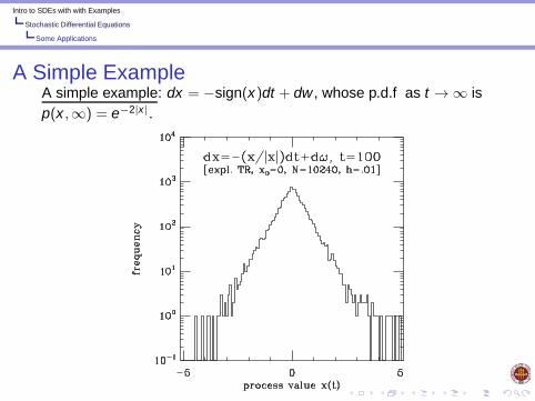
A Simple ExampleA simple example: dx = −sign(x)dt + dw , whose p.d.f as t → ∞ isp(x ,∞) = e−2|x|.
Intro to SDEs with with Examples
Stochastic Differential Equations
Some Applications
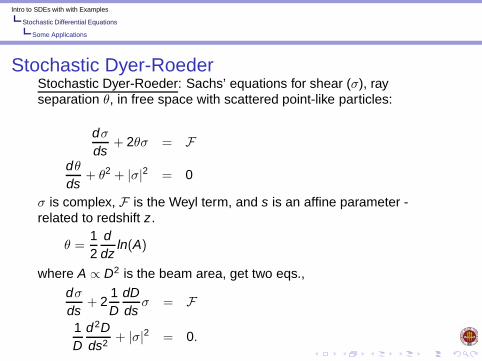
Stochastic Dyer-RoederStochastic Dyer-Roeder: Sachs’ equations for shear (σ), rayseparation θ, in free space with scattered point-like particles:
dσds
+ 2θσ = Fdθds
+ θ2 + |σ|2 = 0
σ is complex, F is the Weyl term, and s is an affine parameter -related to redshift z.
θ =12
ddz
ln(A)
where A ∝ D2 is the beam area, get two eqs.,
dσds
+ 21D
dDds
σ = F1D
d2Dds2 + |σ|2 = 0.

Intro to SDEs with with Examples
Stochastic Differential Equations
Some Applications
Stochastic Dyer-RoederIn Lagrangian coordinates (contract with redshift z), the Weyl term to1st order has derivatives of the gravitational potential Φ(x , y), withz = x + i y :
F =1c2 (1 + z)2 d2Φ
dz2 .
Light "sees" shearing forces orthogonal to congruence. Problem isessentially 2-D:
x
y
light ray
scattering plane
Figure: 2-D character of light scattering

Intro to SDEs with with Examples
Stochastic Differential Equations
Some Applications
Stochastic Dyer-RoederCorrelation length is about 7 cells, i.e. ∼ 7 Mpc at z = 0. Softened(2-3 cells) shears are normal in < 128 Mpc.
Figure: Shearing forces, from H. Couchman’s code

Intro to SDEs with with Examples
Stochastic Differential Equations
Some Applications
Stochastic Dyer-RoederMore useful form for 1st:
D2σ =
∫ s
0D2(s′)F(s′)ds′.
Expressing the affine parameter in terms of the redshift
s =
∫ z
0
dξ(1 + ξ)3
√1 +Ωξ)
Yields a generalized Dyer-Roeder eq.
(1 + z)(1 +Ωz)d2Ddz2
+(72Ωz +
Ω
2+ 3)
dDdz
+|σ(z)|2(1 + z)5 D = 0.

Intro to SDEs with with Examples
Stochastic Differential Equations
Some Applications
Stochastic Dyer-Roeder
Shear can be well approximated by
σ(z) = γ3Ω
8π(D(z))2 ×∫ z
0(D(ξ))2(1 + ξ)(1 +Ωξ)−
12 dw(ξ)
where w(z) is a complex (2-D) B-motion. Constant γ ≈ 0.62 wasdetermined by N-body simulations.

Intro to SDEs with with Examples
Stochastic Differential Equations
Some Applications
Stochastic Dyer-Roeder
Figure: Shear free Dyer-Roeder D(z)
Intro to SDEs with with Examples
Stochastic Differential Equations
Some Applications
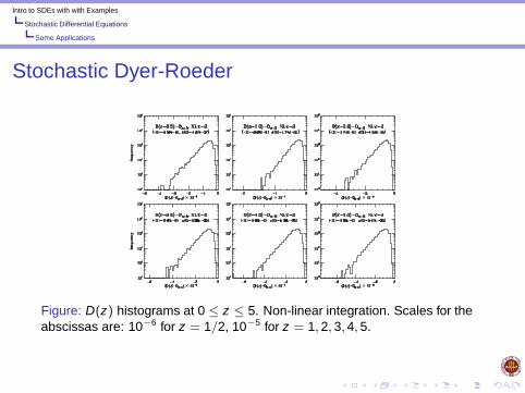
Stochastic Dyer-Roeder
Figure: D(z) histograms at 0 ≤ z ≤ 5. Non-linear integration. Scales for theabscissas are: 10−6 for z = 1/2, 10−5 for z = 1, 2, 3,4, 5.

Intro to SDEs with with Examples
Stability
Weak Solutions
Weak SimulationsRecall some basic rules of the Itô calculus
Edw(t) = 0
E{dw(t) dw(s)} = δ(t − s) dt ds
Multi-dimensional version
dwi(t)2 ≡ dt or dwi (t)dwj (t) ≡ δijdt
Usual z(t) ∈ C0 process:
dz = b(z) dt + σ(z) dw(t) (SDE)
is shorthand for
z(t) = z0 +
∫ t
0b(zs) ds +
∫ t
0σ(zs) dws.
Stochastic integral is non-anticipating. Important thing about Itô rule:
E{∫ t
0σ(zs)dws} = 0.

Intro to SDEs with with Examples
Stability
Weak Solutions
Weak SimulationsTaking the expression for z(t) for one step t → t + h,
z(t + h) = zt +
∫ t+h
tbs ds +
∫ t+h
tσs dws,
and substituting z(s) from the right-hand side into the left sideintegrals, e. g.∫ t+h
tb(zs) ds =
∫ t+h
tb(zt +
∫ s
tbudu +
∫ s
tσu dwu) ds.
Since t ≤ u ≤ s ≤ t + h and∫ s
tσudw(u) = O((s − t)1/2)
an expansion gives, including the∫σdw term, Picard-fashion, a
stochastic Taylor series (due to Wolfgang Wagner)

Intro to SDEs with with Examples
Stability
Weak Solutions
Weak SimulationsTruncating Taylor series to O(h) accuracy, we get Milstein’s method(scalar case):
z(t + h) = z(t) + hb(z(t)) + σ(z(t))Δω
+12σ′σ(Δω2 − h)
Again
Δω =√
h ξ
where ξ =zero-centered, univariate normal:
Eξ = 0, Eξ2 = 1.
Notice that because EΔω2 = h, Milstein’s term preserves theMartingale property
E12σ
′tσt (Δω2 − h) = 0.
Intro to SDEs with with Examples
Stability
Weak Solutions
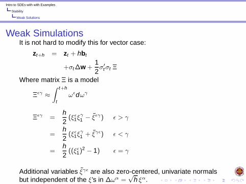
Weak SimulationsIt is not hard to modify this for vector case:
zt+h = zt + hbt
+σtΔw +12σ′
tσt Ξ
Where matrix Ξ is a model
Ξεγ ≈∫ t+h
tωεdωγ
Ξεγ =h2(ξε1ξ
γ1 − ξ̃εγ) ε > γ
=h2(ξε1ξ
γ1 + ξ̃γε) ε < γ
=h2((ξε1)
2 − 1) ε = γ
Additional variables ξ̃γε are also zero-centered, univariate normalsbut independent of the ξ’s in Δωα =
√h ξα.

Intro to SDEs with with Examples
Stability
Higher-Order Schemes
Higher-Order Schemes
Here is a second order accurate method. Writing b = A + B,
zαt+h = zα
t
+h2(Aα(zt+h) + Bα(zt + σtξ1 + (At + Bt )h)
+Aα(zt) + Bα(zt))
+12{σαβ(zt +
√12σtξ0 +
h2(At + Bt ))
+ σαβ(zt −√
12σtξ0 +
h2(At + Bt ))}ξβ1
+(∂βσαδt )σβε
t Ξεδ.
The first A(zt+h) is implicit.

Intro to SDEs with with Examples
Stability
Examples
An ExampleLet’s take a simple case, M > 0 (stable matrix),
dz = −Mzdt + dw
and write M = A + B, where I + hA is easy to invert. The semi-implicitalgorithm is
(I + hA) zt+h = (I − hB) zt +Δw
or
zt+h = (I + hA)−1((I − hB) zt +Δw)
In particular case A = B = 12M ,
zt+h = (I +h2
M)−1((I − h2
M)zt +Δw).
Stability of procedure will depend on L2 norm
||(I + h2
M)−1(I − h2
M)|| < 1.

Intro to SDEs with with Examples
Stability
Examples
An Example
Even in scalar case, when h is large enough (h > 2/M), |1− hM | > 1,but
|(1 − hM/2)/(1 + hM/2)| ≤ 1
for all h > 0.
Two dimensional case when scales of e.v.’s are very different:[dxdy
]= −1
2
[λ1 + λ2, λ1 − λ2
λ1 − λ2, λ1 + λ2
] [xy
]dt
+
[dw1(t)dw2(t)
].
which converges for ∀ λi > 0, but if λ1 λ2, the stepsizeh < 2/λ1 - too small to be useful. This is stiffness, justlike in the ODE case.

Intro to SDEs with with Examples
Stability
Examples
Another ExampleFor real, SPD matrix M :
dz = −Mzdt + dw.
The solution is formally
z(t) = e−Mtz(0) +∫ t
0eM(s−t)dw(s).
Large t corr. matrix approximates 12M−1:
Ezi(∞)zj(∞) =12[M−1]ij .
For big M , actual computational method is
Ezi(∞)zj(∞) ≈ 1T
∫ T
0zi(t)zj (t)dt
as T gets big, from the ergodic theorem.
Intro to SDEs with with Examples
Stability
Examples
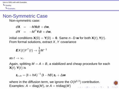
Non-Symmetric CaseNon-symmetric case:
dX = −MXdt + dw,
dY = −MT Ydt + dw,
initial conditions X(0) = Y(0) = 0. Same n−D w for both X(t),Y(t).From formal solutions, extract X ,Y covariance
EX (t)Y T (t) → 12
M−1
as t → ∞.
Again, splitting M = A + B, a stabilized and cheap procedure for eachX(t),Y(t) is
zt+h = (I + hA)−1(I − hB) zt +Δw
where in the diffusion term, we ignore the O(h3/2) contribution.Examples: A = diag(M), or A = tridiag(M)

Intro to SDEs with with Examples
Stability
Examples
A Test ProblemTest problem: M = UT TrU, where Tr = upper triangular,diag(Tr) = (1, . . . ,N), [Tr ]i,j ∈ N (0, 1), j > i . Random orthogonal Uby Pete Stewart’s procedure: S = diag(sign(u1))
U = SU0U1 . . .UN−2
where
Uk =
(Ik
HN−k
)
Hj = Householder transforms,
Hj = Ij − 2uuT
||u||2with j−length vectors u
u = x − ||x||e1,
each xi ∈ N (0, 1), i = 1, . . . , j . Also, cond(M) ∼ N.

Intro to SDEs with with Examples
Stability
Numerical Examples
Convergence of the Euler Method
1

Intro to SDEs with with Examples
Stability
Numerical Examples
Convergence of a Second-Order Method
1
Intro to SDEs with with Examples
Stability
Numerical Examples
More ExamplesMore general problems? Some has been done. Talay, Tubaro, andBally’s Euler estimates
|E f (z(T ))− E f (zn(T ))| ≤ hK (T )||f ||∞
T q
h = T/n = time step, q > 0 constant, and K (T ) is non-decreasing.Optimal choice of T is unclear. Example of Langevin dynamics,
dz(t) = −b(z)dt + dw(t), (2)
want z to converge to stationary. For large |z(t)|,E |z +Δz|2 ≤ E |z|2.
From eq. (2),
2z · b(z) ≥ 1
Discretization errors O(h) for Euler, O(h2) for 2nd order RK.
Intro to SDEs with with Examples
Stability
Numerical Examples
A Final Example
A final example model problem, where m ∈ Z+
dx = −x |x |m−1dt + dw(t)
Two procedures: Δω =√
h ξ,
xh = XTR(x0, ξ)
= x0 − h2(xeuler |xeuler |m−1 + x0|x0|m−1)
+Δω
xh = ITR(x0, ξ)
= x0 − h2(xh|xh|m−1 + x0|x0|m−1)
+Δω

Intro to SDEs with with Examples
Stability
Numerical Examples
A Final Example

Intro to SDEs with with Examples
Bibliography
Selected Bibliography
[1] P. E. Kloeden and E. Platen, Numerical Solution of StochasticDifferential Equations, Springer, 1999.[2] G. N. Milstein Numerical Integration of Stochastic DifferentialEquations, Kluwer, 1995.[3] W. Petersen, J. Comp. Physics, 113(1), July 1994.[4] W. Petersen, J. Stoch. Analysis and Applications, 22(4):989–1008, 2004.[5] W. Petersen, SIAM Journal on Numerical Analysis, 35(4): 1439,1998.[6] F. Buchmann and W. Petersen, Preconditioner..., SAM Report,2003.[7] G. W. Stewart, SIAM Journal on Numerical Analysis, 17(3), 1980.