the stochastic simulation algorithm

Computer Science Large Practical:The Stochastic Simulation Algorithm (SSA)

Stephen Gilmore

School of Informatics

Friday 5th October, 2012

Stephen Gilmore (School of Informatics) Stochastic simulation Friday 5th October, 2012 1 / 25

Stochastic: Random processes

Fundamental to the principle of stochastic modelling is the idea thatmolecular reactions are essentially random processes; it is impossibleto say with complete certainty the time at which the next reactionwithin a volume will occur.


Stochastic: Predictability of macroscopic states

In macroscopic systems, with a large number of interacting molecules,the randomness of this behaviour averages out so that the overallmacroscopic state of the system becomes highly predictable.

It is this property of large scale random systems that enables adeterministic approach to be adopted; however, the validity of thisassumption becomes strained in in vivo conditions as we examinesmall-scale cellular reaction environments with limited reactantpopulations.


Stochastic: Propensity function

As explicitly derived by Gillespie, the stochastic model uses basicNewtonian physics and thermodynamics to arrive at a form often termedthe propensity function that gives the probability aµ of reaction µoccurring in time interval (t, t + dt).

aµdt = hµcµdt

where the M reaction mechanisms are given an arbitrary index µ(1 ≤ µ ≤ M), hµ denotes the number of possible combinations of reactantmolecules involved in reaction µ, and cµ is a stochastic rate constant.


Stochastic: Grand probability function

The stochastic formulation proceeds by considering the grand probabilityfunction Pr(X; t) ≡ probability that there will be present in the volume Vat time t, Xi of species Si , where X ≡ (X1,X2, . . .XN) is a vector ofmolecular species populations.

Evidently, knowledge of this function provides a complete understanding ofthe probability distribution of all possible states at all times.


Stochastic: Infinitesimal time interval

By considering a discrete infinitesimal time interval (t, t + dt) in whicheither 0 or 1 reactions occur we see that there exist only M + 1 distinctconfigurations at time t that can lead to the state X at time t + dt.

Pr(X; t + dt)

= Pr(X; t) Pr(no state change over dt)

+∑M

µ=1 Pr(X− vµ; t) Pr(state change to X over dt)

where vµ is a stoichiometric vector defining the result of reaction µ onstate vector X, i.e. X→ X + vµ after an occurrence of reaction µ.


Stochastic: State change probabilities

Pr(no state change over dt)

1−M∑µ=1

aµ(X)dt

Pr(state change to X over dt)

M∑µ=1

Pr(X− vµ; t)aµ(X− vµ)dt


Stochastic: Partial derivatives

We are considering the behaviour of the system in the limit as dt tends tozero. This leads us to consider partial derivatives, which are defined thus:

∂ Pr(X; t)

∂t= lim

dt→0

Pr(X; t + dt)− Pr(X; t)

dt


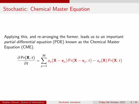
Stochastic: Chemical Master Equation

Applying this, and re-arranging the former, leads us to an importantpartial differential equation (PDE) known as the Chemical MasterEquation (CME).

∂ Pr(X; t)

∂t=

M∑µ=1

aµ(X− vµ) Pr(X− vµ; t)− aµ(X) Pr(X; t)


The problem with the Chemical Master Equation

The CME is really a set of nearly as many coupled ordinarydifferential equations as there are combinations of molecules that canexist in the system!

The CME can be solved analytically for only a very few very simplesystems, and numerical solutions are usually prohibitively difficult.

D. Gillespie and L. Petzold.

chapter Numerical Simulation for Biochemical Kinetics, in System Modellingin Cellular Biology, editors Z. Szallasi, J. Stelling and V. Periwal.

MIT Press, 2006.


Advertisement: Athena SWANLast day to take part

As part of the School of Informatics’ commitment to diversity, and toa workplace where all students are treated fairly, we have decided toundertake a gender equality culture survey.

The focus of this survey is gender diversity, as this is a cross-cuttingdiversity issue where we feel we can have the greatest positive impact;contributing to development and advancement of the School, for allour students.



The survey results will tell us what we are doing well in terms ofgender equality, and where we need to make any improvements.

The School is committed to using this data to improve our policiesand practices. This will also feed into our Athena SWAN application.

The link to the survey is https:

//www.survey.ed.ac.uk/informatics_student_culture2012/


https://www.survey.ed.ac.uk/informatics_student_culture2012/

https://www.survey.ed.ac.uk/informatics_student_culture2012/


Your response will be confidential and only anonymous results will beseen by management, and communicated to staff (students).

The survey should take only about 10 minutes to complete and willbe available until 5th October (today).


Stochastic simulation algorithms


Gillespie’s Stochastic Simulation Algorithm (SSA) is essentially an exactprocedure for numerically simulating the time evolution of a well-stirredchemically reacting system by taking proper account of the randomnessinherent in such a system.



Gillespie’s exact SSA (1977)

The algorithm takes time steps of variable length, based on the rateconstants and population size of each chemical species.

The probability of one reaction occurring relative to another isdictated by their relative propensity functions.

According to the correct probability distribution derived from thestatistical thermodynamics theory, a random variable is then used tochoose which reaction will occur, and another random variabledetermines how long the step will last.

The chemical populations are altered according to the stoichiometryof the reaction and the process is repeated.



Gillespie’s exact SSA (1977)As described by in “Stochastic Simulation Algorithms for Chemical Reactions” by Ahn,Cao and Watson, 2008

Suppose a biochemical system or pathway involves N molecularspecies S1, . . . ,SN.Xi (t) denotes the number of molecules of species Si at time t.

People would like to study the evolution of the state vectorX (t) = (X1(t), . . . ,XN(t)) given that the system was initially in thestate vector X (t0).

Example

The enzyme-substrate example had N = 4 molecular species, (E ,S ,C ,P),and the initial state vector X (t0) was (5, 5, 0, 0). If t = 200 we might findthat X (t) was (5, 0, 0, 5).




Suppose the system is composed of M reaction channelsR1, . . . ,RM.In a constant volume Ω, assume that the system is well-stirred and inthermal equilibrium at some constant temperature.

Example

The enzyme-substrate example had M = 3 reaction channels, f , b and p.




There are two important quantities in reaction channels Rj :

the state change vector vj = (v1j , . . . , vNj), andpropensity function aj .

vij is defined as the change in the Si molecules’ population caused byone Rj reaction,

aj(x)dt gives the probability that one Rj reaction will occur in thenext infinitesimal time interval [t, t + dt).

Example

The reaction f: E + S -> C has state change vector (−1,−1, 1, 0).




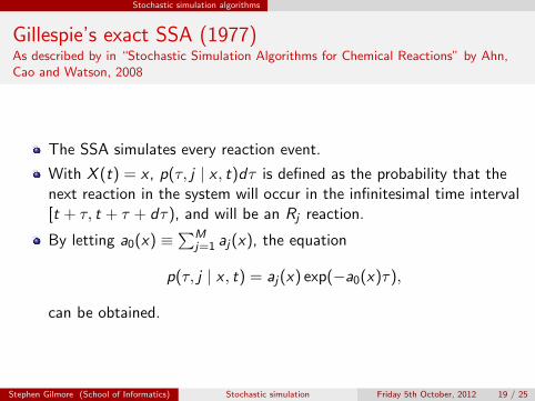
The SSA simulates every reaction event.

With X (t) = x , p(τ, j | x , t)dτ is defined as the probability that thenext reaction in the system will occur in the infinitesimal time interval[t + τ, t + τ + dτ), and will be an Rj reaction.

By letting a0(x) ≡∑M

j=1 aj(x), the equation

p(τ, j | x , t) = aj(x) exp(−a0(x)τ),

can be obtained.




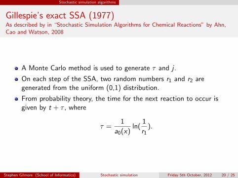
A Monte Carlo method is used to generate τ and j .

On each step of the SSA, two random numbers r1 and r2 aregenerated from the uniform (0,1) distribution.

From probability theory, the time for the next reaction to occur isgiven by t + τ , where

τ =1

a0(x)ln(

1

r1).




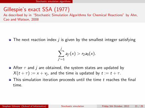
The next reaction index j is given by the smallest integer satisfying

j∑j ′=1

aj ′(x) > r2a0(x).

After τ and j are obtained, the system states are updated byX (t + τ) := x + vj , and the time is updated by t := t + τ .

This simulation iteration proceeds until the time t reaches the finaltime.



Sampling from a probability distribution

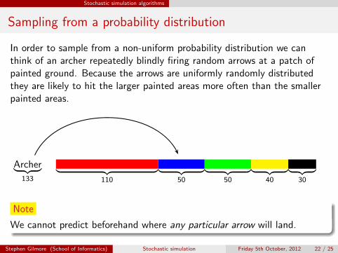
In order to sample from a non-uniform probability distribution we canthink of an archer repeatedly blindly firing random arrows at a patch ofpainted ground. Because the arrows are uniformly randomly distributedthey are likely to hit the larger painted areas more often than the smallerpainted areas.

︸︷︷︸110

︸︷︷︸50

︸︷︷︸50

︸︷︷︸40

︸︷︷︸30

Archer︸︷︷︸133

Note

We cannot predict beforehand where any particular arrow will land.



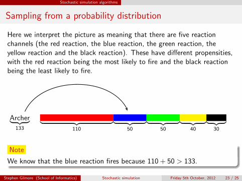
Sampling from a probability distribution

Here we interpret the picture as meaning that there are five reactionchannels (the red reaction, the blue reaction, the green reaction, theyellow reaction and the black reaction). These have different propensities,with the red reaction being the most likely to fire and the black reactionbeing the least likely to fire.

︸︷︷︸110

︸︷︷︸50

︸︷︷︸50

︸︷︷︸40

︸︷︷︸30

Archer︸︷︷︸133

Note

We know that the blue reaction fires because 110 + 50 > 133.



Gillespie’s SSA is a Monte Carlo Markov Chain simulation

The SSA is a Monte Carlo type method. With the SSA one mayapproximate any variable of interest by generating many trajectories andobserving the statistics of the values of the variable. Since manytrajectories are needed to obtain a reasonable approximation, the efficiencyof the SSA is of critical importance.



Excellent introductory papers

T.E. Turner, S. Schnell, and K. Burrage.

Stochastic approaches for modelling in vivo reactions.

Computational Biology and Chemistry, 28:165–178, 2004.

D. Gillespie and L. Petzold.

System Modelling in Cellular Biology, chapter Numerical Simulation forBiochemical Kinetics,.

MIT Press, 2006.


the stochastic simulation algorithm

Education