using r for personality research classical and modern test … · preliminaries reliability and...
TRANSCRIPT

Preliminaries Reliability and internal structure Types of reliability Calculating reliabilities 2 6= 1 Kappa
Using R for Personality ResearchClassical and Modern Test Theory
Part of a summer school sponsored byThe European Association for Personality Psychology
The International Society for the Study of Individual DifferencesThe Society for Multivariate Experimental Psychology
William Revelle
Department of PsychologyNorthwestern UniversityEvanston, Illinois USA
August, 2014
1 / 107

Preliminaries Reliability and internal structure Types of reliability Calculating reliabilities 2 6= 1 Kappa
Outline: Part I: Classical Test Theory
1 PreliminariesClassical test theoryCongeneric test theory
2 Reliability and internal structureEstimating reliability by split halvesDomain Sampling TheoryCoefficients based upon the internal structure of a testProblems with α
3 Types of reliabilityAlpha and its alternatives
4 Calculating reliabilitiesCongeneric measuresHierarchical structures
5 2 6= 1Multiple dimensions - falsely labeled as oneUsing score.items to find reliabilities of multiple scalesIntraclass correlationsICC of judges
6 KappaCohen’s kappaWeighted kappa
2 / 107
Preliminaries Reliability and internal structure Types of reliability Calculating reliabilities 2 6= 1 Kappa
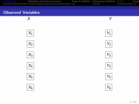
Observed Variables
X Y
X1
X2
X3
X4
X5
X6
Y1
Y2
Y3
Y4
Y5
Y6
3 / 107

Preliminaries Reliability and internal structure Types of reliability Calculating reliabilities 2 6= 1 Kappa
Latent Variables
ξ η
� ��
� ��
ξ1
ξ2
� ��
� ��
η1
η2
4 / 107

Preliminaries Reliability and internal structure Types of reliability Calculating reliabilities 2 6= 1 Kappa
Theory: A regression model of latent variables
ξ η
� ��
� ��
ξ1
ξ2
� ��
� ��
η1
η2
-
-
@@@@@@@@R
mζ1
��
mζ2@@I
5 / 107

Preliminaries Reliability and internal structure Types of reliability Calculating reliabilities 2 6= 1 Kappa
A measurement model for X – Correlated factors
δ X ξ
� ��� ��� ��� ��� ��� ��
δ1
δ2
δ3
δ4
δ5
δ6
-
-
-
-
-
-
X1
X2
X3
X4
X5
X6
� ��
� ��
ξ1
ξ2
QQQ
QQk
��
��
��+
QQQ
QQk
��
��
��+
6 / 107

Preliminaries Reliability and internal structure Types of reliability Calculating reliabilities 2 6= 1 Kappa
A measurement model for Y - uncorrelated factors
η Y ε
� ��
� ��
η1
η2
�����3
-QQQQQs
�����3
-QQQQQs
Y1
Y2
Y3
Y4
Y5
Y6
� ��� ��� ��� ��� ��� ��
ε1
ε2
ε3
ε4
ε5
ε6
�
�
�
�
�
�
7 / 107
Preliminaries Reliability and internal structure Types of reliability Calculating reliabilities 2 6= 1 Kappa
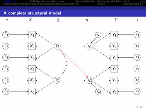
A complete structural model
δ X ξ η Y ε
� ��� ��� ��� ��� ��� ��
δ1
δ2
δ3
δ4
δ5
δ6
-
-
-
-
-
-
X1
X2
X3
X4
X5
X6
� ��
� ��
ξ1
ξ2
� ��
� ��
η1
η2
mζ1
��
mζ2@@I
QQQ
QQk
��
��
��+
QQQ
QQk
��
��
��+
�����3
-QQQQQs
�����3
-QQQQQs
-
-
@@@@@@@@R
Y1
Y2
Y3
Y4
Y5
Y6
� ��� ��� ��� ��� ��� ��
ε1
ε2
ε3
ε4
ε5
ε6
�
�
�
�
�
�
8 / 107
Preliminaries Reliability and internal structure Types of reliability Calculating reliabilities 2 6= 1 Kappa
Classical test theory
All data are befuddled with error
Now, suppose that we wish to ascertain thecorrespondence between a series of values, p, and anotherseries, q. By practical observation we evidently do notobtain the true objective values, p and q, but onlyapproximations which we will call p’ and q’. Obviously, p’is less closely connected with q’, than is p with q, for thefirst pair only correspond at all by the intermediation ofthe second pair; the real correspondence between p andq, shortly rpq has been ”attenuated” into rp′q′ (Spearman,1904, p 90).
9 / 107
Preliminaries Reliability and internal structure Types of reliability Calculating reliabilities 2 6= 1 Kappa
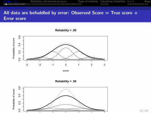
Classical test theory
All data are befuddled by error: Observed Score = True score +Error score
-3 -2 -1 0 1 2 3
0.0
0.2
0.4
0.6
Reliability = .80
score
Pro
babi
lity
of s
core
-3 -2 -1 0 1 2 3
0.0
0.2
0.4
0.6
Reliability = .50
score
Pro
babi
lity
of s
core
10 / 107
Preliminaries Reliability and internal structure Types of reliability Calculating reliabilities 2 6= 1 Kappa
Classical test theory
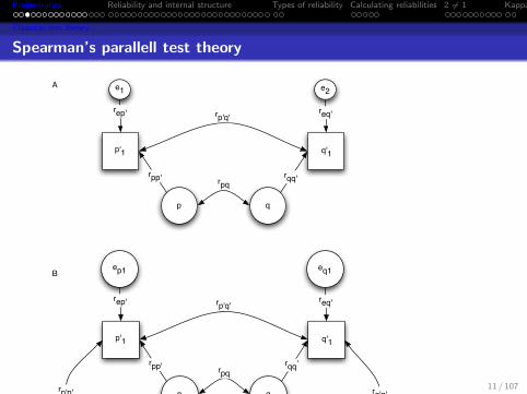
Spearman’s parallell test theory
p'1
p q
p'2
q'1
q'2
rpq
rp'q'
rp'p' rq'q'
rpp'
p'1
p q
q'1
rpq
rp'q'
e1 e2
rpp'
rep' req'
rqq'
rpp'
rqq'
rqq'
A
Bep1
ep2 eq2
eq1
rep' req'
rep' req'
11 / 107
Preliminaries Reliability and internal structure Types of reliability Calculating reliabilities 2 6= 1 Kappa
Classical test theory
Classical True score theory
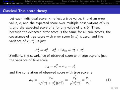
Let each individual score, x, reflect a true value, t, and an errorvalue, e, and the expected score over multiple observations of x ist, and the expected score of e for any value of p is 0. Then,because the expected error score is the same for all true scores, thecovariance of true score with error score (σte) is zero, and thevariance of x, σ2
x , is just
σ2x = σ2
t + σ2e + 2σte = σ2
t + σ2e .
Similarly, the covariance of observed score with true score is justthe variance of true score
σxt = σ2t + σte = σ2
t
and the correlation of observed score with true score is
ρxt =σxt√
(σ2t + σ2
e )(σ2t )
=σ2t√σ2xσ
2t
=σtσx. (1)
12 / 107
Preliminaries Reliability and internal structure Types of reliability Calculating reliabilities 2 6= 1 Kappa
Classical test theory
Classical Test Theory
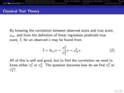
By knowing the correlation between observed score and true score,ρxt , and from the definition of linear regression predicted truescore, t̂, for an observed x may be found from
t̂ = bt.xx =σ2t
σ2x
x = ρ2xtx . (2)
All of this is well and good, but to find the correlation we need toknow either σ2
t or σ2e . The question becomes how do we find σ2
t orσ2e?.
13 / 107
Preliminaries Reliability and internal structure Types of reliability Calculating reliabilities 2 6= 1 Kappa
Classical test theory
Regression effects due to unreliability of measurement
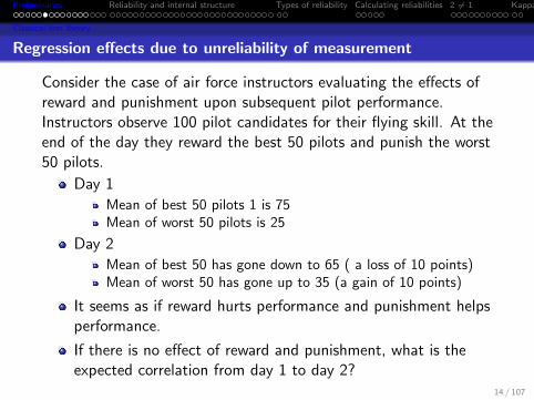
Consider the case of air force instructors evaluating the effects ofreward and punishment upon subsequent pilot performance.Instructors observe 100 pilot candidates for their flying skill. At theend of the day they reward the best 50 pilots and punish the worst50 pilots.
Day 1
Mean of best 50 pilots 1 is 75Mean of worst 50 pilots is 25
Day 2
Mean of best 50 has gone down to 65 ( a loss of 10 points)Mean of worst 50 has gone up to 35 (a gain of 10 points)
It seems as if reward hurts performance and punishment helpsperformance.
If there is no effect of reward and punishment, what is theexpected correlation from day 1 to day 2?
14 / 107

Preliminaries Reliability and internal structure Types of reliability Calculating reliabilities 2 6= 1 Kappa
Classical test theory
Correcting for attenuation
To ascertain the amount of this attenuation, and therebydiscover the true correlation, it appears necessary tomake two or more independent series of observations ofboth p and q. (Spearman, 1904, p 90)
Spearman’s solution to the problem of estimating the truerelationship between two variables, p and q, given observed scoresp’ and q’ was to introduce two or more additional variables thatcame to be called parallel tests. These were tests that had thesame true score for each individual and also had equal errorvariances. To Spearman (1904b p 90) this required finding “theaverage correlation between one and another of theseindependently obtained series of values” to estimate the reliabilityof each set of measures (rp′p′ , rq′q′), and then to find
rpq =rp′q′√
rp′p′rq′q′. (3)
15 / 107
Preliminaries Reliability and internal structure Types of reliability Calculating reliabilities 2 6= 1 Kappa
Classical test theory
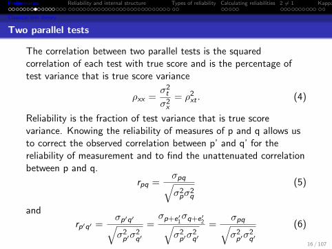
Two parallel tests
The correlation between two parallel tests is the squaredcorrelation of each test with true score and is the percentage oftest variance that is true score variance
ρxx =σ2t
σ2x
= ρ2xt . (4)
Reliability is the fraction of test variance that is true scorevariance. Knowing the reliability of measures of p and q allows usto correct the observed correlation between p’ and q’ for thereliability of measurement and to find the unattenuated correlationbetween p and q.
rpq =σpq√σ2pσ
2q
(5)
and
rp′q′ =σp′q′√σ2p′σ
2q′
=σp+e′1
σq+e′2√σ2p′σ
2q′
=σpq√σ2p′σ
2q′
(6)
16 / 107
Preliminaries Reliability and internal structure Types of reliability Calculating reliabilities 2 6= 1 Kappa
Classical test theory
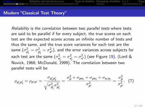
Modern “Classical Test Theory”
Reliability is the correlation between two parallel tests where testsare said to be parallel if for every subject, the true scores on eachtest are the expected scores across an infinite number of tests andthus the same, and the true score variances for each test are thesame (σ2
p′1= σ2
p′2= σ2
p′), and the error variances across subjects for
each test are the same (σ2e′1
= σ2e′2
= σ2e′) (see Figure 19), (Lord &
Novick, 1968; McDonald, 1999). The correlation between twoparallel tests will be
ρp′1p′2 = ρp′p′ =σp′1p′2√σ2p′1σ2p′2
=σ2p + σpe1 + σpe2 + σe1e2
σ2p′
=σ2p
σ2p′. (7)
17 / 107
Preliminaries Reliability and internal structure Types of reliability Calculating reliabilities 2 6= 1 Kappa
Classical test theory
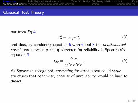
Classical Test Theory
but from Eq 4,σ2p = ρp′p′σ
2p′ (8)
and thus, by combining equation 5 with 6 and 8 the unattenuatedcorrelation between p and q corrected for reliability is Spearman’sequation 3
rpq =rp′q′√
rp′p′rq′q′. (9)
As Spearman recognized, correcting for attenuation could showstructures that otherwise, because of unreliability, would be hard todetect.
18 / 107
Preliminaries Reliability and internal structure Types of reliability Calculating reliabilities 2 6= 1 Kappa
Classical test theory
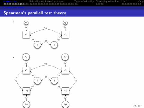
Spearman’s parallell test theory
p'1
p q
p'2
q'1
q'2
rpq
rp'q'
rp'p' rq'q'
rpp'
p'1
p q
q'1
rpq
rp'q'
e1 e2
rpp'
rep' req'
rqq'
rpp'
rqq'
rqq'
A
Bep1
ep2 eq2
eq1
rep' req'
rep' req'
19 / 107
Preliminaries Reliability and internal structure Types of reliability Calculating reliabilities 2 6= 1 Kappa
Classical test theory
When is a test a parallel test?
But how do we know that two tests are parallel? For just knowingthe correlation between two tests, without knowing the true scoresor their variance (and if we did, we would not bother withreliability), we are faced with three knowns (two variances and onecovariance) but ten unknowns (four variances and six covariances).That is, the observed correlation, rp′1p′2 represents the two known
variances s2p′1
and s2p′2
and their covariance sp′1p′2 . The model to
account for these three knowns reflects the variances of true anderror scores for p′1 and p′2 as well as the six covariances betweenthese four terms. In this case of two tests, by defining them to beparallel with uncorrelated errors, the number of unknowns drop tothree (for the true scores variances of p′1 and p′2 are set equal, asare the error variances, and all covariances with error are set tozero) and the (equal) reliability of each test may be found.
20 / 107

Preliminaries Reliability and internal structure Types of reliability Calculating reliabilities 2 6= 1 Kappa
Classical test theory
The problem of parallel tests
Unfortunately, according to this concept of parallel tests, thepossibility of one test being far better than the other is ignored.Parallel tests need to be parallel by construction or assumption andthe assumption of parallelism may not be tested. With the use ofmore tests, however, the number of assumptions can be relaxed(for three tests) and actually tested (for four or more tests).
21 / 107

Preliminaries Reliability and internal structure Types of reliability Calculating reliabilities 2 6= 1 Kappa
Congeneric test theory
Four congeneric tests – 1 latent factor
Four congeneric tests
V1 V2 V3 V4
F1
0.9 0.8 0.7 0.6
22 / 107
Preliminaries Reliability and internal structure Types of reliability Calculating reliabilities 2 6= 1 Kappa
Congeneric test theory
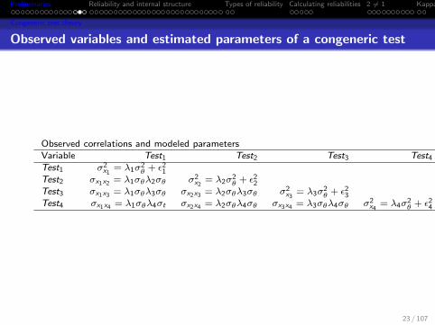
Observed variables and estimated parameters of a congeneric test
Observed correlations and modeled parametersVariable Test1 Test2 Test3 Test4
Test1 σ2x1
= λ1σ2θ + ε2
1Test2 σx1x2 = λ1σθλ2σθ σ2
x2= λ2σ
2θ + ε2
2Test3 σx1x3 = λ1σθλ3σθ σx2x3 = λ2σθλ3σθ σ2
x3= λ3σ
2θ + ε2
3Test4 σx1x4 = λ1σθλ4σt σx2x4 = λ2σθλ4σθ σx3x4 = λ3σθλ4σθ σ2
x4= λ4σ
2θ + ε2
4
23 / 107
Preliminaries Reliability and internal structure Types of reliability Calculating reliabilities 2 6= 1 Kappa
Congeneric test theory
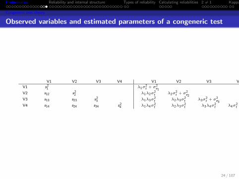
Observed variables and estimated parameters of a congeneric test
V1 V2 V3 V4 V1 V2 V3 V4
V1 s21 λ1σ
2t + σ2
e1V2 s12 s2
2 λ1λ2σ2t λ2σ
2t + σ2
e2V3 s13 s23 s2
3 λ1λ3σ2t λ2λ3σ
2t λ3σ
2t + σ2
e3V4 s14 s24 s34 s2
4 λ1λ4σ2t λ2λ3σ
2t λ3λ4σ
2t λ4σ
2t + σ2
e4
24 / 107
Preliminaries Reliability and internal structure Types of reliability Calculating reliabilities 2 6= 1 Kappa
But what if we don’t have three or more tests?
Unfortunately, with rare exceptions, we normally are faced withjust one test, not two, three or four. How then to estimate thereliability of that one test? Defined as the correlation between atest and a test just like it, reliability would seem to require asecond test. The traditional solution when faced with just one testis to consider the internal structure of that test. Letting reliabilitybe the ratio of true score variance to test score variance(Equation 1), or alternatively, 1 - the ratio of error variance to truescore variance, the problem becomes one of estimating the amountof error variance in the test. There are a number of solutions tothis problem that involve examining the internal structure of thetest. These range from considering the correlation between tworandom parts of the test to examining the structure of the itemsthemselves.
25 / 107
Preliminaries Reliability and internal structure Types of reliability Calculating reliabilities 2 6= 1 Kappa
Estimating reliability by split halves
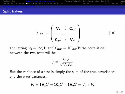
Split halves
ΣXX ′ =
Vx... Cxx′
. . . . . . . . . . . .
Cxx′... Vx′
(10)
and letting Vx = 1Vx1′ and CXX′ = 1CXX ′1′ the correlation
between the two tests will be
ρ =Cxx ′√VxVx ′
But the variance of a test is simply the sum of the true covariancesand the error variances:
Vx = 1Vx1′ = 1Ct1′ + 1Ve1′ = Vt + Ve
26 / 107
Preliminaries Reliability and internal structure Types of reliability Calculating reliabilities 2 6= 1 Kappa
Estimating reliability by split halves
Split halves
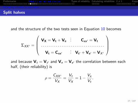
and the structure of the two tests seen in Equation 10 becomes
ΣXX ′ =
VX = Vt + Ve... Cxx′ = Vt
. . . . . . . . . . . . . . . . . . . . . . . . . . . . . . . . . .
Vt = Cxx′... Vt′ + Ve′ = VX ′
and because Vt = Vt′ and Ve = Ve′ the correlation between eachhalf, (their reliability) is
ρ =CXX ′
VX=
Vt
VX= 1− Ve
Vt.
27 / 107
Preliminaries Reliability and internal structure Types of reliability Calculating reliabilities 2 6= 1 Kappa
Estimating reliability by split halves
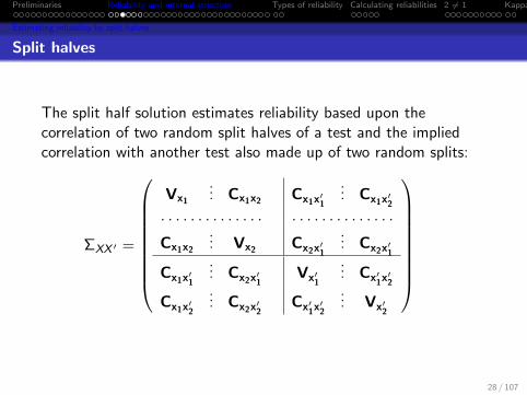
Split halves
The split half solution estimates reliability based upon thecorrelation of two random split halves of a test and the impliedcorrelation with another test also made up of two random splits:
ΣXX ′ =
Vx1
... Cx1x2 Cx1x′1
... Cx1x′2. . . . . . . . . . . . . . . . . . . . . . . . . . . .
Cx1x2
... Vx2 Cx2x′1
... Cx2x′1
Cx1x′1
... Cx2x′1Vx′1
... Cx′1x′2
Cx1x′2
... Cx2x′2Cx′1x′2
... Vx′2
28 / 107

Preliminaries Reliability and internal structure Types of reliability Calculating reliabilities 2 6= 1 Kappa
Estimating reliability by split halves
Split halves
Because the splits are done at random and the second test isparallel with the first test, the expected covariances between splitsare all equal to the true score variance of one split (Vt1), and thevariance of a split is the sum of true score and error variances:
ΣXX ′ =
Vt1 + Ve1
... Vt1 Vt1
... Vt1
. . . . . . . . . . . . . . . . . . . . . . . . . . . . . . . . . . . . . . . . . . . . . .
Vt1
... Vt1 + Ve1 Vt1
... Vt1
Vt1
... Vt1 Vt′1+ Ve′1
... Vt′1
Vt1
... Vt1 Vt′1
... Vt′1+ Ve′1
The correlation between a test made of up two halves withintercorrelation (r1 = Vt1/Vx1) with another such test is
rxx ′ =4Vt1√
(4Vt1 + 2Ve1)(4Vt1 + 2Ve1)=
4Vt1
2Vt1 + 2Vx1
=4r1
2r1 + 2
and thus
rxx ′ =2r1
1 + r1(11)
29 / 107
Preliminaries Reliability and internal structure Types of reliability Calculating reliabilities 2 6= 1 Kappa
Estimating reliability by split halves
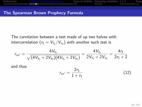
The Spearman Brown Prophecy Formula
The correlation between a test made of up two halves withintercorrelation (r1 = Vt1/Vx1) with another such test is
rxx ′ =4Vt1√
(4Vt1 + 2Ve1)(4Vt1 + 2Ve1)=
4Vt1
2Vt1 + 2Vx1
=4r1
2r1 + 2
and thus
rxx ′ =2r1
1 + r1(12)
30 / 107

Preliminaries Reliability and internal structure Types of reliability Calculating reliabilities 2 6= 1 Kappa
Estimating reliability by split halves
6,435 possible eight item splits of the 16 ability items
Split Half reliabilities of a test with 16 ability items
Split Half reliability
Frequency
0.74 0.76 0.78 0.80 0.82 0.84 0.86
050
100
150
Figure : There are 6,435 possible eight item splits of the 16 ability itemsof the ability data set. Of these, the maximum split half reliability is.87, the minimum is .73 and the average is .83. All possible splits werefound using the splitHalf function.
31 / 107
Preliminaries Reliability and internal structure Types of reliability Calculating reliabilities 2 6= 1 Kappa
Domain Sampling Theory
Domain sampling
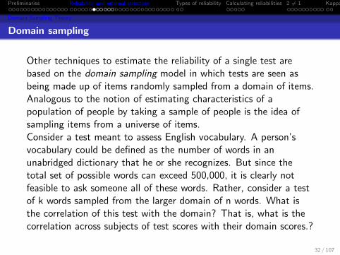
Other techniques to estimate the reliability of a single test arebased on the domain sampling model in which tests are seen asbeing made up of items randomly sampled from a domain of items.Analogous to the notion of estimating characteristics of apopulation of people by taking a sample of people is the idea ofsampling items from a universe of items.Consider a test meant to assess English vocabulary. A person’svocabulary could be defined as the number of words in anunabridged dictionary that he or she recognizes. But since thetotal set of possible words can exceed 500,000, it is clearly notfeasible to ask someone all of these words. Rather, consider a testof k words sampled from the larger domain of n words. What isthe correlation of this test with the domain? That is, what is thecorrelation across subjects of test scores with their domain scores.?
32 / 107

Preliminaries Reliability and internal structure Types of reliability Calculating reliabilities 2 6= 1 Kappa
Domain Sampling Theory
Correlation of an item with the domain
First consider the correlation of a single (randomly chosen) itemwith the domain. Let the domain score for an individual be Di andthe score on a particular item, j, be Xij . For ease of calculation,convert both of these to deviation scores. di = Di − D̄ andxij = Xij − X̄j . Then
rxjd =covxjd√σ2xjσ2d
.
Now, because the domain is just the sum of all the items, thedomain variance σ2
d is just the sum of all the item variances and allthe item covariances
σ2d =
n∑j=1
n∑k=1
covxjk =n∑
j=1
σ2xj
+n∑
j=1
∑k 6=j
covxjk .
33 / 107
Preliminaries Reliability and internal structure Types of reliability Calculating reliabilities 2 6= 1 Kappa
Domain Sampling Theory
Correlation of an item with the domain
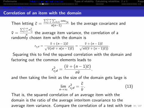
Then letting c̄ =∑j=n
j=1
∑k 6=j covxjk
n(n−1) be the average covariance and
v̄ =
∑j=nj=1 σ
2xj
n the average item variance, the correlation of arandomly chosen item with the domain is
rxjd =v̄ + (n − 1)c̄√
v̄(nv̄ + n(n − 1)c̄)=
v̄ + (n − 1)c̄√nv̄(v̄ + (n − 1)c̄))
.
Squaring this to find the squared correlation with the domain andfactoring out the common elements leads to
r 2xjd
=(v̄ + (n − 1)c̄)
nv̄.
and then taking the limit as the size of the domain gets large is
limn→∞
r 2xjd
=c̄
v̄. (13)
That is, the squared correlation of an average item with thedomain is the ratio of the average interitem covariance to theaverage item variance. Compare the correlation of a test with truescore (Eq 4) with the correlation of an item to the domain score(Eq 14). Although identical in form, the former makes assumptionsabout true score and error, the latter merely describes the domainas a large set of similar items.
34 / 107
Preliminaries Reliability and internal structure Types of reliability Calculating reliabilities 2 6= 1 Kappa
Domain Sampling Theory
Domain sampling – correlation of an item with the domain
limn→∞
r 2xjd
=c̄
v̄. (14)
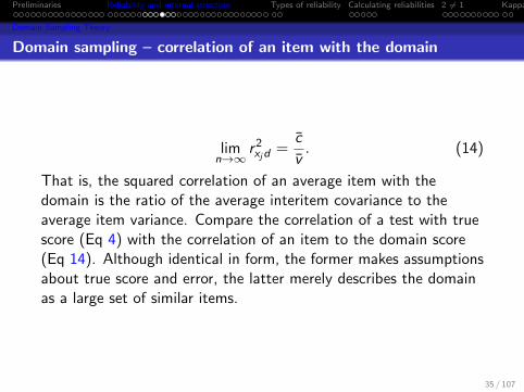
That is, the squared correlation of an average item with thedomain is the ratio of the average interitem covariance to theaverage item variance. Compare the correlation of a test with truescore (Eq 4) with the correlation of an item to the domain score(Eq 14). Although identical in form, the former makes assumptionsabout true score and error, the latter merely describes the domainas a large set of similar items.
35 / 107
Preliminaries Reliability and internal structure Types of reliability Calculating reliabilities 2 6= 1 Kappa
Domain Sampling Theory
Correlation of a test with the domain
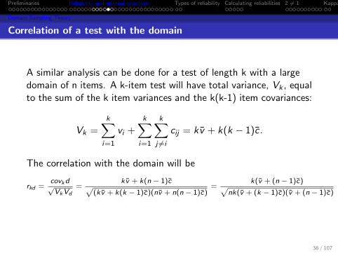
A similar analysis can be done for a test of length k with a largedomain of n items. A k-item test will have total variance, Vk , equalto the sum of the k item variances and the k(k-1) item covariances:
Vk =k∑
i=1
vi +k∑
i=1
k∑j 6=i
cij = kv̄ + k(k − 1)c̄.
The correlation with the domain will be
rkd =covkd√VkVd
=kv̄ + k(n − 1)c̄√
(kv̄ + k(k − 1)c̄)(nv̄ + n(n − 1)c̄)=
k(v̄ + (n − 1)c̄)√nk(v̄ + (k − 1)c̄)(v̄ + (n − 1)c̄)
36 / 107
Preliminaries Reliability and internal structure Types of reliability Calculating reliabilities 2 6= 1 Kappa
Domain Sampling Theory
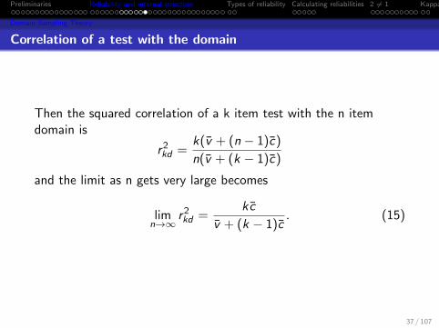
Correlation of a test with the domain
Then the squared correlation of a k item test with the n itemdomain is
r 2kd =
k(v̄ + (n − 1)c̄)
n(v̄ + (k − 1)c̄)
and the limit as n gets very large becomes
limn→∞
r 2kd =
kc̄
v̄ + (k − 1)c̄. (15)
37 / 107

Preliminaries Reliability and internal structure Types of reliability Calculating reliabilities 2 6= 1 Kappa
Coefficients based upon the internal structure of a test
Coefficient α
Find the correlation of a test with a test just like it based upon theinternal structure of the first test. Basically, we are just estimatingthe error variance of the individual items.
α = rxx =σ2t
σ2x
=k2 σ
2x−∑σ2i
k(k−1)
σ2x
=k
k − 1
σ2x −
∑σ2i
σ2x
(16)
38 / 107

Preliminaries Reliability and internal structure Types of reliability Calculating reliabilities 2 6= 1 Kappa
Coefficients based upon the internal structure of a test
Alpha varies by the number of items and the inter item correlation
0 20 40 60 80 100
0.4
0.5
0.6
0.7
0.8
0.9
Alpha varies by r and number of items
Number of items
alpha
r=.2
r=.1
r=.05
39 / 107
Preliminaries Reliability and internal structure Types of reliability Calculating reliabilities 2 6= 1 Kappa
Coefficients based upon the internal structure of a test
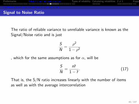
Signal to Noise Ratio
The ratio of reliable variance to unreliable variance is known as theSignal/Noise ratio and is just
S
N=
ρ2
1− ρ2
, which for the same assumptions as for α, will be
S
N=
nr̄
1− r̄. (17)
That is, the S/N ratio increases linearly with the number of itemsas well as with the average intercorrelation
40 / 107

Preliminaries Reliability and internal structure Types of reliability Calculating reliabilities 2 6= 1 Kappa
Coefficients based upon the internal structure of a test
Alpha vs signal/noise: and r and n
0 20 40 60 80 100
0.0
0.2
0.4
0.6
0.8
1.0
Alpha
Number of items
alpha
r = .05
r = .01
r = .4
r = .1
r = .2r = .3
0 20 40 60 80 100
010
2030
4050
60
Signal/Noise
Number of items
S/N
r = .05r = .01
r = .4
r = .1
r = .2
r = .3
41 / 107

Preliminaries Reliability and internal structure Types of reliability Calculating reliabilities 2 6= 1 Kappa
Coefficients based upon the internal structure of a test
Find alpha using the alpha function
> alpha(bfi[16:20])
Reliability analysisCall: alpha(x = bfi[16:20])
raw_alpha std.alpha G6(smc) average_r mean sd0.81 0.81 0.8 0.46 15 5.8
Reliability if an item is dropped:raw_alpha std.alpha G6(smc) average_r
N1 0.75 0.75 0.70 0.42N2 0.76 0.76 0.71 0.44N3 0.75 0.76 0.74 0.44N4 0.79 0.79 0.76 0.48N5 0.81 0.81 0.79 0.51
Item statisticsn r r.cor mean sd
N1 990 0.81 0.78 2.8 1.5N2 990 0.79 0.75 3.5 1.5N3 997 0.79 0.72 3.2 1.5N4 996 0.71 0.60 3.1 1.5N5 992 0.67 0.52 2.9 1.6
42 / 107
Preliminaries Reliability and internal structure Types of reliability Calculating reliabilities 2 6= 1 Kappa
Coefficients based upon the internal structure of a test
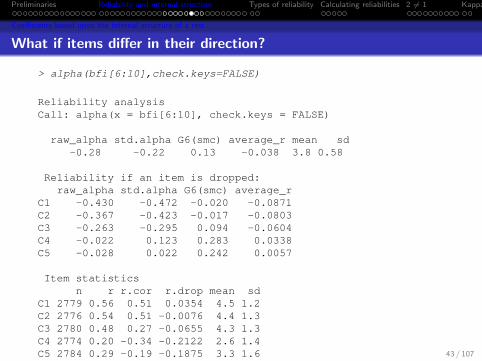
What if items differ in their direction?
> alpha(bfi[6:10],check.keys=FALSE)
Reliability analysisCall: alpha(x = bfi[6:10], check.keys = FALSE)
raw_alpha std.alpha G6(smc) average_r mean sd-0.28 -0.22 0.13 -0.038 3.8 0.58
Reliability if an item is dropped:raw_alpha std.alpha G6(smc) average_r
C1 -0.430 -0.472 -0.020 -0.0871C2 -0.367 -0.423 -0.017 -0.0803C3 -0.263 -0.295 0.094 -0.0604C4 -0.022 0.123 0.283 0.0338C5 -0.028 0.022 0.242 0.0057
Item statisticsn r r.cor r.drop mean sd
C1 2779 0.56 0.51 0.0354 4.5 1.2C2 2776 0.54 0.51 -0.0076 4.4 1.3C3 2780 0.48 0.27 -0.0655 4.3 1.3C4 2774 0.20 -0.34 -0.2122 2.6 1.4C5 2784 0.29 -0.19 -0.1875 3.3 1.6 43 / 107

Preliminaries Reliability and internal structure Types of reliability Calculating reliabilities 2 6= 1 Kappa
Coefficients based upon the internal structure of a test
But what if some items are reversed keyed?
alpha(bfi[6:10])
Reliability analysisCall: alpha(x = bfi[6:10])
raw_alpha std.alpha G6(smc) average_r mean sd0.73 0.73 0.69 0.35 3.8 0.58
Reliability if an item is dropped:raw_alpha std.alpha G6(smc) average_r
C1 0.69 0.70 0.64 0.36C2 0.67 0.67 0.62 0.34C3 0.69 0.69 0.64 0.36C4- 0.65 0.66 0.60 0.33C5- 0.69 0.69 0.63 0.36Item statistics
n r r.cor r.drop mean sdC1 2779 0.67 0.54 0.45 4.5 1.2C2 2776 0.71 0.60 0.50 4.4 1.3C3 2780 0.67 0.54 0.46 4.3 1.3C4- 2774 0.73 0.64 0.55 2.6 1.4C5- 2784 0.68 0.57 0.48 3.3 1.6Warning message: In alpha(bfi[6:10]) :
Some items were negatively correlated with total scale and were automatically reversed44 / 107
Preliminaries Reliability and internal structure Types of reliability Calculating reliabilities 2 6= 1 Kappa
Coefficients based upon the internal structure of a test
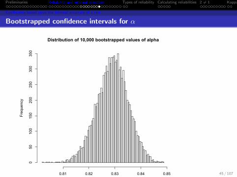
Bootstrapped confidence intervals for α
Distribution of 10,000 bootstrapped values of alpha
Alpha for 16 ability items
Frequency
0.81 0.82 0.83 0.84 0.85
050
100
150
200
250
300
350
45 / 107
Preliminaries Reliability and internal structure Types of reliability Calculating reliabilities 2 6= 1 Kappa
Problems with α
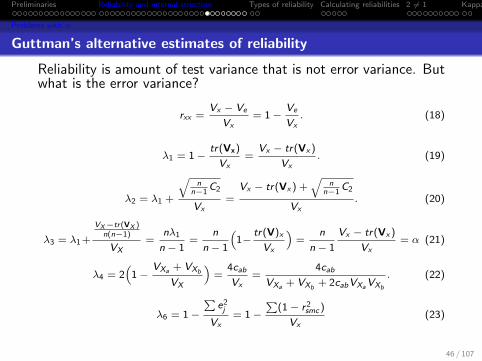
Guttman’s alternative estimates of reliability
Reliability is amount of test variance that is not error variance. Butwhat is the error variance?
rxx =Vx − Ve
Vx= 1−
Ve
Vx. (18)
λ1 = 1−tr(Vx)
Vx=
Vx − tr(Vx )
Vx. (19)
λ2 = λ1 +
√n
n−1C2
Vx=
Vx − tr(Vx ) +√
nn−1
C2
Vx. (20)
λ3 = λ1 +
VX−tr(VX )n(n−1)
VX=
nλ1
n − 1=
n
n − 1
(1−
tr(V)x
Vx
)=
n
n − 1
Vx − tr(Vx )
Vx= α (21)
λ4 = 2(
1−VXa + VXb
VX
)=
4cab
Vx=
4cab
VXa + VXb+ 2cabVXaVXb
. (22)
λ6 = 1−∑
e2j
Vx= 1−
∑(1− r2
smc)
Vx(23)
46 / 107
Preliminaries Reliability and internal structure Types of reliability Calculating reliabilities 2 6= 1 Kappa
Problems with α
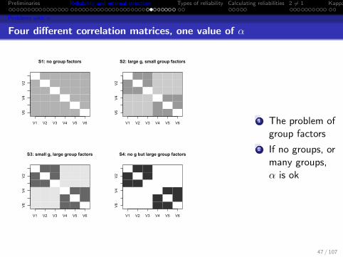
Four different correlation matrices, one value of α
S1: no group factors
V1 V2 V3 V4 V5 V6
V6
V4
V2
S2: large g, small group factors
V1 V2 V3 V4 V5 V6
V6
V4
V2
S3: small g, large group factors
V1 V2 V3 V4 V5 V6
V6
V4
V2
S4: no g but large group factors
V1 V2 V3 V4 V5 V6
V6
V4
V2
1 The problem ofgroup factors
2 If no groups, ormany groups,α is ok
47 / 107
Preliminaries Reliability and internal structure Types of reliability Calculating reliabilities 2 6= 1 Kappa
Problems with α
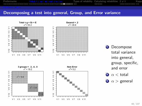
Decomposing a test into general, Group, and Error variance
Total = g + Gr + E
V 1 V 3 V 5 V 7 V 9 V 11
V 1
2V
9V
7V
5V
3V
1
σ2= 53.2General = .2
V 1 V 3 V 5 V 7 V 9 V 11V
12
V 9
V 7
V 5
V 3
V 1
σ2= 28.8
3 groups = .3, .4, .5
V 1 V 3 V 5 V 7 V 9 V 11
V 1
2V
9V
7V
5V
3V
1
σ2 = 19.2
σ2 = 10.8
σ2 = 6.4
σ2 = 2
Item Error
V 1 V 3 V 5 V 7 V 9 V 11
V 1
2V
9V
7V
5V
3V
1
σ2= 5.2
1 Decomposetotal varianceinto general,group, specific,and error
2 α < total
3 α > general
48 / 107
Preliminaries Reliability and internal structure Types of reliability Calculating reliabilities 2 6= 1 Kappa
Problems with α
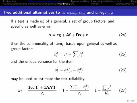
Two additional alternatives to α: ωhierarchical and omegatotal
If a test is made up of a general, a set of group factors, andspecific as well as error:
x = cg + Af + Ds + e (24)
then the communality of itemj , based upon general as well asgroup factors,
h2j = c2
j +∑
f 2ij (25)
and the unique variance for the item
u2j = σ2
j (1− h2j ) (26)
may be used to estimate the test reliability.
ωt =1cc′1′ + 1AA′1′
Vx= 1−
∑(1− h2
j )
Vx= 1−
∑u2
Vx(27)
49 / 107

Preliminaries Reliability and internal structure Types of reliability Calculating reliabilities 2 6= 1 Kappa
Problems with α
McDonald (1999) introduced two different forms for ω
ωt =1cc′1′ + 1AA′1′
Vx= 1−
∑(1− h2
j )
Vx= 1−
∑u2
Vx(28)
and
ωh =1cc′1
Vx=
(∑
Λi )2∑∑
Rij. (29)
These may both be find by factoring the correlation matrix andfinding the g and group factor loadings using the omega function.
50 / 107
Preliminaries Reliability and internal structure Types of reliability Calculating reliabilities 2 6= 1 Kappa
Problems with α
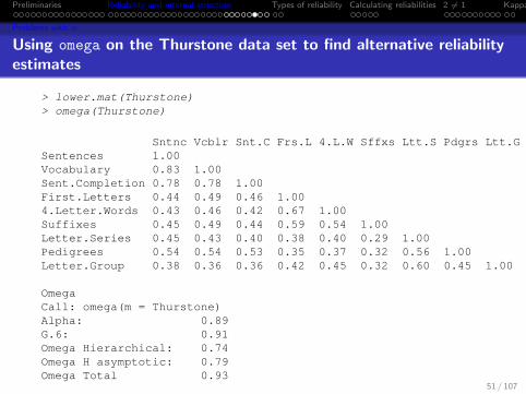
Using omega on the Thurstone data set to find alternative reliabilityestimates
> lower.mat(Thurstone)> omega(Thurstone)
Sntnc Vcblr Snt.C Frs.L 4.L.W Sffxs Ltt.S Pdgrs Ltt.GSentences 1.00Vocabulary 0.83 1.00Sent.Completion 0.78 0.78 1.00First.Letters 0.44 0.49 0.46 1.004.Letter.Words 0.43 0.46 0.42 0.67 1.00Suffixes 0.45 0.49 0.44 0.59 0.54 1.00Letter.Series 0.45 0.43 0.40 0.38 0.40 0.29 1.00Pedigrees 0.54 0.54 0.53 0.35 0.37 0.32 0.56 1.00Letter.Group 0.38 0.36 0.36 0.42 0.45 0.32 0.60 0.45 1.00
OmegaCall: omega(m = Thurstone)Alpha: 0.89G.6: 0.91Omega Hierarchical: 0.74Omega H asymptotic: 0.79Omega Total 0.93
51 / 107
Preliminaries Reliability and internal structure Types of reliability Calculating reliabilities 2 6= 1 Kappa
Problems with α
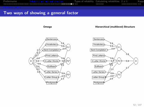
Two ways of showing a general factor
Omega
Sentences
Vocabulary
Sent.Completion
First.Letters
4.Letter.Words
Suffixes
Letter.Series
Letter.Group
Pedigrees
F1*
0.60.60.5
0.2
F2*0.60.5
0.4
F3*0.60.50.3
g
0.70.70.70.60.60.60.60.50.6
Hierarchical (multilevel) Structure
Sentences
Vocabulary
Sent.Completion
First.Letters
4.Letter.Words
Suffixes
Letter.Series
Letter.Group
Pedigrees
F1
0.90.90.8
0.4
F20.90.7
0.6
0.2
F30.80.60.5
g
0.8
0.8
0.7
52 / 107

Preliminaries Reliability and internal structure Types of reliability Calculating reliabilities 2 6= 1 Kappa
Problems with α
omega function does a Schmid Leiman transformation
> omega(Thurstone,sl=FALSE)
OmegaCall: omega(m = Thurstone, sl = FALSE)Alpha: 0.89G.6: 0.91Omega Hierarchical: 0.74Omega H asymptotic: 0.79Omega Total 0.93Schmid Leiman Factor loadings greater than 0.2
g F1* F2* F3* h2 u2 p2Sentences 0.71 0.57 0.82 0.18 0.61Vocabulary 0.73 0.55 0.84 0.16 0.63Sent.Completion 0.68 0.52 0.73 0.27 0.63First.Letters 0.65 0.56 0.73 0.27 0.574.Letter.Words 0.62 0.49 0.63 0.37 0.61Suffixes 0.56 0.41 0.50 0.50 0.63Letter.Series 0.59 0.61 0.72 0.28 0.48Pedigrees 0.58 0.23 0.34 0.50 0.50 0.66Letter.Group 0.54 0.46 0.53 0.47 0.56With eigenvalues of:
g F1* F2* F3*3.58 0.96 0.74 0.71
53 / 107

Preliminaries Reliability and internal structure Types of reliability Calculating reliabilities 2 6= 1 Kappa
Types of reliability
Internal consistency
αωhierarchical
ωtotal
β
Intraclass
Agreement
Test-retest, alternateform
Generalizability
Internal consistency
alpha,score.items
omega
iclust
icc
wkappa,cohen.kappa
cor
aov
54 / 107

Preliminaries Reliability and internal structure Types of reliability Calculating reliabilities 2 6= 1 Kappa
Alpha and its alternatives
Alpha and its alternatives
Reliability = σ2tσ2x
= 1− σ2eσ2x
If there is another test, then σt = σt1t2 (covariance of test X1
with test X2 = Cxx)But, if there is only one test, we can estimate σ2
t based uponthe observed covariances within test 1How do we find σ2
e ?The worst case, (Guttman case 1) all of an item’s variance iserror and thus the error variance of a test X withvariance-covariance Cx
Cx = σ2e = diag(Cx)
λ1 = Cx−diag(Cx )Cx
A better case (Guttman case 3, α) is that that the averagecovariance between the items on the test is the same as theaverage true score variance for each item.
Cx = σ2e = diag(Cx)
λ3 = α = λ1 ∗ nn−1 = (Cx−diag(Cx ))∗n/(n−1)
Cx
55 / 107
Preliminaries Reliability and internal structure Types of reliability Calculating reliabilities 2 6= 1 Kappa
Alpha and its alternatives
Guttman 6: estimating using the Squared Multiple Correlation
Reliability = σ2tσ2x
= 1− σ2eσ2x
Estimate true item variance as squared multiple correlationwith other items
λ6 = (Cx−diag(Cx )+Σ(smci )Cx
This takes observed covariance, subtracts the diagonal, andreplaces with the squared multiple correlationSimilar to α which replaces with average inter-item covariance
Squared Multiple Correlation is found by smc and is justsmci = 1− 1/R−1
ii
56 / 107

Preliminaries Reliability and internal structure Types of reliability Calculating reliabilities 2 6= 1 Kappa
Congeneric measures
Alpha and its alternatives: Case 1: congeneric measures
First, create some simulated data with a known structure> set.seed(42)> v4 <- sim.congeneric(N=200,short=FALSE)> str(v4) #show the structure of the resulting objectList of 6$ model : num [1:4, 1:4] 1 0.56 0.48 0.4 0.56 1 0.42 0.35 0.48 0.42 .....- attr(*, "dimnames")=List of 2.. ..$ : chr [1:4] "V1" "V2" "V3" "V4".. ..$ : chr [1:4] "V1" "V2" "V3" "V4"$ pattern : num [1:4, 1:5] 0.8 0.7 0.6 0.5 0.6 .....- attr(*, "dimnames")=List of 2.. ..$ : chr [1:4] "V1" "V2" "V3" "V4".. ..$ : chr [1:5] "theta" "e1" "e2" "e3" ...$ r : num [1:4, 1:4] 1 0.546 0.466 0.341 0.546 .....- attr(*, "dimnames")=List of 2.. ..$ : chr [1:4] "V1" "V2" "V3" "V4".. ..$ : chr [1:4] "V1" "V2" "V3" "V4"$ latent : num [1:200, 1:5] 1.371 -0.565 0.363 0.633 0.404 .....- attr(*, "dimnames")=List of 2.. ..$ : NULL.. ..$ : chr [1:5] "theta" "e1" "e2" "e3" ...$ observed: num [1:200, 1:4] -0.104 -0.251 0.993 1.742 -0.503 .....- attr(*, "dimnames")=List of 2.. ..$ : NULL.. ..$ : chr [1:4] "V1" "V2" "V3" "V4"$ N : num 200- attr(*, "class")= chr [1:2] "psych" "sim"
57 / 107

Preliminaries Reliability and internal structure Types of reliability Calculating reliabilities 2 6= 1 Kappa
Congeneric measures
A congeneric model
> f1 <- fa(v4$model)> fa.diagram(f1)
Four congeneric tests
V1 V2 V3 V4
F1
0.9 0.8 0.7 0.6
> v4$modelV1 V2 V3 V4
V1 1.00 0.56 0.48 0.40V2 0.56 1.00 0.42 0.35V3 0.48 0.42 1.00 0.30V4 0.40 0.35 0.30 1.00
> round(cor(v4$observed),2)V1 V2 V3 V4
V1 1.00 0.55 0.47 0.34V2 0.55 1.00 0.38 0.30V3 0.47 0.38 1.00 0.31V4 0.34 0.30 0.31 1.00
58 / 107

Preliminaries Reliability and internal structure Types of reliability Calculating reliabilities 2 6= 1 Kappa
Congeneric measures
Find α and related stats for the simulated data
> alpha(v4$observed)
Reliability analysisCall: alpha(x = v4$observed)
raw_alpha std.alpha G6(smc) average_r mean sd0.71 0.72 0.67 0.39 -0.036 0.72
Reliability if an item is dropped:raw_alpha std.alpha G6(smc) average_r
V1 0.59 0.60 0.50 0.33V2 0.63 0.64 0.55 0.37V3 0.65 0.66 0.59 0.40V4 0.72 0.72 0.64 0.46
Item statisticsn r r.cor r.drop mean sd
V1 200 0.80 0.72 0.60 -0.015 0.93V2 200 0.76 0.64 0.53 -0.060 0.98V3 200 0.73 0.59 0.50 -0.119 0.92V4 200 0.66 0.46 0.40 0.049 1.09
59 / 107
Preliminaries Reliability and internal structure Types of reliability Calculating reliabilities 2 6= 1 Kappa
Hierarchical structures
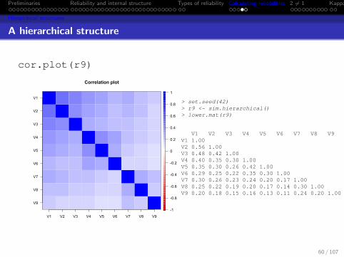
A hierarchical structure
cor.plot(r9)
Correlation plot
V1 V2 V3 V4 V5 V6 V7 V8 V9
V9
V8
V7
V6
V5
V4
V3
V2
V1
-1
-0.8
-0.6
-0.4
-0.2
0
0.2
0.4
0.6
0.8
1
> set.seed(42)> r9 <- sim.hierarchical()> lower.mat(r9)
V1 V2 V3 V4 V5 V6 V7 V8 V9V1 1.00V2 0.56 1.00V3 0.48 0.42 1.00V4 0.40 0.35 0.30 1.00V5 0.35 0.30 0.26 0.42 1.00V6 0.29 0.25 0.22 0.35 0.30 1.00V7 0.30 0.26 0.23 0.24 0.20 0.17 1.00V8 0.25 0.22 0.19 0.20 0.17 0.14 0.30 1.00V9 0.20 0.18 0.15 0.16 0.13 0.11 0.24 0.20 1.00
60 / 107

Preliminaries Reliability and internal structure Types of reliability Calculating reliabilities 2 6= 1 Kappa
Hierarchical structures
α of the 9 hierarchical variables
> alpha(r9)
Reliability analysisCall: alpha(x = r9)
raw_alpha std.alpha G6(smc) average_r0.76 0.76 0.76 0.26
Reliability if an item is dropped:raw_alpha std.alpha G6(smc) average_r
V1 0.71 0.71 0.70 0.24V2 0.72 0.72 0.71 0.25V3 0.74 0.74 0.73 0.26V4 0.73 0.73 0.72 0.25V5 0.74 0.74 0.73 0.26V6 0.75 0.75 0.74 0.27V7 0.75 0.75 0.74 0.27V8 0.76 0.76 0.75 0.28V9 0.77 0.77 0.76 0.29
Item statisticsr r.cor
V1 0.72 0.71V2 0.67 0.63V3 0.61 0.55V4 0.65 0.59V5 0.59 0.52V6 0.53 0.43V7 0.56 0.46V8 0.50 0.39V9 0.45 0.32
61 / 107

Preliminaries Reliability and internal structure Types of reliability Calculating reliabilities 2 6= 1 Kappa
Multiple dimensions - falsely labeled as one
An example of two different scales confused as one
-0.6 -0.4 -0.2 0.0 0.2 0.4 0.6
-0.6
-0.4
-0.2
0.0
0.2
0.4
0.6
Factor Analysis
MR1
MR2
123
456
7
8
9
101112
> set.seed(17)> two.f <- sim.item(8)> lower.mat(cor(two.f))
cor.plot(cor(two.f))
V1 V2 V3 V4 V5 V6 V7 V8V1 1.00V2 0.29 1.00V3 0.05 0.03 1.00V4 0.03 -0.02 0.34 1.00V5 -0.38 -0.35 -0.02 -0.01 1.00V6 -0.38 -0.33 -0.10 0.06 0.33 1.00V7 -0.06 0.02 -0.40 -0.36 0.03 0.04 1.00V8 -0.08 -0.04 -0.39 -0.37 0.05 0.03 0.37 1.00
62 / 107

Preliminaries Reliability and internal structure Types of reliability Calculating reliabilities 2 6= 1 Kappa
Multiple dimensions - falsely labeled as one
Rearrange the items to show it more clearly
Correlation plot
V1 V2 V5 V6 V3 V4 V7 V8
V8
V7
V4
V3
V6
V5
V2
V1
-1
-0.8
-0.6
-0.4
-0.2
0
0.2
0.4
0.6
0.8
1
> cor.2f <- cor(two.f)> cor.2f <- cor.2f[c(1:2,5:6,3:4,7:8),
c(1:2,5:6,3:4,7:8)]> lower.mat(cor.2f)>cor.plot(cor.2f)
V1 V2 V5 V6 V3 V4 V7 V8V1 1.00V2 0.29 1.00V5 -0.38 -0.35 1.00V6 -0.38 -0.33 0.33 1.00V3 0.05 0.03 -0.02 -0.10 1.00V4 0.03 -0.02 -0.01 0.06 0.34 1.00V7 -0.06 0.02 0.03 0.04 -0.40 -0.36 1.00V8 -0.08 -0.04 0.05 0.03 -0.39 -0.37 0.37 1.00
63 / 107

Preliminaries Reliability and internal structure Types of reliability Calculating reliabilities 2 6= 1 Kappa
Multiple dimensions - falsely labeled as one
α of two scales confused as one
Note the use of the keys parameter to specify how some itemsshould be reversed.> alpha(two.f,keys=c(rep(1,4),rep(-1,4)))
Reliability analysisCall: alpha(x = two.f, keys = c(rep(1, 4), rep(-1, 4)))
raw_alpha std.alpha G6(smc) average_r mean sd0.62 0.62 0.65 0.17 -0.0051 0.27
Reliability if an item is dropped:raw_alpha std.alpha G6(smc) average_r
V1 0.59 0.58 0.61 0.17V2 0.61 0.60 0.63 0.18V3 0.58 0.58 0.60 0.16V4 0.60 0.60 0.62 0.18V5 0.59 0.59 0.61 0.17V6 0.59 0.59 0.61 0.17V7 0.58 0.58 0.61 0.17V8 0.58 0.58 0.60 0.16
Item statisticsn r r.cor r.drop mean sd
V1 500 0.54 0.44 0.33 0.063 1.01V2 500 0.48 0.35 0.26 0.070 0.95V3 500 0.56 0.47 0.36 -0.030 1.01V4 500 0.48 0.37 0.28 -0.130 0.97V5 500 0.52 0.42 0.31 -0.073 0.97V6 500 0.52 0.41 0.31 -0.071 0.95V7 500 0.53 0.44 0.34 0.035 1.00V8 500 0.56 0.47 0.36 0.097 1.02 64 / 107
Preliminaries Reliability and internal structure Types of reliability Calculating reliabilities 2 6= 1 Kappa
Using score.items to find reliabilities of multiple scales
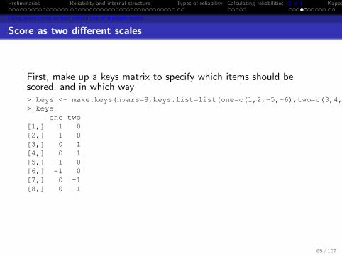
Score as two different scales
First, make up a keys matrix to specify which items should bescored, and in which way> keys <- make.keys(nvars=8,keys.list=list(one=c(1,2,-5,-6),two=c(3,4,-7,-8)))> keys
one two[1,] 1 0[2,] 1 0[3,] 0 1[4,] 0 1[5,] -1 0[6,] -1 0[7,] 0 -1[8,] 0 -1
65 / 107
Preliminaries Reliability and internal structure Types of reliability Calculating reliabilities 2 6= 1 Kappa
Using score.items to find reliabilities of multiple scales
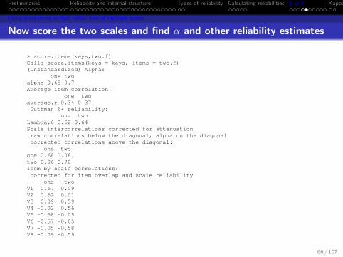
Now score the two scales and find α and other reliability estimates
> score.items(keys,two.f)Call: score.items(keys = keys, items = two.f)(Unstandardized) Alpha:
one twoalpha 0.68 0.7Average item correlation:
one twoaverage.r 0.34 0.37Guttman 6* reliability:
one twoLambda.6 0.62 0.64Scale intercorrelations corrected for attenuationraw correlations below the diagonal, alpha on the diagonalcorrected correlations above the diagonal:
one twoone 0.68 0.08two 0.06 0.70Item by scale correlations:corrected for item overlap and scale reliability
one twoV1 0.57 0.09V2 0.52 0.01V3 0.09 0.59V4 -0.02 0.56V5 -0.58 -0.05V6 -0.57 -0.05V7 -0.05 -0.58V8 -0.09 -0.59
66 / 107
Preliminaries Reliability and internal structure Types of reliability Calculating reliabilities 2 6= 1 Kappa
Intraclass correlations
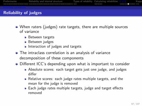
Reliability of judges
When raters (judges) rate targets, there are multiple sourcesof variance
Between targetsBetween judgesInteraction of judges and targets
The intraclass correlation is an analysis of variancedecomposition of these components
Different ICC’s depending upon what is important to consider
Absolute scores: each target gets just one judge, and judgesdifferRelative scores: each judge rates multiple targets, and themean for the judge is removedEach judge rates multiple targets, judge and target effectsremoved
67 / 107

Preliminaries Reliability and internal structure Types of reliability Calculating reliabilities 2 6= 1 Kappa
ICC of judges
Ratings of judges
What is the reliability of ratings of different judges across ratees?It depends. Depends upon the pairing of judges, depends upon thetargets. ICC does an Anova decomposition.
> RatingsJ1 J2 J3 J4 J5 J6
1 1 1 6 2 3 62 2 2 7 4 1 23 3 3 8 6 5 104 4 4 9 8 2 45 5 5 10 10 6 126 6 6 11 12 4 8
> describe(Ratings,skew=FALSE)
var n mean sd median trimmed mad min max range seJ1 1 6 3.5 1.87 3.5 3.5 2.22 1 6 5 0.76J2 2 6 3.5 1.87 3.5 3.5 2.22 1 6 5 0.76J3 3 6 8.5 1.87 8.5 8.5 2.22 6 11 5 0.76J4 4 6 7.0 3.74 7.0 7.0 4.45 2 12 10 1.53J5 5 6 3.5 1.87 3.5 3.5 2.22 1 6 5 0.76J6 6 6 7.0 3.74 7.0 7.0 4.45 2 12 10 1.53
1 1
1
1
1
1
1 2 3 4 5 6
24
68
1012
judge
Ratings
2 2
2
2
2
2
3 3
3
3
3
3
4 4
4
4
4
4
5 5
5 5
5
5
6 6
6
6
6
6
68 / 107

Preliminaries Reliability and internal structure Types of reliability Calculating reliabilities 2 6= 1 Kappa
ICC of judges
Sources of variances and the Intraclass Correlation Coefficient
Table : Sources of variances and the Intraclass Correlation Coefficient.
(J1, J2) (J3, J4) (J5, J6) (J1, J3) (J1, J5) (J1 ... J3) (J1 ... J4) (J1 ... J6)Variance estimates
MSb 7 15.75 15.75 7.0 5.2 10.50 21.88 28.33MSw 0 2.58 7.58 12.5 1.5 8.33 7.12 7.38MSj 0 6.75 36.75 75.0 0.0 50.00 38.38 30.60MSe 0 1.75 1.75 0.0 1.8 0.00 .88 2.73
Intraclass correlationsICC(1,1) 1.00 .72 .35 -.28 .55 .08 .34 .32ICC(2,1) 1.00 .73 .48 .22 .53 .30 .42 .37ICC(3,1) 1.00 .80 .80 1.00 .49 1.00 .86 .61ICC(1,k) 1.00 .84 .52 -.79 .71 .21 .67 .74ICC(2,k) 1.00 .85 .65 .36 .69 .56 .75 .78ICC(3,k) 1.00 .89 .89 1.00 .65 1.00 .96 .90
1 1
1
1
1
1
1 2 3 4 5 6
24
68
1012
judge
Ratings
2 2
2
2
2
2
3 3
3
3
3
3
4 4
4
4
4
4
5 5
5 5
5
5
6 6
6
6
6
6
69 / 107
Preliminaries Reliability and internal structure Types of reliability Calculating reliabilities 2 6= 1 Kappa
ICC of judges
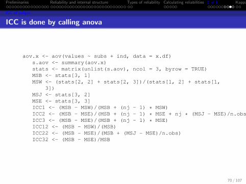
ICC is done by calling anova
aov.x <- aov(values ~ subs + ind, data = x.df)s.aov <- summary(aov.x)stats <- matrix(unlist(s.aov), ncol = 3, byrow = TRUE)MSB <- stats[3, 1]MSW <- (stats[2, 2] + stats[2, 3])/(stats[1, 2] + stats[1,
3])MSJ <- stats[3, 2]MSE <- stats[3, 3]ICC1 <- (MSB - MSW)/(MSB + (nj - 1) * MSW)ICC2 <- (MSB - MSE)/(MSB + (nj - 1) * MSE + nj * (MSJ - MSE)/n.obs)ICC3 <- (MSB - MSE)/(MSB + (nj - 1) * MSE)ICC12 <- (MSB - MSW)/(MSB)ICC22 <- (MSB - MSE)/(MSB + (MSJ - MSE)/n.obs)ICC32 <- (MSB - MSE)/MSB
70 / 107
Preliminaries Reliability and internal structure Types of reliability Calculating reliabilities 2 6= 1 Kappa
ICC of judges
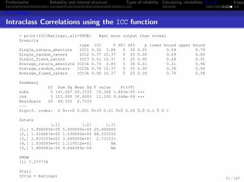
Intraclass Correlations using the ICC function
> print(ICC(Ratings),all=TRUE) #get more output than normal$results
type ICC F df1 df2 p lower bound upper boundSingle_raters_absolute ICC1 0.32 3.84 5 30 0.01 0.04 0.79Single_random_raters ICC2 0.37 10.37 5 25 0.00 0.09 0.80Single_fixed_raters ICC3 0.61 10.37 5 25 0.00 0.28 0.91Average_raters_absolute ICC1k 0.74 3.84 5 30 0.01 0.21 0.96Average_random_raters ICC2k 0.78 10.37 5 25 0.00 0.38 0.96Average_fixed_raters ICC3k 0.90 10.37 5 25 0.00 0.70 0.98
$summaryDf Sum Sq Mean Sq F value Pr(>F)
subs 5 141.667 28.3333 10.366 1.801e-05 ***ind 5 153.000 30.6000 11.195 9.644e-06 ***Residuals 25 68.333 2.7333---Signif. codes: 0 Ô***Õ 0.001 Ô**Õ 0.01 Ô*Õ 0.05 Ô.Õ 0.1 Ô Õ 1
$stats[,1] [,2] [,3]
[1,] 5.000000e+00 5.000000e+00 25.000000[2,] 1.416667e+02 1.530000e+02 68.333333[3,] 2.833333e+01 3.060000e+01 2.733333[4,] 1.036585e+01 1.119512e+01 NA[5,] 1.800581e-05 9.644359e-06 NA
$MSW[1] 7.377778
$CallICC(x = Ratings)
$n.obs[1] 6
$n.judge[1] 6
71 / 107

Preliminaries Reliability and internal structure Types of reliability Calculating reliabilities 2 6= 1 Kappa
Cohen’s kappa
Cohen’s kappa and weighted kappa
When considering agreement in diagnostic categories, withoutnumerical values, it is useful to consider the kappa coefficient.
Emphasizes matches of ratingsDoesn’t consider how far off disagreements are.
Weighted kappa weights the off diagonal distance.
Diagnostic categories: normal, neurotic, psychotic
72 / 107
Preliminaries Reliability and internal structure Types of reliability Calculating reliabilities 2 6= 1 Kappa
Weighted kappa
Cohen kappa and weighted kappa
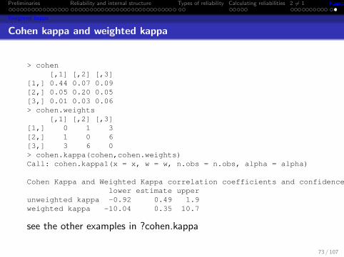
> cohen[,1] [,2] [,3]
[1,] 0.44 0.07 0.09[2,] 0.05 0.20 0.05[3,] 0.01 0.03 0.06> cohen.weights
[,1] [,2] [,3][1,] 0 1 3[2,] 1 0 6[3,] 3 6 0> cohen.kappa(cohen,cohen.weights)Call: cohen.kappa1(x = x, w = w, n.obs = n.obs, alpha = alpha)
Cohen Kappa and Weighted Kappa correlation coefficients and confidence boundarieslower estimate upper
unweighted kappa -0.92 0.49 1.9weighted kappa -10.04 0.35 10.7
see the other examples in ?cohen.kappa
73 / 107

Two approaches Various IRT models Polytomous items Factor analysis & IRT (C) A T References
Outline of Part II: the New Psychometrics
7 Two approaches
8 Various IRT models
9 Polytomous itemsOrdered response categoriesDifferential Item Functioning
10 Factor analysis & IRTNon-monotone Trace lines
11 (C) A T
74 / 107

Two approaches Various IRT models Polytomous items Factor analysis & IRT (C) A T References
Classical Reliability
1 Classical model of reliabilityObserved = True + Error
Reliability = 1− σ2error
σ2observed
Reliability = rxx = r 2xdomain
Reliability as correlation of a test with a test just like it2 Reliability requires variance in observed score
As σ2x decreases so will rxx = 1− σ2
error
σ2observed
3 Alternate estimates of reliability all share this need forvariance
1 Internal Consistency2 Alternate Form3 Test-retest4 Between rater
4 Item difficulty is ignored, items assumed to be sampled atrandom
75 / 107
Two approaches Various IRT models Polytomous items Factor analysis & IRT (C) A T References
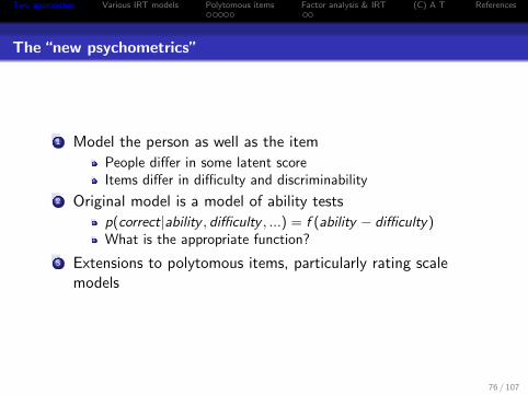
The “new psychometrics”
1 Model the person as well as the item
People differ in some latent scoreItems differ in difficulty and discriminability
2 Original model is a model of ability tests
p(correct|ability , difficulty , ...) = f (ability − difficulty)What is the appropriate function?
3 Extensions to polytomous items, particularly rating scalemodels
76 / 107
Two approaches Various IRT models Polytomous items Factor analysis & IRT (C) A T References
Classic Test Theory as 0 parameter IRT
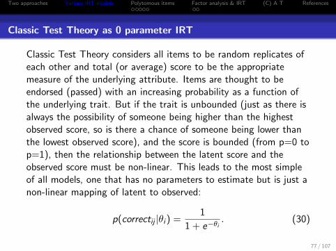
Classic Test Theory considers all items to be random replicates ofeach other and total (or average) score to be the appropriatemeasure of the underlying attribute. Items are thought to beendorsed (passed) with an increasing probability as a function ofthe underlying trait. But if the trait is unbounded (just as there isalways the possibility of someone being higher than the highestobserved score, so is there a chance of someone being lower thanthe lowest observed score), and the score is bounded (from p=0 top=1), then the relationship between the latent score and theobserved score must be non-linear. This leads to the most simpleof all models, one that has no parameters to estimate but is just anon-linear mapping of latent to observed:
p(correctij |θi ) =1
1 + e−θi. (30)
77 / 107

Two approaches Various IRT models Polytomous items Factor analysis & IRT (C) A T References
Rasch model – All items equally discriminating, differ in difficulty
Slightly more complicated than the zero parameter model is toassume that all items are equally good measures of the trait, butdiffer only in their difficulty/location. The one parameter logistic(1PL) Rasch model (Rasch, 1960) is the easiest to understand:
p(correctij |θi , δj) =1
1 + eδj−θi. (31)
That is, the probability of the i th person being correct on (orendorsing) the j th item is a logistic function of the differencebetween the person’s ability (latent trait) (θi ) and the itemdifficulty (or location) (δj). The more the person’s ability is greaterthan the item difficulty, the more likely the person is to get theitem correct.
78 / 107
Two approaches Various IRT models Polytomous items Factor analysis & IRT (C) A T References
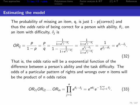
Estimating the model
The probability of missing an item, q, is just 1 - p(correct) andthus the odds ratio of being correct for a person with ability, θi , onan item with difficulty, δj is
ORij =p
1− p=
p
q=
1
1+eδj−θi
1− 1
1+eδj−θi
=
1
1+eδj−θi
eδj−θi
1+eδj−θi
=1
eδj−θi= eθi−δj .
(32)That is, the odds ratio will be a exponential function of thedifference between a person’s ability and the task difficulty. Theodds of a particular pattern of rights and wrongs over n items willbe the product of n odds ratios
ORi1ORi2 . . .ORin =n∏
j=1
eθi−δj = enθi e−∑n
j=1 δj . (33)
79 / 107
Two approaches Various IRT models Polytomous items Factor analysis & IRT (C) A T References
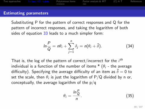
Estimating parameters
Substituting P for the pattern of correct responses and Q for thepattern of incorrect responses, and taking the logarithm of bothsides of equation 33 leads to a much simpler form:
lnP
Q= nθi +
n∑j=1
δj = n(θi + δ̄). (34)
That is, the log of the pattern of correct/incorrect for the i th
individual is a function of the number of items * (θi - the averagedifficulty). Specifying the average difficulty of an item as δ̄ = 0 toset the scale, then θi is just the logarithm of P/Q divided by n or,conceptually, the average logarithm of the p/q
θi =ln P
Q
n. (35)
80 / 107
Two approaches Various IRT models Polytomous items Factor analysis & IRT (C) A T References
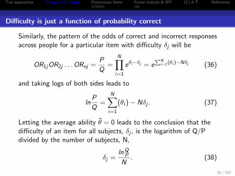
Difficulty is just a function of probability correct
Similarly, the pattern of the odds of correct and incorrect responsesacross people for a particular item with difficulty δj will be
OR1jOR2j . . .ORnj =P
Q=
N∏i=1
eθi−δj = e∑N
i=1(θi )−Nδj (36)
and taking logs of both sides leads to
lnP
Q=
N∑i=1
(θi )− Nδj . (37)
Letting the average ability θ̄ = 0 leads to the conclusion that thedifficulty of an item for all subjects, δj , is the logarithm of Q/Pdivided by the number of subjects, N,
δj =lnQ
P
N. (38)
81 / 107

Two approaches Various IRT models Polytomous items Factor analysis & IRT (C) A T References
Rasch model in words
That is, the estimate of ability (Equation 35) for items with anaverage difficulty of 0 does not require knowing the difficulty ofany particular item, but is just a function of the pattern of correctsand incorrects for a subject across all items.Similarly, the estimate of item difficulty across people ranging inability, but with an average ability of 0 (Equation 38) is a functionof the response pattern of all the subjects on that one item anddoes not depend upon knowing any one person’s ability. Theassumptions that average difficulty and average ability are 0 aremerely to fix the scales. Replacing the average values with anon-zero value just adds a constant to the estimates.
82 / 107
Two approaches Various IRT models Polytomous items Factor analysis & IRT (C) A T References
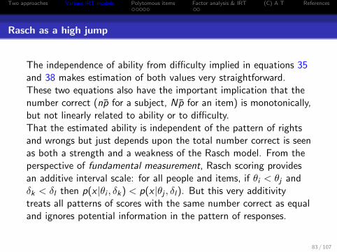
Rasch as a high jump
The independence of ability from difficulty implied in equations 35and 38 makes estimation of both values very straightforward.These two equations also have the important implication that thenumber correct (np̄ for a subject, Np̄ for an item) is monotonically,but not linearly related to ability or to difficulty.That the estimated ability is independent of the pattern of rightsand wrongs but just depends upon the total number correct is seenas both a strength and a weakness of the Rasch model. From theperspective of fundamental measurement, Rasch scoring providesan additive interval scale: for all people and items, if θi < θj andδk < δl then p(x |θi , δk) < p(x |θj , δl). But this very additivitytreats all patterns of scores with the same number correct as equaland ignores potential information in the pattern of responses.
83 / 107
Two approaches Various IRT models Polytomous items Factor analysis & IRT (C) A T References
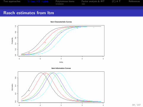
Rasch estimates from ltm
-4 -2 0 2 4
0.0
0.2
0.4
0.6
0.8
1.0
Item Characteristic Curves
Ability
Probability
Q1
Q5
Q4
Q2 Q3
-4 -2 0 2 4
0.0
0.2
0.4
0.6
Item Information Curves
Ability
Information
Q1
Q5
Q4
Q2
Q3
-2 -1 0 1
0.0
0.1
0.2
0.3
0.4
0.5
0.6
Kernel Density Estimation for Ability Estimates
Ability
Density
84 / 107

Two approaches Various IRT models Polytomous items Factor analysis & IRT (C) A T References
The LSAT example from ltm
data(bock)> ord <- order(colMeans(lsat6),decreasing=TRUE)> lsat6.sorted <- lsat6[,ord]> describe(lsat6.sorted)> Tau <- round(-qnorm(colMeans(lsat6.sorted)),2) #tau = estimates of threshold> rasch(lsat6.sorted,constraint=cbind(ncol(lsat6.sorted)+1,1.702))
var n mean sd median trimmed mad min max range skew kurtosis seQ1 1 1000 0.92 0.27 1 1.00 0 0 1 1 -3.20 8.22 0.01Q5 2 1000 0.87 0.34 1 0.96 0 0 1 1 -2.20 2.83 0.01Q4 3 1000 0.76 0.43 1 0.83 0 0 1 1 -1.24 -0.48 0.01Q2 4 1000 0.71 0.45 1 0.76 0 0 1 1 -0.92 -1.16 0.01Q3 5 1000 0.55 0.50 1 0.57 0 0 1 1 -0.21 -1.96 0.02
> TauQ1 Q5 Q4 Q2 Q3
-1.43 -1.13 -0.72 -0.55 -0.13
Call:rasch(data = lsat6.sorted, constraint = cbind(ncol(lsat6.sorted) +
1, 1.702))
Coefficients:Dffclt.Q1 Dffclt.Q5 Dffclt.Q4 Dffclt.Q2 Dffclt.Q3 Dscrmn
-1.927 -1.507 -0.960 -0.742 -0.195 1.702
85 / 107

Two approaches Various IRT models Polytomous items Factor analysis & IRT (C) A T References
Item information
When forming a test and evaluating the items within a test, themost useful items are the ones that give the most informationabout a person’s score. In classic test theory, item information isthe reciprocal of the squared standard error for the item or for aone factor test, the ratio of the item communality to its uniqueness:
Ij =1
σ2ej
=h2j
1− h2j
.
When estimating ability using IRT, the information for an item is afunction of the first derivative of the likelihood function and ismaximized at the inflection point of the icc.
86 / 107
Two approaches Various IRT models Polytomous items Factor analysis & IRT (C) A T References
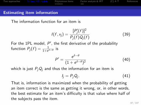
Estimating item information
The information function for an item is
I (f , xj) =[P ′j (f )]2
Pj(f )Qj(f )(39)
For the 1PL model, P ′, the first derivative of the probabilityfunction Pj(f ) = 1
1+eδ−θis
P ′ =eδ−θ
(1 + eδ−θ)2(40)
which is just PjQj and thus the information for an item is
Ij = PjQj . (41)
That is, information is maximized when the probability of gettingan item correct is the same as getting it wrong, or, in other words,the best estimate for an item’s difficulty is that value where half ofthe subjects pass the item.
87 / 107
Two approaches Various IRT models Polytomous items Factor analysis & IRT (C) A T References
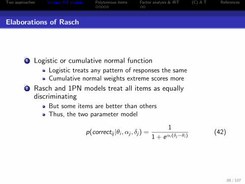
Elaborations of Rasch
1 Logistic or cumulative normal function
Logistic treats any pattern of responses the sameCumulative normal weights extreme scores more
2 Rasch and 1PN models treat all items as equallydiscriminating
But some items are better than othersThus, the two parameter model
p(correctij |θi , αj , δj) =1
1 + eαi (δj−θi )(42)
88 / 107

Two approaches Various IRT models Polytomous items Factor analysis & IRT (C) A T References
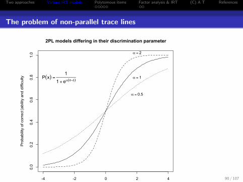
2PL and 2PN models
p(correctij |θi , αj , δj) =1
1 + eαi (δj−θi )(43)
while in the two parameter normal ogive (2PN) model this is
p(correct|θ, αj , δ) =1√2π
∫ α(θ−δ)
− infe−
u2
2 du (44)
where u = α(θ − δ).The information function for a two parameter model reflects theitem discrimination parameter, α,
Ij = α2PjQj (45)
which, for a 2PL model is
Ij = α2j PjQj =
α2j
(1 + eαj (δj−θj ))2. (46)
89 / 107
Two approaches Various IRT models Polytomous items Factor analysis & IRT (C) A T References
The problem of non-parallel trace lines
-4 -2 0 2 4
0.0
0.2
0.4
0.6
0.8
1.0
2PL models differing in their discrimination parameter
Ability (logit units)
Pro
babi
lity
of c
orre
ct |a
bilit
y an
d di
fficu
lty
α = 0.5
α = 1
α = 2
P(x) =1
1 + eα(θ−δ)
90 / 107
Two approaches Various IRT models Polytomous items Factor analysis & IRT (C) A T References
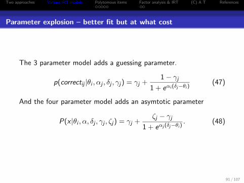
Parameter explosion – better fit but at what cost
The 3 parameter model adds a guessing parameter.
p(correctij |θi , αj , δj , γj) = γj +1− γj
1 + eαi (δj−θi )(47)
And the four parameter model adds an asymtotic parameter
P(x |θi , α, δj , γj , ζj) = γj +ζj − γj
1 + eαj (δj−θi ). (48)
91 / 107

Two approaches Various IRT models Polytomous items Factor analysis & IRT (C) A T References
frame
-4 -2 0 2 4
0.0
0.4
0.8
3PL models differing in guessing and difficulty
Ability in logit unitsPro
babi
lity
of c
orre
ct |a
bilit
y an
d di
fficu
lty
γ = 0 δ = 0γ = 0.2 δ = 1
γ = 0.2 δ = −1γ = 0.3 δ = 0
P(x) = γ +1 − γ
1 + eα(θ−δ)
-4 -2 0 2 4
0.0
0.4
0.8
4PL items differing in guessing, difficulty and asymptote
Ability in logit unitsPro
babi
lity
of c
orre
ct |a
bilit
y an
d di
fficu
lty
γ = 0 δ = 0γ = 0.2 δ = 1
γ = 0.2 ζ = 0.8
γ = 0.2 δ = −1
P(x) = γ +ζ − γ
1 + eα(θ−δ)
92 / 107

Two approaches Various IRT models Polytomous items Factor analysis & IRT (C) A T References
Ordered response categories
Personality items with monotone trace lines
A typical personality item might ask “How much do you enjoy alively party” with a five point response scale ranging from “1: notat all” to “5: a great deal” with a neutral category at 3. Analternative response scale for this kind of item is to not have aneutral category but rather have an even number of responses.Thus a six point scale could range from “1: very inaccurate” to “6:very accurate” with no neutral categoryThe assumption is that the more sociable one is, the higher theresponse alternative chosen. The probability of endorsing a 1 willincrease monotonically the less sociable one is, the probability ofendorsing a 5 will increase monotonically the more sociable one is.
93 / 107
Two approaches Various IRT models Polytomous items Factor analysis & IRT (C) A T References
Ordered response categories
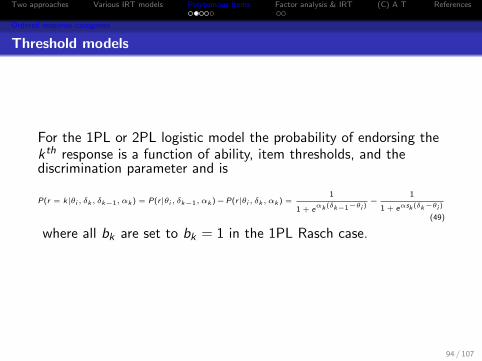
Threshold models
For the 1PL or 2PL logistic model the probability of endorsing thekth response is a function of ability, item thresholds, and thediscrimination parameter and is
P(r = k|θi , δk , δk−1, αk ) = P(r|θi , δk−1, αk )−P(r|θi , δk , αk ) =1
1 + eαk (δk−1−θi )
−1
1 + eαsk (δk−θi )
(49)
where all bk are set to bk = 1 in the 1PL Rasch case.
94 / 107
Two approaches Various IRT models Polytomous items Factor analysis & IRT (C) A T References
Ordered response categories
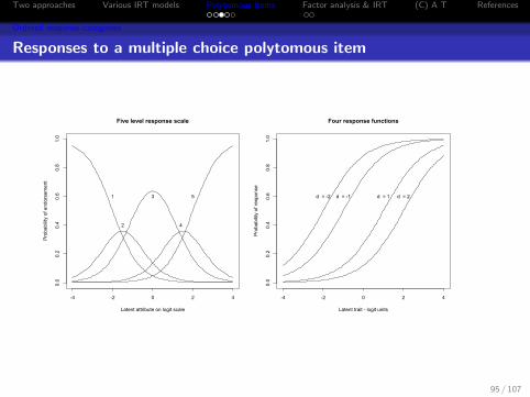
Responses to a multiple choice polytomous item
-4 -2 0 2 4
0.0
0.2
0.4
0.6
0.8
1.0
Five level response scale
Latent attribute on logit scale
Pro
babi
lity
of e
ndor
sem
ent
1
2
3
4
5
-4 -2 0 2 4
0.0
0.2
0.4
0.6
0.8
1.0
Four response functions
Latent trait - logit units
Pro
babi
lity
of re
spon
se
d = -2 d = -1 d = 1 d = 2
95 / 107
Two approaches Various IRT models Polytomous items Factor analysis & IRT (C) A T References
Ordered response categories
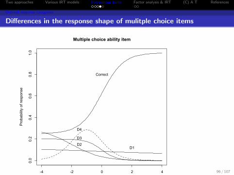
Differences in the response shape of mulitple choice items
-4 -2 0 2 4
0.0
0.2
0.4
0.6
0.8
1.0
Multiple choice ability item
Ability in logit units
Pro
babi
lity
of re
spon
se
Correct
D1D2
D3
D4
96 / 107

Two approaches Various IRT models Polytomous items Factor analysis & IRT (C) A T References
Differential Item Functioning
Differential Item Functioning
1 Use of IRT to analyze item quality
Find IRT difficulty and discrimination parameters for differentgroupsCompare response patterns
-3 -2 -1 0 1 2 3
0.0
0.2
0.4
0.6
0.8
1.0
Differential Item Functioning
θ
Pro
babi
lity
of R
espo
nse
MalesFemales
97 / 107
Two approaches Various IRT models Polytomous items Factor analysis & IRT (C) A T References
FA and IRT
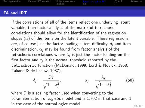
If the correlations of all of the items reflect one underlying latentvariable, then factor analysis of the matrix of tetrachoriccorrelations should allow for the identification of the regressionslopes (α) of the items on the latent variable. These regressionsare, of course just the factor loadings. Item difficulty, δj and itemdiscrimination, αj may be found from factor analysis of thetetrachoric correlations where λj is just the factor loading on thefirst factor and τj is the normal threshold reported by thetetrachoric function (McDonald, 1999; Lord & Novick, 1968;Takane & de Leeuw, 1987).
δj =Dτ√1− λ2
j
, αj =λj√
1− λ2j
(50)
where D is a scaling factor used when converting to theparameterization of logistic model and is 1.702 in that case and 1in the case of the normal ogive model.
98 / 107

Two approaches Various IRT models Polytomous items Factor analysis & IRT (C) A T References
FA and IRT
IRT parameters from FA
δj =Dτ√1− λ2
j
, αj =λj√
1− λ2j
(51)
FA parameters from IRT
λj =αj√
1 + α2j
, τj =δj√
1 + α2j
.
99 / 107
Two approaches Various IRT models Polytomous items Factor analysis & IRT (C) A T References
the irt.fa function
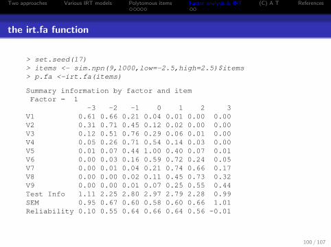
> set.seed(17)> items <- sim.npn(9,1000,low=-2.5,high=2.5)$items> p.fa <-irt.fa(items)
Summary information by factor and itemFactor = 1
-3 -2 -1 0 1 2 3V1 0.61 0.66 0.21 0.04 0.01 0.00 0.00V2 0.31 0.71 0.45 0.12 0.02 0.00 0.00V3 0.12 0.51 0.76 0.29 0.06 0.01 0.00V4 0.05 0.26 0.71 0.54 0.14 0.03 0.00V5 0.01 0.07 0.44 1.00 0.40 0.07 0.01V6 0.00 0.03 0.16 0.59 0.72 0.24 0.05V7 0.00 0.01 0.04 0.21 0.74 0.66 0.17V8 0.00 0.00 0.02 0.11 0.45 0.73 0.32V9 0.00 0.00 0.01 0.07 0.25 0.55 0.44Test Info 1.11 2.25 2.80 2.97 2.79 2.28 0.99SEM 0.95 0.67 0.60 0.58 0.60 0.66 1.01Reliability 0.10 0.55 0.64 0.66 0.64 0.56 -0.01
100 / 107

Two approaches Various IRT models Polytomous items Factor analysis & IRT (C) A T References
Item Characteristic Curves from FA
-3 -2 -1 0 1 2 3
0.0
0.2
0.4
0.6
0.8
1.0
Item parameters from factor analysis
Latent Trait (normal scale)
Pro
babi
lity
of R
espo
nse
1 2 3 4 5 6 7 8 9
101 / 107
Two approaches Various IRT models Polytomous items Factor analysis & IRT (C) A T References
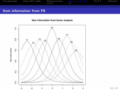
Item information from FA
-3 -2 -1 0 1 2 3
0.0
0.2
0.4
0.6
0.8
1.0
Item information from factor analysis
Latent Trait (normal scale)
Item
Info
rmat
ion
V1V2
V3 V4
V5
V6
V7
V8
V9
102 / 107
Two approaches Various IRT models Polytomous items Factor analysis & IRT (C) A T References
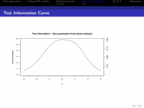
Test Information Curve
-3 -2 -1 0 1 2 3
01
23
45
6
Test information -- item parameters from factor analysis
x
Test
Info
rmat
ion
0.31
0.66
0.77
0.83
103 / 107

Two approaches Various IRT models Polytomous items Factor analysis & IRT (C) A T References
Comparing three ways of estimating the parameters
set.seed(17)items <- sim.npn(9,1000,low=-2.5,high=2.5)$itemsp.fa <- irt.fa(items)$coefficients[1:2]p.ltm <- ltm(items~z1)$coefficientsp.ra <- rasch(items, constraint = cbind(ncol(items) + 1, 1))$coefficientsa <- seq(-2.5,2.5,5/8)p.df <- data.frame(a,p.fa,p.ltm,p.ra)round(p.df,2)
a Difficulty Discrimination X.Intercept. z1 beta.i betaItem 1 -2.50 -2.45 1.03 5.42 2.61 3.64 1Item 2 -1.88 -1.84 1.00 3.35 1.88 2.70 1Item 3 -1.25 -1.22 1.04 2.09 1.77 1.73 1Item 4 -0.62 -0.69 1.03 1.17 1.71 0.98 1Item 5 0.00 -0.03 1.18 0.04 1.94 0.03 1Item 6 0.62 0.63 1.05 -1.05 1.68 -0.88 1Item 7 1.25 1.43 1.10 -2.47 1.90 -1.97 1Item 8 1.88 1.85 1.01 -3.75 2.27 -2.71 1Item 9 2.50 2.31 0.90 -5.03 2.31 -3.66 1
104 / 107

Two approaches Various IRT models Polytomous items Factor analysis & IRT (C) A T References
Non-monotone Trace lines
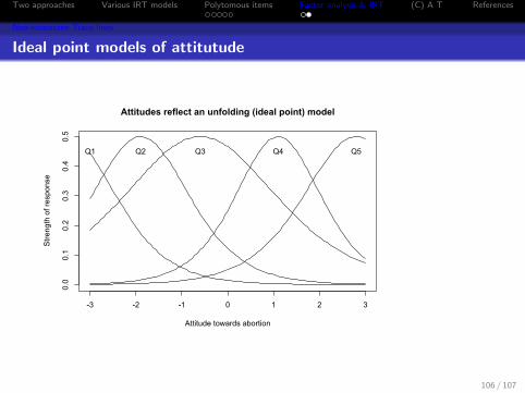
Attitudes might not have monotone trace lines
1 Abortion is unacceptable under any circumstances.2 Even if one believes that there may be some
exceptions, abortions is still generally wrong.3 There are some clear situations where abortion
should be legal, but it should not be permitted in allsituations.
4 Although abortion on demand seems quite extreme,I generally favor a woman’s right to choose.
5 Abortion should be legal under any circumstances.
105 / 107
Two approaches Various IRT models Polytomous items Factor analysis & IRT (C) A T References
Non-monotone Trace lines
Ideal point models of attitutude
-3 -2 -1 0 1 2 3
0.0
0.1
0.2
0.3
0.4
0.5
Attitude towards abortion
Stre
ngth
of r
espo
nse
Q1 Q2 Q3 Q4 Q5
Attitudes reflect an unfolding (ideal point) model
106 / 107
Two approaches Various IRT models Polytomous items Factor analysis & IRT (C) A T References
IRT and CTT don’t really differ except
1 Correlation of classic test scores and IRT scores > .98.
2 Test information for the person doesnt’t require people to vary3 Possible to item bank with IRT
Make up tests with parallel items based upon difficulty anddiscriminationDetect poor items
4 Adaptive testing
No need to give a person an item that they will almostcertainly pass (or fail)Can tailor the test to the person(Problem with anxiety and item failure)
107 / 107
Two approaches Various IRT models Polytomous items Factor analysis & IRT (C) A T References
Lord, F. M. & Novick, M. R. (1968). Statistical theories of mentaltest scores. The Addison-Wesley series in behavioral science:quantitative methods. Reading, Mass.: Addison-Wesley Pub. Co.
McDonald, R. P. (1999). Test theory: A unified treatment.Mahwah, N.J.: L. Erlbaum Associates.
Rasch, G. (1960). Probabilistic models for some intelligence andattainment tests. Chicago: reprinted in 1980 by The Universityof Chicago Press /Paedagogike Institut, Copenhagen.
Spearman, C. (1904). The proof and measurement of associationbetween two things. The American Journal of Psychology,15(1), 72–101.
Takane, Y. & de Leeuw, J. (1987). On the relationship betweenitem response theory and factor analysis of discretized variables.Psychometrika, 52, 393–408. 10.1007/BF02294363.
107 / 107