us housing since 2001 · 2017-02-15 · miami var prices rhpi rhpig rhping ... and mortgage rates...
TRANSCRIPT

US Housing since 2001:
What’s different this time?
William Wheaton
Department of Economics
Center for Real Estate
MIT
January, 2017
IAP
HISTORIC PERSPECTIVE: WHAT HAS HAPPENED TO REAL PRICES AND UNIT CONSTRUCTION: 1981-2016
1). - 68 Markets = 68 stories?
- Coastal cities
- Mid West Hinterland
- Sunbelt
2). What to look at?
- Housing prices (constant dollars, FHA repeat sale price index)
- New construction: total building permits
- Long term trends in each
- Recession volatility: historic –vs- 2001/2016
(Ignore Green/Blue)

Coastal markets: Boston
Boston
VAR prices
RHPI RHPIG RHPING
1980 1985 1990 1995 2000 2005 2010 2015
100
150
200
250
300
350
VAR permits
1980 1985 1990 1995 2000 2005 2010 2015
0
2000
4000
6000
8000
10000
12000PRM
PRMG
PRMNG

Coastal markets: LA
LosAngeles
VAR prices
RHPI RHPIG RHPING
1980 1985 1990 1995 2000 2005 2010 2015
100
150
200
250
300
350
400
VAR permits
1980 1985 1990 1995 2000 2005 2010 2015
0
2500
5000
7500
10000
12500
15000
17500
20000PRM
PRMG
PRMNG
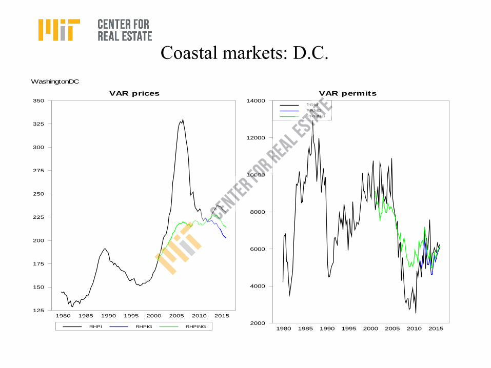
Coastal markets: D.C.
WashingtonDC
VAR prices
RHPI RHPIG RHPING
1980 1985 1990 1995 2000 2005 2010 2015125
150
175
200
225
250
275
300
325
350
VAR permits
1980 1985 1990 1995 2000 2005 2010 20152000
4000
6000
8000
10000
12000
14000PRM
PRMG
PRMNG
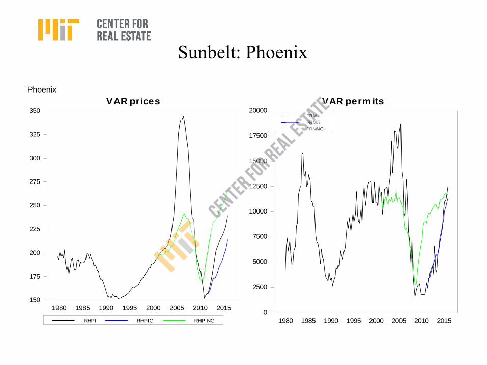
Sunbelt: Phoenix
Phoenix
VAR prices
RHPI RHPIG RHPING
1980 1985 1990 1995 2000 2005 2010 2015
150
175
200
225
250
275
300
325
350
VAR permits
1980 1985 1990 1995 2000 2005 2010 2015
0
2500
5000
7500
10000
12500
15000
17500
20000PRM
PRMG
PRMNG

Sunbelt markets: Miami
Miami
VAR prices
RHPI RHPIG RHPING
1980 1985 1990 1995 2000 2005 2010 2015
100
150
200
250
300
350
400
VAR permits
1980 1985 1990 1995 2000 2005 2010 2015
0
2500
5000
7500
10000PRM
PRMG
PRMNG

Sunbelt markets: Atlanta
Atlanta
VAR prices
RHPI RHPIG RHPING
1980 1985 1990 1995 2000 2005 2010 2015130
140
150
160
170
180
190
200
210
220
VAR permits
1980 1985 1990 1995 2000 2005 2010 20150
2500
5000
7500
10000
12500
15000
17500
20000
22500PRM
PRMG
PRMNG

Midwest markets: Chicago
Chicago
VAR prices
RHPI RHPIG RHPING
1980 1985 1990 1995 2000 2005 2010 2015
100
120
140
160
180
200
220
240
260
VAR permits
1980 1985 1990 1995 2000 2005 2010 2015
0
2000
4000
6000
8000
10000
12000
14000PRM
PRMG
PRMNG

Midwest markets: St. Louis
StLouis
VAR prices
RHPI RHPIG RHPING
1980 1985 1990 1995 2000 2005 2010 2015
140
150
160
170
180
190
200
210
220
VAR permits
1980 1985 1990 1995 2000 2005 2010 2015
500
1000
1500
2000
2500
3000
3500
4000
4500
5000PRM
PRMG
PRMNG

Midwest markets: Kansas City
KansasCity
VAR prices
RHPI RHPIG RHPING
1980 1985 1990 1995 2000 2005 2010 2015150
160
170
180
190
200
210
VAR permits
1980 1985 1990 1995 2000 2005 2010 20150
1000
2000
3000
4000
5000PRM
PRMG
PRMNG

HISTORIC PERSPECTIVE: WHAT HAS HAPPENED TO REAL PRICES AND UNIT CONSTRUCTION: 1981-2016
1). - Strong upward trend in constant $ house prices on the coasts.
- 2001-2011 Volatility greater than past recessions
2). - Much less (or no) price trend in Mid West
- 2001-2011 volatility still much greater.
3). - Little or no price trend in the Sunbelt.
- 2001-2011 volatility enormous, dominating
4). - In all markets, the trend in unit construction is
flat or downward (slower demographic growth?)
- Construction I(0) moves closest with price
levels I(1)

BUT 2001-2016 INCLUDED:
(1) A STRONG ECONOMIC RECOVERY (2001-2006)
(2) THE WORST RECESSION SINCE 1930.
HOW MUCH VOLATILITY IS EXPLAINED BY THOSE?
1). - Estimate a VAR model with house price growth and new construction (both variables stationary)
2). - Make the VAR conditional on local job growth and Mortgage rates (the 2 most important economic drivers of housing in the literature).
3). - # lags (SBIC test) generally 5-7.
4). - Back test: Use the model to dynamically forecast prices and construction, beginning in 2001 and extending to 2016 – using actual employment growth and mortgage rates in each market. (green line).
Repeat for recovery starting in 2011 (blue line).

Phoenix VAR forecast Errors in price changes: Phoenix
VAR prices
RHPI RHPIG RHPING
1980 1985 1990 1995 2000 2005 2010 2015
150
175
200
225
250
275
300
325
350
VAR permits
1980 1985 1990 1995 2000 2005 2010 2015
0
2500
5000
7500
10000
12500
15000
17500
20000PRM
PRMG
PRMNG

RESULTS1). - In all markets forecast prices rise upward (at bit)
from 2001 to 2006 as local economies improve from the 2001 recession. On average the forecast rise is 8% versus an actual rise of 41%!
2). - In virtually all markets forecast prices drop from 2007 to 2011, but on average by only 5% as a sharp drop in mortgage rates help cushion that impact of severe job losses. The actual drop is 42%!
3). - From 2011 to today forecast prices rise an average 10% as opposed to a 12% actual recovery.
4). - Construction errors tend to follow price errors
5). - Forecast 2016 price levels on average are 14% ahead of 2001, actual are 11%.
The forecast misses all the volatility: the “Bubble”

Question #1: where is the “bubble” biggestAbsolute value forecast error: |2006-2001| + |2011-2006|
Largest Smallest
Miami 2.18429
LosAngeles 2.02762
FortLauderdale1.81099
Orlando 1.6072
WestPalmBeach1.42981
LasVegas 1.36861
Tampa 1.33156
Tucson 1.32317
Phoenix 1.2671
OrangeCounty1.25254
SanDiego 1.24643
Ventura 1.20361
Dallas 0.23586
FortWorth 0.22419
Cleveland 0.19361
Buffalo 0.185464
Tulsa 0.17275
Raleigh 0.16647
Cincinnati 0.16511
Columbus 0.16302
Greensboro 0.16022
Louisville 0.15486
Dayton 0.14657
Pittsburgh 0.12142
Indianapolis0.04112
(“CANFLAZ”)

Hypothesis #1: purchase of 2nd or Investment (speculative)
homes fed demand (Condos excluded)
Source: Loan Performance, Torto Wheaton Research
0 10 20 30 40 50
Nation
San Diego
Sacramento
Riverside
Miami
Tampa
Phoenix
Orlando
Las Vegas
Fort Myers
Atlantic City
1999
2005
Investment and 2nd Home Loans as Share of New Loans, %

The simple statistics are suggestive: prices appreciate
more where second home buying is on the rise.
y = 0.0273x + 14.536
R2 = 0.4201
0
20
40
60
80
100
-1,000 0 1,000 2,000 3,000
2002-2005 cumulative change in shares
of investment and 2nd home loans, BPS
2002-2005 Cumulative change in HPI, %
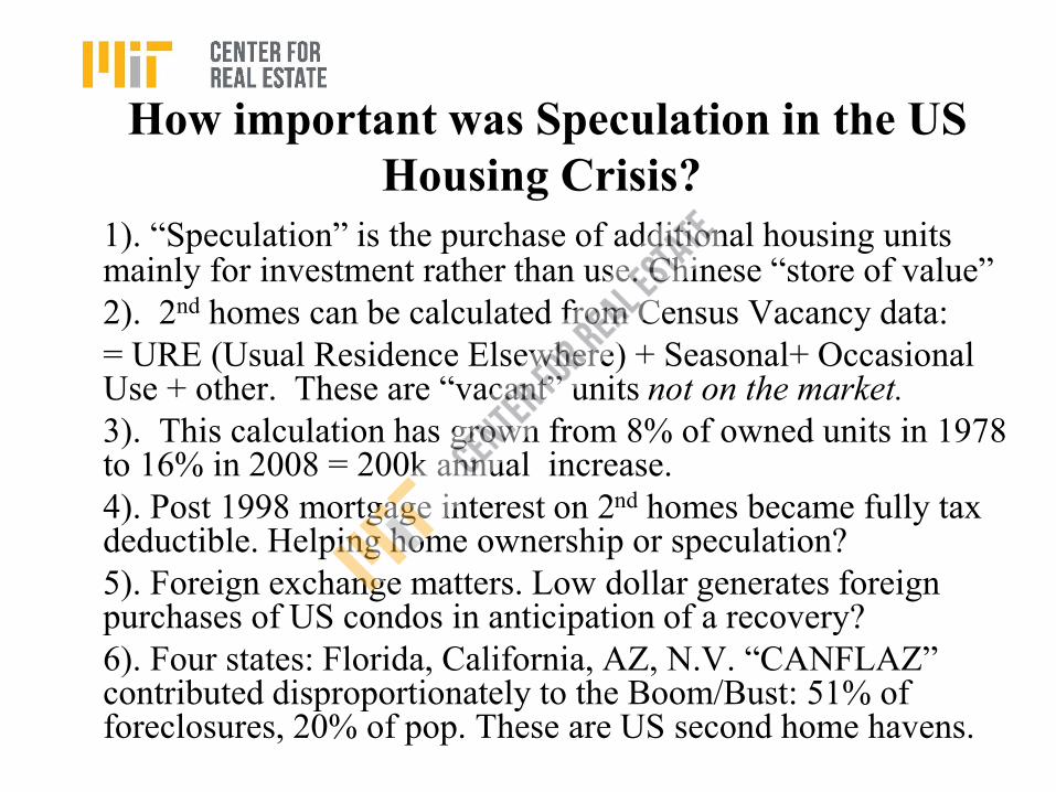
How important was Speculation in the US
Housing Crisis?
1). “Speculation” is the purchase of additional housing units mainly for investment rather than use. Chinese “store of value”
2). 2nd homes can be calculated from Census Vacancy data:
= URE (Usual Residence Elsewhere) + Seasonal+ Occasional Use + other. These are “vacant” units not on the market.
3). This calculation has grown from 8% of owned units in 1978 to 16% in 2008 = 200k annual increase.
4). Post 1998 mortgage interest on 2nd homes became fully tax deductible. Helping home ownership or speculation?
5). Foreign exchange matters. Low dollar generates foreign purchases of US condos in anticipation of a recovery?
6). Four states: Florida, California, AZ, N.V. “CANFLAZ” contributed disproportionately to the Boom/Bust: 51% of foreclosures, 20% of pop. These are US second home havens.

But 1996-2007 “Bubble” and subsequent “bust” also mirrored
an unprecedented rise/fall in home ownership. Did the Rising
ownership share fuel house prices or reverse?

The ownership – Price nexus
• High house price levels make ownership less
affordable, but rising prices lower the annual
cost of owning, stimulating ownership.
• Low house prices makes houses affordable, but
falling house prices generate strategic defaults,
foreclosures, falling ownership.
• Willen (2016). Increase in ownership rate up to
2007 occurred almost uniformly across all
income groups! Not a low income phenomena.
• Did it rise equally in all locations?

CANFLAZ homeownership rose/fell 2x US!
(But state/local ownership data too thin for further
analysis)
60
61
62
63
64
65
66
67
68
69
70
199
1
199
2
199
3
199
4
199
5
199
6
199
7
199
8
199
9
200
0
200
1
200
2
200
3
200
4
200
5
200
6
200
7
200
8
200
9
201
0
201
1
US CANVFLAZ (simple average)
Homeownership rate, %

Hypothesis #2: Homeownership movement suggests
Credit “availability” expanded/contracted (LTV, DTI,
documentation requirements...)
0
100
200
300
400
500
600
700
1994 1995 1996 1997 1998 1999 2000 2001 2002 2003 2004 2005
0
4
8
12
16
20
24
28
Subprime Loan Origiations
Subprime as % of Total Originations
Subprime Originations as % Total Mortgage Debt Outstanding
$ Billions Percent

Evidence of credit relaxation in
the conforming loan market
• Fraction of conforming home purchase loans with
LTV>80%: 1998 (55%),2004 (65%), 2009 (72%).
• Fraction of conforming home purchase loans with
DTI>40%: 1998 (25%), 2004 (40%), 2009 (40%).
• Subprime loan market has loans with credit
standards way below the conforming market and
its market share rose significantly until it
collapsed in 2008.

What about the recovery since 2011?
• On average prices have increased 12% (constant
dollars) 22% in current dollars since 2011.
• The 2001 back test forecast predicted 10%
(constant $) recovery. Pretty close
• A back test from 2011 predicted 9% also not bad
• Job growth and continued low rates over the last 5
years well predicts the house price recovery so far
• Looking beyond 2016, what will happen to jobs
and rates? And then what is the model missing?

Since 2012: A once-in-a-lifetime opportunity! But
future Rents fall (new construction) and rates will rise
Negative factors for a post 2016 model forecast
3.0
4.5
6.0
7.5
9.0
10.5
12.0
13.5
0.8
1.0
1.2
1.4
1.6
1.8
2.0
2.2
19
86
19
87
19
88
19
89
19
90
19
91
19
92
19
93
19
94
19
95
19
96
19
97
19
98
19
99
20
00
20
01
20
02
20
03
20
04
20
05
20
06
20
07
20
08
20
09
20
10
20
11
20
12
20
13
P/R and i*P/R Ratios, 2013q2=1 30-year fixed mortgage rate, %
P/R ratio
i*P/R ratio
Mortgage rate
Sources: BLS, FHFA, CBRE EA.

Housing starts have been way below household formation
and total demand (+ 2nd homes & demolitions) for 8 years.
Inevitable construction recovery also limits future prices
1997-2008
6.5 Mil
Historic Equilibrium: 222,000 excess units (=demolitions + second homes )

Future Job growth contrained • Job growth is increasingly constrained post 2016
– Aging means a labor force that grows at less than 1%
yearly (<100k new jobs/month becomes the new
steady state, full employment normal)
– The prospect of Immigration reform limits job
growth significantly from farm workers to H1B
programmers.
– As we near full a employment rate (95.2%) these
factors dominate the cyclic changes in labor force
participation.
– Limit further price recovery

What about household formation?
• Household formation from 2008-2016 is only
65% of what it was prior to the Recession.
– Huge increase in millennials (age 20-35) living at
home (27% in 2010 versus 15% in 1980).
– Increase in doubling up (economic hardship and
rising rents)
– This despite: increases in divorce, singledom and
aging (all boost headship rates, FRB study)
– Household formation data is difficult nationally
and non-existent at local market level.
Outside the model

…and home ownership?
• Home Ownership fallen almost 6% since 2007
• Permanent change in tenure “preference”, fear of
asset loss, love of no commitment, job insecurity?
• Millennials never married rate soared to 62%
from 32% (1980). Singles rent.
• Extreme foreclosures, households left with no
equity after recession so moving requires renting.
• “Outside the model” because difficult to get local
market data on ownership

1). A recovery in Household Formation
- 2000-2007 Household formation averages: 1,285,000 yearly
- From 2008-2015 averages: 780,000
- It has to return to 1,200,000 range plus make up for lost formation of 2m during the downturn!
- Economists in accord that it will recover
2). A permanent shift in ownership/tenure choice?
- Credit standards are relaxing again, mortgages
available with greater flexibility.
- Wages finally starting to improve.
- Unique opportunity argument.
- Millennial issues are temporary, postponing
- They will shortly grow up, marry, move, buy.
Future Prospects

345678910111213141516
1986
1987
1988
1989
1990
1991
1992
1993
1994
1995
1996
1997
1998
1999
2000
2001
2002
2003
2004
2005
2006
2007
2008
2009
2010
2011
2012
2013
2014
2015
Delinquency Rate Transition to foreclosureSource: Mortgage Bankers Association
Mortgage Delinquency leveling off, foreclosures
dropping, recovering equity… all positive

Factors outside model all look positive: household
formation recovers, renter growth declines, # owners surge

Conclusions• Boom/Bust largely unexplained by economic fundamentals
• But post 2011 recovery in prices and Housing construction is well explained by job growth and mortgage rates.
• Future outlook for job growth and rates is all negative.
• Price growth in all markets has recovered to or above pre-boom 2001 levels (constant $), but model forecast beyond 2016 should have price growth slowing – so a long way back to 2007 peak price levels (never?).
• Factors outside of the model, however, generally support stronger price growth: – Pick up/recovery in household formation
– Stabilizing, reviving home ownership rate
– Reductions in negative equity restore mobility
• What have I left out?

Conclusions• Real prices back to or ahead of 2001.
• Long way to go to be back to 2007 levels
• then again if real interest rates rise