Valuation of Mortgage-Backed Securities and

Mortgage Derivatives: A Closed-Form

Approximation

Andreas Kolbe ∗† Rudi Zagst ‡

May 16, 2007

Abstract

In this paper we develop a closed-form and thus computationally highlyefficient formula to approximate the value of fixed-rate MBS. Our mod-elling framework is based on reduced-form and prepayment-risk neu-tral valuation techniques and offers two major extensions comparedto existing closed-form approximation approaches: We are not limitedto one stochastic factor and we are able to capture the usual S-curveshape of the refinancing incentive by a piecewise linear approximation.We apply our model to a sample of GNMA pass-through securities andfind that our model is able to explain market price movements with ahighly satisfactory accuracy for a wide range of coupons.

Keywords: mortgage-backed security, prepayment, closed-form, risk-neutral pricing

JEL classification: G12, G13

∗HVB-Institute for Mathematical Finance, Munich University of Technology, Boltz-mannstr. 3, D-85748 Garching (Munich), Germany, kolbe@ma.tum.de

†Support from Bayerische Landesbank (BayernLB), Risk Control Trading Sections,Munich and BayernLB Risk Control Americas, New York, is gratefully acknowledged

‡HVB-Institute for Mathematical Finance, Munich University of Technology, Boltz-mannstr. 3, D-85748 Garching (Munich), Germany, zagst@ma.tum.de

1

1 Introduction

The valuation of mortgage-backed securities is usually considered a compu-tationally expensive problem. This holds for both categories of valuationmodels that have been discussed in the academic and practitioner-orientedliterature so far. The first model category is usually called the option-basedapproach where prepayment is related to a mortgagor’s rational decisionto exercise the prepayment option inherent in the mortgage contract. Inthis class of models the modelling of prepayment and the valuation of MBSis closely related to the pricing of American-style interest-rate options andof callable bonds. Hence, most authors use backward induction valuationapproaches on multidimensional grids to solve the partial differential equa-tion (PDE) which the mortgage/MBS value must satisfy (see, e.g., Stanton(1995), Kalotay et al. (2004) or Sharp et al. (2006)). The grid dimensionis determined by the number of factors which enter into the prepaymentmodelling. Thus, the grid points grow exponentially with the number offactors, making most numerical PDE methods ponderously slow. The sec-ond class of prepayment models for MBS is usually labelled econometricmodels where an empirically estimated prepayment function, often within aproportional hazard framework, is used to forecast prepayment cash flows.The computational burden for the pricing of MBS is particularly high for theeconometric models where a computationally expensive Monte-Carlo simu-lation is the only possibility in most cases (see, e.g., Schwartz and Torous(1989) or the modelling approach in Kolbe and Zagst (2006)).

The computational burden can constitute a serious problem, particu-larly when dealing with large portfolios of MBS which have to be revaluatedfrequently, e.g. in a risk or portfolio management context. Yet, in such anenvironment, a fast-to-compute closed-form approximation of a security’svalue would be sufficient for most purposes. This fact was also noted byCollin-Dufresne and Harding (1999) and Sharp et al. (2006), the only twopapers so far (to the authors’ best knowledge) which are concerned withclosed-form formulas for mortgages or MBS. The latter, however, only ad-dresses the valuation of a single fixed-rate mortgage contract by a purelyoption-theoretic approach for which a closed-form approximation is derivedby the use of singular perturbation theory for PDEs. A generalization ofthis approach to the valuation of MBS may not be straightforward due tothe non-optimal and heterogeneous prepayment behaviour of the differentmortgagors in a MBS pool. These are the typical shortcomings of option-based approaches which are discussed in detail in Kalotay et al. (2004).Most option-theoretic models have not been able to explain observed mar-ket prices of MBS consistently so far. In particular, they are often not ableto take into account the stylized facts which can commonly be observed inthe MBS markets. This often results in inconsistent option-adjusted spread(OAS) patterns across the different coupons. The OAS is a constant spread

1

which is added to each discount rate so that model prices equal marketprices. For this reason econometric models with an empirically estimatedprepayment function are still widely preferred in practice.

In the paper by Collin-Dufresne and Harding (1999) a combination ofthe two different approaches is used: An empirically estimated prepaymentfunction is incorporated into an option-based approach. While with thismodel the authors are able to explain most of the historic price variationof an exemplarily chosen security, their model has a couple of shortcom-ings. First, their modelling framework is limited to one stochastic factor(the risk-free short rate). Second, the relation between interest rates andprepayments is strictly linear, which is not in line with the empirically wellestablished S-curve shape of the refinancing incentive (see, e.g., Levin andDaras (1998)). Finally, their model does not allow for any path-dependentexplanatory variables such as the burnout effect. The burnout effect reflectsthe fact that mortgage pools with few remaining mortgages in the pool usu-ally feature slower prepayments than comparable ’fresh’ pools.

In this paper we develop a closed-form formula for the value of fixed-rate(agency) MBS and, as corollaries, for Interest-Only and Principal-Only se-curities. The valuation is based on a third class of modelling approach whichhas been adapted to MBS modelling from the credit risk literature recently(e.g. by Goncharov (2005)) and is commonly referred to as reduced-formapproach. Our basic model set-up goes back in spirit to the reduced-formmodel for individual mortgage contracts presented by Kau et al. (2004). Inmany reduced-form modelling approaches for the valuation of defaultablebonds and/or credit derivatives closed-form pricing formulas are available.This idea, however, has not been applied (to the authors’ best knowledge) toprepayment-sensitive MBS. Interestingly, in our reduced-form model we findthat a closed-form solution of the MBS valuation problem leads to rathersimilar challenging calculations as in the option-based approach presentedby Collin-Dufresne and Harding (1999). In our framework, however, we areable to address two of the three previously mentioned shortcomings whichmay be problematic in certain situations and for certain types of MBS. Whilepath-dependencies in a pool’s prepayment behaviour can only be modelledup to some reasonable deterministic approximation, it is straightforwardto incorporate additional stochastic factors into our model. We do thisby modelling the (non refinancing-related) baseline prepayment process viatwo stochastic factors, where the second factor is fit to the GDP growthin the US. We thus account for the dependence between general economicconditions and turnover-related prepayment in our model. The baseline pre-payment is also supposed to capture defaults which, in the case of agencyMBS, simply result in prepayment for an investor. In addition to this, weaccount for the usual S-curve shape of the refinancing-incentive/prepaymentrelation by a sectionwise linear approximation. We find that this approxi-mation does have an important effect across the whole coupon range.

2

While in our modelling framework it is straightforward to conduct aclassical OAS valuation, we are primarily interested in a prepayment-risk-neutral valuation. This approach directly targets market prices in the spiritof Levin and Davidson (2005) and Kolbe and Zagst (2006). The prepayment-risk-neutral valuation principle also allows us to assess the performance ofour model. This is difficult in the classical OAS framework since it is verycommon that OAS levels of different brokers in the MBS market vary widelydue to different interest-rate and prepayment-model assumptions (see Ku-piec and Kah (1999)).

The paper is organized as follows: We present our model in Section 2and derive the closed-form formula step-by-step with all necessary theoret-ical details. Parameter estimation and model calibration are described inSection 3. The performance and adequacy of our modelling approach is as-sesed in Section 4 where we apply our model to market data of a series ofGNMA fixed-rate MBS. Finally, Section 5 concludes.

2 The Model

As previously mentioned, our pricing formula builds on approaches and pric-ing formulas from the reduced-form credit risk literature. Our starting pointis the valuation of a single mortgage contract. We assume that the time ofprepayment of one mortgage does not influence the probability of prepay-ment of other mortgages and that the pool is homogeneous (w.r.t. mortgagematurity, coupon, etc. and thus w.r.t. individual prepayment probabilities).Thus, the value of the MBS is just the sum of the values of the individualmortgages in the pool. While this assumption is problematic in option-basedmodels which rely on optimal exercise strategies of the prepayment option,this is not the case in the reduced-form framework. We further assume thatpartial prepayment is not possible.

Consider a mortgage contract with payment dates t1, ..., tK , define ∆tk :=tk − tk−1 (years) and set t0 = 0. On each payment date tk, k = 1, ...,K,the mortgage payment M · ∆tk, containing both interest and regular re-payments, has to be made until the time of prepayment. We assume thatprepayment is only possible on the regular payment dates tk. At the timeof prepayment tτ (or at the final maturity of the mortgage), the remainingprincipal balance according to the amortization schedule A(tτ ) is paid backin a lump sum. Thus, apart from the fixed payment M · ∆t1 on the firstpayment date, all further cash flows depend on the time of prepayment. Thevalue V (0) of the mortgage contract at time 0 admits the representation

V (0) = E eQ

[M · ∆t1 · e−

R t10 r(s)ds + A(t1) · p(t1) · ∆t1 · e−

R t10 (r(s)+p(s))ds

]

+E eQ

[K∑

k=2

(M · ∆tk + A(tk) · p(tk) · ∆tk) · e−R tk0 (r(s)+p(s))ds

], (1)

3

where r(t) is the (non-defaultable) short-rate process, p(t) is the (annualised)prepayment intensity (prepayment speed) process and Q is the risk-neutralmartingale measure. Formula (1) is a discrete version of the continuoustime valuation formula in Goncharov (2005) which follows directly fromsimilar results in the credit risk literature (see, e.g., Proposition 8.2.1 inBielecki and Rutkowski (2002)). In the credit risk literature the process p(t)is usually the default intensity. If the default intensity process can be setup within a Gaussian framework, a closed-form representation of formula(1) is, in general, possible. In many models and applications in practicethe default intensity is modelled independently from r(t). In the case ofprepayment modelling, however, the prepayment intensity process p(t) cannot be assumed to be independent of the interest-rate process r(t) since itis a well known fact that mortgage borrowers are more likely to refinancetheir loans and thus prepay their mortgages when interest rates decline. Allnon-refinancing related prepayment is usually labelled turnover or baselineprepayment. In the following we will decompose the overall prepaymentintensity into the two independent components refinancing-related prepay-ment prefi(t) and baseline prepayment p0(t), i.e.

p(t) = prefi(t) + p0(t). (2)

Following the argumentation in Kolbe and Zagst (2006) based on the Gir-sanov theorem for marked point processes, we introduce a multiplicativeprepayment-risk adjustment parameter µ so that, under the risk-neutralmeasure Q, the prepayment process has the dynamics

dp(t) = µ · (dprefi(t) + dp0(t)). (3)

We will discuss the refinancing component and the turnover component ofprepayment in the Subsections 2.1 and 2.2 before we finally put all compo-nents together for our closed-form formula in Subsection 2.3.

2.1 The short-rate model and the refinancing component

A crucial component of every MBS valuation model is an adequate modelfor the interest-rate term structure. For our closed-form formula we use a1-factor Cox-Ingersoll-Ross (CIR) model as presented in Cox et al. (1985).In the CIR model, the risk-free short-rate dynamics under the risk-neutralmeasure Q are given by

dr(t) = (θr − arr(t))dt + σr

√r(t)dWr(t), (4)

where Wr is a Q-Wiener process, ar := ar + λrσ2r with the market price

of risk parameter λr and some positive constants θr, ar, σr with 2θr > σ2r .

The zero-coupon bond prices in the CIR model can be calculated analyti-cally (see again Cox et al. (1985)) and are comprised in the following lemma:

4

Lemma 2.1. In the CIR short-rate model and with rc(t) := c ·r(t) for some

constant c ≥ − a2r

2σ2r, it holds that

P c(t, T ) := E eQ[e−R T

trc(s)ds|Ft] = eAc(t,T )−Bc(t,T )r(t) (5)

where

Bc(t, T ) = c · 1 − e−γc(T−t)

κ1 − κ2e−γc(T−t),

Ac(t, T ) =2θr

σ2r

log

[γceκ2·(T−t)

κ1 − κ2 · e−γc·(T−t)

]

with γc :=√

a2r + 2σ2

rc, κ1 := ar

2 + γc

2 and κ2 := ar

2 − γc

2 .

Proof. See Appendix.

If c = 1 in Lemma 2.1, P c(t, T ) is the price of a zero-coupon bond in the CIRmodel and we will write P (t, T ), γ, B(t, T ) and A(t, T ) instead of P c(t, T ),γc, Bc(t, T ) and Ac(t, T ) in this case.

The refinancing incentive is usually modelled as a function of the spreadbetween a security’s weighted-average coupon (WAC) and current long-terminterest rates which serve as a proxy for mortgage refinancing rates. While insome publications (e.g., Levin and Daras (1998) or Kolbe and Zagst (2006))the 10yr par yield is used, we use the 10yr zero yield in this paper since thisis a more convenient choice for our closed-form formula. Note that withinthe CIR framework the 10yr zero yield R10 is given by

R10(t) = −a10 + b10 · r(t), (6)

where a10 := A(t,t+10)10 and b10 := B(t,t+10)

10 . Contrarily to Collin-Dufresneand Harding (1999) we do not use a purely linear functional form, but ap-proximate an S-curve shape by defining

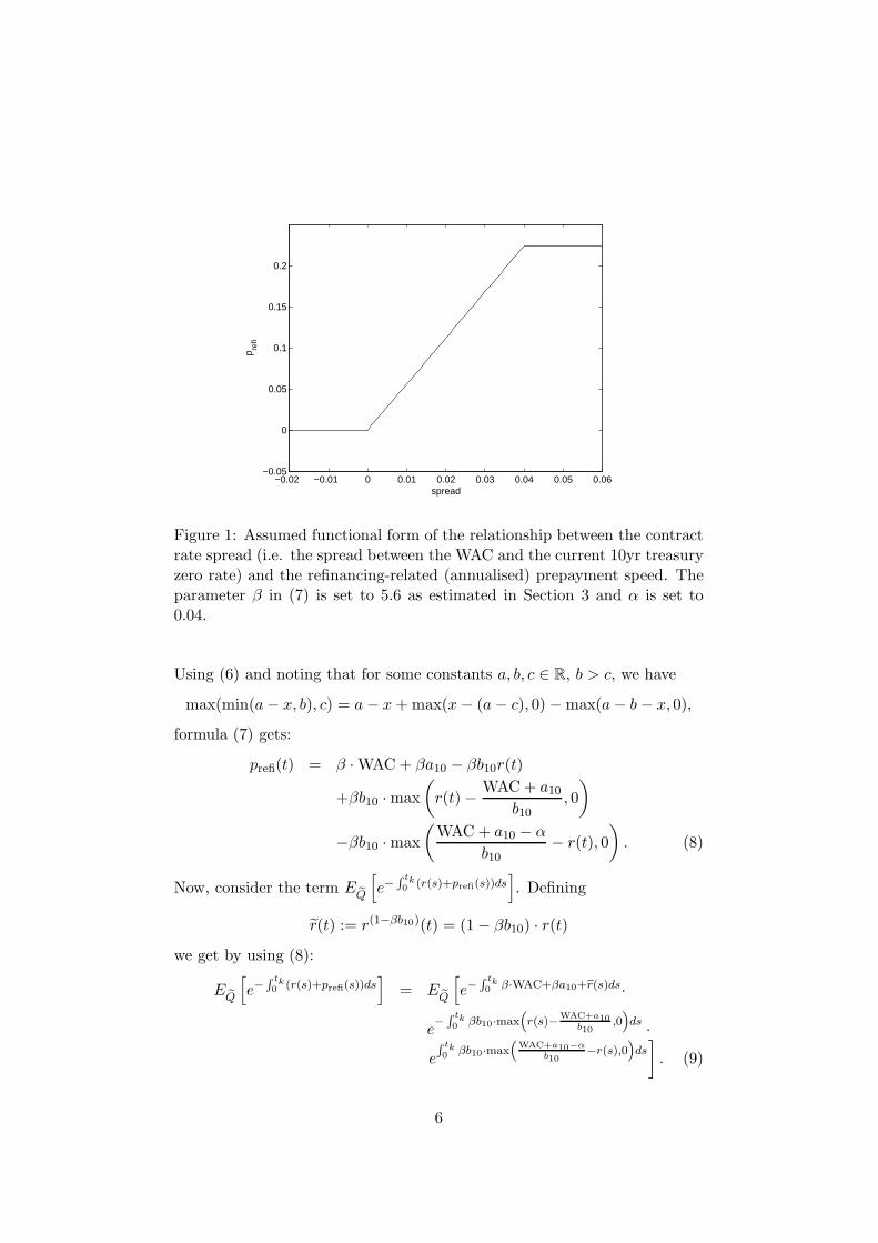
prefi(t) = β · max(min(WAC − R10(t), α), 0), (7)

for some constant α > 0, which results in a spread-refinancing prepaymentrelationship as shown in Figure 1. This functional form offers two majoradvantages compared to a purely linear functional form:

• The S-like relationship between the spread and the refinancing-drivenprepayment, which has been confirmed empirically by, e.g., Levin andDaras (1998), is accounted for.

• Refinancing-driven prepayment can never become negative.

5

−0.02 −0.01 0 0.01 0.02 0.03 0.04 0.05 0.06−0.05

0

0.05

0.1

0.15

0.2

spread

p refi

Figure 1: Assumed functional form of the relationship between the contractrate spread (i.e. the spread between the WAC and the current 10yr treasuryzero rate) and the refinancing-related (annualised) prepayment speed. Theparameter β in (7) is set to 5.6 as estimated in Section 3 and α is set to0.04.

Using (6) and noting that for some constants a, b, c ∈ R, b > c, we have

max(min(a − x, b), c) = a − x + max(x − (a − c), 0) − max(a − b − x, 0),

formula (7) gets:

prefi(t) = β · WAC + βa10 − βb10r(t)

+βb10 · max

(r(t) − WAC + a10

b10, 0

)

−βb10 · max

(WAC + a10 − α

b10− r(t), 0

). (8)

Now, consider the term E eQ

[e−

R tk0 (r(s)+prefi(s))ds

]. Defining

r(t) := r(1−βb10)(t) = (1 − βb10) · r(t)we get by using (8):

E eQ

[e−

R tk0 (r(s)+prefi(s))ds

]= E eQ

[e−

R tk0 β·WAC+βa10+er(s)ds·

e−

R tk0 βb10·max

“r(s)−

WAC+a10b10

,0”ds ·

eR tk0 βb10·max

“WAC+a10−α

b10−r(s),0

”ds]

. (9)

6

Theorem 2.2. Within the model setting as previously introduced and defin-ing

C(tk) := e−tk ·(β·WAC+βa10)

the expression

P refi(0, tk) := E eQ

[e−

R tk0 (r(s)+prefi(s))ds

]

can be reasonably approximated in the following way:

P refi(0, tk) ≈ C(tk) · P (0, tk) − C(tk) · βb10 · Cap(r, 0, tk , rCap,∆t)

+C(tk) · βb10 · Floor(r, 0, tk, rF loor,∆t), (10)

where, according to Lemma 2.1,

P (0, tk) := P (1−βb10)(0, tk)

rCap :=WAC + a10

b10

rF loor :=WAC + a10 − α

b10

Cap(r, 0, T, rX ,∆t) :=

T/∆t∑

k=1

∆t ·[q + 1 + uk

ck− uk

ck· χ2(2ckrX , 2q + 6, 2uk)

−q + 1

ck· χ2(2ckrx, 2q + 4, 2uk) − rX + rX · χ2(2ckrX , 2q + 2, 2uk)

]

Floor(r, 0, T, rX ,∆t) :=

T/∆t∑

k=1

∆t ·[rX · χ2(2ckrX , 2q + 2, 2uk)

−uk

ck· χ2(2ckrX , 2q + 6, 2uk) − q + 1

ck· χ2(2ckrX , 2q + 4, 2uk)

]

ck :=2ar

σ2r · (1 − e−ar ·k·∆t)

uk := ck · r(0) · e−ar ·k·∆t

q :=2θr

σ2r

− 1

and χ2(·; a, b) denotes the cdf of the non-central Chi-square distribution withdegrees of freedom parameter a and non-centrality parameter b.

Proof. See Appendix.

Note that the notation ”Cap” has not been chosen without motive. If oneequates the linear interest rate at time t for the period from t to t+∆t withthe short rate r(t), the expression

max

(r(k · ∆t) − (WAC + a10)

b10, 0

)· ∆t

7

in (9) is simply the payoff of a standard caplet from k · ∆t to (k + 1) · ∆twith cap rate rCap := (WAC + a10)/b10. A similar consideration applies

for the notation ”Floor”. Note also that the accuracy of the approximationin Theorem 2.2 depends, of course, on the parameter values and on theWAC of the security. In general, the approximation should be better forMBS around the current-coupon level than for deep discounts (low-couponsecurities, traded below par) or very high premiums (high-coupon securities,traded above par). We typically have ∆tk = 1/12 (i.e. 1 month) for allk = 1, ...,K. Hence, ∆t = 1/12 is a natural choice for the interval length ofthe discretisation in (10).

2.2 The baseline prepayment

We model the baseline or turnover component of prepayment within a two-factor Gaussian process framework where both factors follow Vasicek pro-cesses. The second factor is fit to the GDP growth in the US, accountingfor the dependence between general economic conditions and turnover pre-payment. Of course, any other observable factor, e.g. a suitable house priceindex, could be used instead of or in addition to the GDP growth factor.While our empirical results have turned out to be satisfactory with the GDPgrowth as second factor in the baseline prepayment model (see also Sections3 and 4), house prices have been used for example by Kariya et al. (2002),Sharp et al. (2006) or Downing et al. (2005). Our baseline prepaymentprocesses are given by their Q-dynamics

dp0(t) = (θp + bpww(t) − app0(t))dt + σpdWp(t), (11)

dw(t) = (θw − aww(t))dt + σwdWw(t),

where Wp, Ww are independent Q-Wiener processes (independent of the pre-

viously defined Wr) and ai := ai + λiσ2i , i = p,w, for the two prepayment-

risk-adjustment parameters λp, λw.In order to be able to calculate (1) we have to evaluate the expression

P d(t, T ) := E eQ[e−R T

t(er(s)+p0(s))ds]

= E eQ[e−R T

ter(s)ds] · E eQ[e−

R T

tp0(s)ds]

=: P (t, T ) · P base(t, T ),

where r(t) := r(1−βb10)(t), P (t, T ) := P (1−βb10)(t, T ). The letter d in thesuperscript of P d(t, T ) is used in analogy to the reduced-form credit riskliterature.

Theorem 2.3. In the model set-up as previously introduced it holds that

P base(t, T ) = eAd(t,T )−Cd(t,T )p0(t)−Dd(t,T )w(t)

8

with

Cd(t, T ) =1

ap

(1 − e−ap(T−t)

),

Dd(t, T ) =bpw

ap

(1 − e−aw(T−t)

aw+

e−aw(T−t) − e−ap(T−t)

aw − ap

),

Ad(t, T ) =

∫ T

t

1

2

(σ2

pCd(l, T )2 + σ2

wDd(l, T )2)

−θpCd(l, T ) − θwDd(l, T )dl.

Proof. See Appendix.

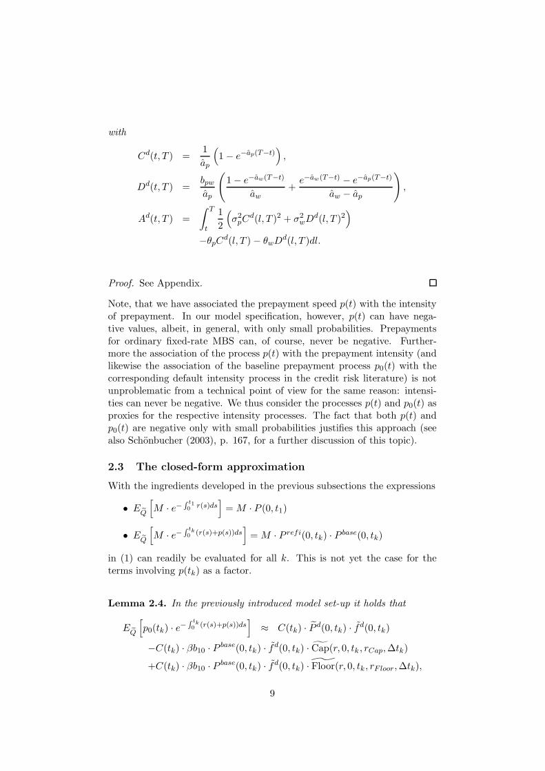
Note, that we have associated the prepayment speed p(t) with the intensityof prepayment. In our model specification, however, p(t) can have nega-tive values, albeit, in general, with only small probabilities. Prepaymentsfor ordinary fixed-rate MBS can, of course, never be negative. Further-more the association of the process p(t) with the prepayment intensity (andlikewise the association of the baseline prepayment process p0(t) with thecorresponding default intensity process in the credit risk literature) is notunproblematic from a technical point of view for the same reason: intensi-ties can never be negative. We thus consider the processes p(t) and p0(t) asproxies for the respective intensity processes. The fact that both p(t) andp0(t) are negative only with small probabilities justifies this approach (seealso Schonbucher (2003), p. 167, for a further discussion of this topic).

2.3 The closed-form approximation

With the ingredients developed in the previous subsections the expressions

• E eQ

[M · e−

R t10

r(s)ds]

= M · P (0, t1)

• E eQ

[M · e−

R tk0 (r(s)+p(s))ds

]= M · P refi(0, tk) · P base(0, tk)

in (1) can readily be evaluated for all k. This is not yet the case for theterms involving p(tk) as a factor.

Lemma 2.4. In the previously introduced model set-up it holds that

E eQ

[p0(tk) · e−

R tk0 (r(s)+p(s))ds

]≈ C(tk) · P d(0, tk) · fd(0, tk)

−C(tk) · βb10 · P base(0, tk) · fd(0, tk) · Cap(r, 0, tk , rCap,∆tk)

+C(tk) · βb10 · P base(0, tk) · fd(0, tk) · Floor(r, 0, tk , rF loor,∆tk),

9

where fd(0, tk) is the ”baseline spread forward rate”, i.e.

fd(0, tk) = − ∂

∂tkln P base(0, tk).

Proof. As a first step, recall the well-known result (see, e.g., Schmid (2004),p. 243) saying that

E eQ

[e−

R T

0r(l)dlr(T )|F0

]= −E eQ

[e−

R T

0r(l)dl|F0

]· ∂

∂Tln P (0, T ). (12)

Now, if we use use the independence between (r(t), prefi(t)) and p0(t), apply(12) to

E eQ

[p0(tk) · e−

R tk0 (r(s)+p(s))ds

]= E eQ

[e−

R tk0 (r(s)+prefi(s))ds

]·

E eQ

[p0(tk) · e−

R tk0 p0(s)ds

],

the lemma follows dircectly if we recall (10).

This leaves us with the term E eQ

[prefi(tk) · e−

R tk0 (r(s)+p(s))ds

].

Lemma 2.5. Within the previously introduced model set-up it holds that:

E eQ

[prefi(tk) · e−

R tk0 (r(s)+p(s))ds

]= −P base(0, tk) · P refi(0, tk)

· ∂

∂tkln

[P refi(0, tk)

P (0, tk)

]. (13)

Proof. If we define the tk-forward measure Qtk in the usual way via itsRadon-Nikodym derivative L(T ) with respect to Q by

L(t) =dQtk

dQ

∣∣∣∣Ft =P (t, tk)

P (0, tk) · eR tk0 r(s)ds

for t ∈ [0, tk] and use (12) we obtain:

E eQ

[prefi(tk) · e−

R tk0 (r(s)+p(s))ds

]= E eQ

[prefi(tk) · e−

R tk0 (r(s)+prefi(s))ds

]·

P base(0, tk)

= P (0, tk) · EQtk

[prefi(tk) · e−

R tk0 prefi(s)ds

]· P base(0, tk)

= −P (0, tk) · EQtk

[e−

R tk0 prefi(s)ds

]·

∂

∂tkln EQtk

[e−

R tk0 prefi(s)ds

]· P base(0, tk)

= −P refi(0, tk) · ∂

∂tkln

[P refi(0, tk)

P (0, tk)

]· P base(0, tk)

10

Note that by using Theorem 2.3 and the approximation given in Theorem2.2, it is straightforward to evaluate the terms in (13).

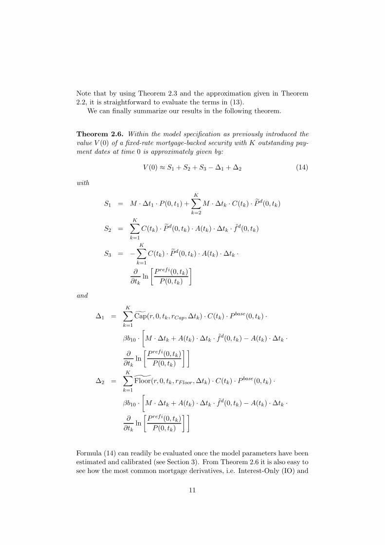
We can finally summarize our results in the following theorem.

Theorem 2.6. Within the model specification as previously introduced thevalue V (0) of a fixed-rate mortgage-backed security with K outstanding pay-ment dates at time 0 is approximately given by:

V (0) ≈ S1 + S2 + S3 − ∆1 + ∆2 (14)

with

S1 = M · ∆t1 · P (0, t1) +

K∑

k=2

M · ∆tk · C(tk) · P d(0, tk)

S2 =

K∑

k=1

C(tk) · P d(0, tk) · A(tk) · ∆tk · fd(0, tk)

S3 = −K∑

k=1

C(tk) · P d(0, tk) · A(tk) · ∆tk ·

∂

∂tkln

[P refi(0, tk)

P (0, tk)

]

and

∆1 =

K∑

k=1

Cap(r, 0, tk, rCap,∆tk) · C(tk) · P base(0, tk) ·

βb10 ·[M · ∆tk + A(tk) · ∆tk · fd(0, tk) − A(tk) · ∆tk ·

∂

∂tkln

[P refi(0, tk)

P (0, tk)

] ]

∆2 =K∑

k=1

Floor(r, 0, tk, rF loor,∆tk) · C(tk) · P base(0, tk) ·

βb10 ·[M · ∆tk + A(tk) · ∆tk · fd(0, tk) − A(tk) · ∆tk ·

∂

∂tkln

[P refi(0, tk)

P (0, tk)

] ]

Formula (14) can readily be evaluated once the model parameters have beenestimated and calibrated (see Section 3). From Theorem 2.6 it is also easy tosee how the most common mortgage derivatives, i.e. Interest-Only (IO) and

11

Principal-Only (PO) securities, can be priced within our modelling frame-work. If we split up the mortgage payment M into the interest payment M I

and regular principal repayment MP , so that M=M I + MP , and denote

SI1 := M I · ∆t1 · P (0, t1) +

K∑

k=2

M I · ∆tk · C(tk) · P d(0, tk),

∆I1 :=

K∑

k=1

Cap(r, 0, tk, rCap,∆tk) · C(tk) · P base(0, tk) · βb10 · M I · ∆tk

∆I2 :=

K∑

k=1

Floor(r, 0, tk, rF loor,∆tk) · C(tk) · P base(0, tk) · βb10 · M I · ∆tk

SP1 := S1 − SI

1

∆P1 := ∆1 − ∆I

1

∆P2 := ∆2 − ∆I

2,

we obtain the following two corollaries, which conclude this section.

Corollary 2.7. The value VIO(0) of an Interest-Only security with K out-standing payment dates at time 0 is given by:

VIO(0) = SI1 − ∆I

1 + ∆I2

Corollary 2.8. The value VPO(0) of a Principal-Only security with K out-standing payment dates at time 0 is given by:

VPO(0) = SP1 + S2 + S3 − ∆P

1 + ∆P2

3 Parameter estimation and model calibration

The available data for this study consists of US treasury strip par ratesand monthly historic prepayment data for large issues of 30yr fixed-ratemortgage-backed securities of the GNMA I and GNMA II programs. Inaddition to this we have monthly historic prices of generic GNMA 30yrpass-through MBS for a wide range of different coupons as traded on a to-be-announced (TBA) basis. All data were obtained from Bloomberg.

Weekly US treasury strip zero rates, obtained from the par rates bystandard bootstrapping, from 1993 to 2005 are used for the estimation ofthe parameters of the CIR interest-rate model. We estimate the parame-ters with a state-space approach which integrates time-series information ofdifferent maturities, similar to the approach described in Geyer and Pichler(1999). Estimation of the unobservable state variables (i.e. the short-rate) isdone with an approximative Kalman filter where the transition densities are

12

supposed to be normal. For the maximisation of the log-likelihood we usea combined Downhill Simplex/Simulated Annealing algorithm as describedin Press et al. (1992), which we also use for all following maximisation andoptimisation steps.

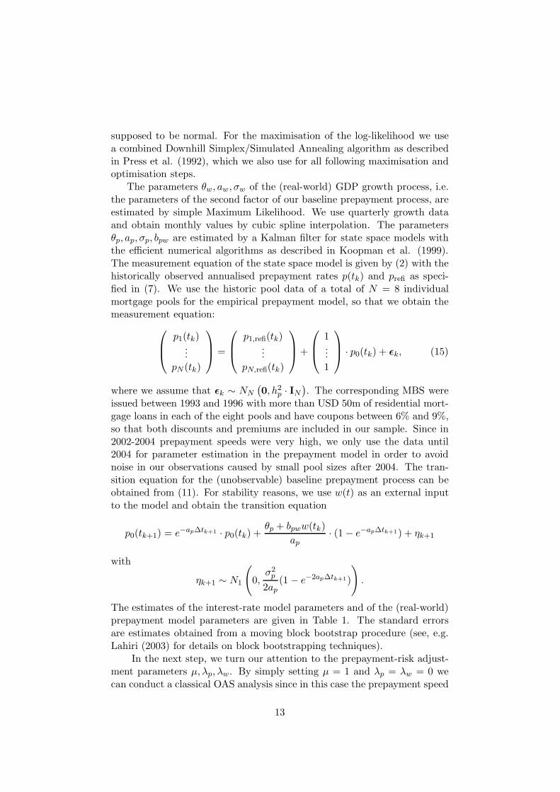
The parameters θw, aw, σw of the (real-world) GDP growth process, i.e.the parameters of the second factor of our baseline prepayment process, areestimated by simple Maximum Likelihood. We use quarterly growth dataand obtain monthly values by cubic spline interpolation. The parametersθp, ap, σp, bpw are estimated by a Kalman filter for state space models withthe efficient numerical algorithms as described in Koopman et al. (1999).The measurement equation of the state space model is given by (2) with thehistorically observed annualised prepayment rates p(tk) and prefi as speci-fied in (7). We use the historic pool data of a total of N = 8 individualmortgage pools for the empirical prepayment model, so that we obtain themeasurement equation:

p1(tk)...

pN (tk)

=

p1,refi(tk)...

pN,refi(tk)

+

1...1

· p0(tk) + ǫk, (15)

where we assume that ǫk ∼ NN

(0, h2

p · IN

). The corresponding MBS were

issued between 1993 and 1996 with more than USD 50m of residential mort-gage loans in each of the eight pools and have coupons between 6% and 9%,so that both discounts and premiums are included in our sample. Since in2002-2004 prepayment speeds were very high, we only use the data until2004 for parameter estimation in the prepayment model in order to avoidnoise in our observations caused by small pool sizes after 2004. The tran-sition equation for the (unobservable) baseline prepayment process can beobtained from (11). For stability reasons, we use w(t) as an external inputto the model and obtain the transition equation

p0(tk+1) = e−ap∆tk+1 · p0(tk) +θp + bpww(tk)

ap· (1 − e−ap∆tk+1) + ηk+1

with

ηk+1 ∼ N1

(0,

σ2p

2ap(1 − e−2ap∆tk+1)

).

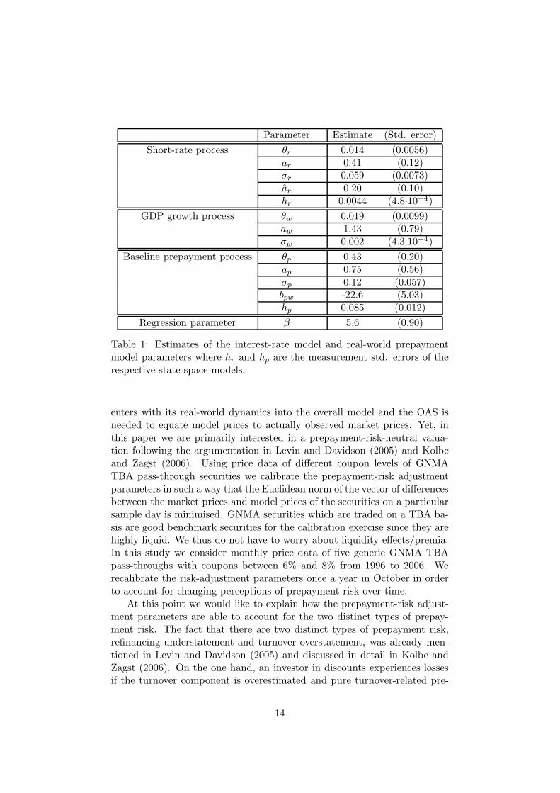
The estimates of the interest-rate model parameters and of the (real-world)prepayment model parameters are given in Table 1. The standard errorsare estimates obtained from a moving block bootstrap procedure (see, e.g.Lahiri (2003) for details on block bootstrapping techniques).

In the next step, we turn our attention to the prepayment-risk adjust-ment parameters µ, λp, λw. By simply setting µ = 1 and λp = λw = 0 wecan conduct a classical OAS analysis since in this case the prepayment speed

13

Parameter Estimate (Std. error)

Short-rate process θr 0.014 (0.0056)ar 0.41 (0.12)σr 0.059 (0.0073)ar 0.20 (0.10)hr 0.0044 (4.8·10−4)

GDP growth process θw 0.019 (0.0099)aw 1.43 (0.79)σw 0.002 (4.3·10−4)

Baseline prepayment process θp 0.43 (0.20)ap 0.75 (0.56)σp 0.12 (0.057)bpw -22.6 (5.03)hp 0.085 (0.012)

Regression parameter β 5.6 (0.90)

Table 1: Estimates of the interest-rate model and real-world prepaymentmodel parameters where hr and hp are the measurement std. errors of therespective state space models.

enters with its real-world dynamics into the overall model and the OAS isneeded to equate model prices to actually observed market prices. Yet, inthis paper we are primarily interested in a prepayment-risk-neutral valua-tion following the argumentation in Levin and Davidson (2005) and Kolbeand Zagst (2006). Using price data of different coupon levels of GNMATBA pass-through securities we calibrate the prepayment-risk adjustmentparameters in such a way that the Euclidean norm of the vector of differencesbetween the market prices and model prices of the securities on a particularsample day is minimised. GNMA securities which are traded on a TBA ba-sis are good benchmark securities for the calibration exercise since they arehighly liquid. We thus do not have to worry about liquidity effects/premia.In this study we consider monthly price data of five generic GNMA TBApass-throughs with coupons between 6% and 8% from 1996 to 2006. Werecalibrate the risk-adjustment parameters once a year in October in orderto account for changing perceptions of prepayment risk over time.

At this point we would like to explain how the prepayment-risk adjust-ment parameters are able to account for the two distinct types of prepay-ment risk. The fact that there are two distinct types of prepayment risk,refinancing understatement and turnover overstatement, was already men-tioned in Levin and Davidson (2005) and discussed in detail in Kolbe andZagst (2006). On the one hand, an investor in discounts experiences lossesif the turnover component is overestimated and pure turnover-related pre-

14

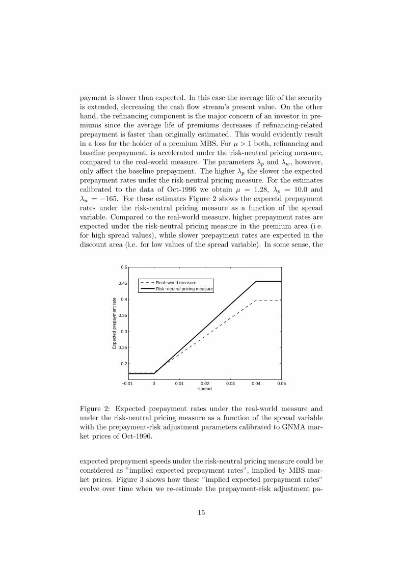
payment is slower than expected. In this case the average life of the securityis extended, decreasing the cash flow stream’s present value. On the otherhand, the refinancing component is the major concern of an investor in pre-miums since the average life of premiums decreases if refinancing-relatedprepayment is faster than originally estimated. This would evidently resultin a loss for the holder of a premium MBS. For µ > 1 both, refinancing andbaseline prepayment, is accelerated under the risk-neutral pricing measure,compared to the real-world measure. The parameters λp and λw, however,only affect the baseline prepayment. The higher λp the slower the expectedprepayment rates under the risk-neutral pricing measure. For the estimatescalibrated to the data of Oct-1996 we obtain µ = 1.28, λp = 10.0 andλw = −165. For these estimates Figure 2 shows the expecetd prepaymentrates under the risk-neutral pricing measure as a function of the spreadvariable. Compared to the real-world measure, higher prepayment rates areexpected under the risk-neutral pricing measure in the premium area (i.e.for high spread values), while slower prepayment rates are expected in thediscount area (i.e. for low values of the spread variable). In some sense, the

−0.01 0 0.01 0.02 0.03 0.04 0.05

0.2

0.25

0.3

0.35

0.4

0.45

0.5

spread

Exp

ecte

d pr

epay

men

t rat

e

Real−world measureRisk−neutral pricing measure

Figure 2: Expected prepayment rates under the real-world measure andunder the risk-neutral pricing measure as a function of the spread variablewith the prepayment-risk adjustment parameters calibrated to GNMA mar-ket prices of Oct-1996.

expected prepayment speeds under the risk-neutral pricing measure could beconsidered as ”implied expected prepayment rates”, implied by MBS mar-ket prices. Figure 3 shows how these ”implied expected prepayment rates”evolve over time when we re-estimate the prepayment-risk adjustment pa-

15

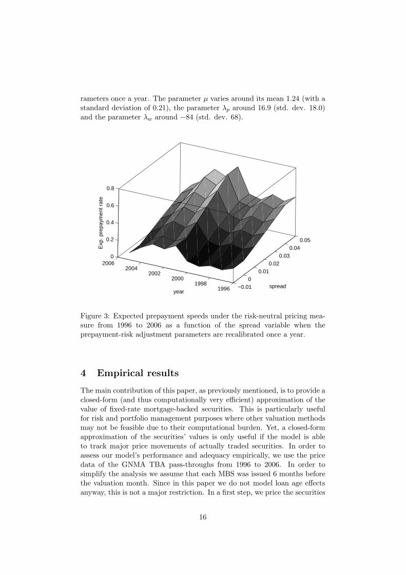
rameters once a year. The parameter µ varies around its mean 1.24 (with astandard deviation of 0.21), the parameter λp around 16.9 (std. dev. 18.0)and the parameter λw around −84 (std. dev. 68).

−0.010

0.010.02

0.030.04

0.05

19961998

20002002

20042006

0

0.2

0.4

0.6

0.8

spreadyear

Exp

. pre

paym

ent r

ate

Figure 3: Expected prepayment speeds under the risk-neutral pricing mea-sure from 1996 to 2006 as a function of the spread variable when theprepayment-risk adjustment parameters are recalibrated once a year.

4 Empirical results

The main contribution of this paper, as previously mentioned, is to provide aclosed-form (and thus computationally very efficient) approximation of thevalue of fixed-rate mortgage-backed securities. This is particularly usefulfor risk and portfolio management purposes where other valuation methodsmay not be feasible due to their computational burden. Yet, a closed-formapproximation of the securities’ values is only useful if the model is ableto track major price movements of actually traded securities. In order toassess our model’s performance and adequacy empirically, we use the pricedata of the GNMA TBA pass-throughs from 1996 to 2006. In order tosimplify the analysis we assume that each MBS was issued 6 months beforethe valuation month. Since in this paper we do not model loan age effectsanyway, this is not a major restriction. In a first step, we price the securities

16

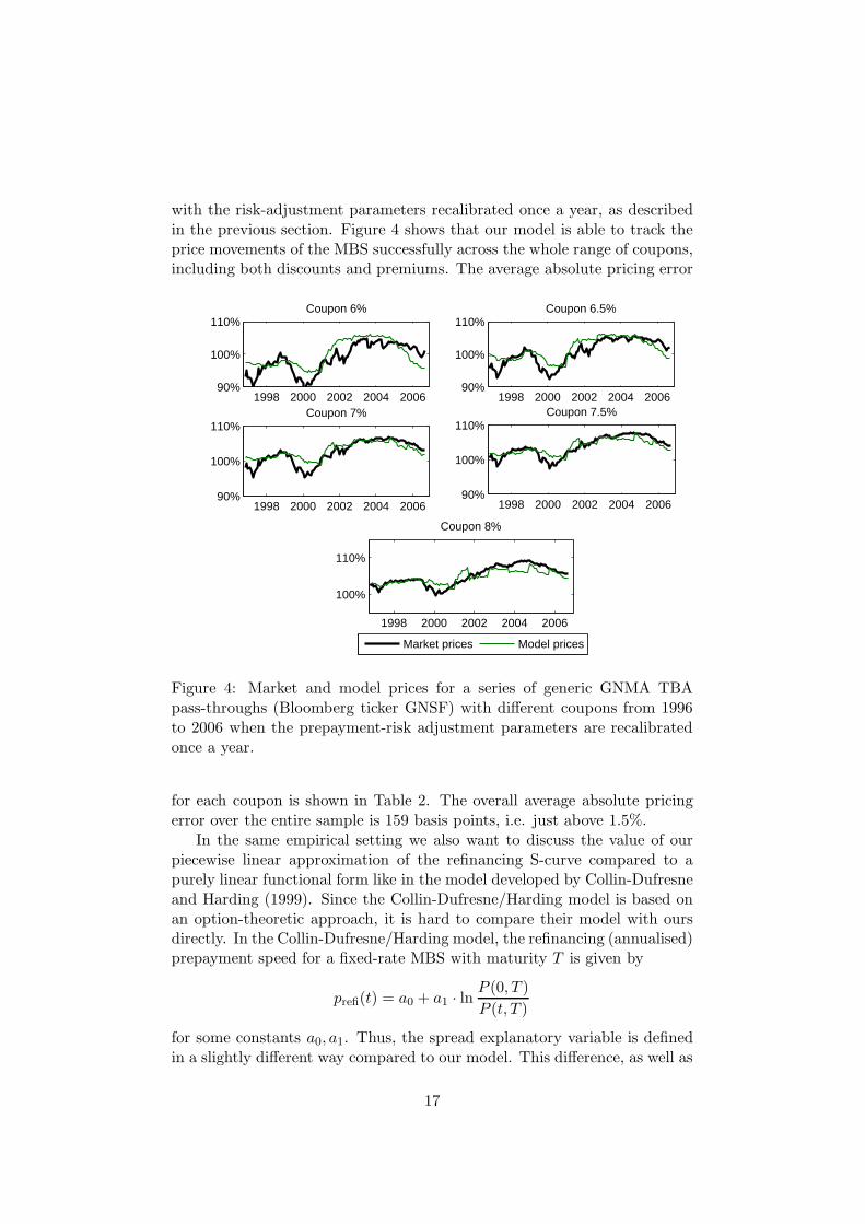
with the risk-adjustment parameters recalibrated once a year, as describedin the previous section. Figure 4 shows that our model is able to track theprice movements of the MBS successfully across the whole range of coupons,including both discounts and premiums. The average absolute pricing error

1998 2000 2002 2004 200690%

100%

110%Coupon 6%

1998 2000 2002 2004 200690%

100%

110%Coupon 6.5%

1998 2000 2002 2004 200690%

100%

110%Coupon 7%

1998 2000 2002 2004 200690%

100%

110%Coupon 7.5%

1998 2000 2002 2004 2006

100%

110%

Coupon 8%

Market prices Model prices

Figure 4: Market and model prices for a series of generic GNMA TBApass-throughs (Bloomberg ticker GNSF) with different coupons from 1996to 2006 when the prepayment-risk adjustment parameters are recalibratedonce a year.

for each coupon is shown in Table 2. The overall average absolute pricingerror over the entire sample is 159 basis points, i.e. just above 1.5%.

In the same empirical setting we also want to discuss the value of ourpiecewise linear approximation of the refinancing S-curve compared to apurely linear functional form like in the model developed by Collin-Dufresneand Harding (1999). Since the Collin-Dufresne/Harding model is based onan option-theoretic approach, it is hard to compare their model with oursdirectly. In the Collin-Dufresne/Harding model, the refinancing (annualised)prepayment speed for a fixed-rate MBS with maturity T is given by

prefi(t) = a0 + a1 · lnP (0, T )

P (t, T )

for some constants a0, a1. Thus, the spread explanatory variable is definedin a slightly different way compared to our model. This difference, as well as

17

the fact that Collin-Dufresne and Harding (1999) use a Vasicek process forthe short-rate, can be considered as minor differences between the models.Apart from the restriction to one stochastic factor, the major restriction inthe Collin-Dufresne/Harding model is the purely linear form for the approx-imation of the refinancing S-curve. Within our model framework, we wantto test empirically whether the piecewise linear approximation presented inthis paper does add explanatory power to the pricing model. For this pur-pose we re-estimate our model with a purely linear functional form. I.e.,instead of (7) we set:

prefi(t) = β · (WAC − R10(t)).

Note that there is no need for an intercept here since we still incorporatethe baseline prepayment process p0(t). This, of course, makes the formulamuch easier since we do not have to deal with the rather complex formulasof Theorem 2.2. We also re-calibrate the risk-adjustment parameters once ayear and price the five different coupon securities with this model from 1996to 2006. The results as shown in Table 2 indicate that the piecewise linearapproximation yields indeed better results than the purely linear functionalform, almost across the whole coupon range. The overall average absolutepricing error is 266 basis points in the model with a purely linear functionalform, compared to 159 basis points in our full model.

Coupon Average abs. pricing error Average abs. pricing error(full model, in basis points) (linear model, in basis points)

6% 266 380

6.5% 187 142

7% 141 165

7.5% 116 230

8% 121 402

Table 2: Average absolute pricing errors of our full model and of themodel with a purely linear spread/prepayment speed relation for a seriesof generic GNMA TBA pass-throughs (Bloomberg ticker GNSF) with dif-ferent coupons from 1996 to 2006 when the prepayment-risk adjustmentparameters are recalibrated once a year.

In a second step we calibrate the prepayment-risk adjustment parame-ters only once to the data of Oct-1996 and leave them unchanged for the restof the time period considered in this study. In this out-of sample experiment(w.r.t. the prepayment-risk adjustment parameters), our model is still ableto explain the observed market prices with a satisfactory accuracy. Theaverage absolute pricing error for each coupon is shown in Table 3 together

18

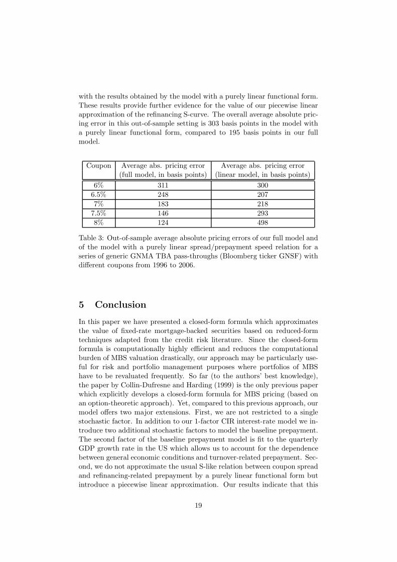
with the results obtained by the model with a purely linear functional form.These results provide further evidence for the value of our piecewise linearapproximation of the refinancing S-curve. The overall average absolute pric-ing error in this out-of-sample setting is 303 basis points in the model witha purely linear functional form, compared to 195 basis points in our fullmodel.

Coupon Average abs. pricing error Average abs. pricing error(full model, in basis points) (linear model, in basis points)

6% 311 300

6.5% 248 207

7% 183 218

7.5% 146 293

8% 124 498

Table 3: Out-of-sample average absolute pricing errors of our full model andof the model with a purely linear spread/prepayment speed relation for aseries of generic GNMA TBA pass-throughs (Bloomberg ticker GNSF) withdifferent coupons from 1996 to 2006.

5 Conclusion

In this paper we have presented a closed-form formula which approximatesthe value of fixed-rate mortgage-backed securities based on reduced-formtechniques adapted from the credit risk literature. Since the closed-formformula is computationally highly efficient and reduces the computationalburden of MBS valuation drastically, our approach may be particularly use-ful for risk and portfolio management purposes where portfolios of MBShave to be revaluated frequently. So far (to the authors’ best knowledge),the paper by Collin-Dufresne and Harding (1999) is the only previous paperwhich explicitly develops a closed-form formula for MBS pricing (based onan option-theoretic approach). Yet, compared to this previous approach, ourmodel offers two major extensions. First, we are not restricted to a singlestochastic factor. In addition to our 1-factor CIR interest-rate model we in-troduce two additional stochastic factors to model the baseline prepayment.The second factor of the baseline prepayment model is fit to the quarterlyGDP growth rate in the US which allows us to account for the dependencebetween general economic conditions and turnover-related prepayment. Sec-ond, we do not approximate the usual S-like relation between coupon spreadand refinancing-related prepayment by a purely linear functional form butintroduce a piecewise linear approximation. Our results indicate that this

19

contributes to a significant improvement of the model performance.Applied to historic price data of 30yr GNMA pass-throughs traded on a

TBA basis, our model proves to be able to explain major market price move-ments succesfully for a wide range of coupons. The overall average absolutepricing error of 159 basis points in our sample (with a yearly recalibrationof prepayment-risk adjustment parameters) indicates a highly satisfactoryaccuracy of our model for risk and portfolio management purposes.

Our model also provides a further motivation for a thorough empiricalstudy about which and how many factors are needed to adequately pricemortgage-backed securities. In many previous pricing models this discus-sion was restricted due to the model specification and the computationalburden associated with additional factors. While this is beyond the scope ofthis paper, our model may provide a basis for further empirical contributionsin this field.

A Proof of Lemma 2.1:

For c = 1 we have the well-known formulas for zero-coupon bond prices inthe CIR model. For c ≥ 0 in general, we get the dynamics of rc(t) under Qby a simple application of the Ito-formula and obtain:

rc(t) = (θcr − arr

c(t))dt + σcr

√rc(t)dWr(t)

with

θcr = c · θr,

σcr =

√c · σr

and the statement follows directly from, e.g., Zagst (2002), p.126/127. For

− a2r

2σ2r≤ c < 0, however, the result is less straightforward. We therefore

explicitly give the detailed proof in the following.From the Feynman-Kac representation of the Cauchy-Problem (see, e.g.

Zagst (2002), [2.6]) we know that P c(t, T ) must satisfy:

P ct + (θr − arr)P

cr +

1

2· σ2

r · rP crr = c · r · P c (16)

with boundary condition P c(T, T ) = 1. Since

P cr = −Bc · P c,

P ct = P c · (Ac

t − r · Bct ),

P crr = (Bc)2 · P c,

it follows from (16) that

Act(t, T )−θrB

c(t, T )−r · (c− 1

2·σ2

r · (Bc(t, T ))2 +Bct (t, T )− ar ·Bc(t, T )) = 0

20

with Ac(T, T ) = Bc(T, T ) = 0. This leads to the Riccati-style equations

c − 1

2· σ2

r · (Bc(t, T ))2 + Bct (t, T ) − arB

c(t, T ) = 0

with Bc(T, T ) = 0 andAc

t(t, T ) = θrBc(t, T )

with Ac(T, T ) = 0. By simple calculations it can be verified that

Bc(t, T ) = c · 1 − e−γc(T−t)

κ1 − κ2e−γc(T−t),

Ac(t, T ) =2θr

σ2r

log

[γceκ2·(T−t)

κ1 − κ2 · e−γc·(T−t)

]

with γc :=√

a2r + 2σ2

rc, κ1 := ar

2 + γc

2 and κ2 := ar

2 − γc

2 solve the Riccati

equations for c ≥ − a2r

2σ2r.

B Proof of Theorem 2.2:

After factoring out C(tk) in (9) we apply the approximation

ex+y+z ≈ 1 + x + y + z ≈ ex + y + z.

For our purposes, this is a sufficiently good approximation since the quanti-ties corresponding to x, y, z in (9) are small. If we approximate the integralsby sums, we obtain:

E eQ

[e−

R tk0 (r(s)+prefi(s))ds

]≈ C(tk) · P (0, tk)

−βb10 · C(tk) · ∆t ·⌈

tk∆t

⌉∑

k=1

E eQ

[max

(r(k · ∆t) − WAC + a10

b10, 0

)]

+βb10 · C(tk) · ∆t ·⌈

tk∆t

⌉∑

k=1

E eQ

[max

(WAC + a10 − α

b10− r(k · ∆t), 0

)]

= C(tk) · P (0, tk)

−βb10 · C(tk) · ∆t ·⌈

tk∆t

⌉∑

k=1

∫ ∞

rCap

(r(k · ∆t) − rCap) f(r(k · ∆t))dr(k · ∆t)

+βb10 · C(tk) · ∆t ·⌈

tk∆t

⌉∑

k=1

∫ rF loor

0(rF loor − r(k · ∆t)) f(r(k · ∆t))dr(k · ∆t),

(17)

21

where f(·) denotes the pdf of the short rate. Since we work with a CIRmodel in this paper, we know from Cox et al. (1985) that the distribution of2 · ck · r(k ·∆t) is the non-central χ2-distribution with parameters 2q +2 and2uk, with ck, uk and q as previously defined. From the recurrence relation(see Johnson et al. (1995), p. 442)

λ · χ2(x;µ + 4, λ) = (λ − µ) · χ2(x;µ + 2, λ)

+(x + µ) · χ2(x;µ, λ) − x · χ2(x;µ − 2, λ)

(18)

(for µ > 2) and from the relation (see Johnson et al. (1995), p. 443)

∂χ2(x;µ, λ)

∂x= f(x;µ, λ) =

1

2(χ2(x;µ − 2, λ) − χ2(x;µ, λ)) (19)

it follows with some easy calculations that∫ b

0xf(x;µ, λ)dx = µ · χ2(b;µ + 2, λ) + λ · χ2(b;µ + 4, λ). (20)

Applying (20) to the first integral in (17), we obtain:∫ ∞

rCap

(r(k · ∆t) − rCap) f(r(k · ∆t))dr(k · ∆t) =1

2ck

[E eQ[2ckr(k · ∆t)] −

−(2q + 2) · χ2(2ckrCap; 2q + 4, 2uk) − 2uk · χ2(2ckrCap; 2q + 6, 2uk)

]

−rCap · (1 − χ2(2ckrCap; 2q + 2, 2uk)).

Similarly,∫ rF loor

0(rF loor − r(k · ∆t)) f(r(k · ∆t))dr(k · ∆t) =

rF loor · χ2(2ckrF loor; 2q + 2, 2uk) − 1

2ck

[(2q + 2)

·χ2(2ckrF loor; 2q + 4, 2uk) + 2uk · χ2(2ckrF loor; 2q + 6, 2uk)

].

Noting thatE eQ[2ckr(k · ∆t)] = 2q + 2 + 2uk,

formula (10) follows directly after rearranging of terms.

C Proof of Theorem 2.3:

From the Feynman-Kac representation of the Cauchy-Problem (see, e.g.Zagst (2002), [2.6]) we know that P base(t, T ) must satisfy:

P baset + (θw − aww)P base

w + (θp + bpw · w − app0)Pbasep0

+1

2· (σ2

p · P basep0p0

+ σ2w · P base

ww ) = p0 · P base

22

Calculating the derivatives of P base it follows that

Adt (t, T ) − p0(1 − apC

d(t, T ) + Cdt (t, T ))

−w(Ddt (t, T ) − awDd(t, T ) + bpwCd(t, T ))

+12 · (σ2

pCd(t, T )2 + σ2

wDd(t, T )2) − θpCd(t, T ) − θwDd(t, T ) = 0.

Thus, we obtain the system of linear differential equations

1 − apCd(t, T ) + Cd

t (t, T ) = 0

bpwCd(t, T ) − awDd(t, T ) + Ddt (t, T ) = 0

Adt (t, T ) +

1

2· (σ2

pCd(s, T )2 + σ2

wDd(s, T )2)

−θpCd(s, T ) − θwDd(s, T ) = 0

with Ad(T, T ) = 0, Cd(T, T ) = Dd(T, T ) = 0. With some easy calculationsit is straightforward to verify that the formulas as stated in Theorem 2.3 arethe solutions of the linear differential equations above.

References

Bielecki, T. and M. Rutkowski (2002). Credit Risk: Modeling, Valuationand Hedging. Berlin: Springer.

Collin-Dufresne, P. and J. Harding (1999). A Closed Form Formula forValuing Mortgages. Journal of Real Estate Finance and Economics 19-2, 133–146.

Cox, J., J. Ingersoll, and S. Ross (1985). A Theory of the Term Structureof Interest Rates. Econometrica 53-2, 385–408.

Downing, C., R. Stanton, and N. Wallace (2005). An Empirical Test of aTwo-Factor Mortgage Valuation Model: How Much Do House PricesMatter? Real Estate Economics 33, 681–710.

Geyer, A. and S. Pichler (1999). A state-space approach to estimate andtest multifactor Cox-Ingersoll-Ross models of the term structure. Jour-nal of Financial Research 22-1, 107–130.

Goncharov, Y. (2005). An Intensity-Based Approach to Valuation ofMortgage Contracts and Computation of the Endogenous MortgageRate. International Journal of Theoretical and Applied Finance 9-6,889–914.

Johnson, L., S. Kotz, and N. Balakrishnan (1995). Continuous UnivariateDistributions, Vol. 2, 2nd edition. New York: John Wiley & Sons.

Kalotay, A., D. Yang, and F. Fabozzi (2004). An Option-Theoretic Pre-payment Model for Mortgages and Mortgage-Backed Securities. Inter-national Journal of Theoretical and Applied Finance 7, 949–978.

23

Kariya, T., F. Ushiyama, and S. Pliska (2002). A 3-factor Valuation Modelfor Mortgage-Backed Securities. Working Paper .

Kau, J., D. Keenan, and A. Smurov (2004). Reduced-Form MortgageValuation. Working Paper .

Kolbe, A. and R. Zagst (2006). A Hybrid-Form Model for the Valuationof Mortgage-Backed Securities. Working Paper .

Koopman, S., N. Shephard, and J. Doornik (1999). Statistical algorithmsfor models in state space using Ssfpack 2.2. Econometrics Journal 2,113–166.

Kupiec, P. and A. Kah (1999). On the Origin and Interpretation of OAS.The Journal of Fixed Income 9-3, 82–92.

Lahiri, S. (2003). Resampling Methods for Dependent Data. New York:Springer.

Levin, A. and D. Daras (1998). Non-Traded Factors in MBS Portfo-lio Management, Advances in the Valuation and Management ofMortgage-Backed Securities (F. Fabozzi, ed.). New Hope: Frank J.Fabozzi Associates.

Levin, A. and A. Davidson (2005). Prepayment Risk- and Option-Adjusted Valuation of MBS - Opportunities for Arbitrage. The Journalof Portfolio Management 31-4.

Press, W., S. Teukolsky, W. Vetterling, and B. Flamery (1992). NumericalRecipes in C, The Art of Scientific Computing (2nd edition). Cam-bridge: Cambridge University Press.

Schmid, B. (2004). Credit Risk Pricing Models: Theory and Practice (2ndedition). Berlin: Springer Finance.

Schonbucher, P. (2003). Credit derivatives pricing models. Chichester:John Wiley & Sons.

Schwartz, E. and W. Torous (1989). Prepayment and the Valuation ofMortgage-Backed Securities. The Journal of Finance 44, 375–392.

Sharp, N., D. Newton, and P. Duck (2006). An Improved Fixed-RateMortgage Valuation Methodology With Interacting Prepayment andDefault Options. Journal of Real Estate Finance and Economics,forthcoming .

Stanton, R. (1995). Rational Prepayment and the Valuation of Mortgage-Backed Securities. Review of Financial Studies 8, 677–708.

Zagst, R. (2002). Interest Rate Management. Berlin: Springer Finance.

24