the sensitivity of repeat and near repeat analysis to
TRANSCRIPT
The Sensitivity of Repeat and Near Repeat Analysis to Geocoding Algorithms
Cory P. Haberman, PhD
School of Criminal Justice
University of Cincinnati
David Hatten
Department of Criminal Justice
John Jay College of Criminal Justice, City University of New York
Jeremy G. Carter, PhD
Paul H. O’Neill School of Public and Environmental Affairs
Indiana University – Purdue University Indianapolis
Eric L. Piza, PhD
Department of Criminal Justice
John Jay College of Criminal Justice, City University of New York
Abstract
Purpose: To determine if repeat and near repeat analysis is sensitive to the geocoding algorithm
used for the underlying crime incident data.
Methods: The Indianapolis Metropolitan Police Department provided 2016 crime incident data
for five crime types: (1) shootings, (2) robberies, (3) residential burglaries, (4) theft of
automobiles, and (5) theft from automobiles. The incident data were geocoded using a dual
ranges algorithm and a composite algorithm. First, descriptive analysis of the distances between
the two point patterns were conducted. Second, repeat and near repeat analysis was performed.
Third, the resulting repeat and near repeat patterns were compared across geocoding algorithms.
Results: The underlying point patterns and repeat and near repeat analyses were similar across
geocoding algorithms.
Conclusions: While detailing geocoding processes increases transparency and future researchers
can conduct sensitivity results to ensure their findings are robust, dual ranges geocoding
algorithms are likely adequate for repeat and near repeat analysis.
Key Words
Repeat Victimization, Near Repeat Victimization, Geocoding, Spatiotemporal Analysis
Citation
Haberman, C. P., Hatten, D., Carter, J.G., and Piza, E.L. (2020). The sensitivity of repeat and
near repeat analysis to geocoding algorithms. Journal of Criminal Justice, DOI:
10.1016/j.jcrimjus.2020.101721.
HEADER: Sensitivity of Repeat and Near Repeat Analysis to Geocoding Algorithms
1
INTRODUCTION
Scholarly interest in spatiotemporal analyses of event data is surging in the social sciences.
In the context of criminology, this interest is driven in large part by evidence related to crime
concentration at place (Weisburd, 2015), place-based intersections of public health, crime, and
disorder (Ratcliffe 2015, White & Weisburd, 2018), effectiveness of place-based crime prevention
and hot spots policing at reducing crime (Braga, Papachristos & Hureau, 2019), and the emergence
of predictive policing (Caplan et al., 2019; Mohler et al., 2015). In this vein, repeat and near-repeat
(R/NR) spatiotemporal modeling of crime has emerged as an important research area, particularly
given its implications for certain crime prevention tactics and predictive policing models (e.g. see
Mohler et al., 2011). R/NR analyses seek to identify contagion or diffusion patterns of crime events
in space and time. Such analyses are reliant upon the positional accuracy of spatial data and
appropriateness of the geocoding method employed. Findings from R/NR analyses are in turn used
to inform police and crime prevention strategies - thus appropriate geocoding procedures are
salient to deploy effective interventions. From an academic perspective, study replication and
pursuit of knowledge relies on carefully articulated methodologies. To this end, we examine
whether the results of R/NR analyses for various crime types are sensitive to the geocoding
algorithm used.
REPEAT & NEAR REPEAT CRIME PATTERNS
To understand the variability of geocoding procedures employed in R/NR analyses, we
conducted a comprehensive review of the R/NR literature in criminology and criminal justice. This
review yielded 82 unique studies. Several notable themes were evident and pertinent to the current
study. First and foremost, only ~21 percent of studies (n = 17) reported the geocoding algorithm
HEADER: Sensitivity of Repeat and Near Repeat Analysis to Geocoding Algorithms
2
used.1 This is both surprising and concerning for reasons articulated in the discussion below.
Second, R/NR studies are frequently published in high-ranking criminology and criminal justice
journals that often place an increased emphasis on methodological rigor and clarity. For example,
41 percent (n = 33) of the studies identified in our review were published in Journal of Quantitative
Criminology; Justice Quarterly; Journal of Research in Crime and Delinquency; Journal of
Experimental Criminology; British Journal of Criminology; Crime & Delinquency, Criminal
Justice and Behavior; Police Quarterly; and European Journal of Criminology. Third, 68 percent
of the studies identified had been published since 2012, while 42 percent have been published
since 2017. This dramatic upward trend is likely to continue as the interest in, and application of,
R/NR analyses receive further scholarly attention to help explain a range of crime and place
phenomena. Lastly, approximately half of the studies leverage data from the United States, while
the other half represent notable international variability across study locations such as United
Kingdom, Australia, China, Africa, Austria, Iraq, Netherlands, Turkey, Spain, Germany, Sweden,
and New Zealand. This geographic dispersion illustrates the wide-spread interest in R/NR crime
patterns, but also the varying geographic, social, and cultural contexts within which these analyses
are executed – further demanding the need for refined geocoding processes and reporting.
Nonetheless, R/NR patterns have been identified for multiple crime types, such as:
Residential burglary (Bernasco, 2008; Bowers & Johnson, 2004, 2005; Chainey et al.,
2018; Gerstner, 2018; Groff & Taniguchi, 2019a, 2019b; Johnson, 2008, 2013; Johnson et
al., 2007),
Aggravated assault (Kennedy et al., 2016; Zhang et al., 2015),
1 A table including results of this review is available as online supplemental material.
HEADER: Sensitivity of Repeat and Near Repeat Analysis to Geocoding Algorithms
3
Motor vehicle theft (Block & Fujita, 2013; de Melo et al., 2018; Lockwood, 2012; Piza &
Carter, 2018; Youstin et al., 2011),
Theft from vehicles (Emeno & Bennell, 2018; Johnson et al., 2009),
Arson (Grubb & Nobles, 2016; Turchan et al., 2018),
Shootings (Loeffler & Flaxman, 2018; Mazeika & Uriarte, 2018; Ratcliffe & Rengert,
2008; Renda & Zhang; Sturup et al., 2018; Wells et al., 2012; Wells & Wu, 2011; Youstin
et al., 2011),
Robbery (Garnier et al., 2018; Glasner & Leitner, 2017; Grubesic & Mack, 2008;
Haberman & Ratcliffe, 2012),
Terrorism (Behlendorf et al., 2012; Braithwaite & Johnson, 2012, 2015; Johnson &
Braithwaite, 2009; LaFree et al., 2012; Townsley, Johnson, & Ratcliffe, 2008),
Maritime piracy (Marchione & Johnson, 2013; Townsley & Oliveria, 2015), and
Economic crimes such as counterfeiting and fraud (Powell, Grubb & Nobles, 2018; Wilson
& Fulmer, 2014).
There are two dominant theoretical explanations as to why R/NR crime patterns exist. The
risk heterogeneity perspective – also referred to as the “flag hypothesis” – asserts that different
geographies have different propensities for crime (Bowers & Johnson, 2005; Pease, 1998; Sparks,
1981). Such places exhibit time-stable environmental characteristics that are conducive to crime
and signal to offenders a perceived suitability for crime. Geographic risk heterogeneity is akin to
explanations of crime concentration at place (Weisburd, 2015), which are most highly
concentrated at micro localized scales (O’Brien, 2019). Alternatively, the state-dependence
perspective – also referred to as the “boost hypothesis” - asserts crime has a contagion affect
wherein previous offending influences future risk of similar crime events (Bowers & Johnson,
HEADER: Sensitivity of Repeat and Near Repeat Analysis to Geocoding Algorithms
4
2004; Nobles et al., 2016; Ornstein & Hammond, 2017; Ratcliffe & Rengert, 2008). The boost
hypothesis has been evidenced in offender foraging studies of crime (Bernasco, 2008; Johnson,
Summers, & Pease, 2009), indicating that offenders develop local, crime-specific knowledge
during the course of an original offense that in turn influences the likelihood of future offending
in that same location. Moreover, recent research suggests offenders develop time-specific
knowledge of their offending environments (van Sleeuwen, Ruiter, & Menting, 2018) and share
this learned knowledge among their co-offending networks, thereby increasing the risk that
previous victimization will repeat (Lantz & Ruback, 2017).
Finally, R/NR analysis has import for crime prevention and policing strategies. Though hot
spots policing has demonstrated crime prevention benefits (Braga et al., 2019), R/NR crime events
occur within and outside of places identified by police as stable criminogenic micro-places (Gorr
& Lee, 2015; McLaughlin et al., 2007; Mohler et al., 2011). Analogous to near-repeat crime events,
Santos and Santos (2015a, 2015b) observed police patrol and enforcement could result in
significant crime reductions for burglary and thefts from vehicle in micro-time hot spots, or crime
“flare ups” which mirror patterns of near-repeat events. In short, micro-time hot spots are clusters
or chains of near-repeat events. Moreover, a recent experiment directed 20-minute patrols to
micro-time property crime hot spots and observed significant crime reductions out to 30 days; with
greatest treatment effects observed in the immediate 15 days following identification of treatment
locations (Santos & Santos, 2020).
Likewise, R/NR patterns underpin other crime prevention tactics, such as cocoon watch
(Farrell & Pease, 2017) or citizen notification (Groff & Taniguchi, 2019b), albeit the prevention
potential requires careful consideration (Groff & Taniguchi, 2019a). Studies in Europe found
significant crime reductions focused on R/NR crime events occurring in multi-family housing
HEADER: Sensitivity of Repeat and Near Repeat Analysis to Geocoding Algorithms
5
complexes and neighborhoods (Anderson, Chenery, & Pease, 1995; Chenery, Holt, & Pease 1997;
Johnson et al., 2017). In the United States, Groff and Taniguchi (2019b) conducted a randomized
control trial in Redlands, California and Baltimore County, Maryland focused on R/NR residential
burglaries. Police employed uniformed volunteers to notify residents in near repeat areas of
increased risk, resulting in a slight reduction in burglary events. Similarly, interventions leveraging
citizen notification pamphlets in areas where an originating event occurred have demonstrated
significant crime reductions (Thompson, Townsley, & Pease, 2008; Stokes & Clare, 2019).
R/NR analysis also underpins some predictive policing models (Johnson et al., 2007, 2009;
Johnson & Bowers, 2004; Mohler et al., 2011). As the recent National Academies of Sciences,
Engineering, and Medicine (2018, p. 131-132) report on proactive policing noted:
“Other predictive analytical approaches may be useful, especially the near-repeat
techniques that use short-term event patterns to forecast probabilities of future
events… These approaches could be more effective at predicting short-term crime
hot spots than traditional crime mapping approaches, though the methods to assess
predictive accuracy have not yet been generally agreed upon and different
approaches often produce different types of crime forecast from different data
sources - further confounding comparisons”.
Nonetheless, patrols focused on short-term predicted locations have been effective (Mohler et al.,
2011).
However, such crime prevention benefits of R/NR events are contingent upon proper
geocoding and police capacity (Goff & Taniguchi, 2019b). From an analytic perspective, recent
research suggests near-repeat events vary by geography (Chainey et al., 2018) and thus expected
crime prevention benefits are dependent upon the frequency of such events in a given place and
positional accuracy of such events (Groff & Taniguchi, 2019a). Haberman and Ratcliffe (2012)
also note the limited ability of police to translate the empirical reality of R/NR crime events into
tangible prevention benefits. They note police agencies must have a robust crime analysis unit that
operates in short-term frequencies as well as nimble decision-making processes and tactical
HEADER: Sensitivity of Repeat and Near Repeat Analysis to Geocoding Algorithms
6
resources to respond within the minimal near-repeat temporal window. Overall, R/NR patterns can
inform policing and crime prevention strategies, but precise identification of R/NR patterns is
paramount.
GEOCODING IN THE CONTEXT OF REPEAT AND NEAR-REPEAT CRIMES
The Technical Details of Geocoding
Geocoding is the process of converting addresses to XY-coordinates (Chainey & Ratcliffe,
2005). In general, geocoding algorithms take (1) a list of addresses and attempt to locate them
within (2) references database(s) (Zandbergen, 2009). The optional plural of database(s) in the
previous sentence is one important component that distinguishes geocoding algorithms.
Ideally, analysts would have reference data capturing all possible addresses and the
addresses’ corresponding XY-coordinates (Zandbergen, 2008). The geocoding algorithm would
then simply match crime incidents’ addresses to the master address list to obtain a set of
corresponding XY-coordinates. Master address reference databases might include address points
or parcels. While hardware, software, and data collection limitations have meant that digital master
address lists have been rarely available and used to geocode crime, they have recently become
more common (Zandbergen, 2009).2 Further, researchers have argued these reference data more
accurately capture locations in the physical world (e.g. see Mazeika & Summerton, 2017).
Nonetheless, fully geocoding crime incident addresses with a master address list is
typically infeasible due to how crimes occur and incidents’ addresses are recorded (Bichler &
Balchak, 2007; Brimicombe et al., 2007). First, crimes that occur outdoors do not technically occur
at a single, physical address linking to a structure. Second, some crimes occur at a “fuzzy address”
where the incident starts at one location and occurs at another (e.g. when a robber follows a victim
2 In some jurisdictions, parcels may not represent a true master address list as one parcel can contain many addresses
that are not official recorded in a parcel dataset (Zandbergen, 2008).
HEADER: Sensitivity of Repeat and Near Repeat Analysis to Geocoding Algorithms
7
from a bar and commits the act a few blocks away). Third, and related to the previous two points,
there are many complexities with how officers record addresses when taking crime reports. One
issue is that officers often estimate crime incident addresses. For example, a victim might point to
a general area where an assault took place, and the officer will simply select or even interpolate a
nearby address (or intersection). Therefore, crime incidents’ addresses often do not link to a
physical structure or are a rough approximation.
As such, crime incidents are typically geocoded using the “dual ranges” geocoding
algorithm based on a street centerline reference dataset (Hart & Zandbergen, 2013; Zandbergen,
2008). In a street centerline GIS layer, a single line digitally represents all lanes of a street segment,
hence the term “centerline”. Underlying attribute data describe each street segment’s
characteristics, such as the street name, prefix, suffix, address range, and so on. Using topology,
typically odd address ranges are represented on one side the street segment and even addresses on
the other side just as they are in the real world.3 The dual ranges geocoding algorithm then
geocodes a crime incident to the correct street segment based on the name attributes and the correct
side of the street segment based on the numerical address values and topological principles. The
numerical ranges for a street segment, however, present another complexity. The location of each
address on a street segment is interpolated. One can imagine each segment as a number line with
each side of the street segment having a “from address” or the starting value of the address range
and a “to address” or the ending value of the address range. All address values for one side of the
street segment are assumed to be equally spaced along the street segment. When geocoding is
conducted, the respective location for the corresponding address value is selected and the
corresponding XY-coordinates for the location are used for that crime incident. Finally, two more
3 While extremely rare, we recognize it is not always true that odd and even numbered addresses are on opposite sides
of the street.
HEADER: Sensitivity of Repeat and Near Repeat Analysis to Geocoding Algorithms
8
complexities are introduced into the dual ranges geocoding algorithm. Because the street
centerlines are a generalization and there is often physical space between the centerline and
structures on that street (i.e., lanes, sidewalks, and maybe yards) an “offset” is applied. The offset
is a constant spatial distance in which each geocoded address is moved away from the centerline
roughly perpendicularly in order to place points closer to where the actual structure for the address
might be on the street. Likewise, it is rare for structures to sit right on a street centerline endpoint
due to lanes, sidewalks, and yards on cross streets, so an “endset” is applied. This is a
predetermined spatial distance or proportion of the total street segment’s length measured from the
intersection where addresses are excluded from geocoding to again provide a more realistic
portrayal of where an address might be located in physical space. Thus, it is easy to see how
geocoding using the dual ranges algorithm is an estimate of an address’ actual location of in
physical space.
Finally, an alternative approach is to use a “composite” geocoding algorithm (e.g. see
Brimicombe et al., 2007). Composite geocoding uses multiple geocoding algorithms to assign XY-
coordinates to incident addresses. Composite algorithms use a hierarchy system to geocode
addresses with multiple algorithms. An obvious combination would be to first attempt to geocode
to a master address list (e.g. parcel file), and then move to a dual ranges algorithm. Hypothetically,
the algorithm could continue attempting to match addresses to higher-level geographies, such as
zip code centroids and ultimately city centroids. While matching to these higher-level spatial units
would increase one’s hit-rate (rate at which addresses are successfully matched), it would provide
relatively inaccurate XY-coordinates in relation to where a crime incident actually occurred.
Once geocoding is complete, a geocoding algorithm can be evaluated across at least three
criteria: (1) positional accuracy, (2) completeness, and (3) repeatability (Hart & Zandbergen, 2013;
HEADER: Sensitivity of Repeat and Near Repeat Analysis to Geocoding Algorithms
9
Zandbergen, 2009). Positional accuracy is the extent to which a geocoded location matches its
actual location. Completeness is the extent to which the geocoding algorithm can identify XY-
coordinates for the address list (i.e. match or hit-rate). Repeatability is the extent to which the
geocoding results can be replicated across variations on the algorithm parameters.
Most crime and place methodology sections only assess and report completeness (i.e. hit-
rate) (Mazeika & Summerton, 2017). In fact, most studies simply state the geocoding hit-rate met
or exceeded Ratcliffe’s (2004) recommended 85% “acceptable minimum hit-rate” (but see
Andresen et al., 2020; Briz-Redón et al., 2019). While typically not discussed, the positional
accuracy of crime data geocoding is just as important as completeness (Bichler & Balchak, 2007;
Mazeika & Summerton, 2017; Zandbergen, 2008, 2009). Low geocoding hit-rates would call into
the question the use of a dataset, but an analyst could also easily achieve a 100% hit-rate by
sacrificing positional accuracy. For example, one could simply geocode crime data to city,
neighborhood, or police district centroids or allow for less stringent geocoding parameters
(Mazeika & Summerton, 2017) to obtain a 100% hit-rate, but the process would result in geocoded
incidents too positionally inaccurate to appropriately describe the spatial crime patterns.
To date, the limited research available suggests that geocoding quality impacts spatial
crime analysis. First, positional accuracy can be impacted by a number of factors, such as the
quality of crime incidents’ address input or the underlying reference data (Bichler & Balchak,
2007; Hart & Zandbergen, 2012; Mazeika & Summerton, 2017). Second, the results of some
analytical techniques commonly used in crime analysis are sensitive to geocoding results. For
example, kernel density estimation appears to be impacted by geocoding quality. Brimicombe and
colleagues (2007) suggested unmatched crime incidents might have kernel density intensities that
differ from matched incidents (i.e., missing hot spots). Alternatively, Harada and Shimada (2006)
HEADER: Sensitivity of Repeat and Near Repeat Analysis to Geocoding Algorithms
10
demonstrated some differences in two kernel density surfaces produced from the same crime
incident dataset geocoded at two levels of precision. In addition, geocoding methods can impact
distance calculations. Zandbergen and Hart (2009) showed how the positional inaccuracies from
geocoding sex offenders’ residences and restricted locations using a dual ranges algorithm (and
assuming parcels represent accurate locations) produced errors where sex offenders would be both
incorrectly determined in compliance and in violation of residency restriction laws. It follows that
crime and place studies should provide geocoding details in their methodology sections as the
method employed may influence the studies’ results.
Geocoding Crime Incidents for Near Repeat Analysis
Recall, only ~21% studies (n=17) identified in a review of R/NR literature identified the
geocoding method. Geocoding methods using street centerline and parcel centroid reference
datasets were most commonly reported, followed by an even mixture of grid cell, street segment,
and block centroid techniques. The lack of discussion concerning geocoding method and spatial
data preparation is especially troubling for R/NR studies given distances among crime incidents is
a key parameter in R/NR analysis. Specifically, the assignment of spatial locations of crime
incidents are dependent upon geocoding method and this process may skew the premise of a “near”
repeat event. For example, if a vehicle is stolen in the parking lot of a large mall, this crime event
could be assigned to the parcel centroid (parcel geocoding) or the nearest major road segment (dual
ranges geocoding), which are potentially quite distant from each other. This example highlights
two issues that would influence the validity of the results of the R/NR analyses. First, the difference
in the assignment of spatial location across geocoding methods causes concern for repeatability of
the study. Second, in terms of positional accuracy, the assigned location could potentially be
several thousand feet from where the crime occurred, drastically misrepresenting the spatial
HEADER: Sensitivity of Repeat and Near Repeat Analysis to Geocoding Algorithms
11
location of the event. Moreover, while this may be less of a cause for concern for one or two thefts,
when there are several thousand being considered for any given year, the problem is magnified.
This is especially true when the events are proximal to residential areas where the theft event may
be closer to capturing residential attributes as opposed to commercial characteristics as would be
the case of where the actual crime occurred. Both issues influence the extent to which R/NR
analyses can generate reliable results to appropriately inform police strategic operations.
DATA & METHOD
Data
The present study used official crime incident data from the Indianapolis Metropolitan
Police Department (IMPD). Indianapolis is the largest city in the state of Indiana, the state capital,
and a consolidated city-county municipality. In 2016, Indianapolis had a population of 867,125
persons with a population density of 2,270 persons per square mile. The largest ethnic group in
Indianapolis is non-Hispanic White consisting of 55.9% of the total population with much smaller
proportions of non-White racial/ethnic groups (28.1% Black, 10.1% Hispanic, and 3.0% Asian).
Median household income in 2010 was $44,709 and Indianapolis had 20.1% of residents living
below the poverty line (as compared to 13.5% statewide). Additionally, 29.7% of the population
had a bachelor’s degree or higher as compared to 25.3% statewide.4 Indianapolis reported a violent
crime rate of 1,374 crimes per 100,000 residents compared to 876 per 100,000 for all cities of a
similar population in the United States (500,000 - 999,999 residents). In addition, robbery and
burglary rates in Indianapolis were similarly high for all cities of a similar population at (458 vs.
282) and (1,178 vs. 768), respectively. The reported motor vehicle theft rate was 576 vs. 525 per
100,000.5
4 All sociodemographic figures based on 2010 ACS estimates 5 As per FBI Crime in the United States, 2016. All crime rates are per 100,000 residents.
HEADER: Sensitivity of Repeat and Near Repeat Analysis to Geocoding Algorithms
12
IMPD provided 2016 crime incident data for five crime types: (1) homicides or aggravated
assaults with a firearm (hereafter shootings), (2) robberies, (3) residential burglaries, (4) theft of
automobiles, and (5) theft from automobiles. Incidents for each crime type were identified using
UCR classification codes. IMPD’s crime incident data are susceptible to all of the well-known
limitations of official crime data, such as victim and officer reporting and recoding discretion
(Wolfgang, 1963).
Analytic Plan
Two geocoding methods were compared. First, a dual ranges address locator was created
using an official street centerline file from IMPD. A dual ranges address locator effectively
represents the standard geocoding method used for research and crime analysis. An offset of 20
feet was used. An endset of 3% was used as that is the default value in ESRI’s ArcGIS which is
commonly used in practice (e.g. see Mazeika & Summerton, 2017: endnote 4). Second, a
composite address locator using both parcels and street address ranges was used. The parcel data
were procured from the IndyGIS open data portal. The street centerline file from the dual ranges
address locator was re-used. All remaining parameters were the same as during the dual ranges
geocoding process.6 The use of composite algorithms made up of separate parcel-based and dual-
range algorithms helps to maximize the geocoding hit-rate, as certain common police reporting
practices, such as recording incident addresses as street corners (e.g. “Main St. and Central Ave.”)
rather than precise addresses (e.g. “100 Main St.”) (Braga, Papachristos, & Hureau, 2010),
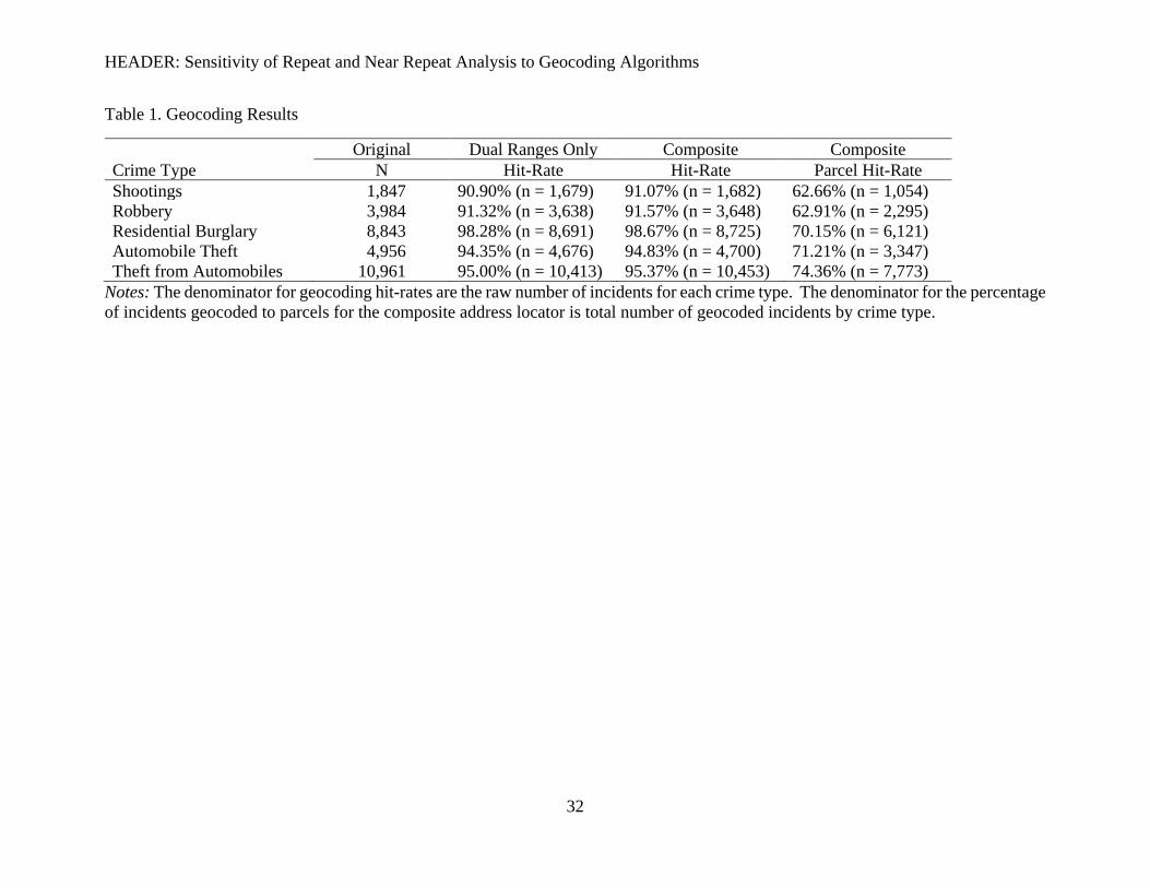
generates incident locations that cannot be matched to parcels (Piza & Carter 2018). Table 1
6 Another option is to use a proprietary geocoding service, such as the Google Geocoding API (Mazeika & Summerton,
2017). This option was not used for the following reasons. First, the proprietary nature of those options sometimes
means the exact parameters used are unknown and may not be disclosed due to market competition. Likewise, details
about the underlying reference data used in those processes may not be provided for the same reasons. Third,
proprietary geocoding services can be costly. Fourth, given the vast amount of geographic data now collected by
government agencies, there is no evidence or reason to believe that geocoding algorithms built with freely available
local data are inferior to proprietary geocoding services.
HEADER: Sensitivity of Repeat and Near Repeat Analysis to Geocoding Algorithms
13
displays the original raw incidents counts before geocoding, geocoding hit-rates for both methods,
and the percentage of all incidents matched using the composite address locator that were matched
to a parcel.7
After geocoding was completed, the first set of analyses examined the distances between
the incidents’ two sets of XY-coordinates to assess how the geocoding method impacted incidents’
locations. Distance was computed using Manhattan distance.8 Descriptive statistics for the
distances between crime incidents’ locations by geocoding type were computed. Next, because
near repeat analyses commonly use street block distances for the spatial bandwidth (discussed in
detail below) (e.g. see Haberman & Ratcliffe, 20102; Piza & Carter, 2018), the percentage and
frequency of incidents at incremental street blocks distances away from each other were examined.
If the two geocoding methods commonly locate the same incidents a street block or more from
each other, then it would suggest those incidents would often be counted in different spatial
bandwidths during R/NR analyses and knowing that detail would help understand how geocoding
methods may impact near repeat analyses. In Indianapolis, the average street block is about 434
feet (Piza & Carter, 2018), so multiples of 434 feet approximated street block distances.
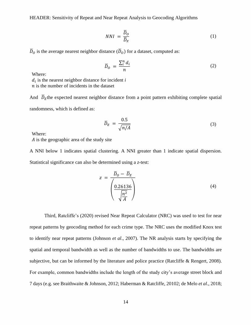
The second set of analyses explored the point-patterns generated by both geocoding
methods. A nearest neighbor index (NNI) was computed for both sets of geocoded incidents for
each crime type. The NNI is a common measure of spatial concentration, and a component of other
spatial statistics, such as nearest neighbor hierarchical clustering (Chainey & Ratcliffe, 2005, pg.
126). All nearest neighbor calculations were computed in ArcGIS 10.3, which defines the NNI as:
7 The number of incidents matched to a parcel for the composite address locator is equivalent to the number of incidents
that would have been matched using a parcel-only address locator. Thus, a hit-rate for a parcel-only address locator
could be computed using the number of incidents matched to a parcel and the original incidents counts shown in Table
1. 8 As a sensitivity check, all analyses were also computed using Euclidean distance. The results using Euclidean
distance are presented in the Online Appendix, but they were substantively similar to those reported herein using
Manhattan distance.
HEADER: Sensitivity of Repeat and Near Repeat Analysis to Geocoding Algorithms
14
𝑁𝑁𝐼 = �̅�𝑂�̅�𝐸
(1)
�̅�𝑂 is the average nearest neighbor distance (�̅�𝑂) for a dataset, computed as:
�̅�𝑂 = ∑ 𝑑𝑖𝑛𝑖
𝑛 (2)
Where:
𝑑𝑖 is the nearest neighbor distance for incident i
𝑛 is the number of incidents in the dataset
And �̅�𝐸the expected nearest neighbor distance from a point pattern exhibiting complete spatial
randomness, which is defined as:
�̅�𝐸 = 0.5
√𝑛/𝐴 (3)
Where:
𝐴 is the geographic area of the study site
A NNI below 1 indicates spatial clustering. A NNI greater than 1 indicate spatial dispersion.
Statistical significance can also be determined using a z-test:
𝑧 = �̅�𝑂 − �̅�𝐸
(
0.26136
√𝑛2
𝐴 )
(4)
Third, Ratcliffe’s (2020) revised Near Repeat Calculator (NRC) was used to test for near
repeat patterns by geocoding method for each crime type. The NRC uses the modified Knox test
to identify near repeat patterns (Johnson et al., 2007). The NR analysis starts by specifying the
spatial and temporal bandwidth as well as the number of bandwidths to use. The bandwidths are
subjective, but can be informed by the literature and police practice (Ratcliffe & Rengert, 2008).
For example, common bandwidths include the length of the study city’s average street block and
7 days (e.g. see Braithwaite & Johnson, 2012; Haberman & Ratcliffe, 20102; de Melo et al., 2018;
HEADER: Sensitivity of Repeat and Near Repeat Analysis to Geocoding Algorithms
15
Piza & Carter, 2018). The bandwidths inform the creation of a contingency table where each cell
represents a spatial-temporal distance combination extending out to some maximum number of
bandwidths. The spatial and temporal distances from each incident to every other incident in the
analysis dataset is computed and the number of point-pairs within each cell of the contingency
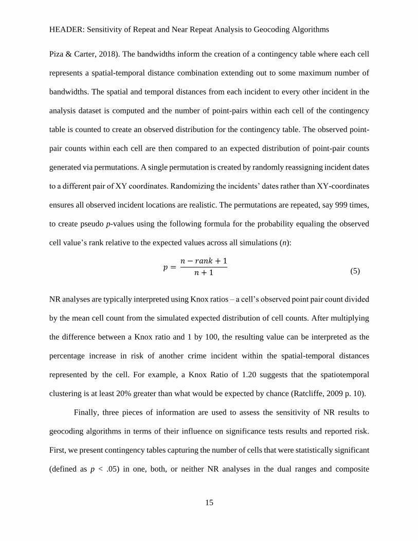
table is counted to create an observed distribution for the contingency table. The observed point-
pair counts within each cell are then compared to an expected distribution of point-pair counts
generated via permutations. A single permutation is created by randomly reassigning incident dates
to a different pair of XY coordinates. Randomizing the incidents’ dates rather than XY-coordinates
ensures all observed incident locations are realistic. The permutations are repeated, say 999 times,
to create pseudo p-values using the following formula for the probability equaling the observed
cell value’s rank relative to the expected values across all simulations (n):
𝑝 = 𝑛 − 𝑟𝑎𝑛𝑘 + 1
𝑛 + 1
(5)
NR analyses are typically interpreted using Knox ratios – a cell’s observed point pair count divided
by the mean cell count from the simulated expected distribution of cell counts. After multiplying
the difference between a Knox ratio and 1 by 100, the resulting value can be interpreted as the
percentage increase in risk of another crime incident within the spatial-temporal distances
represented by the cell. For example, a Knox Ratio of 1.20 suggests that the spatiotemporal
clustering is at least 20% greater than what would be expected by chance (Ratcliffe, 2009 p. 10).
Finally, three pieces of information are used to assess the sensitivity of NR results to
geocoding algorithms in terms of their influence on significance tests results and reported risk.
First, we present contingency tables capturing the number of cells that were statistically significant
(defined as p < .05) in one, both, or neither NR analyses in the dual ranges and composite
HEADER: Sensitivity of Repeat and Near Repeat Analysis to Geocoding Algorithms
16
geocoding algorithms. This contingency table quantifies the extent to which the choice of
geocoding method influences the significance testing component of R/NR analyses. Second, the
full extent of the NR patterns were compared across geocoding algorithms to determine if different
conclusions would be drawn from the individual analyses. The full extent of the NR pattern for
each geocoding algorithm is identified by reading the Knox Ratios in the output table from the
top-left through the bottom-right on the diagonal and noting which cells achieved statistical
significance and how the difference in spatial-temporal risk changes across the table. Generally, it
is expected that NR risk will decrease moving along the diagonal, and an analyst will describe the
extent of the NR pattern by describing the lower and upper space-time bandwidths that achieved
statistical significance (e.g. see Haberman & Ratcliffe, 2012). Third, differences in the magnitudes
of the Knox Ratios were computed by dividing the dual ranges method Knox Ratios by the
composite method Knox Ratios. A ratio value equal to 1 suggests identical risk levels were
identified for a space-time bandwidth between geocoding methods. Ratios greater than 1 suggest
the dual-range algorithms resulted in higher reported risk than the composite algorithms for a given
space-time bandwidth. A ratio value less than 1 suggests the composite algorithm resulted in higher
reported risk than the dual ranges algorithm. The ratios are converted to percentage differences in
magnitude by multiplying the difference between the ratios and 1 by 100. The degree to which
there is a lack of agreement, in terms of reported risk, has implications for whether that cell is
suitable for translation to crime prevention and police operations as it may be overly sensitive to
geocoding method.
RESULTS
Table 1 displays the geocoding results. First, for both the dual ranges and composite
algorithms and all crime types, the geocoding hit-rate was 90.90% or greater. Thus, it would be
HEADER: Sensitivity of Repeat and Near Repeat Analysis to Geocoding Algorithms
17
reasonable to use the dataset from either geocoding algorithm for spatial analysis according to
Ratcliffe’s (2004) recommended 85% hit-rate as well as more recent estimates of minimum
acceptable geocoding rates (Andresen et al., 2020; Briz-Redón et al., 2019). Second, the
differences between the dual ranges and composite algorithms’ hit-rates at less than 1% for each
crime type are relatively trivial. Third, for the composite address locator, the percentage of
incidents geocoded to a parcel was 62.66% (n = 1,054) for shootings, 62.91% (n = 2,295) for
robbery, 70.15% (n = 6,121) for residential burglary, 71.21% (n = 3,347) for auto theft, and 74.36%
(n = 7,773) for theft from motor vehicles. Therefore, a parcel only address locator would produce
inadequate hit-rates (~57 to 71%) for all crime types (see footnote 7). Overall, Table 1 suggests
that while more than a majority of incidents of each crime type would be geocoded to a parcel
using the composite address locator, the dual ranges and composite algorithms both provide
adequate data for spatial analysis (while a parcel only address locator would not).
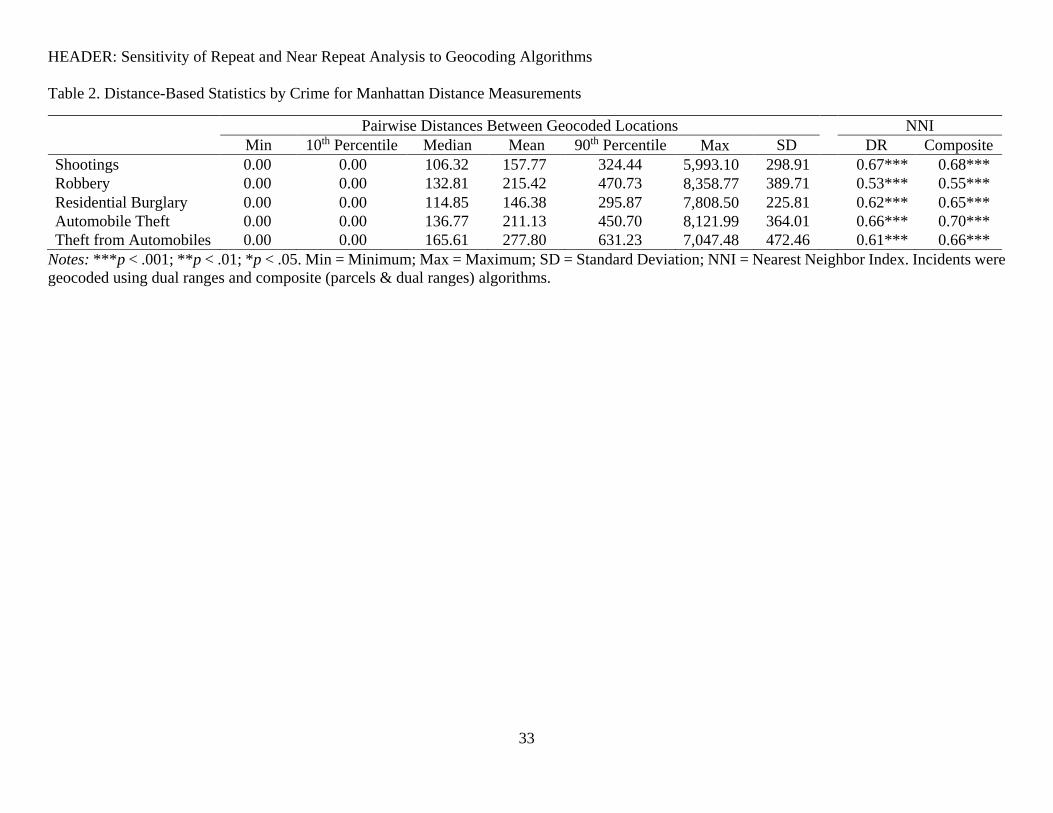
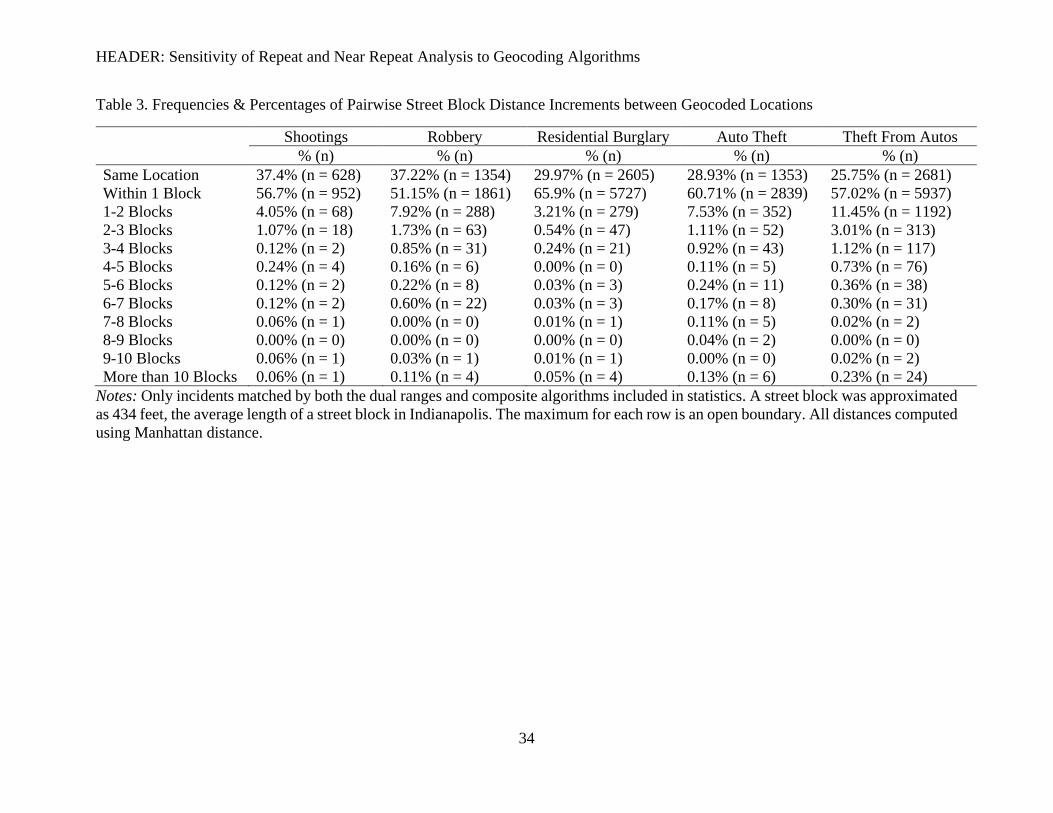
Table 2 shows descriptive statistics for the distances measured between incidents’
geocoded locations from each geocoding method. Table 3 provides frequencies of the distances
between incidents’ geocoded locations from each geocoding method using incremental street block
distances (434 feet). Table 2 shows the mean distance between geocoded incidents range from
146.38 feet (residential burglary) to roughly 277.80 feet (theft from automobiles); both distances
are less than an average city block in Indianapolis (434 feet). The relatively short distances between
the incident’s two geocoded locations is reflected in the fact that anywhere from about 25.75%
(Theft from Autos) to 37.4% (Shootings) of incidents of a given crime type were geocoded to the
same location by each algorithm (Table 3). Because the composite address locator geocoded
incidents to parcels first, another away to think about the incidents geocoded to the same location
by both methods is that they are the incidents geocoded using address ranges by both algorithms.
HEADER: Sensitivity of Repeat and Near Repeat Analysis to Geocoding Algorithms
18
Nonetheless, ~51% to 66% incidents were geocoded within 1 street block (or 434 feet) of each
other (Table 3). Finally, the NNI analysis suggested that all datasets, regardless of the address
locator, exhibited similar spatial clustering. Overall, the two methods almost always geocoded the
incidents to approximately similar locations.
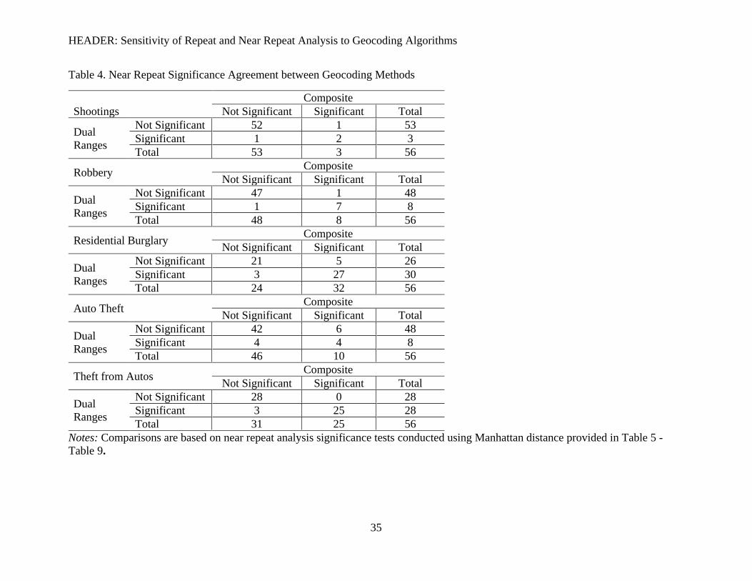
Finally, the relative similarities in the point-patterns across the two geocoding methods was
ultimately shown in the consistency of the near repeat analyses. First, Table 4 displays the simple
comparisons of how many cells achieved statistical significance (p < 0.05) between two geocoding
methods by crime type. Divergent results would occur when a cell would have been statistically
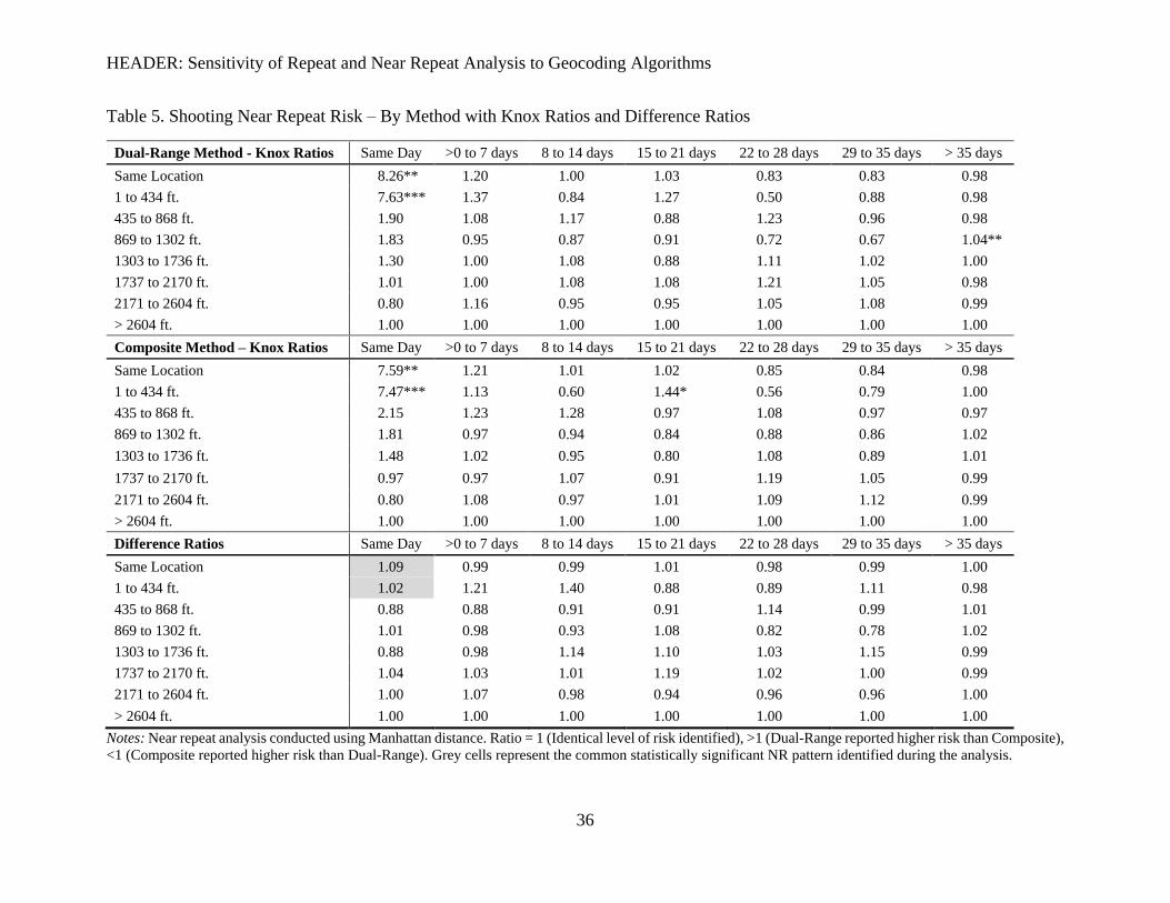
significant for a NR analysis using one geocoding method but not the other. Second, Table 5
through Table 9 show the NR results for each crime type. Each NR results table displays the Knox
Ratios produced for both geocoding algorithms in the top two panels and ratios of the Knox Ratios
in the third panel. The ratios of the Knox Ratios show relative differences in the risk levels
observed between the two geocoding methods In the bottom panel of each NR results table, grey
shading is used to show cells where the spatial-temporal bandwidths were statistically significant
(p < 0.05) for both geocoding methods, thus capturing the extent of the common NR pattern for
both geocoding algorithms. Recall the extent of the NR pattern would have implications for how
crime prevention and policing programs would be implemented using the NR results.
For the shootings, the NR results were substantively identical. Only 2 cells showed
divergent significance pattern between the dual ranges and composite geocoding methods (Table
4), but those cells that appear to be false-positives as opposed to substantive findings (i.e., errant
cells disconnected from the top-left NR pattern). Overall, there was a statistically significant risk
of a subsequent shooting on the same day, extending out about one block from the original location
regardless of whether a dual ranges or composite address locator was used. The Knox Ratios show
HEADER: Sensitivity of Repeat and Near Repeat Analysis to Geocoding Algorithms
19
roughly the same risk levels for the NR patterns identified for both geocoding methods. The two
Knox Ratios making up the statistically significant NR pattern were only about 2% or 9% larger
for the dual ranges geocoding results.
The NR robbery patterns were also substantively similar across geocoding methods. First,
only two NR result cells had divergent statistical significance patterns between geocoding methods
(Table 4). Second, again, when reading along the top-left to bottom-right diagonal, the identified
NR patterns were mostly robust to geocoding method. There was one divergence for the NR results
for the composite geocoding algorithm data identified; the NR pattern extended out to almost 3
blocks from the originator event on the same day (Table 6). Third, there was also relatively
minimal differences in the magnitudes of the Knox Ratios for the analyses using different
geocoding algorithms. For the primary NR robbery pattern, grey cells in Table 6, were about 1 to
20% different in magnitude. Overall, the substantive conclusions from NR robbery analyses were
mostly robust to geocoding methods.
For the residential burglary NR results, there were 8 cells (14%) showing different
significance patterns diverging between the two geocoding methods (Table 4). If one is basing the
extent of the NR pattern off of connecting only statistically significant cells along the top-left to
bottom-right diagonal (grey cells in the bottom panel of Table 7), a consistent NR pattern was
found extending out about two blocks and up to 21 days from an originator residential burglary
event. However, discrepancies between the geocoding methods appear in the next spatial
bandwidth (3 blocks). In the dual ranges data, the cells for 3 blocks and up to 7 days achieved
statistical significance but the cells for 3 blocks and 8 to 21 days were statistically insignificant,
whereas all four of those cells were all statistically significant in the composite geocoded data.
Additionally, the cells for 4 and 5 blocks away and extending out to 21 days from the originator
HEADER: Sensitivity of Repeat and Near Repeat Analysis to Geocoding Algorithms
20
event also mostly achieved statistical significance for both geocoding methods but 1 cell did not
(5 blocks and >0 to 7 days). The remaining cells with divergent significance patterns were more
dispersed across the space-time bandwidths and likely would not impact an analyst’s conclusions
(Table 7). Albeit it is possible that some analysts would ignore the two statistically insignificant
cells when determining the scope of their NR pattern, it is fair to say the residential burglary NR
results showed some sensitivity to geocoding method. Nonetheless, in the bottom panel of Table
7, the ratios of Knox Ratios showed only slight differences each across the two geocoding methods.
The largest difference in Knox Ratios for the cells capturing the NR pattern specifically was only
about 5%.
For auto theft, there were 10 cells with divergent statistical significance (Table 4).
Nonetheless, the NR results were consistent across geocoding methods. In short, all analyses
suggest that the most consistent risk of subsequent auto theft victimization is at the same location
for up to 7 days after an originating event (Table 8). It follows that the divergent significance
patterns in the NR results were for cells that were dispersed across the overall results table, and,
as such, are likely false positives that would not provide an analyst with any extra actionable
information about NR patterns. The bottom panel of Table 8 shows the actual Knox Ratios also
only differed in magnitude by about 1 or 2%.
Finally, the theft from autos NR results were also nearly identical across geocoding
methods. There were only 3 diverging statistical significance cells (Table 4), and the extent of the
theft from auto NR victimization pattern was consistent across all geocoding algorithms (see
bottom panel of Table 9). An increased risk of another theft from auto was found at the same
location for up to 35 days after an originator event. Additionally, there was an increased risk of
theft from auto victimization for up to 6 blocks away and within the first 7 days after an originator
HEADER: Sensitivity of Repeat and Near Repeat Analysis to Geocoding Algorithms
21
event. Nonetheless, the ratios of Knox Ratios show some variability. Most Knox Ratios were only
a few percentage points larger or smaller regardless of geocoding method, but the differences
between 4 Knox Ratios were 10% or more. Overall, the results were not sensitive enough across
geocoding algorithms to impact the design of any crime prevention or policing strategies.
DISCUSSION
This study examined if R/NR analysis results were sensitive to the geocoding algorithm
used for the underlying crime incident data. They were not. In short, while there were some
differences in significance patterns and Knox Ratios, the differences were relatively trivial and
unlikely to impact how an analyst would define the R/NR risk pattern for implementing a crime
prevention or policing strategy. In fact, residential burglary was the only crime exhibiting even
marginal sensitivity to the geocoding algorithm used, and it is still likely that analysts would have
arrived at the same R/NR patterns for operational purposes despite the slight differences.
Spatiotemporal analysis has become commonplace in criminological pursuits to better
understand crime. Unfortunately, methodological transparency has not kept pace with this surge
in analytic capacity. Specific to the R/NR literature, our literature review revealed a lack of
specificity regarding data preparation and geocoding procedures upon which replicable science
and effective interventions are developed. Fortunately, our results suggest that the conclusions
drawn from the R/NR literature likely have not been impacted by the geocoding algorithms used.
Nonetheless, it would be beneficial for the field to provide detailed descriptions of the geocoding
algorithms used for crime data used in spatial-temporal analyses given the potential for variation
in the reporting and collecting of spatial data as previously discussed. At minimum, researchers
should report (1) the geocoding algorithm used, (2) the parameters used by the algorithm, (3) the
geocoding hit-rate, and (4) any efforts to assess the positional accuracy of their geocoding process.
HEADER: Sensitivity of Repeat and Near Repeat Analysis to Geocoding Algorithms
22
This will provide transparency to readers for how the results were generated and is necessary for
informing future replication studies or potential comparisons of results across studies.
Additionally, researchers and analysts can conduct sensitivity analyses using different
geocoding algorithms to ensure their results are robust. Like many studies, external validity is one
limitation of this work, and it is unclear if these results would hold in other cities. If these results
would not hold across locations and times, geocoding algorithm sensitivity analyses will be
extremely important. If the present results are replicated across other cities and times, however,
then the field may gain enough confidence that R/NR are robust to geocoding methods and
sensitivity analyses may not be worth the extra effort. Of course, this is an empirical question the
present results cannot answer.
Given the consistency of results across geocoding algorithms, and assuming these results
will hold in future work, researchers and analysts might begin questioning if more complex
geocoding algorithms are worthwhile. Law enforcement agencies with well-designed dual ranges
geocoding algorithms may receive little benefit from investing resources in composite algorithms.
In effect, they would be investing resources to change their algorithms only to get the same results
from their analysis. Alternatively, using proprietary algorithms only for obtaining XY coordinates
at the parcel or address level also may be an unnecessary expenditure. While more research is
needed before definitive conclusions can be drawn, the street centerline files now commonly
maintained by local governments may be plenty adequate for geocoding crime incident data.
With respect to practice and policy, our results in Indianapolis suggest police can leverage
R/NR analyses to focus crime prevention efforts as each of the crime types exhibited R/NR
patterns. Approaches like micro-time hot spot strategies, cocooning, and citizen notification that
have shown promise in the literature (Farrell & Pease, 2017; Groff & Taniguchi, 2019b; Santos &
HEADER: Sensitivity of Repeat and Near Repeat Analysis to Geocoding Algorithms
23
Santos, 2020) continue to have a place in law enforcement agencies’ overall crime reduction
strategies.
The present study, however, should be considered in light of its limitations. First, as noted
above, the study’s substantive conclusions will need to be replicated to ensure its external validity.
It is certainly possible that the studies may not hold in other locations, such as those with different
street patterns or address recording practices. Second, Knox ratios can change over time, perhaps
due to changes in underlying risk, so future work should replicate the present results using
longitudinal data (Ornstein & Hammond, 2017; Hatten & Piza, 2020). Third, it is possible that
geocoding algorithms impact the results of other analytical methods. For example, geocoding
algorithm choice could even impact the near repeat parameters of a Hawkes model. The present
results should only be considered for R/NR patterns identified using Knox tables generated via
Monte Carle simulation. Fourth, this study only considered two geocoding algorithms – dual
ranges and a composite of parcels and dual ranges. Other geocoding algorithms could show more
sensitivity (e.g. dual ranges geocoding with random noise added to the XY coordinates). Future
research should consider additional geocoding contingencies. Fifth, geocoding algorithms are only
as good as the data put into them. The old adage “garbage in, garbage out” remains as relevant as
ever. Police departments and researchers should continue to think of ways to improve data
collection and entry within law enforcement to overcome any potential data quality limitations.
Nonetheless, the present results are promising for the field. In this study R/NR results were
not sensitive to whether a dual ranges or composite geocoding algorithm was used for shootings,
robbery, residential burglary, auto theft, and theft from motor vehicles. While researchers and
analysts are encouraged to detail their geocoding algorithms and assess sensitivity of their R/NR

HEADER: Sensitivity of Repeat and Near Repeat Analysis to Geocoding Algorithms
24
results in the future, the present results suggest the current R/NR literature is likely robust to past
geocoding algorithms used.
HEADER: Sensitivity of Repeat and Near Repeat Analysis to Geocoding Algorithms
25
REFERENCES
Anderson, D., Chenery, S., & Pease, K. (1995). Biting back: Tackling repeat burglary and car
crime. London, England: Home Office Police Research.
Andresen, M. A., Malleson, N., Steenbeek, W., Townsley, M., & Vandeviver, C. (2020).
Minimum geocoding match rates: An international study of the impact of data and areal
unit sizes. International Journal of Geographic Information Science, DOI:
10.1080/13658816.2020.1725015.
Behlendorf, B., LaFree, G., & Legault, R. (2012). Microcycles of violence: Evidence from terrorist
attacks by ETA and the FMLN. Journal of Quantitative Criminology, 28(1), 49-75.
Bernasco, W. (2008). Them again? Same-offender involvement in repeat and near repeat
burglaries. European Journal of Criminology, 5(4), 411-431.
Bichler, G., & Balchak, S. (2007). Address matching bias: Ignorance is not bliss. Policing, 30(1),
32–60. https://doi.org/10.1108/13639510710725613
Block, S., & Fujita, S. (2013). Patterns of near repeat temporary and permanent motor vehicles
thefts. Crime Prevention and Community Safety, 15(2), 151-167.
Bowers, K. J., & Johnson, S. D. (2004). Who commits near repeats? A test of the boost explanation.
Western Criminology Review, 5(3), 12-24.
Bowers, K. J., & Johnson, S. D. (2005). Domestic burglary repeats and space-time clusters: The
dimensions of risk. European Journal of Criminology, 2(1), 67-92.
Braga, A. A.., Turchan, B.S., Papachristos, A. V., & Hureau, D. M. (2019). Hot spots policing and
crime reduction: An update of an ongoing systematic review and meta-analysis. Journal of
Experimental Criminology, 15(3), 289-311. Justice Quarterly, 31(4), 633-663.
Braithwaite, A., & Johnson, S. D. (2012). Space-time modeling of insurgency and
counterinsurgency in Iraq. Journal of Quantitative Criminology, 28(1), 31-48.
Braithwaite, A., & Johnson, S. D. (2015). The battle for Baghdad: Testing hypotheses about
insurgency from risk heterogeneity, repeat victimization, and denial policing approaches.
Terrorism and Political Violence, 27(1), 112-132.
Brimicombe, A. J., Brimicombe, L. C., & Li, Y. (2007). Improving Geocoding Rates in
Preparation for Crime Data Analysis. International Journal of Police Science &
Management, 9(1), 80–92. https://doi.org/10.1350/ijps.2007.9.1.80
Briz-Redón, A., Martinez-Ruiz, F., & Montes, F. (2019). Reestimating a minimum acceptable
geocoding hit rate for conducting a spatial analysis. International Journal of Geographic
Information Science, DOI: 10.1080/13658816.2019.1703994.
HEADER: Sensitivity of Repeat and Near Repeat Analysis to Geocoding Algorithms
26
Caplan, J., Kennedy, L., & Piza, E. (2013). Joint utility of event dependent and contextual crime
analysis techniques for violent crime forecasting. Crime & Delinquency, 59(2), 243-270.
Caplan, J. M., Kennedy, L. W., Piza, E. L., & Barnum, J. D. (2019). Using vulnerability and
exposure to improve robbery prediction and target area selection. Applied Spatial Analysis
and Policy. Online First. https://doi.org/10.1007/s12061-019-09294-7
Chainey, S., & Ratcliffe, J. H. (2005). GIS and Crime Mapping. London, UK: Wiley.
Chainey, S. P., Curtis-Ham, S. J., Evans, R. M., & Burns, G. J. (2018). Examining the extent to
which repeat and near repeat patterns can prevent crime. Policing: An International Journal
of Police Strategies & Management. Online First. https://doi.org/10.1108/PIJPSM-12-2016-
0172
Chenery, S., Holt, J., & Pease, K. (1997). Biting back II: Reducing repeat victimization in
Huddersfield (Vol.2). London, England: Home Office Police Research Group.
de Melo, S. N., Andresen, M. A., Matias, L. F. (2018). Repeat and near-repeat victimization in
Campinas, Brazil: New explanations from the global south. Security Journal, 31(1), 364-38.
Emeno, K., & Bennell, C. (2018). Near repeat space-time patterns of Canadian crime. Canadian
Journal of Criminology and Criminal Justice, 60(2), 141-166.
Farrell, G., & Pease, K. (2017). Preventing Repeat and Near Repeat Crime Concentrations. In N.
Tilley & A. Sidebottom (Eds.), The Handbook of Crime Prevention and Community Safety,
2nd Edition (pp. 143–156). Routledge. http://eprints.whiterose.ac.uk/111258/
Garnier, S., Caplan, J. M., & Kennedy, L. W. (2018). Predicting dynamical crime distribution from
environmental and social influences. Frontiers in Applied Mathematics and Statistics, 4(13).
doi: 10.3389/fams.2018.00013
Gerstner, D. (2018). Predictive policing in the context of residential burglary: an empirical
illustration on the basis of a pilot project in Baden-Wurttemberg, Germany. European
Journal for Security Research. Online First. https://doi.org/10.1007/s41125-018-0033-0
Glasner, P., Johnson, S. D., & Leitner, M. (2018). A comparative analysis to forecast apartment
burglaries in Vienna, Austria, based on repeat and near repeat victimization. Crime Science,
7(9), https://doi.org/10.1186/s40163-018-0083-7
Glasner, P., & Leitner, M. (2017). Evaluating the impact the weekday has on near-repeat
victimization: A spatio-temporal analysis of street robberies in the city of Vienna, Austria.
International Journal of Geo-Information, 6(3), doi:10.3390/ijgi6010003
Gorr, W. L., & Lee, Y. J. (2015). Early warning system for temporary crime hot spots. Journal of
Quantitative Criminology, 31(1), 25-47.
HEADER: Sensitivity of Repeat and Near Repeat Analysis to Geocoding Algorithms
27
Groff, E. R., & Taniguchi, T. A. (2019a). Quantifying crime prevention potential of near-repeat
burglary. Police Quarterly. Online First. DOI: 10.1177/1098611119828052
Groff, E. R., & Taniguchi, T. A. (2019b). Using citizen notification to interrupt near-repeat
residential burglary patterns: the micro-level near-repeat experiment. Journal of
Experimental Criminology. Online First. https://doi.org/10.1007/s11292-018-09350-1
Grubb, J. A., & Nobles, M. R. (2016). A spatiotemporal analysis of arson. Journal of Research in
Crime and Delinquency, 53(1), 66-92.
Grubesic, T., & Mack, E. (2008). Spatio-temporal interaction of urban crime. Journal of
Quantitative Criminology, 24(3), 285-306.
Haberman, C., & Ratcliffe, J. H. (2012). The predictive policing challenges of near repeat armed
street robberies. Policing: A Journal of Policy and Practice, 6(2), 151-166.
Harada, Y., & Shimada, T. (2006). Examining the impact of the precision of address geocoding
on estimated density of crime locations. Computers and Geosciences, 32(8), 1096–1107.
https://doi.org/10.1016/j.cageo.2006.02.014
Hart, T. C., & Zandbergen, P. A. (2012). Effects of Data Quality on Predictive Hot Spot Mapping
(Vol. 239861). National Institute of Justice.
Hart, T. C., & Zandbergen, P. A. (2013). Reference data and geocoding quality: Examining
completeness and positional accuracy of street geocoded crime incidents. Policing, 36(2),
263–294. https://doi.org/10.1108/13639511311329705
Hatten, D. & Piza, E. (2020). Measuring the Temporal Stability of Near-Repeat Crime Patterns: A
Longitudinal Analysis. Crime & Delinquency. DOI: 10.1177/0011128720922545.
Johnson, S. D. (2008). Repeat burglary victimization: A tale of two theories. Journal of
Experimental Criminology, 4(3), 215-240.
Johnson, D. (2013). The space/time behavior of dwelling burglars: Finding near repeat patterns in
serial offender data. Applied Geography, 41, 139-146.
Johnson, S. D., Bernasco, W., Bowers, K., Elffers, H., Ratcliffe, J., Rengert, G., & Townsley, M.
(2007). Space-time patterns of risk: A cross national assessment of residential burglary
victimization. Journal of Quantitative Criminology, 23(3), 201-219.
Johnson, S. D., Birks, D. J., McLaughlin, L., Bowers, K. J., & Pease, K. (2007). Prospective crime
mapping in operational context: Vol. Online Rep (R. D. and S. Directorate (ed.)). Home
Office.
HEADER: Sensitivity of Repeat and Near Repeat Analysis to Geocoding Algorithms
28
Johnson, S., & Bowers, K. (2004). The burglary as clue to the future: The beginning of prospective
hot spotting. European Journal of Criminology, 1(2), 237-255.
Johnson, S. D., Bowers, K. J., Birks, D. J., & Pease, K. (2009). Predictive Mapping of Crime by
ProMap: Accuracy, Units of Analysis, and the Environmental Backcloth. In D. Weisburd,
W. Bernasco, & G. Bruinsma (Eds.), Putting Crime in its Place: Units of Analysis in
Geographic Criminology. Springer.
Johnson, S. D., & Braithwaite, A. (2009). Spatio-temporal modeling of insurgency in Iraq. Crime
Prevention Studies, 25, 9-32.
Johnson, S. D., Davies, T., Murray, A., Ditta, P., Belur, J., & Bowers, K. (2017). Evaluation of
operation swordfish: A near repeat target-hardening strategy. Journal of Experimental
Criminology, 13(4), 505-525.
Johnson, S. D., Summers, L., & Pease, K. (2009). Offender as forager? A direct test of the boost
account of victimization. Journal of Quantitative Criminology, 25(2), 181-200.
Kennedy, L., Caplan, J., Piza, E., & Buccine-Schraeder, H. (2016). Vulnerability and exposure to
crime: Applying risk terrain modeling to the study of assault in Chicago. Applied Spatial
Analysis and Policy, 9(4), 529-548.
LaFree, G., Dugan, L., Xie, M., & Singh, P. (2012). Spatial and temporal patterns of terrorist
attacks by ETA 1970 to 2007. Journal of Quantitative Criminology, 28(1), 7-29.
Lantz, B., & Ruback, R. B. (2017). A networked boost: Burglary co-offending and repeat
victimization using a network approach. Crime & Delinquency, 63(9), 1066-1090.
Lockwood, B. (2012). The presence and nature of a near-repeat pattern of motor vehicle theft.
Security Journal, 25(1), 38-56.
Loeffler, C., & Flaxman, S. (2018). Is gun violence contagious? A spatiotemporal test. Journal of
Quantitative Criminology. Online First. DOI 10.1007/s10940-017-9363-8
Marchione, E. & Johnson, S. D. (2013). Spatial, temporal, and spatio-temporal patterns of
maritime piracy. Journal of Research in Crime and Delinquency, 50(4), 504-524.
Mazeika, D., & Summerton, D. (2017). The impact of geocoding method on the positional
accuracy of residential burglaries reported to police. Policing: An International Journal of
Police Strategies & Management, 40(2), 459-470.
Mazeika, D. M., & Uriarte, L. (2018). The near repeats of gun violence using acoustic triangulation
data. Security Journal. Online First. https://doi.org/10.1057/s41284-018-0154-1
HEADER: Sensitivity of Repeat and Near Repeat Analysis to Geocoding Algorithms
29
McLaughlin, L. M., Johnson, S. D., Bowers, K. J., Birks, D. J., & Pease, K. (2007). Police
perceptions of the long- and short-term spatial distribution of residential burglary.
International Journal of Police Science and Management, 9(1), 99-111.
Mohler, G., Short, M., Brantingham, P. J., Schoenberg, F., & Tita, G, Self-exciting point process
modeling of crime. Journal of the American Statistical Association, 106(493), 100, 2011.
Mohler, G. O., Short, M. B., Malinowski, S., Johnson, M., Tita, G. E., Bertozzi, A. L., &
Brantingham, P. J. (2015). Randomized controlled field trials of predictive policing. Journal
of the American Statistical Association, 110(512), 1399-1411.
Moreto, W., Piza, E., & Caplan, J. (2014). A plague on both your houses? Risks, repeats, and
reconsiderations of urban residential burglary. Justice Quarterly, 31(6), 1102-1126.
National Academies of Sciences, Engineering, and Medicine. (2018). Proactive Policing: Effects
on Crime and Communities. Washington, DC: The National Academies Press.
https://doi.org/10.17226/24928.
Nobles, M., Ward, J., & Tillyer, R. (2016). The impact of neighborhood context on spatiotemporal
patterns of burglary. Journal of Research in Crime and Delinquency, 53(5), 711-740.
O’Brien, D. T. (2019). The action is everywhere, but greater at more localized spatial scales:
Comparing concentrations of crime across addresses, streets, and neighborhoods. Journal of
Research in Crime and Delinquency, 56(3), 339-377.
Ornstein, J. T., & Hammond, R. A. (2017). The burglary boost: A note on detecting contagion
using the Knox test. Journal of Quantitative Criminology, 33(1), 65-75.
Piza, E. L., & Carter, J. G. (2018). Predicting initiator and near repeat events in spatiotemporal
crime patterns: An analysis of residential burglary and motor vehicle theft. Justice Quarterly,
35(5), 842-870.
Powell, Z. A., Grubb, J. A., & Nobles, M. R. (2019). A near repeat examination of economic
crimes. Crime & Delinquency, 65(9), 1319-1340.
Ratcliffe, J. H. (2004). Geocoding crime and a first estimate of a minimum acceptable hit rate.
International Journal of Geographical Information Science, 18(1), 61-72.
Ratcliffe, J. H. (2020). Near repeat calculator (version 2.0). Philadelphia, PA: Temple University
Ratcliffe, J. H. (2015). Towards an index for harm-focused policing. Policing: A Journal of Policy
and Practice, 9(2), 164-183.
Ratcliffe, J. H., & Rengert, G. (2008). Near-repeat patterns in Philadelphia shootings. Security
Journal, 21(1), 58-76.
HEADER: Sensitivity of Repeat and Near Repeat Analysis to Geocoding Algorithms
30
Santos, R. G., and Santos, R. B. (2015a). An ex post facto evaluation of tactical police response in
residential theft from vehicle micro-time hot spots. Journal of Quantitative Criminology, 31:
679-698.
Santos, R.G., and Santos, R.B. (2015b). Practice-based research: Ex post facto evaluation of
evidence-based police practices implemented in residential burglary micro-time hot spots.
Evaluation Review, 39:451-479.
Santos, R. B., and Santos, R.G. (2020. Proactive police response in property crime micro-time
hot spots: Results from a partially-blocked blind random controlled trial. Journal of
Quantitative Criminology. Online First. https://doi.org/10.1007/s10940-020-09456-8
Sparks, R. F. (1981). Multiple victimization: Evidence, theory and future research. Journal of
Criminal Law and Criminology 72(2), 762-778.
Stokes, N., & Clare, J. (2019). Preventing near-repeat residential burglary through cocooning: post
hoc evaluation of a targeted police-led pilot intervention. Security Journal, 32(1), 45-62.
Sturup, J., Gerell, M., & Rostami, A. (2019). Explosive violence: A near-repeat study of hand
grenade detonations and shootings in urban Sweden. European Journal of Criminology.
Online First. https://doi.org/10.1177/1477370818820656
Sturup, J., Rostami, A., Gerell, M., & Sandholm, A. (2018). Near-repeat shootings in
contemporary Sweden 2011 to 2015. Security Journal, 31(1), 73-92.
Thompson, S., Townsley, M., & Pease, K. (2008). Repeat burglary victimization: Analysis of a
partial failure. Irish Journal of Psychology, 29, 131–139.
Townsley, M., Johnson, S., & Ratcliffe, J. (2008). Space-time dynamics of insurgent activity in
Iraq. Security Journal, 21(3), 139-146.
Townsley, M., & Oliveira, A. (2015). Space-time dynamics of maritime piracy. Security Journal,
28(3), 217-229.
Turchan, B., Grubb, J. A., Pizarro, J. M., & McGarrell, E. F. (2018). Arson in an urban setting: a
multi‑event near repeat chain analysis in Flint, Michigan. Security Journal. Online First.
https://doi.org/10.1057/s41284-018-0155-0
van Sleeuwen, S. E. M., Ruiter, S., & Menting, B. (2018). A time for a crime: Temporal aspects
of repeat offenders’ crime location choices. Journal of Research in Crime and Delinquency.
Online First. DOI: 10.1177/0022427818766395
Weisburd, D. (2015). The law of crime concentration and the criminology of place. Criminology,
53(1), 133-157.
Wells, W., & Wu, L. (2011). Proactive policing effects on repeat and near-repeat shootings in
Houston. Police Quarterly, 14(3), 298-319.
HEADER: Sensitivity of Repeat and Near Repeat Analysis to Geocoding Algorithms
31
Wells, W., Wu, L., & Ye, W. (2012). Patterns of near-repeat gun assaults in Houston. Journal of
Research in Crime and Delinquency, 49(2), 186-212.
White, C., & Weisburd, D. (2018). A co-responder model for policing mental health problems at
crime hot spots: Findings from a pilot project. Policing: A Journal of Policy and Practice,
12(2), 194-209.
Wilson, R., Fulmer, A. (2014). Using near repeat analysis for investigating mortgage fraud and
predatory lending. In Elmes, G, Roedl, G., Conley, J. (Eds.), Forensic GIS: The role of
geospatial technologies for investigating crime and providing evidence (pp. 73-103).
Dordrecht, The Netherlands: Springer.
Wolfgang, M. E. (1963). Uniform crime reports: A critical appraisal. University of Pennsylvania
Law Review, 111, 708-738.
Youstin, T., Nobles, M., Ward, J., & Cook, C. (2011). Assessing the generalizability of the near
repeat phenomenon. Criminal Justice and Behavior, 38(10), 1042-1063.
Zhang, Y., Zhao, J., Ren, L., & Hoover, L. (2015). Space-time clustering of crime events and
neighborhood characteristics in Houston. Criminal Justice Review, 40(3), 340-360.
Zandbergen, P. A. (2008). A comparison of address point, parcel and street geocoding techniques.
Computers, Environment and Urban Systems, 32(3), 214–232.
https://doi.org/10.1016/j.compenvurbsys.2007.11.006
Zandbergen, P. A. (2009). Geocoding Quality and Implications for Spatial Analysis. Geography
Compass, 3(2), 647–680. https://doi.org/10.1111/j.1749-8198.2008.00205.x
Zandbergen, P. A., & Hart, T. C. (2009). Geocoding Accuracy Considerations in Determining
Residency Restrictions for Sex Offenders. Criminal Justice Policy Review, 20(1), 62–90.
https://doi.org/10.1177/0887403408323690
HEADER: Sensitivity of Repeat and Near Repeat Analysis to Geocoding Algorithms
32
Table 1. Geocoding Results
Original Dual Ranges Only Composite Composite
Crime Type N Hit-Rate Hit-Rate Parcel Hit-Rate
Shootings 1,847 90.90% (n = 1,679) 91.07% (n = 1,682) 62.66% (n = 1,054)
Robbery 3,984 91.32% (n = 3,638) 91.57% (n = 3,648) 62.91% (n = 2,295)
Residential Burglary 8,843 98.28% (n = 8,691) 98.67% (n = 8,725) 70.15% (n = 6,121)
Automobile Theft 4,956 94.35% (n = 4,676) 94.83% (n = 4,700) 71.21% (n = 3,347)
Theft from Automobiles 10,961 95.00% (n = 10,413) 95.37% (n = 10,453) 74.36% (n = 7,773)
Notes: The denominator for geocoding hit-rates are the raw number of incidents for each crime type. The denominator for the percentage
of incidents geocoded to parcels for the composite address locator is total number of geocoded incidents by crime type.
HEADER: Sensitivity of Repeat and Near Repeat Analysis to Geocoding Algorithms
33
Table 2. Distance-Based Statistics by Crime for Manhattan Distance Measurements
Pairwise Distances Between Geocoded Locations NNI
Min 10th Percentile Median Mean 90th Percentile Max SD DR Composite
Shootings 0.00 0.00 106.32 157.77 324.44 5,993.10 298.91 0.67*** 0.68***
Robbery 0.00 0.00 132.81 215.42 470.73 8,358.77 389.71 0.53*** 0.55***
Residential Burglary 0.00 0.00 114.85 146.38 295.87 7,808.50 225.81 0.62*** 0.65***
Automobile Theft 0.00 0.00 136.77 211.13 450.70 8,121.99 364.01 0.66*** 0.70***
Theft from Automobiles 0.00 0.00 165.61 277.80 631.23 7,047.48 472.46 0.61*** 0.66***
Notes: ***p < .001; **p < .01; *p < .05. Min = Minimum; Max = Maximum; SD = Standard Deviation; NNI = Nearest Neighbor Index. Incidents were
geocoded using dual ranges and composite (parcels & dual ranges) algorithms.
HEADER: Sensitivity of Repeat and Near Repeat Analysis to Geocoding Algorithms
34
Table 3. Frequencies & Percentages of Pairwise Street Block Distance Increments between Geocoded Locations
Shootings Robbery Residential Burglary Auto Theft Theft From Autos
% (n) % (n) % (n) % (n) % (n)
Same Location 37.4% (n = 628) 37.22% (n = 1354) 29.97% (n = 2605) 28.93% (n = 1353) 25.75% (n = 2681)
Within 1 Block 56.7% (n = 952) 51.15% (n = 1861) 65.9% (n = 5727) 60.71% (n = 2839) 57.02% (n = 5937)
1-2 Blocks 4.05% (n = 68) 7.92% (n = 288) 3.21% (n = 279) 7.53% (n = 352) 11.45% (n = 1192)
2-3 Blocks 1.07% (n = 18) 1.73% (n = 63) 0.54% (n = 47) 1.11% (n = 52) 3.01% (n = 313)
3-4 Blocks 0.12% (n = 2) 0.85% (n = 31) 0.24% (n = 21) 0.92% (n = 43) 1.12% (n = 117)
4-5 Blocks 0.24% (n = 4) 0.16% (n = 6) 0.00% (n = 0) 0.11% (n = 5) 0.73% (n = 76)
5-6 Blocks 0.12% (n = 2) 0.22% (n = 8) 0.03% (n = 3) 0.24% (n = 11) 0.36% (n = 38)
6-7 Blocks 0.12% (n = 2) 0.60% (n = 22) 0.03% (n = 3) 0.17% (n = 8) 0.30% (n = 31)
7-8 Blocks 0.06% (n = 1) 0.00% (n = 0) 0.01% (n = 1) 0.11% (n = 5) 0.02% (n = 2)
8-9 Blocks 0.00% (n = 0) 0.00% (n = 0) 0.00% (n = 0) 0.04% (n = 2) 0.00% (n = 0)
9-10 Blocks 0.06% (n = 1) 0.03% (n = 1) 0.01% (n = 1) 0.00% (n = 0) 0.02% (n = 2)
More than 10 Blocks 0.06% (n = 1) 0.11% (n = 4) 0.05% (n = 4) 0.13% (n = 6) 0.23% (n = 24)
Notes: Only incidents matched by both the dual ranges and composite algorithms included in statistics. A street block was approximated
as 434 feet, the average length of a street block in Indianapolis. The maximum for each row is an open boundary. All distances computed
using Manhattan distance.
HEADER: Sensitivity of Repeat and Near Repeat Analysis to Geocoding Algorithms
35
Table 4. Near Repeat Significance Agreement between Geocoding Methods
Composite
Shootings Not Significant Significant Total
Dual
Ranges
Not Significant 52 1 53
Significant 1 2 3
Total 53 3 56
Robbery Composite
Not Significant Significant Total
Dual
Ranges
Not Significant 47 1 48
Significant 1 7 8
Total 48 8 56
Residential Burglary Composite
Not Significant Significant Total
Dual
Ranges
Not Significant 21 5 26
Significant 3 27 30
Total 24 32 56
Auto Theft Composite
Not Significant Significant Total
Dual
Ranges
Not Significant 42 6 48
Significant 4 4 8
Total 46 10 56
Theft from Autos Composite
Not Significant Significant Total
Dual
Ranges
Not Significant 28 0 28
Significant 3 25 28
Total 31 25 56
Notes: Comparisons are based on near repeat analysis significance tests conducted using Manhattan distance provided in Table 5 -
Table 9.
HEADER: Sensitivity of Repeat and Near Repeat Analysis to Geocoding Algorithms
36
Table 5. Shooting Near Repeat Risk – By Method with Knox Ratios and Difference Ratios
Dual-Range Method - Knox Ratios Same Day >0 to 7 days 8 to 14 days 15 to 21 days 22 to 28 days 29 to 35 days > 35 days
Same Location 8.26** 1.20 1.00 1.03 0.83 0.83 0.98
1 to 434 ft. 7.63*** 1.37 0.84 1.27 0.50 0.88 0.98
435 to 868 ft. 1.90 1.08 1.17 0.88 1.23 0.96 0.98
869 to 1302 ft. 1.83 0.95 0.87 0.91 0.72 0.67 1.04**
1303 to 1736 ft. 1.30 1.00 1.08 0.88 1.11 1.02 1.00
1737 to 2170 ft. 1.01 1.00 1.08 1.08 1.21 1.05 0.98
2171 to 2604 ft. 0.80 1.16 0.95 0.95 1.05 1.08 0.99
> 2604 ft. 1.00 1.00 1.00 1.00 1.00 1.00 1.00
Composite Method – Knox Ratios Same Day >0 to 7 days 8 to 14 days 15 to 21 days 22 to 28 days 29 to 35 days > 35 days
Same Location 7.59** 1.21 1.01 1.02 0.85 0.84 0.98
1 to 434 ft. 7.47*** 1.13 0.60 1.44* 0.56 0.79 1.00
435 to 868 ft. 2.15 1.23 1.28 0.97 1.08 0.97 0.97
869 to 1302 ft. 1.81 0.97 0.94 0.84 0.88 0.86 1.02
1303 to 1736 ft. 1.48 1.02 0.95 0.80 1.08 0.89 1.01
1737 to 2170 ft. 0.97 0.97 1.07 0.91 1.19 1.05 0.99
2171 to 2604 ft. 0.80 1.08 0.97 1.01 1.09 1.12 0.99
> 2604 ft. 1.00 1.00 1.00 1.00 1.00 1.00 1.00
Difference Ratios Same Day >0 to 7 days 8 to 14 days 15 to 21 days 22 to 28 days 29 to 35 days > 35 days
Same Location 1.09 0.99 0.99 1.01 0.98 0.99 1.00
1 to 434 ft. 1.02 1.21 1.40 0.88 0.89 1.11 0.98
435 to 868 ft. 0.88 0.88 0.91 0.91 1.14 0.99 1.01
869 to 1302 ft. 1.01 0.98 0.93 1.08 0.82 0.78 1.02
1303 to 1736 ft. 0.88 0.98 1.14 1.10 1.03 1.15 0.99
1737 to 2170 ft. 1.04 1.03 1.01 1.19 1.02 1.00 0.99
2171 to 2604 ft. 1.00 1.07 0.98 0.94 0.96 0.96 1.00
> 2604 ft. 1.00 1.00 1.00 1.00 1.00 1.00 1.00
Notes: Near repeat analysis conducted using Manhattan distance. Ratio = 1 (Identical level of risk identified), >1 (Dual-Range reported higher risk than Composite),
<1 (Composite reported higher risk than Dual-Range). Grey cells represent the common statistically significant NR pattern identified during the analysis.
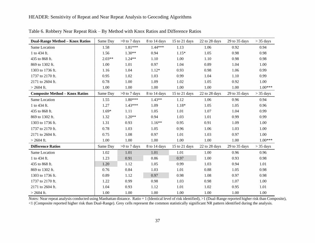
HEADER: Sensitivity of Repeat and Near Repeat Analysis to Geocoding Algorithms
37
Table 6. Robbery Near Repeat Risk – By Method with Knox Ratios and Difference Ratios
Dual-Range Method – Knox Ratios Same Day >0 to 7 days 8 to 14 days 15 to 21 days 22 to 28 days 29 to 35 days > 35 days
Same Location 1.58 1.81*** 1.44*** 1.13 1.06 0.92 0.94
1 to 434 ft. 1.56 1.30** 0.94 1.15* 1.05 0.98 0.98
435 to 868 ft. 2.03** 1.24** 1.10 1.00 1.10 0.98 0.98
869 to 1302 ft. 1.00 1.01 0.97 1.04 0.89 1.04 1.00
1303 to 1736 ft. 1.16 1.04 1.12* 0.93 0.98 1.06 0.99
1737 to 2170 ft. 0.95 1.02 1.03 0.99 1.04 1.10 0.99
2171 to 2604 ft. 0.78 1.00 1.09 1.02 1.05 0.92 1.00
> 2604 ft. 1.00 1.00 1.00 1.00 1.00 1.00 1.00***
Composite Method – Knox Ratios Same Day >0 to 7 days 8 to 14 days 15 to 21 days 22 to 28 days 29 to 35 days > 35 days
Same Location 1.55 1.80*** 1.43** 1.12 1.06 0.96 0.94
1 to 434 ft. 1.27 1.43*** 1.09 1.18* 1.05 1.05 0.96
435 to 868 ft. 1.69* 1.11 1.05 1.01 1.07 1.04 0.99
869 to 1302 ft. 1.32 1.20** 0.94 1.03 1.01 0.99 0.99
1303 to 1736 ft. 1.31 0.93 1.16** 0.95 0.91 1.09 1.00
1737 to 2170 ft. 0.78 1.03 1.05 0.96 1.06 1.03 1.00
2171 to 2604 ft. 0.75 1.08 0.97 1.01 1.03 0.97 1.00
> 2604 ft. 1.00 1.00 1.00 1.00 1.00 1.00 1.00***
Difference Ratios Same Day >0 to 7 days 8 to 14 days 15 to 21 days 22 to 28 days 29 to 35 days > 35 days
Same Location 1.02 1.01 1.01 1.01 1.00 0.96 0.96
1 to 434 ft. 1.23 0.91 0.86 0.97 1.00 0.93 0.98
435 to 868 ft. 1.20 1.12 1.05 0.99 1.03 0.94 1.01
869 to 1302 ft. 0.76 0.84 1.03 1.01 0.88 1.05 0.98
1303 to 1736 ft. 0.89 1.12 0.97 0.98 1.08 0.97 0.98
1737 to 2170 ft. 1.22 0.99 0.98 1.03 0.98 1.07 1.00
2171 to 2604 ft. 1.04 0.93 1.12 1.01 1.02 0.95 1.01
> 2604 ft. 1.00 1.00 1.00 1.00 1.00 1.00 1.00
Notes: Near repeat analysis conducted using Manhattan distance. Ratio = 1 (Identical level of risk identified), >1 (Dual-Range reported higher risk than Composite),
<1 (Composite reported higher risk than Dual-Range). Grey cells represent the common statistically significant NR pattern identified during the analysis.
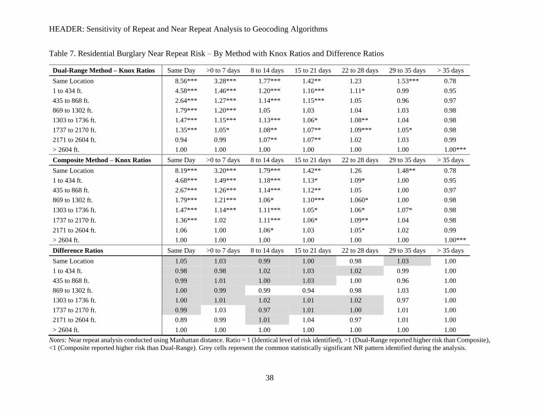
HEADER: Sensitivity of Repeat and Near Repeat Analysis to Geocoding Algorithms
38
Table 7. Residential Burglary Near Repeat Risk – By Method with Knox Ratios and Difference Ratios
Dual-Range Method – Knox Ratios Same Day >0 to 7 days 8 to 14 days 15 to 21 days 22 to 28 days 29 to 35 days > 35 days
Same Location 8.56*** 3.28*** 1.77*** 1.42** 1.23 1.53*** 0.78
1 to 434 ft. 4.58*** 1.46*** 1.20*** 1.16*** 1.11* 0.99 0.95
435 to 868 ft. 2.64*** 1.27*** 1.14*** 1.15*** 1.05 0.96 0.97
869 to 1302 ft. 1.79*** 1.20*** 1.05 1.03 1.04 1.03 0.98
1303 to 1736 ft. 1.47*** 1.15*** 1.13*** 1.06* 1.08** 1.04 0.98
1737 to 2170 ft. 1.35*** 1.05* 1.08** 1.07** 1.09*** 1.05* 0.98
2171 to 2604 ft. 0.94 0.99 1.07** 1.07** 1.02 1.03 0.99
> 2604 ft. 1.00 1.00 1.00 1.00 1.00 1.00 1.00***
Composite Method – Knox Ratios Same Day >0 to 7 days 8 to 14 days 15 to 21 days 22 to 28 days 29 to 35 days > 35 days
Same Location 8.19*** 3.20*** 1.79*** 1.42** 1.26 1.48** 0.78
1 to 434 ft. 4.68*** 1.49*** 1.18*** 1.13* 1.09* 1.00 0.95
435 to 868 ft. 2.67*** 1.26*** 1.14*** 1.12** 1.05 1.00 0.97
869 to 1302 ft. 1.79*** 1.21*** 1.06* 1.10*** 1.060* 1.00 0.98
1303 to 1736 ft. 1.47*** 1.14*** 1.11*** 1.05* 1.06* 1.07* 0.98
1737 to 2170 ft. 1.36*** 1.02 1.11*** 1.06* 1.09** 1.04 0.98
2171 to 2604 ft. 1.06 1.00 1.06* 1.03 1.05* 1.02 0.99
> 2604 ft. 1.00 1.00 1.00 1.00 1.00 1.00 1.00***
Difference Ratios Same Day >0 to 7 days 8 to 14 days 15 to 21 days 22 to 28 days 29 to 35 days > 35 days
Same Location 1.05 1.03 0.99 1.00 0.98 1.03 1.00
1 to 434 ft. 0.98 0.98 1.02 1.03 1.02 0.99 1.00
435 to 868 ft. 0.99 1.01 1.00 1.03 1.00 0.96 1.00
869 to 1302 ft. 1.00 0.99 0.99 0.94 0.98 1.03 1.00
1303 to 1736 ft. 1.00 1.01 1.02 1.01 1.02 0.97 1.00
1737 to 2170 ft. 0.99 1.03 0.97 1.01 1.00 1.01 1.00
2171 to 2604 ft. 0.89 0.99 1.01 1.04 0.97 1.01 1.00
> 2604 ft. 1.00 1.00 1.00 1.00 1.00 1.00 1.00
Notes: Near repeat analysis conducted using Manhattan distance. Ratio = 1 (Identical level of risk identified), >1 (Dual-Range reported higher risk than Composite),
<1 (Composite reported higher risk than Dual-Range). Grey cells represent the common statistically significant NR pattern identified during the analysis.
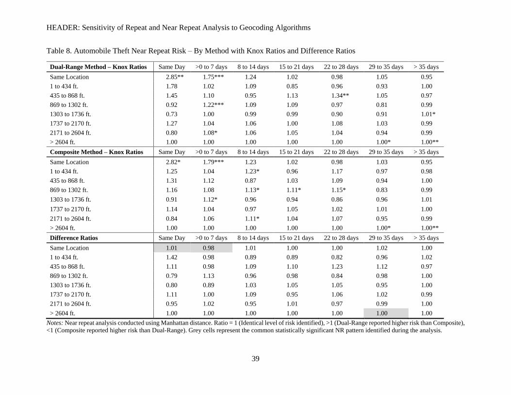
HEADER: Sensitivity of Repeat and Near Repeat Analysis to Geocoding Algorithms
39
Table 8. Automobile Theft Near Repeat Risk – By Method with Knox Ratios and Difference Ratios
Dual-Range Method – Knox Ratios Same Day >0 to 7 days 8 to 14 days 15 to 21 days 22 to 28 days 29 to 35 days > 35 days
Same Location 2.85** 1.75*** 1.24 1.02 0.98 1.05 0.95
1 to 434 ft. 1.78 1.02 1.09 0.85 0.96 0.93 1.00
435 to 868 ft. 1.45 1.10 0.95 1.13 1.34** 1.05 0.97
869 to 1302 ft. 0.92 1.22*** 1.09 1.09 0.97 0.81 0.99
1303 to 1736 ft. 0.73 1.00 0.99 0.99 0.90 0.91 1.01*
1737 to 2170 ft. 1.27 1.04 1.06 1.00 1.08 1.03 0.99
2171 to 2604 ft. 0.80 1.08* 1.06 1.05 1.04 0.94 0.99
> 2604 ft. 1.00 1.00 1.00 1.00 1.00 1.00* 1.00**
Composite Method – Knox Ratios Same Day >0 to 7 days 8 to 14 days 15 to 21 days 22 to 28 days 29 to 35 days > 35 days
Same Location 2.82* 1.79*** 1.23 1.02 0.98 1.03 0.95
1 to 434 ft. 1.25 1.04 1.23* 0.96 1.17 0.97 0.98
435 to 868 ft. 1.31 1.12 0.87 1.03 1.09 0.94 1.00
869 to 1302 ft. 1.16 1.08 1.13* 1.11* 1.15* 0.83 0.99
1303 to 1736 ft. 0.91 1.12* 0.96 0.94 0.86 0.96 1.01
1737 to 2170 ft. 1.14 1.04 0.97 1.05 1.02 1.01 1.00
2171 to 2604 ft. 0.84 1.06 1.11* 1.04 1.07 0.95 0.99
> 2604 ft. 1.00 1.00 1.00 1.00 1.00 1.00* 1.00**
Difference Ratios Same Day >0 to 7 days 8 to 14 days 15 to 21 days 22 to 28 days 29 to 35 days > 35 days
Same Location 1.01 0.98 1.01 1.00 1.00 1.02 1.00
1 to 434 ft. 1.42 0.98 0.89 0.89 0.82 0.96 1.02
435 to 868 ft. 1.11 0.98 1.09 1.10 1.23 1.12 0.97
869 to 1302 ft. 0.79 1.13 0.96 0.98 0.84 0.98 1.00
1303 to 1736 ft. 0.80 0.89 1.03 1.05 1.05 0.95 1.00
1737 to 2170 ft. 1.11 1.00 1.09 0.95 1.06 1.02 0.99
2171 to 2604 ft. 0.95 1.02 0.95 1.01 0.97 0.99 1.00
> 2604 ft. 1.00 1.00 1.00 1.00 1.00 1.00 1.00
Notes: Near repeat analysis conducted using Manhattan distance. Ratio = 1 (Identical level of risk identified), >1 (Dual-Range reported higher risk than Composite),
<1 (Composite reported higher risk than Dual-Range). Grey cells represent the common statistically significant NR pattern identified during the analysis.
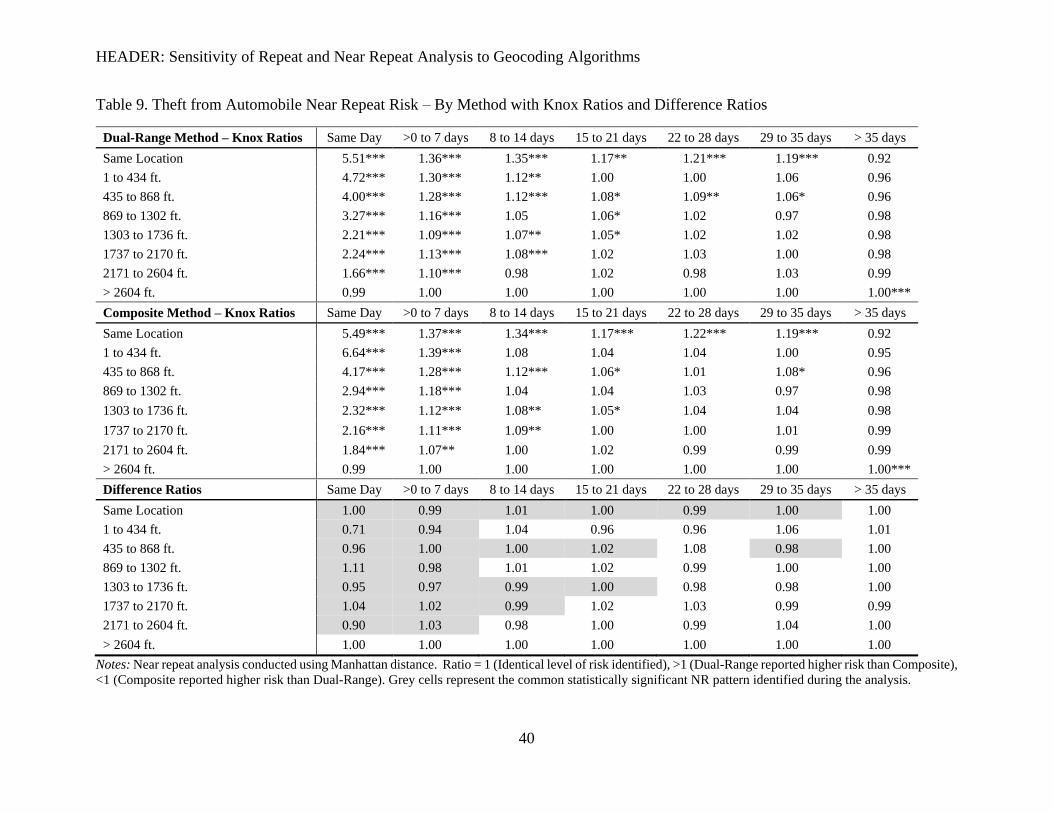
HEADER: Sensitivity of Repeat and Near Repeat Analysis to Geocoding Algorithms
40
Table 9. Theft from Automobile Near Repeat Risk – By Method with Knox Ratios and Difference Ratios
Dual-Range Method – Knox Ratios Same Day >0 to 7 days 8 to 14 days 15 to 21 days 22 to 28 days 29 to 35 days > 35 days
Same Location 5.51*** 1.36*** 1.35*** 1.17** 1.21*** 1.19*** 0.92
1 to 434 ft. 4.72*** 1.30*** 1.12** 1.00 1.00 1.06 0.96
435 to 868 ft. 4.00*** 1.28*** 1.12*** 1.08* 1.09** 1.06* 0.96
869 to 1302 ft. 3.27*** 1.16*** 1.05 1.06* 1.02 0.97 0.98
1303 to 1736 ft. 2.21*** 1.09*** 1.07** 1.05* 1.02 1.02 0.98
1737 to 2170 ft. 2.24*** 1.13*** 1.08*** 1.02 1.03 1.00 0.98
2171 to 2604 ft. 1.66*** 1.10*** 0.98 1.02 0.98 1.03 0.99
> 2604 ft. 0.99 1.00 1.00 1.00 1.00 1.00 1.00***
Composite Method – Knox Ratios Same Day >0 to 7 days 8 to 14 days 15 to 21 days 22 to 28 days 29 to 35 days > 35 days
Same Location 5.49*** 1.37*** 1.34*** 1.17*** 1.22*** 1.19*** 0.92
1 to 434 ft. 6.64*** 1.39*** 1.08 1.04 1.04 1.00 0.95
435 to 868 ft. 4.17*** 1.28*** 1.12*** 1.06* 1.01 1.08* 0.96
869 to 1302 ft. 2.94*** 1.18*** 1.04 1.04 1.03 0.97 0.98
1303 to 1736 ft. 2.32*** 1.12*** 1.08** 1.05* 1.04 1.04 0.98
1737 to 2170 ft. 2.16*** 1.11*** 1.09** 1.00 1.00 1.01 0.99
2171 to 2604 ft. 1.84*** 1.07** 1.00 1.02 0.99 0.99 0.99
> 2604 ft. 0.99 1.00 1.00 1.00 1.00 1.00 1.00***
Difference Ratios Same Day >0 to 7 days 8 to 14 days 15 to 21 days 22 to 28 days 29 to 35 days > 35 days
Same Location 1.00 0.99 1.01 1.00 0.99 1.00 1.00
1 to 434 ft. 0.71 0.94 1.04 0.96 0.96 1.06 1.01
435 to 868 ft. 0.96 1.00 1.00 1.02 1.08 0.98 1.00
869 to 1302 ft. 1.11 0.98 1.01 1.02 0.99 1.00 1.00
1303 to 1736 ft. 0.95 0.97 0.99 1.00 0.98 0.98 1.00
1737 to 2170 ft. 1.04 1.02 0.99 1.02 1.03 0.99 0.99
2171 to 2604 ft. 0.90 1.03 0.98 1.00 0.99 1.04 1.00
> 2604 ft. 1.00 1.00 1.00 1.00 1.00 1.00 1.00
Notes: Near repeat analysis conducted using Manhattan distance. Ratio = 1 (Identical level of risk identified), >1 (Dual-Range reported higher risk than Composite),
<1 (Composite reported higher risk than Dual-Range). Grey cells represent the common statistically significant NR pattern identified during the analysis.

The Sensitivity of Repeat and Near Repeat Analysis to Geocoding Algorithms
ONLINE APPENDIX
To save print space, this online appendix contains:
1. A table describing the repeat and near repeat analysis studies reviewed for this manuscript.
2. The results of the sensitivity check using Euclidean distance measures for the near repeat
analysis.
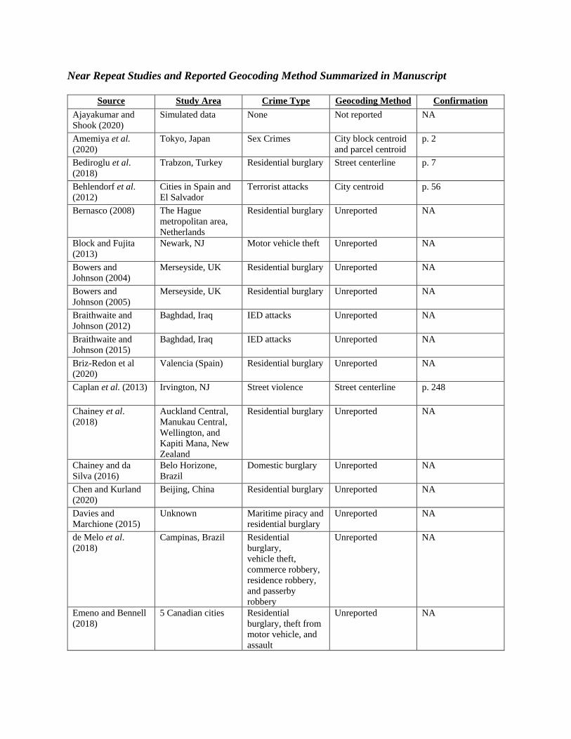
Near Repeat Studies and Reported Geocoding Method Summarized in Manuscript
Source Study Area Crime Type Geocoding Method Confirmation
Ajayakumar and
Shook (2020)
Simulated data None Not reported NA
Amemiya et al.
(2020)
Tokyo, Japan Sex Crimes City block centroid
and parcel centroid
p. 2
Bediroglu et al.
(2018)
Trabzon, Turkey Residential burglary Street centerline p. 7
Behlendorf et al.
(2012)
Cities in Spain and
El Salvador
Terrorist attacks City centroid p. 56
Bernasco (2008) The Hague
metropolitan area,
Netherlands
Residential burglary Unreported NA
Block and Fujita
(2013)
Newark, NJ Motor vehicle theft Unreported NA
Bowers and
Johnson (2004)
Merseyside, UK Residential burglary Unreported NA
Bowers and
Johnson (2005)
Merseyside, UK Residential burglary Unreported NA
Braithwaite and
Johnson (2012)
Baghdad, Iraq IED attacks Unreported NA
Braithwaite and
Johnson (2015)
Baghdad, Iraq IED attacks Unreported NA
Briz-Redon et al
(2020)
Valencia (Spain) Residential burglary Unreported NA
Caplan et al. (2013) Irvington, NJ Street violence Street centerline p. 248
Chainey et al.
(2018)
Auckland Central,
Manukau Central,
Wellington, and
Kapiti Mana, New
Zealand
Residential burglary Unreported NA
Chainey and da
Silva (2016)
Belo Horizone,
Brazil
Domestic burglary Unreported NA
Chen and Kurland
(2020)
Beijing, China Residential burglary Unreported NA
Davies and
Marchione (2015)
Unknown Maritime piracy and
residential burglary
Unreported NA
de Melo et al.
(2018)
Campinas, Brazil Residential
burglary,
vehicle theft,
commerce robbery,
residence robbery,
and passerby
robbery
Unreported NA
Emeno and Bennell
(2018)
5 Canadian cities Residential
burglary, theft from
motor vehicle, and
assault
Unreported NA
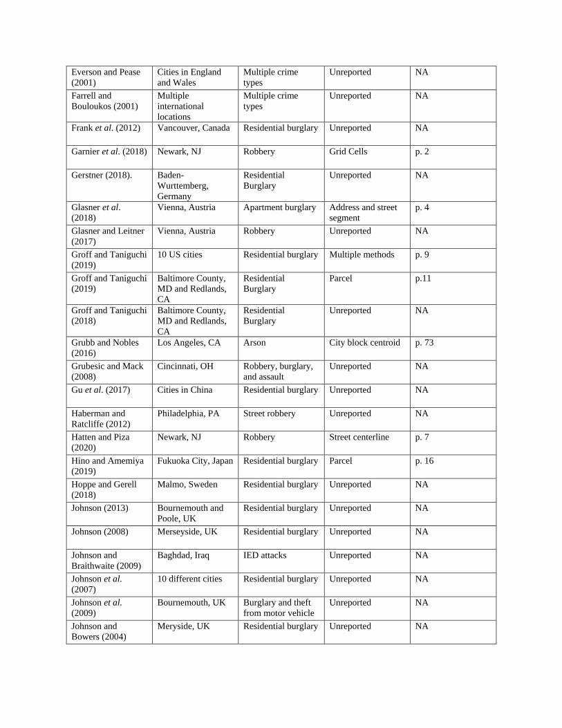
Everson and Pease
(2001)
Cities in England
and Wales
Multiple crime
types
Unreported NA
Farrell and
Bouloukos (2001)
Multiple
international
locations
Multiple crime
types
Unreported NA
Frank et al. (2012) Vancouver, Canada Residential burglary Unreported NA
Garnier et al. (2018) Newark, NJ Robbery Grid Cells p. 2
Gerstner (2018). Baden-
Wurttemberg,
Germany
Residential
Burglary
Unreported NA
Glasner et al.
(2018)
Vienna, Austria Apartment burglary Address and street
segment
p. 4
Glasner and Leitner
(2017)
Vienna, Austria Robbery Unreported NA
Groff and Taniguchi
(2019)
10 US cities Residential burglary Multiple methods p. 9
Groff and Taniguchi
(2019)
Baltimore County,
MD and Redlands,
CA
Residential
Burglary
Parcel p.11
Groff and Taniguchi
(2018)
Baltimore County,
MD and Redlands,
CA
Residential
Burglary
Unreported NA
Grubb and Nobles
(2016)
Los Angeles, CA Arson City block centroid p. 73
Grubesic and Mack
(2008)
Cincinnati, OH Robbery, burglary,
and assault
Unreported NA
Gu et al. (2017) Cities in China Residential burglary Unreported NA
Haberman and
Ratcliffe (2012)
Philadelphia, PA Street robbery Unreported NA
Hatten and Piza
(2020)
Newark, NJ Robbery Street centerline p. 7
Hino and Amemiya
(2019)
Fukuoka City, Japan Residential burglary Parcel p. 16
Hoppe and Gerell
(2018)
Malmo, Sweden Residential burglary Unreported NA
Johnson (2013) Bournemouth and
Poole, UK
Residential burglary Unreported NA
Johnson (2008) Merseyside, UK Residential burglary Unreported NA
Johnson and
Braithwaite (2009)
Baghdad, Iraq IED attacks Unreported NA
Johnson et al.
(2007)
10 different cities Residential burglary Unreported NA
Johnson et al.
(2009)
Bournemouth, UK Burglary and theft
from motor vehicle
Unreported NA
Johnson and
Bowers (2004)
Meryside, UK Residential burglary Unreported NA
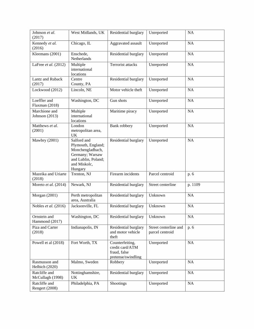
Johnson et al.
(2017)
West Midlands, UK Residential burglary Unreported NA
Kennedy et al.
(2016)
Chicago, IL Aggravated assault Unreported NA
Kleemans (2001) Enschede,
Netherlands
Residential burglary Unreported NA
LaFree et al. (2012) Multiple
international
locations
Terrorist attacks Unreported NA
Lantz and Ruback
(2017)
Centre
County, PA
Residential burglary Unreported NA
Lockwood (2012) Lincoln, NE Motor vehicle theft Unreported NA
Loeffler and
Flaxman (2018)
Washington, DC Gun shots Unreported NA
Marchione and
Johnson (2013)
Multiple
international
locations
Maritime piracy Unreported NA
Matthews et al.
(2001)
London
metropolitan area,
UK
Bank robbery Unreported NA
Mawbry (2001) Salford and
Plymouth, England;
Monchengladbach,
Germany; Warsaw
and Lublin, Poland;
and Miskolc,
Hungary
Residential burglary Unreported NA
Mazeika and Uriarte
(2018)
Trenton, NJ Firearm incidents Parcel centroid p. 6
Moreto et al. (2014) Newark, NJ Residential burglary Street centerline p. 1109
Morgan (2001) Perth metropolitan
area, Australia
Residential burglary Unknown NA
Nobles et al. (2016) Jacksonville, FL Residential burglary Unknown NA
Ornstein and
Hammond (2017)
Washington, DC Residential burglary Unknown NA
Piza and Carter
(2018)
Indianapolis, IN Residential burglary
and motor vehicle
theft
Street centerline and
parcel centroid
p. 6
Powell et al (2018) Fort Worth, TX Counterfeiting,
credit card/ATM
fraud, false
pretense/swindling
Unreported NA
Rasmusson and
Helbich (2020)
Malmo, Sweden Robbery Unreported NA
Ratcliffe and
McCullagh (1998)
Nottinghamshire,
UK
Residential burglary Unreported NA
Ratcliffe and
Rengert (2008)
Philadelphia, PA Shootings Unreported NA
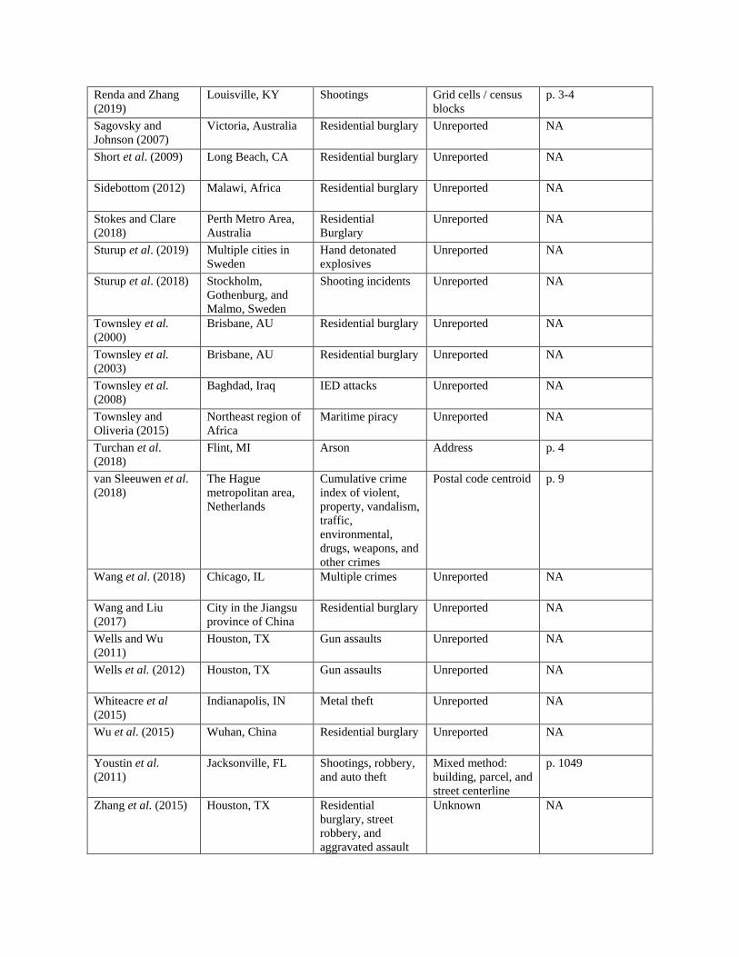
Renda and Zhang
(2019)
Louisville, KY Shootings Grid cells / census
blocks
p. 3-4
Sagovsky and
Johnson (2007)
Victoria, Australia Residential burglary Unreported NA
Short et al. (2009) Long Beach, CA Residential burglary Unreported NA
Sidebottom (2012) Malawi, Africa Residential burglary Unreported NA
Stokes and Clare
(2018)
Perth Metro Area,
Australia
Residential
Burglary
Unreported NA
Sturup et al. (2019) Multiple cities in
Sweden
Hand detonated
explosives
Unreported NA
Sturup et al. (2018) Stockholm,
Gothenburg, and
Malmo, Sweden
Shooting incidents Unreported NA
Townsley et al.
(2000)
Brisbane, AU Residential burglary Unreported NA
Townsley et al.
(2003)
Brisbane, AU Residential burglary Unreported NA
Townsley et al.
(2008)
Baghdad, Iraq IED attacks Unreported NA
Townsley and
Oliveria (2015)
Northeast region of
Africa
Maritime piracy Unreported NA
Turchan et al.
(2018)
Flint, MI Arson Address p. 4
van Sleeuwen et al.
(2018)
The Hague
metropolitan area,
Netherlands
Cumulative crime
index of violent,
property, vandalism,
traffic,
environmental,
drugs, weapons, and
other crimes
Postal code centroid p. 9
Wang et al. (2018) Chicago, IL Multiple crimes Unreported NA
Wang and Liu
(2017)
City in the Jiangsu
province of China
Residential burglary Unreported NA
Wells and Wu
(2011)
Houston, TX Gun assaults Unreported NA
Wells et al. (2012) Houston, TX Gun assaults Unreported NA
Whiteacre et al
(2015)
Indianapolis, IN Metal theft Unreported NA
Wu et al. (2015) Wuhan, China Residential burglary Unreported NA
Youstin et al.
(2011)
Jacksonville, FL Shootings, robbery,
and auto theft
Mixed method:
building, parcel, and
street centerline
p. 1049
Zhang et al. (2015) Houston, TX Residential
burglary, street
robbery, and
aggravated assault
Unknown NA
Full Reference Details for the Studies Listed Above
1. Ajayakumar, J. & Shook, E. (2020). Leveraging parallel spatio-temporal computing for crime
analysis in large datasets: analyzing trends in near-repeat phenomenon of crime in cities.
International Journal of Geographical Information Science. Online First.
https://doi.org/10.1080/13658816.2020.1732393
2. Amemiya, M., Nakaya, T., & Shimada, T. (2020). Near-repeat victimization of sex crimes
and threat incidents against women and girls in Tokyo, Japan. Crime Science, 9(5), 1-6.
3. Bediroglu, G., Bediroglu, S., Colak, H. E., & Yomralioglu, T. (2018). A crime prevention
system in spatiotemporal principles with repeat, near-repeat analysis, and crime density
mapping: Case study Turkey, Trabzon. Crime & Delinquency. Online First. DOI:
10.1177/0011128717750391
4. Behlendorf, B., LaFree, G., & Legault, R. (2012). Microcycles of violence: Evidence from
terrorist attacks by ETA and the FMLN. Journal of Quantitative Criminology, 28(1), 49-75.
5. Bernasco, W. (2008). Them again? Same-offender involvement in repeat and near repeat
burglaries. European Journal of Criminology, 5(4), 411-431.
6. Block, S., & Fujita, S. (2013). Patterns of near repeat temporary and permanent motor
vehicles thefts. Crime Prevention and Community Safety, 15(2), 151-167.
7. Bowers, K. J., & Johnson, S. D. (2004). Who commits near repeats? A test of the boost
explanation. Western Criminology Review, 5(3), 12-24.
8. Bowers, K. J., & Johnson, S. D. (2005). Domestic burglary repeats and space-time clusters:
The dimensions of risk. European Journal of Criminology, 2(1), 67-92.
9. Braithwaite, A., & Johnson, S. D. (2012). Space-time modeling of insurgency and
counterinsurgency in Iraq. Journal of Quantitative Criminology, 28(1), 31-48.
10. Braithwaite, A., & Johnson, S. D. (2015). The battle for Baghdad: Testing hypotheses about
insurgency from risk heterogeneity, repeat victimization, and denial policing approaches.
Terrorism and Political Violence, 27(1), 112-132.
11. Briz-Redon, A., Martinez-Ruiz, F., & Montes, F. (2020). Adjusting the Knox test by
accounting for spatiotemporal crime risk heterogeneity to analyze near-repeats. European
Journal of Criminology. Online first. DOI: 10.1177/1477370820905106
12. Caplan, J., Kennedy, L., & Piza, E. (2013). Joint utility of event dependent and contextual
crime analysis techniques for violent crime forecasting. Crime & Delinquency, 59(2), 243-
270.
13. Chainey, S. P., Curtis-Ham, S. J., Evans, R. M., & Burns, G. J. (2018). Examining the extent
to which repeat and near repeat patterns can prevent crime. Policing: An International
Journal of Police Strategies & Management. Online First. https://doi.org/10.1108/PIJPSM-
12-2016-0172
14. Chainey, S. P., & da Silva, B. F. A. (2016). Examining the extent of repeat and near repeat
victimization of domestic burglaries in Belo Horizonte, Brazil. Crime Science, 5(1). DOI
10.1186/s40163-016-0049-6
15. Chen, P., & Kurland, J. (2020). The impact of “stroke hard” on repeat and near-repeat
residential burglary. International Journal of Geo-Information, 9, 150.
doi:10.3390/ijgi9030150
16. Davies, T. & Marchione, E. (2015). Event networks and the identification of crime pattern
motifs. PLoS ONE, 10(11), 1-19. e0143638. https://doi.org/10.1371/journal.pone.0143638
17. de Melo, S. N., Andresen, M. A., Matias, L. F. (2018). Repeat and near-repeat victimization
in Campinas, Brazil: New explanations from the global south. Security Journal, 31(1), 364-
38.
18. Emeno, K., & Bennell, C. (2018). Near repeat space-time patterns of Canadian crime.
Canadian Journal of Criminology and Criminal Justice, 60(2), 141-166.
19. Everson, S., & Pease, K. (2001). Crime against the same person and place: Detection
opportunity and offender targeting. Crime Prevention Studies, 12, 199-220.
20. Farrell, G., & Bouloukos, A. C. (2001). International overview: A cross-national comparison
of rates of repeat victimization. Crime Prevention Studies, 12, 5-25.
21. Frank, R., Brantingham, P., & Farrell, G. (2012). Estimating the true rate of repeat
victimization from police record crime data: A study of burglary in metro Vancouver.
Canadian Journal of Criminology and Criminal Justice, 54(4), 481-494.
22. Garnier, S., Caplan, J. M., & Kennedy, L. W. (2018). Predicting dynamical crime distribution
from environmental and social influences. Frontiers in Applied Mathematics and Statistics,
4(13). doi: 10.3389/fams.2018.00013
23. Gerstner, D. (2018). Predictive policing in the context of residential burglary: an empirical
illustration on the basis of a pilot project in Baden-Wurttemberg, Germany. European
Journal for Security Research. Online First. https://doi.org/10.1007/s41125-018-0033-0
24. Glasner, P., Johnson, S. D., & Leitner, M. (2018). A comparative analysis to forecast
apartment burglaries in Vienna, Austria, based on repeat and near repeat victimization. Crime
Science, 7(9), https://doi.org/10.1186/s40163-018-0083-7
25. Glasner, P., & Leitner, M. (2017). Evaluating the impact the weekday has on near-repeat
victimization: A spatio-temporal analysis of street robberies in the city of Vienna, Austria.
International Journal of Geo-Information, 6(3), doi:10.3390/ijgi6010003
26. Groff, E. R., & Taniguchi, T. A. (2019). Quantifying crime prevention potential of near-
repeat burglary. Police Quarterly. Online First. DOI: 10.1177/1098611119828052
27. Groff, E. R., & Taniguchi, T. A. (2019). Using citizen notification to interrupt near-repeat
residential burglary patterns: the micro-level near-repeat experiment. Journal of
Experimental Criminology. Online First. https://doi.org/10.1007/s11292-018-09350-1
28. Groff, E. R., & Taniguchi, T. A. (2018). Micro-Level Policing for Preventing Near Repeat
Residential Burglary. Technical Report. Police Foundation.
29. Grubb, J. A., & Nobles, M. R. (2016). A spatiotemporal analysis of arson. Journal of
Research in Crime and Delinquency, 53(1), 66-92.
30. Grubesic, T., & Mack, E. (2008). Spatio-temporal interaction of urban crime. Journal of
Quantitative Criminology, 24(3), 285-306.
31. Gu, Y., Wang, Q., & Yi, G. (2017). Stationary patterns and their selection mechanism of
urban crime models with heterogeneous near-repeat victimization effect. European Journal
of Applied Mathematics, 28(1), 141-178.
32. Haberman, C., & Ratcliffe, J. H. (2012). The predictive policing challenges of near repeat
armed street robberies. Policing: A Journal of Policy and Practice, 6(2), 151-166.
33. Hatten, D. & Piza, E. (2020). Measuring the Temporal Stability of Near-Repeat Crime
Patterns: A Longitudinal Analysis. Crime & Delinquency. DOI: 10.1177/0011128720922545.
34. Hino, K. & Amemiya, M. (2019). Spatiotemporal analysis of burglary in multifamily housing
in Fukuoka City, Japan. Cities, 90, 15-23.
35. Hoppe, L., & Gerell, M. (2018). Near repeat burglary patterns in Malmo: Stability and
change over time. European Journal of Criminology. Online First. DOI:
10.1177/1477370817751382
36. Johnson, D. (2013). The space/time behavior of dwelling burglars: Finding near repeat
patterns in serial offender data. Applied Geography, 41, 139-146.
37. Johnson, S. D. (2008). Repeat burglary victimization: A tale of two theories. Journal of
Experimental Criminology, 4(3), 215-240.
38. Johnson, S. D., Bernasco, W., Bowers, K., Elffers, H., Ratcliffe, J., Rengert, G., & Townsley,
M. (2007). Space-time patterns of risk: A cross national assessment of residential burglary
victimization. Journal of Quantitative Criminology, 23(3), 201-219.
39. Johnson, S., & Bowers, K. (2004). The burglary as clue to the future: The beginning of
prospective hot spotting. European Journal of Criminology, 1(2), 237-255.
40. Johnson, S. D., & Braithwaite, A. (2009). Spatio-temporal modeling of insurgency in Iraq.
Crime Prevention Studies, 25, 9-32.
41. Johnson, S. D., Davies, T., Murray, A., Ditta, P., Belur, J., & Bowers, K. (2017). Evaluation
of operation swordfish: A near repeat target-hardening strategy. Journal of Experimental
Criminology, 13(4), 505-525.
42. Johnson, S. D., Summers, L., & Pease, K. (2009). Offender as forager? A direct test of the
boost account of victimization. Journal of Quantitative Criminology, 25(2), 181-200.
43. Kennedy, L., Caplan, J., Piza, E., & Buccine-Schraeder, H. (2016). Vulnerability and
exposure to crime: Applying risk terrain modeling to the study of assault in Chicago. Applied
Spatial Analysis and Policy, 9(4), 529-548.
44. Kleemans, E. R. (2001). Repeat burglary victimization: Results of empirical research in the
Netherlands. Crime Prevention Studies, 12, 53-68.
45. LaFree, G., Dugan, L., Xie, M., & Singh, P. (2012). Spatial and temporal patterns of terrorist
attacks by ETA 1970 to 2007. Journal of Quantitative Criminology, 28(1), 7-29.
46. Lantz, B., & Ruback, R. B. (2017). A networked boost: Burglary co-offending and repeat
victimization using a network approach. Crime & Delinquency, 63(9), 1066-1090.
47. Lockwood, B. (2012). The presence and nature of a near-repeat pattern of motor vehicle
theft. Security Journal, 25(1), 38-56.
48. Loeffler, C., & Flaxman, S. (2018). Is gun violence contagious? A spatiotemporal test.
Journal of Quantitative Criminology. Online First. DOI 10.1007/s10940-017-9363-8
49. Marchione, E. & Johnson, S. D. (2013). Spatial, temporal, and spatio-temporal patterns of
maritime piracy. Journal of Research in Crime and Delinquency, 50(4), 504-524.
50. Matthews, R., Pease, C., & Pease, K. (2001). Repeated bank robberies: Theme and
variations. Crime Prevention Studies, 12, 153-164.
51. Mawbry, R. I. (2001). The impact of repeat victimization on burglary victims in east and
west Europe. Crime Prevention Studies, 12, 69-82.
52. Mazeika, D. M., & Uriarte, L. (2018). The near repeats of gun violence using acoustic
triangulation data. Security Journal. Online First. https://doi.org/10.1057/s41284-018-0154-1
53. Moreto, W., Piza, E., & Caplan, J. (2014). A plague on both your houses? Risks, repeats, and
reconsiderations of urban residential burglary. Justice Quarterly, 31(6), 1102-1126.
54. Morgan, F. (2001). Repeat burglary in a Perth suburb: indicator of short-term or long-term
risk? Crime Prevention Studies, 12, 83-118.
55. Nobles, M., Ward, J., & Tillyer, R. (2016). The impact of neighborhood context on
spatiotemporal patterns of burglary. Journal of Research in Crime and Delinquency, 53(5),
711-740.
56. Ornstein, J. T., & Hammond, R. A. (2017). The burglary boost: A note on detecting
contagion using the Knox test. Journal of Quantitative Criminology, 33(1), 65-75.
57. Piza, E. L., & Carter, J. G. (2018). Predicting initiator and near repeat events in
spatiotemporal crime patterns: An analysis of residential burglary and motor vehicle theft.
Justice Quarterly, 35(5), 842-870. DOI: 10.1080/07418825.2017.1342854.
58. Powell, Z. A., Grubbs, J. A., & Nobles, M. R. (2018). A near repeat examination of
economic crime. Crime & Delinquency. Online First.
https://doi.org/10.1177/0011128718811927
59. Rasmusson, M. & Helbich, M. (2020). The relationship between near-repeat street robbery
and the environment: Evidence from Malo, Sweden. International Journal of Geo-
Information, 9, 188.
60. Ratcliffe, J. H., & McCullagh, M. J. (1998). Identifying repeat victimization with GIS.
British Journal of Criminology, 38(4), 651-662.
61. Ratcliffe, J. H., & Rengert, G. (2008). Near-repeat patterns in Philadelphia shootings.
Security Journal, 21(1), 58-76.
62. Renda, W., & Zhang, C. H. (2019). Comparative analysis of firearm discharge recorded by
gunshot detection technology and calls for service in Louisville, Kentucky. International
Journal of Geo-Information, 8(6), 275-291.
63. Sagovsky, A., & Johnson, S. D. (2007). When does repeat burglary victimization occur? The
Australian and New Zealand Journal of Criminology, 40(1), 1-26.
64. Short, M. B., D’Orsogna, M. R., Brantingham, P. J., & Tita, G. (2009). Measuring and
modeling repeat and near-repeat burglary effects. Journal of Quantitative Criminology,
25(3), 325-339.
65. Sidebottom, A. (2012). Repeat burglary victimization in Malawi and the influence of housing
type and area-level affluence. Security Journal, 25(3), 265-281.
66. Stokes, N., & Clare, J. (2018). Preventing near-repeat residential burglary through
cocooning: post hoc evaluation of a targeted police-led pilot intervention. Security Journal.
Online First. https://doi.org/10.1057/s41284-018-0144-3
67. Sturup, J., Gerell, M., & Rostami, A. (2019). Explosive violence: A near-repeat study of
hand grenade detonations and shootings in urban Sweden. European Journal of Criminology.
Online First. https://doi.org/10.1177/1477370818820656
68. Sturup, J., Rostami, A., Gerell, M., & Sandholm, A. (2018). Near-repeat shootings in
contemporary Sweden 2011 to 2015. Security Journal, 31(1), 73-92.
69. Townsley, M., Homel, R., & Chaselin, J. (2000). Repeat burglary victimization: Spatial and
temporal patterns. The Australian and New Zealand Journal of Criminology, 33(1), 37-63.
70. Townsley, M., Homel, R., & Chaselin, J. (2003). Infectious burglaries. A test of the near
repeat hypothesis. British Journal of Criminology, 43(3), 615-633.
71. Townsley, M., Johnson, S., & Ratcliffe, J. (2008). Space-time dynamics of insurgent activity
in Iraq. Security Journal, 21(3), 139-146.
72. Townsley, M., & Oliveira, A. (2015). Space-time dynamics of maritime piracy. Security
Journal, 28(3), 217-229.
73. Turchan, B., Grubb, J. A., Pizarro, J. M., & McGarrell, E. F. (2018). Arson in an urban
setting: a multi‑event near repeat chain analysis in Flint, Michigan. Security Journal. Online
First. https://doi.org/10.1057/s41284-018-0155-0
74. van Sleeuwen, S. E. M., Ruiter, S., & Menting, B. (2018). A time for a crime: Temporal
aspects of repeat offenders’ crime location choices. Journal of Research in Crime and
Delinquency. Online First. DOI: 10.1177/0022427818766395
75. Wang, K., Cai, Z., Zhu, P., Cui, P., Zhu, H., & Li, Y. (2018). Adopting data interpretation on
mining fine-grained near-repeat patterns in crimes. Journal of Forensic and Legal Medicine,
55, 76-86.
76. Wang, Z., & Liu, X. (2017). Analysis of burglary hot spots and near-repeat victimization in a
large Chinese city. International Journal of Geo-Information, 6(5), doi:10.3390/ijgi6050148
77. Wells, W., & Wu, L. (2011). Proactive policing effects on repeat and near-repeat shootings in
Houston. Police Quarterly, 14(3), 298-319.
78. Wells, W., Wu, L., & Ye, W. (2012). Patterns of near-repeat gun assaults in Houston.
Journal of Research in Crime and Delinquency, 49(2), 186-212.
79. Whiteacre, K., Terheide, D., & Biggs, B. (2015). Metal theft and repeat victimization. Crime
Prevention and Community Safety, 17(3), 139-155.
80. Wu, L., Xu, X., Ye, X., & Zhu, W. (2015). Repeat and near-repeat burglaries and offender
involvement in a large Chinese city. Cartography and Geographic Information Science,
42(2), 178-189.
81. Youstin, T., Nobles, M., Ward, J., & Cook, C. (2011). Assessing the generalizability of the
near repeat phenomenon. Criminal Justice and Behavior, 38(10), 1042-1063.
82. Zhang, Y., Zhao, J., Ren, L., & Hoover, L. (2015). Space-time clustering of crime events and
neighborhood characteristics in Houston. Criminal Justice Review, 40(3), 340-360.
Sensitivity Check Using Euclidean Distance
The results of all analyses in the manuscript were recomputed using Euclidean distance as
the distance measurement technique. Overall, the results are not sensitive to the distance
measurement technique chosen. In fact, in most instances, the results using Euclidean distance
show even fewer divergences than the results obtained using Manhattan distance that were
presented in the main body of the manuscript. We present these analyses in this online appendix
for the sake of transparency.
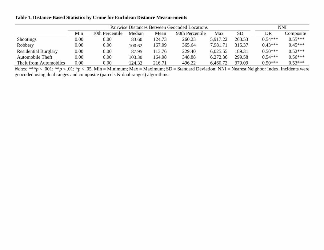
Table 1. Distance-Based Statistics by Crime for Euclidean Distance Measurements
Pairwise Distances Between Geocoded Locations NNI
Min 10th Percentile Median Mean 90th Percentile Max SD DR Composite
Shootings 0.00 0.00 83.60 124.73 260.23 5,917.22 263.53 0.54*** 0.55***
Robbery 0.00 0.00 100.62 167.09 365.64 7,981.71 315.37 0.43*** 0.45***
Residential Burglary 0.00 0.00 87.95 113.76 229.40 6,025.55 189.31 0.50*** 0.52***
Automobile Theft 0.00 0.00 103.30 164.98 348.88 6,272.36 299.58 0.54*** 0.56***
Theft from Automobiles 0.00 0.00 124.33 216.71 496.22 6,460.72 379.09 0.50*** 0.53***
Notes: ***p < .001; **p < .01; *p < .05. Min = Minimum; Max = Maximum; SD = Standard Deviation; NNI = Nearest Neighbor Index. Incidents were
geocoded using dual ranges and composite (parcels & dual ranges) algorithms.
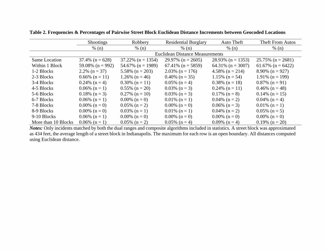
Table 2. Frequencies & Percentages of Pairwise Street Block Euclidean Distance Increments between Geocoded Locations
Shootings Robbery Residential Burglary Auto Theft Theft From Autos
% (n) % (n) % (n) % (n) % (n)
Euclidean Distance Measurements
Same Location 37.4% (n = 628) 37.22% (n = 1354) 29.97% (n = 2605) 28.93% (n = 1353) 25.75% (n = 2681)
Within 1 Block 59.08% (n = 992) 54.67% (n = 1989) 67.41% (n = 5859) 64.31% (n = 3007) 61.67% (n = 6422)
1-2 Blocks 2.2% (n = 37) 5.58% (n = 203) 2.03% (n = 176) 4.58% (n = 214) 8.90% (n = 927)
2-3 Blocks 0.66% (n = 11) 1.26% (n = 46) 0.40% (n = 35) 1.15% (n = 54) 1.91% (n = 199)
3-4 Blocks 0.24% (n = 4) 0.30% (n = 11) 0.05% (n = 4) 0.38% (n = 18) 0.87% (n = 91)
4-5 Blocks 0.06% (n = 1) 0.55% (n = 20) 0.03% (n = 3) 0.24% (n = 11) 0.46% (n = 48)
5-6 Blocks 0.18% (n = 3) 0.27% (n = 10) 0.03% (n = 3) 0.17% (n = 8) 0.14% (n = 15)
6-7 Blocks 0.06% (n = 1) 0.00% (n = 0) 0.01% (n = 1) 0.04% (n = 2) 0.04% (n = 4)
7-8 Blocks 0.00% (n = 0) 0.05% (n = 2) 0.00% (n = 0) 0.06% (n = 3) 0.01% (n = 1)
8-9 Blocks 0.00% (n = 0) 0.03% (n = 1) 0.01% (n = 1) 0.04% (n = 2) 0.05% (n = 5)
9-10 Blocks 0.06% (n = 1) 0.00% (n = 0) 0.00% (n = 0) 0.00% (n = 0) 0.00% (n = 0)
More than 10 Blocks 0.06% (n = 1) 0.05% (n = 2) 0.05% (n = 4) 0.09% (n = 4) 0.19% (n = 20)
Notes: Only incidents matched by both the dual ranges and composite algorithms included in statistics. A street block was approximated
as 434 feet, the average length of a street block in Indianapolis. The maximum for each row is an open boundary. All distances computed
using Euclidean distance.
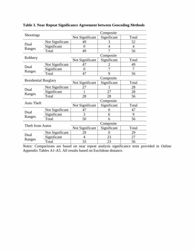
Table 3. Near Repeat Significance Agreement between Geocoding Methods
Shootings Composite
Not Significant Significant Total
Dual
Ranges
Not Significant 49 3 52
Significant 0 4 4
Total 49 7 56
Robbery Composite
Not Significant Significant Total
Dual
Ranges
Not Significant 47 2 49
Significant 0 7 7
Total 47 9 56
Residential Burglary Composite
Not Significant Significant Total
Dual
Ranges
Not Significant 27 1 28
Significant 1 27 28
Total 28 28 56
Auto Theft Composite
Not Significant Significant Total
Dual
Ranges
Not Significant 47 0 47
Significant 3 6 9
Total 50 6 56
Theft from Autos Composite
Not Significant Significant Total
Dual
Ranges
Not Significant 29 0 29
Significant 4 23 27
Total 33 23 56
Notes: Comparisons are based on near repeat analysis significance tests provided in Online
Appendix Tables A1-A5. All results based on Euclidean distance.
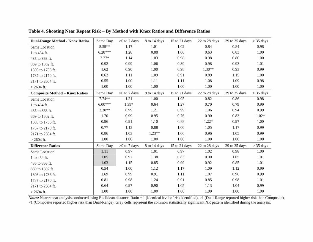
Table 4. Shooting Near Repeat Risk – By Method with Knox Ratios and Difference Ratios
Dual-Range Method - Knox Ratios Same Day >0 to 7 days 8 to 14 days 15 to 21 days 22 to 28 days 29 to 35 days > 35 days
Same Location 8.59** 1.17 1.01 1.02 0.84 0.84 0.98
1 to 434 ft. 6.28*** 1.28 0.88 1.06 0.63 0.83 1.00
435 to 868 ft. 2.27* 1.14 1.03 0.98 0.98 0.80 1.00
869 to 1302 ft. 0.92 0.99 1.06 0.89 0.98 0.93 1.01
1303 to 1736 ft. 1.62 0.90 1.00 0.98 1.30** 0.93 0.99
1737 to 2170 ft. 0.62 1.11 1.09 0.91 0.89 1.15 1.00
2171 to 2604 ft. 0.55 1.00 1.11 1.11 1.08 1.09 0.98
> 2604 ft. 1.00 1.00 1.00 1.00 1.00 1.00 1.00
Composite Method – Knox Ratios Same Day >0 to 7 days 8 to 14 days 15 to 21 days 22 to 28 days 29 to 35 days > 35 days
Same Location 7.74** 1.21 1.00 1.05 0.82 0.86 0.98
1 to 434 ft. 6.00*** 1.39* 0.64 1.27 0.70 0.79 0.99
435 to 868 ft. 2.20** 0.99 1.21 0.99 1.06 0.94 0.99
869 to 1302 ft. 1.70 0.99 0.95 0.76 0.90 0.83 1.02*
1303 to 1736 ft. 0.96 0.91 1.10 0.88 1.22* 0.97 1.00
1737 to 2170 ft. 0.77 1.13 0.88 1.00 1.05 1.17 0.99
2171 to 2604 ft. 0.86 1.03 1.23** 1.06 0.96 1.05 0.99
> 2604 ft. 1.00 1.00 1.00 1.00 1.00 1.00 1.00
Difference Ratios Same Day >0 to 7 days 8 to 14 days 15 to 21 days 22 to 28 days 29 to 35 days > 35 days
Same Location 1.11 0.97 1.01 0.97 1.02 0.98 1.00
1 to 434 ft. 1.05 0.92 1.38 0.83 0.90 1.05 1.01
435 to 868 ft. 1.03 1.15 0.85 0.99 0.92 0.85 1.01
869 to 1302 ft. 0.54 1.00 1.12 1.17 1.09 1.12 0.99
1303 to 1736 ft. 1.69 0.99 0.91 1.11 1.07 0.96 0.99
1737 to 2170 ft. 0.81 0.98 1.24 0.91 0.85 0.98 1.01
2171 to 2604 ft. 0.64 0.97 0.90 1.05 1.13 1.04 0.99
> 2604 ft. 1.00 1.00 1.00 1.00 1.00 1.00 1.00
Notes: Near repeat analysis conducted using Euclidean distance. Ratio = 1 (Identical level of risk identified), >1 (Dual-Range reported higher risk than Composite),
<1 (Composite reported higher risk than Dual-Range). Grey cells represent the common statistically significant NR pattern identified during the analysis.
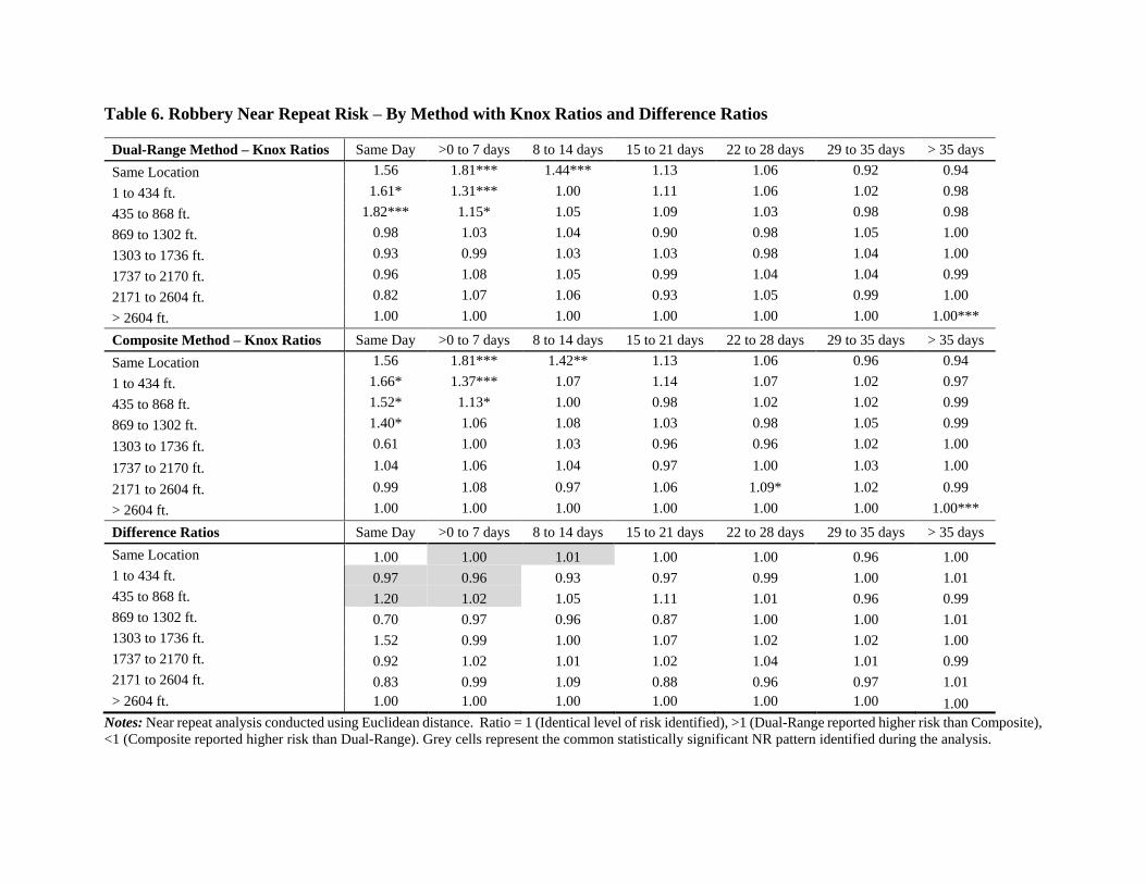
Table 6. Robbery Near Repeat Risk – By Method with Knox Ratios and Difference Ratios
Dual-Range Method – Knox Ratios Same Day >0 to 7 days 8 to 14 days 15 to 21 days 22 to 28 days 29 to 35 days > 35 days
Same Location 1.56 1.81*** 1.44*** 1.13 1.06 0.92 0.94
1 to 434 ft. 1.61* 1.31*** 1.00 1.11 1.06 1.02 0.98
435 to 868 ft. 1.82*** 1.15* 1.05 1.09 1.03 0.98 0.98
869 to 1302 ft. 0.98 1.03 1.04 0.90 0.98 1.05 1.00
1303 to 1736 ft. 0.93 0.99 1.03 1.03 0.98 1.04 1.00
1737 to 2170 ft. 0.96 1.08 1.05 0.99 1.04 1.04 0.99
2171 to 2604 ft. 0.82 1.07 1.06 0.93 1.05 0.99 1.00
> 2604 ft. 1.00 1.00 1.00 1.00 1.00 1.00 1.00***
Composite Method – Knox Ratios Same Day >0 to 7 days 8 to 14 days 15 to 21 days 22 to 28 days 29 to 35 days > 35 days
Same Location 1.56 1.81*** 1.42** 1.13 1.06 0.96 0.94
1 to 434 ft. 1.66* 1.37*** 1.07 1.14 1.07 1.02 0.97
435 to 868 ft. 1.52* 1.13* 1.00 0.98 1.02 1.02 0.99
869 to 1302 ft. 1.40* 1.06 1.08 1.03 0.98 1.05 0.99
1303 to 1736 ft. 0.61 1.00 1.03 0.96 0.96 1.02 1.00
1737 to 2170 ft. 1.04 1.06 1.04 0.97 1.00 1.03 1.00
2171 to 2604 ft. 0.99 1.08 0.97 1.06 1.09* 1.02 0.99
> 2604 ft. 1.00 1.00 1.00 1.00 1.00 1.00 1.00***
Difference Ratios Same Day >0 to 7 days 8 to 14 days 15 to 21 days 22 to 28 days 29 to 35 days > 35 days
Same Location 1.00 1.00 1.01 1.00 1.00 0.96 1.00
1 to 434 ft. 0.97 0.96 0.93 0.97 0.99 1.00 1.01
435 to 868 ft. 1.20 1.02 1.05 1.11 1.01 0.96 0.99
869 to 1302 ft. 0.70 0.97 0.96 0.87 1.00 1.00 1.01
1303 to 1736 ft. 1.52 0.99 1.00 1.07 1.02 1.02 1.00
1737 to 2170 ft. 0.92 1.02 1.01 1.02 1.04 1.01 0.99
2171 to 2604 ft. 0.83 0.99 1.09 0.88 0.96 0.97 1.01
> 2604 ft. 1.00 1.00 1.00 1.00 1.00 1.00 1.00
Notes: Near repeat analysis conducted using Euclidean distance. Ratio = 1 (Identical level of risk identified), >1 (Dual-Range reported higher risk than Composite),
<1 (Composite reported higher risk than Dual-Range). Grey cells represent the common statistically significant NR pattern identified during the analysis.
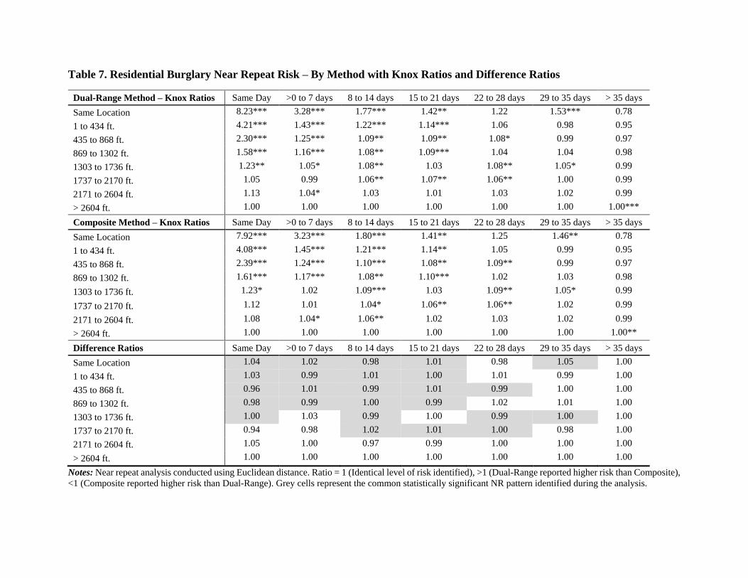
Table 7. Residential Burglary Near Repeat Risk – By Method with Knox Ratios and Difference Ratios
Dual-Range Method – Knox Ratios Same Day >0 to 7 days 8 to 14 days 15 to 21 days 22 to 28 days 29 to 35 days > 35 days
Same Location 8.23*** 3.28*** 1.77*** 1.42** 1.22 1.53*** 0.78
1 to 434 ft. 4.21*** 1.43*** 1.22*** 1.14*** 1.06 0.98 0.95
435 to 868 ft. 2.30*** 1.25*** 1.09** 1.09** 1.08* 0.99 0.97
869 to 1302 ft. 1.58*** 1.16*** 1.08** 1.09*** 1.04 1.04 0.98
1303 to 1736 ft. 1.23** 1.05* 1.08** 1.03 1.08** 1.05* 0.99
1737 to 2170 ft. 1.05 0.99 1.06** 1.07** 1.06** 1.00 0.99
2171 to 2604 ft. 1.13 1.04* 1.03 1.01 1.03 1.02 0.99
> 2604 ft. 1.00 1.00 1.00 1.00 1.00 1.00 1.00***
Composite Method – Knox Ratios Same Day >0 to 7 days 8 to 14 days 15 to 21 days 22 to 28 days 29 to 35 days > 35 days
Same Location 7.92*** 3.23*** 1.80*** 1.41** 1.25 1.46** 0.78
1 to 434 ft. 4.08*** 1.45*** 1.21*** 1.14** 1.05 0.99 0.95
435 to 868 ft. 2.39*** 1.24*** 1.10*** 1.08** 1.09** 0.99 0.97
869 to 1302 ft. 1.61*** 1.17*** 1.08** 1.10*** 1.02 1.03 0.98
1303 to 1736 ft. 1.23* 1.02 1.09*** 1.03 1.09** 1.05* 0.99
1737 to 2170 ft. 1.12 1.01 1.04* 1.06** 1.06** 1.02 0.99
2171 to 2604 ft. 1.08 1.04* 1.06** 1.02 1.03 1.02 0.99
> 2604 ft. 1.00 1.00 1.00 1.00 1.00 1.00 1.00**
Difference Ratios Same Day >0 to 7 days 8 to 14 days 15 to 21 days 22 to 28 days 29 to 35 days > 35 days
Same Location 1.04 1.02 0.98 1.01 0.98 1.05 1.00
1 to 434 ft. 1.03 0.99 1.01 1.00 1.01 0.99 1.00
435 to 868 ft. 0.96 1.01 0.99 1.01 0.99 1.00 1.00
869 to 1302 ft. 0.98 0.99 1.00 0.99 1.02 1.01 1.00
1303 to 1736 ft. 1.00 1.03 0.99 1.00 0.99 1.00 1.00
1737 to 2170 ft. 0.94 0.98 1.02 1.01 1.00 0.98 1.00
2171 to 2604 ft. 1.05 1.00 0.97 0.99 1.00 1.00 1.00
> 2604 ft. 1.00 1.00 1.00 1.00 1.00 1.00 1.00
Notes: Near repeat analysis conducted using Euclidean distance. Ratio = 1 (Identical level of risk identified), >1 (Dual-Range reported higher risk than Composite),
<1 (Composite reported higher risk than Dual-Range). Grey cells represent the common statistically significant NR pattern identified during the analysis.
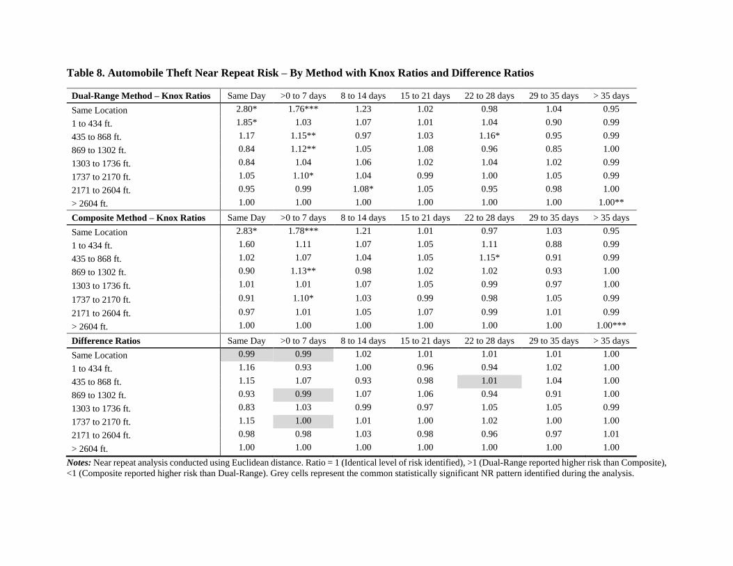
Table 8. Automobile Theft Near Repeat Risk – By Method with Knox Ratios and Difference Ratios
Dual-Range Method – Knox Ratios Same Day >0 to 7 days 8 to 14 days 15 to 21 days 22 to 28 days 29 to 35 days > 35 days
Same Location 2.80* 1.76*** 1.23 1.02 0.98 1.04 0.95
1 to 434 ft. 1.85* 1.03 1.07 1.01 1.04 0.90 0.99
435 to 868 ft. 1.17 1.15** 0.97 1.03 1.16* 0.95 0.99
869 to 1302 ft. 0.84 1.12** 1.05 1.08 0.96 0.85 1.00
1303 to 1736 ft. 0.84 1.04 1.06 1.02 1.04 1.02 0.99
1737 to 2170 ft. 1.05 1.10* 1.04 0.99 1.00 1.05 0.99
2171 to 2604 ft. 0.95 0.99 1.08* 1.05 0.95 0.98 1.00
> 2604 ft. 1.00 1.00 1.00 1.00 1.00 1.00 1.00**
Composite Method – Knox Ratios Same Day >0 to 7 days 8 to 14 days 15 to 21 days 22 to 28 days 29 to 35 days > 35 days
Same Location 2.83* 1.78*** 1.21 1.01 0.97 1.03 0.95
1 to 434 ft. 1.60 1.11 1.07 1.05 1.11 0.88 0.99
435 to 868 ft. 1.02 1.07 1.04 1.05 1.15* 0.91 0.99
869 to 1302 ft. 0.90 1.13** 0.98 1.02 1.02 0.93 1.00
1303 to 1736 ft. 1.01 1.01 1.07 1.05 0.99 0.97 1.00
1737 to 2170 ft. 0.91 1.10* 1.03 0.99 0.98 1.05 0.99
2171 to 2604 ft. 0.97 1.01 1.05 1.07 0.99 1.01 0.99
> 2604 ft. 1.00 1.00 1.00 1.00 1.00 1.00 1.00***
Difference Ratios Same Day >0 to 7 days 8 to 14 days 15 to 21 days 22 to 28 days 29 to 35 days > 35 days
Same Location 0.99 0.99 1.02 1.01 1.01 1.01 1.00
1 to 434 ft. 1.16 0.93 1.00 0.96 0.94 1.02 1.00
435 to 868 ft. 1.15 1.07 0.93 0.98 1.01 1.04 1.00
869 to 1302 ft. 0.93 0.99 1.07 1.06 0.94 0.91 1.00
1303 to 1736 ft. 0.83 1.03 0.99 0.97 1.05 1.05 0.99
1737 to 2170 ft. 1.15 1.00 1.01 1.00 1.02 1.00 1.00
2171 to 2604 ft. 0.98 0.98 1.03 0.98 0.96 0.97 1.01
> 2604 ft. 1.00 1.00 1.00 1.00 1.00 1.00 1.00
Notes: Near repeat analysis conducted using Euclidean distance. Ratio = 1 (Identical level of risk identified), >1 (Dual-Range reported higher risk than Composite),
<1 (Composite reported higher risk than Dual-Range). Grey cells represent the common statistically significant NR pattern identified during the analysis.
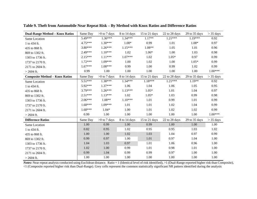
Table 9. Theft from Automobile Near Repeat Risk – By Method with Knox Ratios and Difference Ratios
Dual-Range Method – Knox Ratios Same Day >0 to 7 days 8 to 14 days 15 to 21 days 22 to 28 days 29 to 35 days > 35 days
Same Location 5.49*** 1.36*** 1.34*** 1.17** 1.21*** 1.19*** 0.92
1 to 434 ft. 4.75*** 1.30*** 1.08* 0.99 1.01 1.08* 0.97
435 to 868 ft. 3.80*** 1.26*** 1.15*** 1.08** 1.05 1.01 0.96
869 to 1302 ft. 2.49*** 1.10*** 1.02 1.06* 1.00 1.03 0.98
1303 to 1736 ft. 2.15*** 1.11*** 1.07*** 1.02 1.05* 0.97 0.99
1737 to 2170 ft. 1.72*** 1.09*** 1.00 1.02 1.00 1.05* 0.99
2171 to 2604 ft. 1.67*** 1.08*** 0.99 1.00 0.99 1.02 0.99
> 2604 ft. 0.99 1.00 1.00 1.00 1.00 1.00 1.00***
Composite Method – Knox Ratios Same Day >0 to 7 days 8 to 14 days 15 to 21 days 22 to 28 days 29 to 35 days > 35 days
Same Location 5.51*** 1.38*** 1.34*** 1.18*** 1.21*** 1.19** 0.92
1 to 434 ft. 5.92*** 1.37*** 1.06 1.04 1.06 1.05 0.95
435 to 868 ft. 3.79*** 1.26*** 1.13*** 1.05* 1.01 1.04 0.97
869 to 1302 ft. 2.51*** 1.13*** 1.02 1.05* 1.03 0.99 0.98
1303 to 1736 ft. 2.06*** 1.08** 1.10*** 1.01 0.99 1.01 0.99
1737 to 2170 ft. 1.68*** 1.09*** 1.01 1.01 1.02 1.04 0.99
2171 to 2604 ft. 1.68*** 1.04* 1.00 1.01 1.02 1.02 0.99
> 2604 ft. 0.99 1.00 1.00 1.00 1.00 1.00 1.00***
Difference Ratios Same Day >0 to 7 days 8 to 14 days 15 to 21 days 22 to 28 days 29 to 35 days > 35 days
Same Location 1.00 0.99 1.00 0.99 1.00 1.00 1.00
1 to 434 ft. 0.82 0.95 1.02 0.95 0.95 1.03 1.02
435 to 868 ft. 1.00 1.00 1.02 1.03 1.04 0.97 0.99
869 to 1302 ft. 0.99 0.97 1.00 1.01 0.97 1.04 1.00
1303 to 1736 ft. 1.04 1.03 0.97 1.01 1.06 0.96 1.00
1737 to 2170 ft. 1.02 1.00 0.99 1.01 0.98 1.01 1.00
2171 to 2604 ft. 0.99 1.04 0.99 0.99 0.97 1.00 1.00
> 2604 ft. 1.00 1.00 1.00 1.00 1.00 1.00 1.00
Notes: Near repeat analysis conducted using Euclidean distance. Ratio = 1 (Identical level of risk identified), >1 (Dual-Range reported higher risk than Composite),
<1 (Composite reported higher risk than Dual-Range). Grey cells represent the common statistically significant NR pattern identified during the analysis