upper-mantle flow beneath french polynesia from shear wave
TRANSCRIPT
HAL Id: hal-01249275https://hal.archives-ouvertes.fr/hal-01249275
Submitted on 31 Dec 2015
HAL is a multi-disciplinary open accessarchive for the deposit and dissemination of sci-entific research documents, whether they are pub-lished or not. The documents may come fromteaching and research institutions in France orabroad, or from public or private research centers.
L’archive ouverte pluridisciplinaire HAL, estdestinée au dépôt et à la diffusion de documentsscientifiques de niveau recherche, publiés ou non,émanant des établissements d’enseignement et derecherche français ou étrangers, des laboratoirespublics ou privés.
Upper-mantle flow beneath French Polynesia from shearwave splitting
Fabrice R. Fontaine, Guilhem Barruol, Andrea Tommasi, Götz H.R.Bokelmann
To cite this version:Fabrice R. Fontaine, Guilhem Barruol, Andrea Tommasi, Götz H.R. Bokelmann. Upper-mantle flowbeneath French Polynesia from shear wave splitting. Geophysical Journal International, Oxford Uni-versity Press (OUP), 2007, 170, �10.1111/j.1365-246X.2007.03475.x�. �hal-01249275�

June 2, 2007 15:5 Geophysical Journal International gji˙3475
Geophys. J. Int. (2007) doi: 10.1111/j.1365-246X.2007.03475.x
GJI
Sei
smol
ogy
Upper-mantle flow beneath French Polynesia from shearwave splitting
Fabrice R. Fontaine,1,2 Guilhem Barruol,1,3 Andrea Tommasi3
and Gotz H. R. Bokelmann3
1Laboratoire Terre-Ocean, Universite de Polynesie francaise, BP 6570, 98702 Faaa, Tahiti, Polynesie francaise2Research School of Earth Sciences, Australian National University, Building 61, Mills Road, Canberra, ACT 0200, Australia.E-mail: [email protected] Montpellier, CNRS, Universite Montpellier II, F-34095 Montpellier Cedex 5, France
Accepted 2007 April 23. Received 2007 April 23; in original form 2006 July 16
S U M M A R YUpper-mantle flow beneath the South Pacific is investigated by analysing shear wave splittingparameters at eight permanent long-period and broad-band seismic stations and 10 broad-bandstations deployed in French Polynesia from 2001 to 2005 in the framework of the PolynesianLithosphere and Upper Mantle Experiment (PLUME). Despite the small number of eventsand the rather poor backazimuthal coverage due to the geographical distribution of the naturalseismicity, upper-mantle seismic anisotropy has been detected at all stations except at Tahitiwhere two permanent stations with 15 yr of data show an apparent isotropy. The medianvalue of fast polarization azimuths (N67.5◦W) is parallel to the present Pacific absolute platemotion direction in French Polynesia (APM: N67◦W). This suggests that the observed SKSfast polarization directions result mainly from olivine crystal preferred orientations producedby deformation in the sublithospheric mantle due to viscous entrainment by the moving PacificPlate and preserved in the lithosphere as the plate cools. However, analysis of individualmeasurements highlights variations of splitting parameters with event backazimuth that implyan actual upper-mantle structure more complex than a single anisotropic layer with horizontalfast axis. A forward approach shows that a two-layer structure of anisotropy beneath FrenchPolynesia better explains the splitting observations than a single anisotropic layer. Second-order variations in the measurements may also indicate the presence of small-scale lateralheterogeneities. The influence of plumes or fracture zones within the studied area does notappear to dominate the large-scale anisotropy pattern but may explain these second-ordersplitting variations across the network.
Key words: French polynesia, seismic anisotropy, shear wave splitting, upper mantle.
1 I N T RO D U C T I O N
The Pacific Plate, which is almost entirely of oceanic origin, is oneof the largest and fastest-moving plates of our planet. The structureof oceanic lithosphere should in principle be controlled by the inter-play between cooling and thickening and the deformation inducedat the base of the lithosphere by the motion of the plate relative tothe deeper mantle (Schubert et al. 1976; Tommasi 1998). However,the small-scale structure of the upper mantle beneath the Pacific isnot yet well known, due to the difficulty in deploying geophysicalinstruments in remote oceanic environments. In particular, there isa lack of permanent seismic stations providing the necessary obser-vations to determine accurate upper-mantle tomographic images, tomap the mantle flow, or to measure the depth of the major discon-tinuities. Global and regional surface wave tomographic models(e.g. Nishimura & Forsyth 1989; Montagner & Tanimoto 1991;
Ekstrom & Dziewonski 1998; Montagner 2002; Maggi et al.2006a,b), body wave global tomographic models (e.g. Grand et al.1997; van der Hilst et al. 1997; Montelli et al. 2004) and bathymetricdata (Smith & Sandwell 1994; Jordahl et al. 2004) have indeed ratherpoor resolution in the South Pacific. Although information on man-tle plumes location has been derived from the analysis of volcanicstructures and lineaments (e.g. Duncan & Richards 1991; Clouard &Bonneville 2005), the depth origin of these plumes and their effecton the overlying lithosphere are also still debated.
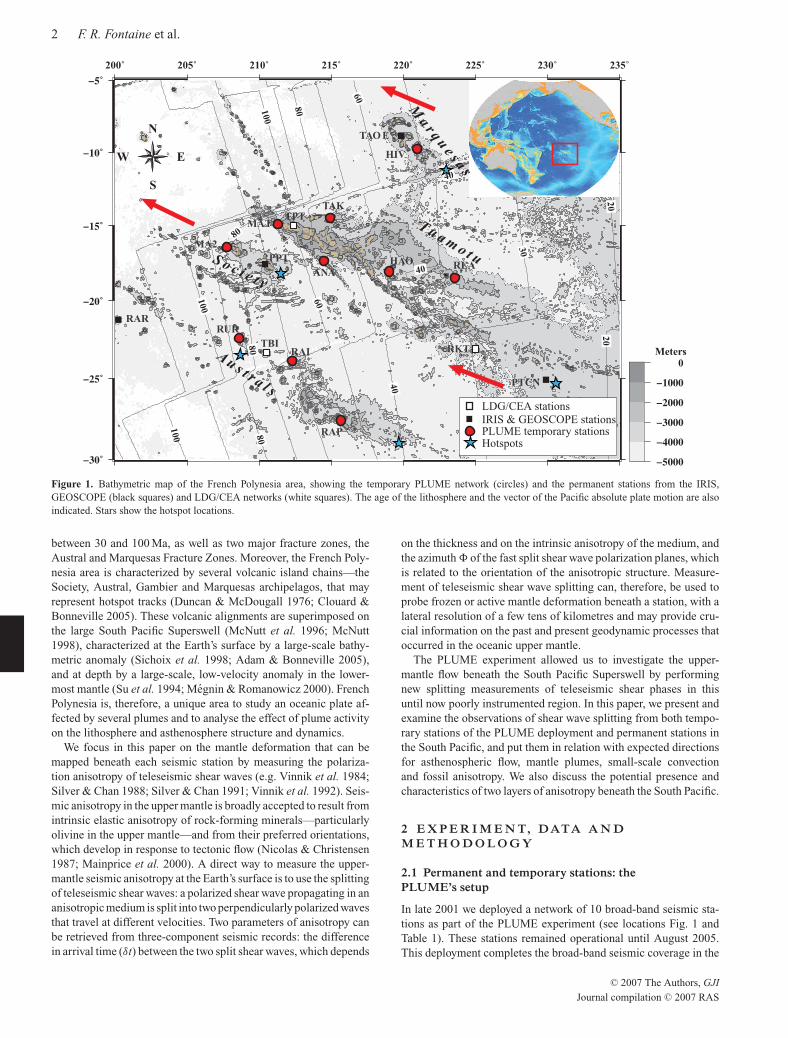
In order to constrain the structure of the South Pacific uppermantle, we deployed a temporary network of 10 broad-band three-component seismic stations on French Polynesia Islands (Fig. 1) inthe frame of the Polynesian Lithosphere and Upper Mantle Exper-iment (PLUME) (Barruol et al. 2002). This South Pacific region isof particular interest since it lies far from any plate boundary, andit is large enough to sample oceanic lithosphere with ages varying
C© 2007 The Authors 1Journal compilation C© 2007 RAS
June 2, 2007 15:5 Geophysical Journal International gji˙3475
2 F. R. Fontaine et al.
200˚ 205˚ 210˚ 215˚ 220˚ 225˚ 230˚ 235˚
0Meters
2020
40
40
40
60
60
80
80
80
80
30
40
100
100
100
ANAHAO
HIV
MA2
MAT
RAI
RAP
REA
RURRAR
TAK
RKTTBI
TPT
PPT
PTCN
TAO E
LDG/CEA stationsIRIS & GEOSCOPE stationsPLUME temporary stationsHotspots
Ma rq u
e s a s
Tu a m o t u
Au s t r a l s
S o c i e t y
S
E
N
W
Figure 1. Bathymetric map of the French Polynesia area, showing the temporary PLUME network (circles) and the permanent stations from the IRIS,GEOSCOPE (black squares) and LDG/CEA networks (white squares). The age of the lithosphere and the vector of the Pacific absolute plate motion are alsoindicated. Stars show the hotspot locations.
between 30 and 100 Ma, as well as two major fracture zones, theAustral and Marquesas Fracture Zones. Moreover, the French Poly-nesia area is characterized by several volcanic island chains—theSociety, Austral, Gambier and Marquesas archipelagos, that mayrepresent hotspot tracks (Duncan & McDougall 1976; Clouard &Bonneville 2005). These volcanic alignments are superimposed onthe large South Pacific Superswell (McNutt et al. 1996; McNutt1998), characterized at the Earth’s surface by a large-scale bathy-metric anomaly (Sichoix et al. 1998; Adam & Bonneville 2005),and at depth by a large-scale, low-velocity anomaly in the lower-most mantle (Su et al. 1994; Megnin & Romanowicz 2000). FrenchPolynesia is, therefore, a unique area to study an oceanic plate af-fected by several plumes and to analyse the effect of plume activityon the lithosphere and asthenosphere structure and dynamics.
We focus in this paper on the mantle deformation that can bemapped beneath each seismic station by measuring the polariza-tion anisotropy of teleseismic shear waves (e.g. Vinnik et al. 1984;Silver & Chan 1988; Silver & Chan 1991; Vinnik et al. 1992). Seis-mic anisotropy in the upper mantle is broadly accepted to result fromintrinsic elastic anisotropy of rock-forming minerals—particularlyolivine in the upper mantle—and from their preferred orientations,which develop in response to tectonic flow (Nicolas & Christensen1987; Mainprice et al. 2000). A direct way to measure the upper-mantle seismic anisotropy at the Earth’s surface is to use the splittingof teleseismic shear waves: a polarized shear wave propagating in ananisotropic medium is split into two perpendicularly polarized wavesthat travel at different velocities. Two parameters of anisotropy canbe retrieved from three-component seismic records: the differencein arrival time (δt) between the two split shear waves, which depends
on the thickness and on the intrinsic anisotropy of the medium, andthe azimuth � of the fast split shear wave polarization planes, whichis related to the orientation of the anisotropic structure. Measure-ment of teleseismic shear wave splitting can, therefore, be used toprobe frozen or active mantle deformation beneath a station, with alateral resolution of a few tens of kilometres and may provide cru-cial information on the past and present geodynamic processes thatoccurred in the oceanic upper mantle.
The PLUME experiment allowed us to investigate the upper-mantle flow beneath the South Pacific Superswell by performingnew splitting measurements of teleseismic shear phases in thisuntil now poorly instrumented region. In this paper, we present andexamine the observations of shear wave splitting from both tempo-rary stations of the PLUME deployment and permanent stations inthe South Pacific, and put them in relation with expected directionsfor asthenospheric flow, mantle plumes, small-scale convectionand fossil anisotropy. We also discuss the potential presence andcharacteristics of two layers of anisotropy beneath the South Pacific.
2 E X P E R I M E N T, DATA A N DM E T H O D O L O G Y
2.1 Permanent and temporary stations: thePLUME’s setup
In late 2001 we deployed a network of 10 broad-band seismic sta-tions as part of the PLUME experiment (see locations Fig. 1 andTable 1). These stations remained operational until August 2005.This deployment completes the broad-band seismic coverage in the
C© 2007 The Authors, GJI
Journal compilation C© 2007 RAS
June 2, 2007 15:5 Geophysical Journal International gji˙3475
Shear wave splitting beneath French Polynesia 3
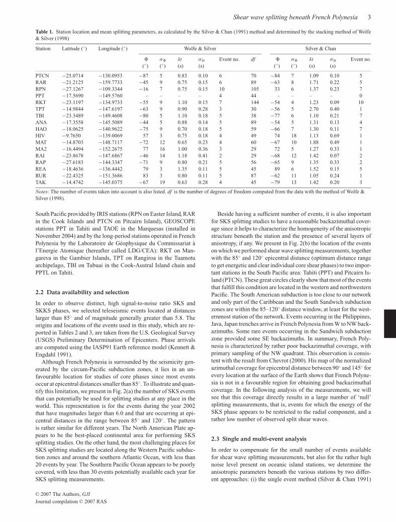
Table 1. Station location and mean splitting parameters, as calculated by the Silver & Chan (1991) method and determined by the stacking method of Wolfe& Silver (1998)
Station Latitude (◦) Longitude (◦) Wolfe & Silver Silver & Chan
� σ� δt σδt Event no. df � σ� δt σδt Event no.(◦) (◦) (s) (s) (◦) (◦) (s) (s)
PTCN −25.0714 −130.0953 −87 5 0.83 0.10 6 70 −84 7 1.09 0.10 5RAR −21.2125 −159.7733 −45 9 0.75 0.15 6 89 −63 8 1.71 0.22 5RPN −27.1267 −109.3344 −16 7 0.75 0.15 10 105 33 6 1.37 0.23 7PPT −17.5690 −149.5760 – – – – 4 44 – – – – 0RKT −23.1197 −134.9733 −55 9 1.10 0.15 7 144 −54 4 1.23 0.09 10TPT −14.9844 −147.6197 −63 9 0.90 0.28 3 30 −56 5 2.70 0.40 1TBI −23.3489 −149.4608 −80 5 1.10 0.18 5 38 −77 6 1.10 0.21 7ANA −17.3558 −145.5089 −44 5 0.88 0.14 5 89 −54 5 1.31 0.13 4HAO −18.0625 −140.9622 −75 9 0.70 0.18 5 59 −66 7 1.30 0.11 7HIV −9.7650 −139.0069 57 3 0.75 0.18 4 49 74 18 1.13 0.69 1MAT −14.8703 −148.7117 −72 12 0.65 0.23 4 60 −67 10 1.88 0.49 1MA2 −16.4494 −152.2675 77 16 1.00 0.36 3 29 72 5 1.27 0.33 1RAI −23.8678 −147.6867 −46 14 1.18 0.41 2 29 −68 12 1.42 0.07 2RAP −27.6183 −144.3347 −71 9 0.80 0.21 5 56 −65 9 1.35 0.33 2REA −18.4636 −136.4442 79 3 1.35 0.11 5 45 89 6 1.52 0.15 5RUR −22.4325 −151.3686 83 3 0.80 0.11 5 87 −62 11 1.05 0.24 1TAK −14.4742 −145.0375 −67 19 0.63 0.28 4 45 −79 13 1.42 0.20 3
Notes: The number of events taken into account is also listed. df is the number of degrees of freedom computed from the data with the method of Wolfe &Silver (1998).
South Pacific provided by IRIS stations (RPN on Easter Island, RARin the Cook Islands and PTCN on Pitcairn Island), GEOSCOPEstations PPT in Tahiti and TAOE in the Marquesas (installed inNovember 2004) and by the long-period stations operated in FrenchPolynesia by the Laboratoire de Geophysique du Commissariat al’Energie Atomique (hereafter called LDG/CEA): RKT on Man-gareva in the Gambier Islands, TPT on Rangiroa in the Tuamotuarchipelago, TBI on Tubuai in the Cook-Austral Island chain andPPTL on Tahiti.
2.2 Data availability and selection
In order to observe distinct, high signal-to-noise ratio SKS andSKKS phases, we selected teleseismic events located at distanceslarger than 85◦ and of magnitude generally greater than 5.8. Theorigins and locations of the events used in this study, which are re-ported in Tables 2 and 3, are taken from the U.S. Geological Survey(USGS) Preliminary Determination of Epicenters. Phase arrivalsare computed using the IASP91 Earth reference model (Kennett &Engdahl 1991).
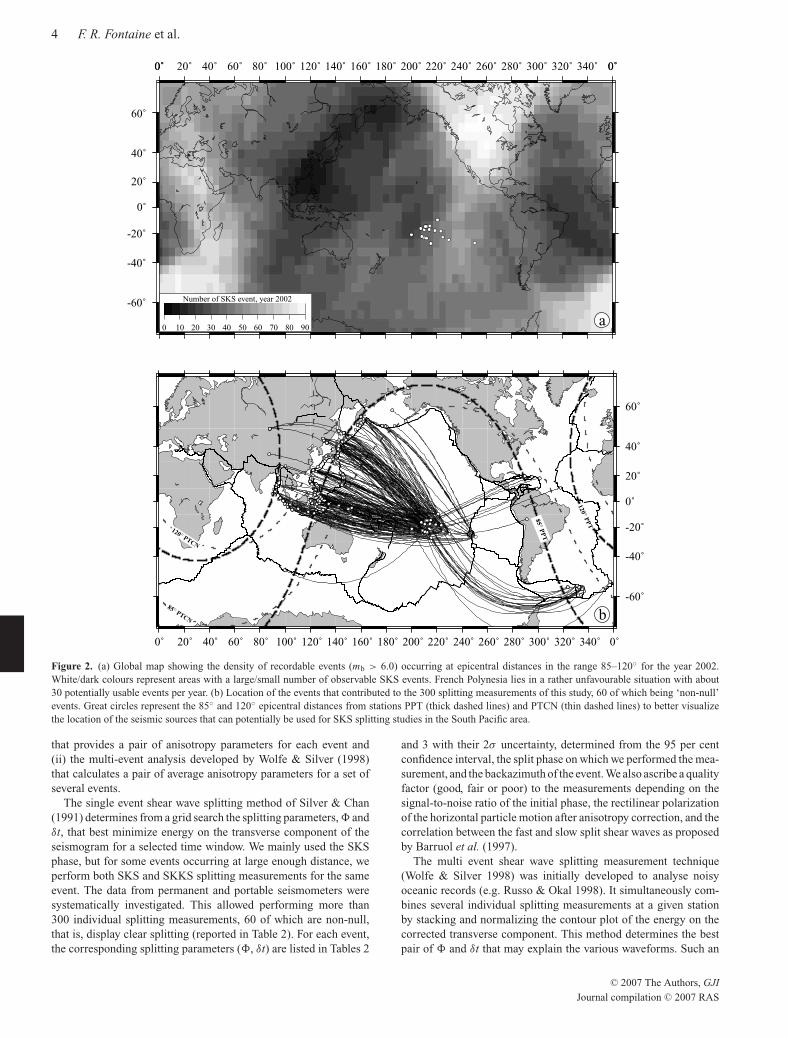
Although French Polynesia is surrounded by the seismicity gen-erated by the circum-Pacific subduction zones, it lies in an un-favourable location for studies of core phases since most eventsoccur at epicentral distances smaller than 85◦. To illustrate and quan-tify this limitation, we present in Fig. 2(a) the number of SKS eventsthat can potentially be used for splitting studies at any place in theworld. This representation is for the events during the year 2002that have magnitudes larger than 6.0 and that are occurring at epi-central distances in the range between 85◦ and 120◦. The patternis rather similar for different years. The North American Plate ap-pears to be the best-placed continental area for performing SKSsplitting studies. On the other hand, the most challenging places forSKS splitting studies are located along the Western Pacific subduc-tion zones and around the southern Atlantic Ocean, with less than20 events by year. The Southern Pacific Ocean appears to be poorlycovered, with less than 30 events potentially available each year forSKS splitting measurements.
Beside having a sufficient number of events, it is also importantfor SKS splitting studies to have a reasonable backazimuthal cover-age since it helps to characterize the homogeneity of the anisotropicstructure beneath the station and the presence of several layers ofanisotropy, if any. We present in Fig. 2(b) the location of the eventson which we performed shear wave splitting measurements, togetherwith the 85◦ and 120◦ epicentral distance (optimum distance rangeto get energetic and clear individual core shear phases) to two impor-tant stations in the South Pacific area: Tahiti (PPT) and Pitcairn Is-land (PTCN). These great circles clearly show that most of the eventsthat fulfill this condition are located in the western and northwesternPacific. The South American subduction is too close to our networkand only part of the Caribbean and the South Sandwich subductionzones are within the 85–120◦ distance window, at least for the west-ernmost station of the network. Events occurring in the Philippines,Java, Japan trenches arrive in French Polynesia from W to NW back-azimuths. Some rare events occurring in the Sandwich subductionzone provided some SE backazimuths. In summary, French Poly-nesia is characterized by rather poor backazimuthal coverage, withprimary sampling of the NW quadrant. This observation is consis-tent with the result from Chevrot (2000). His map of the normalizedazimuthal coverage for epicentral distance between 90◦ and 145◦ forevery location at the surface of the Earth shows that French Polyne-sia is not in a favourable region for obtaining good backazimuthalcoverage. In the following analysis of the measurements, we willsee that this coverage directly results in a large number of ‘null’splitting measurements, that is, events for which the energy of theSKS phase appears to be restricted to the radial component, and arather low number of observed split shear waves.
2.3 Single and multi-event analysis
In order to compensate for the small number of events availablefor shear wave splitting measurements, but also for the rather highnoise level present on oceanic island stations, we determine theanisotropic parameters beneath the various stations by two differ-ent approaches: (i) the single event method (Silver & Chan 1991)
C© 2007 The Authors, GJI
Journal compilation C© 2007 RAS
June 2, 2007 15:5 Geophysical Journal International gji˙3475
4 F. R. Fontaine et al.
0˚ 20˚ 40˚ 60˚ 80˚ 100˚ 120˚ 140˚ 160˚ 180˚ 200˚ 220˚ 240˚ 260˚ 280˚ 300˚ 320˚ 340˚ 0˚
0˚
20˚
40˚
60˚
85
20
-60˚
-40˚
-20˚
b
0˚ 20˚ 40˚ 60˚ 80˚ 100˚ 120˚ 140˚ 160˚ 180˚ 200˚ 220˚ 240˚ 260˚ 280˚ 300˚ 320˚ 340˚ 0˚
0˚
20˚
40˚
60˚
0˚ 0˚
-60˚
-40˚
-20˚
Number of SKS event, year 2002
0 10 20 30 40 50 60 70 80 90a
85° PP
T
120° PPT
85° PTCN
120° PTCN
Figure 2. (a) Global map showing the density of recordable events (mb > 6.0) occurring at epicentral distances in the range 85–120◦ for the year 2002.White/dark colours represent areas with a large/small number of observable SKS events. French Polynesia lies in a rather unfavourable situation with about30 potentially usable events per year. (b) Location of the events that contributed to the 300 splitting measurements of this study, 60 of which being ‘non-null’events. Great circles represent the 85◦ and 120◦ epicentral distances from stations PPT (thick dashed lines) and PTCN (thin dashed lines) to better visualizethe location of the seismic sources that can potentially be used for SKS splitting studies in the South Pacific area.
that provides a pair of anisotropy parameters for each event and(ii) the multi-event analysis developed by Wolfe & Silver (1998)that calculates a pair of average anisotropy parameters for a set ofseveral events.
The single event shear wave splitting method of Silver & Chan(1991) determines from a grid search the splitting parameters, � andδt, that best minimize energy on the transverse component of theseismogram for a selected time window. We mainly used the SKSphase, but for some events occurring at large enough distance, weperform both SKS and SKKS splitting measurements for the sameevent. The data from permanent and portable seismometers weresystematically investigated. This allowed performing more than300 individual splitting measurements, 60 of which are non-null,that is, display clear splitting (reported in Table 2). For each event,the corresponding splitting parameters (�, δt) are listed in Tables 2
and 3 with their 2σ uncertainty, determined from the 95 per centconfidence interval, the split phase on which we performed the mea-surement, and the backazimuth of the event. We also ascribe a qualityfactor (good, fair or poor) to the measurements depending on thesignal-to-noise ratio of the initial phase, the rectilinear polarizationof the horizontal particle motion after anisotropy correction, and thecorrelation between the fast and slow split shear waves as proposedby Barruol et al. (1997).
The multi event shear wave splitting measurement technique(Wolfe & Silver 1998) was initially developed to analyse noisyoceanic records (e.g. Russo & Okal 1998). It simultaneously com-bines several individual splitting measurements at a given stationby stacking and normalizing the contour plot of the energy on thecorrected transverse component. This method determines the bestpair of � and δt that may explain the various waveforms. Such an
C© 2007 The Authors, GJI
Journal compilation C© 2007 RAS
June 2, 2007 15:5 Geophysical Journal International gji˙3475
Shear wave splitting beneath French Polynesia 5
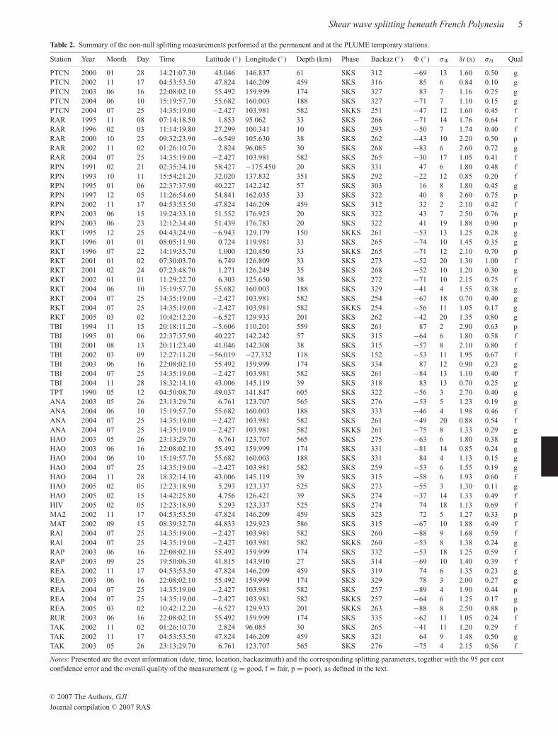
Table 2. Summary of the non-null splitting measurements performed at the permanent and at the PLUME temporary stations.
Station Year Month Day Time Latitude (◦) Longitude (◦) Depth (km) Phase Backaz (◦) � (◦) σ� δt (s) σδt Qual
PTCN 2000 01 28 14:21:07.30 43.046 146.837 61 SKS 312 −69 13 1.60 0.50 gPTCN 2002 11 17 04:53:53.50 47.824 146.209 459 SKS 316 85 6 0.84 0.10 gPTCN 2003 06 16 22:08:02.10 55.492 159.999 174 SKS 327 83 7 1.16 0.25 gPTCN 2004 06 10 15:19:57.70 55.682 160.003 188 SKS 327 −71 7 1.10 0.15 gPTCN 2004 07 25 14:35:19.00 −2.427 103.981 582 SKKS 251 −47 12 1.60 0.45 fRAR 1995 11 08 07:14:18.50 1.853 95.062 33 SKS 266 −71 14 1.76 0.64 fRAR 1996 02 03 11:14:19.80 27.299 100.341 10 SKS 293 −50 7 1.74 0.40 fRAR 2000 10 25 09:32:23.90 −6.549 105.630 38 SKS 262 −43 10 2.20 0.50 pRAR 2002 11 02 01:26:10.70 2.824 96.085 30 SKS 268 −83 6 2.60 0.72 gRAR 2004 07 25 14:35:19.00 −2.427 103.981 582 SKS 265 −30 17 1.05 0.41 fRPN 1991 02 21 02:35:34.10 58.427 −175.450 20 SKS 331 47 6 1.80 0.48 fRPN 1993 10 11 15:54:21.20 32.020 137.832 351 SKS 292 −22 12 0.85 0.20 fRPN 1995 01 06 22:37:37.90 40.227 142.242 57 SKS 303 16 8 1.80 0.45 gRPN 1997 12 05 11:26:54.60 54.841 162.035 33 SKS 322 40 8 2.60 0.75 pRPN 2002 11 17 04:53:53.50 47.824 146.209 459 SKS 312 32 2 2.10 0.42 fRPN 2003 06 15 19:24:33.10 51.552 176.923 20 SKS 322 43 7 2.50 0.76 pRPN 2003 06 23 12:12:34.40 51.439 176.783 20 SKS 322 41 19 1.88 0.90 pRKT 1995 12 25 04:43:24.90 −6.943 129.179 150 SKKS 261 −53 13 1.25 0.28 gRKT 1996 01 01 08:05:11.90 0.724 119.981 33 SKS 265 −74 10 1.45 0.35 gRKT 1996 07 22 14:19:35.70 1.000 120.450 33 SKKS 265 −71 12 2.10 0.70 pRKT 2001 01 02 07:30:03.70 6.749 126.809 33 SKS 273 −52 20 1.30 1.00 fRKT 2001 02 24 07:23:48.70 1.271 126.249 35 SKS 268 −52 10 1.20 0.30 gRKT 2002 01 01 11:29:22.70 6.303 125.650 38 SKS 272 −71 10 2.15 0.75 fRKT 2004 06 10 15:19:57.70 55.682 160.003 188 SKS 329 −41 4 1.55 0.38 gRKT 2004 07 25 14:35:19.00 −2.427 103.981 582 SKS 254 −67 18 0.70 0.40 gRKT 2004 07 25 14:35:19.00 −2.427 103.981 582 SKKS 254 −56 11 1.05 0.17 gRKT 2005 03 02 10:42:12.20 −6.527 129.933 201 SKS 262 −42 20 1.35 0.80 gTBI 1994 11 15 20:18:11.20 −5.606 110.201 559 SKS 261 87 2 2.90 0.63 pTBI 1995 01 06 22:37:37.90 40.227 142.242 57 SKS 315 −64 6 1.80 0.58 fTBI 2001 08 13 20:11:23.40 41.046 142.308 38 SKS 315 −57 8 2.10 0.80 fTBI 2002 03 09 12:27:11.20 −56.019 −27.332 118 SKS 152 −53 11 1.95 0.67 fTBI 2003 06 16 22:08:02.10 55.492 159.999 174 SKS 334 87 12 0.90 0.23 gTBI 2004 07 25 14:35:19.00 −2.427 103.981 582 SKS 261 −84 13 1.10 0.40 fTBI 2004 11 28 18:32:14.10 43.006 145.119 39 SKS 318 83 13 0.70 0.25 gTPT 1990 05 12 04:50:08.70 49.037 141.847 605 SKS 322 −56 3 2.70 0.40 gANA 2003 05 26 23:13:29.70 6.761 123.707 565 SKS 276 −53 5 1.23 0.19 gANA 2004 06 10 15:19:57.70 55.682 160.003 188 SKS 333 −46 4 1.98 0.46 fANA 2004 07 25 14:35:19.00 −2.427 103.981 582 SKS 261 −49 20 0.88 0.54 fANA 2004 07 25 14:35:19.00 −2.427 103.981 582 SKKS 261 −75 8 1.33 0.29 gHAO 2003 05 26 23:13:29.70 6.761 123.707 565 SKS 275 −63 6 1.80 0.38 gHAO 2003 06 16 22:08:02.10 55.492 159.999 174 SKS 331 −81 14 0.85 0.24 gHAO 2004 06 10 15:19:57.70 55.682 160.003 188 SKS 331 84 4 1.13 0.15 gHAO 2004 07 25 14:35:19.00 −2.427 103.981 582 SKS 259 −53 6 1.55 0.19 gHAO 2004 11 28 18:32:14.10 43.006 145.119 39 SKS 315 −58 6 1.93 0.60 fHAO 2005 02 05 12:23:18.90 5.293 123.337 525 SKS 273 −55 3 1.30 0.11 gHAO 2005 02 15 14:42:25.80 4.756 126.421 39 SKS 274 −37 14 1.33 0.49 fHIV 2005 02 05 12:23:18.90 5.293 123.337 525 SKS 274 74 18 1.13 0.69 fMA2 2002 11 17 04:53:53.50 47.824 146.209 459 SKS 323 72 5 1.27 0.33 pMAT 2002 09 15 08:39:32.70 44.833 129.923 586 SKS 315 −67 10 1.88 0.49 fRAI 2004 07 25 14:35:19.00 −2.427 103.981 582 SKS 260 −88 9 1.68 0.59 fRAI 2004 07 25 14:35:19.00 −2.427 103.981 582 SKKS 260 −53 8 1.38 0.24 gRAP 2003 06 16 22:08:02.10 55.492 159.999 174 SKS 332 −53 18 1.25 0.59 fRAP 2003 09 25 19:50:06.30 41.815 143.910 27 SKS 314 −69 10 1.40 0.39 fREA 2002 11 17 04:53:53.50 47.824 146.209 459 SKS 319 74 6 1.35 0.23 gREA 2003 06 16 22:08:02.10 55.492 159.999 174 SKS 329 78 3 2.00 0.27 gREA 2004 07 25 14:35:19.00 −2.427 103.981 582 SKS 257 −89 4 1.90 0.44 pREA 2004 07 25 14:35:19.00 −2.427 103.981 582 SKKS 257 −64 6 1.25 0.17 gREA 2005 03 02 10:42:12.20 −6.527 129.933 201 SKKS 263 −88 8 2.50 0.88 pRUR 2003 06 16 22:08:02.10 55.492 159.999 174 SKS 335 −62 11 1.05 0.24 fTAK 2002 11 02 01:26:10.70 2.824 96.085 30 SKS 265 −41 11 1.20 0.29 fTAK 2002 11 17 04:53:53.50 47.824 146.209 459 SKS 321 64 9 1.48 0.50 gTAK 2003 05 26 23:13:29.70 6.761 123.707 565 SKS 276 −75 4 2.15 0.56 f
Notes: Presented are the event information (date, time, location, backazimuth) and the corresponding splitting parameters, together with the 95 per centconfidence error and the overall quality of the measurement (g = good, f = fair, p = poor), as defined in the text.
C© 2007 The Authors, GJI
Journal compilation C© 2007 RAS
June 2, 2007 15:5 Geophysical Journal International gji˙3475
6 F. R. Fontaine et al.
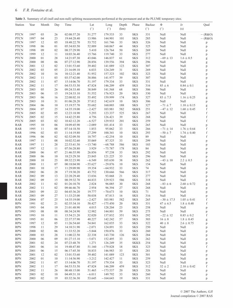
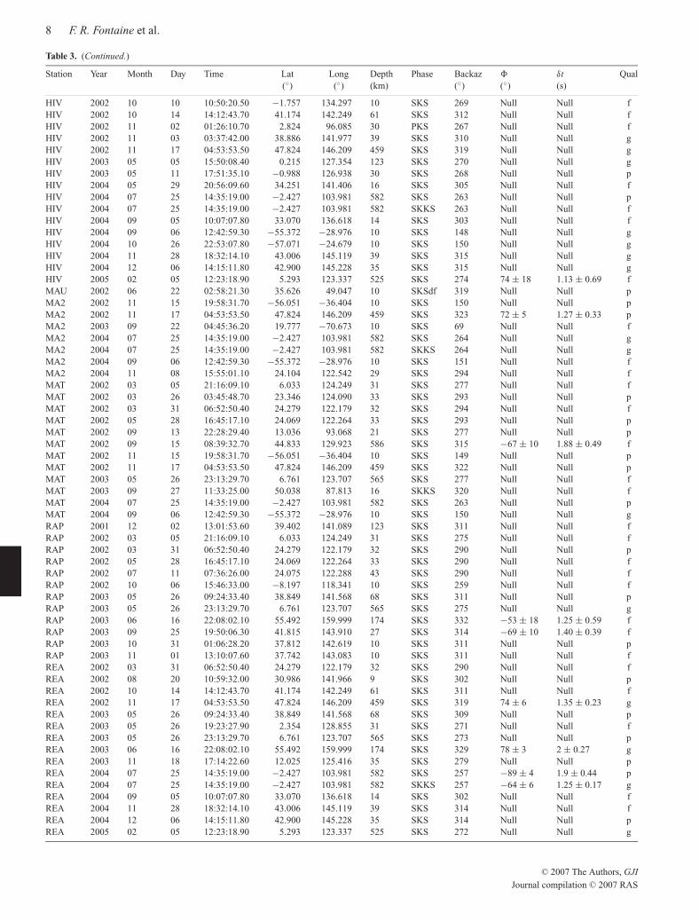
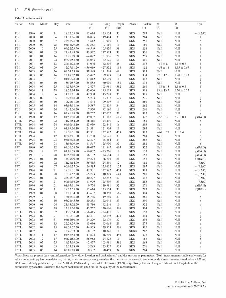
Table 3. Summary of all (null and non-null) splitting measurements performed at the permanent and at the PLUME temporary sites.
Station Year Month Day Time Lat Long Depth Phase Backaz � δt Qual(◦) (◦) (km) (◦) (◦) (s)
PTCN 1997 03 26 02:08:57.20 51.277 179.533 33 SKS 331 Null Null − (R&O)PTCN 1997 04 23 19:44:28.40 13.986 144.901 101 SKS 285 Null Null − (R&O)PTCN 1997 12 05 18:48:22.70 53.752 161.746 33 SKS 326 Null Null pPTCN 1998 06 01 05:34:03.50 52.889 160.067 44 SKS 325 Null Null pPTCN 1998 09 02 08:37:29.90 5.410 126.764 50 SKS 269 Null Null pPTCN 1999 12 11 18:03:36.40 15.766 119.740 33 SKS 277 Null Null pPTCN 2000 01 28 14:21:07.30 43.046 146.837 61 SKS 312 −69 ± 13 1.6 ± 0.5 gPTCN 2000 08 06 07:27:12.90 28.856 139.556 394 SKS 296 Null Null gPTCN 2001 12 02 13:01:53.60 39.402 141.089 123 SKS 307 Null Null pPTCN 2002 03 05 21:16:09.10 6.033 124.249 31 SKS 269 Null Null pPTCN 2002 10 16 10:12:21.40 51.952 157.323 102 SKS 323 Null Null pPTCN 2002 11 03 03:37:42.00 38.886 141.977 39 SKS 307 Null Null pPTCN 2002 11 07 15:14:06.70 51.197 179.334 33 SKS 331 Null Null pPTCN 2002 11 17 04:53:53.50 47.824 146.209 459 SKS 316 85 ± 6 0.84 ± 0.1 gPTCN 2003 05 26 09:24:33.40 38.849 141.568 68 SKS 306 Null Null pPTCN 2003 06 15 19:24:33.10 51.552 176.923 20 SKS 330 Null Null pPTCN 2003 06 16 22:08:02.10 55.492 159.999 174 SKS 327 83 ± 7.5 1.16 ± 0.25 gPTCN 2003 10 31 01:06:28.20 37.812 142.619 10 SKS 306 Null Null pPTCN 2004 06 10 15:19:57.70 55.682 160.003 188 SKS 327 −71 ± 7 1.10 ± 0.15 gPTCN 2004 07 25 14:35:19.00 −2.427 103.981 582 SKKS 251 −47 ± 12 1.60 ± 0.45 fPTCN 2005 02 05 12:23:18.90 5.293 123.337 525 SKS 267 Null Null fPTCN 2005 02 15 14:42:25.80 4.756 126.421 39 SKS 268 Null Null fPTCN 2005 03 02 10:42:12.20 −6.527 129.933 201 SKS 259 Null Null fRAR 1995 10 06 18:09:45.90 −2.089 101.414 33 SKS 265 Null Null pRAR 1995 11 08 07:14:18.50 1.853 95.062 33 SKS 266 −71 ± 14 1.76 ± 0.64 fRAR 1996 02 03 11:14:19.80 27.299 100.341 10 SKS 293 −50 ± 7 1.74 ± 0.40 fRAR 1996 06 02 02:52:09.50 10.797 −42.254 10 SKS 89 Null Null fRAR 1997 11 08 10:02:52.60 35.069 87.325 33 SKS 299 Null Null pRAR 1997 11 28 22:53:41.50 −13.740 −68.788 586 SKS 103 Null Null pRAR 1997 12 11 07:56:28.80 3.929 −75.787 178 SKS 84 Null Null pRAR 2000 06 07 21:46:55.90 26.856 97.238 33 SKS 292 Null Null pRAR 2000 06 10 18:23:29.30 23.843 121.225 33 SKS 296 Null Null pRAR 2000 10 25 09:32:23.90 −6.549 105.630 38 SKS 262 −43 ± 10 2.2 ± 0.5 pRAR 2000 11 07 00:18:04.90 −55.627 −29.876 10 SKS 154 Null Null pRAR 2001 10 17 11:29:09.90 19.354 −64.932 33 SKS 74 Null Null pRAR 2002 06 28 17:19:30.20 43.752 130.666 566 SKS 317 Null Null pRAR 2002 09 13 22:28:29.40 13.036 93.068 21 SKS 277 Null Null pRAR 2002 09 15 08:39:32.70 44.833 129.923 586 SKS 318 Null Null pRAR 2002 11 02 01:26:10.70 2.824 96.085 30 SKS 268 −83 ± 6 2.60 ± 0.72 gRAR 2002 11 02 09:46:46.70 2.954 96.394 27 SKS 268 Null Null pRAR 2003 09 22 04:45:36.20 19.777 −70.673 10 SKS 71 Null Null pRAR 2003 09 27 11:33:25.00 50.038 87.813 16 SKS 316 Null Null pRAR 2004 07 25 14:35:19.00 −2.427 103.981 582 SKS 265 −30 ± 17.5 1.05 ± 0.41 fRPN 1991 02 21 02:35:34.10 58.427 −175.450 20 SKS 331 47 ± 6.5 1.8 ± 0.48 fRPN 1993 04 19 21:01:48.90 4.015 128.204 23 SKS 258 Null Null pRPN 1993 08 08 08:34:24.90 12.982 144.801 59 SKS 275 Null Null pRPN 1993 10 11 15:54:21.20 32.020 137.832 351 SKS 292 −22 ± 12 0.85 ± 0.2 fRPN 1995 01 06 22:37:37.90 40.227 142.242 57 SKS 303 16 ± 8 1.8 ± 0.45 gRPN 1997 12 05 11:26:54.60 54.841 162.035 33 SKS 322 40 ± 8 2.6 ± 0.75 pRPN 1998 11 29 14:10:31.90 −2.071 124.891 33 SKS 250 Null Null pRPN 2000 02 06 11:33:52.20 −5.844 150.876 33 SKS 260 Null Null pRPN 2000 03 28 11:00:22.50 22.338 143.730 126 SKS 284 Null Null pRPN 2000 06 09 01:27:15.10 −5.071 152.495 33 SKS 262 Null Null pRPN 2001 02 24 07:23:48.70 1.271 126.249 35 SKKS 254 Null Null pRPN 2001 06 14 19:48:47.80 51.160 −179.828 18 SKS 323 Null Null fRPN 2001 06 15 06:17:45.30 18.833 146.983 33 SKS 281 Null Null pRPN 2001 12 02 13:01:53.60 39.402 141.089 123 SKS 301 Null Null pRPN 2002 01 10 11:14:56.90 −3.212 142.427 11 SKS 259 Null Null pRPN 2002 11 07 15:14:06.70 51.197 179.334 33 SKS 323 Null Null pRPN 2002 11 17 04:53:53.50 47.824 146.209 459 SKS 312 32 ± 2 2.10 ± 0.42 fRPN 2002 11 26 00:48:15.00 51.465 −173.537 20 SKS 326 Null Null pRPN 2003 02 10 04:49:31.10 −6.011 149.792 33 SKS 260 Null Null pRPN 2003 02 19 03:32:36.30 53.645 −164.643 19 SKS 331 Null Null p
C© 2007 The Authors, GJI
Journal compilation C© 2007 RAS

June 2, 2007 15:5 Geophysical Journal International gji˙3475
Shear wave splitting beneath French Polynesia 7
Table 3. (Continued.)
Station Year Month Day Time Lat Long Depth Phase Backaz � δt Qual(◦) (◦) (km) (◦) (◦) (s)
RPN 2003 06 15 19:24:33.10 51.552 176.923 20 SKS 322 43 ± 7 2.50 ± 0.76 pRPN 2003 06 16 22:08:02.10 55.492 159.999 174 SKS 322 Null Null pRPN 2003 06 23 12:12:34.40 51.439 176.783 20 SKS 322 41 ± 19 1.88 ± 0.90 pRAI 2003 05 26 09:24:33.40 38.849 141.568 68 SKS 313 Null Null pRAI 2003 05 26 23:13:29.70 6.761 123.707 565 SKKS 277 Null Null fRAI 2003 06 16 22:08:02.10 55.492 159.999 174 SKS 333 Null Null fRAI 2003 09 25 19:50:06.30 41.815 143.910 27 SKS 316 Null Null fRAI 2004 06 10 15:19:57.70 55.682 160.003 188 SKS 333 Null Null gRAI 2004 07 25 14:35:19.00 −2.427 103.981 582 SKS 260 −88 ± 9.5 1.68 ± 0.59 fRAI 2004 07 25 14:35:19.00 −2.427 103.981 582 SKKS 260 −53 ± 8 1.38 ± 0.24 gANA 2002 03 31 06:52:50.40 24.279 122.179 32 SKS 293 Null Null fANA 2002 06 13 01:27:19.40 −47.801 99.751 10 SKS 218 Null Null pANA 2002 09 13 22:28:29.40 13.036 93.068 21 SKKS 274 Null Null fANA 2002 10 14 14:12:43.70 41.174 142.249 61 SKS 314 Null Null fANA 2002 11 02 01:26:10.70 2.824 96.085 30 SKS 264 Null Null gANA 2002 11 02 09:46:46.70 2.954 96.394 27 SKS 264 Null Null fANA 2002 11 03 03:37:42.00 38.886 141.977 39 SKS 312 Null Null fANA 2002 11 17 04:53:53.50 47.824 146.209 459 SKS 321 Null Null gANA 2002 12 17 04:32:53.00 −56.952 −24.825 10 SKS 152 Null Null gANA 2002 12 18 14:12:21.70 −57.092 −24.981 10 SKS 152 Null Null pANA 2003 01 06 23:43:50.80 15.651 119.658 10 SKS 284 Null Null gANA 2003 05 26 23:13:29.70 6.761 123.707 565 SKS 276 −53 ± 5.5 1.23 ± 0.19 gANA 2003 10 31 01:06:28.20 37.812 142.619 10 SKS 311 Null Null fANA 2004 06 10 15:19:57.70 55.682 160.003 188 SKS 333 −46 ± 4 1.98 ± 0.46 fANA 2004 07 25 14:35:19.00 −2.427 103.981 582 SKS 261 −49 ± 20.5 0.88 ± 0.54 fANA 2004 07 25 14:35:19.00 −2.427 103.981 582 SKKS 261 −75 ± 8 1.33 ± 0.29 gANA 2004 11 08 15:55:01.10 24.104 122.542 29 SKS 293 Null Null gANA 2004 11 28 18:32:14.10 43.006 145.119 39 SKS 317 Null Null gHAO 2001 10 19 03:28:44.40 −4.102 123.907 33 SKS 265 Null Null fHAO 2002 03 05 21:16:09.10 6.033 124.249 31 SKS 274 Null Null gHAO 2002 03 26 03:45:48.70 23.346 124.090 33 SKS 291 Null Null pHAO 2002 03 31 06:52:50.40 24.279 122.179 32 SKS 291 Null Null gHAO 2003 05 26 09:24:33.40 38.849 141.568 68 SKS 310 Null Null fHAO 2003 05 26 19:23:27.90 2.354 128.855 31 SKS 272 Null Null gHAO 2003 05 26 23:13:29.70 6.761 123.707 565 SKS 275 −63 ± 6 1.8 ± 0.38 gHAO 2003 06 16 22:08:02.10 55.492 159.999 174 SKS 331 −81 ± 14 0.85 ± 0.24 gHAO 2003 09 29 02:36:53.10 42.450 144.380 25 SKS 314 Null Null pHAO 2003 10 08 09:06:55.30 42.648 144.570 32 SKS 315 Null Null pHAO 2003 10 18 22:27:13.20 0.444 126.103 33 SKS 270 Null Null pHAO 2003 10 31 01:06:28.20 37.812 142.619 10 SKS 310 Null Null pHAO 2003 11 18 17:14:22.60 12.025 125.416 35 SKS 280 Null Null pHAO 2004 05 29 20:56:09.60 34.251 141.406 16 SKS 306 Null Null pHAO 2004 06 10 15:19:57.70 55.682 160.003 188 SKS 331 84 ± 4 1.13 ± 0.15 gHAO 2004 07 25 14:35:19.00 −2.427 103.981 582 SKS 259 −53 ± 6 1.55 ± 0.19 gHAO 2004 09 06 23:29:35.00 33.205 137.227 10 SKS 304 Null Null pHAO 2004 11 28 18:32:14.10 43.006 145.119 39 SKS 315 −58 ± 6 1.93 ± 0.6 fHAO 2004 12 06 14:15:11.80 42.900 145.228 35 SKS 315 Null Null pHAO 2005 02 05 12:23:18.90 5.293 123.337 525 SKS 273 −55 ± 3 1.30 ± 0.11 gHAO 2005 02 15 14:42:25.80 4.756 126.421 39 SKS 274 −37 ± 14.5 1.33 ± 0.49 fHIV 2001 10 19 03:28:44.40 −4.102 123.907 33 SKS 265 Null Null fHIV 2001 12 02 13:01:53.60 39.402 141.089 123 SKS 310 Null Null fHIV 2001 12 18 04:02:58.20 23.954 122.734 14 SKS 293 Null Null fHIV 2002 01 01 11:29:22.70 6.303 125.650 138 SKS 275 Null Null fHIV 2002 03 05 21:16:09.10 6.033 124.249 31 SKS 275 Null Null fHIV 2002 03 26 03:45:48.70 23.346 124.090 33 SKS 292 Null Null fHIV 2002 03 31 06:52:50.40 24.279 122.179 32 SKS 293 Null Null fHIV 2002 07 30 06:55:07.70 −57.889 −23.242 33 SKS 151 Null Null pHIV 2002 08 02 23:11:39.10 29.280 138.970 426 SKS 300 Null Null fHIV 2002 08 15 05:30:26.20 −1.196 121.333 10 SKS 267 Null Null fHIV 2002 08 24 18:40:53.40 43.110 146.118 42 SKS 315 Null Null pHIV 2002 09 13 22:28:29.40 13.036 93.068 21 SKKS 279 Null Null pHIV 2002 09 13 22:28:29.40 13.036 93.068 21 SKS 279 Null Null fHIV 2002 09 15 08:39:32.70 44.833 129.923 586 SKS 314 Null Null g
C© 2007 The Authors, GJI
Journal compilation C© 2007 RAS
June 2, 2007 15:5 Geophysical Journal International gji˙3475
8 F. R. Fontaine et al.
Table 3. (Continued.)
Station Year Month Day Time Lat Long Depth Phase Backaz � δt Qual(◦) (◦) (km) (◦) (◦) (s)
HIV 2002 10 10 10:50:20.50 −1.757 134.297 10 SKS 269 Null Null fHIV 2002 10 14 14:12:43.70 41.174 142.249 61 SKS 312 Null Null fHIV 2002 11 02 01:26:10.70 2.824 96.085 30 PKS 267 Null Null fHIV 2002 11 03 03:37:42.00 38.886 141.977 39 SKS 310 Null Null gHIV 2002 11 17 04:53:53.50 47.824 146.209 459 SKS 319 Null Null gHIV 2003 05 05 15:50:08.40 0.215 127.354 123 SKS 270 Null Null gHIV 2003 05 11 17:51:35.10 −0.988 126.938 30 SKS 268 Null Null pHIV 2004 05 29 20:56:09.60 34.251 141.406 16 SKS 305 Null Null fHIV 2004 07 25 14:35:19.00 −2.427 103.981 582 SKS 263 Null Null pHIV 2004 07 25 14:35:19.00 −2.427 103.981 582 SKKS 263 Null Null fHIV 2004 09 05 10:07:07.80 33.070 136.618 14 SKS 303 Null Null fHIV 2004 09 06 12:42:59.30 −55.372 −28.976 10 SKS 148 Null Null gHIV 2004 10 26 22:53:07.80 −57.071 −24.679 10 SKS 150 Null Null gHIV 2004 11 28 18:32:14.10 43.006 145.119 39 SKS 315 Null Null gHIV 2004 12 06 14:15:11.80 42.900 145.228 35 SKS 315 Null Null gHIV 2005 02 05 12:23:18.90 5.293 123.337 525 SKS 274 74 ± 18 1.13 ± 0.69 fMAU 2002 06 22 02:58:21.30 35.626 49.047 10 SKSdf 319 Null Null pMA2 2002 11 15 19:58:31.70 −56.051 −36.404 10 SKS 150 Null Null pMA2 2002 11 17 04:53:53.50 47.824 146.209 459 SKS 323 72 ± 5 1.27 ± 0.33 pMA2 2003 09 22 04:45:36.20 19.777 −70.673 10 SKS 69 Null Null fMA2 2004 07 25 14:35:19.00 −2.427 103.981 582 SKS 264 Null Null gMA2 2004 07 25 14:35:19.00 −2.427 103.981 582 SKKS 264 Null Null gMA2 2004 09 06 12:42:59.30 −55.372 −28.976 10 SKS 151 Null Null fMA2 2004 11 08 15:55:01.10 24.104 122.542 29 SKS 294 Null Null fMAT 2002 03 05 21:16:09.10 6.033 124.249 31 SKS 277 Null Null fMAT 2002 03 26 03:45:48.70 23.346 124.090 33 SKS 293 Null Null pMAT 2002 03 31 06:52:50.40 24.279 122.179 32 SKS 294 Null Null fMAT 2002 05 28 16:45:17.10 24.069 122.264 33 SKS 293 Null Null pMAT 2002 09 13 22:28:29.40 13.036 93.068 21 SKS 277 Null Null pMAT 2002 09 15 08:39:32.70 44.833 129.923 586 SKS 315 −67 ± 10 1.88 ± 0.49 fMAT 2002 11 15 19:58:31.70 −56.051 −36.404 10 SKS 149 Null Null pMAT 2002 11 17 04:53:53.50 47.824 146.209 459 SKS 322 Null Null pMAT 2003 05 26 23:13:29.70 6.761 123.707 565 SKS 277 Null Null fMAT 2003 09 27 11:33:25.00 50.038 87.813 16 SKKS 320 Null Null fMAT 2004 07 25 14:35:19.00 −2.427 103.981 582 SKS 263 Null Null pMAT 2004 09 06 12:42:59.30 −55.372 −28.976 10 SKS 150 Null Null gRAP 2001 12 02 13:01:53.60 39.402 141.089 123 SKS 311 Null Null fRAP 2002 03 05 21:16:09.10 6.033 124.249 31 SKS 275 Null Null fRAP 2002 03 31 06:52:50.40 24.279 122.179 32 SKS 290 Null Null pRAP 2002 05 28 16:45:17.10 24.069 122.264 33 SKS 290 Null Null fRAP 2002 07 11 07:36:26.00 24.075 122.288 43 SKS 290 Null Null fRAP 2002 10 06 15:46:33.00 −8.197 118.341 10 SKS 259 Null Null fRAP 2003 05 26 09:24:33.40 38.849 141.568 68 SKS 311 Null Null pRAP 2003 05 26 23:13:29.70 6.761 123.707 565 SKS 275 Null Null gRAP 2003 06 16 22:08:02.10 55.492 159.999 174 SKS 332 −53 ± 18 1.25 ± 0.59 fRAP 2003 09 25 19:50:06.30 41.815 143.910 27 SKS 314 −69 ± 10 1.40 ± 0.39 fRAP 2003 10 31 01:06:28.20 37.812 142.619 10 SKS 311 Null Null pRAP 2003 11 01 13:10:07.60 37.742 143.083 10 SKS 311 Null Null fREA 2002 03 31 06:52:50.40 24.279 122.179 32 SKS 290 Null Null fREA 2002 08 20 10:59:32.00 30.986 141.966 9 SKS 302 Null Null pREA 2002 10 14 14:12:43.70 41.174 142.249 61 SKS 311 Null Null fREA 2002 11 17 04:53:53.50 47.824 146.209 459 SKS 319 74 ± 6 1.35 ± 0.23 gREA 2003 05 26 09:24:33.40 38.849 141.568 68 SKS 309 Null Null pREA 2003 05 26 19:23:27.90 2.354 128.855 31 SKS 271 Null Null fREA 2003 05 26 23:13:29.70 6.761 123.707 565 SKS 273 Null Null pREA 2003 06 16 22:08:02.10 55.492 159.999 174 SKS 329 78 ± 3 2 ± 0.27 gREA 2003 11 18 17:14:22.60 12.025 125.416 35 SKS 279 Null Null pREA 2004 07 25 14:35:19.00 −2.427 103.981 582 SKS 257 −89 ± 4 1.9 ± 0.44 pREA 2004 07 25 14:35:19.00 −2.427 103.981 582 SKKS 257 −64 ± 6 1.25 ± 0.17 gREA 2004 09 05 10:07:07.80 33.070 136.618 14 SKS 302 Null Null fREA 2004 11 28 18:32:14.10 43.006 145.119 39 SKS 314 Null Null fREA 2004 12 06 14:15:11.80 42.900 145.228 35 SKS 314 Null Null pREA 2005 02 05 12:23:18.90 5.293 123.337 525 SKS 272 Null Null g
C© 2007 The Authors, GJI
Journal compilation C© 2007 RAS

June 2, 2007 15:5 Geophysical Journal International gji˙3475
Shear wave splitting beneath French Polynesia 9
Table 3. (Continued.)
Station Year Month Day Time Lat Long Depth Phase Backaz � δt Qual(◦) (◦) (km) (◦) (◦) (s)
REA 2005 02 15 14:42:25.80 4.756 126.421 39 SKS 272 Null Null pREA 2005 03 02 10:42:12.20 −6.527 129.933 201 SKKS 263 −88 ± 8 2.5 ± 0.88 pRUR 2002 03 31 06:52:50.40 24.279 122.179 32 SKS 294 Null Null fRUR 2002 10 14 14:12:43.70 41.174 142.249 61 SKS 316 Null Null gRUR 2002 10 16 10:12:21.40 51.952 157.323 102 SKS 331 Null Null pRUR 2002 11 02 01:26:10.70 2.824 96.085 30 SKS 264 Null Null gRUR 2002 11 03 03:37:42.00 38.886 141.977 39 SKS 314 Null Null fRUR 2003 05 26 23:13:29.70 6.761 123.707 565 SKS 278 Null Null fRUR 2003 06 16 22:08:02.10 55.492 159.999 174 SKS 335 −62 ± 11 1.05 ± 0.24 fTAK 2002 03 05 21:16:09.10 6.033 124.249 31 SKS 276 Null Null pTAK 2002 03 26 03:45:48.70 23.346 124.090 33 SKS 292 Null Null pTAK 2002 03 31 06:52:50.40 24.279 122.179 32 SKS 293 Null Null gTAK 2002 05 28 16:45:17.10 24.069 122.264 33 SKS 293 Null Null pTAK 2002 09 13 22:28:29.40 13.036 93.068 21 SKS 276 Null Null pTAK 2002 09 15 08:39:32.70 44.833 129.923 586 SKS 315 Null Null fTAK 2002 11 02 01:26:10.70 2.824 96.085 30 SKSdf 265 −41 ± 11 1.2 ± 0.29 fTAK 2002 11 17 04:53:53.50 47.824 146.209 459 SKS 321 64 ± 9.5 1.48 ± 0.50 gTAK 2003 05 14 06:03:35.80 18.266 −58.633 41 SKS 272 Null Null pTAK 2003 05 26 23:13:29.70 6.761 123.707 565 SKS 276 −75 ± 4 2.15 ± 0.56 fTAK 2003 07 01 05:52:25.90 4.529 122.511 635 SKS 274 Null Null pTAK 2003 09 27 11:33:25.00 50.038 87.813 16 SKKS 321 Null Null fTAK 2003 10 18 22:27:13.20 0.444 126.103 33 SKS 271 Null Null pTAOE 2005 03 02 10:42:12.20 −6.527 129.933 201 SKS 264 Null Null fRKTL 1995 12 25 04:43:24.90 −6.943 129.179 150 SKKS 261 −53 ± 13 1.25 ± 0.28 gRKTL 1996 01 01 08:05:11.90 0.724 119.981 33 SKS 265 −74 ± 10 1.45 ± 0.35 gRKTL 1996 02 07 21:36:45.10 45.321 149.902 33 SKS 317 Null Null − (R&O)RKTL 1996 06 21 13:57:10.00 51.568 159.119 20 SKS 325 Null Null − (R&O)RKTL 1996 07 22 14:19:35.70 1.000 120.450 33 SKKS 265 −71 ± 12 2.10 ± 0.70 pRKTL 1996 10 18 10:50:20.80 30.568 131.290 10 SKS 297 Null Null − (R&O)RKTL 2000 07 25 03:14:29.70 −53.553 −3.169 10 SKS 154 Null Null pRKTL 2000 12 22 10:13:01.10 44.790 147.196 140 SKS 315 Null Null fRKTL 2001 01 01 06:57:04.10 6.898 126.579 33 SKS 273 Null Null pRKTL 2001 01 02 07:30:03.70 6.749 126.809 33 SKS 273 −52 ± 20 1.3 ± 1 fRKTL 2001 02 24 07:23:48.70 1.271 126.249 35 SKS 268 −52 ± 10 1.2 ± 0.3 gRKTL 2001 10 19 03:28:44.40 −4.102 123.907 33 SKS 262 Null Null fRKTL 2002 01 01 11:29:22.70 6.303 125.650 38 SKS 272 −71 ± 10 2.15 ± 0.75 fRKTL 2002 01 28 13:50:28.70 49.381 155.594 33 SKS 322 Null Null pRKTL 2002 03 26 03:45:48.70 23.346 124.090 33 SKS 288 Null Null pRKTL 2003 05 05 15:50:08.40 0.215 127.354 123 SKS 267 Null Null pRKTL 2003 05 05 23:04:45.60 3.715 127.954 56 SKS 271 Null Null pRKTL 2004 04 23 01:50:30.20 −9.362 122.839 65 SKS 257 Null Null fRKTL 2004 05 29 20:56:09.60 34.251 141.406 16 SKS 304 Null Null fRKTL 2004 06 10 15:19:57.70 55.682 160.003 188 SKS 329 −41 ± 4 1.55 ± 0.38 gRKTL 2004 07 25 14:35:19.00 −2.427 103.981 582 SKS 254 −67 ± 18 0.7 ± 0.4 gRKTL 2004 07 25 14:35:19.00 −2.427 103.981 582 SKKS 254 −56 ± 11 1.05 ± 0.17 gRKTL 2004 11 28 18:32:14.10 43.006 145.119 39 SKS 313 Null Null gRKTL 2004 11 28 18:32:14.10 43.006 145.119 39 SKKS 313 Null Null gRKTL 2004 12 06 14:15:11.80 42.900 145.228 35 SKS 313 Null Null gRKTL 2004 12 06 14:15:11.80 42.900 145.228 35 SKKS 313 Null Null gRKTL 2005 03 02 10:42:12.20 −6.527 129.933 201 SKS 262 −42 ± 20 1.35 ± 0.80 gRKTL 2005 04 10 10:29:11.20 −1.644 99.607 19 SKKS 253 Null Null fRKTL 2005 07 24 15:42:06.20 7.920 92.190 16 SKS 259 Null Null pRKTL 2005 08 16 02:46:28.30 38.252 142.077 36 SKS 308 Null Null gTBI 1993 12 10 08:59:35.80 20.912 121.282 12 SKS 289 Null Null − (R&O)TBI 1994 05 03 16:36:43.60 10.241 −60.758 36 SKS 80 Null Null pTBI 1994 05 23 05:36:01.60 24.166 122.535 20 SKS 293 Null Null pTBI 1994 05 29 14:11:50.90 20.556 94.160 36 SKS 281 Null Null − (R&O)TBI 1994 11 14 19:15:30.70 13.532 121.087 33 SKS 283 Null Null − (R&O)TBI 1994 11 15 20:18:11.20 −5.606 110.201 559 SKS 261 87 ± 2 2.9 ± 0.63 pTBI 1995 01 06 22:37:37.90 40.227 142.242 57 SKS 315 −64 ± 6 1.8 ± 0.58 fTBI 1995 04 17 23:28:08.30 45.904 151.288 34 SKS 323 Null Null pTBI 1995 04 21 00:09:56.20 11.999 125.699 33 SKS 283 Null Null − (R&O)TBI 1995 05 05 03:53:47.60 12.622 125.314 33 SKS 283 Null Null − (R&O)
C© 2007 The Authors, GJI
Journal compilation C© 2007 RAS
June 2, 2007 15:5 Geophysical Journal International gji˙3475
10 F. R. Fontaine et al.
Table 3. (Continued.)
Station Year Month Day Time Lat Long Depth Phase Backaz � δt Qual(◦) (◦) (km) (◦) (◦) (s)
TBI 1996 06 11 18:22:55.70 12.614 125.154 33 SKS 283 Null Null − (R&O)TBI 2000 01 06 21:31:06.20 16.095 119.484 33 SKS 284 Null Null fTBI 2000 06 07 23:45:26.60 −4.612 101.905 33 SKS 258 Null Null pTBI 2000 07 25 03:14:29.70 −53.553 −3.169 10 SKS 160 Null Null pTBI 2000 10 25 09:32:23.90 −6.549 105.630 38 SKS 258 Null Null fTBI 2001 01 03 14:47:49.50 43.932 147.813 33 SKS 320 Null Null fTBI 2001 01 16 13:25:09.80 −4.022 101.776 28 SKS 259 Null Null fTBI 2001 03 24 06:27:53.50 34.083 132.526 50 SKS 306 Null Null fTBI 2001 08 13 20:11:23.40 41.046 142.308 38 SKS 315 −57 ± 8 2.1 ± 0.8 fTBI 2002 03 09 12:27:11.20 −56.019 −27.332 118 SKS 152 −53 ± 11 1.95 ± 0.67 fTBI 2003 05 26 09:24:33.40 38.849 141.568 68 SKS 313 Null Null gTBI 2003 06 16 22:08:02.10 55.492 159.999 174 SKS 334 87 ± 12.5 0.90 ± 0.23 gTBI 2003 10 31 01:06:28.20 37.812 142.619 10 SKS 313 Null Null gTBI 2004 06 10 15:19:57.70 55.682 160.003 188 SKS 334 Null Null fTBI 2004 07 25 14:35:19.00 −2.427 103.981 582 SKS 261 −84 ± 13 1.1 ± 0.4 fTBI 2004 11 28 18:32:14.10 43.006 145.119 39 SKS 318 83 ± 13.5 0.70 ± 0.25 gTBI 2004 12 06 14:15:11.80 42.900 145.228 35 SKS 318 Null Null pTBI 2005 02 05 12:23:18.90 5.293 123.337 525 SKS 276 Null Null gTBI 2005 04 10 10:29:11.20 −1.644 99.607 19 SKS 260 Null Null pTBI 2005 05 14 05:05:18.40 0.587 98.459 34 SKS 262 Null Null fTBI 2005 07 24 15:42:06.20 7.920 92.190 16 SKS 266 Null Null pTBI 2005 08 16 02:46:28.30 38.252 142.077 36 SKS 313 Null Null gTPTL 1990 05 12 04:50:08.70 49.037 141.847 605 SKS 322 −56 ± 3 2.7 ± 0.4 g (R&O)TPTL 1993 05 02 11:26:54.90 −56.415 −24.491 12 SKS 152 Null Null pTPTL 1994 05 24 04:00:42.10 23.959 122.448 16 SKS 293 Null Null pTPTL 1994 06 05 01:09:30.10 24.511 121.905 11 SKS 294 Null Null pTPTL 1994 07 21 18:36:31.70 42.301 132.892 473 SKS 313 −67 ± 22 1 ± 1.4 fTPTL 1994 10 12 06:43:41.80 13.738 124.521 33 SKS 284 Null Null pTPTL 1995 04 23 05:08:03.20 12.377 125.364 33 SKS 283 Null Null pTPTL 1995 05 08 18:08:09.60 11.567 125.900 33 SKS 282 Null Null pPPT 1990 05 12 04:50:08.70 49.037 141.847 605 SKS 322 Null Null g (R&O)PPT 1991 12 27 04:05:58.20 −56.032 −25.266 10 SKS 153 Null Null g (B&H)PPT 1991 12 28 00:52:10.20 −56.102 −24.614 10 SKS 153 Null Null p (B&H)PPT 1993 01 10 14:39:00.40 −59.274 −26.205 61 SKS 155 Null Null f (B&H)PPT 1993 05 02 11:26:54.90 −56.415 −24.491 12 SKS 152 Null Null − (R&O)PPT 1993 08 07 00:00:37.00 26.585 125.612 155 SKS 297 Null Null − (R&O)PPT 1994 07 21 18:36:31.70 42.301 132.892 473 SKS 313 Null Null − (R&O)PPT 1994 09 28 16:39:52.20 −5.773 110.329 643 SKS 261 Null Null − (R&O)PPT 1995 01 06 22:37:37.90 40.227 142.242 57 SKS 315 Null Null − (R&O)PPT 1995 04 21 00:09:56.20 11.999 125.699 33 SKS 283 Null Null − (R&O)PPT 1996 01 01 08:05:11.90 0.724 119.981 33 SKS 271 Null Null g (B&H)PPT 1996 06 11 18:22:55.70 12.614 125.154 33 SKS 283 Null Null f (B&H)PPT 1999 04 08 13:10:34.00 43.607 130.350 566 SKS 314 Null Null pPPT 1999 12 11 18:03:36.40 15.766 119.740 33 SKS 285 Null Null pPPT 2000 07 16 03:21:45.50 20.253 122.043 33 SKS 290 Null Null pPPT 2000 08 04 21:13:02.70 48.786 142.246 10 SKS 322 Null Null pPPT 2002 06 28 17:19:30.20 43.752 130.666 566 SKS 314 Null Null pPPTL 1993 05 02 11:26:54.90 −56.415 −24.491 12 SKS 153 Null Null gPPTL 1994 07 21 18:36:31.70 42.301 132.892 473 SKS 314 Null Null gPPTL 2002 03 31 06:52:50.40 24.279 122.179 32 SKS 294 Null Null gPPTL 2002 09 13 22:28:29.40 13.036 93.068 21 SKS 275 Null Null gPPTL 2002 09 15 08:39:32.70 44.833 129.923 586 SKS 315 Null Null gPPTL 2002 10 06 15:46:33.00 −8.197 118.341 10 SKKS 262 Null Null fPPTL 2002 11 17 04:53:53.50 47.824 146.209 459 SKS 323 Null Null gPPTL 2002 12 17 04:32:53.00 −56.952 −24.825 10 SKS 153 Null Null pPPTL 2004 07 25 14:35:19.00 −2.427 103.981 582 SKS 263 Null Null gPPTL 2005 02 05 12:23:18.90 5.293 123.337 525 SKS 276 Null Null gPPTL 2005 05 14 05:05:18.40 0.587 98.459 34 SKS 264 Null Null p
Notes: Here we present the event information (date, time, location and backazimuth) and the anisotropy parameters. ‘Null’ measurements indicated events forwhich no anisotropy has been detected, that is, when no energy was present on the transverse component. Some individual measurements marked as R&O andB&H were already published by Russo & Okal (1998) and by Barruol & Hoffmann (1999), respectively. Lat and Long are latitude and longitude of theearthquake hypocenter. Backaz is the event backazimuth and Qual is the quality of the measurement.
C© 2007 The Authors, GJI
Journal compilation C© 2007 RAS

June 2, 2007 15:5 Geophysical Journal International gji˙3475
Shear wave splitting beneath French Polynesia 11
approach can be useful at stations with only few data and/or on setsof data showing a weak but real energy on the transverse component,suggesting that the core shear wave has really been split. It is how-ever important to keep in mind the limitation of this method whichassumes a homogeneous structure beneath the station. This condi-tion is probably fulfilled if no backazimuthal variation is visible fromthe individual splitting measurements or if one performs the mea-surements on groups of data arriving from similar backazimuths,that is, sampling roughly the same anisotropic region. In this case,the stacking method yields more robust splitting parameters and re-duces the 95 per cent confidence regions compared to the analyses ofindividual events.
2.4 Effect of microseismic noise on shear wavesplitting measurements
Seismic stations installed on oceanic islands or in coastal environ-ments are generally subject to high noise level in the 1–20 s period,due to the oceanic wave activity (Peterson 1993; Stutzmann et al.2000; Berger et al. 2004; McNamara & Buland 2004). The micro-seismic noise spectrum is generally characterized by a dominantpeak centered around 5 s of period, called the ‘double frequencypeak’ (hereafter called the DF peak), roughly centered on twice theswell dominant frequency (e.g. Bromirski & Duennebier 2002). Thisworldwide feature is attributed to non-linear interactions betweenwaves travelling in opposite directions (Longuet-Higgins 1950), thatmight create standing waves in the ocean and elastic waves propagat-ing in the ocean floor (Hasselmann 1963). At most oceanic stations,a less energetic peak is also visible on the microseismic noise spec-tra at periods in the range 10–20 s. This peak is particularly visibleat the seismic stations running in French Polynesia (Barruol et al.2006). This ‘single frequency peak’ (hereafter called the SF peak),which is more energetic on the horizontal than on the vertical com-ponents, is in the same period range as the swell and is classicallyattributed to the conversion of swell energy into elastic waves bythe continuous regime of pressure variations applied on the externalslopes of the island (Hasselmann 1963).
Since teleseismic shear waves are characterized by dominant pe-riods around 10 s and by dominant ground motion in the horizontalplane, one has to be aware that part of the shear wave splitting sig-nal could interact with part of the SF or DF microseismic noise, aneffect that may be difficult to remove by frequency filtering (e.g.Hammond et al. 2005). Noise analyses on data from South Pacifictemporary and permanent stations (Barruol et al. 2006) showed thatthe microseismic noise in the DF band is not polarized, that is, theground motion in this band is randomly oriented. In the absenceof anisotropy beneath the receiver this part of the noise would notprovide a non-null splitting measurement. On the other hand, it hasbeen shown by these authors that the swell-induced seismic noisein the SF band is elliptically polarized in the horizontal plane. Inthis band, the strength of the polarization (i.e. the degree of particlemotion linearity) has been demonstrated to be strongly correlated tothe swell height and the direction of the ground motion polarizationto be controlled either by the swell propagation direction or by theisland geometry. These findings suggest that an SKS phase arrivingduring a strong oceanic swell event could be potentially contami-nated by the microseismic noise, both signals being characterizedby an elliptical particle motion in the horizontal plane.
In order to quantify the potential influence of such swell-relatedmicroseismic noise on the teleseismic shear wave splitting measure-ment, it is important to quantify the signal-to-noise ratio SNR1 ofthe SKS phase amplitude on the radial component related to the
pre-event seismic noise amplitude. Such ratio will be indicative ofthe potential influence of the swell-induced ground polarization intothe SKS-induced ground polarization. We analysed the seismic noiseusing the data preceding the P-wave arrival on the radial compo-nent, and we focused our analysis on the 26 events that provide goodquality splitting measurements. We performed our analysis on about10 min of data before the P wave, except for three events at PTCNand RAR where only 300 s were available for such noise measure-ment. On the raw signals, the measured SKS SNR1 varies from 0.9to 18 with a mean of 5. The very low value of 0.9 corresponds to aparticular event (2000 January 28) recorded at PTCN and charac-terized by a high frequency noise content. That event has been keptsince the SNR ratio increased to 3 on the filtered data and provided agood splitting measurement. The SKS SNR measurements obtainedon data filtered between 0.01 and 0.1 Hz provide SNR ranging be-tween 3 and 128 with a mean of 26. Such high SNR clearly showthat for all the 26 good non-null splitting measurements, the SKSsignal clearly dominates the background noise in the same periodrange. This first argument suggests a very limited influence of thenoise on the SKS splitting parameters. We also computed SNR2:the ratio of the radial signal amplitude (in the frequency band weusually perform our splitting measurements) to the radial SF noise.SNR2 ranges between 13 and 468 with a mean of 93. We found nocorrelation between the variation of SNR2 and the apparent splittingparameters variations suggesting very low influence of the swell re-lated seismic noise on the measurements of anisotropy parameters.
The second critical parameter to be evaluated in this analysisof the swell/SKS signal interaction is the polarization direction ofthe pre-event, swell-related, microseismic noise compared to theteleseismic shear wave splitting measurements. Correlation of theazimuth of the fast split shear wave with the swell-induced groundmotion polarization direction may imply that swell-related noisemay be mapped as upper-mantle anisotropy. To evaluate the swell-related microseismic noise polarization direction, we use the prin-cipal component analysis described by Barruol et al. (2006) tocharacterize the 3-D elliptical ground motion. The azimuth of theswell-related microseismic noise is determined by the direction ofthe eigenvector corresponding to the maximum eigenvalue of thecovariance matrix. We compute the degree of linear polarization inthe horizontal (CpH) and in the vertical plane (CpZ) for each pre-event noise data, bandpass filtered in the SF band, between 0.05 and0.077 Hz, that is, 13–20 s of period. These coefficients theoreticallyrange from 0 to 1 and characterize the degree of linearity of a planewave, a CpH value of 1 corresponding to a purely linear motion inthe horizontal plane, and a value of 0 indicates a circular particlemotion in the horizontal plane. About half of the pre-event noisemeasurements performed on the seismograms that provided goodnon-nulls SKS splitting measurements have CpH > 0.85 and CpZ >
0.87. This means that the swell-related noise in the SF band is char-acterized by a quasi-linear particle motion essentially in the hori-zontal plane. The azimuths obtained for the swell-induced groundpolarization show however absolutely no correlation with the SKSfast direction that trend on average along NW–SE to WNW–ESEazimuth. Our measurements of swell-related noise polarization az-imuths show instead clear correlation with the swell directions suchas 195–212◦E at REA, 235◦E at ANA and 332◦E at TAK. Thesevalues are fully consistent with those observed by Barruol et al.(2006), who, showed the presence of two dominant swell directionsin French Polynesia: swells generated during the austral winter inthe South Pacific and propagating across French Polynesia withazimuths between 200◦E and 230◦E, and swells generated in thenorthern Pacific during the boreal winter and propagating through
C© 2007 The Authors, GJI
Journal compilation C© 2007 RAS
June 2, 2007 15:5 Geophysical Journal International gji˙3475
12 F. R. Fontaine et al.
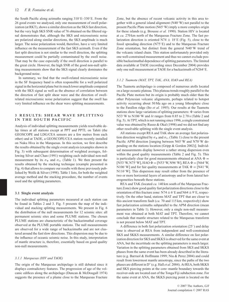
the South Pacific along azimuths ranging 310◦E–330◦E. From the26 good events we analysed, only one measurement of swell polar-ization (at RKT), shows a similar direction as the SKS fast direction,but the very high SKS SNR value of 76 obtained on the filtered sig-nal demonstrates that, although the SKS and microseismic noiseare polarized along similar directions, the SKS amplitude is muchlarger. The noise polarization would, therefore, have a very limitedinfluence on the measurement of the fast SKS azimuth. Even if thefast split direction is not similar to the swell direction, the splittingmeasurement could be partially contaminated by the swell noise.That may be the case especially if the swell direction is parallel tothe great circle. However, the high SNR of the good non-null split-ting measurements show that the SKS signal clearly dominates thebackground noise.
In summary, we find that the swell-related microseismic noisein the SF frequency band is often responsible for a well polarizedsignal in the horizontal plane but its much lower amplitude comparedwith the SKS signal as well as the absence of correlation betweenthe direction of fast split shear wave and the direction of swell-related microseismic noise polarization suggest that the swell hasvery limited influence on the shear wave splitting measurements.
3 R E S U LT S : S H E A R WAV E S P L I T T I N GI N T H E S O U T H PA C I F I C
Analysis of individual splitting measurements yields resolvable de-lay times at all stations except at PPT and PPTL on Tahiti (theGEOSCOPE and LDG/CEA sensors are a few metres from eachother) and at TAOE, a GEOSCOPE/CEA station recently installedon Nuku Hiva in the Marquesas. In this section, we first describethe results obtained by the single event analysis (examples shown inFig. 3) with subsequent determination of weighted averages, fol-lowing Silver and Chan (1991) weighting each individual non-nullmeasurement by its σ� and σδ t (Table 1). We then present theresults obtained by the stacking technique (example presented inFig. 4) that allows to compare our results with those previously pub-lished by Wolfe & Silver (1998). Table 1 lists, for both the weightedaverage method and the stacking procedure, the number of eventsused and the splitting parameters.
3.1 Single event analysis
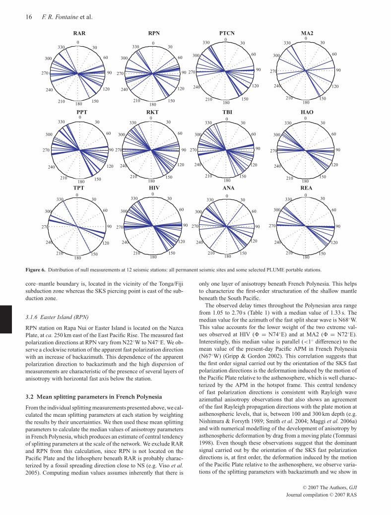
The individual splitting parameters measured at each station canbe found in Tables 2 and 3. Fig. 5 presents the map of the indi-vidual and stacking splitting measurements. We present in Fig. 6the distribution of the null measurements for 12 seismic sites: allpermanent seismic sites and some PLUME stations. The chosenPLUME stations are characteristic of the backazimuthal coverageobserved at the PLUME portable stations. The null measurementsare observed for a wide range of backazimuths and are not clus-tered around the fast/slow directions. This dispersion may be due tothe influence of oceanic seismic noise. In this study, interpretationof mantle structure is, therefore, essentially based on good qualitynon-null measurements.
3.1.1 Marquesas (HIV and TAOE)
The origin of the Marquesas archipelago is still debated since itdisplays contradictory features. The progression of age of the vol-canic edifices along the archipelago (Duncan & McDougall 1974)suggests the presence of a plume close to the Marquesas Fracture
Zone, but the absence of recent volcanic activity in this area to-gether with a general island alignment (N40◦W) not parallel to thepresent Pacific Plate motion (N65◦W) imply a more complex originfor these islands (e.g. Brousse et al. 1990). Station HIV is locatedat ca. 270 km north of the Marquesas Fracture Zone. The fast po-larization direction is oriented N74 ± 18◦E (Fig. 5), close to thefossil spreading direction (N75◦E) and to the Marquesas FractureZone orientation, but distinct from the general N40◦W trend ofthe volcanic island chain. This station unfortunately provided onlyone well-constrained measurement and thus we cannot exclude pos-sible backazimuthal dependence of splitting parameters. The limiteddata available at TAOE (recording since December 2004) providesonly one null measurement at TAOE for a backazimuth of N264◦E.
3.1.2 Tuamotu (MAT, TPT, TAK, ANA, HAO and REA)
The Tuamotu archipelago is composed of numerous atolls locatedon a large oceanic plateau. This plateau trends roughly parallel to thePacific Plate motion but its origin is probably much older than theother Polynesian volcanic alignments, perhaps related to hotspotactivity occurring about 50 Ma ago on a young lithosphere closeto the Farallon ridge (Ito et al. 1995). Our results at the Tuamotustations show large variations of splitting parameters: � varies fromN53◦W to N106◦W and δt ranges from 0.85 to 2.70 s (Table 2 andFig. 5). At TPT, which is not running since 1996, a single constrainedvalue was obtained by Russo & Okal (1998) and we did not find anyother resolvable splitting with the single event analysis.
All stations except REA and TAK show an average fast polariza-tion direction weighted by σ� and σδ t (Table 1) close to the presentPacific APM direction [ranging between N65◦W and N70◦W de-pending on the stations location (Gripp & Gordon 2002)]. Individ-ual measurements display however a rather strong dispersion evenwithin the good quality measurements (Table 2 and Fig. 5). Thisis particularly clear for good measurements obtained at ANA � =[N53◦W, N75◦W], HAO � = [N53◦W, N96◦W], REA � = [N64◦W,N106◦W] and for fair quality measurements at TAK � = [N41◦W,N116◦W]. This dispersion may result either from the presence oftwo or more horizontal layers of anisotropy and/or from lateral het-erogeneities beneath these stations.
REA and TAK (located ca. 140 km south of the Marquesas Frac-ture Zone) show good quality fast polarization directions close to theorientation of this fracture zone: N74 ± 6◦E and N64 ± 9◦E, respec-tively. On the other hand, stations MAT and TPT that are closer tothis ancient transform fault (ca. 70 and 115 km, respectively) showfast polarization azimuths subparallel to the APM direction (meanparameters in Table 1). However, only a single non-null measure-ment was obtained at both MAT and TPT. Therefore, we cannotconclude that mantle structure related to the Marquesas transformis not present below MAT and TPT.
A difference in both fast polarization orientation (25◦) and delaytime is observed at REA from independent and well-constrainedSKS and SKKS measurements. A similar difference on fast polar-ization direction for SKS and SKKS is observed for the same event atANA, but the incertitude on the splitting parameters is much larger.Variation in the splitting parameters obtained from SKS and SKKSphases from the same event has been already described in the litera-ture (e.g. Barruol & Hoffmann 1999; Niu & Perez 2004) and couldresult from lowermost mantle anisotropy, since the paths of the twophases are different in D′′ (e.g. Hall et al. 2004). At REA, both SKKSand SKS piercing points at the core–mantle boundary towards thereceiver-side are located east of the Tonga/Fiji subduction zone. Forthe same event at ANA, the SKKS piercing point is located on the
C© 2007 The Authors, GJI
Journal compilation C© 2007 RAS
June 2, 2007 15:5 Geophysical Journal International gji˙3475
Shear wave splitting beneath French Polynesia 13
6420
-2-46420
-2-4
Before correction After correction
REA, event 2002 11 17, Baz N318.7°E, dist. 95.3°
time (s)Delay time (s)
Azi
mut
h (d
egre
es)
1280 1320 1360 1400 1440 1480
6420
-2-46420
-2-4
SKSac SKKSacSScS
50°E
0°
50°W
0 1 2 3 4
0.5
0.0
-0.5
0.5
0.0
-0.5
4
2
0
-2
-4
-6
1390 1400 1390 1400
-6 -4 -2 0 2 4
Radialafter correction
Transverseafter correction
Transverse
Radial
fast
slow slow
time (s) time (s)
2
0-2
2
0-2
2
0-2
2
0-2
1355 1365 1375 1355 1365 1375
HAO, event 2004 06 10, Baz N330.9˚E, dist. 88.7˚
time (s) Delay time (s)
Azi
mut
h (d
egre
es)
2
0
-2
2
0
-2
2
0
-2
2
0
-2
SKiKP SKSac
2 3 40 1
50°E
0°
50°W
0.5
0.0
-0.5
-1.0
0.5
0.0
-0.5
-1.01418 1422 1426 1418 1422 1426
2
1
0
-1
-2
2
1
0
-1
-2-2 -1 0 1 2 -2 -1 0 1 2
Before correction After correction
slow slow
fast
time (s) time (s)
SKKSac
SScS
1300 1340 1380 1420 1460 1500
Radialafter correction
Transverseafter correction
Transverse
Radial
HAO, event 2005 02 05, Baz N273˚E, dist. 97˚
time (s) Delay time (s)
Azi
mut
h (d
egre
es)
SKSac SKKSac
1240 1280 1320 1360 1400 1440
slow slow
fast
2 3 40 1
50°E
0°
50°W
1.0
0.5
0.0
-0.5
1.0
0.5
0.0
-0.5
2
0
-2
2
0
-2
-2 0 2 -2 0 2
time (s) time (s)
Before correction After correction
Radialafter correction
Transverseafter correction
Transverse
Radial
RKT, event 2004 07 25, Baz N254.3˚E, dist. 117.2˚
time (s)Delay time (s)
Azi
mut
h (d
egre
es)
2 3 40 1
50°E
0°
50°W
SKSacSKSdf SKKSac
5
0
-5
5
0
-5
5
0
-5
5
0
-5
1900 1940 1980 2020 2060 2100 slow slow
fast
time (s)
Before correction After correction
0.5
0.0
-0.5
-1.0
0.5
0.0
-0.5
-1.02025 2035 2045 2025 2035 2045
time (s)4
2
0
-2
-4
-6
4
2
0
-2
-4
-6-6 -4 -2 0 2 4 -6 -4 -2 0 2 4
Radialafter correction
Transverseafter correction
Transverse
Radial
-6 -4 -2 0 2 4
4
2
0
-2
-4
-6
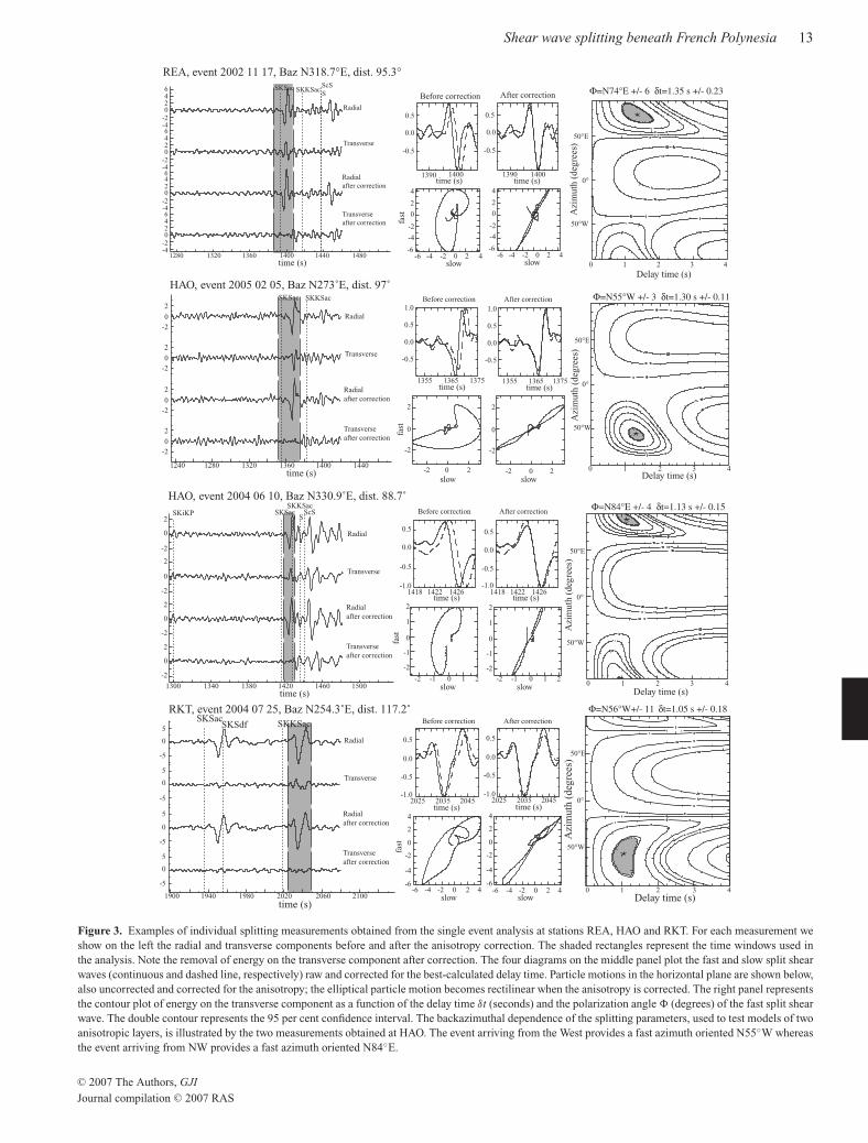
Figure 3. Examples of individual splitting measurements obtained from the single event analysis at stations REA, HAO and RKT. For each measurement weshow on the left the radial and transverse components before and after the anisotropy correction. The shaded rectangles represent the time windows used inthe analysis. Note the removal of energy on the transverse component after correction. The four diagrams on the middle panel plot the fast and slow split shearwaves (continuous and dashed line, respectively) raw and corrected for the best-calculated delay time. Particle motions in the horizontal plane are shown below,also uncorrected and corrected for the anisotropy; the elliptical particle motion becomes rectilinear when the anisotropy is corrected. The right panel representsthe contour plot of energy on the transverse component as a function of the delay time δt (seconds) and the polarization angle � (degrees) of the fast split shearwave. The double contour represents the 95 per cent confidence interval. The backazimuthal dependence of the splitting parameters, used to test models of twoanisotropic layers, is illustrated by the two measurements obtained at HAO. The event arriving from the West provides a fast azimuth oriented N55◦W whereasthe event arriving from NW provides a fast azimuth oriented N84◦E.
C© 2007 The Authors, GJI
Journal compilation C© 2007 RAS
June 2, 2007 15:5 Geophysical Journal International gji˙3475
14 F. R. Fontaine et al.
SKS
2004 06 10 Baz = 328.9
SKKS
2004 07 25 Baz = 254.3
1996 01 01 Baz = 264.7
SKS
1995 12 25 Baz = 261.4
SKKS
SKS
2001 01 01 Baz = 273.1
SKS
2001 01 02 Baz = 273.0
SKS
2001 10 19 Baz = 261.8
Delay time (s)
Azi
mut
h (d
egre
es)
Before correction After correction Before correction After correction
Before correction After correction
time (s) time (s)
time (s) time (s)
time (s) time (s)
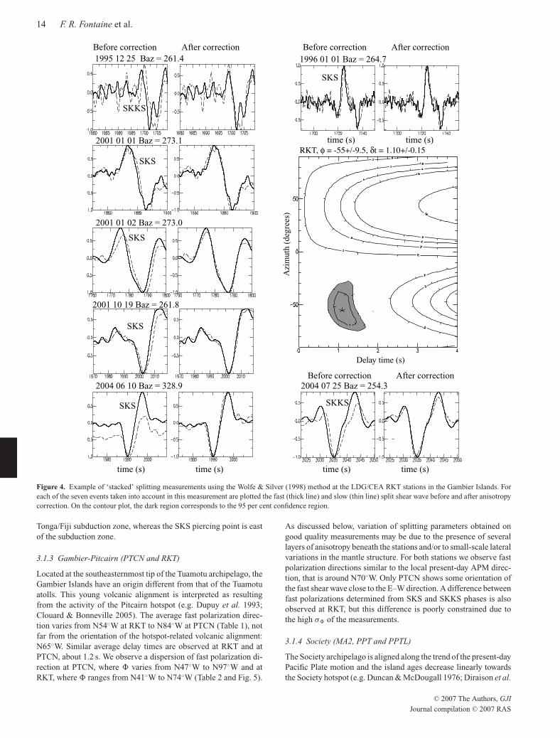
Figure 4. Example of ‘stacked’ splitting measurements using the Wolfe & Silver (1998) method at the LDG/CEA RKT stations in the Gambier Islands. Foreach of the seven events taken into account in this measurement are plotted the fast (thick line) and slow (thin line) split shear wave before and after anisotropycorrection. On the contour plot, the dark region corresponds to the 95 per cent confidence region.
Tonga/Fiji subduction zone, whereas the SKS piercing point is eastof the subduction zone.
3.1.3 Gambier-Pitcairn (PTCN and RKT)
Located at the southeasternmost tip of the Tuamotu archipelago, theGambier Islands have an origin different from that of the Tuamotuatolls. This young volcanic alignment is interpreted as resultingfrom the activity of the Pitcairn hotspot (e.g. Dupuy et al. 1993;Clouard & Bonneville 2005). The average fast polarization direc-tion varies from N54◦W at RKT to N84◦W at PTCN (Table 1), notfar from the orientation of the hotspot-related volcanic alignment:N65◦W. Similar average delay times are observed at RKT and atPTCN, about 1.2 s. We observe a dispersion of fast polarization di-rection at PTCN, where � varies from N47◦W to N97◦W and atRKT, where � ranges from N41◦W to N74◦W (Table 2 and Fig. 5).
As discussed below, variation of splitting parameters obtained ongood quality measurements may be due to the presence of severallayers of anisotropy beneath the stations and/or to small-scale lateralvariations in the mantle structure. For both stations we observe fastpolarization directions similar to the local present-day APM direc-tion, that is around N70◦W. Only PTCN shows some orientation ofthe fast shear wave close to the E–W direction. A difference betweenfast polarizations determined from SKS and SKKS phases is alsoobserved at RKT, but this difference is poorly constrained due tothe high σ� of the measurements.
3.1.4 Society (MA2, PPT and PPTL)
The Society archipelago is aligned along the trend of the present-dayPacific Plate motion and the island ages decrease linearly towardsthe Society hotspot (e.g. Duncan & McDougall 1976; Diraison et al.
C© 2007 The Authors, GJI
Journal compilation C© 2007 RAS
June 2, 2007 15:5 Geophysical Journal International gji˙3475
Shear wave splitting beneath French Polynesia 15
195° 200° 205° 210° 215° 220° 225° 230° 235° 240° 245° 250° 255°
-30°
-25°
-20°
-15°
-10°
-5°
-30°
-25°
-20°
-15°
-10°
-5°20
20
40
40
40
60
60
80
100
100
Pacificplate motion
Nazca
Pacificplate motion
Nazca
-6400-6000-5600-5200-4800-4400-4000-3600-3200-2800-2400-2000-1600-1200-800-400
0depth (m)
195˚ 200˚ 205˚ 210˚ 215˚ 220˚ 225˚ 230˚ 235˚ 240˚ 245˚ 250˚ 255˚20
20
40
40
60
60
80
80
100
100
ANA
HAO
HIV
MA2MAT
RAI
RAP
REA
RUR
TAK
RKTTBI
PPT
PTCN
RAR
RPN
Pacificplate motion
Pacificplate motion
HIV
TAK
PTCN
RKTRAI
TBIRUR
TPTMAT
MA2PPT ANA
HAO
REA
TPT
RAR
a
b
RPN
Marquesas
Society
Australs
Cook
Gambier Pitcairn
Marquesas
Tuamotu
Society
Cook
Australs
GambierPitcairn
TAOE
RAP
Tuamotu
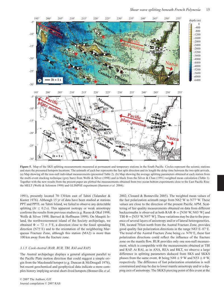
Figure 5. Map of the SKS splitting measurements measured at permanent and temporary stations in the South Pacific. Circles represent the seismic stationsand stars the presumed hotspots locations. The azimuth of each bar represents the fast split direction and its length the delay time between the two split arrivals.(a) Map showing all the non-null individual measurements (presented Table 2). (b) Map showing the average splitting parameters obtained at each station fromthe multi-event stacking technique (grey bars) from Wolfe & Silver (1998) and in black from the Silver & Chan (1991) weighted mean calculation (Table 1).Together with the new results from the present paper are plotted the measurements obtained from two ocean bottom experiments close to the East Pacific Rise:the MELT (Wolfe & Solomon 1998) and GLIMPSE experiment (Harmon et al. 2004).
1991), presently located 70–130 km east of Tahiti (Talandier &Kuster 1976). Although 15 yr of data have been studied at stationsPPT and PPTL on Tahiti Island, we failed to observe any detectablesplitting (δt ≤ 0.2 s). This apparent isotropy or weak anisotropyconfirms the results from previous studies (e.g. Russo & Okal 1998;Wolfe & Silver 1998; Barruol & Hoffmann 1999). On Maupiti Is-land, the northwesternmost island of the Society archipelago, weobtained � = 72 ± 5◦E, a direction close to the fossil spreadingdirection (N75◦E) and to the orientation of the neighboring Mar-quesas Fracture Zone, although this station (MA2) is more than100 km away from the fracture zone.
3.1.5 Cook-Austral (RAR, RUR, TBI, RAI and RAP)
The Austral archipelago displays a general alignment parallel tothe Pacific Plate motion direction that could suggest a simple ori-gin from the Macdonald hotspot (e.g. Duncan & McDougall 1976),but recent geochemical and geophysical data indicate a more com-plex history implying several short-lived hotspots (Bonneville et al.
2002; Clouard & Bonneville 2005). The weighted mean values ofthe fast polarization azimuth range from N62◦W to N77◦W. Thesevalues are close to the direction of the present Pacific APM. Scat-tering of fair quality measurements obtained on data from differentbackazimuths is observed at both RAR � = [N30◦W, N83◦W] andTBI �= [N53◦W, N97◦W]. These variations may be due to the pres-ence of several layers of anisotropy and/or of lateral heterogeneities.TBI, located 70 km north from the Austral Fracture Zone, providesgood quality fast polarization directions in the range N83◦E–87◦E.The trend of the Austral Fracture Zone being ca. N70◦E, these fastpolarization directions could reflect the influence of the fracturezone on the mantle flow. RUR provides only one non-null measure-ment, which is compatible with the measurements obtained at TBIand RAP. At RAI, as in ANA, REA and RKT, we observe a largedifference in splitting parameters deduced from SKS and SKKSphases from the same event, � being N88 ± 9◦W and N53 ± 8◦W,respectively. The difference of fast polarization orientation is wellconstrained and may be due to lower mantle anisotropy and/or a dip-ping axis of anisotropy. The SKKS piercing point of this event at the
C© 2007 The Authors, GJI
Journal compilation C© 2007 RAS
June 2, 2007 15:5 Geophysical Journal International gji˙3475
16 F. R. Fontaine et al.
PPT RKT TBI
TPT REA
RPN
HIV ANA
MA2
030
60
90
120
150180210
240
270
300
3300
330 30
60
90
120
150180
210
240
270
300
030
60
90
330
120
150180
210
240
270
300
030
60
90
120
150180210
240
270
300
3300
30
60
90
120
150180
330
300
270
240
210
030
60
90
120
150180
330
300
270
240
210
030
180150
120
90
60
210
240
270
300
3300
30330
60
90
120
150180
210
240
270
300
030
60
90
120
150180
210
240
270
300
330
030
60
90
120
150180
210
240
270
300
330
030
60
90
120
150180
210
240
270
300
330
030
60
90
120
150180
210
240
270
300
330
RAR PTCN
HAO
Figure 6. Distribution of null measurements at 12 seismic stations: all permanent seismic sites and some selected PLUME portable stations.
core–mantle boundary is, located in the vicinity of the Tonga/Fijisubduction zone whereas the SKS piercing point is east of the sub-duction zone.
3.1.6 Easter Island (RPN)
RPN station on Rapa Nui or Easter Island is located on the NazcaPlate, at ca. 250 km east of the East Pacific Rise. The measured fastpolarization directions at RPN vary from N22◦W to N47◦E. We ob-serve a clockwise rotation of the apparent fast polarization directionwith an increase of backazimuth. This dependence of the apparentpolarization direction to backazimuth and the high dispersion ofmeasurements are characteristic of the presence of several layers ofanisotropy with horizontal fast axis below the station.
3.2 Mean splitting parameters in French Polynesia
From the individual splitting measurements presented above, we cal-culated the mean splitting parameters at each station by weightingthe results by their uncertainties. We then used these mean splittingparameters to calculate the median values of anisotropy parametersin French Polynesia, which produces an estimate of central tendencyof splitting parameters at the scale of the network. We exclude RARand RPN from this calculation, since RPN is not located on thePacific Plate and the lithosphere beneath RAR is probably charac-terized by a fossil spreading direction close to NS (e.g. Viso et al.2005). Computing median values assumes inherently that there is
only one layer of anisotropy beneath French Polynesia. This helpsto characterize the first-order structuration of the shallow mantlebeneath the South Pacific.
The observed delay times throughout the Polynesian area rangefrom 1.05 to 2.70 s (Table 1) with a median value of 1.33 s. Themedian value for the azimuth of the fast split shear wave is N68◦W.This value accounts for the lower weight of the two extreme val-ues observed at HIV (� = N74◦E) and at MA2 (� = N72◦E).Interestingly, this median value is parallel (<1◦ difference) to themean value of the present-day Pacific APM in French Polynesia(N67◦W) (Gripp & Gordon 2002). This correlation suggests thatthe first order signal carried out by the orientation of the SKS fastpolarization directions is the deformation induced by the motion ofthe Pacific Plate relative to the asthenosphere, which is well charac-terized by the APM in the hotspot frame. This central tendencyof fast polarization directions is consistent with Rayleigh waveazimuthal anisotropy observations that also shows an agreementof the fast Rayleigh propagation directions with the plate motion atasthenospheric levels, that is, between 100 and 300 km depth (e.g.Nishimura & Forsyth 1989; Smith et al. 2004; Maggi et al. 2006a)and with numerical modelling of the development of anisotropy byasthenospheric deformation by drag from a moving plate (Tommasi1998). Even though these observations suggest that the dominantsignal carried out by the orientation of the SKS fast polarizationdirections is, at first order, the deformation induced by the motionof the Pacific Plate relative to the asthenosphere, we observe varia-tions of the splitting parameters with backazimuth and we show in
C© 2007 The Authors, GJI
Journal compilation C© 2007 RAS
June 2, 2007 15:5 Geophysical Journal International gji˙3475
Shear wave splitting beneath French Polynesia 17
the following of this paper that these variations are consistent withtwo-layer models of anisotropy which could explained up to 44 percent of the observed variations.
3.3 Multiple events investigation
As explained above, the ‘stacking’ technique takes into account sev-eral events to find the best � and δt parameters compatible with theindividual measurements. Stations displaying backazimuthal depen-dence of the splitting parameters have, however, to be consideredwith care since this method may then provide unrealistic averagesof the splitting parameters. This technique has been shown howeverto be useful in oceanic environments (Wolfe & Silver 1998) since(i) the microseismic noise is generally rather high and may hide thesmall transverse component of the split phase, (ii) some stationsdo not provide any resolved splitting with the single event method(such as PPT) and (iii) other stations provide a very limited num-ber of well constrained measurements (such as HIV, MA2, MAT,TPT and RUR). The results obtained from this stacking techniqueare summarized in Table 1. They show similar results to the Silver& Chan (1991) average values, except at RPN, RAI and RUR forwhich large differences ranging from 22◦ to 49◦ are found.
The multiple events procedure yielded results at RAR and RPNstations (Table 1) similar to previous SKS splitting measurements byWolfe & Silver (1998) and to the fast polarization azimuth deducedfrom P-wave polarization deviations at RPN (Schulte-Pelkum et al.2001). Our measurements at TBI, RKT and TPT are consistent withthose of Russo & Okal (1998). However, at PTCN, our fast directionis hardly compatible (difference of 49◦) with their observation. Suchdifference could be due to the fact that we use more events thanthese authors, and particularly three recent events that provide goodquality measurements with � trending EW, but also that we didnot take into account any direct S phases in the stacking procedure.The apparent isotropy we observe at PPT was already described byprevious studies using both the stacking (Russo & Okal 1998; Wolfe& Silver 1998) or the single event methods (Barruol & Hoffmann1999).
In the following discussion, we will only consider the results fromsingle event analysis as we have seen that the presence of multipleanisotropic layers is possible beneath French Polynesia.
4 D I S C U S S I O N
4.1 Possible causes of seismic anisotropy in oceanic basins
The simplest model to explain the development of a pervasive fab-ric (or olivine crystal preferred orientations) invokes shearing of thesublithospheric mantle in response to a velocity gradient between theplate (rigid lithosphere) and the asthenosphere. Progressive coolingof the plate freezes the olivine crystal preferred orientation (CPO)within the plate and results in deepening of the shear zone. This pro-cess aligns the olivine [100] axes, and, therefore, the polarization ofthe fast split shear waves parallel to the absolute plate motion direc-tion. In this model, the observed delay times should thus increasewith lithospheric age (Tommasi 1998). This simple model is prob-ably not fully appropriate for the Pacific, which suffered an impor-tant plate reorganization at the end of Cretaceous (Mammerickx &Sharman 1988; Mayes et al. 1990) and changes in the spreading di-rection during the Oligocene (e.g. Mayes et al. 1990). Variationsin the APM direction are expected to create different layers ofanisotropy, the most superficial one corresponding to the older plate
motion and the deepest corresponding to the present-day astheno-spheric flow (Tommasi 1998; Rumpker et al. 1999). The boundarybetween the two anisotropic layers should lie within the lithosphere,its depth depending on the age of the lithosphere at the time of thechange in plate motion. The sublithospheric mantle may be in mo-tion which means that the fast polarization direction is parallel to thevector difference of the lithosphere and the sublithospheric mantlemotion (Silver et al. 2001).
Transform faults may locally perturb the asthenospheric flowsince they represent a vertical boundary between lithospheres ofdifferent ages and, therefore, of different thicknesses that may lo-cally channel the sublithospheric flow (Sleep 2002). Hotspot activityand the related mantle upwelling should also modify the sublitho-spheric flow. Indeed, the rising mantle material may spread beneaththe moving lithosphere. The interaction between the upwelling man-tle and the horizontal displacement of the lithosphere is proposed toinduce a parabolic asthenospheric flow (Ribe & Christensen 1994),which should be visible in the shear wave splitting measurements ifthe station coverage is dense enough (Walker et al. 2005b). The geo-metrical characteristics of this parabolic flow depend on the velocityof the plate motion and also on the strength of the plume-inducedmantle flux (Ribe & Christensen 1994; Ribe & Christensen 1999).The presence of penetrative partial melt could also produce addi-tional anisotropy in the sublithospheric mantle due to an alignmentof melt-rich domains or result in a change in olivine deformationpatterns (Holtzman et al. 2003; Fontaine et al. 2005). In addition,it has been proposed that mantle plumes may locally destroy or atleast modify the lithospheric anisotropy by reheating and thinningof the lithosphere (Sleep 1994; Thoraval et al. 2006). Melt-rockinteraction in the lithospheric mantle, on the other hand, should pre-serve seismic anisotropy, except in local melt accumulation horizons(Tommasi et al. 2004).
4.2 Comparison with previous seismic measurementsof anisotropy in the Pacific
Seismic refraction experiments performed few decades ago in thenorthern Pacific yielded Pn azimuthal anisotropy, with fast P-wavevelocities parallel to the transform faults and normal to the mag-netic lineation, that is, parallel to the palaeospreading direction,suggesting alignment of the olivine [100] axes at high angle fromthe ridge trend by the asthenospheric flow (Hess 1964). These fastPn directions are roughly EW north of Hawaii (Hess 1964; Francis1969; Raitt et al. 1969) and close to N150◦E in the northwesternpart of the Pacific (Shimamura & Asada 1983). Since seismic re-fraction uses Pn waves travelling within the uppermost part of thelithospheric mantle, this technique is unable to provide informationon the deeper structure of the lithosphere and on the asthenosphericflow that could correspond to the present-day plate motion.
Splitting of teleseismic shear waves has been measured at severalplaces in the Pacific basin. In Hawaii, on a 90 Ma old lithosphere, theSKS splitting observations obtained at the GEOSCOPE station KIP(Wolfe & Silver 1998; Barruol & Hoffmann 1999; Walker et al.2001) provide results compatible with two layers of anisotropy, alower layer with a fast azimuth parallel to the present-day PacificAPM direction and an upper layer with a fast azimuth close to thepalaeospreading direction, therefore, compatible with the fast Pndirections. Experiments deployed in the vicinity of the East PacificRise show primarily fast shear wave polarizations parallel to thepresent spreading direction (Wolfe & Solomon 1998; Harmon et al.2004). By using splitting of PS phases from deep Tonga eventsrecorded at North American stations, Su & Park (1994) measured
C© 2007 The Authors, GJI
Journal compilation C© 2007 RAS
June 2, 2007 15:5 Geophysical Journal International gji˙3475
18 F. R. Fontaine et al.
a fast anisotropy orientation close to the APM direction. In FrenchPolynesia, Russo & Okal (1998) perform splitting measurementsat four permanent IRIS, GEOSCOPE and CEA/LDG stations andyield NW–SE fast split shear wave directions compatible with anasthenospheric origin, but with rather strong variations from stationto station they attribute to short-scale variations in the upper-mantlepenetrative structure related to the presence of the hotspot in thisarea.
Rayleigh wave azimuthal anisotropy provides a way to globallymap the Pacific upper mantle with a good vertical sensitivity butwith a lateral resolution of several hundreds of kilometres. Theyare, therefore, complementary to SKS waves that have lateral res-olutions of few tens of kilometres but no vertical resolution. Thefirst surface wave anisotropic models derived from few hundredseismic path crossing the Pacific (e.g. Montagner 1985; Nishimura& Forsyth 1988; Nishimura & Forsyth 1989) already showed anazimuthal anisotropy correlated to the palaeospreading direction atshort periods and a better correlation to the present-day plate motionat longer periods, that is, at greater depth. More recent inversionsusing several ten thousands of seismic ray paths provide a betterlateral resolution in the Pacific ocean and confirm the presence oftwo layers of anisotropy (Trampert & Woodhouse 2003; Smith et al.2004), but they also give evidence of lateral variations of velocityand anisotropy that could be related to channeling of mantle flow(Montagner 2002) or to hotspot-related mantle upwelling (Maggiet al. 2006a).
4.3 Fossil anisotropy
As the oceanic plate cools, sublithospheric anisotropy is expectedto be progressively frozen at the bottom of the lithosphere and theshear zone accommodating the velocity gradient between the plateand the deeper asthenosphere is progressively displaced towardslarger depths. If the plate motion direction and velocity are constantthrough time, anisotropy should be homogeneous over the entireplate and sublithospheric mantle (Tommasi 1998).
For the Pacific Plate, the orientation of the present-day APM isclose to the present-day spreading direction and one can assume thatthe same geometrical relationship existed before the plate reorgani-zation that occurred roughly at magnetic anomaly 7 (25–26 Ma),(e.g. Mayes et al. 1990). In this simple model, the lithosphericstrain for old (>25 Ma) French Polynesia seafloor, and therefore,the olivine [100] axes, should align close to the palaeoexpansiondirection, underlined by the fracture zones.
In the South Pacific, the Marquesas and the Austral FractureZones are oriented N75◦E and underline the Pacific-Farallon spread-ing direction between 100 and 25 Ma. At the proximity of the fracturezones (TBI, TAK, MA2 and HIV) some fast directions (ranging be-tween N64◦E and N83◦E) are observed to be close to the orientationof this frozen tectonic structure, consistent with the presence of afossil anisotropy in the uppermost mantle. At larger distance fromthe fracture zones, as for instance at HAO, REA and PTCN, we alsoobserve some fast polarization directions close to the palaeospread-ing direction (between N74◦E and N85◦E), suggesting that a ENEfossil anisotropy is pervasively present in the lithosphere beneathFrench Polynesia.
4.4 Testing two-layer models: forward approach
The presence of several layers of anisotropy with horizontal fast di-rections beneath a given station is expected to produce an azimuthal
variation of the splitting parameters � and δt that are obtained underthe assumption of a single anisotropic layer (Silver & Savage 1994;Rumpker et al. 1999). Such a structure may, therefore, explain theapparent scattering observed at the South Pacific seismic stations.In the Pacific Ocean, two-layer models have been already proposedto explain the apparent variation of splitting parameters observedat station KIP on Oahu Island (Wolfe & Silver 1998; Barruol &Hoffmann 1999; Walker et al. 2001). As pointed out by previousstudies (e.g. Hartog & Schwartz 2001), it is theoretically not pos-sible to determine a unique model from observations of apparentsplitting parameters without independent constraints. However, useof a priori geophysical constraints, as for instance the plate mo-tion direction, allows determining families of plausible geodynamicmodels.
In order to compensate for the small number of events for test-ing the presence of two anisotropic layers beneath French Polyne-sia, we group the splitting observations over the entire network.This appears appropriate since a two-layer modelling requires bet-ter backazimuth coverage than we have at each individual station,and also since we want to decrease the influence of the seismicnoise that is inherent in all the individual measurements. Indeed,we observe homogeneous fast split shear wave directions across thenetwork for each range of event backazimuths (Fig. 7). We use a for-ward approach to evaluate the presence of two layers of anisotropybeneath French Polynesia considering measurements obtained forfive events which provide evidence of splitting at several stationstogether (RAI, ANA, MA2, TAK, REA, PTCN, HAO, RAP, TBI,RUR and RKT). When two different measurements were availablefor the same event and at the same station for both SKS and SKKSphases, we decided to use the best-constrained measurement (lowestincertitude of both � and δt). We do not include in this approachresults from RPN (on the Nazca Plate) and RAR [much older litho-sphere with fossil spreading direction presumed to be close to NS(Viso et al. 2005)]. The present Pacific APM directions at the var-ious seismic stations in French Polynesia range from N65◦W andN72◦W (e.g. Gripp & Gordon 2002), and the fossil spreading direc-tion using magnetic isochrons is N75◦E (e.g. Muller et al. 1997). Weperform a grid search over the four parameters (� and δt for boththe upper and lower layers) to determine the optimum model thatmay explain the observed backazimuthal variations of the splittingparameters. Following the scheme described by Silver & Savage(1994) and for a dominant signal frequency of 0.1 Hz, we computethe apparent splitting backazimuthal variation for each two-layermodel, by varying in each layer the fast directions in steps of 2◦
(from 0◦E to 180◦E) and the delay time by steps of 0.2 s (from 0to 2.6 s, which is our maximum observed value of delay time), pro-viding a total of 1 353 690 models. To determine the ‘best-fitting’model we have computed an appropriate misfit function for the twosets of parameters,
∑(�observed − �calculated)2/σ 2
� + ∑(δtobserved
− δtcalculated)2/σ 2δ t. The ratio of that function with respect to the
one for the best-fitting model (�opt, δtopt) follows an F distribution,from which we determine the range of parameters that are within the95 per cent confidence region, and thus acceptable. For each model,we also calculated the coefficient of determination R2. As mentionedby Walker et al. (2004) the goal of R2 is to estimate the degree towhich two-layer models fit the splitting observations better than asingle-layer model with horizontal fast axis.
R2 = 1 − SSd/SSo, (1)
where SSd is a sum of squares of the two-layer model misfit andSSo a sum of squares of the single-layer model (with horizontal
C© 2007 The Authors, GJI
Journal compilation C© 2007 RAS

June 2, 2007 15:5 Geophysical Journal International gji˙3475
Shear wave splitting beneath French Polynesia 19
-30˚
-20˚
-10˚
80
85
90
100
110
70
80
85
90
100
-30˚
-20˚
-10˚ 80
85
90
100
1 10
70
80
85
85
90
100
200˚ 210˚ 220˚ 230˚-30˚
-20˚
-10˚
70
80
90100
200˚ 210˚ 220˚ 230˚210˚ 220˚
1000
110
120
a
c
e
b
d
f
HIV
REA
PPT
PTCN
RAR
RAP
HIV
REAPPT
PTCN
RAR
RAP
HIV
REA
PPT
PTCNRAR
RAP
HIV
PPT
PTCN
RAR
RAP
HIV
REAPPT
PTCNRAR
RAP
HIV
REAPPT
PTCN
RAR
RAP
RAITBI
MA2MAT
ANA
TAK
HAO
ANA
RAITBI
MA2
REA
RAI
RUR RURTBI
RAI
MAT
ANA
MAT
ANAHAO
RUR
TAKMAT
Event#3 Kuriles 2002 11 17 04h53 - Baz ≈ N320°
Event#5 Philippines 2003 05 26 23h13 - Baz ≈ N275° Event#2 Kamchatka 2003 06 16 22h08 - Baz ≈ N330°
Event#4 Kamchatka 2004 06 10 15h19 - Baz ≈ N330° Event#1 Sumatra 2004 07 25 14h35 - Baz ≈ N260°
Event#6 Taiwan 2002 03 31 06h52 - Baz ≈ N290°
MA2
TAK
HAO
HAO
RKT RKT
HAO
ANA
RKT
HAO
Figure 7. Maps of individual splitting measurements obtained at the PLUME and permanent stations for 6 particular events, sorted chronologically from (a)to (f). Circles represent the seismic stations and stars the presumed hotspots locations. The azimuth of the measured fast split direction is marked by the blackline, and its length is proportional to the delay time. The maps also show the epicentral distances from the respective events. For some events, the minimum 85◦epicentral distance is located in the middle of the network, explaining the absence of measurements at some stations located too close to the event. The Taiwanevent (a) (backazimuth N293◦E) provides high quality signals with consistently absent signal energy on the transverse component across the network (nullmeasurements). The corresponding waveforms were already published in Barruol et al. (2002). This figure shows that the fast split directions are dependent onthe event backazimuth, with fast directions trending ENE–WSW for backazimuths of N320◦E (b) and NW–SE for backazimuths of N260◦E (f).
axis).
SSd =∑N
1
[((�observed − �2 layer)
σ�
)2
+(
(δtobserved − δt2 layer)
σδt
)2]
(2)
and
SSo =∑N
1
[((�observed − �1 layer)
σ�
)2
+(
(δtobserved − δt1 layer)
σδt
)2]
(3)
σ� and σδt are the standard deviations of observed splitting pa-rameters and N is the number of splitting measurements (i.e. 28in our case). R2 is the fraction of the total sum of squares that is
explained. Theoretically and without the presence of seismic noise,this value ranges from 0 (no improvement by the two-layer model) to1 (perfect fit). However, this number can be negative if the misfitof the single-layer model is lower than the misfit of the two-layermodel. The determination coefficient can be biased by the numberof independent variables. We therefore, compute a better coefficient,the adjusted R2:
R2adjusted = 1 − (Nd − 1)(1 − R2)/(Nd − k − 1), (4)
where Nd is the number of observations (i.e. 2∗N) and k is the numberof model parameters. This value is an index and can vary from −∞to 1. As is done by Walker et al. (2005a) we consider as statistically
C© 2007 The Authors, GJI
Journal compilation C© 2007 RAS
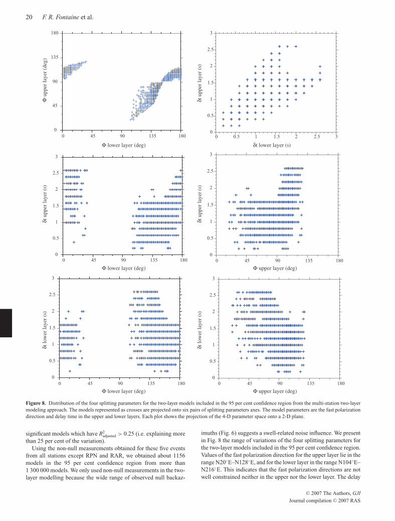
June 2, 2007 15:5 Geophysical Journal International gji˙3475
20 F. R. Fontaine et al.
0
45
90
135
180
0 45 90 135 180
(s)
0
0.5
1
1.5
2
2.5
3
0 45 90 135 180
(s)
(s)
(s)
(s)
(s)
0
0.5
1
1.5
2
2.5
3
0 0.5 1 1.5 2 2.5 3
0
0.5
1
1.5
2
2.5
3
0 45 90 135 180
0
0.5
1
1.5
2
2.5
3
0 45 90 135 1800
0.5
1
1.5
2
2.5
3
0 45 90 135 180
Figure 8. Distribution of the four splitting parameters for the two-layer models included in the 95 per cent confidence region from the multi-station two-layermodeling approach. The models represented as crosses are projected onto six pairs of splitting parameters axes. The model parameters are the fast polarizationdirection and delay time in the upper and lower layers. Each plot shows the projection of the 4-D parameter space onto a 2-D plane.
significant models which have R2adjusted > 0.25 (i.e. explaining more
than 25 per cent of the variation).Using the non-null measurements obtained for these five events
from all stations except RPN and RAR, we obtained about 1156models in the 95 per cent confidence region from more than1 300 000 models. We only used non-null measurements in the two-layer modelling because the wide range of observed null backaz-
imuths (Fig. 6) suggests a swell-related noise influence. We presentin Fig. 8 the range of variations of the four splitting parameters forthe two-layer models included in the 95 per cent confidence region.Values of the fast polarization direction for the upper layer lie in therange N20◦E–N128◦E, and for the lower layer in the range N104◦E–N216◦E. This indicates that the fast polarization directions are notwell constrained neither in the upper nor the lower layer. The delay
C© 2007 The Authors, GJI
Journal compilation C© 2007 RAS
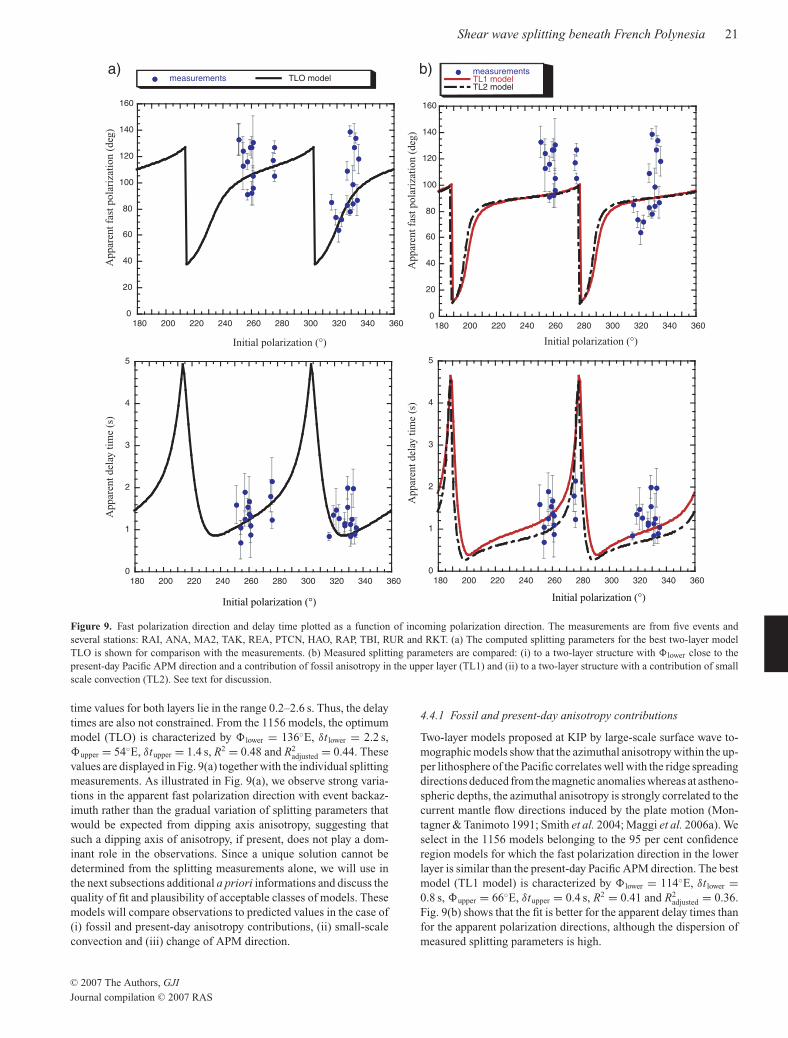
June 2, 2007 15:5 Geophysical Journal International gji˙3475
Shear wave splitting beneath French Polynesia 21
0
20
40
60
80
100
120
140
160
180 200 220 240 260 280 300 320 340 360
measurements TLO model
0
1
2
3
4
5
180 200 220 240 260 280 300 320 340 360
0
20
40
60
80
100
120
140
160
180 200 220 240 260 280 300 320 340 360
measurementsTL1 modelTL2 model
0
1
2
3
4
5
180 200 220 240 260 280 300 320 340 360
a) b)
App
aren
t del
ay ti
me
(s)
App
aren
t fas
t pol
ariz
atio
n (d
eg)
App
aren
t del
ay ti
me
(s)
App
aren
t fas
t pol
ariz
atio
n (d
eg)
Initial polarization (°) Initial polarization (°)
Initial polarization (°)Initial polarization (°) Initial polarization (°)Initial polarization (°)
Figure 9. Fast polarization direction and delay time plotted as a function of incoming polarization direction. The measurements are from five events andseveral stations: RAI, ANA, MA2, TAK, REA, PTCN, HAO, RAP, TBI, RUR and RKT. (a) The computed splitting parameters for the best two-layer modelTLO is shown for comparison with the measurements. (b) Measured splitting parameters are compared: (i) to a two-layer structure with �lower close to thepresent-day Pacific APM direction and a contribution of fossil anisotropy in the upper layer (TL1) and (ii) to a two-layer structure with a contribution of smallscale convection (TL2). See text for discussion.
time values for both layers lie in the range 0.2–2.6 s. Thus, the delaytimes are also not constrained. From the 1156 models, the optimummodel (TLO) is characterized by �lower = 136◦E, δt lower = 2.2 s,�upper = 54◦E, δtupper = 1.4 s, R2 = 0.48 and R2
adjusted = 0.44. Thesevalues are displayed in Fig. 9(a) together with the individual splittingmeasurements. As illustrated in Fig. 9(a), we observe strong varia-tions in the apparent fast polarization direction with event backaz-imuth rather than the gradual variation of splitting parameters thatwould be expected from dipping axis anisotropy, suggesting thatsuch a dipping axis of anisotropy, if present, does not play a dom-inant role in the observations. Since a unique solution cannot bedetermined from the splitting measurements alone, we will use inthe next subsections additional a priori informations and discuss thequality of fit and plausibility of acceptable classes of models. Thesemodels will compare observations to predicted values in the case of(i) fossil and present-day anisotropy contributions, (ii) small-scaleconvection and (iii) change of APM direction.
4.4.1 Fossil and present-day anisotropy contributions
Two-layer models proposed at KIP by large-scale surface wave to-mographic models show that the azimuthal anisotropy within the up-per lithosphere of the Pacific correlates well with the ridge spreadingdirections deduced from the magnetic anomalies whereas at astheno-spheric depths, the azimuthal anisotropy is strongly correlated to thecurrent mantle flow directions induced by the plate motion (Mon-tagner & Tanimoto 1991; Smith et al. 2004; Maggi et al. 2006a). Weselect in the 1156 models belonging to the 95 per cent confidenceregion models for which the fast polarization direction in the lowerlayer is similar than the present-day Pacific APM direction. The bestmodel (TL1 model) is characterized by �lower = 114◦E, δt lower =0.8 s, �upper = 66◦E, δtupper = 0.4 s, R2 = 0.41 and R2
adjusted = 0.36.Fig. 9(b) shows that the fit is better for the apparent delay times thanfor the apparent polarization directions, although the dispersion ofmeasured splitting parameters is high.
C© 2007 The Authors, GJI
Journal compilation C© 2007 RAS
June 2, 2007 15:5 Geophysical Journal International gji˙3475
22 F. R. Fontaine et al.
The best model for a fast anisotropic direction in the lower layerclose to the APM have interestingly an upper layer with a fast direc-tion close to the palaeospreading direction underlined by the frac-ture zones. This idea is in full agreement with the two-layer modelsobserved for instance by surface wave tomography (Montagner &Tanimoto 1991; Smith et al. 2004; Maggi et al. 2006a).
4.4.2 Sublithospheric instabilities
In the case of a ridge axis with transform faults along the spread-ing center, numerical simulations from Morency et al. (2005) showthat after 16 Ma, cold downgoing instabilities may develop at thebase of the lithosphere. The orientation of the EPR ridge is N15◦E.If we assume that these results obtained for plate velocities of 2–4 cm yr–1 are still correct at higher velocities, then the direction ofthe horizontal simple shear in the asthenosphere is mainly perpen-dicular to the ridge: N105◦E in the lower layer. Due to the develop-ment of convection rolls, there is certain variability in the horizontalsimple shear direction at the base of the lithosphere, but the sheardirection is still mostly normal to the ridge axis. Additionally, the3-D numerical simulations of Morency et al. (2005) suggest an up-per layer with a direction between 10 and 20◦E from the orientationof the ridge axis for lithospheric ages between 36 and 72 Ma. Inthe case of the EPR ridge, the direction in the upper layer could bebetween N25◦E and N35◦E. Assuming that similar instabilities aretriggered in the South Pacific with a plate motion faster than theone used in the simulations, the best two-layer model (TL2 model)is characterized by �lower = 106◦E, δt lower = 1 s, �upper = 28◦E,δtupper = 0.4 s, R2 = 0.40 and R2
adjusted = 0.35. The quality of thefit is slightly less good than provided by TL1 model. The appar-ent splitting parameters obtained from this model are illustrated inFig. 9(b) together with the observations.
4.4.3 Change in the APM direction
The bend displayed by the Hawaii-Emperor chain is usually inter-preted as a record of a change in the Pacific APM at ca. 43 Ma.A similar shift is suggested in French Polynesia at the scale of theTarava Seamounts (Clouard et al. 2003), the western part of thechain trends N20◦W and the eastern part N60◦W. We investigatedin the 95 per cent confidence region two-layer models with a fastaxis direction close to the present-day APM direction (±5◦) in thelower layer and �upper in the range N10◦W–N30◦W. However, wefound no model corresponding to these criteria. Thus, as previouslysuggested by Tommasi (1998) a two-layer model of anisotropy asso-ciated with a change in the APM direction from N20◦W to N60◦Wat 43 Ma does not seem adequate to explain the observed variationsin the splitting parameters.
In summary, we cannot find a unique two-layer model, but ourresults suggest as follows.
(1) A two-layer structure of anisotropy explains the apparentsplitting parameters variations better than a single layer with hori-zontal fast axis,
(2) An upper mantle with two layers of anisotropy cannot explainthe totality of the splitting observations.
4.5 Testing plume-related upwelling and parabolicflow patterns
Recent surface wave tomographic models of the Pacific upper mantle(Maggi et al. 2006b) evidenced cylindrical low velocity anomalies
down to at least 400 km depth beneath the Society and Macdonaldhotspots that may result from mantle upwellings. These findingsare compatible with body wave tomographic models described byMontelli et al. (2004) that argue for a Society hotspot rooted inthe lower mantle. These mantle upwellings may spread beneath thelithospheric lid generating a parabolic asthenospheric flow due toa combination of the hotspot radial flow and the shear induced bythe overlying plate displacement (Sleep 1990; Kaminski & Ribe2002). Predictions from a parabolic asthenospheric flow patternwere compared with splitting data near Hawaii (Walker et al. 2001),in the Eifel region (Walker et al. 2005b), in the Yellowstone region(Waite & Schutt 2005) and beneath the Seychelles (Hammond et al.2005). Testing such flow pattern in French Polynesia is unfortu-nately strongly limited by the sparse station coverage that does notprovide the necessary short-scale observations, particularly aroundthe hotspots, necessary to constrain the four parameters character-izing the flow field, that is, the plume strength, the plume centre,the plate velocity and the direction of plate motion. In the case ofa fast-moving plate such as the Pacific Plate, the parabolic flow isexpected to be extremely elongated along the APM direction andonly stations above the mantle upwelling may distinguish such amodel from that of simple asthenospheric flow. Additional stationssuch as the broad-band OBS deployed on the head of the hotspot(Suetsugu et al. 2005) may help to test this model.
4.6 Signature of ancient transform faults
The Marquesas and Austral Fracture zones represent frozen trans-form faults that were active at the Pacific–Farallon spreading ridge.Lithospheric age variation across these features is of 10–16 and5–10 Ma, respectively (e.g. Mayes et al. 1990). In both cases, theolder and therefore, thicker lithosphere lies on the northern sideof the fracture zone. Using a simple assumption that the oceaniclithospheric thickness e is related to the plate age t through a rela-tion such as e = 9.1t0 .5, (e.g. Fowler 1990) with e in km, t in Maand for a thermal diffusivity of 0.804.10−6 m2 s−1, the lithosphericstep between the ridge and a 10 Ma old lithosphere should be about29 km. After 70 Ma, this step should be reduced to ca. 5 km (lowerlithospheric layer in Fig. 10). This value is obviously a maximumestimate since lateral cooling and secondary convection (e.g. Sleep2002) will tend to smooth the thermal gradient leading to a constantlithosphere thickness at old ages (e.g. Dumoulin et al. 2001). Closeto a fracture zone and in the case of a young lithosphere, the astheno-spheric flow beneath the lithosphere may be affected by this localrelief and the orientation of this flow should be deviated towardsthe fracture zone direction. This local reorientation of the flow willdepend on the wavelength of the relief, and therefore, on the age stepacross the fracture zone and on the age of the plate. In the case ofFrench Polynesia, the older plate is leading the younger plate and wecould expect a lower component of along-fracture-zone flow than inthe case of a younger plate leading an older plate. However, somestations may potentially record fracture-zone parallel shear behindthe step. Stations TBI and RAI that lie on both sides of the Australfracture zone display indeed fast split shear waves polarizations de-viating from the APM trend towards the fracture zone orientation.In the Society and Tuamotu archipelagoes, stations MA2 and TAK,both on the southern side of the Marquesas Fracture Zone display �
trending almost parallel to the fracture zone direction, like stationHIV in the Marquesas, north of the Marquesas Fracture Zone. Al-though these observed variations are compatible with two layers ofanisotropy, they may also indicate deviations of the asthenosphericflow by a relief of lithosphere–asthenosphere boundary beneath the
C© 2007 The Authors, GJI
Journal compilation C© 2007 RAS
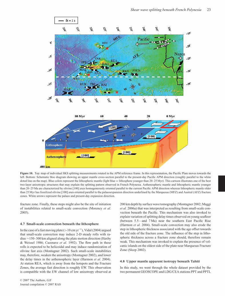
June 2, 2007 15:5 Geophysical Journal International gji˙3475
Shear wave splitting beneath French Polynesia 23
Figure 10. Top: map of individual SKS splitting measurements rotated in the APM reference frame. In this representation, the Pacific Plate moves towards theleft. Bottom: Schematic bloc diagram showing an upper mantle cross-section parallel to the present-day Pacific APM direction (roughly parallel to the whitedoted line on the map). Blue colors represent the lithospheric mantle (light blue = lithosphere younger than 20–25 Myr). This cartoon illustrates one of the besttwo-layer anisotropic structures that may explain the splitting pattern observed in French Polynesia. Asthenospheric mantle and lithospheric mantle youngerthan 20–25 Ma are characterized by olivine [100] axes homogeneously oriented parallel to the current Pacific APM direction whereas lithospheric mantle olderthan 25 Myr has fossilized olivine [100] axes oriented parallel to the palaeoexpansion direction underlined by the Marquesas (MFZ) and Austral (AFZ) fracturezones. White arrows represent the palaeo and present-day expansion direction.
fracture zone. Finally, these steps might also be the site of initiationof instabilities related to small-scale convection (Morency et al.2005).
4.7 Small-scale convection beneath the lithosphere
In the case of a fast moving plate (>10 cm yr–1), Vidal (2004) arguedthat small-scale convection may induce 2-D steady rolls with ra-dius ∼150–300 km aligned along the plate motion direction (Haxby& Weissel 1986; Cazenave et al. 1992). The flow path in theserolls is expected to be helicoidal and may induce randomization ofolivine fast axis (Montagner 2002). Such small-scale instabilitiesmay, therefore, weaken the anisotropy (Montagner 2002), and lowerthe delay times in the asthenospheric layer (Harmon et al. 2004).At station REA, which is away from the hotspots and the FractureZones, the average fast direction is roughly EW. This observationis compatible with the EW channel of low anisotropy observed at
200 km depth by surface wave tomography (Montagner 2002; Maggiet al. 2006a) that was interpreted as resulting from small-scale con-vection beneath the Pacific. This mechanism was also invoked toexplain variation of splitting delay times observed on young seafloor(between 5.5—and 7 Ma) near the southern East Pacific Rise(Harmon et al. 2004). Small-scale convection may also erode thestep in lithospheric thickness associated with the age offset towardsthe old side of the fracture zone. The influence of the step in litho-spheric thickness across a fracture zone should, therefore remainweak. This mechanism was invoked to explain the presence of vol-canic islands on the oldest side of the plate near Marquesas FractureZone (Sleep 2002).
4.8 Upper mantle apparent isotropy beneath Tahiti
In this study, we went through the whole dataset provided by thetwo permanent GEOSCOPE and LDG/CEA stations PPT and PPTL
C© 2007 The Authors, GJI
Journal compilation C© 2007 RAS
June 2, 2007 15:5 Geophysical Journal International gji˙3475
24 F. R. Fontaine et al.
installed on Tahiti and we confirmed the apparent isotropy observedat Tahiti that was already described in several papers during thelast decade (Russo & Okal 1998; Wolfe & Silver 1998; Barruol &Hoffmann 1999). We now discuss four possible causes of apparentisotropy beneath Tahiti, taking into account that a combination ofseveral effects is possible.
4.8.1 Vertical olivine [100] axes
The mantle upwelling beneath a hotspot is expected to concentratethe olivine [100] axes close to the vertical direction. This directionbeing weakly anisotropic within the olivine single crystal (Main-price et al. 2000), this would result in the absence of detectablesplitting by the vertically propagating SKS waves (Mainprice &Silver 1993). The upwelling associated to the Society hotspot israther well resolved in the upper mantle beneath Tahiti by globalbody wave and surface wave tomography (Montelli et al. 2004;Maggi et al. 2006b) that show that the minimum radius of thisplume-like upwelling is 300 km. Since the center of the present-day location of the active Society hotspot is about 130 km ESEfrom Tahiti, one can propose that SKS phases recorded at the Tahitistations sample the Society hotspot mantle upwelling during theirpropagation in the sublithospheric mantle. However, the analysis oflherzolite xenoliths from Tahiti suggests that the lithosphere shouldstill preserve its anisotropy (Tommasi et al. 2004) unless the litho-sphere is mechanically eroded.
4.8.2 Two anisotropic layers
The presence of two anisotropic layers, with perpendicular fast axesand similar δt values in each layer, may in principle also result inthe absence of detectable anisotropy, the delay acquired within thelower layer being removed by the upper one. Such a structure wasproposed for instance at station CAN (Barruol & Hoffmann 1999)and several other stations in Australia (Heintz & Kenneth 2006),but is likely not valid for French Polynesia since the two layers ofanisotropy deduced from SKS splitting, surface waves analyses, andfrom plate tectonics data are clearly not orthogonal to each other.
4.8.3 Presence of melt
The presence of melt in the upper mantle beneath Tahiti may alsoexplain the apparent isotropy. Recent volcanism dated from 1.0 to0.5 Ma is observed on Tahiti Island and surface wave tomographyshows anomalously low upper-mantle velocities beneath the Soci-ety hotspot at depths from 50 to 400 km (Maggi et al. 2006b). Theinfluence of melt on seismic anisotropy is however debated. On onehand, laboratory experiments suggest that the [100] axis alignmentchanges in the presence of melt (e.g. Holtzman et al. 2003). On theother hand, Vauchez & Garrido (2001) have shown from the analysisof olivine preferred orientation in naturally deformed mantle rocksthat the asthenospherization of a lithospheric mantle under staticconditions seems to preserve the original olivine preferred orienta-tions and, therefore, should not affect the seismic anisotropy. Finally,petrophysical modelling combining olivine lattice preferred orien-tation (LPO) and anisometric melt pockets (Vauchez et al. 2000)shows the importance of the relative orientation of the melt pock-ets relative to the solid-state flow microstructure, suggesting thatif melt pockets are oriented at high angle to the foliation the twocontributions may cancel out, providing an isotropic medium for thedirection sampled by the vertically propagating shear wave.
4.8.4 Mantle heterogeneities
The apparent isotropy recorded at Tahiti may finally result from thepresence of small-scale heterogeneities beneath the island that mightconspire to mask the deformation-induced anisotropic signature.Such heterogeneities in the upper-mantle structure can be related tothe magmatism associated to the Society hotspot and/or to small-scale mantle flow variations related to the plume ascent, deflectionand spreading.
5 C O N C L U S I O N
Shear wave splitting measurements were conducted on 18 stations inSouth Pacific and particularly in French Polynesia in the frameworkof the PLUME experiment. The goal was to better document upper-mantle structure and dynamics beneath this poorly instrumentedarea. SKS and SKKS phases sampled an oceanic lithosphere withages varying between 30 and 100 Ma. The observed fast polarizationdirections, at first order, correlate with the present-day Pacific Platemotion direction, suggesting that the anisotropy is primarily relatedto the present-day deformation in the asthenosphere beneath theoceanic plate. At few stations, we observe events with fast polariza-tion directions parallel to fracture zones, suggesting that these fea-tures may have a long-lasting influence on the observed anisotropy.
We show, however, that the fast shear wave polarization direction� depends on event backazimuth and that two layers of anisotropymay explain these variations better than a single layer. Since ourbackazimuthal coverage is not good enough to obtain a unique two-layer anisotropy model, we combine the observations at the networkscale and use additional a priori such as the plate motion directionto constrain the fast polarization azimuth in the lower anisotropiclayer. Our preferred model favours a lower layer of anisotropy re-lated to asthenospheric flow controlled by the absolute plate motionin the hotspot frame and an upper anisotropic layer in the litho-sphere related to the palaeospreading direction between the Pacificand Farallon Plates before 25 Ma (Fig. 10). The presence of a two-layer structure of anisotropy in the South Pacific is consistent withobservations of the azimuthal anisotropy of surface waves.
Second-order variations of the measured splitting parameters arenot explained by apparent � and δt predicted by two-layer models ofanisotropy, suggesting other perturbations such as mantle plumes,small-scale convection and complications with asthenospheric flowassociated with fracture zones.
Despite the availability of a large amount of data (15 yr) at twopermanent stations, no splitting measurements have been obtainedon Tahiti Island. This apparent isotropy or weak anisotropy maybe related to a complex upper-mantle structure induced by the re-cent magmatism on Tahiti and/or a vertical-mantle flow beneath thisisland.
A C K N O W L E D G M E N T S
PLUME has been funded by the French Ministere de la Recherche,Action Concertee Incitative (ACI) jeunes chercheurs and by theMinistere de l’Outre Mer. Many thanks to the Centre National dela Recherche Scientifique (CNRS), to the Government of FrenchPolynesia, to the Universite de Polynesie Francaise (UPF), to theHaut-Commissariat de la Polynesie francaise and to the Commis-sariat a l’Energie Atomique (CEA) for having made possible thisexperiment. Thanks to the Global Seismographic Network (partic-ularly IDA and IRIS/IDA from the University of California, SanDiego and IRIS/USGS from USGS Albuquerque Seismological
C© 2007 The Authors, GJI
Journal compilation C© 2007 RAS
June 2, 2007 15:5 Geophysical Journal International gji˙3475
Shear wave splitting beneath French Polynesia 25
Laboratory) and to GEOSCOPE network (IPG Paris) for the accessi-bility and the quality of their data. The portable seismic stations wereprovided by the Institut National des Sciences de l’Univers (INSU),Reseau Large Bande Mobile (RLBM) managed by J. J. Leveque andJ. Burdin (EOPG Strasbourg). We are extremely thankful to MeteoFrance and to the Aviation Civile for having made possible the in-stallation of seismic stations on their sites and for the useful andefficient help provided by their personnel but also by the munici-palities of the Polynesian Islands. Many thanks to E. Debayle, Y.Vota, B. Jouanneau, A. Vauchez and C. Zaroli for their help in theexperiment. We warmly thank D. Reymond and O. Hyvernaud fromthe CEA in Tahiti for helpful discussions and their help in providingseismic data. We thank K. Walker and an anonymous reviewer forconstructive reviews, M. Sambridge for discussions about modelcomparison and P. Silver for his splitting analysis code. We usedSAC (Lawrence Livermore Nat. Lab) for the seismic analysis andGMT software (SOEST, U. of Hawaıi) for producing the maps.
R E F E R E N C E S
Adam, C.R. & Bonneville, A., 2005. Extent of the South Pacific Superswell,J. Geophys. Res., 110, doi:.
Barruol, G., Silver, P.G. & Vauchez, A., 1997. Seismic anisotropy in theeastern US: deep structure of a complex continental plate, J. Geophys.Res., 102, 8329–8348.
Barruol, G. & Hoffmann, R., 1999. Seismic anisotropy beneath the Geoscopestations from SKS splitting, J. Geophys. Res., 104, 10 757–10 774.
Barruol, G. et al., 2002. PLUME investigates South Pacific Superswell, Eos,83, 511–514.
Barruol, G., Reymond, D., Fontaine, F.R., Hyvernaud, O., Maurer, V. &Maamaatuaiahutapu, K., 2006. Characterizing swells in the southern Pa-cific from seismic and infrasonic noise analyses, Geophys. J. Int., 164,doi:10.1111/J.1365–246X.2006.02871.x.
Berger, J., Davis, P. & Ekstrom, G., 2004. Ambient Earth noise: a sur-vey of the Global Seismographic Network, J. Geophys. Res., 109,doi:10.1029/2004JB003408.
Bonneville, A. et al., 2002. Arago seamount: the missing hotspot found inthe Austral islands, Geology, 30, 1023–1026.
Bromirski, P.D. & Duennebier, F.K., 2002. The near-coastal microseismspectrum: spatial and temporal wave climate relationships, J. Geophys.Res., 107, doi:10.1029/2001JB000265.
Brousse, R., Barsczus, H.G., Bellon, H., Cantagrel, J.-M., Diraison, C.,Guillou, H. & Leotot, C., 1990. Les Marquises (Polynesie francaise):volcanologie, geochronologie, discussion d’un modele de point chaud,Bull. Soc. geol. France, 6, 933–949.
Cazenave, A., Houry, S., Lago, B. & Dominh, K., 1992. Geosat-derived geoidanomalies at medium wavelength, J. Geophys. Res., 97, 7081–7096.
Chevrot, S., 2000. Multichannel analysis of shear wave splitting, J. Geophys.Res., 105, 21 579–21 590.
Clouard, V., Bonneville, A. & Gillot, P.Y., 2003. The Tarava seamounts: anewly characterized hotspot chain on the south Pacific superswell, EarthPlanet. Sci. Lett., 207, 117–130.
Clouard, V. & Bonneville, A., 2005. Ages of seamounts, islands and plateauson the Pacific plate, Geol. Soc. Am. Bull., 388, 71–90.
Diraison, C., Bellon, H., Leotot, C., Brousse, R. & Barsczus, H.G.,1991. L’alignement de la Societe (Polynesie Francaise): volcanologie,geochronologie, proposition d’un modele de point chaud, Bull. Soc. geol.France, 162, 479–496.
Dumoulin, C., Doin, M.P. & Fleitout, L., 2001. Numerical simulations of thecooling of an oceanic lithosphere above a convective mantle, Phys. EarthPlanet. Int., 125, 45–64.
Duncan, R.A. & McDougall, I., 1974. Migration of volcanism in time in theMarquesas islands, French Polynesia, Earth Planet. Sci. Lett., 21, 414–420.
Duncan, R.A. & McDougall, I., 1976. Linear volcanism in French Polynesia,J. Volc. Geotherm. Res., 1, 197–227.
Duncan, R.A. & Richards, M.A., 1991. Hotspots, mantle plumes, floodbasalts, and true polar wander, Rev. Geophys., 29, 31–50.
Dupuy, C., Vidal, P., Maury, R.C. & Guille, G., 1993. Basalts fromMururoa, Fangataufa and Gambier islands (French Polynesia): Geochem-ical dependence on the age of the lithosphere, Earth Planet. Sci. Lett.,117, 89–100.
Ekstrom, G. & Dziewonski, A.M., 1998. The unique anisotropy of the Pacificupper mantle, Nature, 394, 168–172.
Fontaine, F.R., Hooft, E.E.E., Burkett, P.G., Toomey, D.R., Solomon, S.C. &Silver, P.G., 2005. Shear-wave splitting beneath Galapagos archipelago,Geophys. Res. Lett., 32, doi:10.1029/2005GL024014.
Fowler, C.M.R., 1990. The Solid Earth. An Introduction to Global Geo-physics, Cambridge University Press, Cambridge, 472 pp.
Francis, T.J.G., 1969. Generation of seismic anisotropy in the upper mantlealong the mid-oceanic ridges, Nature, 221, 162–165.
Grand, S., Van Der Hilst, R. & Widiyantoro, S., 1997. Global seismictomography: a snapshot of convection in the Earth, GSA Today, 7, 1–7.
Gripp, A.E. & Gordon, R.B., 2002. Young tracks of hotspots and currentplate velocities, Geophys. J. Int., 150, 321–361.
Hall, S.A., Kendall, J.M. & Van Der Baan, M., 2004. Some comments onthe effects of lower-mantle anisotropy on SKS and SKKS phases, Phys.Earth Planet. Int., 146, doi:10.1016/j.pepi.2005.05.002.
Hammond, J.O.S., Kendall, J.M., Rumpker, G., Wookey, J., Teanby,N., Joseph, P., Ryberg, T. & Stuart, G., 2005. Upper mantleanisotropy beneath the Seychelles microcontinent, J. Geophys. Res., 110,doi:10.1029/2005JB003757.
Harmon, N., Forsyth, D.A. & Fischer, K.M., 2004. Variations in shearwave splitting in young Pacific seafloor, Geophys. Res. Lett., 31,doi:10.1029/2004GL020495.
Hartog, R. & Schwartz, S., 2001. Depth-dependent mantle anisotropy belowthe San Andreas fault system: apparent splitting parameters and wave-forms, J. Geophys. Res., 106, 4155–4167.
Hasselmann, K., 1963. A statistical analysis of the generation of micro-seisms, Rev. Geophys., 1, 177–210.
Haxby, W. & Weissel, J., 1986. Evidence for small-scale mantle convectionfrom SEASAT altimeter data, J. Geophys. Res., 91, 3507–3520.
Heintz, M. & Kenneth, B.L.N., 2006. The apparent isotropic Australianupper mantle, Geophys. Res. Lett., 33, doi:10.1029/2006GL026401.
Hess, H.H., 1964. Seismic anisotropy of the uppermost mantle under oceans,Nature, 203, 629–631.
Holtzman, B.K., Kholstedt, D.L., Zimmerman, M.E., Heidelbach, F., Hi-raga, T. & Hustoft, J., 2003. Melt segregation and strain partitioning:implication for seismic anisotropy and mantle flow, Science, 301, 1227–1230.
Ito, G., McNutt, M.K. & Gibson, R.L., 1995. Crustal structure of the Tuamotuplateau, 15◦S, and implication for its origin, J. Geophys. Res., 100, 8097–8114.
Jordahl, K.A., Caress, D.W., McNutt, M.K. & Bonneville, A., 2004. Seafloormorphology of the South Pacific Superswell region, in Oceanic Hot Spots,pp. 9–28, eds Hekinian, R., Stoffers, P. & Cheminee, J.L., Springer Verlag,Berlin, Heidelberg.
Kaminski, E. & Ribe, N.M., 2002. Timescale for the evolution ofseismic anisotropy in mantle flow, Geochem. Geophys. Geosyst., 3,doi:10.1029/2001GC000222.
Kennett, B.L.N. & Engdahl, E.R., 1991. Traveltimes for global earthquakelocation and phase identification, Geophys. J. Int., 105, 429–465.
Longuet-Higgins, M.S., 1950. A theory of the origin of the microseisms,Phil. Trans. Roy. Soc., 243, 1–35.
Maggi, A., Debayle, E., Priestley, K. & Barruol, G., 2006a. Azimuthalanisotropy of the Pacific region, Earth Planet. Sci. Lett., 250, 53–71,doi:10.1016/j.epsl.2006.07.010.
Maggi, A., Debayle, E., Priestley, K. & Barruol, G., 2006b. Multi-modesurface waveform tomography of the Pacific ocean: a closer look at thelithopsheric cooling signature, Geophys. J. Int., 166, doi:10.1111/j.1365–246X.2006.03037.x.
C© 2007 The Authors, GJI
Journal compilation C© 2007 RAS
June 2, 2007 15:5 Geophysical Journal International gji˙3475
26 F. R. Fontaine et al.
Mainprice, D. & Silver, P.G., 1993. Interpretation of SKS-waves using sam-ples from the subcontinental lithosphere, Phys. Earth Planet. Int., 78,257–280.
Mainprice, D., Barruol, G. & Ben Ismail, W., 2000. The seismic anisotropyof the Earth’s mantle: from single crystal to polycrystal, in Earth’s DeepInterior: Mineral Physics and Tomography from the Atomic to the GlobalScale, pp. 237–264, ed. Karato, S.I., AGU, Washington, DC.
Mammerickx, J. & Sharman, G.F., 1988. Tectonic evolution of the NorthPacific during the Cretaceous quiet period, J. Geophys. Res., 93, 3009–3024.
Mayes, C.L., Lawver, L.A. & Sandwell, D.T., 1990. Tectonic history andnew isochron chart of the South Pacific, J. Geophys. Res., 95, 8543–8567.
McNamara, D.E. & Buland, R., 2004. Ambient noise levels in the continentalUnited States, Bull. Seismol. Soc. Am., 94, 1517–1527.
McNutt, M.K., Sichoix, L. & Bonneville, A., 1996. Modal depths fromshipboard bathymetry: there is a south Pacific Superswell, Geophys. Res.Lett., 23, 3397–3400.
McNutt, M.K., 1998. Superswells, Rev. Geophys., 36, 211–244.Megnin, C. & Romanowicz, B.A., 2000. A 3D model of shear velocity in
the mantle from the inversion of waveforms of body, surface, and highermode waveforms, Geophys. J. Int., 143, 708–728.
Montagner, J.P., 1985. Seismic anisotropy of the Pacific ocean inferred fromlong-period surface waves dispersion, Phys. Earth Planet. Int., 38, 28–50.
Montagner, J.P. & Tanimoto, T., 1991. Global upper mantle tomographyof seismic velocities and anisotropies, J. Geophys. Res., 96, 20 337–20 351.
Montagner, J.P., 2002. Upper mantle low anisotropy channels below thePacific plate, Earth Planet. Sci. Lett., 202, 263–274.
Montelli, R., Nolet, G., Dahlen, F.A., Masters, G., Engdahl, E.R. & Hung,S.H., 2004. Finite-frequency tomography reveals a variety of plumes inthe mantle, Science, 303, 338–343.
Morency, C., Doin, M.P. & Dumoulin, C., 2005. Three-dimensional numer-ical simulations of mantle flow beneath mid-ocean ridges, J. Geophys.Res., 110, doi:10.1029/2004JB003454.
Muller, R.D., Roest, W.R., Royer, J.Y., Gahagan, L.M. & Sclater, J.G., 1997.Digital isochrons of the world’s ocean floor, J. Geophys. Res., 102, 3211–3214.
Nicolas, A. & Christensen, N.I., 1987. Formation of anisotropy in uppermantle peridotites-A review, in Composition, Structure and Dynamics ofthe Lithosphere-Asthenosphere System, pp. 111–123, eds Fuchs, K. &Froidevaux, C., AGU, Washington, DC.
Nishimura, C.E. & Forsyth, D.W., 1988. Rayleigh wave phase velocities inthe Pacific with implications for azimuthal anisotropy and lateral hetero-geneities, Geophys. J., 94, 479–501.
Nishimura, C.E. & Forsyth, D.W., 1989. The anisotropic structure of theupper mantle in the Pacific, Geophys. J., 96, 203–209.
Niu, F. & Perez, A., 2004. Seismic anisotropy in the lower mantle: a com-parison of waveform splitting of SKS and SKKS, Geophys. Res. Lett., 31,doi:10.1029/2004GL021196.
Peterson, J., 1993. Observation and modeling of seismic background noise,U.S. Geol. Surv. Open File Rep., 93–322, 1–95.
Raitt, R.W., Shor, G.G., Francis, T.J.G. & Morris, G.B., 1969. Anisotropy ofthe Pacific upper mantle, J. Geophys. Res., 74, 3095–3109.
Ribe, N.M. & Christensen, U.R., 1994. Three-dimensional modeling ofplume-lithosphere interaction, J. Geophys. Res., 99, 669–682.
Ribe, N.M. & Christensen, U., 1999. The dynamical origin of Hawaiianvolcanism, Earth Planet. Sci. Lett., 171, 517–531.
Rumpker, G., Tommasi, A. & Kendall, J.M., 1999. Numerical simulations ofdepth-dependent anisotropy and frequency-dependent wave propagationeffects, J. Geophys. Res., 104, 23 141–23 154.
Russo, R. & Okal, E., 1998. Shear wave splitting and upper mantle deforma-tion in French Polynesia: Evidence for small-scale heterogeneity relatedto the Society hotspot, J. Geophys. Res., 103, 15 089–15 107.
Schubert, G., Froidevaux, C. & Yuen, D.A., 1976. Oceanic lithosphere andasthenosphere: thermal and mechanical structure, J. Geophys. Res., 81,3525–3540.
Schulte-Pelkum, V., Masters, G. & Shearer, P.M., 2001. Upper mantleanisotropy from long-period P polarization, J. Geophys. Res., 106, 21917–21 934.
Shimamura, H. & Asada, T., 1983. Velocity anisotropy extending over theentire depth of the oceanic lithosphere, in Geodynamics of the WesternPacific – Indonesian Region, pp. 105–120, eds Hilde, T.W.C. & Uyeda,S., American Geophysical Union, Washington, DC.
Sichoix, L., Bonneville, A. & McNutt, M.K., 1998. The seafloor swellsand Superswell in French Polynesia, J. Geophys. Res., 103, 27 123–27 133.
Silver, P.G. & Chan, W.W., 1988. Implications for continental structure andevolution from seismic anisotropy, Nature, 335, 34–39.
Silver, P.G. & Chan, W.W., 1991. Shear wave splitting and subcontinentalmantle deformation, J. Geophys. Res., 96, 16 429–16 454.
Silver, P.G. & Savage, M.K., 1994. The interpretation of shear-wave splittingparameters in the presence of two anisotropic layers, Geophys. J. Int., 119,949–963.
Silver, P.G., Gao, S.S. & Kaapvaal seismic group, 2001. Mantle deformationbeneath southern Africa, Geophys. Res. Lett., 28, 2493–2496.
Sleep, N.H., 1990. Hotspots and mantle plumes: some phenomology, J. Geo-phys. Res., 95, 6715–6736.
Sleep, N.H., 1994. Lithospheric thinning by midplate mantle plumes and thethermal history of hot plume material ponded at sublithospheric depth, J.Geophys. Res., 99, 9327–9343.
Sleep, N.H., 2002. Local lithospheric relief associated with fracturezones and ponded plume material, Geochem. Geophys. Geosyst., 3,doi:10.1029/2002GC000376.
Smith, D.B., Ritzwoller, M.H. & Shapiro, N.M., 2004. Stratificationof anisotropy in the Pacific upper mantle, J. Geophys. Res., 109,doi:10.1029/2004JB003200.
Smith, W.H.F. & Sandwell, D.T., 1994. Bathymetric prediction from densesatellite altimetry and sparse shipboard bathymetry, J. Geophys. Res., 99,21 803–21 824.
Stutzmann, E., Roult, G. & Astiz, L., 2000. GEOSCOPE station noise levels,Bull. Seismol. Soc. Amer., 90, 690–701.
Su, L. & Park, J., 1994. Anisotropy and the splitting of PS waves, Phys.Earth Planet. Int., 86, 263–276.
Su, W.J., Woodward, R.L. & Dziewonski, A.M., 1994. Degree 12 model ofshear velocity heterogeneity in the mantle, J. Geophys. Res., 99, 6945–6980.
Suetsugu, D. et al., 2005. Probing South Pacific mantle plumes with Broad-band OBS, Eos, 86, 429–435.
Talandier, J. & Kuster, G.T., 1976. Seismicity and submarine volcanic ac-tivity in French Polynesia, J. Geophys. Res., 81, 936–948.
Thoraval, C., Tommasi, A. & Doin, M.P., 2006. Plume-lithosphereinteraction beneath a fast moving plate, Geophys. Res. Lett., 33,doi:10.1029/2005GL024047.
Tommasi, A., 1998. Forward modeling of the development of seismicanisotropy in the upper mantle, Earth Planet. Sci. Lett., 160, 1–13.
Tommasi, A., Godard, M., Coromina, G., Dautria, J.M. & Barsczus, H., 2004.Seismic anisotropy and compositionally induced velocity anomalies in thelithosphere above mantle plumes: a petrological and microstructural studyof mantle xenoliths from French Polynesia, Earth Planet. Sci. Lett., 227,539–556.
Trampert, J. & Woodhouse, J.H., 2003. Global anisotropic phase velocitymaps for fundamental mode surface waves between 40 and 150s, Geophys.J. Int., 154, 154–165.
Van Der Hilst, R.D., Widiyantoro, S. & Engdahl, E.R., 1997. Evidencefor deep mantle circulation from global tomography, Nature, 386, 578–584.
Vauchez, A., Tommasi, A., Barruol, G. & Maumus, J., 2000. Upper man-tle deformation and seismic anisotropy in continental rifts, Phys. Chem.Earth, 25, 111–117.
Vauchez, A. & Garrido, C., 2001. Seismic properties of an asthenospher-ized lithospheric mantle: constraints from lattice preferred orientationsin peridotite from the Ronda Massif, Earth Planet. Sci. Lett., 192, 245–259.
C© 2007 The Authors, GJI
Journal compilation C© 2007 RAS
June 2, 2007 15:5 Geophysical Journal International gji˙3475
Shear wave splitting beneath French Polynesia 27
Vidal, V., 2004. Interaction des Differentes echelles de Convection dans leManteau Terrestre, PhD thesis, University of Paris VI, 270 pp.
Vinnik, L.P., Kosarev, G.L. & Makeyeva, L.I., 1984. Anisotropiya litosferypo nablyudeniyam voln SKS and SKKS, Dokl. Akad. Nauk. USSR, 278,1335–1339.
Vinnik, L.P., Makeyeva, L.I., Milev, A. & Usenko, A.Y., 1992. Global pat-terns of azimuthal anisotropy and deformations in the continental mantle,Geophys. J. Int., 111, 433–437.
Viso, R.F., Larson, R.L. & Pockalny, R.A., 2005. Tectonic evolution of thePacific-Phoenix-Farallon triple junction in the South Pacific ocean, EarthPlanet. Sci. Lett., 233, doi:10.1016/j.epsl.2005.02.004.
Waite, G.P. & Schutt, D.L., 2005. Models of lithosphere and asthenosphereanisotropic structure of the Yellowstone hot spot from shear wave splitting,J. Geophys. Res., 110, doi:10.1029/2004JB003501.
Walker, K.T., Bokelmann, G.H.R. & Klemperer, S.L., 2001. Shear-wavesplitting to test mantle deformation models around Hawaii, Geophys. Res.Lett., 28, 4319–4322.
Walker, K.T., Nyblade, A.A., Klemperer, S.L., Bokelmann, G.H.R. &Owens, T.J., 2004. On the relationship between extension and anisotropy:constraints from shear wave splitting across the East African Plateau,J. Geophys. Res., 109, doi:10.1029/2003JB002866.
Walker, K.T., Bokelmann, G.H.R., Klemperer, S.L. & Bock, G., 2005a.Shear-wave splitting around the Eifel hotspot: evidence for a mantle up-welling, Geophys. J. Int., 163, doi: 10.1111/j.1365–246X.2005.02636.x.
Walker, K.T., Bokelmann, G.H.R., Klemperer, S.L. & Nyblade, A.A.,2005b. Shear-wave splitting around hotspots: evidence for upwelling-related mantle flow?, in Plates, Plumes and Paradigms, eds Foulger, G.R.,Natland, J.H., Presnall, D.C. & Anderson, D.L., Geological Society ofAmerica, doi:10.1130/2005.2388(11).
Wolfe, C. & Silver, P.G., 1998. Seismic anisotropy of oceanic upper mantle:Shear wave splitting methodologies and observations, J. Geophys. Res.,103, 749–771.
Wolfe, C.J. & Solomon, S.C., 1998. Shear wave splitting and implication formantle flow beneath the MELT region of the East Pacific Rise, Science,280, 1230–1232.
A P P E N D I X A
The seismic stations installed for the PLUME experiment consist ofbroad-band Streckeisen STS-2 sensors, which are characterized bya flat velocity response from 40 Hz to 120 s, connected to TITAN-Agecodagis recording systems. They recorded continuously on twoindependent channels at rates of 40 and 1.25 samples per second.The first channel is primarily dedicated to body wave analysis andthe second one to surface wave analysis. Most sensors were set upon a 20 cm thick layer of concrete, in a 1 m deep hole, and orientedin the geographic reference frame, taking into account the localmagnetic declination that can be up to 15◦ in French Polynesia. Inorder to insulate the sensor from diurnal thermal variations, it wascovered by an insulating jacket and by a 10 cm thick Styrofoam box.The box was itself covered by a layer of 30–50 cm of sand. Thereare, however, some exceptions to this instrumental setup: stationHAO in the Tuamotu archipelago was installed inside an abandonedbuilding of the airport and station RAP on Rapa Island (in Australarchipelago) was installed in a small hut on the Meteo France site.In both cases, the sensor was sited directly on a concrete floor andcovered by the insulating jacket and the Styrofoam box.
The long period Laboratoire de Geophysique/ Commissariat al’Energie Atomique (LDG/CEA) permanent stations (Fig. 1 andTable 1) are installed in Tahiti (PPTL), Tubuai (TBI, Austral is-lands) and Rikitea (RKT, Gambier Islands). They are equipped with60 s long-period velocity sensors designed by LDG/CEA that sam-ple the data at 4 Hz. The Tahiti station PPTL is part of the CTBT(Comprehensive Nuclear Test Ban Treaty) organization network.This station was certified several years ago, on criteria includingnoise level, seismic vault construction, energy, 24-bit digitizer, andgood horizontal seismometer orientation. This high-quality stationhas been running for more than 15 yr.
C© 2007 The Authors, GJI
Journal compilation C© 2007 RAS