mantle downwelling beneath the australian-antarctic

Earth and Planetary Science Letters, 103 (1991) 325-338 325 Elsevier Science Publishers B.V., Amsterdam

[DT]

Mantle downwelling beneath the Australian-Antarctic discordance zone: evidence from geoid height versus topography

Karen M. Marks a,1 David T. Sandwell b Peter R. V o g t c and Stuart A. Hall d

a Department of Geosciences, University of Houston, Houston, Texas, USA b Scripps Institution of Oceanography, La Jolla, California, USA

c Naval Research Laboratory, Washington, D.C., USA a Department of Geosciences, University of Houston, Houston, Texas, USA

Received November 15, 1989; revised version accepted October 10, 1990

ABSTRACT

The Austral ian-Antarct ic discordance zone (AAD) is an anomalously deep and rough segment of the Southeast Indian Ridge between 120 ° and 128°E. A large, negative (deeper than predicted) depth anomaly is centered on the discordance, and a geoid low is evident upon removal of a low-order geoid model and the geoid height-age relation. We investigate two models that may explain these anomalies: a deficiency in ridge-axis magma supply that produces thin oceanic crust (i.e. shallow Airy compensation), and a downwelling a n d / o r cooler mantle beneath the AAD that results in deeper convective-type compensation. To distinguish between these models, we have calculated the ratio of geoid height to topography from the slope of a best line fit by functional analysis (i.e. non-biased linear regression), a method that minimizes both geoid height and topography residuals. Geo id / topography ratios of 2.1 _+ 0.9 m / k m for the entire study area (380-60 ° S, 105° -140 ° E), 2.3 _+ 1.8 m / k m for a subset comprising crust _< 25 Ma, and 2.7 _+ 2.0 m / k m for a smaller area centered on the A A D were obtained. These ratios are significantly larger than predicted for thin oceanic crust (0.4 m / k m ) , and 2.7 m / k i n is consistent with downwelling convection beneath young lithosphere. Average compensation depths of 27, 29, and 34 km, respectively, est imated from these ratios suggest a mantle structure that deepens towards the AAD. The deepest compensation (34 km) of the A A D is below the average depth of the base of the young lithosphere ( - 30 kin), and a downwelling of asthenospheric material is implied.

The observed geoid height-age slope over the discordance is unusually gradual at -0 .133 m / m . y . We calculate that an upper mantle 170 ° C cooler and 0.02 g / c m 3 denser than normal can explain the shallow slope. Unusual ly fast shear velocities in the upper 200 km of mantle beneath the discordance, and major-element geochemical trends consistent with small amounts of melting at shallow depths, provide strong evidence for cooler temperatures beneath the AAD.

1. Introduction

The relationship between geoid height and topography has been used extensively to investigate the mode and depth of compensation of oceanic plateaus and swells [1-4], and a topographic depression in the Philippine Sea [5]. Plateaus and swells are associated with geoid highs, and geoid lows usually coincide with topographic depressions. Correlated, intermediate wavelength (400-4000 km) geoid and topography anomalies such as these may be the surface expression of

i Now at National Ocean Service, NOAA, 11400 Rockville Pike, Rockville, MD 20852, USA.

0012-821X/91/$03.50 © 1991 - Elsevier Science Publishers B.V.

upper mantle convection [6,7]; alternatively the linear relation between the two may be interpreted in terms of local compensation models. In either case, the geoid/topography ratio depends on the average compensation depth. Oceanic features associated with high geoid/topography ratios (> 6 m/km) are compensated in the low-viscosity asthenosphere below the thermal lithosphere and must therefore be dynamically maintained by convective flows [7,8]. Intermediate geoid/topography ratios (2-6 m/km) are associated with - 5 0 - 8 0 km compensation depths, which, for mature oceanic lithosphere, are less than the thermally defined plate thickness [1]. Isostatic models consistent with intermediate compensation depths include a thermal swell (lithospheric thinning) over

326 K.M. M A R K S ET AL.

a hot plume or a thermal depression (lithospheric "thickening") over cold downwelling. Finally, shallow compensation depths ( < - 50 km) typical of Airy or flexurally compensated oceanic crust are associated with low geo id / topography ratios (0-2 m/k in ) [4].

Based on these relationships, Sandwell and MacKenzie [4] showed that numerous oceanic plateaus are associated with low geo id / topography ratios compatible with Airy-compensated crustal thickening. The intermediate ratios of the Hawaiian and Midway swells have been attributed to a combination of Airy-compensation and thinned lithosphere supported by a thermal plume [2,9,10]. The negative geoid and depth anomalies of the Philippine Sea yield a high ratio (7 m / k m ) , which was interpreted by Bowin [5] to result not from convection but from an unusual density ex- cess in the uppermost mantle compensated by a deeper low density zone. This model was invoked to explain anomalously low surface wave velocities at depth beneath the Philippine Sea [5,11]. Parsons and Daly [7] derived a ratio of about 6 m / k i n from geoid and topography signals predicted by numerical simulations of upper mantle convection. With the possible exception of the Cape Verde rise [12], observed high geo id / topography ratios ( > 6 m / k m ) attributed to convection have not been reported in the literature, although geoid and depth anomalies with amplitudes and wavelengths consistent with those predicted by upper mantle convection models have been identified in the Pacific and Indian Oceans [13,14].

The Austral ian-Antarct ic discordance zone (AAD) is an anomalously deep and rough segment of the Southeast Indian Ridge (SEIR) between 120 ° and 128°E. Significant changes in depth, ridge morphology, magnetic anomaly amphtude, seismicity, and geochemistry occur across a large- offset transform fault bounding the discordance on the east [15-17], and above-normal upper mantle shear velocities characterize the upper mantle beneath the ridge axis [18]. A large, negative (deeper than predicted) depth anomaly is centered on the AAD [15,19,20], and a geoid low is evident upon removal of a low-order geoid model and the geoid height-age relation. The correlation of the depth and geoid anomaly lows enables a geo id / topography analysis to be performed to determine the mode and average depth of compensation of

this unusual feature. A low geo id / topography ratio and shallow compensation depth may indicate that the discordance depth anomaly is due to thin isostatically compensated crust. A high ratio and deep compensation depth, on the other hand, may indicate an upper mantle convective source. Here we investigate the geo id / topography ratio over the discordance zone in order to resolve fundamental questions regarding the depth and nature of the associated source.

2. Source models and g e o i d / t o p o g r a p h y ratios

It has been suggested [18] that the discordance is underlain by cool asthenosphere. Indeed, unusually fast shear velocities in the upper 200 km of mantle beneath the discordance [18], and major- element geochemical trends consistent with small amounts of melting at shallow depths [17], provide strong evidence for cooler temperatures beneath the AAD. Reduced magma production, and hence thinner oceanic crust, may result from cool asthenospheric upwelling [18]. Accordingly, the regional negative depth anomaly associated with the discordance could reflect thin, isostatically compensated crust.

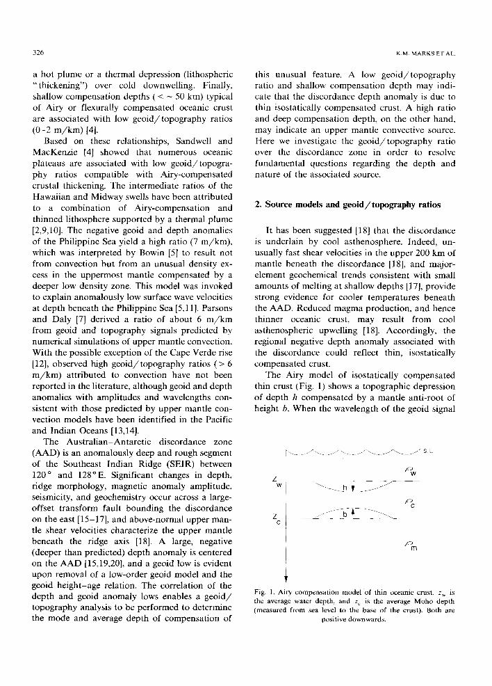
The Airy model of isostatically compensated thin crust (Fig. 1) shows a topographic depression of depth h compensated by a mantle anti-root of height b. When the wavelength of the geoid signal

z W

z O

f ~ W

P G

P r n

Fig. 1. Airy compensation model of thin oceanic crust, z w is the average water depth, and z c is the average Moho depth (measured from sea level to the base of the crust). Both are

positive downwards.

M A N T L E D O W N W E L L I N G B E N E A T H T H E A U S T R A L I A N A N T A R C T I C D I S C O R D A N C E Z O N E 327

TABLE 1

Parameter definitions and values

Param- Definition Value eter

a thermal expansion 3.2 X 10- 5 o C 1 coefficient

g acceleration of gravity 982 cm s 2 G gravitational constant 6.67 x 10- 8

cm3 g-1 s 2 thermal diffusivity 8 × 10 3 cm 2 s- 1

Pw water density 1.03 g cm 3 Ps sediment density 1.90 g cm- 3 Pc crustal density 2.80 g cm 3 Pm upper mantle density 3.30 g cm 3 T m upper mantle temper- 1333 ° C

ature T O seafloor temperature 0 o C

is much greater than the compensa t ion depth, the geoid anoma ly p red ic ted for this mode l [2] is:

h (,ore -- Pw) ] N= 2 rGg (Pc-Pw) h Zc-Zw

(1) where G is the grav i ta t iona l constant , g is the accelera t ion of gravity, and Pw, Pc, Pm are the densi t ies of seawater , crust, and mantle , respec- t ively (pa ramete r values are given in Table 1). The average water and M o h o depths (away from the anoma lous A A D ) are deno ted z w and z c, respectively. The second te rm in eqn. 1 shows that the square of the t opography cont r ibutes to the pre- d ic ted geoid signal (Fig. 2, dashed curve). This con t r ibu t ion is small , however, and is not evident in the observed g e o i d / t o p o g r a p h y ratios. We therefore l inearize eqn. 1 by taking the average ra t io over the topograph ic range:

AN 2~rG , [ hmax (Pm- Pw) ]

(2) where h ma x is the m a x i m u m dep th of the topographic depress ion. F o r the d i scordance dep th anomaly , we set h ma × = - 1 km (a depress ion is negat ive t opography on the seafloor), Zw = 4.2 km, and z c = 10.2 km. Then the g e o i d / t opog raphy ra t io p red ic ted by eqn. 2 for compensa ted thin oceanic crust is 0.4 m / k m .

Ano the r poss ib le source of the d i scordance is some type of upper mant le downwel l ing process.

0 AIRY T H_I N..CRUST

. . . . . . . . . . . THERMAL DEPRESSION Zm = 34 km

~.-I

I Q

L~ 2

-3 L -2 -I

TOPOGRAPHY (km)

Fig. 2. Oeoid height versus topography from the thin crust and thermal depression models. The predicted slopes are _< 0.4 m/kin for the Airy thin crust model and 2.7 m/km for the convectively maintained thermal depression model, z m is de-

fined in Fig. 3.

Hayes [19] suggested that the downwel l ing l imbs of two upper mant le convec t ion cells are converging benea th the d i scordance zone. Indeed, an analysis of gravi ty and dep th anomal ies over the discordance [20] shows high coherences and low phase lags in the 350-500 k m wavelength band , a resul t cons is tent with numer ica l mode l s of uppe r mant le convect ion. A n a l ternat ive bu t s imilar exp lana t ion p roposed by Vogt and Johnson [21] is that as thenospher ic flows f rom the A m s t e r d a m ho t spo t to the west, and the Bal leny and T a s m a n t i d hotspots to the east, are f lowing down grad ien t towards the deep d i scordance zone, u l t imate ly col- l iding there. H o t s p o t - p r o d u c e d flows app roach ing the d i scordance f rom the east are s t rongly indi- ca ted because lavas f rom p r o p a g a t i n g rifts east of the A A D are geochemica l ly ident ica l to those f rom p ropaga t i ng rifts associa ted with ho t spo ts [22]. In addi t ion , as thenosphere f lowing wes tward a long the r idge axis appears to be res t r ic ted by the large-offset ( > 100 km) t r ans fo rm fault b o u n d i n g the d i scordance on the east [23,24]. The corre la- t ion of geoid and dep th a noma ly lows over the A A D is cons is ten t wi th the downwel l ing of these flows.

In ei ther case, downwel l ing as thenosphere will be associa ted with a higher g e o i d / t o p o g r a p h y ra t io and greater c ompe nsa t i on d e p t h than is pre- d ic ted for i sos ta t ica l ly c o m p e n s a t e d thin oceanic crust. Parsons and Da ly [7] c o m p u t e d a geoid

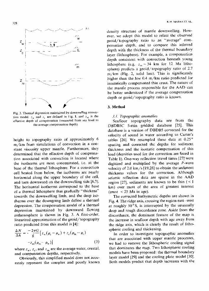
328

z W

z C

~ _ ~ ~ ~ ~ SL.

W

f > C

m

ffl ~ _ j

I

Fig. 3. Thermal depression maintained by downwelling convection model, zw and z c are defined in Fig. 1, and Zm is the effective depth of compensation (measured from sea level to

the average compensation depth).

height to topography ratio of approximately 6 m / k m from simulations of convection in a constant viscosity upper mantle. Furthermore, they determined that the effective depth of compensation associated with convection is located where the isotherms are most concentrated, i.e. at the base of the thermal lithosphere. For a convection cell heated from below, the isotherms are nearly horizontal along the upper boundary of the cell, and turn downward on the downwelling side [6,7]. The horizontal isotherms correspond to the base of a thermal lithosphere that gradually "thickens" towards the downwelling limb, and the deep isotherms over the downgoing limb define a thermal depression. The compensation model of a thermal depression maintained by downward flowing asthenosphere is shown in Fig. 3. A first-order, linearized approximation of the geo id / topography ratio predicted from this model is [4]:

A N _ - 2 q T G [ Z w ( P c _ P w ) --k Z c ( P m -- Pc) Ah g

- z . , ( P . , - Pw)] (3)

where z w, z c, and z m are the average water, crustal, and compensation depths, respectively.

Obviously, this simplified model does not accu- rately represent the complex and poorly known

K.M. MARKS ET AL.

density structure of mantle downwelling. How- ever, we adopt this model to relate the observed geo id / topography ratio to an "average" compensation depth, and to compare this inferred depth with the thickness of the thermal boundary layer (lithosphere). For example, a compensation depth consistent with convection beneath young lithosphere (e.g. z m - 34 km for 12 Ma lithosphere) predicts a geo id / topography ratio of 2.7 m / k m (Fig. 2, solid line). This is significantly higher than the low 0.4 m / k i n ratio predicted for isostatically compensated thin crust. The nature of the mantle process responsible for the AAD can be better understood if the average compensation depth or geo id / topography ratio is known.

3. Method

3.1. Topographic anomalies Seafloor topography da ta are f rom the

DBDB5C 5-min gridded database [25]. This database is a version of DBDB5 corrected for the velocity of sound in water according to Carter 's tables [26]. We resampled these data at 0.25 ° spacing and corrected the depths for sediment thickness and the isostatic compensation of this load (densities used for the correction are listed in Table 1). One-way reflection travel times [27] were digitized and multiplied by the average P-wave velocity of 2.0 k m / s [19,28] to obtain the sediment thickness values for the correction. Although seismic reflection data are sparse in the A A D region [27], sediments are known to be thin ( < 1 km) over most of the area of greatest interest (crust < 25 Ma in age).

The corrected bathymetric depths are shown in Fig. 4. The ridge axis, crossing the region east-west at roughly 50°S, is interrupted by the unusually deep and rough discordance zone. Aside from the discordance, the dominant feature of the map is the increase in seafloor depth with age away from the ridge axis, which is clearly the result of lithospheric cooling and thickening.

In order to investigate topographic anomalies that are associated with upper mantle processes, we had to remove the lithospheric cooling signal that dominates the map. Two lithospheric cooling models have been proposed: the thermal boundary layer model [29] and the cooling plate model [30]. Both models predict that depth increases with the


4 0 $

5 0

6 0 S

110 E 1 2 0 1 3 0 1 4 0 E

C.I. 4.00 m

Fig. 4. DBDB5C topographic data corrected for sediment loading. The heavy line is the ridge axis, thin lines are 15 and

30 Ma crustal isochrons.

square root of age for seafloor 60 Ma and younger. For older seafloor, the depths continue to increase for the thermal boundary layer model, whereas those predicted by the cooling plate model tend to flatten and reach a constant value. The study area covers seafloor approximately 40 Ma and younger, so either model may be used. The depth-age relation used in this study is that of the thermal boundary layer model:

D ( t ) = Do + Ct 1/2 (4) where t is the age, D(t) is the predicted depth, and D o is the depth at which the crust was formed. The subsidence constant, C, is:

2 PmaTm 1/2

where a is the thermal expansion coefficient, • is the thermal diffusivity, T m is the upper mantle temperature, and Pw and Pm are the densities of water and mantle, respectively (parameter values are given in Table 1). We chose the D o value of 2700 m and the subsidence constant of 350 m / m . y . 1/2, which Cochran [31] determined best fit the ridge crest depth and normally subsiding ridge flanks east and west of the discordance (with exception of the northern flank east of the AAD, which is subsiding at an unusually high rate).

Depth anomalies are the difference between depths predicted by the dep th -age relation (eqn. 4) and observed depths corrected for sound velocity and sediment loading. Following Menard [32], we define an area deeper than predicted as having a negative depth anomaly.

The ages used in the depth-age relation (eqn. 4) were compiled from three sources. In the vicinity of the discordance, the ages are from crustal isochrons interpreted by Vogt et al. [33] from a detailed aeromagnetic survey [34]. Ages for the remainder of the study area were determined from the magnetic anomaly identifications of Weissel and Hayes [35] and the revised identifications of Cande and Mutter [36]. A grid of ages for the study area was constructed by interpolating along longitude bands, a method appropriate for an east-west trending ridge axis.

Depth anomalies remaining after removal of the lithospheric cooling signal are due to crustal and upper mantle sources and flexure of the lithosphere. The depth data were high-cut filtered at 400 km so as to eliminate the shorter wavelength flexural and crustal signals. The filter design is the same as that for geoid filtering, and is discussed in the following section. Whereas very long-wavelength geoid anomalies ( > 4000 km) are explained by deep-seated density variations [8,38], a similar origin for comparable topographic anomalies does not apply [38]. Instead, in regions not influenced by subduction, long wavelength topography anomalies primarily reflect cooling of the lithosphere. The topography data are therefore effec- tively band-pass filtered by subtraction of the depth-age relation (assuming the correct lithospheric cooling signal is used) and high-cut filtering. These band-passed residual topography data are shown in Fig. 5, and are used in the geo id / topography analysis.

3.2. Geoid anomalies The raw 1 /8 ° gridded geoid height data used

in this study are those computed by Marsh et al. from SEASAT altimeter data (Marsh, pers. com- mun., 1988). The data were resampled at 0.25 ° spacing, and are shown in Fig. 6 referenced to the GRS80 ellipsoid [39]. The geoid data are domi- nated by an unusual long-wavelength saddle centered on the discordance. Bowin [38] suggested that long wavelength ( > 4000 km) geoid anoma-

330 K.M. MARKS ET AL.

4 0 S

50'

6 0 S

1 1 0 E 1 2 0 1 3 0 1 4 0 E

C . I 200 m

Fig. 5. Residual depth anomalies are DBDB5C topography data corrected for age, sediment loading, and high-cut filtered to remove wavelengths < 400 km. Depth anomalies deeper than - 6 0 0 m are shaded. The heavy line is the ridge axis, dashed fines are fracture zones, and thin solid lines are 15 and

30 Ma crustal isochrons.

lies are due to mass anomalies in the lower mantle and topography on the core mantle interface. Be- cause we are interested in intermediate wavelength (400-4000 km) geoid anomalies arising from density variations in the upper mantle, it is desirable

5O

, o

1 1 0 E 1 2 0 130 140 E

C,I. 2m

Fig. 6. Observed SEASAT geoid heights referenced to the GRS80 ellipsoid.

to remove the regional geoid field due to these deep seated density variations from the raw data.

Geoid model PGSS4 [40] to degree and order 10 represents the regional geoid field arising from mass anomalies deep in the earth. Upon subtraction of this low-order geoid model from the raw geoid height data, residual geoid anomalies pro- duced by mass anomalies in the earth's crust and upper mantle remain. The method commonly used to compute low-order geoid models is to expand the spherical harmonic coefficients to a specific degree and order (usually 10 or 12). The coefficients are simply truncated at the highest harmonic degree. Recently, however, Sandwell and Renkin [10] verified that ringing (i.e. the Gibbs effect) is introduced into the residual geoid anomalies by subtracting a truncated low-order geoid model from the raw data. To eliminate the spurious ringing, they suggest smoothly rolling off the spherical harmonic coefficients around the cut-off degree. A Gaussian function to taper the coefficients between degrees 2 and 25 was used in their analysis. Following their example, we tapered the PGSS4 harmonic coefficients, but selected a one- sided Hanning cosine bell function [41], and rolled off the coefficients between degrees 8 and 15. The study area, 3 8 ° - 6 0 ° S and 105° -140°E , covers a region approximately 2450 km by 2550 km. De- gree 15 corresponds to a 2670 km wavelength, which is larger than the study area. Thus geoid anomalies with wavelengths the size of the study area and smaller are not attenuated when the regional geoid computed with the Hanning taper is subtracted, whereas the Gaussian function would attenuate anomalies within the study area. The cosine tapering function is:

w(/) w(/)

= l l < 8

= 0.5 -t- 0 .5 COS[ q'T()Xma x -- 2~rRc/l )

/ ( X m a x - ~kmin)] 8 > / ~ 1 5

= 0 l > 1 5

(6)

w(t) where w(l) is the weight, l is the degree, R e is the radius of the earth, ~max = 4900 km ( 1 - 8 ) , and )t,nin =2600 km ( l - 1 5 ) . The harmonic coefficients are multiplied by the weights prior to sum- ming the expansion series.

Residual geoid anomalies resulting from the removal of the low-order model from the raw data are shown in Fig. 7. The long-wavelength saddle

M A N T L E D O W N W E L L I N G B E N E A T H T H E A U S T R A L I A N - A N T A R C T I C D I S C O R D A N C E Z O N E 331

6 0 S - - ' " ' -

1 1 0 E 1 2 0 1 3 0 1 4 0 E

C.I. l m

Fig. 7. Geoid heights remaining after a low-order geoid model (PGSS4) is subtracted from the observed geoid heights.

that dominates the raw geoid has been removed with the low-order model. The dominant feature of the residual geoid anomaly map is instead an east-west trending high that correlates with the location of the ridge axis. The geoid high de- creases with distance from the ridge axis and becomes negative on both flanks of the SEIR. Superimposed on the ridge high is a relative low, circular in shape, that is centered on the discordance. It is the correlation of this geoid low with the negative depth anomaly that permits the following geoid/ topography analysis.

The decrease in residual geoid height away from the ridge axis is roughly linear with increas- ing age of the oceanic crust. This indicates that the low-order geoid model did not remove the geoid signal associated with lithospheric cooling, or at least not wavelength components of the lithospheric signal smaller than the size of the study area. Figure 8 shows the residual geoid heights plotted against age of the oceanic crust. The least squares slope of the geoid height-age data is -0 .133 m/m.y . This agrees remarkably well with the slope -0 .131 +0.041 m/m.y , computed by Sandwell and Schubert [42] for a portion of the Southeast Indian Ocean that includes the study area. They obtained this geoid height-age slope by taking the dot product of the horizontal gradient of geoid height and the horizontal gradient of

crustal age. Thus the slope of the geoid height-age data that remains after removal of the low-order geoid model is virtually identical to that computed directly from the raw data. This confirms that the geoid signal due to lithospheric cooling was not removed along with the regional field. For anomalies of upper mantle origin to be isolated, a geoid height-age relation must be explicitly removed from the residual geoid anomalies.

It has been reported in the literature that long wavelength geoid anomalies associated with plate cooling are, to an extent, removed twice when both a low-order geoid model and the geoid height-age relation are subtracted from raw geoid data (e.g. Jung and Rabinowitz, [43]), and Sand- well and Renkin [10] have cautioned against this practice. Over old oceanic crust (> 60-80 Ma), where the geoid height-age relation may flatten and more closely match the behavior predicted by the cooling plate model, the geoid signal due to cooling is predominately long wavelength and its removal, along with a low-order geoid, constitutes a double correction. However for an area comprising younger seafloor (< 60 Ma), and in particular an intermediate or slow spreading mid-ocean ridge, the geoid height-age relation is not flat. Rather, it has a slope consistent with that predicted by the thermal boundary layer model of lithospheric cooling [2], and therefore contains short and intermediate wavelength components. Thus the subtraction of both a low-order geoid and the geoid

6

4

2 ~ . . . , j . • .

. : •

v • • •

" - L " - ° • -~-2F , ,4=' l r<~t,~. •

I " - -'F ": "" "

t ' -6 •

-8 L L , x ,

0 10 20 30 40

A G E (m. y . )

Fig.

5O

8. Low-order corrected geoid heights plotted against age. Least squares line has a -0 .133 m/m.y , slope.


height-age relation over a region of young seafloor does not remove the age effect twice.

A theoretical relationship between geoid height and crustal age has been derived by Haxby and Turcotte [2] for the thermal boundary layer model:

N = -- [ 2 P m @ ( T m - T O ) ] -2qrGPm°~(Tm To)}; I + t

g

(7)

- 2 ~ r G p m a ( T ~ - T0)}; t (8) g

where N is the geoid height, c~ is the thermal expansion coefficient, (T m - To) is the temperature difference across the thermal boundary layer, K is the thermal diffusivity, Pm is the density of the mantle, Pw is the density of water, and t is the age of the lithosphere. The second term in eqn. 7 is negligible [2], and eqn. 8 clearly shows the linear relationship between geoid height and crustal age. The slope of the geoid height-age relation depends on the thermal parameters of the oceanic lithosphere c~, (T m - T o ) , and };, and the mantle density 0.1.

To be consistent, we have used the same parameters to calculate the slope of the geoid height-age relation as were used in the subsidence constant of the dep th -age relation (see Table 1). Substituting these values into eqn. 8 we obtain a geoid height-age slope of -0 .152 m / m . y . It is this slope that we subtract from the residual geoid anomalies to correct for the effect of the cooling lithospheric plate. The low -0 .133 m / m . y , slope determined from the observed geoid height-age data is a result of lithospheric thermal a n d / o r mantle density parameters that deviate from those generally accepted as normal. An unusual upper mantle process beneath the discordance may be responsible for the atypical parameters, as well as other anomalous features associated with the A A D [24].

Upon removal of the low-order geoid and the geoid height-age relation from the raw data, only signals caused by mass anomalies in the crust and upper mantle of the earth remain. Our interest, however, is in the depth of compensation of the discordance zone, and the nature of any associated upper mantle process. To further isolate the signals of interest, we filtered the geoid height data to remove wavelengths _< 400 kin, thereby

40 S

50

60S 110 E 120 130 140 E

C.I. 04m Fig. 9, Res idua l geoid anomal ies are f rom observed S E A S A T geoid heights corrected for a low-order geoid, age, and high-cut

filtered. Geo id anomal ies < 2.4 m are shaded. The heavy l ine is the r idge axis, dashed l ines are f rac ture zones, and thin solid

l ines are 15 and 30 M a crus ta l isochrons.

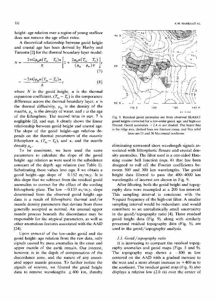
eliminating unwanted short wavelength signals associated with lithospheric flexure and crustal density anomalies. The filter used is a one-sided Han- ning cosine bell function (eqn. 6) that has been designed to roll off the Fourier coefficients between 500 and 300 km wavelengths. The geoid height data filtered to pass the 400-4000 km wavelengths of interest are shown in Fig. 9.

After filtering, both the geoid height and topography data were resampled at a 200 km interval. This sampling interval is consistent with the Nyquist frequency of the high-cut filter. A smaller sampling interval would be redundant, and would contribute to an unrealistically small uncertainty in the geo id / topography ratio [4]. These residual geoid height data (Fig. 9), along with similarly processed residual topography data (Fig. 5), are used in the geo id / topography analysis.

3.3. G e o i d / t o p o g r a p h y ra t i o

It is interesting to compare the residual topography anomalies and geoid maps (Figs. 5 and 9). The topography map shows a - 8 0 0 m low centered on the AAD with a gradual increase to the west and a more abrupt increase to + 400 m to the southeast. The residual geoid map (Fig. 9) also displays a relative low (2.0 m) over the center of

MANTLE DOWNWELLING BENEATH THE AUSTRALIAN ANTARCTIC DISCORDANCE ZONE 333

the AAD with a sharp increase to greater than 4 m toward the southeast. This east to west trend is little influenced by errors in the nor th-south gradients associated with age effects that have been removed from the geoid height and topography data and consequently dominates the quanti- tative geoid height versus topography analysis described below.

The ratio of geoid height to topography as a function of wavelength (the geoid/ topography transfer function) has been determined for Airy and thermal compensation models [10]. Sandwell and Renkin [10] showed that both transfer functions are relatively flat (i.e. the ratio is constant) between - 6 0 0 and 4000 km wavelengths, and depend only on the compensation depth. Based on these properties, they concluded that the observed ratio of appropriately band-pass filtered geoid and topography data could be analyzed in the space domain. This enables the average compensation depth of irregularly shaped areas to be determined, and is useful here for analyzing regions delineated by isochrons (see next section).

The geoid/ topography ratio is obtained by plotting the residual geoid heights (Fig. 9) against residual topography (Fig. 5), and calculating the slope of the best fit line. Traditionally, this is accomplished using the technique of linear regression, where geoid height is regressed on topography. The assumption made is that the topography data are uncertainty-free and the geoid height data are not, i.e. the x-axis (topography) is independent and the y-axis (geoid height) is dependent. Thus the line minimizes the sum of the squares of the geoid height residuals.

Considering that we are utilizing databases that have been gridded from irregular and widely spaced ship tracks in the case of topography, and satellite passes that are very dense along-track yet widely spaced ( - 70 km at 50 o S) between passes in the case of geoid height, we need not assume that all the uncertainties are contained in the geoid height data. It is more appropriate to assume that uncertainties are present in both data sets. However, the misfits between the straight line and the data points are much greater than the errors in either the geoid or topography measure- ments. Thus, we believe that the misfits represent random departures from the compensation models, or even inadequacies in the models, and to a

smaller extent, the measurement errors. Under these conditions, the best fit line is obtained from functional analysis (i.e., non-biased linear regression), where the straight line minimizes both geoid height and topography residuals [44]. The best line thus minimizes the sum:

E , [ w ( X , l ( x , - X i ) ~ + w ( g ) ( y , - ~)2] (9) where X,, Y, are the topography and geoid height observations, xi, y, are points on the best line y~ = a + bx i, and w(X,), w(Yi) are the weights assigned to the observations [45].

Although it is clear that uncertainties are present in both data sets, the amount of uncertainty is not known, because it largely reflects random variations or even inadequacies in the models. We cannot therefore determine weights for w(X,) and w(Y~). However, we can consider the ratio w(Xi)/w(Yi) , and make the reasonable assumption that the ratio equals a constant, c. The slope (b) of the best line is then:

2 2 1 1 / 2 ~

/2Sxy (10)

where Sxx = Ei(Xi - ( X ) ) 2, S~y = E i ( ~ - ( y ) )2 , S x y = Z i ( x i - ( x ) ) ( Y , - ( Y ) ) , and the terms in brackets are the mean values [45]. The difficulty arises in the estimation of c. Much has been written on the subject of estimating c (e.g. Mark and Church, [44]; Jones, [45]), however for our problem where the uncertainties are unknown, the best estimate is obtained when w(Y,) = 1/S,y and w ( ~ ) = 1/Sxx [45]. Inserting this ratio into eqn. 10, the slope (b) reduces to a simple form:

b = + ( s . / s x x ) 1/2

where the correct sign is obtained from Sxy. This best line is called the "reduced major axis" [45]. We obtained the geoid / topography ratio from the slope of this best fit line. We define the error in the slope of the reduced major axis as the difference between the slope of the line that minimizes only geoid height residuals (the traditional least squares method) and the slope of the line that minimizes only topography residuals (also the traditional method, but with the x-axis the dependent variable), divided by the slope of the reduced


major axis. The improvement of the line fit by functional analysis is demonstrated in Figs. l l a - c .

4. Results and discussion

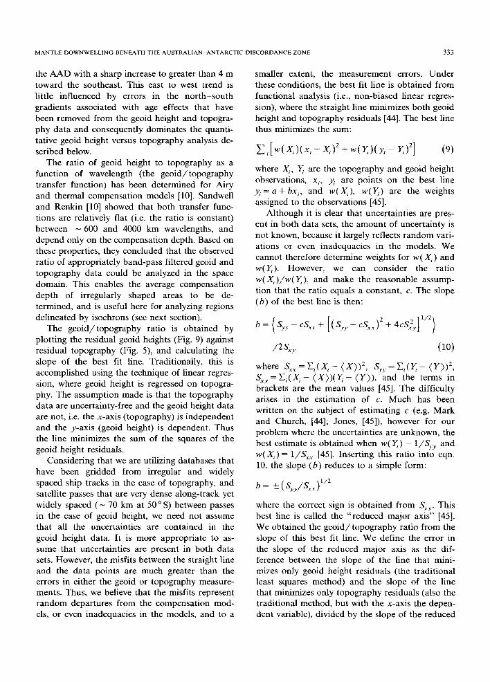
Assuming local isostatic compensation, the ratio of geoid height to topography in the 400-4000 km wavelength band depends on the average compensation depth. The observed ratios may therefore be used to estimate the depth to compensation in the discordance area. The depth determined, however, is also an average depth for the spatial area considered. In order to crudely outline variations in compensation depth over the region, we performed the geo id / topography analysis for the entire study area, a subset comprising crust _< 25 Ma, and a smaller area centered on the AAD. These three regions are delineated in Fig. 10.

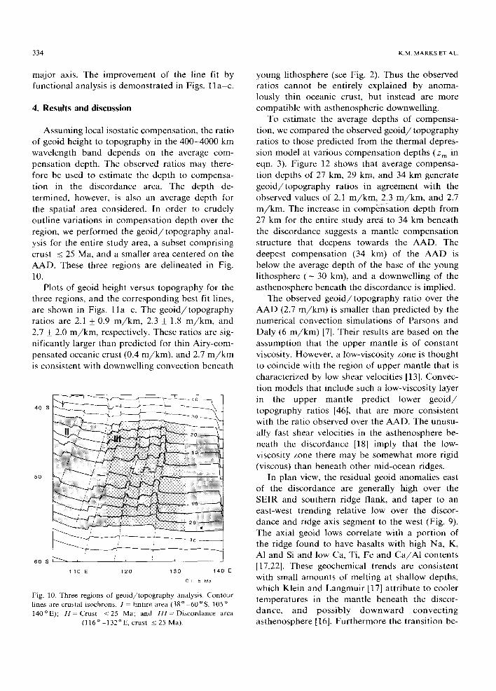
Plots of geoid height versus topography for the three regions, and the corresponding best fit lines, are shown in Figs. l l a c. The geo id / topography ratios are 2.1 _+ 0.9 m / k m , 2.3 _+ 1.8 m / k m , and 2.7 _+ 2.0 m / k m , respectively. These ratios are significantly larger than predicted for thin Airy-compensated oceanic crust (0.4 m / k m ) , and 2.7 m / k m is consistent with downwelling convection beneath

4 0 S

50

6 0 8

1 10 E 1 2 0 1 3 0 1 4 0 E

C . I 5 Ma

Fig. 10. Three reg ions o f g e o i d / t o p o g r a p h y analys is . C o n t o u r lines a re c rus ta l i sochrons . 1 - Ent i re a rea (38 o 60 o S, 105 o

140 ° E ) ; I I - C r u s t _< 25 Ma; a n d I l l ~ D i s c o r d a n c e a rea

( 1 1 6 ° - 1 3 2 ° E , c rus t _< 25 Ma) .

young lithosphere (see Fig. 2). Thus the observed ratios cannot be entirely explained by anomalously thin oceanic crust, but instead are more compatible with asthenospheric downwelling.

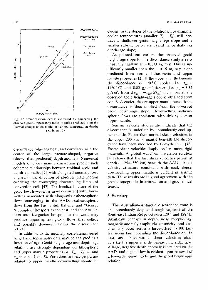
To estimate the average depths of compensation, we compared the observed geo id / topography ratios to those predicted from the thermal depression model at various compensation depths (z m in eqn. 3). Figure 12 shows that average compensation depths of 27 km, 29 kin, and 34 km generate geo id / topography ratios in agreement with the observed values of 2.1 m/k in , 2.3 m/k in , and 2.7 m / k m . The increase in compensation depth from 27 km for the entire study area to 34 km beneath the discordance suggests a mantle compensation structure that deepens towards the AAD. The deepest compensation (34 km) of the A A D is below the average depth of the base of the young lithosphere ( - 30 km), and a downwelling of the asthenosphere beneath the discordance is implied.

The observed geo id / topography ratio over the AAD (2.7 m / k i n ) is smaller than predicted by the numerical convection simulations of Parsons and Daly (6 m / k m ) [7]. Their results are based on the assumption that the upper mantle is of constant viscosity. However, a low-viscosity zone is thought to coincide with the region of upper mantle that is characterized by low shear velocities [13]. Convec- tion models that include such a low-viscosity layer in the upper mantle predict lower geo id / topography ratios [46], that are more consistent with the ratio observed over the AAD. The unusually fast shear velocities in the asthenosphere beneath the discordance [18] imply that the low- viscosity zone there may be somewhat more rigid (viscous) than beneath other mid-ocean ridges.

In plan view, the residual geoid anomalies east of the discordance are generally high over the SEIR and southern ridge flank, and taper to an east-west trending relative low over the discordance and ridge axis segment to the west (Fig. 9). The axial geoid lows correlate with a portion of the ridge found to have basalts with high Na, K, AI and Si and low Ca, Ti, Fe and Ca/A1 contents [17,22]. These geochemical trends are consistent with small amounts of melting at shallow depths, which Klein and Langmuir [17] attribute to cooler temperatures in the mantle beneath the discordance, and possibly downward convect ing asthenosphere [16]. Furthermore the transition be-

M A N T L E D O W N W E L L I N G B E N E A T H T H E A U S T R A L I A N - A N T A R C T I C D I S C O R D A N C E Z O N E 335

4

I-- I

t.l.I 3 I O

ILl (9

2

6 5 I (a)

0 L_

- 2

f •

f /

D •

/7: ,i

-1 0 1

TOPOGRAPHY (kin)

4

f..- I

W 3 "l- r'~

I l l (5

2

6

(b)

5

0 - 2

• "

_ _ i i i

-1 0 1

TOPOGRAPHY (kin) 2

4

F - " r

u.t 3 I 0

U.I (.9

2

6

(c}

5

/ •

, / "

# , , , , re~#~

1

0 i __1 - 2 -1 1

TOPOGRAPHY (kin)

2

Fig. 11. Residual geoid height versus residual topography for the three regions (I, H, and I H ) in Fig. 10. (a) Entire study area, solid line computed from functional analysis, slope = 2.1 m/km; dashed lines are from the traditional least squares method described in text, slopes = 1.4 and 3.3 m/kin. (b) Crust < 25 Ma, slope = 2.3 m/km from functional analysis (solid line), slopes = 1.0 and 5.1 m/km from traditional least squares (dashed lines). (c) Discordance area (116 ° -132°E, crust < 25 Ma), slope = 2.7 m/km from

functional analysis (solid line), slopes = 1.2 and 6.7 from traditional least squares (dashed lines).

t w e e n the ax ia l g e o i d l o w s a n d h i g h s is c o i n c i d e n t w i t h a " m a j o r d i s c o n t i n u i t y in p o s t - m e l t i n g p r o c e s s e s " that d o m i n a t e s the m a j o r - e l e m e n t

c h e m i s t r y a n d is l o c a t e d at the e a s t e r n b o u n d a r y o f the A A D [22].

A 0.5 m geoid low c l o s u r e is c e n t e r e d o n the

3 3 6 K.M. M A R K S ET AL.

OBSERVED RATIO

PREDICTED RATIO Zm = 27 km

Zm - 29 km

Zm - 34 km

/ J 2 2.7 rn/km

2.3 m/kin . / ~

0 i

-1 0

T O P O G R A P H Y ( k m )

Fig. 12. Compensation depths estimated by comparing the observed geoid/topography ratios to ratios predicted from the thermal compensation model at various compensation depths

(z m in eqn. 3).

discordance ridge segment, and correlates with the center of the large, arcuate-shaped, negative (deeper than predicted) depth anomaly. Numerical models of upper mantle convection predict such coherent relationships between residual geoid and depth anomalies [7], with elongated anomaly lows aligned in the direction of absolute plate motion overlying the converging downwelling limbs of convection cells [47]. The localized nature of the geoid low, however, is more consistent with downwelling associated with along-axis asthenospheric flows converging in the AAD. Asthenospheric flows from the Tasmantid, Balleny, and "George V complex" hotspots to the east, and the Amster- dam and Kerguelen hotspots to the west, may produce opposing along-axis flows that collide and possibly downwell within the discordance [21,24].

In addition to the anomaly correlations, geoid height and topography data may be analyzed as a function of age. Geoid height-age and depth age relations are strongly dependent on lithospheric and upper mantle properties (a, T m - To, e¢, and Pm in eqns. 5 and 8). Variations in these properties related to upper mantle downwelling should be

evident in the slopes of the relations. For example, cooler temperatures (smaller T m - T o ) will produce a shallower geoid height-age slope and a smaller subsidence constant (and hence shallower depth-age slope).

As pointed out earlier, the observed geoid height-age slope for the discordance study area is unusually shallow at -0 .133 m/m.y . This is significantly smaller than the -0 .1 6 m/m.y , slope predicted from normal lithospheric and upper mantle properties [2]. If the upper mantle beneath the discordance is 170°C cooler (i.e. T~, 1160°C) and 0.02 g / c m 3 denser (i.e. Pm=3.32 g / c m 3, from Ap m = --pmaATm) than normal, the observed geoid height-age slope is obtained from eqn. 8. A cooler, denser upper mantle beneath the discordance is thus implied from the observed geoid height-age slope. Downwelling asthenospheric flows are consistent with sinking, denser upper mantle.

Seismic velocity studies also indicate that the discordance is underlain by anomalously cool upper mantle. Faster than normal shear velocities in the upper 200 km of mantle beneath the discordance have been modeled by Forsyth et al. [18]. Faster shear velocities imply cooler, more rigid materials. A global waveform inversion solution [48] shows that the fast shear velocities persist at depth ( - 250 550 kin) beneath the AAD. Thus a velocity structure consistent with cool, dense, downwelling upper mantle is evident in seismic data. These results are in good agreement with the geoid / topography interpretation and geochemical trends.

5. Summary

The Australian-Antarctic discordance zone is an anomalously deep and rough segment of the Southeast Indian Ridge between 120 ° and 128 ° E. Significant changes in depth, ridge morphology, magnetic anomaly amplitude, seismicity, and geochemistry occur across a large-offset (> 100 km) transform fault bounding the discordance on the east, and above-normal shear velocities characterize the upper mantle beneath the ridge axis. A large, negative depth anomaly is centered on the AAD, and a geoid low is evident upon removal of a low-order geoid model and the geoid height-age relation.


We performed a geoid/ topography analysis over the discordance zone to determine the mode and depth of compensation of this unusual feature. In order to roughly outline regional variations in compensation depth, we computed these ratios for the entire study area (38 ° -60 o S, 105 o_ 140°E), a subset comprising < 25 Ma oceanic crust, and a smaller area centered on the AAD. Band-pass filtered (400-4000 km) geoid height and topography data were plotted for the three regions, and geoid/ topography ratios were obtained from the slopes of the best fit lines mini- mizing both geoid height and topography devia- tions. Geo id / topography ratios of 2.1 _+ 0.9 m / k m , 2.3 + 1.8 m/km, and 2.7 _+ 2.0 m/km, respectively, were calculated for the three areas. These ratios are significantly larger than predicted for Airy-compensated thin crust (0.4 m/km), indi- cating that the regional discordance depth anomaly is probably not due to anomalously thin crust caused by low magma production rates at the spreading axis. However the 2.7 m / k m ratio over the AAD is consistent with downwelling convection beneath young lithosphere. Estimated average compensation depths of 27, 29, and 34 km, respectively, suggest a mantle structure that deepens towards the AAD. The deepest compensation (34 km) of the AAD is below the average depth of the base of the young lithosphere, and a downwelling of the asthenosphere beneath the discordance is implied.

In plan view, the residual geoid anomalies are generally high over the SEIR east of the discordance, and taper to an east-west trending relative low over the AAD and the ridge segment to the west. The axial geoid lows correlate with a portion of the ridge inferred from major-element geochemical trends to be underlain by cool upper mantle. Furthermore the transition between the axial geoid highs and lows is coincident with a "major discontinuity in post-melting processes" located at the eastern boundary of the AAD [22]. The localized nature of the 0.5 m geoid low centered on the AAD is consistent with downwelling associated with along-axis asthenosphere flows converging in the AAD.

The observed geoid height-age slope is -0 .133 m/m.y , in the discordance region. This is smaller than the -0 .16 m/m.y , slope predicted for normal lithospheric and upper mantle parameters [2].

An upper mantle that is 170°C cooler and 0.02 g / c m 3 denser than normal can explain the shallow slope, and is consistent with the temperature and density regime implied by fast shear velocities.

Acknowledgments

We thank James G. Marsh for kindly providing tapes of 1 /8 ° by 1 /8 ° gridded Seasat geoid height data. KMM thanks the Naval Research Laboratory for the use of their facilities. Compu- tations were performed at the Allied Geophysical Laboratories, University of Houston.

References

1 S.T. Crough, Thermal origin of mid-plate hot-spot swells, Geophys. J. R. Astron. Soc. 55, 451-469, 1978.

2 W.F. Haxby and D.L. Turcotte, On isostatic geoid anomalies, J. Geophys. Res. 83, 5473-5478, 1978.

3 C.L. Angevine and D.L. Turcotte, Correlation of geoid and depth anomahes over the Agulhas Plateau, Tectonophysics 100, 43-52, 1983.

4 D.T. Sandwell and K.R. MacKenzie, Geoid height versus topography for oceanic plateaus and swells, J. Geophys. Res. 94, 7403-7418, 1989:

5 C. Bowin, Gravity and geoid anomalies of the Philippine Sea: Evidence on the depth of compensat ion for the negative residual water depth anomaly, Mere. Geol. Soc. China 4, 103-119, 1981.

6 D. McKenzie, A. Watts, B. Parsons and M. Roufosse, Planform of mantle convection beneath the Pacific Ocean, Nature 288, 442-446, 1980.

7 B. Parsons and S. Daly, The relationship between surface topography, gravity anomalies, and temperature structure of convection, J. Geophys. Res. 88, 1129-1144, 1983.

8 M.A. Richards and B.H. Hager, Geoid anomalies in a dynamic earth, J. Geophys. Res. 89, 5987-6002, 1984.

9 M. McNutt and L. Shure, Estimating the compensat ion depth of the Hawaiian Swell with linear filters, J. Geophys. Res. 91, 13,915-13,923, 1986.

10 D.T. Sandwell and M.L Renkin, Compensat ion of swells and plateaus in the North Pacific: No direct evidence for mantle convection, J. Geophys. Res. 93, 2775-2783, 1988.

11 L.C. Seekins and T. Teng, Lateral variations in the structure of the Philippine Sea plate, J. Geophys. Res. 82, 317-324, 1977.

12 R.C. Courtney and R.S. White, Anomalous heat flow and geoid across the Cape Verde Rise: Evidence for dynamic support from a thermal plume in the mantle, Geophys. J. R. Astron. Soc. 87, 815-867, 1986.

13 W.F. Haxby and J.K. Weissel, Evidence for small-scale mantle convection from Seasat altimeter data, J. Geophys. Res. 91, 3507-3520, 1986.

14 A. Cazenave, M. Monnereau and D. Gibert, Seasat gravity


undulations in the central Indian Ocean, Phys. Earth Planet. Int. 48, 130-141, 1987.

15 J.K Weissel and D.E. Hayes, The Australian-Antarctic discordance: New results and implications, J. Geophys. Res. 79, 2579-2587, 1974.

16 R.N. Anderson, D.J. Spariosu, J.K. Weissel and D.E. Hayes, The interrelation between variations in magnetic anomaly amplitudes and basalt magnetization and chemistry along the Southeast Indian Ridge, J. Geophys. Res. 85, 3883- 3898, 1980.

17 E.M. Klein and C.H. Langmuir, Global correlations of oceanic ridge basalt chemistry with axial depth and crustal thickness, J. Geophys. Res. 92, 8089-8115, 1987.

18 D.W. Forsyth, R.L. Ehrenbard and S. Chapin, Anomalous upper mantle beneath the Australian-Antarctic discordance, Earth Planet. Sci. Lett. 84, 471-478, 1987.

19 D.E. Hayes, Age-depth relationships and depth anomalies in the southeast Indian Ocean and south Atlantic Ocean, J. Geophys. Res. 93, 2937-2954, 1988.

20 K.M. Marks, P.R. Vogt and S.A. Hall, An analysis of gravity and depth anomalies over the Australian-Antarctic discordance zone (abstract), EOS Trans. AGU 69, 1155, 1988.

21 P.R. Vogt and G.L. Johnson, A longitudinal seismic reflection profile of the Reykjanes Ridge: Part II Implications for the mantle hot spot hypothesis, Earth Planet. Sci. Lett. 18, 49-58, 1973.

22 D.M. Christie, D. Pyle, J.-C. Sempere, J.P. Morgan and A. Shor, Petrologic and tectonic observations in and adjacent to the Australian-Antarctic discordance (abstract), EOS Trans. AGU 69, 1426, 1988.

23 P.R. Vogt, Amplitudes of oceanic magnetic anomalies and the chemistry of oceanic crust: Synthesis and review of 'magnetic telechemistry', Can. J. Earth Sci. 16, 2236-2262, 1979.

24 K.M. Marks, P.R. Vogt and S.A. Hall, Residual depth anomalies and the origin of the Australian-Antarctic discordance zone, in press, J. Geophys. Res., 1990.

25 U.S. Navy Oceanographic Office, Digital bathymetric data base (5-minute), 85-MGG-01, NOAA Geophys. Data Center, Boulder, CO, 1985.

26 D.J.T. Carter, Echo-sounding correction tables, Hydrogr. Dep., Ministry of Defense, U.K., 1980.

27 R.E. Houtz and R.G. MarE, Seismic profiler data between Antarctica and Australia, in: Antarctic Oceanology II, The Australian-New Zealand Sector, D.E. Hayes, ed., Antarct. Res. Ser. 19, pp. 147 164, AGU, Washington, D.C., 1972.

28 R.L. Carlson, A.F. Gangi and K.R. Snow, Empirical reflection travel time versus depth and velocity versus depth functions for the deep-sea sediment column, J. Geophys. Res. 91, 8249-8266, 1986.

29 D.L. Turcotte and E.R. Oxburgh, Convection in a mantle with variable physical properties, J. Geophys. Res. 74, 1458-1474, 1969.

30 D.P. McKenzie, Some remarks on heat flow and gravity anomalies, J. Geophys. Res. 72, 6261-6271, 1967.

31 J.R. Cochran, Variations in subsidence rates along inter-

mediate and fast spreading mid-ocean ridges, Geophys. J. R. Astron. Soc. 87, 421-454, 1986.

32 H.W. Menard, Depth anomalies and the bobbing motion of drifting islands, J. Geophys. Res. 78, 5128-5137, 1973.

33 P.R. Vogt, N.Z. Cherkis and G.A. Morgan, Project Investi- gator-I, Evolution of the Australia-Antarctic discordance deduced from a detailed aeromagnetic study, in: Antarctic Earth Science, R.L. Oliver, P.R. James and J.B. Jago, eds., pp. 608-613, Australian Academy of Science, Canberra, A.C.T., 1983.

34 G.A. Morgan, H.S. Fleming and R.H. Feden, Project Inves- tigator-I, A cooperative US/Australian airborne geomag- netic study south of Australia, in: Proc. 13th Int. Symp. Remote Sens. lII, 1439-1444, 1979.

35 J.K. Weissel and D.E. Hayes, Magnetic anomalies in the southeast Indian Ocean, in: Antarctic Oceanology II, The Australian-New Zealand Sector, D.E. Hayes, ed., Antarct. Res. Ser. 19, AGU, pp. 165-196, AGU, Washington, D.C., 1972.

36 S.C. Cande and J.C. Mutter, A revised identification of the oldest sea-floor spreading anomalies between Australia and Antarctica, Earth Planet. Sci. Lett. 58, 151-160, 1982.

37 B.H. Hager, Subducted slabs and the geoid: Constraints on mantle rheology and flow, J. Geophys. Res. 89, 6003-6015, 1984.

38 C. Bowin, Depth of principal mass anomahes contributing to the earth's geoidal undulations and gravity anomalies, Mar. Geodyn. 7, 61-100, 1983.

39 H. Moritz, Geodetic reference system 1980, Bull. Geodyn. 54, 395-405, 1980.

40 F.J. Lerch, J.G. Marsh, S.M. Klosko and R.G. Williamson, Gravity model improvement for Seasat, J. Geophys. Res. 87, 3281-3296, 1982.

41 E.R. Kanasewich, Time sequence analysis in geophysics, 480 pp., University of Alberta Press, Edmonton, Alia., 1981.

42 D. Sandwell and G. Schubert, Geoid height versus age for symmetric spreading ridges, J. Geophys. Res. 85, 7235- 7241, 1980.

43 W.-Y. Jung and P.D. Rabinowitz, Residual geoid anomalies of the north Atlantic Ocean and their tectonic implications, J. Geophys. Res. 91, 10,383-10,396, 1986.

44 D.M. Mark and M. Church, On the misuse of regression in earth science, Math. Geol. 9, 63-75, 1977.

45 T.A. Jones, Fitting straight lines when both variables are subject to error, I: Maximum likelihood and least-squares estimation, Math. Geol. 11, 1-25, 1979.

46 E.M. Robinson and B. Parsons, Effect of a shallow low- viscosity zone on the formation of midplate swells, J. Geophys. Res. 93, 3144-3156, 1988.

47 F.M. Richter and B. Parsons, On the interaction of two scales of convection in the mantle, J. Geophys. Res. 80, 2529-2541, 1975.

48 J.H. Woodhouse and A.M. Dziewonski, Mapping the upper mantle: Three-dimensional modeling of earth structure by inversion of seismic waveforms, J. Geophys. Res. 89, 5953- 5986, 1984.

mantle downwelling beneath the australian-antarctic

Documents