remote sensing

Article

Comparative Analysis of Summer Upwelling andDownwelling Events in NW Spain:A Model-Observations Approach

Pablo Lorente 1,*, Silvia Piedracoba 2 , Pedro Montero 3, Marcos G. Sotillo 1, María Isabel Ruiz 1

and Enrique Álvarez-Fanjul 1

1 Ports & Coastal Dynamics Division, Puertos del Estado, 28042 Madrid, Spain; marcos@puertos.es (M.G.S.);maribel@puertos.es (M.I.R.); enrique@puertos.es (E.Á.-F.)

2 CETMAR (Centro Tecnológico del Mar), 36208 Vigo, Spain; spiedracoba@cetmar.org3 INTECMAR (Instituto Tecnolóxico para o Control do Medio Mariño de Galicia), 36611 Vilagarcía de Arousa,

Spain; pmontero@intecmar.gal* Correspondence: plorente_externo@puertos.es

Received: 29 June 2020; Accepted: 24 August 2020; Published: 26 August 2020�����������������

Abstract: Upwelling and downwelling processes play a critical role in the connectivity betweenoffshore waters and coastal ecosystems, having relevant implications in terms of intensebiogeochemical activity and global fisheries production. A variety of in situ and remote-sensingnetworks were used in concert with the Iberia–Biscay–Ireland (IBI) circulation forecast system, in orderto investigate two persistent upwelling and downwelling events that occurred in the Northwestern(NW) Iberian coastal system during summer 2014. Special emphasis was placed on quality-controlledsurface currents provided by a high-frequency radar (HFR), since this land-based technology caneffectively monitor the upper layer flow over broad coastal areas in near-real time. The low-frequencyspatiotemporal response of the ocean was explored in terms of wind-induced currents’ structures andimmediacy of reaction. Mean kinetic energy, divergence and vorticity maps were also calculated forupwelling and downwelling favorable events, in order to verify HFR and IBI capabilities, to accuratelyresolve the prevailing surface circulation features, such as the locus of a persistent upwelling maximumin the vicinity of Cape Finisterre. This integrated approach proved to be well-founded to efficientlyportray the three-dimensional characteristics of the NW Iberian coastal upwelling system regardlessof few shortcomings detected in IBI performance, such as the misrepresentation of the most energeticsurface dynamics or the overestimation of the cooling and warming associated with upwelling anddownwelling conditions, respectively. Finally, the variability of the NW Iberian upwelling systemwas characterized by means of the development of a novel ocean-based coastal upwelling index (UI),constructed from HFR-derived hourly surface current observations (UIHFR). The proposed UIHFR

was validated against two traditional UIs for 2014, to assess its credibility. Results suggest that UIHFR

was able to adequately categorize and characterize a wealth of summer upwelling and downwellingevents of diverse length and strength, paving the way for future investigations of the subsequentbiophysical implications.

Keywords: remote sensing; HF radar; upwelling; downwelling; ocean currents; skill assessment;coastal modelling

1. Introduction

Upwelling (UPW) and downwelling (DOW) phenomena represent a key role in the strong physicalconnectivity between offshore waters and coastal ecosystems. Wind-driven coastal UPW has beenextensively studied along the eastern edges of the world’s major ocean basins, as it has relevant

Remote Sens. 2020, 12, 2762; doi:10.3390/rs12172762 www.mdpi.com/journal/remotesensing

Remote Sens. 2020, 12, 2762 2 of 32

implications on biogeochemical activity and global fisheries production [1,2]. Along-shore equatorwardwinds modulate an offshore Ekman transport of surface waters that is compensated by the upliftof oxygen-depleted deep cold waters, injecting nutrients into the near-surface euphotic zone andfostering high marine productivity. UPW episodes commonly last 3–10 days [3,4] and can alternatewith weak-wind periods (relaxation) or even DOW-favorable events where poleward winds induce anet onshore displacement and subduction of surface coastal waters, allowing larvae communities toreach suitable locations and recruit to the shoreline.

Notwithstanding, extremely active and persistent UPW and DOW events can also impactnegatively on coastal ecosystems. During periods of increased offshore advection, some fish andinvertebrate populations are exported from coastal habitats and exhibit reduced recruitment success [5].Equally, an excessive enrichment of surface waters inshore might support the proliferation of harmfulalgal blooms [6]. The opposite-phase circulation patterns during DOW-favorable wind conditions maybe related to the transport and retention of pollutants onto the shoreline, with subsequent biologicaland socioeconomic consequences.

The Galician UPW system (Northwestern (NW) Iberian Peninsula) extends from 42◦ N to 44◦ N(Figure 1). In this region, the seasonality of the ocean dynamics is governed by the relative strengths andlatitudinal shifts of the Azores high-pressure and the Iceland low-pressure systems, defining two largelywind-driven oceanographic seasons. The UPW is predominantly a spring–summer phenomenonthat is dominated by northerly winds and a prevailing south-westward surface flow. Nevertheless,some out of the season UPW episodes have also been reported in autumn or winter [7]. During therest of the year, southerly winds prevail which favor DOW events and the subsequent circulation of anarrow surface poleward flow along the NW Iberian shelf edge, the so-called Iberian Poleward Current(IPC) [8].

The UPW intensity in this region has been shown to be strongly dependent on the wind patternand spatially non-uniform, increasing from the north to the south along the coast [9]. The complexityof the wind field in Galicia is partially associated with the jagged shoreline where Cape Finisterre (CF,denoted in Figure 1b) marks an abrupt change between the zonal north and the meridional west coastsof Galicia. Capes and coastal promontories can modulate UPW processes by inducing important windstress variations and zones of retention [6]. In this context, CF has been documented to act frequentlyas the locus of a persistent and localized UPW maximum and recurrent UPW filaments [10]. UPW tothe north of CF is also present but generally discontinuous in time, remaining distant from the coastand near the edge of the continental shelf [11]. By contrast, south of CF, UPW episodes are morefrequent, intense and generally closer to the coast [12].

The Galician coastal UPW system, albeit profusely investigated, has been mostly described interms of recurrent patterns and the related spatiotemporal variability of diverse met-ocean parameters(e.g., wind, sea surface temperature, salinity, chlorophyll or silicate, among others) by using data fromin situ observational networks, satellite missions or modelling tools [10–15]. Growing considerationhas been recently given to the landward extension of coastal UPW into the NW Iberian semi-enclosedbays [16–19].

However, in the present work, notable emphasis is placed on the sea surface current estimationsprovided by a high-frequency radar (HFR) installed on the Galician shoreline [20–22]. Previousinitiatives have successfully addressed the characterization of UPW, relaxation and DOW events inother regions, worldwide, by using this consolidated land-based technology, since it is able to effectivelymonitor the upper layer flow over broad coastal areas in near-real time. The onset, intensity, durationand variability of such coastal phenomena, along with the associated wind-induced circulation andthe ecological response, can be featured thanks to the high spatial resolution of HFR-derived surfacecurrent maps [23–29]. Additionally, this cutting-edge technology presents a wide range of practicalapplications, encompassing search-and-rescue emergencies, accidental spillages of pollutants, harbormanagement or the skill assessment of ocean numerical models [30,31].

Remote Sens. 2020, 12, 2762 3 of 32

Remote Sens. 2020, 12, x FOR PEER REVIEW 3 of 32

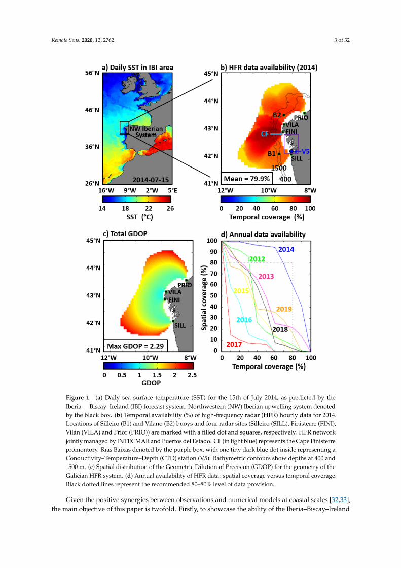
Figure 1. (a) Daily sea surface temperature (SST) for the 15th of July 2014, as predicted by the Iberia––Biscay–Ireland (IBI) forecast system. Northwestern (NW) Iberian upwelling system denoted by the black box. (b) Temporal availability (%) of high-frequency radar (HFR) hourly data for 2014. Locations of Silleiro (B1) and Vilano (B2) buoys and four radar sites (Silleiro (SILL), Finisterre (FINI), Vilán (VILA) and Prior (PRIO)) are marked with a filled dot and squares, respectively. HFR network jointly managed by INTECMAR and Puertos del Estado. CF (in light blue) represents the Cape Finisterre promontory. Rías Baixas denoted by the purple box, with one tiny dark blue dot inside representing a Conductivity–Temperature–Depth (CTD) station (V5). Bathymetric contours show depths at 400 and 1500 m. (c) Spatial distribution of the Geometric Dilution of Precision (GDOP) for the geometry of the Galician HFR system. (d) Annual availability of HFR data: spatial coverage versus temporal coverage. Black dotted lines represent the recommended 80–80% level of data provision.

Figure 1. (a) Daily sea surface temperature (SST) for the 15th of July 2014, as predicted by theIberia—-Biscay–Ireland (IBI) forecast system. Northwestern (NW) Iberian upwelling system denotedby the black box. (b) Temporal availability (%) of high-frequency radar (HFR) hourly data for 2014.Locations of Silleiro (B1) and Vilano (B2) buoys and four radar sites (Silleiro (SILL), Finisterre (FINI),Vilán (VILA) and Prior (PRIO)) are marked with a filled dot and squares, respectively. HFR networkjointly managed by INTECMAR and Puertos del Estado. CF (in light blue) represents the Cape Finisterrepromontory. Rías Baixas denoted by the purple box, with one tiny dark blue dot inside representing aConductivity–Temperature–Depth (CTD) station (V5). Bathymetric contours show depths at 400 and1500 m. (c) Spatial distribution of the Geometric Dilution of Precision (GDOP) for the geometry of theGalician HFR system. (d) Annual availability of HFR data: spatial coverage versus temporal coverage.Black dotted lines represent the recommended 80–80% level of data provision.

Given the positive synergies between observations and numerical models at coastal scales [32,33],the main objective of this paper is twofold. Firstly, to showcase the ability of the Iberia–Biscay–Ireland

Remote Sens. 2020, 12, 2762 4 of 32

(IBI) ocean forecast system [34] (Figure 1a) to adequately reproduce the three-dimensional features oftwo persistent UPW and DOW events during summer 2014 in the NW Iberian Peninsula (Figure 1b).To the extent that UPW and DOW circulation patterns have been previously reported to be recurring [7],their presence also becomes predictable, and thus anticipatory strategies can be efficiently promptedto face environmental affairs such as larval transport pathways or the destination of accidental oilspills [29]. To this end, quality-controlled HFR hourly current estimations, satellite products and insitu observations from buoys and a Conductivity–Temperature–Depth (CTD) device were used inconcert with IBI hydrodynamic model. A thorough characterization of the ocean signatures associatedwith UPW and DOW activities can be achieved thanks to their complementary and interdependentnature. While traditional instrumented platforms provide a close approximation of “ground truth” forremotely sensed estimations, HFR observations enhance numerical simulations by resolving fine-scaleprocesses in intricate regions with complex-geometry configurations. In turn, hydrodynamic modelscan reciprocally serve as integrative connectors of sparse in situ observations and gappy HFR surfacecurrent maps by offering a seamless predictive picture of the three-dimensional ocean state. Secondlyand most importantly, to characterize the variability of the NW Iberian UPW system through thedevelopment of a novel basic ocean-based coastal UPW index, generated from HFR-derived hourlysurface current estimations (UIHFR). Assuming the immediate oceanic response to wind forcing,the proposed high-frequency index can act as a proxy of UPW and DOW conditions. In this context,UIHFR was compared with two preexisting six-hourly UPW indexes for the entire 2014, with thepurpose of evaluating its consistency and variability. Likewise, the ability of UIHFR to categorize UPWand DOW events during summer 2014 was also qualitatively assessed.

This work is structured as follows: Section 2 outlines the observational and modelled datasources, along with the methodology adopted. Results are presented and interpreted in Section 3.A comprehensive discussion and future work are addressed in Section 4. Finally, principal conclusionsare drawn in Section 5.

2. Materials and Methods

2.1. The Galician HFR System

A four-site long-range CODAR SeaSonde network, deployed along the Galician Coast (Figure 1b),was used in this work. The first two sites (owned by Puertos del Estado) were deployed in 2004:Silleiro (SILL) and Finisterre (FINI). Afterward, the network was extended northward, in December2011, by installing two additional sites on phased approach: Vilán (VILA) and Prior (PRIO), ownedby INTECMAR–Xunta de Galicia. Each single radar site operates at a central frequency of 4.86 MHz,with a 29.41 KHz bandwidth, measuring the following:

(i) Hourly radial currents, moving toward or away from the site, that are representative of the upper2 m of the water column. The maximum current speed, horizontal range and angular resolutionare 100 cm·s−1, 200 km and 5◦, respectively. All of those radial current vectors (from two orseveral sites) within a predefined search radius of 25 km are geometrically combined by applyingan unweighted least squares fitting algorithm [35] to estimate hourly total current vectors on aCartesian regular mesh of 6 × 6 km horizontal resolution.

(ii) Thirty-minute wave estimations for five range cells, regularly spaced every 5.1 km, which extendradially from the site. For further details about this dataset, the reader is referred to Reference [22],as the present work is mainly focused on surface circulation.

The hourly data availability during 2014 was significantly high in the center of the domain (above90%), decreasing to 60–70% in the westernmost borders (Figure 1b). The spatially averaged dataavailability was almost 80% for the entire year, revealing that the HFR system performed withinacceptable ranges despite the severe FINI breakdown since November 2014.

The specific geometry of the HFR domain and, hence, the intersection angles of radial vectorshandicap the accuracy of the total current vectors resolved at each grid point. Such a source of

Remote Sens. 2020, 12, 2762 5 of 32

uncertainty is quantified by a dimensionless parameter denominated Geometrical Dilution of Precision(GDOP) [36], which typically increases with the distance from the HFR sites. In this work, a cutoff

filter of 2.3 was imposed for the GDOP, to get rid of those estimations affected by higher uncertainties.Consequently, GDOP values remain below 2 in the core of the spatial domain, reaching maximumvalues of 2.29 at the boundaries of the HFR areal coverage (Figure 1c).

Although this four-site HFR system has been working operationally since 2012, the continueddata provision was dramatically impacted by a number of serious breakdowns, mainly due to severeweather episodes that typically battered the Galician Coast during wintertime. Additionally, the globaleconomic recession also challenged the financial support to preserve the infrastructure core alreadyimplemented. Since the dataset corresponding to 2014 presented both the highest temporal availabilityand maximum areal coverage (Figure 1d), this work was focused on UPW and DOW events occurredduring this specific year.

Finally, note that the present system is part of the cross-border HFR network in the NW of the IberianPeninsula, reinforced in the framework of the RADAR ON RAIA project (Interreg V, a Spain–Portugalcooperative program). This initiative aims at capitalizing oceanographic knowledge through theextension and consolidation of this HFR network and the development of user-oriented products.

2.2. In Situ Buoys

Basic features of two deep ocean buoys, deployed within the HFR footprint (Figure 1b), are gatheredin Table 1. Both in situ devices collect quality-controlled estimations of sea surface temperature (SST),among other physical parameters. Furthermore, since B1 buoy is equipped with an acoustic currentmeter and a wind sensor, it also provides hourly averaged current and wind vectors at 3.5 m depthand 3 m height, respectively.

Table 1. Description of the buoys deployed within HFR coverage.

Buoy Name Model Deployment Longitude Latitude Depth Sampling

B1 Silleiro Seawatch 1998 9.44◦W 42.12◦N 600 m 1 hB2 Vilano Seawatch 1998 9.22◦W 43.50◦N 386 m 1 h

2.3. Upwelling Indexes

Annual (2014) time series of two coastal upwelling indexes (UIs), based on 6-hourly data of sea levelpressure (UIBAIXAS) and wind (UIB1), were used as benchmark in this work to assess the credibility ofthe proposed ocean-based index. Both are freely available at the IEO (Instituto Español de Oceanografía)website: http://www.indicedeafloramiento.ieo.es/index_en.html. UIBAIXAS, which was calculated at42◦N, 10◦W, was derived from the FNMOC (Fleet Numerical Meteorology and Oceanography Center,US Navy) database. UIB1 was computed by using wind data obtained from B1 buoy. For furtherinformation about these two UIs, the reader is referred to Reference [15].

2.4. CTD Device

Water temperature and salinity profiles were measured on a weekly basis, at the inner part of theRías Baixas, using a CTD device (denoted by a purple box and a blue dot, respectively, in Figure 1b),which belongs to a network of 43 oceanographic stations operated by INTECMAR. Since the IBI oceanforecast system is not able to adequately resolve the jagged intricate coastline deep inside the RíasBaixas, only one of the outermost CTD stations was selected to conduct the comparisons: V5 (located at42.18◦N–8.87◦W).

2.5. Satellite-Derived Products

Two daily satellite-derived products, gap-filled and interpolated on a regular grid, were used inthis study, to characterize the UPW and DOW episodes: the first one for the SST (OSTIA: Operational

Remote Sens. 2020, 12, 2762 6 of 32

Sea Surface Temperature and Ice Analysis) and the second one for the chlorophyll (CHL) concentration.Essential features of both products are summarized in Table 2. Additional information can be obtainedin their respective Product User Manuals (PUMs), freely accessible through the Copernicus MarineEnvironment Monitoring Service (CMEMS) catalogue (https://marine.copernicus.eu/)

Table 2. Description of the satellite products used in this work.

Name Variable Type Level Resolution Frequency Provider

OSTIA SST L4 (gap-filled) Surface 0.05◦ Daily UK MetOfficeCHLL4 CHL L4 (gap-filled) Surface 0.01◦ Daily Ocean Color TAC

OSTIA = Operational Sea Surface Temperature and Ice Analysis. CHL = chlorophyll. TAC = ThematicAssembly Center.

2.6. IBI Ocean Forecast System

The CMEMS IBI operational suite consists of a NEMO model v3.6 [37] application, run dailyover a regional grid (Figure 1a) with a horizontal resolution of ∼3 km and 50 unevenly distributedvertical levels. A best estimate of the ocean state (also called “hindcast”) and a five-day-ahead forecastare routinely produced for a number of hydrodynamic variables: temperature, salinity, mixed layerdepth, zonal and meridional velocity currents and sea surface height, among others. While hourlyaveraged estimations are provided at the sea surface, daily averaged values are computed for therest of the three-dimensional water column. The system is driven every 3 h by high-resolution(1/8◦) meteorological forcings provided by the European Center for Medium-Range Weather Forecast(ECMWF). Initial and lateral open-boundary conditions, imposed from daily 3D outputs from theparent system (CMEMS GLOBAL), are complemented with 11 tidal harmonics. The freshwaterdischarges are prescribed through 33 points corresponding to the main rivers present in the IBI area.This version of IBI ocean forecast system does not include an assimilation scheme. For further technicalspecifications, the reader is referred to Reference [38].

2.7. Methods

A battery of basic processing steps was applied to the sea surface temperature, salinity, currentvelocity and wind observations. Given the focus on the low-frequency characteristics of the flow field,any short gap of 6 h or less was filled by applying linear interpolation.

The agreement between two datasets was evaluated by computing a variety of conventionalstatistics: mean (x) and the related standard deviation (σ), mean absolute difference (MAD),root mean squared error (RMSE), scalar correlation, complex correlation (CC) coefficient (ρ) andthe associated phase (θ, in degrees) between two vector fields [39], defined as w1(t) = u1(t) + iv1(t)and w2(t) = u2(t) + iv2(t), among others.

x =1N

N∑i=1

xi (1)

σ =

√√√1

N− 1

N∑i=1

(xi − x)2 (2)

MAD =1N

N∑i=1

∣∣∣xi − yi

∣∣∣ (3)

RMSE =

√√√1N

N∑i=1

(xi − yi

)2(4)

Remote Sens. 2020, 12, 2762 7 of 32

Correlation =1

N− 1

N∑i=1

(xi − xσx

)(yi − yσy

)(5)

ρ =〈u1u2 + v1v2〉√⟨

u21 + v2

1

⟩√〈u1 + v1〉

+ i〈u1u2 − v1v2〉√⟨

u21 + v2

1

⟩√〈u1 + v1〉

(6)

θ = tan−1 〈u1v2 − u2v1〉

〈u1u2 − v1v2〉(7)

HFR estimations were bilinearly interpolated on the finer resolution IBI hindcast mesh, in order toadequately compare both datasets in a common regular domain. The prevailing wind-driven surfacecirculation during UPW and DOW episodes was examined from a Eulerian perspective, by meansof 10-day averaged patterns of surface currents. Complementarily, spatial maps of the CC betweenobserved and modelled current velocity vectors were also calculated, to study their concordanceand infer those areas where the model performance might be more consistent. With the purpose ofbetter understanding the flow dynamics, we estimated a wealth of ancillary diagnostics, such as thehorizontal divergence (DIV), the vorticity (VOR) and the mean kinetic energy (MKE).

DIV =∂u∂x

+∂v∂y

(8)

VOR =∂v∂x−∂u∂y

(9)

MKE =1N

N∑i=1

12

(u2

i + v2i

)(10)

where N, u and v represent the total number of data, the zonal and meridional velocityfields, respectively.

Another method to investigate the flow dynamics and seawater dispersion is the InstantaneousRate of Separation (IROS), which is a Eulerian metric that determines how an infinitesimally smallparticle will be moved by an instantaneous velocity field, and is equal to the finite-time Lyapunovexponent (FTLE) at time t = 0 [40]. This diagnostic, successfully used in previous studies with HFRdata [41,42], can be calculated from the sum of divergence and total strain:

IROS =

(∂u∂x

+∂v∂y

)+

√(∂v∂x

+∂u∂y

)2

+

(∂u∂x−∂v∂y

)2

(11)

While the FTLE unveils a variety of features that dominate over longer time periods, IROS indicateshow the particles react in the selected moment, estimating particle separation from a snapshot withoutintegrating the flow over time. Since IROS does not require time integration, it is a rather simple anduseful diagnostic to examine mean characteristics of the flow in the NW upwelling system. High valuesof IROS indicate potential regions of elevated particle dispersion, which has relevant implications forcross-shelf exchange of passive tracers between offshore and coastal waters.

Finally, a novel ocean-based coastal upwelling index (UIHFR) was developed for the NW Iberianupwelling system. Assuming a direct relationship between atmospheric forcing and the promptresponse of the upper ocean layer, a rather simple index was constructed from HFR-derived hourlyestimations of sea surface currents, spatially averaged over the Galician continental shelf. Similar tothe classical Ekman upwelling index [43], the UIHFR is defined as follows:

UIHFR

(m3·s−1·km−1

)= −

ρA·Cd√

u2 + v2·vf ·ρw

·3× 106 (12)

Remote Sens. 2020, 12, 2762 8 of 32

where ρw is the seawater density (1025 kg·m−3), Cd is a dimensionless empirical drag coefficient(1.4 × 10−3), ρA is the air density in normal conditions (1.22 kg·m−3) and f is the Coriolis parameter.In this case, u and v denote the detided hourly time series of HFR zonal and meridional currentvelocities (m·s−1), respectively. The sign is changed to define positive (negative) magnitudes of UIHFR

as response of the predominant equatorward (poleward) surface flow over the Galician shelf.

3. Results

3.1. Skill Assessment of HFR Estimations

The credibility of HFR-derived current data has been extensively assessed worldwide [44–46] byconducting quantitative comparisons with independent observations provided by in situ platformssuch as drifters, acoustic Doppler current profilers (ADCPs) or current meters (CMs). Routine validationexercises are pertinent since the accuracy of remotely sensed estimations might be negatively affectedby inherent problems of radar technology such as radio frequency interferences, reflections frommoving ships, antenna pattern distortion, adverse environmental conditions or hardware failures,among others [47].

In this context, a preliminary skill assessment of the Galician HFR system was performed for2014. Hourly HFR current estimations at the grid point closest to B1 location were compared withconcurrent observations from a CM installed in B1 (Figure 1b). Comparisons were attempted for boththe zonal and meridional sub-inertial currents, obtained after applying a 10th-order digital low-passButterworth filter with a cutoff period of 30 h [48]. This scheme is adequate, as the study is mainlyconcerned with the low-frequency characteristics of the surface flow.

The visual resemblance between the HFR and CM time series is significantly high for bothcurrent components (Figure 2a,b), with correlation coefficient and RMSE values emerging in theranges (0.53–0.74) and (5.72–8.59) cm·s−1, respectively. These figures are in accordance with similarinvestigations previously conducted in the Iberian waters (Table 3). According to the best linear fitof scatterplots, remote-sensed estimations seem to underestimate, to a small extent, the speed of thesurface currents observed at B1 (Figure 2c,d).

Remote Sens. 2020, 12, x FOR PEER REVIEW 8 of 32

where ρw is the seawater density (1025 kg·m−3), Cd is a dimensionless empirical drag coefficient (1.4 × 10−3), ρA is the air density in normal conditions (1.22 kg·m−3) and f is the Coriolis parameter. In this case, u and v denote the detided hourly time series of HFR zonal and meridional current velocities (m·s−1), respectively. The sign is changed to define positive (negative) magnitudes of UIHFR as response of the predominant equatorward (poleward) surface flow over the Galician shelf.

3. Results

3.1. Skill Assessment of HFR Estimations

The credibility of HFR-derived current data has been extensively assessed worldwide [44–46] by conducting quantitative comparisons with independent observations provided by in situ platforms such as drifters, acoustic Doppler current profilers (ADCPs) or current meters (CMs). Routine validation exercises are pertinent since the accuracy of remotely sensed estimations might be negatively affected by inherent problems of radar technology such as radio frequency interferences, reflections from moving ships, antenna pattern distortion, adverse environmental conditions or hardware failures, among others [47].

In this context, a preliminary skill assessment of the Galician HFR system was performed for 2014. Hourly HFR current estimations at the grid point closest to B1 location were compared with concurrent observations from a CM installed in B1 (Figure 1b). Comparisons were attempted for both the zonal and meridional sub-inertial currents, obtained after applying a 10th-order digital low-pass Butterworth filter with a cutoff period of 30 hours [48]. This scheme is adequate, as the study is mainly concerned with the low-frequency characteristics of the surface flow.

The visual resemblance between the HFR and CM time series is significantly high for both current components (Figure 2a,b), with correlation coefficient and RMSE values emerging in the ranges (0.53–0.74) and (5.72–8.59) cm·s−1, respectively. These figures are in accordance with similar investigations previously conducted in the Iberian waters (Table 3). According to the best linear fit of scatterplots, remote-sensed estimations seem to underestimate, to a small extent, the speed of the surface currents observed at B1 (Figure 2c,d).

Figure 2. Annual (2014) comparison of zonal (a,c) and meridional (b,d) hourly surface current velocities observed by B1 buoy and HFR (at the closest grid point): 30-h low-pass filtered time series (a,b) and best linear fit of scatter plots (c,d). Skill metrics gathered in black boxes.

Figure 2. Annual (2014) comparison of zonal (a,c) and meridional (b,d) hourly surface current velocitiesobserved by B1 buoy and HFR (at the closest grid point): 30-h low-pass filtered time series (a,b) andbest linear fit of scatter plots (c,d). Skill metrics gathered in black boxes.

Remote Sens. 2020, 12, 2762 9 of 32

Table 3. Series of prior studies dealing with the validation of HFR total current vectors against in situobservations in the Iberian waters.

Reference HFR (MHz) Region RMSE/Correlation

[49] CODAR SeaSonde (4.86) Galicia 5–7 cm·s−1/0.68–0.88[50] CODAR SeaSonde (4.53) Bay of Biscay 8–13 cm·s−1/0.34–0.86[51] CODAR SeaSonde (4.53) Bay of Biscay 8–15 cm·s−1/0.27–0.67[52] CODAR SeaSonde (27) Strait of Gibraltar 8–22 cm·s−1/0.31–0.81[53] CODAR SeaSonde (13.5) Ibiza Channel 7–12 cm·s−1/0.59–0.72[20] CODAR SeaSonde (4.86) Galicia 8–13 cm·s−1/0.56–0.74

3.2. Skill of IBI to Reproduce Two Upwelling/Downwelling Events

3.2.1. Selection of Upwelling and Downwelling Events

Although observations at a single point are unlikely to be fully representative of the oceanographicconditions found over the entire study area, hourly wind measured at B1 was low-pass filtered, depictedevery 3 h and later analyzed as a proxy for the local open sea wind regime. An abrupt shift in localwind directions, from July to September 2014, is evidenced in monthly wind roses (Figure 3). Northerlyand northeasterly winds clearly predominated in July (Figure 3a). By contrast, persistent southerly andsoutheasterly winds prevailed during September 2014, with strong gusts up to 12.7 m·s−1 (Figure 3b).Following References [54,55], we identified two anomalously long-lasting UPW and DOW eventsduring summer 2014, by looking at persistently dominant wind directions and sustained high windspeeds above a predefined threshold of 3 m·s−1. The meridional wind regime was permanently directedsouthward and northward, respectively, during 10 consecutive days when no relevant relaxation(below the imposed cutoff) in between was exhibited (Figure 3c,d). Although Reference [56] alreadydocumented the UPW conditions and the resulting coastal dynamics as response to two unusuallypersistent 10-day wind episodes, transient UPW conditions tend to last shorter time [3,4], with anaverage length of ~3 days on the Galician shelf [19].

Remote Sens. 2020, 12, x FOR PEER REVIEW 9 of 32

Table 3. Series of prior studies dealing with the validation of HFR total current vectors against in situ observations in the Iberian waters.

Reference HFR (MHz) Region RMSE/Correlation

[49] CODAR SeaSonde (4.86) Galicia 5–7 cm·s−1/0.68–0.88 [50] CODAR SeaSonde (4.53) Bay of Biscay 8–13 cm·s−1/0.34–0.86 [51] CODAR SeaSonde (4.53) Bay of Biscay 8–15 cm·s−1/0.27–0.67 [52] CODAR SeaSonde (27) Strait of Gibraltar 8–22 cm·s−1/0.31–0.81 [53] CODAR SeaSonde (13.5) Ibiza Channel 7–12 cm·s−1/0.59–0.72 [20] CODAR SeaSonde (4.86) Galicia 8–13 cm·s−1/0.56–0.74

3.2. Skill of IBI to Reproduce Two Upwelling/Downwelling Events

3.2.1. Selection of Upwelling and Downwelling Events

Although observations at a single point are unlikely to be fully representative of the oceanographic conditions found over the entire study area, hourly wind measured at B1 was low-pass filtered, depicted every 3 h and later analyzed as a proxy for the local open sea wind regime. An abrupt shift in local wind directions, from July to September 2014, is evidenced in monthly wind roses (Figure 3). Northerly and northeasterly winds clearly predominated in July (Figure 3a). By contrast, persistent southerly and southeasterly winds prevailed during September 2014, with strong gusts up to 12.7 m·s−1 (Figure 3b). Following References [54,55], we identified two anomalously long-lasting UPW and DOW events during summer 2014, by looking at persistently dominant wind directions and sustained high wind speeds above a predefined threshold of 3 m·s−1. The meridional wind regime was permanently directed southward and northward, respectively, during 10 consecutive days when no relevant relaxation (below the imposed cutoff) in between was exhibited (Figure 3c,d). Although Reference [56] already documented the UPW conditions and the resulting coastal dynamics as response to two unusually persistent 10-day wind episodes, transient UPW conditions tend to last shorter time [3,4], with an average length of ~3 days on the Galician shelf [19].

Figure 3. Wind roses, indicating predominant propagation direction at B1 buoy during July (a) and September (b) of 2014. Stick diagrams (depicted every 3 h) of hourly averaged wind during the 10-day upwelling-favorable (c) and downwelling-favorable events (d).

Figure 3. Wind roses, indicating predominant propagation direction at B1 buoy during July (a) andSeptember (b) of 2014. Stick diagrams (depicted every 3 h) of hourly averaged wind during the 10-dayupwelling-favorable (c) and downwelling-favorable events (d).

Remote Sens. 2020, 12, 2762 10 of 32

3.2.2. Analysis of the Surface Circulation

According to the significant resemblance between observed and modelled mean circulationpatterns, it can be stated that IBI seems to properly resolve the large-scale surface dynamics in the studyarea for both UPW and DOW events (Figure 4). The UPW episode is characterized by a wind-inducedsouthwestward flow, with an offshore advection of coastal waters to the open ocean, in accordancewith Ekman´s theory that postulates a net movement to the right of wind direction in the northernhemisphere (Figure 4a,b). An advective acceleration of surface currents speed over the continentalshelf is revealed in both datasets, especially in the periphery of CF.

Remote Sens. 2020, 12, x FOR PEER REVIEW 10 of 32

3.2.2. Analysis of the Surface Circulation

According to the significant resemblance between observed and modelled mean circulation patterns, it can be stated that IBI seems to properly resolve the large-scale surface dynamics in the study area for both UPW and DOW events (Figure 4). The UPW episode is characterized by a wind-induced southwestward flow, with an offshore advection of coastal waters to the open ocean, in accordance with Ekman´s theory that postulates a net movement to the right of wind direction in the northern hemisphere (Figure 4a,b). An advective acceleration of surface currents speed over the continental shelf is revealed in both datasets, especially in the periphery of CF.

By contrast, a rather uniform poleward surface circulation is evidenced in response to prevailing southerly winds during the DOW episode (Figure 4d,e). On the southern inner shelf, the interplay between the existing topographic barriers and the cross-shore transport led to a marked directional change of the coastal flow to the left, intensified in form of a narrow jet, the well-documented IPC, which circulated along the NW Iberian shelf edge [8,57]. Since river plumes are mainly confined landward during DOW conditions [58], this northward coastal jet apparently was not significantly perturbated by impulsive-type freshwater outflows at this stage of the year.

Figure 4. Ten-day averaged surface circulation patterns during upwelling (UPW, a–c) and downwelling (DOW, d–f) wind-driven events as observed with the high-frequency radar (HFR, a,d) and modelled by IBI ocean forecast system (b,e). The associated complex correlation (CC) index between IBI and HFR is presented (c,f). The isolines show the veering. Bold arrows indicate the predominant propagation direction of the wind registered at B1 buoy (shown in Figure 1b) during the 10-day periods.

Figure 4. Ten-day averaged surface circulation patterns during upwelling (UPW, a–c) and downwelling(DOW, d–f) wind-driven events as observed with the high-frequency radar (HFR, a,d) and modelled byIBI ocean forecast system (b,e). The associated complex correlation (CC) index between IBI and HFRis presented (c,f). The isolines show the veering. Bold arrows indicate the predominant propagationdirection of the wind registered at B1 buoy (shown in Figure 1b) during the 10-day periods.

By contrast, a rather uniform poleward surface circulation is evidenced in response to prevailingsoutherly winds during the DOW episode (Figure 4d,e). On the southern inner shelf, the interplaybetween the existing topographic barriers and the cross-shore transport led to a marked directionalchange of the coastal flow to the left, intensified in form of a narrow jet, the well-documented IPC,which circulated along the NW Iberian shelf edge [8,57]. Since river plumes are mainly confined

Remote Sens. 2020, 12, 2762 11 of 32

landward during DOW conditions [58], this northward coastal jet apparently was not significantlyperturbated by impulsive-type freshwater outflows at this stage of the year.

The primary IBI-HFR disagreement arises from the presence, detached from the coast, of asouthern counter-clockwise eddy-like circulation structure (Figure 4b) and an elongated meander(Figure 4e) in the modelled currents under UPW and DOW conditions, respectively. Conversely,the HFR-derived circulation patterns seem to be more homogeneous, with no proof of the existence ofany coherent vortex (Figure 4a,d).

Maps of CC reflect an overall higher IBI–HFR correspondence in regions close to the shoreline,with the CC index and the related phase lying in the ranges (0.6–0.9) and (0–10◦), respectively, for boththe UPW (Figure 4c) and DOW (Figure 4f) events. These outcomes are in line with earlier worksdealing with the same topic [59,60], where the CC coefficients and the associated (absolute) phaseswere reported to lie between 0.2 and 0.8 and between 0◦ and 20◦, respectively. The degree of accordancetends to decline in areas near the limits of the HFR footprint, where higher GDOP values are indeedencountered, especially within the northernmost sectors (Figure 1c): the CC coefficient drops to(0.2–0.4), and the associated phase increases up to 30◦ (in absolute value) in nearby edges of the HFRdomain (Figure 4c,f). Accordingly, Reference [59] also obtained lower CC coefficients (∼0.4) in remoteareas, distant from the coastline. Spatially averaged skill metrics that were derived from the IBI–HFRcomparison of surface currents for the two selected events are gathered in Table 4. IBI performancewas similar for both episodes, with comparable levels of accuracy for the zonal and meridional currentcomponents. Better statistics were obtained over the continental shelf than in open waters.

Table 4. Overview of skill metrics derived from IBI–HFR comparison of surface currents for the selectedUPW and DOW events, spatially averaged over the entire common domain (Entire) and exclusivelyover the Galician continental shelf (Shelf).

Skill Metric UPW-Entire UPW-Shelf DOW-Entire DOW-Shelf

Zonal RMSE (cm·s−1) 11.00 9.59 11.77 10.48Meridional RMSE (cm·s−1) 10.94 8.26 12.68 11.87

Zonal correlation 0.51 0.61 0.51 0.63Meridional correlation 0.44 0.58 0.42 0.61

CC 0.50 0.63 0.50 0.66

Horizontal divergence at the sea surface was calculated to discriminate zones of contractionand expansion of the flow where vertical flux might be significant in terms of proximal originsand destinations of water particles [27]. Positive surface divergence is generally associated with aconvergence at deeper levels and the subsequent vertical uplift of waters (i.e., UPW). By contrast,regions of negative surface divergence (i.e., convergence) are related to downward motions to lowerlevels (i.e., DOW). Therefore, in order to unveil localized areas of UPW and DOW conditions,maps of horizontal divergence were computed by using both the HFR and IBI datasets (Figure 5).Under UPW-favorable winds, a common peak of positive divergence is exposed in the central portionof the domain (43◦ N of latitude) and also in the periphery of CF, indicating accumulated upwardvertical motions and strong UPW. A large belt of positive coastal divergence, extended from FINIto PRIO radar sites, is exhibited in the HFR dataset (Figure 5a). On the contrary, in the case of IBI,the divergence over the continental shelf seems to be weaker and alternated with areas of horizontalconvergence (Figure 5b). Under dominant southerly winds, strong coastal convergence is evidencednorth of CF, indicating that the surface flow is presumably sinking downward (Figure 5c,d). Both theHFR and IBI maps agree to determine an UPW core around CF (larger and stronger for the latter),confined between two bands of horizontal convergence. This is in agreement with previous historicalworks where CF was identified as a locus of permanent offshore advection [10,12,56].

Remote Sens. 2020, 12, 2762 12 of 32

Remote Sens. 2020, 12, x FOR PEER REVIEW 12 of 32

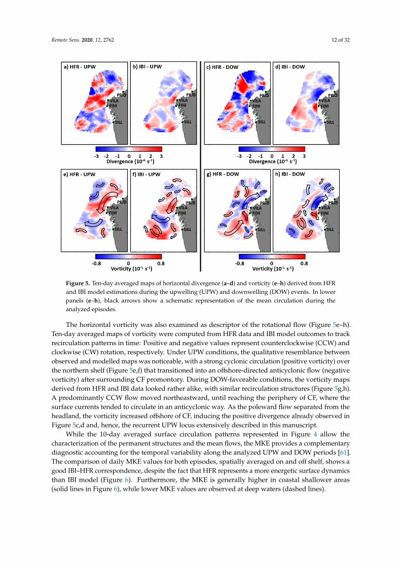
(negative vorticity) after surrounding CF promontory. During DOW-favorable conditions, the vorticity maps derived from HFR and IBI data looked rather alike, with similar recirculation structures (Figure 5g,h). A predominantly CCW flow moved northeastward, until reaching the periphery of CF, where the surface currents tended to circulate in an anticyclonic way. As the poleward flow separated from the headland, the vorticity increased offshore of CF, inducing the positive divergence already observed in Figure 5c,d and, hence, the recurrent UPW locus extensively described in this manuscript.

Figure 5. Ten-day averaged maps of horizontal divergence (a–d) and vorticity (e–h) derived from HFR and IBI model estimations during the upwelling (UPW) and downwelling (DOW) events. In lower panels (e–h), black arrows show a schematic representation of the mean circulation during the analyzed episodes.

While the 10-day averaged surface circulation patterns represented in Figure 4 allow the characterization of the permanent structures and the mean flows, the MKE provides a complementary diagnostic accounting for the temporal variability along the analyzed UPW and DOW periods [61]. The comparison of daily MKE values for both episodes, spatially averaged on and off shelf, shows a good IBI–HFR correspondence, despite the fact that HFR represents a more energetic surface dynamics than IBI model (Figure 6). Furthermore, the MKE is generally higher in coastal shallower areas (solid lines in Figure 6), while lower MKE values are observed at deep waters (dashed lines).

During the UPW event, the upper ocean over the shelf takes only three days for its MKE to reach a prominent peak around 400 (150) cm2·s−2 in the case of HFR (IBI), followed by a steady weakening of the current field (Figure 6a). The evolution of daily MKE in open waters is similar, albeit rather attenuated. This is especially true in the case of IBI, with MKE (red dashed line) smoothly fluctuating in the range (80–100) cm2·s−2. Under DOW conditions, there is a significant correspondence over the shelf between HFR observations and IBI model, with the latter resolving properly both the abrupt rise of MKE during the second half of the event and the peak reached by the seventh day (Figure 6b).

Figure 5. Ten-day averaged maps of horizontal divergence (a–d) and vorticity (e–h) derived from HFRand IBI model estimations during the upwelling (UPW) and downwelling (DOW) events. In lowerpanels (e–h), black arrows show a schematic representation of the mean circulation during theanalyzed episodes.

The horizontal vorticity was also examined as descriptor of the rotational flow (Figure 5e–h).Ten-day averaged maps of vorticity were computed from HFR data and IBI model outcomes to trackrecirculation patterns in time: Positive and negative values represent counterclockwise (CCW) andclockwise (CW) rotation, respectively. Under UPW conditions, the qualitative resemblance betweenobserved and modelled maps was noticeable, with a strong cyclonic circulation (positive vorticity) overthe northern shelf (Figure 5e,f) that transitioned into an offshore-directed anticyclonic flow (negativevorticity) after surrounding CF promontory. During DOW-favorable conditions, the vorticity mapsderived from HFR and IBI data looked rather alike, with similar recirculation structures (Figure 5g,h).A predominantly CCW flow moved northeastward, until reaching the periphery of CF, where thesurface currents tended to circulate in an anticyclonic way. As the poleward flow separated from theheadland, the vorticity increased offshore of CF, inducing the positive divergence already observed inFigure 5c,d and, hence, the recurrent UPW locus extensively described in this manuscript.

While the 10-day averaged surface circulation patterns represented in Figure 4 allow thecharacterization of the permanent structures and the mean flows, the MKE provides a complementarydiagnostic accounting for the temporal variability along the analyzed UPW and DOW periods [61].The comparison of daily MKE values for both episodes, spatially averaged on and off shelf, shows agood IBI–HFR correspondence, despite the fact that HFR represents a more energetic surface dynamicsthan IBI model (Figure 6). Furthermore, the MKE is generally higher in coastal shallower areas(solid lines in Figure 6), while lower MKE values are observed at deep waters (dashed lines).

Remote Sens. 2020, 12, 2762 13 of 32

Remote Sens. 2020, 12, x FOR PEER REVIEW 13 of 32

Such a noticeable increase, higher in the case of HFR, is presumably due to the reported migration of the IPC core from the shelf-break depths to the surface, becoming an intensified northward jet as response to the interplay between stronger DOW-favorable southerly wind regime and the local Galician topography [57]. Again, lower MKE values were observed off shelf during DOW-favorable wind regime (dashed lines).

Changes in daily averaged wind speed (i.e., module), derived from hourly estimations registered at B1 buoy, are in close qualitative agreement with the temporal evolution of MKE values under UPW and DOW states, with no apparent delay in the wind-driven response (Figure 6c,d). Therefore, it seems convenient to further analyze the role of the atmospheric forcing in the modulation of surface circulation.

Figure 6. (a) Evolution of daily mean kinetic energy (MKE) under upwelling (UPW) conditions, averaged over the shelf (solid lines) and open waters (dashed lines), derived from hourly surface currents provided by the HFR (blue color) and IBI model (red). (b) Idem, under downwelling (DOW) conditions. (c,d) Evolution of daily averaged low-pass filtered wind speed (module), derived from hourly estimations at B1 buoy, during the UPW and DOW events, respectively.

3.2.3. Wind Forcing

In order to comprehend, to a greater extent, the correspondence between hourly subtidal circulation and prevalent wind conditions, we calculated CC maps for both UPW and DOW events (Figure 7). At first glance, observed and modelled surface currents seem to be readily induced by the forcing of strong winds, with a spatially averaged CC coefficient of 0.64 and 0.74, respectively, under

Figure 6. (a) Evolution of daily mean kinetic energy (MKE) under upwelling (UPW) conditions,averaged over the shelf (solid lines) and open waters (dashed lines), derived from hourly surfacecurrents provided by the HFR (blue color) and IBI model (red). (b) Idem, under downwelling (DOW)conditions. (c,d) Evolution of daily averaged low-pass filtered wind speed (module), derived fromhourly estimations at B1 buoy, during the UPW and DOW events, respectively.

During the UPW event, the upper ocean over the shelf takes only three days for its MKE to reacha prominent peak around 400 (150) cm2

·s−2 in the case of HFR (IBI), followed by a steady weakeningof the current field (Figure 6a). The evolution of daily MKE in open waters is similar, albeit ratherattenuated. This is especially true in the case of IBI, with MKE (red dashed line) smoothly fluctuatingin the range (80–100) cm2

·s−2. Under DOW conditions, there is a significant correspondence over theshelf between HFR observations and IBI model, with the latter resolving properly both the abruptrise of MKE during the second half of the event and the peak reached by the seventh day (Figure 6b).Such a noticeable increase, higher in the case of HFR, is presumably due to the reported migrationof the IPC core from the shelf-break depths to the surface, becoming an intensified northward jetas response to the interplay between stronger DOW-favorable southerly wind regime and the localGalician topography [57]. Again, lower MKE values were observed off shelf during DOW-favorablewind regime (dashed lines).

Changes in daily averaged wind speed (i.e., module), derived from hourly estimations registeredat B1 buoy, are in close qualitative agreement with the temporal evolution of MKE values underUPW and DOW states, with no apparent delay in the wind-driven response (Figure 6c,d). Therefore,it seems convenient to further analyze the role of the atmospheric forcing in the modulation ofsurface circulation.

Remote Sens. 2020, 12, 2762 14 of 32

3.2.3. Wind Forcing

In order to comprehend, to a greater extent, the correspondence between hourly subtidal circulationand prevalent wind conditions, we calculated CC maps for both UPW and DOW events (Figure 7).At first glance, observed and modelled surface currents seem to be readily induced by the forcingof strong winds, with a spatially averaged CC coefficient of 0.64 and 0.74, respectively, under UPWconditions (Figure 7a,b). By contrast, lower correlation coefficients were identified in the southernmostsector of the spatial coverage.

Remote Sens. 2020, 12, x FOR PEER REVIEW 14 of 32

UPW conditions (Figure 7a,b). By contrast, lower correlation coefficients were identified in the southernmost sector of the spatial coverage.

During the DOW event, higher correlations (above 0.8) were detected in open waters (Figure 7c,d), with a relevant drop (below 0.4) along the Western Iberian continental shelf (Figure 7d). Albeit not as noticeable, a similar tendency was encountered in HFR observations (Figure 7c). Both the HFR and IBI agree to determine a locus of minimum CC in the periphery of CF, indicating that the surface circulation around this coastal promontory might not be primarily driven by wind forcing but likely by a blend of factors, including topo-bathymetric constraints, local wind and tidal effects. The spatially averaged CC coefficients were 0.57 and 0.61 for the observed and modelled flow, respectively.

Figure 7. Maps of complex correlation (CC) index between low-pass filtered hourly wind at B1 buoy and subtidal surface currents provided by the HFR (a,c) and IBI model (b,d), under upwelling (UPW, a,b) and downwelling (DOW, c,d) conditions. Black dot represents B1 buoy.

Complementarily, the time-lagged CC investigation between subtidal currents and low-pass filtered wind time series (not shown) revealed the timely response of the upper layer flow, observed and modelled, to prevalent wind forcing. As expected, a peak of correlation (above 0.8) was generally detected during the first four hours and later accompanied by a gradual decrease in CC coefficient,

Figure 7. Maps of complex correlation (CC) index between low-pass filtered hourly wind at B1 buoyand subtidal surface currents provided by the HFR (a,c) and IBI model (b,d), under upwelling (UPW,a,b) and downwelling (DOW, c,d) conditions. Black dot represents B1 buoy.

During the DOW event, higher correlations (above 0.8) were detected in open waters (Figure 7c,d),with a relevant drop (below 0.4) along the Western Iberian continental shelf (Figure 7d). Albeit notas noticeable, a similar tendency was encountered in HFR observations (Figure 7c). Both the HFRand IBI agree to determine a locus of minimum CC in the periphery of CF, indicating that the surfacecirculation around this coastal promontory might not be primarily driven by wind forcing but likelyby a blend of factors, including topo-bathymetric constraints, local wind and tidal effects. The spatiallyaveraged CC coefficients were 0.57 and 0.61 for the observed and modelled flow, respectively.

Complementarily, the time-lagged CC investigation between subtidal currents and low-passfiltered wind time series (not shown) revealed the timely response of the upper layer flow, observed

Remote Sens. 2020, 12, 2762 15 of 32

and modelled, to prevalent wind forcing. As expected, a peak of correlation (above 0.8) was generallydetected during the first four hours and later accompanied by a gradual decrease in CC coefficient,in accordance with previous works [53,62,63] which reported correlation peaks in the range (0.42–0.64)at zero lag.

3.2.4. Sea Surface Temperature Analysis

The 10-day averaged map of satellite-derived SST and CHL during the UPW episode highlightsthe importance of the coastline orientation (Figure 8a). A marked cooling (below 17 ◦C) along theWestern Galician Coast is evidenced, with surrounding warmer waters reaching up to 19 ◦C. Two maincores of lower SST can be observed: one located to the south of the Rias Baixas and the second one inthe vicinity of CF. Isolines of constant CHL exhibit a spatial distribution in concordance with thermalfronts location. Peaks of CHL (above 7 mg·m−3) are detected close to the western shoreline, thussuggesting accrued injection of subsurface nutrients. By contrast, the sea surface in the NorthernGalician shelf is warmer (around 17.5 ◦C) and not so nutrient-rich, with lower CHL concentrations,lying between 0.2 and 0.5 mg·m−3. These results underline the importance of the coastal orientationand confirm that stronger UPW conditions are developed in the western coast of the NW Iberiansystem, in concordance with References [9,10].

Remote Sens. 2020, 12, x FOR PEER REVIEW 16 of 32

Figure 8. (a) Ten-day averaged map of OSTIA-derived sea surface temperature (SST, colors) and chlorophyll concentration (CHL, isolines) for the upwelling (UPW) event comprised between the 7th and 16th July 2014. (b,c) SST differences between the end and the beginning of the UPW event, computed from OSTIA satellite and IBI model daily estimations, respectively. (d,e) Daily evolution of SST at B1 and B2 buoys location, respectively, as derived from in situ observations (blue line), OSTIA estimations (green line) and IBI model outputs (red line). (f) Ten-day averaged map of OSTIA-derived SST and CHL for the downwelling (DOW) event comprised between the 12th and 21st September 2014. (g,h) SST differences between the end and the beginning of the DOW event, computed from OSTIA satellite and IBI model daily estimations, respectively. (i,j) Daily evolution of SST at B1 and B2 buoys location, respectively, as derived from in situ observations (blue line), OSTIA estimations (green line) and IBI model outputs (red line).

Under DOW conditions, the core of lowest SST (below 18 °C) was confined close to the Northern Galician Coast, wrapped in a strip of warmer waters (around 19.5 °C) that expanded southwestward over the shelf, far beyond B1 location (Figure 8f). The concentration of CHL revealed a significantly lower nutrient fertilization of surface waters, with isolines closer to the western shoreline but, by contrast, more distantly spaced from the northern coast, where a peak of chlorophyll (1 mg·m−3) was detected. By comparing the 10-day averaged maps obtained for UPW (Figure 8a) and DOW (Figure 8f), it can be readily deduced that thermal fronts (i.e., zones with a pronounced horizontal SST gradient) are often associated with higher biological productivity in coastal regions. Such a relationship between front structures and CHL concentration has been previously documented [64,65].

The SST evolution during the DOW episode was also investigated with OSTIA satellite estimations (Figure 8g) and IBI model outputs (Figure 8h). Again, the resemblance between both maps is relevant, with an overall SST increment in coastal areas, ranging from 0.5 to 2 °C. In the case of OSTIA, the warming is smoothly extended over the entire continental shelf and expose a vast peak of 2 °C in the northernmost region, surrounding B2 buoy location (Figure 8g). By contrast, IBI exhibits a narrow belt of warmer waters, confined in shallower coastal areas. A significant increase of SST (above 2 °C) is detected over the edge of the continental break, just in the periphery of B2 buoy

Figure 8. (a) Ten-day averaged map of OSTIA-derived sea surface temperature (SST, colors) andchlorophyll concentration (CHL, isolines) for the upwelling (UPW) event comprised between the 7th and16th July 2014. (b,c) SST differences between the end and the beginning of the UPW event, computedfrom OSTIA satellite and IBI model daily estimations, respectively. (d,e) Daily evolution of SST at B1and B2 buoys location, respectively, as derived from in situ observations (blue line), OSTIA estimations(green line) and IBI model outputs (red line). (f) Ten-day averaged map of OSTIA-derived SST and CHLfor the downwelling (DOW) event comprised between the 12th and 21st September 2014. (g,h) SSTdifferences between the end and the beginning of the DOW event, computed from OSTIA satelliteand IBI model daily estimations, respectively. (i,j) Daily evolution of SST at B1 and B2 buoys location,respectively, as derived from in situ observations (blue line), OSTIA estimations (green line) and IBImodel outputs (red line).

Remote Sens. 2020, 12, 2762 16 of 32

In order to analyze the SST evolution during the 10-day UPW event, the SST difference betweenthe end and the beginning of such episode was explored by means of OSTIA satellite estimations(Figure 8b) and IBI model outputs (Figure 8c). Both share similarities like the overall summer warmingin open-waters or the signal of upwelled waters (cooler than the original surface water), represented bya characteristic band of low SST close to the western coast. However, discrepancies arise in the intensityof the wind-driven cooling, which is broader and more intense in the case of IBI (|∆T| > 2 ◦C), extendedalong the northern shelf in the form of a narrow strip of cool water. On the contrary, remote-sensedestimations indicate a general and relevant warming north of VILA radar site (Figure 8b). An additionaldifference in the modelled SST is the offshore cooling (Figure 8c), probably related to southern cyclonicrecirculation cell (Figure 4b), that is absent from OSTIA map (Figure 8b).

As OSTIA is a satellite-derived product with intrinsic uncertainties, we also used in situ SSTobservations from B1 and B2 buoys as a reference benchmark to elucidate unequivocally the magnitudeof SST variations during the two wind-induced events here analyzed. Since OSTIA is a daily satelliteproduct, hourly estimations from IBI and both buoys were daily averaged, to gain consistency in thedata sampling.

As shown in Figure 8d, in situ observations at B1 (represented by a blue line) exhibit a steeptemperature decrease of 2 ◦C, followed by a slight recovery by the end of the UPW event, with a relatednet cooling of 1.5 ◦C. The modelled SST at the closer grid point (red line), albeit exposing a positive dailybias, is in clear qualitative accordance with in situ observations in terms of temporal evolution and netdecrease of SST under UPW conditions. However, OSTIA estimations at the B1 location (green line)show a moderate drop of 1 ◦C and a marked recovery until reaching back the pre-UPW conditions(18 ◦C), in accordance with the whitish color around B1 in Figure 8b. In situ observations provided byB2 reveal a slight cooling of 0.5 ◦C and a gradual warming during the rest of the episode that led to apositive gradient in temperature (blue line in Figure 8e). Nevertheless, IBI outputs show a sharperdecrease of 1.3 ◦C, followed by a water heating of 1 ◦C and an eventual small SST drop, yielding a finalnegative balance of 0.5 ◦C. This is already shown in Figure 8c, where the high resolution of IBI caneffectively resolve sub-mesoscale dynamics like meanders and the intrusion of UPW filaments off shelf,like the one detached from the coast and presumably wrongly extended northward beyond B2 location.OSTIA estimations (green line) barely captured the SST decrease at the first stage of the UPW event,experiencing later a significant warming until 18.5 ◦C. Despite such a positive bias, satellite-derivedestimations could replicate (and slightly overestimate) the overall warming at B2 location.

Under DOW conditions, the core of lowest SST (below 18 ◦C) was confined close to the NorthernGalician Coast, wrapped in a strip of warmer waters (around 19.5 ◦C) that expanded southwestwardover the shelf, far beyond B1 location (Figure 8f). The concentration of CHL revealed a significantlylower nutrient fertilization of surface waters, with isolines closer to the western shoreline but, bycontrast, more distantly spaced from the northern coast, where a peak of chlorophyll (1 mg·m−3) wasdetected. By comparing the 10-day averaged maps obtained for UPW (Figure 8a) and DOW (Figure 8f),it can be readily deduced that thermal fronts (i.e., zones with a pronounced horizontal SST gradient)are often associated with higher biological productivity in coastal regions. Such a relationship betweenfront structures and CHL concentration has been previously documented [64,65].

The SST evolution during the DOW episode was also investigated with OSTIA satellite estimations(Figure 8g) and IBI model outputs (Figure 8h). Again, the resemblance between both maps is relevant,with an overall SST increment in coastal areas, ranging from 0.5 to 2 ◦C. In the case of OSTIA,the warming is smoothly extended over the entire continental shelf and expose a vast peak of 2 ◦C inthe northernmost region, surrounding B2 buoy location (Figure 8g). By contrast, IBI exhibits a narrowbelt of warmer waters, confined in shallower coastal areas. A significant increase of SST (above 2 ◦C) isdetected over the edge of the continental break, just in the periphery of B2 buoy location and detachedfrom the coast (Figure 8h). Moreover, note that IBI seems to indicate a cooling in the close vicinity ofB1, whereas OSTIA estimations reveal no substantial SST trend in that place (Figure 8g). The daily SSTevolution registered at B1 buoy exhibits a net decrease of temperature, with an abrupt drop of 2 ◦C

Remote Sens. 2020, 12, 2762 17 of 32

during the first days and a moderate recovery afterward (blue line, Figure 8i). The IBI model (red line),despite the observed bias (1 ◦C) in the daily outputs at the grid point closer to B1 emplacement,seems to properly resolve the overall cooling of 1 ◦C during the DOW event. On the contrary, OSTIAestimations scarcely captured the SST drop and the subsequent warming, reflecting a negligible SSTvariation between the first and the last day of the analyzed DOW episode. The situation at B2 locationwas, conversely, rather different (Figure 8j). The SST collected at B2 (blue line) experienced an abruptincrease, followed by an equivalent sharp drop and again by an eventual increase of almost 2 ◦C.The IBI model (red line) failed to capture those oscillations but agreed to reproduce adequately thenet warming, with rather similar initial and final SST values. This time, OSTIA remote estimationsproperly reproduced the ocean water heating, despite the water temperature overestimation by theend of the event.

3.2.5. Vertical Analysis

In this section, the IBI model outputs were compared against independent (i.e., not assimilated)profiles of temperature and salinity, collected during the entire summer 2014, at one CTD stationdeployed inside of Rias Baixas (V5, denoted in Figure 1b), with the aim of portraying the verticalstructure and gaining an improved insight into the three-dimensional flow geometry under UPW andDOW conditions. To this aim, IBI daily estimations at the closest grid point were used.

As shown in Figure 9a,b, the IBI–CTD accordance in the temporal evolution of the temperaturefield is relevant. The IBI performance appears to be sound in terms of timing, intensity and verticalextension of successive water-cooling and -warming episodes, likely related to the alternation ofwind-driven UPW and DOW conditions, respectively. Especially relevant is the increase of temperatureby the second half of September, where the subduction of warmer waters (20 ◦C) reached 30 m indepth. The agreement between CTD observations and IBI estimations, in terms of onset, strength andduration of this DOW event, is significantly high, as reflected by the moderate differences, evidencedin Figure 9c. By contrast, higher discrepancies can be observed in July 2014 when the main UPW eventanalyzed here took place. Negative differences seem to indicate that IBI overestimated the verticaluplift of colder waters (Figure 9c).

With regards to the salinity field (Figure 10), the model appeared to overrate the noticeableintrusion of fresher (33.5 PSU) waters into deeper levels (up to 25 m depth), related to downwardmotions under dominant southerly wind conditions (Figure 10b). However, IBI properly capturedthe upward flux of deep, dense and saltier (35.5 PSU) waters into the sea surface for several dates(14th and 28th of July, and 19th of August) coincident with UPW-favorable events, as indicated by thenegligible differences observed in Figure 10c.

In order to get a more realistic diagnosis of IBI three-dimensional performance, instead ofcomputing the bias (where positive and negative differences might partially cancel each other, leadingto a more benevolent skill score), the mean absolute difference (MAD), vertically averaged over theentire study period, was used. A MAD of 0.79 ◦C (0.48 PSU) was derived from the IBI–CTD comparisonfor the temperature and salinity fields, respectively. Similar qualitative results were recently reportedby Reference [66] during a validation experiment of a MOHID modelling suite against V5 CTD station.

Remote Sens. 2020, 12, 2762 18 of 32Remote Sens. 2020, 12, x FOR PEER REVIEW 18 of 32

Figure 9. Comparison of temperature (TMP) profiles registered at V5 station (denoted in Figure 1b) by a CDT device (a) and IBI model (b) at the closest grid point. (c) Differences of TMP between the modelled and the observed profiles. Note that this figure is not a Hovmöller diagram but a temporal concatenation of specific dates: Only those CTD in situ observations that successfully fulfilled the quality control have been depicted.

Figure 9. Comparison of temperature (TMP) profiles registered at V5 station (denoted in Figure 1b)by a CDT device (a) and IBI model (b) at the closest grid point. (c) Differences of TMP between themodelled and the observed profiles. Note that this figure is not a Hovmöller diagram but a temporalconcatenation of specific dates: Only those CTD in situ observations that successfully fulfilled thequality control have been depicted.

Remote Sens. 2020, 12, 2762 19 of 32Remote Sens. 2020, 12, x FOR PEER REVIEW 19 of 32

Figure 10. Comparison of salinity (SAL) profiles registered at V5 station (denoted in Figure 1b) by a CDT device (a) and IBI model (b) at the closest grid point. (c) Differences of SAL between the modelled and the observed profiles. Note that this figure is not a Hovmöller diagram but a temporal concatenation of specific dates: Only those CTD in situ observations that successfully fulfilled the quality control have been depicted.

3.3. New HFR-Derived Upwelling Index: UIHFR

In order to assess the consistency of the proposed UIHFR, an annual validation against two preexisting coastal UIs was conducted for the entire 2014. According to the best linear fit of scatterplot between UIHFR y UIBAIXAS, the agreement between this novel ocean-based index and UIBAIXAS seemed to be significantly high (Figure 11a). The slope and the correlation coefficient were close to 1 and 0.8, respectively. The comparison against UIB1 (not shown) revealed a moderate agreement, with a lower correlation coefficient (0.49).

Figure 10. Comparison of salinity (SAL) profiles registered at V5 station (denoted in Figure 1b) bya CDT device (a) and IBI model (b) at the closest grid point. (c) Differences of SAL between themodelled and the observed profiles. Note that this figure is not a Hovmöller diagram but a temporalconcatenation of specific dates: Only those CTD in situ observations that successfully fulfilled thequality control have been depicted.

3.3. New HFR-Derived Upwelling Index: UIHFR

In order to assess the consistency of the proposed UIHFR, an annual validation against twopreexisting coastal UIs was conducted for the entire 2014. According to the best linear fit of scatterplotbetween UIHFR y UIBAIXAS, the agreement between this novel ocean-based index and UIBAIXAS seemedto be significantly high (Figure 11a). The slope and the correlation coefficient were close to 1 and 0.8,respectively. The comparison against UIB1 (not shown) revealed a moderate agreement, with a lowercorrelation coefficient (0.49).

Remote Sens. 2020, 12, 2762 20 of 32

Remote Sens. 2020, 12, x FOR PEER REVIEW 20 of 32

The temporal evolution of monthly averaged UIs showed that UIHFR could appropriately reproduce the annual cycle along 2014, with a predominant UPW phase during the central part of the year (May–July) and prevailing DOW-favorable conditions during the rest of the months (Figure 11 b). The visual resemblance with UIBAIXAS is noticeable, although UIHFR appears to generally overestimate the intensity of DOW scenarios. In contrast, the accordance with UIB1 was substantially lower despite the similar evolution.

The spatial distribution of the monthly UIHFR values exhibited recurrent features over the Galician continental shelf (Figure 11c–f). During DOW-favorable months, this coastal index persistently reached two localized minimums in the periphery of SILL and VILA radar sites. In February, UIHFR dropped to −4800 m3·s−1·km−1 (Figure 11c). In September, it only decreased until −3900 m3·s−1·km−1 in the vicinity of SILL site. A secondary minimum, less intense (about −2000 m3·s−1·km−1), was detected in northern areas, around the VILA site (Figure 11f). By contrast, a prominent peak of UIHFR (~3000 m3·s−1·km−1) was confined in the southernmost region under UPW-favorable conditions in May (Figure 11d). Later, a dipole-like structure was observed in July (Figure 11e), with two main cores of maximum UIHFR (close to 2000 m3·s−1·km−1). Since both cores were coincident with each center of cooler and fertilized water previously evidenced in the satellite-derived SST and CHL map (Figure 8a), these results seem to confirm the viability of the proposed HFR-derived index.

Figure 11. (a) Best linear fit of scatter plot between two different coastal upwelling indexes, for the entire year 2014; (b) Annual (2014) evolution of monthly-averaged coastal upwelling indexes: upwelling index based on HFR-derived hourly surface current observations (UIHFR) = red line, upwelling index based on hourly data of sea level pressure (UIBAIXAS) = blue line and upwelling index based on wind (UIB1) = green line. (c–f) Spatial distribution of monthly averaged UIHFR over the Galician continental shelf under predominant DOW (c,f) and UPW (d,e) conditions. Bathymetric contour shows depth at 400 m.

Figure 11. (a) Best linear fit of scatter plot between two different coastal upwelling indexes, for the entireyear 2014; (b) Annual (2014) evolution of monthly-averaged coastal upwelling indexes: upwellingindex based on HFR-derived hourly surface current observations (UIHFR) = red line, upwelling indexbased on hourly data of sea level pressure (UIBAIXAS) = blue line and upwelling index based on wind(UIB1) = green line. (c–f) Spatial distribution of monthly averaged UIHFR over the Galician continentalshelf under predominant DOW (c,f) and UPW (d,e) conditions. Bathymetric contour shows depth at400 m.

The temporal evolution of monthly averaged UIs showed that UIHFR could appropriately reproducethe annual cycle along 2014, with a predominant UPW phase during the central part of the year(May–July) and prevailing DOW-favorable conditions during the rest of the months (Figure 11b).The visual resemblance with UIBAIXAS is noticeable, although UIHFR appears to generally overestimatethe intensity of DOW scenarios. In contrast, the accordance with UIB1 was substantially lower despitethe similar evolution.

The spatial distribution of the monthly UIHFR values exhibited recurrent features over the Galiciancontinental shelf (Figure 11c–f). During DOW-favorable months, this coastal index persistently reachedtwo localized minimums in the periphery of SILL and VILA radar sites. In February, UIHFR dropped to−4800 m3

·s−1·km−1 (Figure 11c). In September, it only decreased until −3900 m3

·s−1·km−1 in the vicinity

of SILL site. A secondary minimum, less intense (about −2000 m3·s−1·km−1), was detected in northern

areas, around the VILA site (Figure 11f). By contrast, a prominent peak of UIHFR (~3000 m3·s−1·km−1)

was confined in the southernmost region under UPW-favorable conditions in May (Figure 11d). Later,a dipole-like structure was observed in July (Figure 11e), with two main cores of maximum UIHFR

(close to 2000 m3·s−1·km−1). Since both cores were coincident with each center of cooler and fertilized

water previously evidenced in the satellite-derived SST and CHL map (Figure 8a), these results seemto confirm the viability of the proposed HFR-derived index.

Remote Sens. 2020, 12, 2762 21 of 32

With the purpose of gaining further insight into the capabilities of the new UIHFR, we selected avariety of UPW and DOW events of diverse duration and strength, during summer 2014, and latercharacterized them by means of IROS metric. During July, the evolution of the three UIs sharedsome similarities (Figure 12a): three UPW episodes were clearly evidenced (persistently positive UImagnitudes), while a short and more elusive DOW event was categorized according to UIBAIXAS andUIB1 negative values. Both the time-averaged surface circulation and the spatial distribution of IROSunder UPW conditions presented common peculiarities (Figure 12b,c,e). A prominent peak of IROSwas clearly evidenced along the northern shallower coastal waters, expanding westward offshore inthe form of a longitudinal belt (Figure 12b,c). As a result of a temporal outage that affected the northernHFR sites, the spatial coverage was substantially reduced during the last part of the month (Figure 12e).However, the strip of higher IROS values was still partially observable. By contrast, the surfacecirculation and IROS patterns related to the short DOW episode were kind of noisy (Figure 12d).

Remote Sens. 2020, 12, x FOR PEER REVIEW 21 of 32

With the purpose of gaining further insight into the capabilities of the new UIHFR, we selected a variety of UPW and DOW events of diverse duration and strength, during summer 2014, and later characterized them by means of IROS metric. During July, the evolution of the three UIs shared some similarities (Figure 12a): three UPW episodes were clearly evidenced (persistently positive UI magnitudes), while a short and more elusive DOW event was categorized according to UIBAIXAS and UIB1 negative values. Both the time-averaged surface circulation and the spatial distribution of IROS under UPW conditions presented common peculiarities (Figure 12b,c,e). A prominent peak of IROS was clearly evidenced along the northern shallower coastal waters, expanding westward offshore in the form of a longitudinal belt (Figure 12b,c). As a result of a temporal outage that affected the northern HFR sites, the spatial coverage was substantially reduced during the last part of the month (Figure 12e). However, the strip of higher IROS values was still partially observable. By contrast, the surface circulation and IROS patterns related to the short DOW episode were kind of noisy (Figure 12d).

Figure 12. (a) Temporal evolution of hourly UIHFR (red line) and 6-hourly UIBAIXAS (blue squares) and UIB1 (green dots) during July 2014. Gray boxes indicate four selected UPW and DOW episodes; (b–e) Maps of time-averaged circulation and Instantaneous Rate of Separation (IROS) for each specific event. IROS magnitudes are normalized by the absolute value of the Coriolis parameter f.

Figure 12. (a) Temporal evolution of hourly UIHFR (red line) and 6-hourly UIBAIXAS (blue squares)and UIB1 (green dots) during July 2014. Gray boxes indicate four selected UPW and DOW episodes;(b–e) Maps of time-averaged circulation and Instantaneous Rate of Separation (IROS) for each specificevent. IROS magnitudes are normalized by the absolute value of the Coriolis parameter f.

Remote Sens. 2020, 12, 2762 22 of 32

During August 2014, the resemblance between the three different Uis was again noticeable(Figure 13a). A relevant peak of UPW (above 4000 m3

·s−1·km−1) was captured by each UI,

although UIHFR indicated not only more intense UPW conditions but also anticipated in the timeline.Four different episodes were eventually categorized. The first one, comprised between the 11th and14th of August, was chosen according to high UIHFR values, while the other remaining indexes indicatedweak UPW or even DOW conditions. However, the time-averaged map of surface currents confirmedthe typical offshore deflection of the flow, associated with UPW-favorable conditions (Figure 13b).Equally, we could get a glimpse of the aforementioned belt of high IROS magnitudes between FINIand VILA sites, despite the limited areal coverage. Two additional UPW events were selected, andthe resulting time-averaged maps revealed similar characteristics in terms of surface circulation andIROS distribution (Figure 13c,e), in spite of the different time span (nine days versus two days).Again, a rather noisy circulation map was obtained under DOW conditions (Figure 13d), although alongitudinal belt of high IROS values was still present between FINI and VILA sites. These peculiaritieswere in clear accordance with the previous DOW event analyzed in July (Figure 12d).

Remote Sens. 2020, 12, x FOR PEER REVIEW 22 of 32

During August 2014, the resemblance between the three different Uis was again noticeable (Figure 13a). A relevant peak of UPW (above 4000 m3·s−1·km−1) was captured by each UI, although UIHFR indicated not only more intense UPW conditions but also anticipated in the timeline. Four different episodes were eventually categorized. The first one, comprised between the 11th and 14th of August, was chosen according to high UIHFR values, while the other remaining indexes indicated weak UPW or even DOW conditions. However, the time-averaged map of surface currents confirmed the typical offshore deflection of the flow, associated with UPW-favorable conditions (Figure 13b). Equally, we could get a glimpse of the aforementioned belt of high IROS magnitudes between FINI and VILA sites, despite the limited areal coverage. Two additional UPW events were selected, and the resulting time-averaged maps revealed similar characteristics in terms of surface circulation and IROS distribution (Figure 13c,e), in spite of the different time span (nine days versus two days). Again, a rather noisy circulation map was obtained under DOW conditions (Figure 13d), although a longitudinal belt of high IROS values was still present between FINI and VILA sites. These peculiarities were in clear accordance with the previous DOW event analyzed in July (Figure 12d).

Figure 13. (a) Temporal evolution of hourly UIHFR (red line) and six-hourly UIBAIXAS (blue squares) and UIB1 (green dots) during August 2014. Gray boxes indicate four selected UPW and DOW episodes. (b–e) Maps of time-averaged circulation and Instantaneous Rate of Separation (IROS) for each specific event. IROS magnitudes are normalized by the absolute value of the Coriolis parameter, f.

Figure 13. (a) Temporal evolution of hourly UIHFR (red line) and six-hourly UIBAIXAS (blue squares)and UIB1 (green dots) during August 2014. Gray boxes indicate four selected UPW and DOW episodes.(b–e) Maps of time-averaged circulation and Instantaneous Rate of Separation (IROS) for each specificevent. IROS magnitudes are normalized by the absolute value of the Coriolis parameter, f.

During September 2014, the three indexes generally looked alike (Figure 14a) and jointly identifieda relatively weak two-day DOW episode (days five and six). The associated circulation pattern depictedthe well-documented poleward flow (Figure 14b). A delimited peak of IROS was observed, confined

Remote Sens. 2020, 12, 2762 23 of 32

in coastal areas between FIST and VILA sites. A strong DOW event was classified according to theextremely persistent negative values of UIHFR and UIBAIXAS (around −6000 m3

·s−1·km−1). Again,

the surface waters flowed northward with higher IROS values detected over the shelf break and theNW sector (Figure 14c). Between the 22nd and 25th of September, UIBAIXAS and UIB1 indicated theexistence of predominant UPW conditions, in opposition to UIHFR, which simply denoted a steadyrelaxation of DOW until reaching a calm state (Figure 14a). The related circulation pattern indeedexhibited a prevailing poleward flow over the shelf, whereas a cyclonic recirculation could be observedin the southernmost sector of the HFR domain, likely induced by northerly winds that started toconstantly blow (Figure 14d). Finally, a brief DOW event (27–28 of September) was selected accordingto UIHFR negative values, although the other two indexes reflected calm conditions. The associatedmap of surface currents confirmed the validity of the proposed ocean-based index: The flow waseffectively oriented to the north, and an elongated strip of high IROS values was encountered alongthe shelf break (Figure 14e).

Remote Sens. 2020, 12, x FOR PEER REVIEW 23 of 32

During September 2014, the three indexes generally looked alike (Figure 14a) and jointly identified a relatively weak two-day DOW episode (days five and six). The associated circulation pattern depicted the well-documented poleward flow (Figure 14b). A delimited peak of IROS was observed, confined in coastal areas between FIST and VILA sites. A strong DOW event was classified according to the extremely persistent negative values of UIHFR and UIBAIXAS (around −6000 m3·s−1·km−1). Again, the surface waters flowed northward with higher IROS values detected over the shelf break and the NW sector (Figure 14c). Between the 22nd and 25th of September, UIBAIXAS and UIB1 indicated the existence of predominant UPW conditions, in opposition to UIHFR, which simply denoted a steady relaxation of DOW until reaching a calm state (Figure 14a). The related circulation pattern indeed exhibited a prevailing poleward flow over the shelf, whereas a cyclonic recirculation could be observed in the southernmost sector of the HFR domain, likely induced by northerly winds that started to constantly blow (Figure 14d). Finally, a brief DOW event (27–28 of September) was selected according to UIHFR negative values, although the other two indexes reflected calm conditions. The associated map of surface currents confirmed the validity of the proposed ocean-based index: The flow was effectively oriented to the north, and an elongated strip of high IROS values was encountered along the shelf break (Figure 14e).

Figure 14. (a) Temporal evolution of hourly UIHFR (red line) and 6-hourly UIBAIXAS (blue squares) and UIB1 (green dots) during September 2014. Gray boxes indicate four selected UPW and DOW episodes. (b–e) Maps of time-averaged circulation and Instantaneous Rate of Separation (IROS) for each specific event. Bathymetric contour shows depth at 400 m. IROS magnitudes are normalized by the absolute value of the Coriolis parameter, f.

Figure 14. (a) Temporal evolution of hourly UIHFR (red line) and 6-hourly UIBAIXAS (blue squares) andUIB1 (green dots) during September 2014. Gray boxes indicate four selected UPW and DOW episodes.(b–e) Maps of time-averaged circulation and Instantaneous Rate of Separation (IROS) for each specificevent. Bathymetric contour shows depth at 400 m. IROS magnitudes are normalized by the absolutevalue of the Coriolis parameter, f.

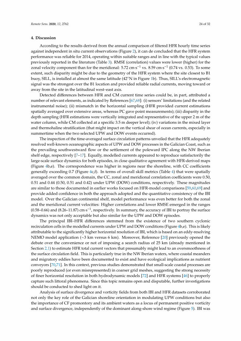
Remote Sens. 2020, 12, 2762 24 of 32

4. Discussion

According to the results derived from the annual comparison of filtered HFR hourly time seriesagainst independent in situ current observations (Figure 2), it can de concluded that the HFR systemperformance was reliable for 2014, operating within suitable ranges and in line with the typical valuespreviously reported in the literature (Table 3). RMSE (correlation) values were lower (higher) for thezonal velocity component than for the meridional: 5.72 cm·s−1 vs. 8.59 cm·s−1 (0.74 vs. 0.53). To someextent, such disparity might be due to the geometry of the HFR system where the site closest to B1buoy, SILL, is installed at almost the same latitude (42◦N in Figure 1b). Thus, SILL’s electromagneticsignal was the strongest over the B1 location and provided reliable radial currents, moving toward oraway from the site in the latitudinal west–east axis.

Detected differences between HFR and CM current time series could be, in part, attributed anumber of relevant elements, as indicated by References [67,68]: (i) sensors’ limitations (and the relatedinstrumental noise); (ii) mismatch in the horizontal sampling (HFR provided current estimationsspatially averaged over extensive areas, whereas PC gave point measurements); (iii) disparity in thedepth sampling (HFR estimations were vertically integrated and representative of the upper 2 m of thewater column, while CM collected at a specific 3.5 m deeper level); (iv) variations in the mixed layerand thermohaline stratification (that might impact on the vertical shear of ocean currents, especially insummertime when the two selected UPW and DOW events occurred).

The inspection of the time-averaged surface circulation patterns unveiled that the HFR adequatelyresolved well-known oceanographic aspects of UPW and DOW processes in the Galician Coast, such asthe prevailing southwestward flow or the settlement of the poleward IPC along the NW Iberianshelf edge, respectively [7–17]. Equally, modelled currents appeared to reproduce satisfactorily thelarge-scale surface dynamics for both episodes, in close qualitative agreement with HFR-derived maps(Figure 4b,e). The correspondence was higher in regions near the shoreline, with CC coefficientsgenerally exceeding 0.7 (Figure 4c,f). In terms of overall skill metrics (Table 4) that were spatiallyaveraged over the common domain, the CC, zonal and meridional correlation coefficients were 0.50,0.51 and 0.44 (0.50, 0.51 and 0.42) under UPW (DOW) conditions, respectively. These magnitudesare similar to those documented in earlier works focused on HFR-model comparisons [59,60,69] andprovide added confidence in both the approach adopted and the quantitative consistency of the IBImodel. Over the Galician continental shelf, model performance was even better for both the zonaland the meridional current velocities: Higher correlations and lower RMSE emerged in the ranges(0.58–0.66) and (8.26–11.87) cm·s−1, respectively. In summary, the accuracy of IBI to portray the surfacedynamics was not only acceptable but also similar for the UPW and DOW episodes.

The principal IBI–HFR differences stemmed from the existence of two southern cyclonicrecirculation cells in the modelled currents under UPW and DOW conditions (Figure 4b,e). This is likelyattributable to the significantly higher horizontal resolution of IBI, which is based on an eddy-resolvingNEMO model application (∼3 km versus 6 km). Moreover, Reference [20] previously opened thedebate over the convenience or not of imposing a search radius of 25 km (already mentioned inSection 2.1) to estimate HFR total current vectors that presumably might lead to an oversmoothness ofthe surface circulation field. This is particularly true in the NW Iberian waters, where coastal meandersand migratory eddies have been documented to exist and have ecological implications as nutrientconveyors [70,71]. In this context, previous studies demonstrated that small-scale coastal processes arepoorly reproduced (or even misrepresented) in coarser grid meshes, suggesting the strong necessityof finer horizontal resolution in both hydrodynamic models [72] and HFR systems [46] to properlycapture such littoral phenomena. Since this topic remains open and disputable, further investigationsshould be conducted to shed light on it.

Analysis of surface divergence and vorticity fields from both IBI and HFR datasets corroboratednot only the key role of the Galician shoreline orientation in modulating UPW conditions but alsothe importance of CF promontory and its ambient waters as a locus of permanent positive vorticityand surface divergence, independently of the dominant along-shore wind regime (Figure 5). IBI was

Remote Sens. 2020, 12, 2762 25 of 32

apparently successful at reproducing broad-scale features of the HFR-derived patterns of divergenceand vorticity. To the authors’ knowledge, this is the first attempt to characterize UPW and DOWconditions in the Galician waters by means of divergence and vorticity fields derived from bothhourly modelled and remote-sensed surface currents. Similar initiatives were effectively addressedin the west coast of the USA [26,27,29], also identifying localized areas of positive divergence at thetip of headlands, such as Point Loma [26] or Point Reyes [27] in California, that ultimately inducedtopographic upwelling. With regards to the main discrepancies between the modelled and observedvorticity, they were identified in the southern sector of the common spatial domain (Figure 5f,h).Two broad cores of positive vorticity were found in IBI outcomes, presumably associated with thecoherent and elongated vortexes in the along-shore direction previously described (Figure 4b,e).Over the rest of the domain, the IBI–HFR correspondence was fairly good.

Spatially averaged MKE was computed as an ancillary indicator of the temporal variability of theflow during the selected UPW and DOW periods (Figure 6). Although IBI statistically reproducedthe daily evolution of MKE, the overall kinetic energy of the modelled currents was lower, indicatingthat a fraction of the total flow variance was not entirely replicated. Similar conclusions in relationto the limited kinematic content of the modelled flow were previously drawn by References [59,60].The moderate but systematic underestimation of IBI currents energy at the uppermost level mightbe related to a limited representation of vertical stratification during the warm summer period.Indeed, results exposed in Section 3.2.5 of this paper seem to confirm this conjecture, as IBI tendedto overestimate (in intensity and spatial extension) both the cooling and warming during the UPWand DOW episodes, respectively (Figure 9), thus driving an enhanced vertical mixing that might havepartially slowed down the wind-induced currents speed.

The relationship of atmospheric forcing and flow variability was analyzed by means of CCmaps between the wind collected at B1 buoy and observed and modelled surface currents (Figure 7).Results appeared to indicate a relevant sensitivity of IBI ocean forecast system to wind stressesin the Galician tidally dominated environment. A time-lagged vector correlation analysis wasapplied to investigate the reaction of the upper-layer circulation for a 24-hour interval (not shown).Maximum correlations (above 0.7) were found during the first four hours, illustrating that only a brieftime is required for the subtidal current to establish the equilibrium with local wind, thus staying inconformity with Reference [56,73]. Once again, HFR and IBI exhibited a similar qualitative performance.Notwithstanding, results should be interpreted with caution since the spatial inhomogeneity of thewind field in Galicia has been previously suggested [10,56]. Although Reference [74] acknowledgedthat B1 buoy was free of possible errors in the correction of the terrain roughness and was, hence,the better station to represent ocean–atmosphere interactions at both Rias Baixas and the adjacentwestern shelf, local wind in the complex Northern Galician Coast may substantially differ and cause adecrease of maximum correlation between wind and surface currents.

The 10-day averaged map of satellite-derived SST and CHL during the UPW and DOWevents confirmed the relevance of the Galician coastline’s shape (Figure 8). Abrupt changesin coastal orientation can induce noticeable wind stress fluctuations and, hence, different UPWconditions with subsequent biophysical implications, as here observed and previously documented byReferences [9,10,12,56]. Stronger upwelling, with cooler and more enriched waters, was evidenced inthe Western Galician shelf [9,10].

The comparison of the SST field observed by OSTIA mission and modelled by IBI during the UPWevent revealed interesting differences. Despite sharing similar features, the intensity of the wind-drivencooling was broader and more intense in the case of IBI. These results are in line with a recent workpublished by Reference [75] where a variety of L4 satellite-derived SST products (including OSTIA)were reported to underestimate the thermal fingerprint of strong coastal UPW, not only in the NWIberian system but also in other regions worldwide. While performing satisfactorily over broadareas for most of the year, such products seemed to misrepresent UPW-induced abrupt temperaturetransitions in coastal waters. Notwithstanding, it is worth noting that both in situ and remote-sensing

Remote Sens. 2020, 12, 2762 26 of 32

devices are affected by technical limitations and intrinsic uncertainties so SST observations from B1and B2 buoys should only be considered as a close approximation of “ground truth”.

Additionally, IBI model daily outputs were compared against temperature and salinity profilescollected at one CTD station, with the aim of gaining further insight into the three-dimensional flowgeometry under UPW and DOW conditions (Figures 9 and 10). Therefore, the skill metrics herepresented appear to indicate that IBI represented appropriately the main signatures of the verticalthermohaline structure along summer 2014 in the intricate Rias Baixas, where the irregular coastalmorphology and abrupt gradients in local bathymetry might handicap precise hydrodynamic modelsforecast. Focusing on the UPW event here studied (7th–16th July), we see that the results seem tosuggest that IBI misrepresented, to some extent, the associated cooling, but accurately resolved theassociated salinity variability. On the contrary, the model slightly overestimated the temperature ofsinking water masses under persistent DOW conditions (12th–21st September), but failed to capturetheir salinity. Nonetheless, since this is a single isolated example, ancillary validation exercises alongthe Galician Coast should be performed in the future. The detected discrepancies within the Rias Baixasmight be in part attributed to discordant time sampling: While CTD devices capture instantaneouspictures of the water column state, the IBI model provides daily averaged estimations that couldhypothetically include high-frequency effects of a variety of coastal processes, including riverinefreshwater discharges, tidal mixing or land–sea breezes.

A variety of constraint factors inherently restrict the IBI–HFR comparison and must be taken intoaccount when interpreting the results previously exposed. Such elements encompass remote-sensorlimitations and the aforementioned GDOP, discrepancies in both the depth sampling and the horizontalgrid mesh, or any potential limitation in the meteorological forcing used to run IBI ocean forecastingsystem (which is out of the scope of the present paper but probably deserves a detailed examinationelsewhere). In the same line, model comparisons against in situ buoys, satellite-derived SST productsor CTD profiles are handicapped by similar idiosyncratic aspects. As data assimilation providesthe integrative framework for maximizing the joint utility of observations and ocean forecastingsystems, a SAM-2 assimilation scheme [76] was later incorporated in the following version of IBIsystem (released in April 2018). Since then, altimetry data (along-track sea-level anomalies), OSTIA SSTproduct and CORA (Coriolis Ocean database ReAnalysis) datasets (including ARGO, gliders, driftingbuoys, etc.) are routinely assimilated into IBI operational chain in order to enhance its predictiveskills. Additional efforts should be also devoted to optimizing the observations-model strategy bycombining HFR synoptic circulation maps and high-resolution coastal simulations. In this context,classic observing system experiments (OSEs) could be useful to evaluate the impact of assimilatingHFR data on model prognostic capabilities.

With the aim of characterizing the variability of the NW Iberian UPW system, a novel and rathersimple coastal UPW index was generated from HFR-derived hourly surface current estimations, theso-called UIHFR. Assuming the prompt and direct reaction of the upper ocean layer to intense andprolonged wind forcing, we think it seemed reasonable to develop an ocean-based proxy of UPW andDOW conditions. The proposed high-frequency index was compared with two preexisting six-hourlyUPW indexes for the entire 2014. Results confirmed the consistency of UIHFR in terms of mean valuesand temporal variability (Figure 11a,b). The spatial distribution of UIHFR along the Galician continentalshelf was also sound (Figure 11c–f). The map of UIHFR corresponding to July (Figure 11e) matchedwell with the remotely sensed SST and CHL fields associated with the 10-day UPW event (Figure 8a),confirming the existence of relevant biophysical interactions in the NW Iberian coastal UPW system.

The skill of UIHFR to categorize and describe UPW and DOW events during summer 2014 was alsoqualitatively evaluated. The most intense episodes were properly captured by UIHFR, in agreementwith the other two indexes (Figures 12a, 13a and 14a). Discrepancies arise from relatively short eventsof moderate intensity: While UIBAIXAS and UIB1 indicated predominant DOW (Figures 12a and 13a)and UPW (Figure 14a) conditions, UIHFR appeared to contradict the formers, revealing by contrastrelaxation episodes (i.e., UIHFR values close to zero). The related time-averaged circulation maps

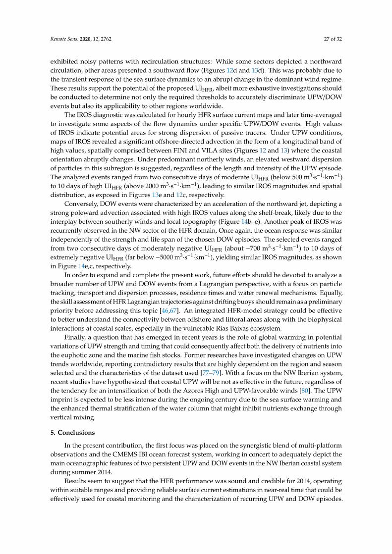
Remote Sens. 2020, 12, 2762 27 of 32

exhibited noisy patterns with recirculation structures: While some sectors depicted a northwardcirculation, other areas presented a southward flow (Figures 12d and 13d). This was probably due tothe transient response of the sea surface dynamics to an abrupt change in the dominant wind regime.These results support the potential of the proposed UIHFR, albeit more exhaustive investigations shouldbe conducted to determine not only the required thresholds to accurately discriminate UPW/DOWevents but also its applicability to other regions worldwide.

The IROS diagnostic was calculated for hourly HFR surface current maps and later time-averagedto investigate some aspects of the flow dynamics under specific UPW/DOW events. High valuesof IROS indicate potential areas for strong dispersion of passive tracers. Under UPW conditions,maps of IROS revealed a significant offshore-directed advection in the form of a longitudinal band ofhigh values, spatially comprised between FINI and VILA sites (Figures 12 and 13) where the coastalorientation abruptly changes. Under predominant northerly winds, an elevated westward dispersionof particles in this subregion is suggested, regardless of the length and intensity of the UPW episode.The analyzed events ranged from two consecutive days of moderate UIHFR (below 500 m3

·s−1·km−1)

to 10 days of high UIHFR (above 2000 m3·s−1·km−1), leading to similar IROS magnitudes and spatial

distribution, as exposed in Figures 13e and 12c, respectively.Conversely, DOW events were characterized by an acceleration of the northward jet, depicting a

strong poleward advection associated with high IROS values along the shelf-break, likely due to theinterplay between southerly winds and local topography (Figure 14b–e). Another peak of IROS wasrecurrently observed in the NW sector of the HFR domain, Once again, the ocean response was similarindependently of the strength and life span of the chosen DOW episodes. The selected events rangedfrom two consecutive days of moderately negative UIHFR (about −700 m3

·s−1·km−1) to 10 days of

extremely negative UIHFR (far below −5000 m3·s−1·km−1), yielding similar IROS magnitudes, as shown

in Figure 14e,c, respectively.In order to expand and complete the present work, future efforts should be devoted to analyze a

broader number of UPW and DOW events from a Lagrangian perspective, with a focus on particletracking, transport and dispersion processes, residence times and water renewal mechanisms. Equally,the skill assessment of HFR Lagrangian trajectories against drifting buoys should remain as a preliminarypriority before addressing this topic [46,67]. An integrated HFR-model strategy could be effectiveto better understand the connectivity between offshore and littoral areas along with the biophysicalinteractions at coastal scales, especially in the vulnerable Rias Baixas ecosystem.

Finally, a question that has emerged in recent years is the role of global warming in potentialvariations of UPW strength and timing that could consequently affect both the delivery of nutrients intothe euphotic zone and the marine fish stocks. Former researches have investigated changes on UPWtrends worldwide, reporting contradictory results that are highly dependent on the region and seasonselected and the characteristics of the dataset used [77–79]. With a focus on the NW Iberian system,recent studies have hypothesized that coastal UPW will be not as effective in the future, regardless ofthe tendency for an intensification of both the Azores High and UPW-favorable winds [80]. The UPWimprint is expected to be less intense during the ongoing century due to the sea surface warming andthe enhanced thermal stratification of the water column that might inhibit nutrients exchange throughvertical mixing.

5. Conclusions

In the present contribution, the first focus was placed on the synergistic blend of multi-platformobservations and the CMEMS IBI ocean forecast system, working in concert to adequately depict themain oceanographic features of two persistent UPW and DOW events in the NW Iberian coastal systemduring summer 2014.

Results seem to suggest that the HFR performance was sound and credible for 2014, operatingwithin suitable ranges and providing reliable surface current estimations in near-real time that could beeffectively used for coastal monitoring and the characterization of recurring UPW and DOW episodes.

Remote Sens. 2020, 12, 2762 28 of 32

Furthermore, the examination of HFR-derived surface circulation patterns confirms that this land-basedtechnology properly resolved well-known oceanographic aspects of the Galician UPW and DOWprocesses, in accordance with the historical literature.

The significant resemblance between observed and modelled wind-driven currents revealedthe strong connectivity between offshore and coastal ecosystems and also confirmed the importanceof CF promontory as a locus of stationary peak of upwelling, in agreement with previous studies.Skill metrics showed that IBI performance was quantitatively similar for both events, with a higherdegree of accuracy over the continental shelf. The primary role of the predominant wind regime inthe prompt modulation of surface circulation, nutrient supply and productivity in Galicia was alsoevidenced. Again, a considerable accordance between IBI and the HFR was revealed in terms ofsurface patterns of divergence and vorticity. Equally, a good agreement in the MKE evolution was alsoobserved, despite the reduced kinematic energy of the modelled flow.

Complementarily, the skill assessment of IBI against temperature and salinity profiles collectedat one CTD station inside of Rias Baixas demonstrated that the principal signatures of the verticalthermohaline structure along summer 2014 were satisfactorily captured by the model. In conclusion,IBI may be deemed as a consistent regional ocean forecast system, able to properly resolve thelarge-scale surface dynamics in the NW Iberian coastal system, regardless of few shortcomings, such asthe overestimation of the cooling (warming) associated with UPW (DOW) conditions. The adoptedapproach appears to be well-founded to efficiently characterize the hydrodynamic features of thecoastal circulation but also to identify ocean modelling aspects where IBI system is still susceptible toimprovement in future operational versions.

The second goal of this contribution was to develop a purely ocean-based UPW index for theNW Iberian coastal system, constructed from HFR-derived hourly surface current estimations (UIHFR).The proposed index was validated for 2014 against traditional indexes, based on six-hourly observationsof sea level pressure (UIBAIXAS) and wind (UIB1). Results obtained were promising, revealing thefollowing: (i) a noticeable concordance between UIHFR and UBAIXAS at different timescales; (ii) a provenability of UIHFR to categorize properly a wealth of relevant UPW and DOW episodes that took placeduring summer 2014, regardless of their length and intensity; (iii) the existing biophysical interactionsin the NW Iberian coastal UPW system, hence, underlying the strong link between HFR-derivedwind-induced circulation and the modulation of SST and CHL fields at the uppermost layer.

Additionally, a Eulerian diagnostic denominated IROS was computed to investigate additionalfeatures of the surface flow under UPW/DOW favorable conditions. IROS emerged as a simpleuseful, easily computable metric that is able to determine areas of high dispersive nature. This hasdirect implications for the connectivity between open ocean and littoral waters though the cross-shelftransport of pollutants and larvae communities. Equally, IROS may deliver essential informationfor policy-making and the timely management of search-and-rescue (SAR) operations or accidentaloil spills.

Author Contributions: Conceptualization, E.Á.-F. and M.G.S.; methodology, M.I.R. and P.M.; software, S.P. andP.L.; validation, P.L.; formal analysis, P.L.; investigation, P.L.; resources, P.M.; writing—original draft preparation,P.L.; writing—review and editing, E.Á.-F. and M.I.R.; supervision, M.G.S. All authors have read and agreed to thepublished version of the manuscript.

Funding: This research received no external funding.

Acknowledgments: The authors are grateful to (i) Qualitas Remos Company for the support and (ii)INTECMAR—Consellería do Mar—Xunta de Galicia for the VILA and PRIO current estimations. This workwas conducted in the framework of RADAR ON RAIA project (Interreg V, a Spain–Portugal program), aimed atcapitalizing oceanographic knowledge through the development of user-oriented products.

Conflicts of Interest: The authors declare no conflict of interest.

Remote Sens. 2020, 12, 2762 29 of 32

References

1. Botsford, L.W.; Lawrence, C.A.; Dever, E.P.; Hastings, A.; Largier, J. Effects of variable winds on biologicalproductivity on continental shelves in coastal upwelling systems. Deep-Sea Res. Part II 2006, 53, 3116–3140.[CrossRef]

2. Lachkar, Z.; Gruber, N. What controls biological production in coastal upwelling systems? Insights from acomparative modelling study. Biogeosciences 2011, 8, 2961–2976. [CrossRef]

3. Hill, A.E.; Hickey, B.M.; Shillington, F.A.; Strub, P.T.; Brink, K.H.; Barton, E.D.; Thomas, A.C. Easternocean boundaries coastal segment (E). In The Global Coastal Ocean, Regional Studies and Syntheses, The Sea;Robinson, A.R., Brink, K.H., Eds.; John Wiley and Sons, Inc.: New York, NY, USA, 1998; Volume 11, pp. 29–67.

4. Largier, J.L.; Magnell, B.A.; Winant, C.D. Subtidal circulation over the northern California shelf. J. Geophys. Res.1993, 98, 18147–18179. [CrossRef]

5. Bjorkstedt, E.; Roughgarden, J. Larval transport and coastal upwelling: An application of HF radar inecological research. Oceanography 1997, 10, 64–67. [CrossRef]

6. Pitcher, G.C.; Figueiras, F.G.; Hickey, B.M.; Moita, M.T. The physical oceanography of upwelling systemsand the development of harmful algal blooms. Prog. Oceanogr. 2010, 85, 5–32. [CrossRef]

7. deCastro, M.; Gómez-Gesteira, M.; Álvarez, I.; Lorenzo, M.; Cabanas, J.M.; Prego, R.; Crespo, A.J.C.Characterization of fall-winter upwelling recurrence along the Galician western coast (NW Spain) from 2000to 2005: Dependence on atmospheric forcing. J. Mar. Syst. 2008, 72, 145–158. [CrossRef]

8. Torres, R.; Barton, E.D. Onset and development of the Iberian poleward flow along the Galician coast.Cont. Shelf Res. 2006, 26, 1134–1153. [CrossRef]

9. Álvarez, I.; Gómez-Gesteira, M.; deCastro, M.; Prego, R. Variation in upwelling intensity along the North-WestIberian Peninsula (Galicia). J. Atmos. Ocean Sci. 2005, 10, 309–324. [CrossRef]

10. Torres, R.; Barton, E.D.; Miller, P.; Álvarez-Fanjul, E. Spatial patterns of wind and sea surface temperature inthe Galician upwelling region. J. Geophys. Res. 2003, 108, 3130. [CrossRef]

11. Prego, R.; Bao, R. Upwelling influence on the Galician coast: Silicate in shelf water and underlying surfacesediments. Cont. Shelf Res. 1997, 17, 307–318. [CrossRef]

12. Álvarez, I.; Gómez-Gesteira, M.; deCastro, M.; Lorenzo, M.N.; Crespo, A.J.C.; Dias, J.M. Comparative analysisof upwelling influence between the western and northern coast of the Iberian Peninsula. Cont. Shelf Res.2011, 31, 388–399. [CrossRef]

13. Gómez-Gesteira, M.; Moreira, C.; Álvarez, I.; deCastro, M. Ekman transport along the Galician coast(northwest Spain) calculated from forecasted winds. J. Geophys. Res. 2006, 111. [CrossRef]

14. Picado, A.; Álvarez, I.; Vaz, N.; Dias, J.M. Chlorophyll concentration along the north-western coast if theIberian Peninsula vs. atmosphere-ocean-land conditions. J. Coast. Res. 2013, 65, 2047–2052. [CrossRef]

15. González-Nuevo, G.; Gago, J.; Cabanas, J.M. Upwelling Index: A powerful tool for marine research in theNW Iberian upwelling system. J. Oper. Oceanogr. 2014, 7, 47–57. [CrossRef]

16. Souto, C.; Gilcoto, M.; Fariña-Busto, L.; Pérez, F.F. Modeling the residual circulation of a coastal embaymentaffected by wind-driven upwelling: Circulation of the Ría de Vigo (NW Spain). J. Geophys. Res. 2003, 108,3340. [CrossRef]

17. Barton, E.D.; Largier, J.L.; Torres, R.; Sheridan, M.; Trasviña, A.; Souza, A.; Pazos, Y.; Valle-Levinson, A.Coastal upwelling and downwelling forcing of circulation in a semi-enclosed bay: Ria de Vigo. Prog. Oceanogr.2015, 134, 173–189. [CrossRef]

18. Barton, E.D.; Torres, R.; Figueiras, F.G.; Gilcoto, M.; Largier, J. Surface water subduction during a downwellingevent in a semi-enclosed bay. J. Geophys. Res. Oceans 2016, 121, 7088–7107. [CrossRef]

19. Gilcoto, M.; Largier, J.L.; Barton, E.D.; Piedracoba, S.; Torres, R.; Graña, R.; Alonso-Perez, F.;Villacieros-Robineau, N.; De la Granda, F. Rapid response to coastal upwelling in a semienclosed bay.Geophys. Res. Lett. 2017, 44. [CrossRef]

20. Lorente, P.; Piedracoba, S.; Álvarez-Fanjul, E. Validation of high-frequency radar ocean surface currentobservations in the NW of the Iberian Peninsula. Cont. Shelf Res. 2015, 92, 1–15. [CrossRef]

21. Lorente, P.; Sotillo, M.G.; Aouf, L.; Amo-Baladrón, A.; Barrera, E.; Dalphinet, A.; Toledano, C.; Rainaud, R.;De Alfonso, M.; Piedracoba, S.; et al. Extreme Wave Height Events in NW Spain: A Combined Multi-Sensorand Model Approach. Remote Sens. 2018, 10, 1. [CrossRef]

Remote Sens. 2020, 12, 2762 30 of 32

22. Lorente, P.; Basañez Mercader, A.; Piedracoba, S.; Pérez-Muñuzuri, V.; Montero, P.; Sotillo, M.G.;Álvarez-Fanjul, E. Long-term skill assessment of SeaSonde radar-derived wave parameters in the Galiciancoast (NW Spain). Int. J. Remote Sens. 2019, 40. [CrossRef]

23. Shkedy, Y.; Fernandez, D.; Teague, C.; Vesecky, J.; Roughgarden, J. Detecting upwelling along the centralcoast of California during an El Niño year using HF radar. Cont. Shelf Res. 1995, 15, 803–814. [CrossRef]

24. Shulman, I.; Anderson, S.; Rowley, C.; DeRada, S.; Doyle, J.; Ramp, S. Comparisons of upwelling andrelaxation events in the Monterrey Bay area. J. Geophys. Res. 2010, 115. [CrossRef]

25. Ramp, S.R.; Paduan, J.D.; Shulman, I.; Kindle, J.; Bahr, F.L.; Chavez, F. Observations of upwelling and relationevents in the northern Monterrey Bay during August 2000. J. Geophys. Res. 2005, 110. [CrossRef]

26. Roughan, M.; Terril, E.J.; Largier, J.L.; Otero, M. Observations of divergence and upwelling around PointLoma, California. J. Geophys. Res. 2005, 110. [CrossRef]

27. Kaplan, D.M.; Largier, J.L. HF radar-derived origin and destination of surface waters off Bodega Bay,California. Deep-Sea Res. II 2006, 53, 2906–2930. [CrossRef]

28. Enriquez, A. An Investigation of Surface Current Patterns Related to Upwelling in Monterrey Bay, Using HighFrequency Radar. Ph.D. Thesis, Naval Postgraduate School, Monterey, CA, USA, 2004.

29. Paduan, J.D.; Cook, M.S.; Tapia, V.M. Patters of upwelling and relaxation around Monterrey Bay based onlong-term observations of surface currents from High Frequency radar. Deep-Sea Res. II 2018, 151, 129–136.[CrossRef]

30. Rubio, A.; Mader, J.; Corgnati, L.; Mantovani, C.; Griffa, A.; Novellino, A.; Quentin, C.; Wyatt, L.;Schulz-Stellenfleth, J.; Horstmann, J.; et al. HF Radar Activity in European Coastal Seas: Next Steps Towardsa Pan-European HF Radar Network. Front. Mar. Sci. 2017, 20. [CrossRef]

31. Roarty, H.; Cook, T.; Hazard, L.; George, D.; Harlan, J.; Cosoli, S.; Wyatt, L.; Fanjul, E.A.; Terrill, E.;Otero, M.; et al. The Global High Frequency Radar network. Front. Mar. Sci. 2019, 14. [CrossRef]

32. De Mey-Frémaux, P.; Ayoub, N.; Barth, A.; Brewin, R.; Charria, G.; Campuzano, F.J.; Ciavatta, S.; Cirano, M.;Edwards, C.; Federico, I.; et al. Model-Observations synergy in the coastal ocean. Front. Mar. Sci. 2019, 6.[CrossRef]

33. Davidson, F.; Alvera-Azcárate, A.; Barth, A.; Brassington, G.B.; Chassignet, E.P.; Clementi, E.;De Mey-Frémaux, P.; Divakaran, P.; Harris, C.; Hernandez, F.; et al. Synergies in Operational Oceanography:The intrinsic need for sustained ocean observations. Front. Mar. Sci. 2019, 6. [CrossRef]

34. Le Traon, P.Y.; Ali, A.; Álvarez-Fanjul, E.; Aouf, L.; Axell, L.; Aznar, R.; Ballarotta, M.; Behrens, A.; Mounir, B.;Bentamy, A.; et al. The Copernicus Marine Environmental Monitoring Service: Main Scientific Achievementsand Future Prospects. Mercator Ocean J. 2017, 56, 1–101.

35. Barrick, D.E.; Lipa, B.J. Correcting for distorted antenna patterns in CODAR ocean surface measurements.IEEE J. Oceanic Eng. 1986, 11, 304–309. [CrossRef]

36. Barrick, D. Geometrical Dilution of Statistical Accuracy (GDOSA) in Multi-Static HF Radar Networks;CODAR Ocean Sensors Ltd.: Mountain View, CA, USA, 2006.

37. Madec, G. NEMO Ocean General Circulation Model, Reference Manual, Internal Report; LODYC/IPSL: Paris,France, 2008.

38. Sotillo, M.G.; Cailleau, S.; Lorente, P.; Levier, B.; Aznar, R.; Reffray, G.; Amo-Baladrón, A.; Álvarez-Fanjul, E.The MyOcean IBI Ocean Forecast and Reanalysis Systems: Operational products and roadmap to the futureCopernicus Service. J. Oper. Oceanogr. 2015, 8, 1–18. [CrossRef]

39. Kundu, P. Ekman veering observed near the ocean bottom. J. Phys. Oceanogr. 1976, 6, 238–242. [CrossRef]40. Futch, V. The Lagrangian Properties of the Flow West of Oahu. Master’s Thesis, University of Hawaii,

Honolulu, HI, USA, 2009.41. Archer, M.R.; Shay, L.K.; Jaimes, B.; Martinez-Pedraja, J. Observing frontal instabilities of the Florida current

using high frequency radar. In Coastal Ocean Observing Systems; Liu, Y., Kerkering, H., Weisberg, R.H., Eds.;Elsevier Inc.: Amsterdam, The Netherlands, 2015; Chapter 11; pp. 179–208. [CrossRef]

42. Schaeffer, A.; Gramoulle, A.; Roughan, M.; Mantovanelli, A. Characterizing frontal eddies along the EastAustralian Current from HF radar observations. J. Geophys. Res. Oceans 2017, 122, 3964–3980. [CrossRef]

43. Jacox, M.G.; Edwards, C.A.; Hazen, E.L.; Bograd, S.J. Coastal upwelling revisited: Ekman, Bakun andimproved upwelling indexes for the US West Coast. J. Geophys. Res. Oceans 2018, 123, 7332–7350. [CrossRef]

44. Cosoli, S.; Mazzoldi, A.; Gacic, M. Validation of surface current measurements in the Northern Adriatic Seafrom High Frequency radars. J. Atmos. Ocean. Technol. 2010, 27, 908–919. [CrossRef]

Remote Sens. 2020, 12, 2762 31 of 32

45. Robinson, A.M.; Wyatt, L.R.; Howarth, M.J. A two-year comparison between HF radar and ADCP currentmeasurements in Liverpool Bay. J. Oper. Oceanogr. 2011, 4, 33–45. [CrossRef]

46. Rypina, I.I.; Kirincich, A.R.; Limeburner, R.; Udovydchenkov, I.A. Eulerian and lagrangian correspondenceof High-Frequency radar and surface drifter data: Effects of radar resolution and flow components. J. Atmos.Ocean. Technol. 2014, 31, 945–966. [CrossRef]

47. Kohut, J.T.; Glenn, S.M. Improving HF radar surface current measurements with measured antenna beampatterns. J. Atmos. Ocean. Technol. 2003, 20, 1303–1316. [CrossRef]

48. Emery, W.J.; Thomson, R.E. Data Analysis Methods in Physical Oceanography; Elsevier Science: Amsterdam,The Netherlands, 2001; p. 654. ISBN 9780080477008.

49. Alfonso, M.; Álvarez-Fanjul, E.; López, J.D. Comparison of CODAR SeaSonde HF Radar Operational Waves andCurrents Measurements with Puertos del Estado Buoys; Final Internal Report of Puertos del Estado: Madrid,Spain, 2006; pp. 1–32.

50. Rubio, A.; Reverdin, G.; Fontán, A.; González, M.; Mader, J. Mapping near-inertial variability in the SE Bay ofBiscay from HF radar data and two offshore moored buoys. Geophys. Res. Lett. 2011, 38, L19607. [CrossRef]

51. Solabarrieta, L.; Rubio, A.; Castanedo, S.; Medina, R.; Charria, G.; Hernández, C. Surface water circulationpatterns in the southeastern Bay of Biscay: New evidences from HF radar data. Cont. Shelf Res. 2014, 74,60–76. [CrossRef]

52. Lorente, P.; Piedracoba, S.; Soto-Navarro, J.; Álvarez-Fanjul, E. Accuracy assessment of high frequency radarcurrent measurements in the Strait of Gibraltar. J. Oper. Oceanogr. 2014, 7, 59–73. [CrossRef]

53. Lana, A.; Marmain, J.; Fernández, V.; Tintoré, J.; Orfilia, A. Wind influence on surface current variability inthe Ibiza Channel from HF Radar. Ocean Dyn. 2016, 66, 483–497. [CrossRef]

54. Mihanovic, H.; Cosoli, S.; Vilibic, I.; Ivankovic, D.; Dadic, V.; Gacic, M. Surface current patterns in the northernAdriatic extracted from high-frequency radar data using self-organizing map analysis. J. Geophys. Res.2011, 116. [CrossRef]

55. Gacic, M.; Kovacevic, V.; Cosoli, S.; Mazzoldi, A.; Paduan, J.D.; Mancero-Mosquera, I.; Yari, S. Surface currentpatterns in front of the Venice Lagoon. Estuar. Coast. Shelf Sci. 2009, 82, 485–494. [CrossRef]

56. McClain, C.R.; Chao, S.Y.; Atkinson, L.P.; Blanton, J.O.; Decastillejo, F. Wind-Driven Upwelling in the Vicinityof Cape Finisterre, Spain. J. Geophys. Res.-Ocean. 1986, 91, 8470–8486. [CrossRef]

57. Teles-Machado, A.; Peliz, A.; McWilliams, J.C.; Cardoso, R.M.; Soares, P.M.M.; Miranda, P.M.A. On theyear-to-year changes of the Iberian Poleward Current. J. Geophys. Res. Oceans 2015, 120. [CrossRef]

58. Otero, P.; Ruiz-Villareal, M.; Peliz, A. Variability of river plumes off Northwest Iberia in response to windevents. J. Mar. Syst. 2008, 72, 238–255. [CrossRef]

59. O’Donncha, F.; Hartnett, M.; Nash, S.; Ren, L.; Ragnoli, E. Characterizing observed circulation patternswithin a bay using HF radar and numerical model simulations. J. Mar. Syst. 2015, 142, 96–110. [CrossRef]

60. Cosoli, S.; Licer, M.; Vodopivec, M.; Malacic, V. Surface circulation in the Gulf of Trieste (northern AdriaticSea) from radar, model, and ADCP comparisons. J. Geophys. Res. Oceans 2013, 118, 6183–6200. [CrossRef]

61. Aguiar, E.; Mourre, B.; Juza, M.; Reyes, M.; Hérnandez-Lasheras, J.; Cutolo, E.; Mason, E.; Tintoré, J.Multi-platform model assessment in the Western Mediterranean Sea: Impact of downscaling on the surfacecirculation and mesoscale activity. Ocean Dyn. 2020, 70, 273–288. [CrossRef]

62. Cosoli, S.; Gacic, M.; Mazzoldi, A. Surface current variability and wind influence in the north eastern AdriaticSea as observed from high-frequency (HF) radar measurements. Cont. Shelf Res. 2012, 33, 1–13. [CrossRef]

63. Lee, S.H.; Kang, C.Y.; Choi, B.J.; Kim, C.S. Surface Current Response to Wind and Plumes in a Bay-shapeEstuary of the eastern Yellow Sea: Ocean Radar Observation. Ocean Sci. 2013, 48, 117–139. [CrossRef]

64. Stegmann, P.M.; Ullman, D.S. Variability in Chlorophyll and Sea Surface Temperature Fronts in the LongIsland Sound Outflow Region from Satellite Observations. J. Geophys. Res. Oceans 2004, 109. [CrossRef]

65. Ye, H.; Kalhoro, M.A.; Morozov, E.; Tang, D.; Wang, S.; Thies, P.R. Increased chlorophyll-a concentration inthe South China Sea caused by occasional sea surface temperature fronts at peripheries of eddies. Int. J.Remote Sens. 2017, 39, 4360–4375. [CrossRef]

66. Venancio, A.; Montero, P.; Costa, P.; Regueiro, S.; Brands, S.; Taboada, J. An integrated Perspective of theOperational Forecasting System in Rías Baixas (Galicia, Spain) with Observational Data and End-Users.In Computational Science, ICCS 2019, Proceedings of the 9th International Conference, Faro, Portugal, 12–14 June2019; Springer International Publishing: Cham, Switzerland, 2019.

Remote Sens. 2020, 12, 2762 32 of 32

67. Ohlmann, C.; White, P.; Washburn, L.; Terril, E.; Emery, B.; Otero, M. Interpretation of coastal HF radar-derivedcurrents with high-resolution drifter data. J. Atmos. Ocean. Technol. 2007, 24, 666–680. [CrossRef]

68. Kohut, J.; Roarty, H.J.; Glenn, S. Characterizing Observed Environmental variability with HF Doppler radarsurface mappers and Acoustic Doppler Current Profilers: Environmental variability in the Coastal Ocean.J. Ocean. Eng. 2006, 31, 876–884. [CrossRef]

69. Yu, P.; Kurapov, A.L.; Egbert, G.D.; Allen, J.S.; Kosro, M. Variational assimilation of HF radar currents in acoastal ocean model off Oregon. Ocean Model. 2012, 49–50, 86–104. [CrossRef]

70. Oliveira, P.B.; Peliz, A.; Dubert, J.; Rosa, T.; Santos, A.M.P. Winter geostrophic currents and eddies in thewestern Iberia coastal transition zone. Deep Sea Res. I 2004, 51, 367–381. [CrossRef]

71. Peliz, A.; Santos, A.M.P.; Oliveira, P.B.; Dubert, J. Extreme cross-shelf transport induced by eddy interactionssouthwest of Iberia in winter 2001. Geophys. Res. Lett. 2004, 31, L08301. [CrossRef]

72. Lorente, P.; García-Sotillo, M.; Amo-Baladrón, A.; Aznar, R.; Levier, B.; Sánchez-Garrido, J.C.; Sammartino, S.;de Pascual-Collar, A.; Reffray, G.; Toledano, C.; et al. Skill assessment of global, regional, and coastalcirculation forecast models: Evaluating the benefits of dynamical downscaling in IBI (Iberia–Biscay–Ireland)surface waters. Ocean Sci. 2019, 5, 967–996. [CrossRef]

73. Huthnance, J.M.; Van Aken, H.M.; White, M.; Barton, E.D.; LeCann, B.; Coelho, E.F.; Álvarez-Fanjul, E.;Miller, P.; Vitorino, J. Ocean margin exchange-water flux estimates. J. Mar. Syst. 2002, 32, 107–137. [CrossRef]

74. Herrera, J.L.; Piedracoba, S.; Varela, R.; Rosón, G. Spatial analysis of the wind field on the western coast ofGalicia (NW Spain) from in situ measurements. Cont. Shelf Res. 2005, 25, 1728–1748. [CrossRef]

75. Meneghesso, C.; Seabra, R.; Broitman, B.R.; Wethey, D.S.; Burrows, M.T.; Chan, B.K.K.; Guy-Haim, T.;Ribeiro, P.A.; Rilov, G.; Santos, A.M.; et al. Remotely-sensed L4 SST underestimates the thermal fingerprintof coastal upwelling. Remote Sens. Environ. 2020, 237, 111588. [CrossRef]

76. Brasseur, P.; Bahurel, P.; Bertino, L.; Birol, F.; Brankart, J.M.; Ferry, N.; Losa, S.; Remy, E.; Schröter, J.;Skachko, S.; et al. Data assimilation for marine monitoring and prediction: The MERCATOR operationalassimilation systems and the MERSEA developments. Q. J. R. Meteorol. Soc. 2005, 131, 3561–3582. [CrossRef]

77. Varela, R.; Álvarez, I.; Santos, F.; deCastro, M.; Gómez-Gesteira, M. Has upwelling strengthened alongworldwide coasts over 1982–2010? Sci. Rep. 2015, 5. [CrossRef]

78. Barton, E.D.; Field, D.B.; Roy, C. Canary current upwelling: More or less? Prog. Oceanogr. 2013, 116, 167–178.[CrossRef]

79. García-Reyes, M.; Largier, J. Observations of increased wind-driven coastal upwelling off central California.J. Geophys. Res. Oceans 2010, 115, C04011. [CrossRef]

80. Sousa, M.C.; Ribeiro, A.; Des, M.; Gomez-Gesteira, M.; deCastro, M.; Dias, J.M. NW Iberian Peninsulacoastal upwelling future weakening: Competition between wind intensification and surface heating.Sci. Total Environ. 2020, 703, 134808. [CrossRef] [PubMed]

© 2020 by the authors. Licensee MDPI, Basel, Switzerland. This article is an open accessarticle distributed under the terms and conditions of the Creative Commons Attribution(CC BY) license (http://creativecommons.org/licenses/by/4.0/).