university of nigeria university... · 2015-08-29 · university of nigeria virtual library serial...
TRANSCRIPT

University of Nigeria Virtual Library
Serial No ISBN 978- 175- 340- 4
Author 1 OYESANYA, M. O
Author 2 Author 3
Title Introductory University Mathematics 2
Keywords
Description Introductory University Mathematics 2
Category Physical Sciences
Publisher Africana First
Publication Date 1995
Signature

INTRODUCTORY UNIVERSITY
MATHEXATICS 2
Calculus
EDITED BY J.C. Amazigo

INTRODUCTORY UNIVERSITY
MATHEMATICS
Calculus
J.C. Amazigo, I.A. Adjaero, C.E. Chidume, G.C. Chukwumah, A.K. Misra, A.D. Nwosu, C.A. Ntukogu, E.C. Obi, M.O. Oyesanya, C.O. Uche,
J
Ph.D. (Harvard), F.A.S. - Editor Ph.D. (U. Conn) Ph.D. (Ohio State) Ph.D. (Nigeria) Ph.D. (Kanpur) Ph.D. (R.P.I.) M.Sc. (De Paul) Ph.D. (Toledo) Ph.D. (Nigeria) . .-.
Ph.D. (London)
Department of Mathematics universi ty of Nigeria, Nsukka
AFRICANA-FIRST PUBLISHERS LIMITED

Published by
AFRICANA FIRST PUBLISHERS LIMITED Book House Trust, 1 Africana FIRST Drive P.M.B. 1639, Onitsha, Nigeria.
DepotdArea Offices
AFRICANA FIRST PUBLISHERS LIMITED Kilometre 9, Old Lagos Road, Podo, P.M.B. 5632, lbadan.
AFRICANA FIRST PUBLISHERS LIMITED Gidan Juma, 3 Main Road, P.O.Box 947, Zaria.
AFRICANA FIRST PUBLISHERS LIMITED 2 Wellington Bassey Way, P.O.Box 796, Uyo.
AFRICANA FIRST PUBLISHERS LJMlTED 4 Industrial Avenue, Ilupeju, Lagos.
AFRICANA FIRST PUBLISHERS LIMITED 124A, Okigwe Road, Owerri.
AFRICANA FIRST PUBLISHERS LIMITED 1 4 Zaria Road, P.O.Box 1792, Jos.
AFRICANA FIRST PUBLISHERS LJMITED 7 3 Oyemekun Road, Akure.
AFRICANA FIRST PUBLISHERS LIMITED 147 Zik Avenue, Enugu. -. Cameroon Office PRESSBOOK LIMITED B.P. 13, Limbe South West Province, Cameroon
Copyright O 1995 The Authors First Published 1995 Reprinted 1999, 2000, 2004
All rights reserved. No part of this publication may be reproduced, stored in a retrieval system, or transmitted, in any form or by any means electronic, mechanical, photocopying, recording, or .otherwise, without the prior written permission of Africana First Publishers Limited.
Printed by Rex Charles & Patrick Ltd., Nimo Anambra State.

This second of a three volume set In t roduc ioy ' Universiiy Mathematics has been long in production because many of us who started this project have not been available for the continuation. Part of the preface in Volume 1 remains appropriate and we reproduce it here.
"The three volume set In t roduc ioy University Mathematics is the result of a series of informal discussions over coffee by a number of us at which we lamented the unavailability of good affordable mathematics texts for Nigerian tertiary institutions. After a while we decided t o take the bull by the horns and contribute our little bit to the solution of the problem. The volume benefits from our combined experience of [over] two hundred years of teaching mathematics to students of mathematics, agriculture, engineering, the biological, environmental, management, physical and social sciences. The set covers the first year mathematics curriculum for Polytechnics and Colleges of Education and the National Universities Commission's (NUC) Minimum Academic Standards Mathematics Curriculum for Nigerian Universities. Volume 1 is devoted to Algebra, Trigonometry and Complex Numbers. Volume 2 covers Calculus while in Volume 3 Analytic Geometry, Vectors and Elementary Mechanics are treated.
We have assumed that the reader is familiar with mathematics at the level of the Senior Secondary School Certificate or the General Certificate of Education O'level or their equivalent. On most topics, however, we review the subject matter to this level before developing new concepts and methodology. We neither emphasize the abstract nature of the underlying mathematical theory nor provide just a catalogue of formulas or techniques for solving large classes of mathematical problems. Rather, we follow an intermediate approach of motivating the introduction of new topics and results; leading the reader to discover new concepts and ideas and generalization of known results and assisting the reader in developing some mathematical intuition. This approach is based on our philosophy that if the text emphasizes the understanding of the underlying ideas and principles then the serious student would be in a position to tackle with confidence either problems arising from such ideas in whatever guise they confront him or her or to appreciate further extensions of such principles and ideas."
Volume 2 contains eight chapters. Chapter 1 is devoted to functions-the basic building blocks for the study of the calculus. Here most of the functions used to introduce, discuss, illustrate and apply the concepts in calculus are treated. The fundamental concepts of limits and continuity are presented in Chapter 2. The derivative and its applications are covered in Chapters 3 and 4 respectively. Chapters 5 and 6 are devoted to the antiderivative and integrals and the applications of integration. In Chapter 7 transcendental functions are introduced and their differentiation and integration properties are presented. Finally the general methods of integration of nonstandard integrands are fully discussed in Chapter 8.
The material is organised following the decimal system. Equations, examples, remarks and figures are numbered consecutively within each chapter. The latter two are numbered to indicate the chapter in which they occur. Thus, for example, Figure 4.15 is the fifteenth numbered figure in Chapter 4. Most sections are followed by exercises for the reader. The text contains a large number of carefully worked out examples that are used for futher illustration of the ideas developed in the sections or subsections and several of these are not routine. Where possible some examples and exercises are formulated to reflect the Nigerian situation. We emphasize that the learning of mathematics cannot be a passive undertaking or something to be taken up only just before examinations and any serious student must be prepared to work through the examples and tackle most of the exercises as part of the learning process.

We are sad that one of our very active colleagues Isabella A. Adjaero pseeed away. Some of the others who conceived this three volume set with us have either left the eetvicd of the Univemity of Nigeria or been away during much of the intervening period.
We acknowledge the continued moral support and understanding of our families.
J.C. Ammigo ~ s u k h
September 1995

Contents
Chap te r 1 Functions 1.1 Definition of and Operations on Functions 1.2 Real-valued Functions of a Real Variable
1.2.1 The Constant Function 1.2.2 The Identity Function 1.2.3 The Signum Function 1.2.4 The Heaviside Function 1.2.5 The Modulus or Absolute Value Function 1.2.6 The Greatest Integer Function 1.2.7 The Linear Function 1.2.8 The Polynomial Function 1.2.9 The Rational Function 1.2.10 The h o t Function 1.2.11 Trigonometric Functions
1.3 Composition of Real Functions of Re21 Variables 1.4 The Inverse of a Function 1.5 Abbreviated Description of Functions
Miscellaneous Exercises Chap te r 2 Limits a n d Continuity 2.1 The Concept of Limit 2.2 Definition of Limit 2.3 Some Theorems on Limits
2.3.1 Limits of Polynomial and Rational Functions 2.3.2 Limits of Trigonometric Functions
2.4 Further Concepts of a Limit 2.4.1 One-sided Limits 2.4.2 Limit at Infinity ,. C .. - - 2.4.3 Infinite Limits
2.5 Continuous Functions 2.6 Types of Discontinuity 2.7 Some Theorems on Continuity
Miscellaneous Exercises Chap te r 3 T h e Derivative 3.1 Introduction 3.2 The Derivative 3.3 Derivative of the Power Function 3.4 Derivatives of Trigonometric Functions 3.5 Rules of Differentiation
3.5.1 Derivative of a Sum or Difference of Functions 3.5.2 Derivative of the Product of a Constant and a Function 3.5.3 'Derivative of the Product of Functions 3.5.4 Derivative of a Quotient of Two Functions
3.6 The Chain Rule 3.7 Implicit Differentiation . .. *

3.8 Derivatives of Functions Expressed Parametrically 3.9 Higher Order Derivatives
Miscellaneous Exercises Chap te r 4 Applications of the Derivative
Elementary Application to Geometry and Mechanics 4.1.1 Tangents and Normals 4.1.2 Velocity and Acceleration Maxima and Minima 4.2.1 Rolle's and the Mean Value Theorem 4.2.2 Monotonicity of a Function 4.2.3 The First Derivative Test for Extremum 4.2.4 Concavity and Points of Inflection 4.2.5 The Second Derivative Test for Extremum Applications of Maxima and Minima Curve Sketching 4.4.1 Symmetry 4.4.2 Asymptotes 4.4.3 Curve Sketching Approximations of Functions Indeterminate Forms and l'H6pital's Rule Miscellaneous Exercises
Chap te r 5 The Integral 5.1 The Antiderivative 5.2 Antiderivatives of Some Elementary Functions 5.3 Areas and Integrals
5.3.1 Areas 5.3.2 The Integral 5.3.3 Some Properties of Definite Integrals
5.4 Fundamental Theorem of Integral Calculus 5.5 Integration by Substitution
Miscellaneous Exercises Chap te r 6 Applications of Integration 6.1 Areas of Plane Regions 6.2 Volumes of Solids of Revolution
6.2.1 The Disc Method 6.2.2 The Shell Method
6.3 Lengths of Curves Miscellaneous Exercises
C h a p t e r 7 Transcendental Functions 7.1 The Natural Logarithmic Function 7.2 The Exponential Function 7.3 Logarithm and Exponential to Other Bases 7.4 Inverse Trigonometric Functions 7.5 Hyperbalic and Inverse Hyperbolic Functions
Miscellaneous Exercises Chap te r 8' - 'Methods of Integrat ion 8.1 Introduction 8.2 Method of Substitution 8.3 Method of Partial Fractions 8.4 Methods for Trigonometric Functions

8.4.1 Integrands of the form sin ax 60s bx, ein a z sin b z , cos a z cos bx 8.4.2 Integands which are rational functions of a cos x + b sin x
8.6 Integration by Parts 8.6 Reduction Formulae
8.6.1 Reduction Formulae for j" sinn x dx and S coen x d x 8.6.2 Reduction Formulae for I(m, n) = sinm x cosn x 8.6.3 Reduction Formulae for S tann z d z and $ cotn x d z 8.6.4 Reduction Formulae for $ secn x d z and $ cscn z d z 8.6.5 Reduction Formulae for $ secn z tanm z dx and $ cscn z cotm z d z 8.6.6 Reduction Formulae for J(ln x)" d z 8.6.7 Reduction Formulae for J Miscellaneous Exercises
Anawere Greek Alphabet Some Mathematical Symbols Some Derivatives and Integrals Index
vii

Functions 1.1 Definition of and Operations on Functions
The purpose of this brief chapter is to review the concept of a function and specialize it t o the case of a real function of one real variable. Real functions of real variables are very basic t o the study of calculus. We shall also define a number of elementary functions and discuss their features. The reader may also wish to consult Volume 1 of Introductory University Mathematics.
A function, f say, is a set of ordered pairs in which no two distinct elements have the same first entry. An entry in each element is also called coordinate or variable. The set of first entries is called the domain of the function, denoted by dom (f) while the set of second entries is called the range of the function, denoted by range ( f ) . Any set A containing dom ( f ) is called a source set of f while any set B containing range ( f ) is called a target set or codomain of f . If A is a source set of f and B is a codomain of f then we use the notation
read as ' f is a function from A to B' or ' f is a function defined on A with values in B'.
Example 1
Let A = {Irabor, Irene, Ikechukwu, Ibrahim, Idiagbon). Let B = Set of all letters of the alphabet. Let the function f : A B be the relation that associates with each element of A the first letter of the element. Note that dom ( f ) = A, range ( f ) is the singleton {I).
Example 2
Let A be the set defined in Example 1. The function f : A + R that associates with each element of A the number of letters in it is a real valued function. Its range is { 5 , 6 , 7 , 8 , 9 ) c R.
Example 3
Let A = R - (0). The function f : A + R that associates with each member of R its reciprocal is a real valued function. Its range is (-w, 0) U (0, w ) c R.
Example 4
Given a subset S of a nonempty set A, the function from A to R whose value a t any point a in A is the number 1 or 0 according to whether x is a member of S or not is called tqe characterisitc

2 Functions
function of the subset S of A. Let us denote it by X S , A . Thus X S , A : A -' R is given by: For all a E A
Sum of real-valued functions
Let f and g be real-valued functions on some set A. The function s : A -' R defined by
for all a in A is called the sum o f f and g or simply f plus g and is denoted by f + g. Thus
( f + g) (a ) := f ( a ) + g(a) for all a E A.
Product and quotient of real-valued functions
Let f and g be real-valued functions on some set A. The function p : A -P R defined by
for all a in A is called the product o f f and g or simply f dot g and is denoted by f . g or f g . Thus
( f g ) (a ) := f ( a ) . g(a) for all a E A.
The function q : { a E A : g(a) # 0 ) -t R defined by
for all a in A for which g(a) # 0 is called the quotient o f f by g or simply f upon g and is denoted r
Repeated use of these operations leads to more complex functions which we shall define later after introducing real-valued functions of real variables.
1.2 Real-valued Functions of a Real Variable
Our study of calculus in this text will be limited to real-valued functions of a real variable which we shall now define.
Let S be any nonempty subset of R. A function f : S -, R is called a real-valued function defined on a subset S o f R or a real-valued function of a real variable.
Very often our understanding of such a function f : S -P R is enhanced by drawing a picture in a cartesian coordinate plane of the set { ( x , f ( x ) ) : x E S) or part of such a set. Such a picture which is a subset of the plane is called a sketch or a graph of the function. If we denote f ( x ) by y then we may alternatively express the set { ( x , f ( x ) ) : x E S) by.
1.2 Real-valued Functions of a Real Variable 3
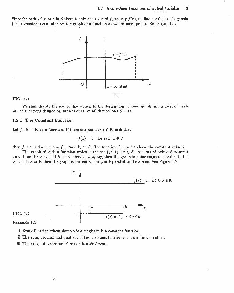
Since for each value of x in S there is only one value of f, namely f (z), no line parallel to the yaxia (i.e. x-constant) can intersect the graph of a'function at two or more points. See Figure 1.1.
FIG. 1.1
We shall devote the rest of this section to the description of some simple and important real- valued functions defined on subsets of R. In all that follows S E R.
1.2.1 The Constan t Funct ion
Let f : S -+ R be a function. If there is a number k E R such that
f (x) = k for each x E S
then f is called a constant function, k, on S. The function f is said to have the constant value k. The graph of such a function which is the set {(x, k) : x E S) consists of points distance k
units from the x-axis. If S is an interval, [a, b] say, then the graph is a line segment parallel to the x-axis. If S = R then the graph is the entire line y = k parallel to the x-axis. See Figure 1.2.
FIG. 1.2 f(x)=-1, a 5 x l b
Remark 1.1
i Every function whose domain is a singleton is a constant function.
ii The sum, product and quotient of two constant functions is a constant function.
iii The range of a constant function is a singleton.

1.2.2 The Identity hnction
The function from R to R whose value a t any z in R is z is called the identity function and is denoted by Id. Thus
Id (z) = z for all z E R.
The domain of Id is R and the range ie R. The graph of the identity function is the straight line 9 = x shown in Figure 1.3.
FIG. 1.3 Identity function
1.2.3 The Signum F'unction
A function from R to R whose value at any z in R is 1, 0 or -1 according to whether z is positive, zero or negative respectively is called the signum fpcnction and is denoted by sgn. Thus
The domain of sgn is R while the range is {-1,0,1). The graph of this function is shown in Figure 1.4.
FIG. 1.4 Signum function

1.2.4 The Heaviside h c t i o n
The function fiom R to R whose value at any positive real number ia 1 and whose value at all other real numbers i 0 ia called the Heaviside function or Heaviside step function. Let w denote it by H. Thus H : R 4 R is given by: For all x in R
The domain of H i R while the range is (0,l). A aketch of this function is ahown in Figure 1.5.
FIG. 1.5 Heaviide function
1.2.5 T h e Modulus or Absolute Value Function
The modulus function or absolute value function on R is denoted by mod and is defined by the following: For all x in R
x i f x > O
-x i f z < O .
Another notation for mod (z) i~ lzl. The symbol 1x1 is read as 'the absolute value of x' or 'the modulus of x' or 'the mod of z'. A sketch of the function mod is given in Figure 1.6.
FIG. 1.6 mod (z) lzl Some properties of the abwlute value function are so important that we list and prove them
in the following.

6 Functions
Result The absolute value function has the f~llowing properties: For all x in R
(1) 1x1 > 0. (ii) 1xI=O if and only if x = 0 .
(iii) 1 - X I = 1x1,
For all x , y in R
Property (iv) is usually referred to as the triangle inequality.
PROOF. If x > 0 then 1x1 = x > 0. If x < 0 then 1x1 = -x > 0. If x = 0 thrn 1x1 = 0. Hence 1x1 3 0 for all x in R. We need to show that 1x1 = 0 + x = 0 and x = 0 + 1x1 = 0. Both of these are immediate consequences of the definition of mod. For x > 0 , -x < 0 therefore I - X I = -(-x) = x = 1x1. For x < 0, -x > 0 therefore I - X I = -x = 1x1. For x = 0 , I - x( = 0 = 1x1. Hence for all x in R I - xl = 1x1. We shall prove this assertion for the various combinations of ranges of values of x and y , For x = 0, x + y = y therefore )x + y( = (yl and 1x1 = 0. Hence lx + yI = 1x1 + lyl. A similar argument holds for y = 0. Now consider the cases when x and y have the same sign. For x > 0 a n d y > 0 , x + y > O a n d s o ( x + y ( = x + y = 1x1 + Iyl. For x < 0 and y < 0, x + y < 0 and so 1x + yI = -(x -t y) = -x + ( - y ) = 1x1 + Iyl. The only case left is when one of the numbers x , y is positive while the other is negative. Let us consider the case x > 0, y < 0. The argument for the case x < 0 , y > 0 is similar. ~ e t -y be denoted by z.
i x - z i f x > z ( x + Y ( = ) x - - z l = 0 i f x = z
z - x i f x < z . Now x > 0 and z > 0. Therefore -z < 0 < z + x - z < x+z and -x < 0 < x + z - x < z + x . Hence ( x + y( < x + z = 1x1 + Izl = 1x1 + I - yl = 1x1 + 191 by (iii). Thus for all combinations of ranges of values of x and y, ) x + y( 5 1x1 + ( y ( . An alternate proof
of part (iv) is suggested in the exercises. 0
Observe that the domain of the absolute value function is R while the range is (0) U R+.
1.2.6 The Greatest Integer Function Given any real number x the set consisting of all integers less than or equal to x is a non-empty subset of R and is bounded above. The number x is an upper bound of this set. Therefore the set has a least upper bound. This least upper bound is called the greatest integer less than or equal to x and is denoted by [ X I . We may therefore define the greatest integer function or largest integer function
[ I : R + R
as follows: For all x in R, [ ] ( x ) s [x] is the largest integer less than or equal to x. For example

1.2 Red-valued Functions of a Real Variable 7
A graph of the largest integer function is shown in Figure 1.7. The domain of [ ] is R while the range is 2.
FIG. 1.7 The greatest integer function
1.2.7 The Linear Function
Let a be any real number. The function f : R + R whose value for any x in R is given by f (x) = ax is called an affine function or a linear function. In this text however we shall follow the convention in such introductory texts to extend the definition of linear function as follows. Let a and b be any real numbers, the function f : R + R whose value for any x in R is given by f (x) = ax + b shall be called a linear function. Thus in our usage here an affine function is a special case of a linear function. As the reader is aware the graph of the affine function y = ax is a line through the origin while that of the linear function y = ax + b is a line that intersects the y-axis a t y = b .
The domain of the affine function is R while the range is R except for the special case a = 0 in which case it is the constant function zero whose range is the singleton (0). Typical graphs of the affine and linear function are shown in Figure 1.8.
a. Affine functions b. Linear functions
FIG. 1.8

8 Functions
1.2.8 The Polynomial Function
Suppose we start with the constant function and the identity function and apply the operations of summation and product to these functions we generate more complex functions. For example the affine function f : R -, R with f (x ) = ax is a product of the constant function g : R -* R, g(x) = a and the identity function Id : R + R with Id (x ) = x. That is f = g - Id. An important clam of functions that may be generated by such operations on the constant function and identity function is the polynomial function. A polynomial function of degree n, denoted by p : R + R say, is given by
p(x) = a n x n + a n - t x n - l + - . . + a 2 x 2 + a l x + a o , n E N
where a,, . . . , a0 are constants. Note that
mfactors - I d . I d . . . Id(x) = xm for any m E N .
The shape of the graph of a polynomial function depends on n and all the constants a,, . . . , ao. We expect that the reader will be in a good position to draw such graphs by the time he or she has completed Chapter 4 of this text. The domain of the polynomial function is R. The range depends on n and the values of a,, . . . , ao.
1.2.9 The Rational Function
Suppose p : R + R and q : R -, R are polynomial functions of degrees n and m respectively and q is not the constant function zero then the function r which is the quotient of p by q is called a rational function. .Thus r : R + R is defined by
where p and q are polynomial functions. The domain of r is R-{x i : q(xi) = 0 ) . The range of r cannot be deterrninec.1 without knowledge of p and q.
1.2.10 The Root Function
Recall that for any non-negative real number a its nth root where n E N is defined as the non- negative number b such that bn = a. I t is usually denoted by f i. If a is a negative number then there is no even nth root of a, that is, there is no real number b such that bn = a for n even and a < 0 . However, there exist odd nth root of a negative number. In fact, if a < 0 and n is odd then the nth root of a is the negative of the nth of -a. That is
6 = -- fl-a) for a < 0, n odd.
Based on the above we define the nth root function as follows; For all x in S 5 R the nth root function is the function whose value is given by fi. For n even S = ( 0 ) U R+ while for n odd S = R. The range of the nth root b c t i o n is ( 0 ) U R+ for n even and R for n odd. Graphs of the

1.3 Real-valued Functions of a Real Variable Q
root function are shown in Figure 1.9 for n = 2 and n = 3.
Y
n = 2 n = 3
FIG. 1.9 nth root function
1.2.11 Trigonometr ic Functions
We ehall assume that the reader is familiar with all the trigonometric funct ionssine, cosine, tangent, eoeecant, secant, cotangent. Here we shall restrict discussions to trigonometric functions on R.
Exercises 1.2
Prove that the product of two constant functions is a constant function.
Find I d sgn (2) and compare it with mod (2).
Determine mod. H(x) and sketch its graph. I d
Is - (2) = mod (x)? Explain. sgn
Draw the graph of f : [O, 16) -, R defined by f (x) = [A. Prove that the sum of two affine functions is an affine function.
Prove that the sum of two linear functions is a linear function.
Express the polynomial function f : R --t R where f (2) = 3x4 - 22 + 1 as a combination of the sums and products of the identity function I d and the constant function k : R -, R where k(x) = k: Prove that the quotient of two nonzero affine functions is a constant function. Is the quotient of two nonzero linear functions a constant function or a linear function or neither? Draw the graph of the functions (i) f (ii) g and (iii) f l g if f , g : R + R are given by f (x) = 2x - 1, g(x) = x + 1. Find dom (f lg) and range (f lg) .
Draw the graph of the rational function r : S -, R where r(z) = 1/x and S = [-4,O) U (0,4]. What is the range of r?
12 This problem concerns an alternative proof of Result (iv) for the absolute value function, that is, Jx+yl 5 It/+ ly[. First prove that 1xI2 = x2. Then prove that for all x , y in R, lxyl = 1x1 Ivl. Finally by jvstifying each of the equalities and the inequality in the statement
conclude the desired result.
1.3 Composition of Real Functions of Real Variables
Consider two real-valued functions of real variables f : R -, R and g : R -. R. If the set range (g) n dorn ( f ) is not empty then we may define the composite off and g or f composition g , denoted by f o g by
f o g = {(x,y) : for some z in range(g)ndom(f ) , ( x , z ) E g and (z ,y ) E f }
Another notbtion for (f o g)(x) which may be more revealing is f(g(x)). Let us consider a few examples.
Example 5
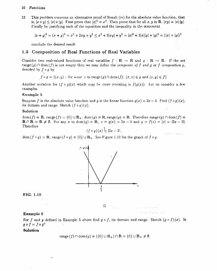
Suppose f is the absolute value function and g is the linear function g(x) = 2x - 3. Find ( f o g ) (x), its domain and range. Sketch (f o g) (x).
Solution
dorn ( f ) = R , range ( f ) = (0) u R + , dorn (g) = R, range (g) = R . Therefore range (g) n dorn ( f ) = R n R = R # 0. For any x in dom(g) = R , z = g(x) = 2x - 3 and y = f (z ) = )z( = (23: - 31. Therefore
( f 0 s ) (8) 1 2 ~ - 31,
dorn (f o g) = R , range (f o g) = (0) U R + . See Figure 1.10 for the graph of f o g.
FIG. 1.10
Example 6
For f and g defined in Example 5 above find g o f , its domain and range. Sketch (g o f ) (x). Is g o f = f o g ?
Solution range ( f ) n dorn (g) = ((0) u R + ) n R = (0) u R+ # 0.

1.3 Composition o f Real Functions o f Real Variables 11
For any z in dom ( f ) = R, z = f ( x ) = 121 and y = g(z) = 2 2 - 3 = 21x1 - 3. Therefore
dom (g o f ) = R, range (g o f ) = [-3, oo) and g o f # f o g. The graph of g o f is shown in Figure 1.11.
FIG. 1.11
Example 7
Draw the graph of the composite function ( H o mod) (I).
Solution
range (mod) n dom (H) = ((0) U R + ) n R = (0) U R +
For any x # 0 in dom(mod) = R , z = mod (x) = 1x1 > 0 and y = H(z) = H(Ix1) = 1. For x = 0 in dom(mod) = R, z = mod (2) = mod (0) = 0 and y = H(z) = H(0) = 0. Thus
( H o mod) ( I ) = { 1 for x # 0 0 f o r x = O .
The sketch of ( H o mod) (x) is shown in Figure 1.12.
FIG. 1.12 (H o mod) ( 2 )

Example 8
Suppose the functions f , g, h : R -, R a r e defined by f (x) = 32 - 5, g(x) = x3, h(x) = ein x. Find
6 ) gob ( 4 g 0 f (iii) h o f
(iv) h o f (v) f o f (vi) h o h
Solution
(i) g o h: Let z = h(x) then (g o h)(x) = g(z). For any x in R , z = sin x and g(z) = z3. - Therefore (g o h) (x) = z3 = (sin x ) ~ = sin3 x.
(ii) - g o f : Let z = f (x) then (g o f)(x) = g(z). For any x in R , z = 32 - 5 and g(z) = z3. Therefore (g o f ) (x) = z3 = (32 - 5)3.
(iii) h o f : Let z = f (x) then ( h o f)(x) = h(z). For any x in R , z = 32 - 5 and h(z) = sinz. - Therefore (h o f ) (x) = sin z = sin(3x - 5).
(iv) - h o g: Let z = g(x) then (h o g)(x) = h(z). For any x in R , z = x3 and h(z) = sinz. Therefore (h o g) (x) = sin z = sin(x3).
(v) - f o f : Let z = f (x) then (f o f)(x) = f(z). For any x in R, z = 32 - 5 and f (z) = 32 - 5. Therefore (f o f ) (x) = 32 - 5 = 3(3x - 5) - 5 = 9x - 20.
(vi) h: Let z = h(x) then (h o h)(x) = h(z). For any x in R , z = sin x and h(z) = sin z. Therefore (h o h) (x) = sin z = sin(sin x).
Exercises 1.3
Problems 1-7 concern the functions f ,g , h : R -, R defined by f (x) = 1x1, g(x) = x+2, h(x) = cosz.
1 Find and sketch the graph of f o g .
2 Find and sketch the graph of g o f .
3 Find h o f .
4 Find f o h.
5 Find and compare f o f with f .
6 Find g o g and compare it with g g.
7 Find h o f and compare it with h. m factora -
8 P r o v e t h a t I d o I d o - . . o I d = I d .
9 I s m o d o H = H ? E x p l a i n .
10 Prove that the composite of two linear functions is a linear function. Is the product of two linear functions a linear function?
11 Prove that for any function f : R -, R, f o I d = f . Is I d o f = f ? Explain.
12 Let f : R + R be defined by f (x) = x2. Show that d o f = mod (2). (In
abbreviated notation this implies that h? = 1x1). 13 Show that mod o sgn = sgn o mod and sketch the graph of either function.
14 Show that J o [ I = [ I for 0 5 x 5 2. Is J o [ I = [ I for all x in (0) U R+?

1.4 The Inverse of a Function
Given a function f the relation consisting'of all ordered pairs that are obtained by interchanging the first and second coordinates of f is called the inverse of the relation f . In general this relation is not a funttion.
For example the inverse of mod is the relation mod-I given by
mod-' : {(x, y) : z = ly(}.
The graph of mod-' is shown in Figure 1.13. Observe that for each value of the first coordinate, with the exception of zero, there correspond two values of the second coordinate. This follows from the fact that (a, -a) E mod-' and (a, a) E mod-' for all a E R.
FIG. 1.13 The relation mod-' = {(z, y) : x = (y()
If how eve^ a function, f say, is one-to-one, that is, for each second coordinate there corresponds only one first coordinate, then the inverse relation f - I is also a function. Under this condition we have the following.
THEOREM 1.1 Iff : R -+ R is a one-to-one function then its inverse f-' : R -r R is also oneto-one and
for all z in dom (f) and dom (f -') respectively.
0
Example 9
Find f-' if f : R -+ R is given by, f (z) = 32 - 4. Verify that Equation (1) is satisfied for all z in R. Sketch the functions f and f-'.
Solution
f ={(z,y) : y = 3 x - 4 ) .
1 4 1 4 y = 32 - 4 =+ z = -y + - Thus f-' T {(y,x) : x = -y + -1. Interchanging the roles of x and y
3 3 ' 3 3 we have
1 4 f - ' = {(x, y) : y = -2 + -1.
3 3

14 Functions
Now 1 4
( j - ' 0 f ) ( x ) = f - ' ( f ( x ) ) = f - ' ( 3 x - 4 ) = - ( 3 x - 4 ) + - = x 3 3
and
The graphs of f and f -' are shown together in Figure 1.14.
FIG. 1.14
Result
Each point ( x o , yo) on the graph of a function and the corresponding point ( y o , x o ) on the inverse function are equidistant from the graph of the line y = x .
PROOF. The distance from a point ( x o , y o ) to a line A x + by + C = 0 is kw. For the line y = x , take
A = 1, B = -1, C = 0. The distance d ( x o , yo) from the point ( x o , yo ) on the graph of the function to the line y = x is j q . The distance d ( y o , x o ) from the point ( y o , x o ) on the graph of the inverse
function to the line y = x is -1. Hence 4 x 0 , Y O ) = YO, l o ) .
Remark 1.2
A consequence of the above result is that the graph of f-' is the 'mirror image' of the graph of f where the 'mirror' is the line y = x .
See Figure 1.14 where the graphs of a function and its inverse are drawn while the graph of the line y = x is shown as dotted line.

1.5 Abbreviated Description of Functions 15
Exercises 1.4
1 Find and sketch the inverse f -L of the affine function f : R -+ R with f (x) = 42.
2 Find and sketch the inverse f- ' of the linear function f : R +'R with f (x ) = i x + 3.
3 Find the inverse f-' of the linear function f : R -+ R with f (x ) = ax + b, a # 0 and b # 0. Verify that (f- ' o f ) (x) = x for all x in R.
4 Find and sketch the inverse f -' of the polynomial function f : R+ + R where f (x) = x2 - 2.
5 Observe that if the domain of s inx is restricted to [-~/2,7r/2] then sin is one-to-one. Sketch the graph of its inverse, sin-' What is the domain of sin-' x?
1.5 Abbreviated Description of Functions
To save time, space and energy, mathematical objects are constantly given abbreviated descriptions or names. Another reason for such abbreviations is that irrelevant detail tends t o detract attention from the main features being discussed. With these goals in mind let us note a few abbreviated descriptions. We shall use the abbreviations to be introduced here in the rest of this text where the emphases will no longer be on the function but on their properties.
Given a non-empty subset S of R, a real-valued function on S is specified by saying 'Let f : S -t R be given by: for all x in S, f (x ) = E(x) ' where E(x) is a mathematical expression. I t is convenient to use the abbreviated forms 'the function x M E(x) ' or 'the function E(x) ' or 'x H E(x) ' or just 'E(x)'. Thus we may talk about the functions x ; 1x1 and 5x + 3 rather than I d ( x ) : R + R , I d ( x ) = x ; mod(+) : R + R , n i o d ( x ) = l x l a n d f : R + R , f ( x ) = 5 x + 3 respectively.
Whenever we use a description like 'the function E(x) ' for a real-valued function the under- stood domain of the function is the non-empty set of all those real numbers a for which E(a ) is a - real number. For example, the understood domains of the functions m,
x respectively [7, m), R - (0) and (-m, O] U (1, w).
Exercises 1.5
Find the understood domain of each of the functions in Problems 1-6.
Miscellaneous Exercises
1 Suppose the functions f , g : R + R are defined by f (x) = ax + b , g(x) = cx + d where a , b, c, d are non-zero constants. Find f + g , fig, g/ f and f . g . Find the domain and range of each.
2 Suppose the functions f , g : R R are defined by f ( x ) = 1 - 4x, g(x) = 1x1 + 2. Find f 0 9 , g o f and gag.
3 Find mod o mod. Is mod o mod = mod? Explain.

4 Determine if the function f : R 4 R defined by f (z) = H(z) + H(-z) ie a conetant function. 5 Find the inverse f-' of the function f : R + R where f (z) = za and verify that f '' o f =
f o f" = Id . 6 Given that the function f : R -+ R is defined by f(z) = z". For what values of n, if any, is
f o f = f . f? For each of these values of n find f o f . Find the understood domain of each of the functions in problem 7-10.
9 4
mod ( 2 ) - 1

Limits and Continuity 2.1 The Concept of a Limit
Calculus provides mathematical tools for studying change. The concept of limit is fundamental in the study of calculus. The idea of limit is a simple one but beginners often have trouble with it. The beginner is, therefore, advised to review this chapter from time to time, if necessary, because it is not possible t o really understand calculus without mastering the concept of limit. To help us understand this concept we begin with a number of illustrative examples.
Example 1
Consider the function f defined by f ( x ) = 4 2 - 1. We construct the following table of values of x close to 1 and the corresponding values f ( x ) (Table 2.1). It is clear from the table that for the given function, when x is a number close to 1 on either side of 1, f ( x ) is a number close to 3. In this way we say roughly speaking that the limit of the function f ( x ) as 2 approaches I is 9.
Table 2.1
Observe that if we had substituted the value 1 for x in the given function f ( x ) = 4 2 - 1, we would have had f ( 1 ) = 4 ( 1 ) - 1 = 3 a t once. We may then rightly ask: why should we go through Table 2.1 to establish that when x takes values close to 1, f ( x ) takes values close to 3 instead of just substituting the value 1 for x in f ( x ) = 4 x - 1 to obtain 3? The following example can throw light on the issue.
Example 2
Let
Table 2.2 x *
x" 1 f ( X I = - x # l 2 - 1 '
x x" 1
. f ( + ) = - x #A x - 1 '
0.8
1.8
0.9
1.9
0.99
1.99
1.001
2.001
0.999
1.999
1.1
2.1
1.01
2.01
1.2
2.3 . .

18 Limits and Continuity
Observe first that f (1) is not defined. Yet we wish to find out what number, if any, f (x) approaches as x approaches 1. From Table 2.2 in which are displayed values of x close to 1 and the corresponding values of f(x) we see that as x approaches 1, f(x) = -, x # 1 approaches 2. The graph of
y = 9, x # 1 is shown in Fig. 2.1.
FIG. 2.1 Again, roughly speaking, we say that the limit of f(x) as x approaches 1 is 2, and write
which is read as " f (x) tends to two as x tends to one"
or equivalently: lim f (x) = 2 or lim,, 1 f (x) = 2 2, 1
read as: "limit of f(x) as x tends to one is two."
The equivalent notation 9 -. 2 as x - 1 is read " approaches 2 as x approaches 1."
0
Example 3
Let f be the function defined by
sin x f (x) = -
x , x # O
where x is measured in radians. We are interested in evaluating lim,,o %. In Table 2.3 are seen values of x and f(x) as x takes values close to zero. It would appear from Table 2,3 that as x approaches 0, f(x) = approaches 1. The graph of is shown in Fig. 2.2.
Table 2.3 t
sin t - 3:
f 0 . 5
0.96
f 0.2
0.994
f 0 . 1
0.998
k0.05
0.9996
f 0.01
0.99998

FIG. 2.2 Notice, however, that f (0 ) does not exist since f (0 ) = = which ie indeterminate.
Example 4
Let
Observe that this fraction is not even defined at x = 0. A table of values of x for x as close to aero as we wieh and the corresponding values of f ( x ) = $ is constructed (Table 2.4).
We see from Table 2.4 that as x takes on arbitrarily small positive values, the corresponding values of f ( x ) = $ increases without bound. Also as x takes on negative values closer and closer to zero, the values of f (2 ) = $ decrease without bound. See Fig. 2.3. So there is no real number that f ( x ) approaches as x gets close to zero.
Y
-2% 5 10
Table 2.4
FIG. 2.3
x 1 - t
x 1 - 2
-10
-0.1
@
lo6
-1.0
-1
-0.1
-10
-0.0001
-10,000
0.0001
10,000
-1O"j
- lo6
-0.01 1 -0.001
1
1
- 100
0.001
1,000
10
0.1
-1,000
0.01
100
0.1
10

20 Limits and Continuity
Exercises 2.1
x i + x - 1 L e t f ( x ) = 2 , x # 1. Make a table of values pf and f (x) taking vdues of z a t
2 - 1 x2 + x -.2
approaches 1. From your table estimate (or guess) lirn 0-1 2 - 1
1-cosx 2 L e t f ( x ) = , x # 0 where x is a real number. Make a table of values of z and f(z)
x 1-cosx
for values of x as x approaches 0. From your table guess the value of lim s-0 x
1-cosx 3 Let f(x) = , x # 0 where x is a real number. Make a table of values of z and f(z)
x2 taking values of x as x approaches 0. F'rom your table guess the value of
1 - cos x lim +-0 x2 -
By making a table of values of x as x approaches xo, or otherwise, determine for each of the problems 4 to 10 below whether f(x) has a limit at xo. Guess lirn,,,, f (x) if it exists.
2.2 Definition of Limit
Recall that the notation 1x1 < 1 means -1 < x < 1 so that if, in particular, we write lx - 41 < 1, this means -1 < x - 4 < 1 which simplifies to 3 < x < 5. Thus, to say that x satisfies the inequality Ix -41 < 1 is'equivalent to saying that x lies between 3 and 5; that is, x lies in the darkened region in Fig. 2.4 which consists of points distant less than 1 unit from 4. Observe that in the shaded region x can take the value 4.
FIG. 2.4: )X - 41 < 1.

2.2 Definition of Limit 21
I f we now modify this inequality and write instead 0 < Ix - 41 < 1, the expression 0 < lx - 41 means, among other things, that x # 4. Thus, the symbolic expression 0 < lx - 41 < 1 means 3 < z < 5 , s # 4. Thus to say that x satisfies 0 < \ z - 41 < 1 means that x lies in the region sketched in Fig. 2.5. Observe that the point x = 4 is deleted from the region. More generally, the statement "For any given positive number, 6,0 < Ix - cl < 6" means that "x can be made as close to c as we please but without its being equal to c." Such an interval may be called a deleted delta neighbourhood of c.
FIG. 2.5: 0 < 1x - 41 < 1.
We are almost ready for a precise definition of what is meant by the statement "a function f of a variable x has a limit L as x approaches a number c." The essence of this concept is that the values, f ( x ) , of the function f are as close to L as we please for all values of the independent variable, z, in a sufficiently small interval about c , x # c. The requirement that z # c is necessary because sometimes f has a limit as x approaches c even though f may not be defined a t c.
We can express this notion of limit by saying that the function f has a limit L as x approaches c if and only if for any positive number E > 0, there is a number 6 > 0 such that I f ( z ) - LI < E
whenever 0 < Iz - C I < 6, Formally, we have the following:
DEFINITION 2.1 Let c be a point in some interval I of the real line R. Let f be a function which w defined at every point of I etcept possibly at c. The l imit o f the funct ion f a s x approaches c is L, written
1im f ( 2 ) = L (or f ( z ) - L as z - c) , 2 - c
if for a n y positive number E (no matter how small) there is some number 6 > 0 such that I f ( 2 ) - LI < E for all 0 < 12. - cl < 6.
It is important to emphasize that in the above definition the number E > 0 is first given. Then we try to find a number 6 > 0 which satisfies the condition of the definition. Suppose we wish to show that lim,,6(3z - 4 ) = 14. Following definition 2.1, let the "any E > 0" be given by E = A, say. Then we want to find a 6 > 0 such that I f ( x ) - 141 = I(3x - 4) - 141 < for all 0 < Ix - 61 < 6. Now I f ( x ) - 141 = 132 - 4 - 141 = 13(x - €91 = 312 - 61. If we now use the condition lx - 61 < 6 we obtain If ( x ) - 141 = 312 - 61 < 36. Since we want 6 > 0 such that ) f (z) - 141 < & we may set 36 = $ and this equation gives us a desired 6 as 6 = &; which completes the verification. Indeed any 6 > 0 such that 36 5 & will do.
If on the other hand we had started with E = 15 say, then from the above calculations we would have had to set 36 5 15 so that in this case 6 5 5. In general, for this problem the desired 6 > 0 is obtained by setting 36 5 E or 6 5 56. Observe therefore that 6 depends on E . Let us write our discussion above more formally in the following.
Example 5
Prove that lim (32: - 4 ) = 14. 2-6

22 Limits and Continuity
Solution
Let E > 0 be given. Our job now is.to find a 6 > 0 ( 6 a function of e) such that for all x satisfying 0 < 1% - 61 < 6 we have I f ( x ) - 141 < E so we compute
Set 36 = E so that 6 = $. Then I f ( x ) - 141 < E which completes the proof.
Example 6
Prove that
0
lim 1x1 = 0 . 1-0
Solution
Given e > 0 we look for a 6 > 0 such that 1x1 < 6 11x1 - 01 < E . NOW 11x1 - 01 = 11x1 1 = 1x1. By selecting 6 = E , we then have that
so that lirn,,~ 1x1 = 0.
Example 7
Prove that 2 + 1 3
lim - = -. 1-2 3 x + 4 10
Solution
Let E > 0 be any given number. We want to find some 6 > 0 such that whenever 0 < ) x - 2 ) < 6 we have that ( f ( x ) - 1 < E .
We compute
x + 1 3 2 - 2 6 I f ( ~ ) - % I = I--Zl= I 1 0 ( 3 ~ + 4 ) 1 < 1 0 ( 3 ~ + 4 1 since Ix - 21 < 6.
Observe that if x is sufficiently near 2 then x is always positive so that 32 + 4 > 4. Thus
1 - 1 1 < - 10132 + 41 - lO(3x + 4 ) 40.
Using this inequality we obtain
Hence if we set 6 = 406 we get ( f ( x ) - & ( < E as desired, This completes the proof.

2.2 Definition of Limit 23
Remark 2.1
In the application of the definition of the limit of a function, whenever E > 0 is given and we are to find some 6 > 0 such that 0 < (x - cJ < 6 implies that ) f (x) - LI < E , the 6 we find must, in general, be found in terms of the given E . Also if we can show that there is no such 6 then we must conclude that the limit does not exist. These ideas are used in Theorem 2.1 and Example 8 that follow.
THEOREM 2.1 If lim,,, f (x) = L (# 0) then there is a deleted neighbourhood of c within which f(x) has the same sign as L.
PROOF. lirn,,, J(x) = L * given any number E > 0, there exists a 6 > 0 such that if 0 < 1x - cl < 6 then I f ( x ) - LI < E. That is,
In particular for L > 0, take E = $L in (*). Then there exists b1 > 0 such that 0 < Ix - cl < bl 1, - + L < f(x) < L + $ L . Thus O < 12-cl < a l * f ( x ) > i L > O . For L < O , t a k e € = - f - L and 1 t,hcre exists b2 > 0 such that 0 < (I - c( < b2 implies that ;L < f (x) < +L. Hence f(x) < zL < 0 for all 0 < )x - c( < 6 2 .
Remark 2.2
If lirn,,, f (x) = 0, f (x) may be zero, positive, or negative or all of these in any deleted neighbour- hood of c.
Example 8
Prove that lim,,o $ does not exist.
Solution
Suppose the limit exists and is L. We consider the 3 possibilities (i) L > 0, (ii) L < 0 and (iii) L = 0. For x > 0, > 0 also and if x < 0,; < 0 also. Therefore since every neighbourhood of zero contains x < 0 and x > 0, f(x) is both positive and negative in such a neighbourhood. Hence by Theorem 2.1 cases (i) and (ii) cannot hold. Consider therefore case (iii) L = 0. Given any E > 0 we wish to show that there does not exist any number 6 > 0 such that 0 < 1x - 01 < 6 implies that 1; - 01 < E; that is, 0 < 1x1 < 6 I;( < E . Suppose there is such a 6 , say 6". Then 141 < E + 1x1 > for all x in 0 < 1x1 < 6". The two inequalities 0 < 1x1 < 6" and 1x1 > are satisfied only for < 1x1 < 6" shaded in Fig. 2.6.
FIG. 2.6: < 1x1 < 6*'. This violates the requirement "for all x in 0 < 1x1 < 6*." Hence no such 6 exists and so case (iii) cannot also hold.

24 Limits and Continuity
Remark 2.3
You may have observed that in Examples 5'to 7 the limits of the given functions have been asserted in the problem. The definition only helped us to prove that the assertions are correct. If, for instance, we have the following problem:
32 - 2 Evaluate lim -.
2-5 x + 7
The definition of the limit of a function will not help us in this problem. In the next section we shall use the definition to establish some theorems on limits that will be useful in the evaluation of limits.
Exercises 2.2
1 Prove that lim (52 + 3 ) = 13. 2-2
2 Prove that lim (22 + 7) = 3. 2- - 2
3x - 4 - -2. 3 Prove that lim - - 2-0 x + 2
22 - 1 4 Prove that lim - - - 0.
2-4 2x + 1
2.3 Some Theorems on Limits
In this section we establish some basic theorems on limits aimed a t enabling us to determine limits when they exist.
THEOREM 2.2 Let f be the constant function defined b y f ( x ) = k where k is a constant. Then for arbitrary number c ,
lim f ( x ) = k . 2-c
(Thus the limit of a constant function is the constant).
PROOF. Let E > 0 be given. We want to find some 6 > 0 such that 0 < Ix - cl < 6 I f ( x ) - kl < E . Now, I f ( x ) - k I = Ik -k I= ~ 0 ~ = O < ~ s i n c e ~ > O . H e n c e J f ( x ) - k J < ~ f o r a l l x s o t h a t a n y 6 > O w o r k s !
THEOREM 2.3 Let f ( x ) = x for a l l x , then
lim f ( x ) = c. Z+ C
PROOF. ' Let E > 0 be given. We want some 6 > 0 such that 0 < 1x - cl < 6 I f ( x ) - C I < E However, If ( x ) - cl = 1x - cl. Using the condition 0 < 1x - cl < 6, we have J f (x) - cl = 1x - cl < 6. Therefore 6 = E gives the result.

2.3 Some Theorems on Limits 25
for c > 0.
PROOF. Let & > 0 be given. We want to find a 6 > 0 such that 0 < lx - cl < 6 --. [fi - fil < E . NOW,
We need now to find a number A independent of x such that .-$& < Alx - cl. This implies that . . Jf + JE > f . Since 6 > 0, then fi+ fi > fi so that A =.& will suffice. Hence
for all 6 < E&.
THEOREM 2.5 a. Let a be any fixed real number. If lim,,, f (x) = L then lim,,, a f (x) = a L .
(i.e., the limit of a constant times a function is the constant times the limit of the function, if this limit exists.)
b. If lirn,,, f (x) = C and lim,,c g(x) = m, then
lim [f (x) + g(x)] = C + m x-C
lim [f (x) - g(x)] = C - m 2-c
(i.e., the limit of the sum (difference) of two functions is the sum (difference) of the limits, if these exist.)
PROOF. We shall prove just the first part of Theorem 2.5b. and leave the proofs of the other parts as an exercise. b. (i): Given that
lim f (x) = t and lim g(x) = m, 2- c Z d C
we need to prove that lirn,,, [f (x) + g(x)] = C + m. For any number 8 > 0 (and hence any number $ > 0) there is a number, 61 say, 61 > 0 such that I f (x) - Cl < 5 whenever 0 < 1x - cl < 61. Similarly for any > 0 there is a number 62 > 0 such that Ig(x) - ml < 5 whenever 0 < 1% - cl < 62. Now
whenever 0 < 1x - cl < rnin(h1, b2). We take 6 = min(61,62). Therefore 0 < lx - cl < 6 * I [f (2) + g(x)] - (C + m) ( < E , as required.

26 Limits and Continuity
Remark 2.4
Observe that in order to end up with I[f(g)+g(z)]-(e+m)i < e weetarted with 5 in the definitions of limits of f(x) aed g ( x ) . This is generally true in the sense that if Ih(z) - LI < LC, k > 0, then using E I = ~ / k in the initial definitions we reduce this to )h(z) - L( < el. So we can still deduce existence of limit from Ih(x) - L1 < kc.
We now give some examples to show how Theorem 2.5 makw it easy to evaluate the limit of any linear function.
Example 9
Evaluate
a. lirn (22 - 7) t-2
b. lirn (az + b). t - r c
Solution
a. lirn (22 - 7) = lirn 22 - lim 7 (Theorem 2.5b.) t-2 z-2 t-2
= 2 l i m x - 7 r + 2
(Theorem 2.6a., 2.2)
z 2(2) - 7 = -3 (Theorem 2.3)
Hence lirn,,a (22 - 7) = -3. b.
lim(ax + b) = lirn ax + lim b (Theorem 2.6b.) 8-e a-e 1-c
= a l i m x + b t - r c
(Theorem 2.5a., 2.2)
= a(c) + b = ac + b (Theorem 2.3)
Therefore lim,,c(ax + b) = ac + b.
0 Remark 2.5
By repeated application Theorem 2.5 can be extended to cover the limit of the sum of any finiie number of functions. Thus we have the following:
lirn fi(x) = ti, i = 1,2, ..., n then lim[fi(x) + f2(2)+ . - ' + fn(f)] = el + L a + . . . + e n . 8 - C 2 - C
We now state the following useful theorem.
THEOREM 2.6 Let lirn,,, f (z ) = e and lim,-, g(x) = m then
lim[f(x)g(x)] = em I- c
1 1 lim-=- if P f O z-c f ( x l e
Example 10

2.3 Some Theorems on Limits 27
Solution 3x2 - 51: + - 3 1im2,2(3x2 - 52 + % - 3)
lirn - - 0-2 4x2+ 52 - 1 lim,,2(4x2 + 5+ - 1)
Example 11
Evaluate a. lim(3x - 4)2 b. lim(3x - 4)(2x2 + 7x + 2),
2- 1 1-3
Solut ion
a. lim(3x - 4)2 = lim(3x - 4)(3x - 4) s-1 2- 1
= [lim (32 - 4)][lim(3x - 4)] 1-1 1-1
= [3(1) - 4][3(1) - 41 = (-I)(-1) = 1.
Hence lim(3x - 4)2 = 1. 2- 1
b. lirn (32 - 4)(2x2 + 72 + 2) = lirn (3, - 4) lirn (2x2 + 72 + 2) 2-3 1-3 0-3
= [3(3) - 4][2(3)2 + 7(3) + 21 = 5(18 + 21 + 2) = 5(41) = 205.
0 R e m a r k 2.6
By repeated application Theorem 2.6 caq be extended to cover the product of any finite number of functions. Thus, we have the following result:
If lirn f i ( r ) = l i , i = 1 , 2 ,..., n then 2 - C
Example 12
Evaluate lirn (3x - 2)16 2--1
Solut ion
lim (32 - 2)16 = lirn (3x - 2)(3x - 2) (3x - 2) x--1 I--l \ .- t
16 factors
= [ lirn (32 - 2)]16 s--1
= [3(-1) - 2]16 = (-5)'' = 516.

28 Limits and Continuity
2.3.1 Limits of Polynomial a n d Rat ional Functions
A special case of Remark 2.6 is the case in which fi(x) = fa(x) = . . . = fn(x) = x. In this case we obtain that
An immediate consequence of Remark 2.5 and the above equation is that for any polynomial function f (x) = a0 + a1 z + . . . + an x" we have
This fact and Theorem 2.6 give us a quick method for computing limits of quotients of poly- nomial functions (i.e., rational functions) which we summarize as follows:
P(X> If f (3) = - where p(+) and q(x) are polynomial functions, then d x )
2 - C
P(') provided q(c) # 0 a. lim f(x) = lim - = - 14C q(x) ~ ( 4
P(C> b. If p(c) = 0 = q(c) then the quotient - is indeterminate. In this case a further simplification 4 c )
of the quotient may be needed before attempting to evaluate the limit (if it exists). q(x)
Example 13
Evaluate 2x2 - 3x + 3 x 2 + x - 2 x2 - 9
a. lim b. lim c. lim-, x--2 x 3 - 2 - 1 1.41 z2-l-3x+ 1 2-3 x - 3
Solution
a. p ( c ) = 2 x 2 - 3 x + 3 , q ( x ) = x 3 - x - 1 . Sop(-2) = 2(-2)2-3(-2)+3 = 8+6+3 = 17 and q(-2) = (-2)3-(-2)-1 = -8+2-1 = -7
2x2 - 32 + 3 p(-2) 17 Hence lim =-- - --
2--2 23 - x - 1 4-2) 7 '
x2 + 2 - 2 p(1) 0 Therefore lirn --- - - = 0.
1-1 x2 + 32 + 1 p(1) - 5 c. p(x) = x2 - 9 and p(3) = 32 - 9 = 9 - 9 = 0
q(x) = x - 3 so that q(3) = 3 - 3 = 0. A further investigation is needed. Thus we have
x2 - 9 lim - = lim
(X - 3 ) ( ~ + 3) 2-3 x - 3 2 4 3 x - 3 7 x # 3 (Why?)
22 -9 Hence lim - - - 6.
2 4 3 2 - 3
2.3 Some Theorems on Limits 29
Whenever the indeterminate case occurs as in Example 13c. above, both p ( x ) and q ( x ) have x - c as a factor. The process of factorization is often simplified by making the substitution x = c+ h where h is the displacement of the point x from c. We must have h -, 0 as x + c and vice versa. Using this method the solution of Example 13c with x = 3 + h becomes:
x2 - 9 - lim ( 3 + h)2 - 9
lim - - 2-3 X - 3 h - + ~ ( 3 + h ) - 3
6h + h2 = lim - = lim(6 + h ) since h # 0 h - 0 h h - 0
THEOREM 2.7 Suppose that lim f ( x ) = C . If n is a positive integer, then z - c
lim = f l= lirn f ( x ) z - c 4 F '
provided that for n even, C > 0 .
. Remark 2.7 I
The requirement that C > 0 if n is even ensures that the nth root function is defined on an open interval about c.
Example 14
Evaluate
a. lim v 2 x 3 - 3 2 - 18 z + 2
b. lirn ~~ 2 4 3
Solution
= C/[ lim ( x 2 - x + l )I3 z-.-2

30 Limits and Continuity
We now end our list of theorems on limits with the 'fallowing important theorem.
THEOREM 2.8 (SANDWICH THOEREM) Suppoae ihai l o r all z # e in an open interval I containing c
9(z) 5 f ( z ) 5 w. If lirn g(x) = lirn h(x) = e then lirn,,, f (x) = e, also.
z-C z- C
Example 15 1
Evaluate lirn (z sin -). z 4 x
Solution
From trigonometry, for all x in the domain of sin (k) , we have Isin $1 5 1 so that
i.e., 1
Ixsin -1 < 121. Z
This inequality clearly implies 1 -1.1 5 zsin - 1zI. x
Identify g(x) = -1~1, h(x) F 1x1 and f (x) = xein $ 1
Then lirn (- 1x1) = 0 = lirn 1x1 so that by the Sandwich Theorem, lim(z sin -) = 0. z-0 z+o 8-0 t
2.3.2 Lirpits of Trigonometric Functions
In this subsection we focus attention on limits of trigonometric functions. Consider a sector POQ of a circle of unit radius with centre at 0 , the origin of co-ordinates. Let OP make an angle x radians (- 3 < x < 5 ) with 0 Q and R be the foot of the perpendicular from P to 0Q (see Fig. 2.7 for positive z). Reuristically we note from the figure thatasz-rO,P- .Q,R-rQsothat lPRl-,O T
and !OR1 -+ 10Q1= 1. Since IPRI = ls int l and o lOQl= cos x then lPRl= 1 ajn zl -+ 0 and lORI = R Q
c o s x - r l aax -+0 . HG. 2.7 ho rn these we expect that
l imsinz=O and l i m c o e t = I . 2-0 z-0

2.3 Some Theorems on Limits 31
We establish these limits formally. We consider AOPQ and sector OPQ whose areas are $Isin X I and 31x1 respectively. Since 0 < aiea of AOPQ 5 area of sector OPQ, we have
But lim,,o 1x1 = 0. Therefore by the Sandwich Theorem lirn,,~ lsinxl = 0. Thus given E > 0, there exists 6 > 0 such that 1x1 < 6 implies that I sin x( < E . With this E > 0,
I sin x - 01 = I sin21 < E for all 1x1 < 6.
Hence lim sin x = 0. 2-0
For the second limit, we start from sin2 x + cos2 x = 1 for all x . Thus cos I = t/-. Therefore
lim cosx = Iim d- = 4- = 1. 0-0 1-0 2-0
The two results lirn sin x = 0 and lirn cos x = 1 r-0 2-0
enable us to determine the limits of all trigonometric functions at arbitrary number, c, in their domain.
in fact, lirn T(x) = T(c) t- C
for all trigonometric functions; that is for T = sine, cosine, tangent, secant, cosecaqt or cotangent. To prove this claim for T = sine, that is
lirn sin x = sin c t - C
we observe that if we let z = c + h then as x -, c, h -, 0. Therefore
lim sin z = lim sin(c + h), 0-c h-0
Now ein(c + h) = sin c cos h + cos c sin h
and thus limsin(c+ h) =since lirn cosh+cosc. limsinh h-0 h+O h+O
= sin c.
Therefore lirn sin x = sin c. a+e
Similarly for T = cosine, that is lirn ccmx = coac. t + e
Note that cos(c + h) = cos c cos h - sin c sin h.
Therefore lirn ccm(c + h) = coe c lim coe h - sin c lirn sin h h-0 h+O h-0
= COBC

32 Limits and Continuity
which implies the desired result. The limits for other trigonometric functions follow from the sine.and cosine limits and the limit
theorems. We conclude this subsection by deriving an important result
sin x lirn - = 1 r-0 X
which will be used later. From Fig. 2.7 where PT is a tangent to the circle at P and for 0 < x < a/2
Area of AOPQ < area of sector OPQ < area of AOPT
That is. 1 1 1 -sin x < -x < - tan x. 2 2 2
Multiplying through by & we have
x 1 I < - < - .
sln x cosx
On inverting the expression we obtain
sin x cos x < - < 1.
x
This inequality also holds for -H < x < 0. Since lim,,o cos x = 1, then by the Sandwich Theorem
(1) sin x
lirn - = 1. r-0 x
Example 16
Prove that
1-cosx lim = 0. 2-0 x
Solution 1 I - b o s x - 2 s i n 2 j x = s i n 5 x 1 - sin -x
x x f x 2
Therefore 1 - cosx sin 4%
lirn 1
= (lim T) (lim sin -2) 2-0 t z-0 p 2'0 2
sin h = ( t m -) ( t m sin h) = (1)(0) = 0 -0 h -0
obtained by replacing i x by h and noting that h = i x + 0 as x + 0.
0 Example 17
x Find lim (z - -)tan z.
2-4 2

2.3 Some Theorems on Limits 33
Solution
Plll 2 = " + h 2 7r 7r h sin(; + h) h cos h
(x - -) tan x = h tank- + h) = - - 2 2 cos(5 + h) - sin h
7r h cos h lim (x - -) tan x = lim (- -
2- 5 2 2 h-o sin h
. h = -(!m -) (lim cos h) -os inh h-o
= - ( l ) ( l ) = -1.
Exercises 2.3
f rove Theorem 2.5a. 1 1
Prove a. lim x2 = c2 b. lim - = - if c # 0. 2 - C 2-c x C
Evaluate each of the limits in problems 3 to 11 stating the limit theorem(s) that apply.
lim (2x2 - 3 x + 1) 2- 2
4
x 2 - - x + 2 lim 2-1 x 3 + x2 - 3
lim (x2 - 2)(x2 + 32 + 1) 2-0
8
x 2 + x - 2 lim
2--2 x2 + 2x
lim 1
w-3 Jw3 - 2w2 + 7
lim (2 - x + x ' ) ~ 2- - 1
lim f ('1 - f(3) for /(XI = JF . 2-3 - 3 Find each of the limits in problems 12-14 where c is any number in the domain of f .
1 lim - for f (x) = - 2-c 2 - c x
lim f -.f for f (x) = JF 2-c x - C Evaluate each of the limits in problems 15-17 below
1 - cos x lim 2-0 x2
csc x - cot x 16 lim
r-0 X
sin x - x cos x lim 2-0 x3
sin kx If k # 0 prove that lim - = k. Is the result true for k = O? Justify your answer.
0-0 x

84 hmits and Continuity
2.4 F'urther Concepts of a Limit
Examine the following example.
Example 18
Let
The function f is sketched in Fig. 2.8.
FIG. 2.8
Table 2.5 x 1 1 . 7 1 1 . 8 1 . 9 1 1 . 9 9 11 .999
f(x) 1 2.7 1 2.8 1 2.9 1 2.99 1 2.999
We want to compute limZez f ( x ) if it exists. In Table 2.5 are shown values of x and f (z ) as x approaches 2. We observe that as x appraoches 2 from the left hand side of 2 (i.e., z takes values 1.7, 1.8, 1.9, 1.99, 1.999, . . . all these numbers being less than 2) the values of f(x) approach 3; whereas as x approaches 2 from the right hand side of 2 (i.e., x takes the values 2.3, 2.2, 2.2, 2.01, 2.001, . . . all these numbers being greater than 2) the values of f(x) approach 7.
Thus the value f(x) approaches as x approaches 2 depends on the side from which z is ap- proaching 2. In this case the two values, 3 and 7, are unequal and we say that lim,,2 f (z ) does not exist,
It is thus revealed in Example 18 that if c is an arbitrary real number (such as 2 in the example) and z approaches c, then the value which a function f of x approaches depends, in general, on whether x is approaching c from the left or from the right of c. This leads to the notion of one-sided limit.

2.4 Further Concepts of a Limit 35
2.4.1 One-sided Limftr
Let c be a red number and let t > c (so that x lies to the right side of c). Then the "right-hand limit" of a function f of z as z approaches c, denoted by
is the number (if any) that f ( z ) approaches as x approaches c. Note that the plus sign (+) which is written as a superscript of c indicates that x approaclies c from the right side. Some texts use the equivalent notation
lirn f (x). +Ic
The "left-hand limit", denoted by lim f ( z ) ,
x-c-
is similarly defined. An alternative hotation is lim,t, f(z). In Example I8 we obtained the following:
lirn j (x) = 3, lim f(x) = 7 c-2- x-2+
and we concluded that since Lim,,2- f(x) # lim,,2+ f(x) , then lim,,z f (x) does not exist. It turns out that this is in general true. In fact, the limit of a function f exists qf and only if ihe left hand limit and ihe righi hand limit both ezist and are equal. Their common value is the limit of the function f ; that is,
lim f(x) = lirn f (z ) = lirn f(+). r-c 2-e+ t‘-c-
Example 19
Consider the function whose graph is sketched in Fig. 2.9. We see that
FIG. 2.9 lim g(z) = lim g(x) = 1
,--2- r--2+
and so the limit of g as x approaches -2 is 1. We write limr,-2g(x) = 1. In this case the two one-sided limits exist and 'are equal.

36 Limits and Continuity
Example 20
Consider the function h sketched in Fig. 2.10.
FIG. 2.10 In this case limr,l- h(z) = -3 but lim,,l+ h(x) does not exist and we conclude that h has
no limit as x approaches 1. In this example the left-hand limit exists but the righ-hand limit does not exist.
Example 21 Consider the greatest integer function f (x) = [x] whose graph is shown in Fig. 1. of Chapter 1. limr,l- [XI = 0 while lim,,l+[x] = 1. In fact, for any integer n,
lirn [XI = n - 1 while lirn [XI = n. r-n- x+n+
Thus f (x) = [x] does not have a limit for any integer value of x.
Example 22
Consider the function f defined by
Find (i) lirn f (x ) and (ii) lirn f(x) . 2-2- 2-2+
Solution
(i) For x < 2, f (x) = 3 - x therefore
lirn f (x) = lirn (3 - x) = lirn 3 - lirn x = 3 - 2 = 1. 2-2- z-2- 2-2- 2-2-

2.4 Further Concepts of a Limit 37
(ii) For x > 2, f (x) = 9 x2 - 4
lirn f (x ) = lim - x-2+ 2-2+ x - 2
= lirn (2 - 2)(x + 2)
2-2+ x - 2 = lirn (x + 2)
1-2+
= lirn x + lirn 2 2-2+ 2-2+
Thus limx,z f (x) does not exist since limZd2- f (x) # limZd2+ f (x).
2.4.2 Limit a t Infinity
Let us now consider limits of functions at infinity. We say that a variable x approaches positive infinity if the variable increases without bound and we write x -+ m. Similarly we say that a variable x approaches negative infinity if it decreases without bound and we write x -, -m. If the value f (2) of a function f approaches a finite value L, say, as x approaches positive infinity, we write
lirn f (x) = L. t-a3
More precisely, we mean by the last equation that given any positive number E , there is some number N such that
I f (x)- L1 < E for all x > N.
The limit as x approaches negative infinity is similarly defined.
Example 23
Prove that 1
lirn (-) = 0. X d o o x
Solution
Let E > 0 be given. We want an N such that 1;) < r whenever x > N. Now ,-$ < E & 1x1 > f Therefore if we take N = $ then x > N a x > i 1x1 > i since x > 0 =+ l i l = ,$, < s.
By a similar analysis to the one in the last example we can show that
1 lirn (-) = 0
2 4 - m z a h .
It can be shown that the results of theorems 2.2, 2.5 and 2.6 a1 o apply t o limits at infinity. We need to replace c in each of these theorems with either oo or . For example, by Theorem 2.6a and Example 23
2 1 1 1
lirn - = l im( - ) . lirn (-)= (O)(O)=O. 2-m 2 2 2-m z zda , x

68 Limits and Continuity
Example 24
3 + x - 2x2 Evaluate lirn
2-m 5 + 22 + 3x2 ' S o h tion We first observe that both the numerator and denominator in the given expression are unbounded as x -, ca. If we divide both numerator and denominator by x2 each of the new expressions becomer, bounded as x -, ca. We can then use the results lirn2,,($) = 0 and lim,,,($) = 0 which we derived above. Thus
3 + x - 2 t a 3 1
lim F + , - 2 = lim r-w 5 + 2 x + 3 x 2 x-a, $ + % + 3
3 - lirnz-m 7 i- lirnzmw $ + limr+w(-2) - ri 2 , by Theorem 2.5b 1im2-m 7 + 1im2-= ; + llm=-,,,, 3
- o + o - 2 - o + o + ~ by Example 23
2.4.3 Infinite Limits
We may also define limits of functions which become uhbounded as the independent variable ap- proaches either a finite number or becomes unbounded. Let us consider the case where the indepen- dent variable approaches a finite number.
DEFINITION The limit of a function f is oo as x approaches a n u d e r c if for any number N there. exists a number 6 > 0 such that f > N whenever Ix - cl < 6 . This limit is denoted b y
lim f (x) = co. 2--c
The following limit lirn f ( x ) = -cw, 2-C
is similarly defined. For the case where the independent variable approaches infinity we have
DEFINITION The limit of a function f is oo as x approaches ca if for any number N there exists a number'M such that f > N whenever x > M and we write
lim f (x) = 00. s-00

2.4 Further Concepts of a Limit 39
Example 25 1
Prove that lim - = oo. r-0 2 2
Soiution 1
For any number N we need to find 6 > 0 such that 1x1 < 6 implies - > N. Now t 2
1 Therefore choose 6 = - then
fl
proving the desired result.
Example 26 1
Prove that lirn - = -00. z-0- 2
Solution
We need to ahow that givkn any number N < 0 there is a number 6 > 0 such that
Since both z and N are negative 1 1 - < N * - < x 2 N
1 - -2 < -- N 1
Therefore c h o m 6 = - - then N
and hence the result foliowe.
0
Exercises ' 2.4
1 In each case (i) - (vi) below determine if the limit exiets and find its value when it exists.
(i) lim egn (2) (ii) lim sgn (z) (iii) lim sgn (x) 0-0- z-o+ z-0
(iv) lim c sgn (2) (v) 1im x agn (2) (vi) L$o sgn (x2). t-O+ z-0-
4- 2 Find lim -.

40 Limits and Continuity
3 Find lim,,o+ f (x), linl,,o- f (x) and lim,,o f (x) if lt exists for
Sketch the graph o f f in the interval -2 < x 5 2.
Find each of the following limits.
1 + x 2 4 lirn -
2-oo 1 - x2
2x2 - 4x + 1 6 lirn
2-oo 3x2 - x + 5
x3 8 lim -
2--co 5x4 + 2
x 10 lirn
,--a ,/=-
1 + x 2 lim -
2--00 1 - x2
x5 - 7x2 + 3 7 lim
1-00 22 - 4 x 5
&
12 Prove that lim - = -m. 2-3- x - 3
x 13 Prove that lim = 00.
1-1+ x 2 + z - 2
2.5 Continuous Functions
In the study of calculus one of the major classes of functions one encounters is the class of continuous functions. In this section we shall introduce continuous functions and study their basic properties. We begin by considering the following example.
Example 27
Evaluate
a. lirn (3x2 - 5x + 7) 1- 2
Solution
a. lim(3x2 - 5z + 7) = 3(2)' - 5(2) + 7 = 9. 2-2
x - 9 b, lim-
x 4 9 & - 3
2 - 9 - lirn lirn - - (x - 9)(& + 3) x-9 fi - 3 2-9 (& - 3r(& + 3)
Notice that the limit of the function f(x) = 3x2 - 52 + 7 as x approaches 2 was found by computing the value of the function a t x = 2 (i.e. by computing f(2)). On the other hand in (b) for the function g(x) = s, g(9) is not even defined. In general, a function f whose limit as x

2.5 Contimous Functions 41
approaches a number c is equal t o f(c) is said t o be continuous at c. More formally we have the following definition.
D E F ~ N ~ T I O N 2.2 A function f is said to be continuous at a point c if and only i f f (x ) exists and
lim f (x) = f (c). 2 - C
Notes
1 From definition 2.2 i t follows that for a function t o be continuous a t x = c, the following three conditions must be satisfied: (i) f must be defined a t z = c (i.e., f (c) must exist);
(ii) lim f (x) must exist; and z+c
(iii) lim f (z) = f ( c ) . x - C
A function f fails t o be continuous a t x = c if any one of the conditions (i)-(iii) fails t o hold. 2 Recall that condition (ii) implies that limz+,+ f (x ) and lim,,,- f (x ) must exist and be equal.
If a function f is not continuous a t x = c, then f is said to be discontinuous a t x = c.
Example 28
Consider the functions f , g, h and k whose graphs are sketched in Fig. 2.11 In Fig, 2 . l l a . we have
lirn f (x) = 5, lim f (x) = 7 x-1- 2 4 1+
and hence limz+l f (x ) does not exist. Consequently condition (ii) is not satisfied so that f is not continuous a t 3: = 1. Observe that condition (i) is easily satisfied here for f(1) = 7.
a. G r a p h o f y = f (x ) b. Graph of y = g(x)

42 Limits and Continuity
C. G r a ~ h of = h ( x ) FIG. 2.11
In Fig. 2.11b, we have:
d. Graph of y = k ( x )
- lim,,, g ( x ) = 5 and g(1) is not defined. Thus condition (i) is not satisfied and g is discontin-
uous at x = 1. For Fig. 2 .11~ . h(1) is not defined so that h is not continuous at x = 1. Finally in Fig. 2.11d.,
limz,l- k ( x ) does not exist so lirn,,l k ( x ) does not exist. Condition (ii) is thus not satisfied so k is discontinuous at x = 1.
Example 29
Determine whether or not each of the given functions is continuous a t the indicated point x = c. x - 25
a, f ( x ) = - c = 25 ,/z- 5' x + 2 X f l
b. g ( x ) = c = 1 -3 x = l
$ ( x - 3 ) x 5 5 c. h ( x ) = { 1
c = 5 r > 5
d. k ( x ) = 3x2 - 52 + 7 , c = -1.
Solution 2 5 - 2 5 0 - - and so f (25) is not defined. Hence f is discontinuous a t x = 25 a. f ( 2 5 ) = - - a - 5 0
b. g(1) = -3 : condition ( i ) holds Also lirn g ( x ) = 3 : condition (i i) holds
z- 1 However lirn g ( x ) = 3 # g(1) = -3. Thus condition (iii) fails and so g is not continuous a t . z-1
x = 1.
c. h ( 5 ) = + ( 5 - 3 ) = 1 , lirn h ( x ) = 1 and lirn h ( x ) = 1.
2-5- z-5+
Thus lirn h ( x ) = 1. Furthermore lirn h ( x ) = h(5) = 1 and so h is continuous a t x = 5. 2-5 r-6
d. k(-1) = 3 ( - 1 ) ~ - 5(-1) + 7 = 15 and lirn k ( z ) = 15 so that k is continuous a t x = -1. z-- 1

2.6 Types of Discontinuities 43
Continui ty on an interval
If a function is continuous at each point of an open interval it is said to be continuous on the interval. The function f is said to be continuous on the closed interval, a 5 x 5 b, if f is continuous at each point of the open interval, a < x < b, and also lim,,,+ f(x) = f (a) and limx,b- f (x) = f(b).
Similarly f is said t o be continuous on the half-open interval a < x < b or a < x 5 b if it is continuous on the corresponding open interval, a < x < b, and limx,,+ f(x) = f (a ) or lim,-*- f (2) = f (b) respectively. Thus f(x) = ,/Z is continuous on 0 5 x < m.
Example 30
d m Determine for which x the function f (2) = - is continuous,
x + 5 Solut ion
The function d n is defined for all values of x satisfying x -3 and x 2 3. However, if x = -5 then x + 5 = 0 and the function f is not defined. Thus, the given function f has domain D given by ( -w, -5) U (-5, -31 U [+3, w ) . Clearly, the function f is discontinuous at x = -5 since f (-5) is not defined. Furthermore,
lim ,/n ,/= = 0 = f(3), and lim - = 0 = f(-3).
s-3+ x + 5 x--3- x + 5
Thus f is continuous on (-oo, -5) U (-5, -31 U [+3, m) its entire domain.
If a function f ie continuous a t x = c, say, its graph must be unbroken a t x = c. Thus the graph of the function which is continuous a t x = c can be drawn past x = c without 'lifting the pencil from the paper'.
2.8 Types of Discontinuities
The graphs of several discontinuous functions are displayed in Fig. 2.11 (Example 26) of Section 2.5. In particular, the graph of Fig. 2.11b. is that of a function continuous everywhere except a t x = 1 where it has a 'hole'. If we plug the hole we have a function that is continuous everywhere. Thus the discontinuity at z = 1 is 'removed'. More formally this plugging of the hole is accomplished by defining a new function, fD(x), which is equal to f(x) everywhere except at x = 1. At this point we set f D ( l ) = 6 = lim,,l f (x). The new function
is continuous everywhere. In general if x = c is not in the domain of f but lim,,, f (x) = L, the domain of f is enlarged
by defining f'(c) = L, and f*(x) = f (x) for all x # c. (2.i)
The reasoning above shows that f. is continuous at x = c. A discontinuity of f which can be removed by extending the domain of definition as above is
called a remotrable discontinuity of f (x).
44 Limits and Continuity
The other discontinuities (Fig. 2.11a., c. and d.) cannot be removed. In the case where lirn,,, f (x) fails to exist, the function f is discontinuous at x = c and the discontinuity cannot be removed. The function is said to have an essential discontinuity a t x = c. However, if lim,,,+ f (x) and lim,,,- f (x) both exist but are not equal, the discontinuity of, f at x = c is called a jump discontinuity. Every jump discontinuity is an essential discontinuity.
Example 31
In each of the following, classify the given point, c, as one of continuity, removable discontinuity, or essential discontinuity. If the discontinuity is removable, define f*(x) (see equation 2.1) and if essential, determine if it is a jump discontinuity.
Solution
1" 6( l ) + 5 0 a. f (c) = f (1) = = - and so f is not defined at x = 1. Hence f is not continuous
1 2 - 4 ( 1 ) + 3 0 a l 2 = 1. However,
x2 - 6% + 5 (x - 1 ) ( ~ - 5) lim f (x) = lim = lim 2-1 2 -1x2-4x+3 z - l ( x - l ) ( x - 3 )
x - 5 -4 = lirn - -- - = 2. t - 1 2 - 3 - 2
Since lim,,, f(x) = lim,,l f (x) exists, the discontinuity of f at x = 1 is removable. If we now define
x2 - 6x + 5 f * ( l ) = 2 and fb(x) =
x 2 - 4 x + 3 ' ~ $ 1
we have lim,,l f'(x) = f'(1) = 2 and so f' is continuous at x = 1.
b. f (3) = 32 + 1 = 10, lirn f(x) = 10, lirn f(x) = 6. Since lirn f (x) $ lirn f(z) we have that a+3+ 2-3- a-3+ 2-3-
lirnzd3 f (x) does not exist and so f has an essential discontinuity at x = 3. Since the left hand and the right hand limits exist (and are unequal) this is a jump discontinuity.
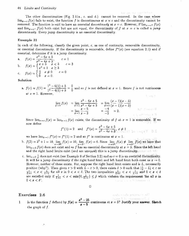
c. limx,o does not exist (see Example 8 of Section 2.2) and so c = 0 is an essential discontinuity. It will be a jump discontinuity if the right hand limit and left hand limit both exist as x + 0. However, neither of these exists. For, suppose the right hand limit exists and is L, necessarily positive (why?). Then given E > 0 with L - E > 0, there exists 6 > 0 such that )$ - LI < E or - <.x < for all x in 0 < x < 6. The two inequalities&% < x < and 0 < x < 6 are satisfied only if < x < min(6, A) 1.6 which violates the requirement 'for all x in 0 < x < 6'.
Exercises 2.6 za - 25
1 Is the function f defined by f(z) = - continuous a t x = 5? Justify your answer. Sketch 2 - 5
the graph of f .
2.7 Some Theorems on Continuity 45
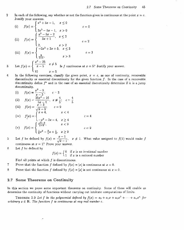
2 In each of the following, say whether or not the function given is continuous a t the point x = c . Justify your answers.
I x 2 + 3 x - 1 , x 5 0 6) f (x) = c = o
3 x 2 - 5 2 - 1 , x > o x2 - 52 - 2
, 2 5 2 c = 2
x > 2 -222 + 32 + 5, x 2 3
(iii) f (x) = c = 3 x > 3
x2 - 25 3 Let f(x) = # is f continuous a t x = 57 Justify your answer.
10 x = 5 4 In the following exercises, classify the given point, x = c , as one of continuity, removable
discontinuity or essential discontinuity for the given function f . In the case of a removable discontinuity define f' and in the case of an essential discontinuity determine if it is a jump discontinuity.
25x2 - 16 (ii) f (x) =
4 4 , x # , 5 ; c = - 52 - 4 5 2 - 3 ,
(iii) f (x) = - 3 c = 9
2 - 1 5 Let f be defined by f(x) = - x # 1. What value assigned to f(1) would make f A- 1 '
continuous at x = I? Prove your answer. 6 Let f be defined by
f c ) = { 0 if x is an irrational number 1 if x is a rational number
Find all points at which f is discontinuous. 7 Prove that the function f defined by f(x) = 1x1 is continuous at x = 0.
8 Prove that the function f defined by f(x) = [XI is not continuous at x = 0.
2.7 Some Theorems on Continuity
In this section we prove some important theorems on continuity. Some of these will enable us determine the continuity of functions without carrying out intricate computations of limits.
THEOREM 2.9 Let f be the polynomial defined by f(x) = ao + a lx + a2x2 + . . . + a,xn for arbitrary x E R. The function f is continuous at any real number c .

46 Limits and Continuity
PROOF, Let c be any real number.
lim f ( x ) = lim(ao + a l x + alx2 + . - + a n t n ) Z'C Z d C
= a0 + alc + a2c2 + . . + ancn
Also f ( c ) = a0 + alc + azca + . - . + ancn. Thus lim,,, f ( x ) = f ( c ) . Hence f is continuous at c.
0
Remark 2.9
Particular polynomials to which the above theorem applies are (i) the constant function f ( z ) = k for all x and (ii) the identity function f ( 2 ) = x for all x .
P ( X ) THEOREM 2.10 Let f ( x ) = - where p and q are polynomialfunctions. Then f is continuous e ( 4
at every point c in its domain, D.
PROOF. Let c be any point in D. From theorems on limits we obtain
P(X) p(c) f ( c ) lim f ( x ) = lim - = - = Z-c z-c d x ) d c )
because c E D q(c) # 0. Thus f is continuous at c.
THEOREM 2.11 The trigonometric functions are continuous in their domains.
PROOF. See subsection 2.3.2 on limits of trigonometric functions.
THEOREM 2.12 Suppose that f and g are continuous at c. Then (i) k f where k is a constant, (ii) f + g and (iii) fg are continuous at c. I f g ( c ) # 0, then (iv) f / g is continuous at c.
PROOF. Since f and g are continuous at c,
lim f ( x ) = f ( c ) and lim g ( x ) = d c ) . X'C x -C
(i) lim [k f ( x ) ] = k lim [ f ( x ) ] = k f ( c ) . Hence k f ( x ) is continuous at c. 2 - C Z'C
(ii) We must show that lim ( f ( x ) + g ( x ) ) = f ( c ) + gtc). Now, lim ( f ( x ) + g ( ~ ) ) = lim f ( x ) + x-C I - C X'C
lim g ( x ) = f ( c ) + g(c) and so f + g is continuous at c. I - C
(iii) By limit theorem
Hence f g is continuous at c.
f ( x ) 1 - f - f ( 1 hr ,(,) # 0. - lim ( f ) ('1 = $Z go - lim.+, g ( x ) g(c) r -c

2.7 Some Theorems on Continuity 47
Thus is continuous at all c E D, its domain. 9
0
Remark 2.10
'I'heorem 2.12 asserts that the sum of continuous functions is a continuous function; the product of continuous functions is also continuous; and the quotient of continuous functions is continuous at all points where the denominator is not zero.
Remark 2.11
It follows from our theorems on limits and Theorem 2.12 that any function f that can be defined by a finite number of some or all the operations of
(i) addition, subtraction (ii) multiplication, division
(iii) raising to powers (iv) extraction of roots
on one or more continuous fun.ctions is continuous at all points in its domain. It then follows that we can find the limit of such a function f at any point c in its domain merely by substituting c for x in f@).
Example 32 Evaluate
5x3 - 72 + 2 a. lim
z--2 t7 + 11
Solution a. The function is continuous a t x = -2. Therefore
5z3 - 7~ + 2 5(-2)3 - 7(-2) + 2 24 lim - - -- -
X--a x7 + 11 (-2)' + 11 117'
b. The function f defined by limx-3 4- is continuous at x = 3, therefore
We conclude this section with the following theorems on the continuity of composite functions.
THEOREM 2.13 Suppose (i) lim,,,g(z) = b and (ii) f is continuous at b, then
lim( f o g)(x) = lim f (g(x)) = f (lim g(x)) . x+c 2-c t - C
PROOF. (f o g)(z) = f (g(x)). Let t be the variable for the fundtion f . f continuous a t b given E > 0, there exists 6i > 0 such that (t - bl < 6i ==+ I f( t ) - f(b)J < e. Also lim,,,g(x) = b implies that given E I > 0, there exists 6a > 0 such that

48 Lirnils and Conlinuity
By taking = 61, g(x) is in the interval it - b( < 61; that is,
Is(+) - bl < 61 * If (s(+)) - bl < E ;
Thus given E > 0, there exists 61 = ~1 and hence 62 > 0 such that
0 < I Z - c( < 62 - Ig(c) - bl < €1 = 61 - I f ( g ( ~ ) ) - bl < E .
Hence
THEOREM 2.14 composite off and g
If (i) g is continuous at c and (ii) f is continuous - is continuous at c.
at g(c), then f o g - the
PROOF. This follows from the proof of Theorem 2.13 above by taking b = g(c) and dropping "0 <" in (*) and (**).
R e m a r k 2.12
A consequence of the above theorem is that a continuous function of a continuous function is con- tinuous. For instance, f (x) = i /5 is continuous a t any point c and g(x) = * is continuous a t any real number c. By the theorem
is continuous a t any x = c,
Intermediate V a l u e T h e o r e m
At the end of Section 2.5 we remarked that the graph of a function is unbroken wherever the function is continuous. In particular, there are no sudden jumps in the values of the function where it is continuous and its graph can be drawn without lifting the pencil from the paper. We now give some mathematical justification for this expression. In fact, if f is a continuous function on [a, b] then f (x ) cannot skip any value, ,Ll say, lying between f (a) and f(b). This is established in the following basic theorem for continuous functions called the Intermediate Value Theorem. We simply state this theorem and omit its proof which is beyond the scope of this book.
THEOREM 2.14 (~[NTERMEDIATE VALUE THOEREM) S U ~ ~ O S ~ (i) f is continuous on [a, b]
(ii> f (a) # f (b) then for any number yl between f (a ) and f(b), there exists at least one X I in (a , b) such that f (xl ) = yl (i.e., f takes on every intermediate value between f (a) and f(b)).
One very useful application of Theorem 2.14 is that i t can be used t o locate intervals containing a root of an equation f (x) = 0, if f is continuous. If [a, b] is an interval such that f ( a ) and f(b)
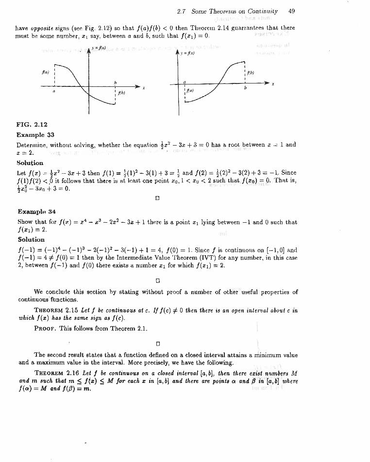
2.7 Some Theorems on Continuity 49
have opposite signs (see Fig. 2.12) so that f(ca)f(b) < 0 then Theorem 2.14 guarrantees that there must be some number, X I say, between a and b, such that f ( x l ) = 0.
y = j w A y =px,
* * ,r
FIG. 2.12
Example 33
Determine, without solving, whether the equation 3x2 - 32 + 3 = 0 has a root between x = 1 and x = 2.
Solution
Let f ( z ) = $x2 - 32 + 3 then f (1) = + ( I ) ~ - 3(1) + 3 = $ and f (2) = b(2)2 - 3(2) + 3 = -1.. Since f (I) f (2) < 0 it follows that there is at least one point xo,1 < zo < 2 such that f (xo) = 0. That is,
- 3x0 4- 3 = 0. 0
Example 34
Show that for f (z) = x4 - z3 - 2z2 - 3x + 1 there is a point XI lying between - 1 and 0 such that f ( 2 l ) = 2. Solution
f (-1) = ( - I ) ~ - (-I)= - 2(-1)2 - 3(-1) + 1 = 4, f (0 ) = 1. Since f is continuous on [ - I , 01 and f (-1) = 4 # f (0 ) = 1 then by the Intermediate Value Theorem (IVT) for any number, in this case 2, between f ( -1) and f ( 0 ) there exists a number X I for which f (21) = 2.
We conclude this section by stating without proof a number of other useful properties of continuous' functions.
THEOREM 2.15 Let f be continuous at c . If f (c) # 0 then there is an open interval about e in which f ( 2 ) has the same sign as f ( c ) .
PROOF. This follows from Theorem 2.1.
The second result states that a function defined on a closed interval attains a minimum value and a maximum value in the interval. More precisely, we have the following.
THEOREM 2.16 Let f be continuous on a closed interval [a,b], then there exist numbers M and m such that m 5 f ( 2 ) 5 M for each 2 in [a, b] and there are points a and 0 in [a, b] where f (m) = M and f ( P ) = m.
50 Limits and Continuity
Exercises 2.7
In questions 1 to 5 say whether or not the given equation has a solution in the given interval. Justify your answers.
1 x a - 2 x + 3 = 0 , [1,2]
2 x 3 - x - 1 = 0 , [O,II
3 x 3 - x - 1 = 0 , [o ,q 4 x 4 - x 3 - 3 x - 2 = 0 , [1,3]
5 x= + x4 - x3 + xZ - x - 1 = 0, [-I, I]
In questions 6 and 7 find an interval containing a root of the given equation
6 2x3 + 3x2 + 62 + 7 = 0
7 23"+1- 4" + 2 .2" - 1 = 0
In the following determine how many roots, if any, of the equation lie in the given interval.
8 4 x 4 - 4 x 3 + x 2 - 4 = 0 , [-1,2]
9 2~~ + x3 + 2x2 + 1 = 0, [-2,2].
Miacallaneous Exercises
1 Prove that lim(3x - 5) = -2. z-rl
x2 - 4 lirn Find (i) z--2 x2 - + - 6 (ii) z-ro lim (mod o H)(x) .
x - 4 x 2 - x - 2 lim - 4 Find (i) z+4 f i - 2 (ii) lim x--1 x2+2a!
3x2 + x - 6 5 Find lim
d 5 - x + 4 x 4 ' In each of the following, say whether or not the given function ie continuous at the point z = c. Justify your aqswer.
f (x) = (H o mod) (x) c = O
Determinie if the equation x3 - x2 - x - 1 = 0 haa a solution in the interval [1,2]. Find an interval containing a root of the equation x3 - 2x2 - x + 17.= 0.

The Derivative
3.1 Introduction
Thie chapter is concerned with the concept of the derivative of a function of one real variable. Consider a function f of a real variable x whose values are denoted by QI = f (x). The quantity x is the independent variable while y is the dependent variable. The derivative which will be defined shortly represents the rate of change of the dependent variable with respect to a change in the independent variable.
Let us discusa two examples. Consider a person running along a straight track. The position of the person ss meesured from any reference point on the track is a function of time, t. We denote this position by s(t). The displacement or net distance the runner travels between two instants t = to and t = t l is s(tl) - 8(to). Therefore the average velocity of the runner in that time interval is
displacement a(tl) - e(to) average velocity = - -
time taken h - to
Obviously if t l = to the above ratio is indeterminate, being g. We may ask the question: With to fized, does the average velocity have a limit as tl approaches to? If the answer to the question ie yes then we call this limit the velocity v(t) of the runner at the instant t = to. It is also called the derivative of the displacement with respect to time. Observe that since this operation can be carried out at different values o f t it determines another function of time.
As another example we consider the graph of a function f denoted by the pairs of values (2, f (x)). Let P(xo, Q I ~ ) be a f ixed point on the curve (see Fig. 3.1).
1 I I * x
0 XO XI
FIG. 3.1 If Q is a neighbouring point with coordinates (XI, yl) then the slope of the secant PQ is given by
y1 - YO f (XI) - f (xo) slope of secant = - = X I - xo 21 - x0

52 T h e Derivative
(Compare this rabio with the average velocity ratio). As the point Q is taken closer and closer to the point P, xl approaches xo and f ( x l ) approaches f ( x o ) . Here again we ask the question: does the slope of the secant have a limit as z l approaches xo? If the answer to the question is yes (as it would appear for the curve sketched in Fig. 3.1) then that limit is the slope of the tangent PT to the curve at the point P. It is also called the derivative of f with respect to x . It is again a function of x .
We shall now define the derivative of a function and discuss how to compute this derived function at any point in an open interval in the domain of the original function.
3.2 The Derivative
Consider a function f : I - R where I is an open interval. Let the value of f at any point x E I be denoted by y = f ( z ) . Let yo = f ( x o ) , for some xo in I. At another value x l = xo + A x of z , the corresponding value yl of y is yl = f ( x l ) = f ( x o + A x ) . We have denoted the change in z , namely x1 - xo by A x . Let us denote the corresponding change in y , namely yl - yo by A y . That is
The limit of the quotient 2 as A x tends lo 0, that is
is the derivative of f ( z ) at xo. More formally we have the following definition,
DEFINITION (THE DERIVATIVE) Let f : I -+ R. The first derivative o f f at z o E I denoted b y f l ( z o ) i s defined b y
f l ( x o ) = lim f ( x o + A x ) - f ( + o ) Az-0 AX
if the limit exists.
0
The first derivative is also called the differential coeScient or simply the derivative. Also the derivative at xo is denoted by any of the following:
When there is no chance of confusion the argument may be omitted and the following notations may be used. .
The quantities f' and $ are read as ' f prime' and 'dy dx' or 'dy by dx ' respectively. There are several alternate ways of representing the definition of the differential coefficient. Observe that if we set x1 = x o + A x then as A x -+ 0, X I - xo . Therefore
D f ( X O ) = lim f (4 - f ( 2 0 ) 2 1 - z o X I - xo

3.2 The Derivative 53
Another notation for the change in x is h rather than Ax. Thus
D f ( x 0 ) = lim f ( x o + h) - f ( X I h - 0 h
As we already observed f ( x O + Ax) - f ( x O ) is the change Ay in y = f ( x ) corresponding to the change Ax in x. T h a t is Ay = f ( x o + Ax) - f(xo). Thus we may write
From these equations we may extract a mnemonic form for the derivative, namely
- d' = lim - AY dx A X + O Ax'
The process of finding the derivative of a function is called differentiation. A function is said to be digerentiable at a point if its derivative exists a t the point. A function
is digerentiable in an open interval if it is differentiable a t every poiht in the interval. If the limit in the definition does not exist at xo, then xo is called a singular point of the
function, Many of the functions we shall be considering have derivatives defined a t all points in their
domain. Thus their derivatives are themselves functions of the independent variable defined in the same domain.
Let us consider a number of examples.
Example 1 Find the rate of change of the area of a circle with respect to the radius.
Solution
Let r be the radius of the circle and A its area, then
Let r(i be any value of the radius. For this A(r0) = nr;. For the increased radius r = ro + Ar the new area is A(r0 + Ar) = n(ro + Ar)2. The corresponding change in the area, AA, is given by
and
= n(2ro + Ar).
Therefore dA . AA - ( P O ) = lim - - dr
- lim n(2r0 + Ar) = 2nr0 Ar+O AP Ar-0
Hence $$ = 2 ~ r , for any r . That is, the rate of change of the area of a circle with respect to the radius has the same value as the circumference of the circle.

54 The Derivative
Example 2
Find the slope of the tangent to the curve y = f ( z ) = 3x2 + 5 a t the point ( x , y) = (-1,8).
Solution
We need to find the limit of the ratio l- as At approaches zero. Now f ( - 1 ) = 8, f (- 1 + AX) = 3(-1 + AX)' + 5 = 8 - 6Ax + AX)^.
Therefore
and dy - = lirn
f ( - 1 + Ax) - f ( - 1 ) dx AX-0 AX
= lim (-6 + 3Ax) = -6. At -0
Thus the slope of the tangent a t (-1,8) is -6.
0
Before proceeding to determine the derivative of several classee of functions such sa the constant function, the identiy function, the power function and the trigonometric functions sine, c a i n e and tangent let us show that every function is continuous wherever it is differentiable.
Result
If a function is differentiable a t a point c then it is continuous there.
PROOF. We wish to prove that lirn f ( x ) = t ( c ) . Now 2 - C
Therefore lirn f ( z ) = f ( c ) and hence f is continuous a t x = c. Q d C
The converse of the above result is not true since a function may be continuous a t a point without being differentiable there. For the example the function f ( x ) = x2I3 is continuous at a = 0 but not differentiable there since
does not exist.
Result
The derivative of the constant function is the zero function.
PROOF. Consider the constant function f ( x ) = k. Let xo be any point in R. f ( x o ) = k , f ( x o + Ax) = k therefore Ay = f ( t o + Ax) - f ( x o ) = k - k = 0. Then
AY 0 lirn -= lirn -= lirn 0 = 0 for a l l x = x o . D f (") = A x 4 0 Ax Ax-0 A+ AX-0

Hence 3.2 The Derivative 55
D f ( z ) = D k = O f o r a l l z ~ R .
Result The derivative of the identity function is the constant function 1.
PROOF. Consider the derivative of the identity function f ( x ) = z at an arbitrary point zo. f (20) = z o , f ( z o + Az) = 20 + A2 therefore
D f ( z ) = Dz = lirn f ( 2 0 + Az) - f ( 2 0 )
Az-O AZ
= lim (20 + Az) - z0 hz-o Az
Since zo is arbitrary the desired result follows.
Example 3 Find the derivative of f ( x ) = fi, z > 0 a t each point in its domain. Solution
= lirn 21 - 2 0
zI-=o (21 - z o ) ( f i + 6)
1 Therefore D f i = -
2 6 '
Let us conc1ud;e thie section by defining the derivative a t an end point of an interval. We define the left-hand derivative of a function f at a point b by
if the limit exiets. Similarly we define the right-hand derivative of f at a point a by

56 The Derivative
if the limit exists. We say that a function is differentiatjle in a closed interval [a, b] if it differentiable on (a, b) and
its right-hand derivative and left-haxid derivatives exist a t a and b respectively.
Example 4
Determine the right-hand derivative of f ( 2 ) = 1x1 at x = 0.
Solution
By definition, the right-hand derivative o f f a t x = 0 is
= lim 2 since I A Z ~ = A2 for A= > o Az-O+ A2
= lim 1=1. Az-rO+
0
Exercises 3.2 Find the derivative of each of the function defined in problems 1-4 below.
1 . f ( 2 ) = x3
5 Find the left-hand derivative of f ( 2 ) = 1x1 at x = 0.
3.3 Derivative of the Power Function
Result (The Integer Power Formula)
For n a positive integer, the differential coefficient of x" is nxn-'
PROOF. Denote the function by f with f ( x ) = x" and let xo b,e any point in R. f ( z 0 ) = xg , f ( x o + A x ) = ( x o + A x ) " . From the binomial theorem (see, for example, Equation 2 of Section 4.4 of Volume 1)
Therefore
A f = ( x o + Ax)" - xg = Az [ (;) + (;) X ; - ~ A X + - - - + (:) ( A Z ) ~ - ' ]
From this it follows that

3.3 Derivative of the Power Function 57
'Therefore
The above result may -be generalized for arbitrary power function, that is for f ( x ) = xA where X is any real number.
Result (The Power Formula)
DX' = AxA-', x # 0 for all A E R.
PROOF. We observe that for xo # 0 as A x tends to zero IAxl < 1x01. Also we can write
A x (xo + A)* = x i ( 1 + ;)'.
.. . . > , . sincezr& 1 < 1 expanding (1 + %)' by the binomial expaniorl (see, for example, Eq. (3) of Section
4.5 of 'Volume 1). We have
= x'; + ( A x ) b x ; - l + + . + X(A - 1 ) . . . (A - k + 1) x ~ - k ( A x ) k - l + . . .
k! 0
Hence
and therefore
( X O + A)' - 2; A- 1 + A(A - x;-2Ax + . . , = Axo
A x 2!
lim ( zo + A)' - x; = AX;-' Az-o AX
(4) DX' = AX'- ' , x # o for all x E R.
0 Example 5
Find the first derivative of each of the functions defined below.
(i) f ( x ) = x6 1
(ii) f ( x ) = - 23' x # O
( i i f (2) = GI x > 0

58 The Derivative
(i) From the result (3) n = 6 and hence -&x6 = 6x5
( i i ) Here, X = -3 since 5 = x - ~ and by (4)
(iii) Noting that f i = x f we substitute f for X in (4) to get
( iv) In this case we take X = - $ since & = & = =-'I7. Therefore
(v) Again this is a special case of (4) with X = R. Therefore
DzU = nx"-l.
0
Exerqises 3.3 Determine the first derivative of each of the functions in problems 1-7.
3.4 Derivatives of Trigonometric Functions
We now consider the differentiation of the trigonometric function sine, cosine and tangent.
Result
The first derivative of sin x with respect to x is cosx.
PROOF. Let f(x) = sinx and xo be any real number. Then by the use of the identity sin(A + B) = sin Acos B + cos Asin B we have
j (x0 + Ax) - f (XO) = sin(xo + Az) - sin(xo) = sin xo cos Ax + cos xo sin Ax - sin xo = sin xo(cos Ax - 1) + cos xo sin Ax

3.4 Derivatives of Tkigonornetric Functions 59
Therefore
cos(Ax) - 1 sin Ax = sin xo . lim + cos xo . lim -
at-o A2 At-o Ax = sin x0 . 0 + cos to . 1 (see Subsection 2.3.2)
= Cot3 20
Since xo is arbitrary it follows that
( 5 ) D s i n x = c o s x fora l lx .
Reeult 0
The first derivative of cos x with respect to x is -sin x ,
PROOF. Let y = f (x) = cosx and xo be any real number. Then
Ay = f(x0 + Ax) - f (xo) = cos(x0 + AX) - cos(x0).
Recall that cos A - cos B = -2 sin 9 sin 9 (see, Subsection 5,6.2 of Volume 1). Therefore Ax Ax
Ay = cos(xo + Ax) - cos(xo) = -2sin(xo + -)sin 2
and d(cos x) . AY -(xo) = lim -
d~ As--0 Ax -2 sin(xo + %) sin 9
= lim As-0 AX
Ax A2 sin = - lim sin(xo + -) . lim -
AZ-0 2 A s 4 0 k 2
which gives the desired result
(6) D cos x = - sin x for all x .
Prove the above result by applying the identity cos(A + B) = cos A cos B - sin A sin B.
Result
The derivative of tan x is sec2 x,
PROOF. Let f (x) = tan x and let xo be a real number in the domain of f .
f (xo + Ax) - f (xo) = tan(x0 + Ax) - tan io
- tan 20 + tan Ax - - tan xo 1 - tan xo tan Ax
- tan zo + tan Ax - tan xo(l - tan xo tan Ax) - 1 - tan xo tan Ax
- - tan Ax(1 + tan2 xo) 1 - tan t o tan Ax
- - tan Ax sec2 xo 1 - tan zo tan Ax

60 The Derivative
Therefore
D f ( x o ) = lim f ( x o + A x ) - f ( 2 0 )
Az-0 AX tan A x sec2 xo
= lirn AZ-o A x ( 1 - tan xo tan A x )
sin A x = sec2 2 0 . lim - . 1
lim - . lim 1
A=-o A x A Z - o cos A x A=-0 1 - tan x o tan AX
From this it follows that
(7) D tan x = sec2 x for all x in the domain of tan x .
0
Exercises 3.4
Determine from the definition the derivative of each of the functions in problems 1-4.
1 f (x ) = secx
2 f (x) = cscx
3 f ( x ) = sin(ax) where a is any real number.
4 f ( x ) = cos(ax) where a is any real number.
3.5 Rules of Differentiation
In this section we establish a number of results that will enable us determine the derivative of sums, products and quotients of functions of a single independent variable.
The results to be derived in this section are so inter-related that it is pedagogically inefficient to treat many examples and exercises a t the end of each result. We shall treat a minimal number of examples at the end of each subsection and collect all the exercises at the end of the section.
We start by considering the derivative of a sum of two functions of a real variable.
3.5.1 Derivative of a Sum or Difference of Functions
Result Suppose f and g are functions which are differentiable at some number xo . Then
PROOF. Let y = ( f + g ) ( x ) = f ( x ) + g ( x ) be the sum of the functions f and g .

3.5 Rules of Differentiation 6 1
from which we have
Therefore
or equivalently ( f + g) ' (xo) = f l ( x o ) + g l ( x o ) .
R e m a r k 3.1
From the above result it follows from the distributive law that if D f i ( x o ) exists for i = 1 , 2 , . . , n then
for any finite number n. The functions are all evaluated at xo.
Example 6
Let f be a function defined by f ( x ) = x2 + 5 , x # 0. Find f ' ( x ) and determine where it vanishes.
Solut ion 2 1 f ( x ) = x + -.
x2
BY (8) 1
f l ( x ) s o f ( . ) = 0 ( x 2 ) + D c a )
= 2 ~ - 2 ~ 4 by (4).
Suppose f' vanishes a t X O then
3.5.2 Derivative of the P r o d u c t of a Cons tan t and a Function
Resul t
Suppose k is the constant function and f is differentiable a t some number s o then
( 1 0 ) D { k f ( z ) ) = k D f ( z ) for k constant.

62 The Derivative
PROOF. Let y ( x ) = k f ( x ) then
Therefore AY - = k . f ( x + A z ) - f ( z ) A x A x
We take the limit of each side of the equation as A x -+ 0 to obtain
or D{k f ( 2 ) ) = kD f ( x ) for constant k.
Note that in the proof of the last result we have dropped our pedantic scheme of first of all deriving the derivative at some arbitrary point zo and then restating the result by replacing zo by 2. Henceforth we shall obtain derivatives at an arbitrary point z .
Example 7
Find the derivative of ( 2 2 - Solution
Let h(x ) = ( 2 x - 1)' then
h ( x ) = ( 2 ~ ) ~ + 3 ( 2 ~ ) ~ ( - 1 ) + 3 ( 2 ~ ) ( - 1 ) ~ + ( - I ) ~ by the Binomial Theorem
= 8z3 - 12x2 + 6 x - 1.
Therefore
In Section 3.6 we shall discuss an alternative and more efficied method of obtaining derivatives of functions such ae the one in the last example. You may readily observe that h ( x ) = ( 2 x - may be rewritten as the function f ( u ) = u3 of a function u = g ( x ) = 2x - 1.

3.5 Rules of Differentiation 63
3.5.3 Derivative of the Product of Functions
Let us now consider a generalization of the result in the last subsection to the case where neither of' the product functions is the constant function.
Result (Product Rule) Let u and v be two functions which are differentiable at x , then
D(uv)(x) = u(x )Dv(x ) + v (x )Du(x ) or more concisely
( 1 lc) (uv)' = uv' + u'v.
PROOF. Let f (z) = U ( X ) v ( x ) then
f ( x + A x ) - f ( x ) = u(x + 4 x ) v ( x + A x ) - u(x )v (x ) = u(x + Ax)v (x + A x ) - u(x + A x ) v ( x ) + u(x + A x ) v ( x ) - u(x )v (x )
= U ( X + A x ) [ ~ ( x + A x ) - v(x)] + ~ ( x ) [u(x + A x ) - u(x)] . Therefore
v(x + A x ) - v ( x ) At-0 AX AX
v(x + A x ) V ( X ) U ( X + A x ) - U ( X ) = lim u(x + A x ) . lim + v (x ) a lim At-0 An-0 AX At-0 AX
which is the desired result.
0
Remark 3.2
In the proof above we could have added and subtracted the quantity u(x)v(x + A x ) rather than u(x + Ax)v (x ) . The final result would be the same. Try it.
Remark 3.3
An alternative proof of the last result would be to introduce changes in u and v as follows:
A u = u(x + A x ) - u ( x ) a u(x + A x ) = u ( x ) + A u
Av = V ( X + A x ) - v ( x ) =j v (x + A x ) = v ( x ) + Av.

64 The Derivative
Then A f = f (i + A,x) - f ( x )
= U ( X + A X ) V ( X + A x ) - u(x )v (x )
= ( u ( x ) + A x ) ( v ( x ) + A x ) - U ( X ) V ( X )
= u(x )Av + v ( 2 ) A u + AuAv.
Therefore A f Av Au A u - A x = u(x)- A x + ~ ( 2 ) - + -Av. A x A x
Now take the limit as A x + 0 observing that as A x + 0, 4 D f ( x ) , 2 + Du(x) , + Dv(x) and Av -* 0. Therefore
D f ( x ) = u ( x ) Dv(x) + v ( x ) Du(x)
as before.
Remark 3.4
The above result can be extended to the product of a finite number of functions by its repeated application. Thus, let the functions f i , i = 1,2, . . . , n be functions that are differentiable a t some number x , then
In each of the terms on the right only one of the functions f , , f 2 , . . . , fn in the product is differentiated and there is no repetition. Each function is evaluated at the same value x.
For the special case f l = f i = f3 = . . - = f,, = f , say,
D ( f ... f ) = D f . fn - '+ ...+ D f . f n - l . * ' " /
n terms n terms
That is
which is a generalization of the Integer Power Formula.
Example 8
Find the derivative of x2 sin x.
Solution
Let f ( 2 ) = x2 sin x. We identify the functions
2 U = X , v = s i n x .
Then applying (11) we have
D (x2 sinx) = uDv + vDu
= x20s in x + sin XDX'
= x2 cos x + 2x sin x.

3.5 Rules of Differentiation 65
Example 9
Find the derivative of (22 - I ) ~ .
Solution
We identify the functions f l = f 2 = f3 = f with 22 - 1 in Remark 3.4. Then setting n = 3 in the result D f n = n fn" D f in that Remark we have
Compare this solution with that of Example 7. 0
3.5.4 Derivative of a Quotient o f T w o F'unctions
We conclude the section by considering the derivative of a quotient of two functions.
Result (Quot ien t R u l e )
Let u and v be two functions which are differentiable at a number x with v ( x ) # 0, then
or more concisely,
vu' - uv' ( ) I = v2 .
PROOF. 1 1
Let us first of all consider the derivative of -. Let g = -, then v v
1 1 - -=- v (x + A x ) - v ( x ) g(x + A x ) - g(x) =
V ( X + A x ) V ( C ) v ( x )v (x + A x ) '
Therefore
4' + AX) - id21 = 1 v (x + A x ) - v(x) D d z ) = di20 A x A x .
1 = --. 1 v ( x + A x ) - v ( x ) lim lim
V ( X ) A=-0 V ( X $ AX) As-0 A X

66 The Derivative
Now by the Product Rule
which is the desired result.
0
Remark 3.5
A common error occurs in the use of (14b,) when students interchange the order of uv' and vu'. A simple way of remembering which comes first is to set v 3 1 in your formula and ensure that it gives u' . Example 10
Use the Quotient Rule to derive D tan x.
Solution sin x
Since tan x = - , we let u = sin x and v = cos x. Then by (14) cos x
- cos X(COS x) - sin x( - sin x) - cos2 x
0
Example 11
Find the derivative of sec x, csc x and cot x.
Solution 1 1 sin x
By(14) Dsecx=D-=-- DCOSZ = - - - sec x tan x. Therefore C.m 1! c082 x cos2 x
(16) Gsecx = secxtanx.

3.5 Rules of Differeritiation 67
(17)
Finally by (15)
Example 12
i 1 D c s c x = D- =-- D sin x
sinx sin2 x - COS x - --
sin2 x = - csc x cot 2.
Dcsc x = - csc x cot x.
x - 1 Find the derivative of - x + 1 '
Solution
D cot x = - csc2 2 .
0
By the Quotient Rule
- , - x + 1 - ( x - 1 )
(x +
since D(x - 1) = 1 and D(x + 1) = 1
Example 13 ,
Find the derivative of sin7 x cos x.
Solution By the Product Rule
sin^ x cos x) = sin7 z D cos x + cos x D sin7 x. I
Now to obtain Dain7x we observe that it is of the form (13) where f(x) =s in+ and n = 7. Thus

68 The Derivative
It follows then that
D(sin7xcosx) = s i n 7 x ~ ~ ~ ~ x + ~ o s x ~ 7 s i n 6 x ~ ~ s i n x
= sin7 x(- sin x) + cos x . 7 sin6 x c w x
= - sin8 x + 7 sin6 x cos2 x
Exercises 3.5
Determine the first derivative of each of the functions in problems 1-30. The quantities a and b are constants and n is a positive integer.
1 1 2+-$. 2 2 0
sin x 25 r
4 xsinx
1 6 -
CSC x
10 t a n x s i n x
14 1 + t a n x 1 - t a n x
18 x(x + l ) (x + 2)(x + 3)
20 (x2 -'q6
1 22 (i) sin x cos x (ii) - sin 2x
2
30 (i) cos2 x - sin2 x (ii) cos 2x

3.6 The Chain Rule 69
3.6 The Chain Rule
Let us conclude our discussion of rules of differentiation with the differentiation of composite func- tions, that is, functions of functions of one variable. The reader may wish to review the discussion of composite function in Chapter 1.
Result (The Chain Rule)
Let f be a function of a variable u differelltiable at some number uo and u be a nonconstant function of a variable x differentiable a t xo with u(xo) = uo. Then the function (f o u ) ( x ) f ( u ( x ) ) is differentiable at xo and its derivative with respect to x a t xo is given by
Alternative notations for the Chain Rule (19) are
where the specific reference to the points xo and uo are omitted as aide-&moire in recalling the essence of the Chain Rule.
Now Au = u(xo + At.) - u(xo) and that implies that u(xo + A x ) = ~ ( x o ) + Au = uo + Au. Note that Au # 0 in general since u is a nonconstant function. Therefore
Also as A x + 0, u(x0 + A x ) + u(xo) and consequently Au + 0. Thus from (*)
= lim f ( U O + Au) - f (uo) , lim U ( X O + A x ) - ~ ( x o ) AU-o AU AZ-o A X

70 The Derivative
Remark 3.6
Note that Equation (13) is a special case of the Chain Rule. If we set f = un in (20a) then Dun = Duun Du = nun" Du.
Example 14 Find the derivative of (22 - I ) ~ .
Solution Let u = 22 - 1 and f ( u ) = u3 then b y (20a)
0 Example 15
Find the differential coefficient of (1 4 x2)2 with respect to x.
Solution Let u = 1 + xZ and f ( u ) = u2 then b y (20b)
or l e t , (1 + +2)2 2 1 + 2z2 + x4. Therefore
or let f ( x ) = (1 + x2)2 = (1 + x2)(1 + x2) then
f l ( x ) = ( 1 + x 2 ) 0 ( 1 + x 2 ) + ( 1 + x 2 ) 0 ( 1 + x2 ) by Product Rule
= 2x(1+ x 2 ) + 2x(1+ x2 )
= 4x(1+ x2) .
In many problems in differentiation there is usually more than one rule that we can use. We encourage you to use the simplest and most convenient rule.
Example 16 Find the derivative of sin(x2 + 32 - 1).

- 3.6 The Chain Rule 71 ~oiution .. .
Let u = z2 + 32 - 1 and f (u) = sin u then f (u(x)) L. sin(x2 + 3x - 1). Therefore
D, f = D, f . D,u
= D, sin u D,(x' + 32 - 1)
= cos u . (2x + 3)
= (22 + 3) cos(x2 + 32 - 1).
Example 17
Find the first derivative of (1 + x3)4 sec(5x + 2).
Solution
The given function may be considered as a product of the two functions (1 + x3)4 and sec(5x + 2). By the Product Rule (11)
We therefore need to determine D, sec(5x + 2) and D,(1+ x ~ ) ~ . For D,sec(5z + 2), let u = 5% + 2 and f (u) = sec u. Then
Ds ~ 4 5 % + 2) = Duf (u) . D ~ u = D, sec u . D,(5x + 2) = s e c u t a n u - 5
= 5 sec(6x + 2) tan(5x + 9).
For D,(1+ xV4, let v = 1 + x3 and g(u) = v4. Then
D,(1+ x3)4 = DVg(v) Dsv
= D ~ V ~ . Dz(l+ x3)
= 4v3 . 3x2
= 12x2(l + x ~ ) ~ . ' - I+
Therefore
With experience based on solving many problems the reader should be able to arrive at Eque tion (*) aa a first step in the solution!
Exercises 3.6 . ,
Find the derivative with respect to x of each of the functions defined in problems 1-14.
1 (3x+4)& 2 (1 -

72 The Derivative
1 9 (z2+; - tan 2 ~ ) ~
4 sin3(l + 4x2)
6 sin v- 8 (3 sin 2x + cos 7x) lo
12 tan(sinz)
14 sin [sin(sin z)]
3.7 Implicit Differentiation
It is sometimes the case that the dependent variable, y say, cannot be explicitly expressed am a function of the independent variable, z say, as in all the examples and exercises that we have eo far treated in this Chapter. For example, in the following relations
and sin(xy) + 2xy2 = 2,
the quantity y cannot be solved for explicitly to give a unique function of z. In fact some relationships may not define any function at all. An example is the relationship x2 + y2 + 4 = 0. Where such relationships define y as a function of x in some interval we shall call such functions implicit functions.
Let us consider the first two of the three relations above. For x2 + y2 = 4, we may write
Y = { d for 0 < x < 2 -4- for - 2 < x < O
Each of the three expressions above defines y as a function of x qnd the pair of values of x and y satisfy. the relation x2 + y2 = 4. There are infinitely many such functions. In all these cases we can readily determine that at any point (x, y) = (xo, yo), where the derivative exists
Show this for any one of the three expressions. For x3 + xy + y5 - 11 = 0 we observe that if x = 2 then one possible value of y is 1. We
therefore expect that for values of x in some neighbourhood of x = 2, values of y also exist. (Ae examples for x = 2.01, y = 0.9809 and for x = 1.98, y = 1.035 to four significant figures). There ie a theorem beyond the scope of this text (callcd the Implicit Fuliction Theorem) which assurea us that

3.7 Implicit Differentiation 73
under certain conditions such a relation defines y as a function of x in some neighbourhood of the point (x, y) = (2 , l ) .
Our interest here is in the much simpler problem of determining 2 for such functions at points where the derivative exists. We proceed by assuming that the derivative exists and apply the rules of differentiation.
Example 18
dl/ Find - at (x, y) = (2, l ) if x3 + xy + y5 - 11 = 0. dx
Soh tion We take the derivative with respect to x of each of the terms in the equation. Thus
Now d d dy d
-(x3) = 3x2, - (xy) = z - + y -(x) by Product Rule (11) dz dx dz dz
and d
dy by Chain Rule (20) z ( ~ ' ) = 5y4&
Therefore /
The process we have just carried out is called implicit digwentiation. Solving for $ gives
and at (x, y) = (2 , l )
0 Example 19
b u r n i n g that the equation sin(zy) + 2xy2 = 27r defines y implicitly as a function of x in some paighbourhood of the point (x, y) = (7r, 1) find D, y at this point.
Solution
W differentiate the equation sin(xy) + 2zy2 = 27r implicitly with respect to x. Thus

74 The Derivative
dY Collecting terms containing - together gives dx
Therefore dY Yc~(xY)+2Y2 - = - dx xcos(xy) + 4xy
which at (x, y) = (n, 1) becomes
dy 1 cos n + 2(1)2 - = - 1 = -- dx ncosn+4n( l ) 37r'
Example 20
Find y1 wherever the relation (x + 4 ~ ) ~ + x2 - 2y7 = 88 defines y as a function of X.
Solution
We take derivative of the given equation with respect to x.
Exercises 3.7 In each of problems 1-5 find y' a t the indicated points in whose neighbourhood the equations prescribe y as a function of x.
1 y5 + 4xy3 + x3 + 1 = 0, (2, y) = (0, -1) 2 2 x 3 + y 3 - x y + l = O , (x1 Y) = (-11 1)
3 tan ny - y - x2 = 0, (x, y) = (d$2, 114)
1 1 1 1 5 5 x s i n ( * y ) + ~ - x 2 = 0 ( x , ~ ) = ( - ~ , ~ ) a n d ( l , ~ ) .
In problems 6-11 find D,y assuming that corresponding functions are defined by the relations,
6 ax2 + bxy + cy2 + dx + ey + f = 0, a , b, . . . , f are constants
7 xy5 - t 2 y + 52 - 3 = 0

3.8 Derivatives of Functions Expressed Parametrically 75
3.8 Derivatives of Functions Expressed Parametrically
Sometimes it is more convenient to relate variables, z and y say, through a third variable. The third variable is usually called a pammeter. For example, we know that the pair of points ( x , y) satisfying the equation
:+ (21) x2 + y2 = 4
describe a circle but this equation does not uniquely define y as a function of x. For, given a value of z , z = 1 say, there are two possible values of y, namely 4 or -&. Consider however the following representation
We can readily observe that z2 + Y2 = (2c0s t )~ + 2sint)= = 4. Thus all the pairs of values of (x, y ) given by (21) lie on the same circle (21). In fact all the points on the circle (21) are also represented by (22) for some value of the parameter of the parameter t . Specifically the two points (1, &) and (1, -A) mentioned above correspond t o t r 5 and t = respectively. There are other parametric representations of (21). Another one is
What are the values of t9 that correspond to the points (I,&) and (1, -a)? We observe that all the functions defined by y = f (x) may also be represented parametrically
simply by setting z = t
Y = f ( t )
since the combination yield$ y = f (t(x)) = f(x). More generally relationships between two variables x and y may be represented in the para-
metric form
where f and g are functions of the common parameter 1. If we wish to treat y as a function of z then f must not be the constant function. For i f f is the constant function, k say, then we have
and this pair of equations gives different values of y for one value of x. Our interest here is to determine the rate of change of y with respect to x (i.e. 2) from the
representation (23).

76 The Derivative
Let to be a point in I and to + At a neighbouring point also in I. Then
Therefore
= lim dto + At) - dto) lim At ~ t - o At at-0 f ( t o + At) - f (to)
For any arbitrary point t we then have
Example 21
Given that x = 2cost y = 2 sin t } 0 j t < 2 r
dy find - and compute its value for t = 9. dx
Solution
0 Example 22
Given that
find D,y for all t .
Solution
BY (24)

3.8 Derivatives of Fhctions Expressed Parametrically 77
Note that
Example 23
Given that the relations
define y as a function of x , determine Dxy as a function of t , x and y and compute its value at (1, x , Y) = $1. Solution
Differentiate each equation implicitly with respect to t . The result is
Therefore
Exercises 3.8
d y 1 Find - i f x = t 2 - 1 and y = t 2 + t . dx d y 2 Find-ifx=sinOandy=OcosO. dx d y 3 Find - .if x = a cos3 O and y = a sin3 0 where a is a constant. dx
d y 4 ~ i v e n t h a t x = u ~ + l a n d ~ = u ~ + u f i n d - . dx
d y t 5 Find - if x = 2 + t 2 and y = - dx 2 + t 2 .
d y 6 Given that x = 2 cos C + cos 2t and y = 2 sin t - sin 21 find - in terms of t and compute its T
dx value for t = -.
2

78 The Derivative
3.9 Higher Order Derivatives
We observed that, in general, the derivative of a function f is aleo a function defined in some s u k t of the domain of f . For example, for f ( z ) = sin z , D f = cos t and both of these functions have the same domain, that is the set of all real numbers. For
' for z > 0 f ( X I = 1.1. D f ( 2 ) = { for < 0 9
so that while the domain of f is all real numbers, i.e., (-00, oo), the domain of D f is (-00, O)U(O, 00). We may then define the derivative D ( D f ) of the derived function Df in the same manner as that of f . Thus
D ( D f ) ( t ) = lim D f ( 2 + A t ) - D f (2 )
Ax-0 A t if the limit exists. This limit is called the second derivative of f with respect to t and is denoted by
Higher order derivatives of f are similarly defined. Thus
D3 f = D(D2 f ) and Dn f = D(Dn-' f ) for any integer n 2 2.
Example 24
Find the second and third derivatives of f ( t ) = t3 + sin z .
Solution
Df = D(z3 + sin z ) = 3 t 2 + cost .
The second derivative is
D2 f = D ( D f ) = D(3t2 + cost ) = 62 - sin t .
The third derivative is D3 f = D(D2 f ) = D(6t - sin t ) = 6 - cost .
Example 25 1
Find D4f if f = -. Z
Solution
f = 3 D f = D(x-l) = z -'. ~~f = D ( D ~ ) = D ( - ~ z - ~ ) = ( - 1 ) ( - 2 ) t - ~ = 2 ~ - ~
-'. D3 f = D(D2 f ) = 2D(te3) = 2 ( - 3 ) ~ - ~ = - 6 ~ - ~ -4 - -'. D4 f = D(D3 f ) = -6D(z ) - -6(-4)t-' = 24tm6.

3.9 Higher Order Derivatives 79
Example 26
If y = coax prove that yy" - ( Y ' ) ~ + 1 = 0 .
Solution
Therefore yyll - (v1)2 + 1 = cos x ( - cos x ) - (sin 2)' + 1
Example 27
Find D,y and ~ z y on any open interval where the relation 4x2 - y2 - 16 = 0 defines y as a function of 2.
Solution
We differentiate the given relation implicitly with respect to x .
Differentiating again with respect to z gives
- 64 - -- since y2 - 4x2 = -16. y3
0 Example 28
Given that the relation y 6 + 3 x y + 2 x 3 + 2 = 0 defines y as a function of z at the point ( x , jr) = ( 1 , - 1 ) find y l ( l ) and y"(1). '
Solution
We are given that y5 + ~ X Y + 2~~ + 2 = 0,
Differentiating implicitly with respect to z gives

80 The Derivative
(ii)
dy We may either differentiate the expression (ii) for - again with respect to x or differentiate (i) dx
implicitly again. We choose to do the latter. Before doing so we observe that
dy dY d2y is the derivative of a product of Y4 and - and that the derivative of - with respect to x is - dx dx dx2
d d while -(y4) = 4 y 3 2 . Therefore
dx
dx dx'
Similar reasoning would apply to the differentiation of other terms in (i). Therefore, differentiating (i) implicitly with respect to x, we have
dY dY dy Note that the first 3- arises from differentiation of 3x- while the second 3- arises from differ- dx dx dx
d' y entiation of 3y. Solving for - gives
dx2
From (ii)
From (iii) and (iv)
d2 Y Try obtaining - by differentiating (ii). dx2
0
Example 29
d2y Find a formula for - if dx2
d2y and use your formula to determine - for the special case x = sin t, y = t cos t . dx2
(iii)
(i.1

3.9 Higher Order Derivatives 81
Solution dy dyldt g' (24) - = - = - Therefore dx dxldt f'
For the specific case f (t) = sin t, g(t) = t cost, g' = cost - t sin t and f' = cost Therefore
dy g' cos t - t sin t -- - - = = 1 - t t a n t dx f' cos t
and d2y $ ( I - t t a n t ) t a n t + t s e c 2 t - - - - - = - sec2 t(sint + t sect). dx2 - cos t cos t
Leibniz's Rule
We conclude this section by stating and proving Leibniz's rule for the nth derivative of a product of two functions.
Result (Leibniz's Rule) Let n 2 1 be any integer. Suppose that u and v are function whose mth derivatives (rn = 1,2, . . . ,n) all exist, then
PROOF. We shall prove this result by employing the Sec. 1.3.1 of Volume 1).
Let P(n) be the statement (25).
P ( l ) is true since
Principle of Mathematical Induction (see for example,
D(uv) = Du v + uDv.
Suppose P(k) is true for k an integer, that is

82 The Derivative
then we want to prove that P(k + 1 ) is true.
Now k ! k ! + (:) + ( r : 1 ) = T!(& - r)! ( r + l ) ! (k - r - I ) !
= k! + r!(k - r)! ( r + l )!(k - r - I ) !
r + l + k - r = k !
( r + l ) ! (k - r)!
- - (k + I ) ! ( r + l )!(k - r)!
and note that (;) = 1 . Therefore
Thus P(k + 1 ) is true. Therefore, by the Principle of Mathemtical Induction P(n) is true for all n.
0 Example 30
1 +,x Find D3 (-) 1 - 2 . Solution
Let u = 1 + x and v = ( 1 - x ) - ' .

Therefore
3.9 Higher Order Derivatives 83
Example 31
Suppme the function u(x) has derivatives of orders up to m at z = 0 show that for f(x) = xmu(x),
Dmf(0)=m!u(O) for m s n . Solution
Let v(x) = zm then
D ~ V = m(m - l)(m - 2) .,(m - k + l ) ~ ~ - ~ , . . . for all k < m and Dm" = m!
Therefore Dkv(0) = 0 for all k < m. By Leibniz's rule
Exercises 3.9
In problems 1-6 find the first and second derivatives of each of the functions with respect t o x (a and b are constants).
4 sin(ax + b) 5 (ax + b)" 6 (x2 + 3)4
7 Find the fourth derivative of y = cos(ax + b) with respect to x where a and b are constants.
8 Find the third derivative of tan(x2 + 1) with respect to x.
dy d2y In problems 9-12 find - and - if the given relations represent y as a function of x (a and dx dx2
b are constants).

The Derivative
d2 Y I f y =3sin2x+7cos2xshow that - + 4 y = 0 . dx2
If y = sec x, prove that y~ = dx
d2y dy 1 If y = d x + d m , prove that (1 + x2)- + x- - -y = 0,
dx2 dx 4
d2y In each of problems 16-19 find - dx2 '
x = 3 + 2 s i n t 17 x = u t
y = 4 - 2cost 1
y = ut - -gt2, u, u and g are constants 2
Find D2 (x COB x).
d2y Find - if y = x2(2 - x ) ~ . dx2
Find D3[x(4 - 2 ~ ) ~ ] .
Find D3(x2 sin x).
Find D3(sin2 x cos 8).
Find the fifth derivative of x5(l + x ) ~ .
Find the fourth derivative of each of the functions (1 - x ) ~ ( I + x ) ~ and (1 - x ' ) ~ . Compare your results and the amount of effort involved in each method. Suppose the function u(x) has derivatives of orders up to n a t a point a and u(a) # 0, show that if f (2) = (x - Q ) ~ U ( X ) then D~ f (a) = 0 for k < rn and Dn f (a) = n!u(a).
Miecellaneous Exercises
Use the definition of the derivative to find the first derivative of each of the functions in problem 1-3.
1 3x2 2 x3I2 3 sin2x
Find the derivative of each of the following functions.
7 (3x4 + 5)6 8 sin2(7x) 9 cos(sin x) -
Assuming that the relations in problems 10-13 define y implicitly as a function o f t find y' in each case.
10 y2 + 3xy + 2x2 - 2x + 1 = 0
11 y 2 x + x 2 Y + 2 7 = ~
12 x s i n y + y c o s x = 2

3.9 Higher Order Derivatives 85
13 y3 - xy = 5x2 + 1.
dy 14 Find - in terms of x and y if x = 3 cos 0, y I= 4 sin 0 . dx dy 15 Find - if x = tZ + 1, y = ts. dx
17 Show that the function y = A sin(ax + b) where A, a and b are constants satisfies the equation d2y 2 s + a y = o .
Find the indicated higher order derivatives in problems 18-20.
18 D ~ [ ( ~ x + q 3 ( x - 4)4] 19 D2(x tanx) 20 D3[(5 - 3 ~ ) ~ ( 4 x - 1)" ].

Applications of the Derivative
4.1 Elementary Applications to Geometry and Mechanics
4.1.1 Tangents and Normals
Recall that in Chapter 3 we established that the slope of the tangent to the graph of a function f(z) at a point (xo, f (xo)) is the derivative fl(xo) of the function at the point. Let us use this result to find equations of tangents and normals to graphs of some functions.
Example 1
Find the equation of the tangent to the curve y = f(t) = a x 2 + 1 a t the points (-1,514) and (0,l).
Solut ion 1 1
fl(x) = -x. Therefore fl(-1) = -- and fl(0) = 0. We shall use the equation of a line passing 2 2
through (xo, yo) with slope m in the form y - yo = m(x - xo). At the point (-1,514) the equation of the tangent is
The equation of the tangent a t (0,l) is
The function and the tangents are graphed in Figure 4.1.
FIG. 4.1

4.1 Elementary Applications to Geometry and Mechanics 87
The normal to a curve at a point P(zo, yo) is the line through P that is perpendicular to the tangent at P.
Since the product of the slopes of two perpendicular lines is -1 and if the slope of the tangent at P is m # 0, then the slope of the normal at P is -l/m.
Example 2
Find the point of intersection of the normals to the curve y = 1 z+; at the points (4,;) and (1,2).
Solution
To determine the point of intersection we need to know the equations of the normals at the given points.
3
Therefore (i) = -3 and yl(l)= 0.
The slope of the normal at (i, q ) is 5 and so the equation of the normal is
The slope of the tangent at (1,2j is 0. Therefore the tangent is parallel to the y-axis. Consequently the normal is parallel to the z-axis. The normal to the curve at (1,2) has equation z = 1. The point of intersection of the two normals satisfies these equations. Solving these simultaneously we get the point (2, y) = (1, $). See Figure 4.2
FIG. 4.2
0 Example 3
Find the equations of the tangent and the normal to the curve 9z2 - 4y2 = 108 at the point (4,3).
Solution The equation of the curve may be written as
Differentiating implicitly we have 18x - 8yy' = 0 from which it follows that

88 Applications o f the Derivative
At the point (4,3), y1(4) = 3. Thus the slope of the tangent is 3 and the slope of the normal is therefore - 4. Consequently the equation' of the tangent at the point (4,3) is
y - 3 = 3 ( x - 4 ) or y = 3 x - 9
and the equation of the normal at the point (4,3) is
1 y - 3 = - - (2 - 4) or x + 3y = 13.
3
These are shown in Figure 4.3. Y
FIG. 4.3
4.1.2 Velocity and Acceleration
If a point object is moving along a straight line its distance, s , from a fixed point on the line is a function of time t . If the function s(t) is differentiable at t = to then the derivative sl(to) is the velocity, v(to) of the object at time to. If v is differentiable a t to (i.e., s(t) has a second derivative at to) then vl(to) = sl1(to) is called the acceleration of the object at time to and is ¬ed by a(to).
Example 4
The displacement of a particle thrown vertically upwards is given by s(t) = 11 + 101 - t2.
(i) Find the velocity and the acceleration at time t = 3.
(ii) At what time is the velocity zero?
(iii) At what height from its initial position does it start descending?
(iv) When does it reach the ground (s = O)?
Solution
s t ) 11+10t-t2 sl(t) = 10-21 sl1(t) = -2. Therefore at 1 = 3, s'(3) = 4 and sI1(3) = -2. The velo.city at t = 3 is 4 while the acceleration is -2. v(t) = 0 implies 10 - 21 = 0, i.e. t = 5. The highest point is reached when the velocity is zero, i.e., a t t = 5. At this time the height is given by s(5) = 36. The initial position is at t = 0, i.e., s = 11. Therefore the height above the initial point is 4 5 ) - 11 = 25. The particle is on the ground when s = 0, i.e., 11 + 101 - t2 = 0. Factoring and solving gives t = -1 or 11. Therefore the particle reaches the ground a t t = .11.
0

4.1 Elementary Applications to Geometry and Mechanics 89
Example 5 . . .-
If the velocity of a particle varies inversely & the square root of the distance traveled, prove that the acceleration varies as the fourth power of the velocity.
Solut ion
Let s be the distance traveled, v the velocity and a the acceleration.
Therefore
Then
v = - - - s 2 where k is a constant. 6
-312 - - - [ ( v since 8 = (;)-'
2
Hence a cx v4.
Exercises 4.1 0
Tangents and Normals
1 Find the equation of a line that is tangent to the curve y = x3 and is parallel to the line 3 2 - y + l = O .
2 Find the equation of the line that is tangent to the curve y = I/+ and is parallel to the line x + 2 y - 6 = 0 .
3 Two lines through the point (1, -3) are tangent to the curve y = xa. Find the equations of these two lines and make a sketch t o verify your results.
4 There are two tangent lines to the curve y = 42 - x2 that pass through the point (2,5). Find the equations of these two lines and make a sketch to verify your results.
In each of problems 5-10, find the slope of the line tangent to the graph of the given functions a t the given points. Also find the equation of the tangent at the point.
5 y = 3x2+ 1, .(1,4) 6 = x3+ 1, (-1,O)

90 Applications of the Derivative
Find the inclination to the x-axis of the tangent to the curve a t the given point in problems 11-13.
2 7r 3 13 y = sin x at (5, --).
In problems 14-16 find the equations of the tangents and normals to the curves.
14 y = 2 x 2 - 4 x + 5 a t ( 3 , I l ) .
15 x2 + y2 = 20 at (-4, -2).
16 x2 + y2 - 4x - 2y + 1 = 0 at (2, -1). 17 Find the equation of the tangent to the curve y(x2 + y2) = ax2 at any point ( z o , ~ ) . The
quantity a is a constant.
Velocity and Acceleration
A point moves so that its displacement s is given by s = 16 + 481 - t3, when and where will it stop and reverse its direction of motion? A point moves in a straight line so that its distance s from the origin at time t is given by the equation s = 5 + 4 sin 21 + 3 cos Pi. Prove that
(i) its acceleration varies as its distance from a fixed point in the line of motion (ii) its motion is oscillatory, and
(iii) the origin is at one extremity of its path.
If s ( l ) = -16t2 + 1001 +400 represents the position of a moving object, find the initial velocity.
a. Complete the table where v is the velocity and a is the acceleration. b. Draw a diagram to describe the motion of the particle. c. If the velocity v ( t ) and the acceleration a(t) have the same sign, what observation can
be made about the speed of the particle? d. If v(t) and a ( t ) have opposite signs, what observation can be made about the speed of
the particle?
Repeat Problem 21 using the position equation s(t) = t2 - 61 + 9.
The position of a projectile P shot directly upwards from the surface of the earth is s = 1171 - 9.8t2.
(i) What is the initial velocity of the projectile. (ii) Find the average velocity over the interval from t = 5 to t = 10 seconds.
(iii) Find the instantaneous velocity a t t = 5 and t = 10 secs. (iv) Find the maximum height reached by the projectile.
If the distance traveled varies as the square root of the time, prove that th& acceleration varies as the cube of the velocity.
If s = 2t3 + 2t2 + 4t - 20, make a table giving the position; velocity and acceleration initially and after 1, 2, 5 and 10 seconds. Repeat Problem 25 for s = 10 cos $2 + 20 sin %t .
Given the position equation s(t) = i3 - 3t2 + 4 and the table t
44 v(t) a( t>
0 2.0 0.5 2.5 1 .O 1.5 3.0 3.5 4.0

4.2 Maxima and Minima 91
A ball is thrown and follows a path described by y = x - 0.02x2 a. Sketch a graph of the path. b. Find the total horizontal distance the ball was thrown. c. For what x-value does the ball reach its maximum height? (Use symmetry of the path). d. Find the equation that gives the instantaneous rate of change in the height of the ball
with respect to the horizontal change and evaluate this equation a t x = 0,10,25,30,50. e. What is the instantaneous rate of change of the height when the ball reaches its maximum
height?
The path of a projectile thrown at an angle of 45' with level ground is given by y = x - $x2 where the initial velocity is vo ms-' .
a. Sketch the path followed by the projectile. b. Find the x-coordinate of the point where the projectile strikes the ground. Use the
symmetry of the path off the projectile to locate the abscissa of the point where the projectile reaches its maximum height.
c. What is the instantaneous rate of change of the height when the projectile is at its maximum height?
Maxima and Minima
4.2.1 Rolle's and the Mean Value Thoerems
Quite often it is important to determine the largest and least values of functions. For example, every businessman would want to minimize costs and maximize profits. A pedestrian walking from point A to point B may want to take the path of shortest distance. A welder may wish to design a water tank of capacity 500 gallops using the minimum amount of materials. By proper representation of these quantities as functions these problems can be formulated as problems of determining the maximum or minimum values of functions.
A function is said to have a relative rnaximum at a point c if the value of the function at c, called the relative maximum value, is greater than its value a t all points close to c. More formally, let f be a function defined in an interval I. The function f is said to have a local or relative maximum a t a point c interior to I if there exists a number 6 > 0 such that f(c) 2 f(x) for all x in I such that 1x - C I < 6, that is c - 6 < x < c + 6. The point (c, f (c)) is called a relative maximam point of the function.
Similarly a function is said to have a local or relative minimum at a point c interior to I if there exists 6 > 0 such that f (c) f (x) for all x in I with Ix - cl < 6 (see Fig. 4.4).
A relative maximum or a relative minimum point is called a relative extremum point. This relative extremum occurs for some value of x, namely x = c. Such a point c in the domain I of f is called a critical point of the function. The relative extremum point of the function is the point (c, f(c)). A point a t which f' = 0 is called a stationary point of f .
v t
a. Relative maximum
FIG. 4.4 A h ,
b. Relative minimum

YZ Appllcatlons of the Derivative
THEOREM 4.1 If a function f defined on an tniemal I has an exiremum ai an inierior point c, and f is differentiable at c then fl(c) = 0 .
PROOF. Let us prove this for the case where c is a relative minimum. There is a 6 > 0 such that f(x) 2 f (c), for Ja - cl < 6. Consider the quotient 9. Now
lim f(x) - f ( 4 = fl(c) x-rc Z - C
which exists. Therefore
lim f ( 4 - f ( 4 = ,im f ( 4 - f(c) = fyC). z+c+ x - C t + c - x-C
Since f (x) 2 f (c), for x > c in the heighbourhood of c
(') - 2 0 and therefore lim f (3) - f (c) = f ~ ( ~ ) 2 0, x - C z+c+ x - C
Also for x < c in the Cneighbourhood of c
('I - < 0 and therefore lirn (') - = fl(c) 5 0. x-C t - r c - x - C
( ii)
F'rom (i) and (ii) it follows that fl(c) = 0.
The case for relative maximum is similar and is left as an exercise.
Note that fl(c) = 0 does not imply that c is a local extremum point. For example consider f (x) = x3.
Note also that f must be differentiable at c, a local extremum, for the vanishing of the deriva- tive. For example x = 0 is a local extremum (minimum) of f(x) = Ixl, however f'(0) # 0, in fact fl(0) does not exist.
If a differentiable function has the same value at two distinct points then it must have a t least one relative extremum between the two points. See Figure 4.5.
FIG. 4.5 At such local extremum c, f1 = 0. This is the essence of Rolle's Theorem which we now state,

4.2 Maxima and Minima 93
THEOREM 4.2 (ROLLE'S THEOREM) Let the function f be continuous on the closed interval [a,b], dlflerentiable in the open interval ( a , b ) , and f ( a ) = f(b). Then there is at least one point c in ( a , b) such that f '(c) = 0 .
PROOF. By Theorem 2.16 of Section 2.7, since f is continuous, it must have a maximum and a minimum on [a, b]. Case 1: f a constant.
If f is a constant then f' = 0 for all x . Therefore pick c as any point in ( a , b). Case 2: f not a constant.
If f is not a constant, then the maximum or minimum is an interior point c, say. At such a point f' = 0 by Theorem 4.1.
Observe that if both maximum and minimum were end points, since f ( a ) = f (b) , it means that f is constant. A contradiction.
Example 6
Determine if each of the following satisfy the conditions of Rolle's Theorem. Where i t does, find all the possible extremum values. If not, give the condition that is not satisfied.
(ii) f ( x ) = x2 + 21, -2 5 x 5 0
(iii) f ( ) , - 1 < x < 1
(iv) f ( x ) = x 2 , 1 5 x 2 2 (v) f ( x ) = 2 3 - 2 , -1 < x 5 1.
Solution
(i) f is differentiable on ( 0 , l ) . f l ( x ) = 1, f ( 0 ) = f (1) = 0. However f is not continuous at x = 1 since lim,,l- x = 1 # f ( 1 ) .
(ii) f ( x ) = x2 + 22, -2 5 x 5 0. f is continuous on [-2,0] and f ( -2) = f ( 0 ) = 0. f l ( x ) = 2 x + 2 = 0 implies that x = -1.
(iii) f ( x ) = 1x1, -1 5 x < 1. f is continuous on [ - I , 1). f (- 1) = f ( 1 ) = 1. However f l ( c ) does not exist at x = 0. So f is not dimerentiable on (- 1 , l ) .
(iv) f ( x ) = x 2 , 1 5 x 5 2. f is continuous on [1,2], differentiable on (1,2) but f ( 1 ) # f (2 ) .
(v) f ( x ) = x3 - x , - 1 < x 5 1. f is continuous on [- 1,1], differentiable on (- 1 , l ) and f (-1) = f ( 1 ) = 0 , f l ( x ) = 3r2 - 1 = 0 implies that x = f f i / 3 .
Let us now apply Rolle's Theorem to derive a very important result known as Mean Value Theorem. This theorem is used frequently in mathematics in proving other theorems. Geometrically it states that given the graph of a differentiable function between two points A and B there exists a t least a point on the graph between A and B a t which the slope of the tangent is equal to the slope of the line segment AB. In 17iq. 4.6a C is such a point while in Fig. 4.6b the points C I , Ca are

94 Applications of the Derivative
such points.
FIG. 4.6
More formally we have the following theorem.
THEOREM 4.3 (THE MEAN VALUE THEOREM) Let f be continuous pn [a, b] and diffel-entiable in (a , b) then there exists at least a point c in (a, b) such that
PROOF. We may apply Rolle's Theorem to prove this result by constructing a fupction F related to f that satisfies Rolle's Theorem. One such function F is
Observe that F(a) = F(b) = f(a). Since f is continuous on [a, b] and differentiable in (a, b) so is F. Therefore by Rolle's Theorem there exists at least one point c in (a, b) such that F1(c) = 0. But
F1(c) = fl(c) - f (b) - f (a) b - a *
Therefore
0 Example 7
Determine if each of the following functions satisfy the conditions o f the Mean Value Theorem. Where the function does find all the possible points. If not give a condition not satisfied.
(i) f ( x ) = 2 - 3 x 2 , O s x < 1,
(ii) f (x) ='x3 - 3x2 - x + 3, -2 5 x 5 3, (iii) f(x) = 4x2f3, -1 5 2 5 27.
Solution
(i) f(x) = 2 - 3x2, 0 , s 1: 5 1. f is continuous on [0, 11, differentiable on (0 , l ) and

4.2 Maxima and minim^ 95
We need to solve f f ( c ) = -6c = -3 which gives c = which is in ( 0 , l ) .
(ii) f ( x ) = x3 - 3x2 - x + 3 , -2 < x < 3. f is continuous on [-2,3], differentiable on ( -2 ,3 ) . f t ( x ) = 3x2 - 62 - 1 and
f ( 3 ) - f (-21,- 0 - (-15) = 3.. 3 - ( -2) - 5
We need to solve f l (c) = 3c2 - 6c - 1 = 3 that is 3c2 - 6c - 4 = 0. Therefore
Both values of c lie in (-2,3).
(iii) f ( x ) = 4x213, -1 s x 5 27. f is continuous on [-1,271. f l ( x ) = $ x - ' / ~ which is not defined for x = 0. Therefore f is not differentiable on (-1,27) Hence the Mean Value Theorem does not apply. Observe that in the last case a not-too-careful student may proceed to compute a number c
such that f l ( c ) = ( f (b) - f ( a ) ) / ( b - a ) and obtain
i.e.,
It ie however to b f (b ) - f ( a ) d ~oted that getting a number c satisfying f l ( c ) = ---- b - a
the Mean Value Theorem is applicable.
oes n lot mean that
We shall now derive two useful applications of the Mean Value Theorem.. One of these es- tablishes the condition for a function to be increasing or decreasing over an interval and the other establishes that two functions with the same derivative differ oilly by a constant.
4.2.2 Monotonicity of a Function
A function f is said to be increasing on an interval I if
for every pair of points X I , 2 2 in I such that 2 2 > x i . Similarly a function f is said to be decreasing on an interval I if
for every pair of points X I , , 2 2 in I such that 2 2 > X I .
If a function is either increasing on an interval I or decreasing on an interval I , the function is said to be monotone on the interval.
Consider a differentiable function f on an interval with ft > 0 everywhere on the interval and let X I , x2 be any two points in the interval. Then the Mean Value Theorem is satisfied on ( X I , 2 2 )
and consequently there exists a point c in the interval such that

96 Applications of the Derivative
1.e.) f ( x 2 ) - f ( x i ) = f1(c)(x2 - 2 1 ) .
If x 2 > x 1 then since f t ( c ) > 0 it follows that f ( x 2 ) > f ( x 1 ) . We have just proved part (i) of the following result.
THEOREM 4.4 Let f be diflerentiable on the open interval I ( i ) i f f' > 0 on I then f is an increasing function on I,
( i i ) i f f ' < 0 on I then f is a decreasing function on I.
Example 8
Determine the intervals in which the function f ( x ) = 2x3 + 3x2 - 12x + 1 is strictly monotone.
Solution
We wish to determine intervals on which f' > 0 or f' < 0
Observe that f 1 > O for x < - 2 and x > l
while f l < O for - 2 < x < 1 .
Thus f is increasing on (-00, -2) and ( 1 , ~ ) and decreasing on ( - 2 , l ) . The graph of f is shown in Fig. 4.7.
FIG. 4.7
Example 9
Show that x > sinx for all x > 0.
Solution
Since sin x 5 1 for all x , it follows that for x > 1, x > sin x. Therefore it remains to prove the claim only for 0 < x 5 1. Let f = x - sin x. Now f 1 ( x ) = 1 - cost > 0 for all x < 1. In fact f t ( x ) > 0 for 0 < x < 2a. Therefore f is an increasing function on 0 < x < 27r. Now f ( 0 ) = 0. Therefore f ( x ) > 0 for 0 < x < 27r. Hence x - sin x > 0 for 0 < x < 27r. Since x > sin x for x 3 27r it follows that x > sin x for all x > 0.
n

4.2 Maxima and Minima 97
THEOREM 4.5 Let f be a function defined on an interval I. Suppose f l (x) = 0 for all x in I , then f i s a constant function.
PROOF. Let X I , x2 be any two distinct points on the interval. By the Mean Value Theorem there exists a point c on ( x l , x2) such that
Therefore f(x2) - f(x1) = 0 or f(x2) = f(x1).
Since x1 and 2 2 are any points the function has the same value a t all points in I . Therefore f is a constant function.
COROLLARY Let F and G be any functions defined on an interval I. If F' = G' for all points on I, then
F = G + C
where C is a constant function.
PROOF. Let f = F - G. Then
fl(x) = F1(x) - G1(x) = 0 for all x in I ,
By Theorem 4.5 f is a constant function C , say. Hence
F = G + C .
0 Example 10
Use calculus to prove that sec2 x = 1 + tan2 x.
Solution
Let F = sec2 x and G = tan2 x. Now
d F d - = -(sec2 x) = 2sec x . sec x tan x dx dx
dG d - = -(tan2 x) = 2 tan x . sec2 x dx dx
Therefore F' = G' for all x. By the Corollary F = G + K where K is a constant function. T h a t is
If we take x = O we find that I< = 1. Therefore
sec2 x = tan2 x + 1.

98 Applications of the Derivative
Recall tha t we have estatlistred that a t a relative extremum c of a differentiable function f , f l ( c ) = 0. In seeking the niaximum and minimum of a function we must in addition t o relative c:xtrema consider end points of the int.erval of definition of the function since such maximum and rrlinirnum may occur a t these points.
Let f be a function defincd on an interval I, f ( c ) is the maximum (absolute matimum) value of f if f (x) 5 f (c) for all x in I.
Similarly f ( c ) is the mtntmurn (absolute minimum) value of f if f ( x ) 2 f(c) for all x in I. Such a rrraximtirn ( r r ~ i r i i r ~ ~ u ~ ~ ~ ) value could occur a t an end point or a t an interior point. In the
case of an interior point it is called a relative max in~um (minimum) as already discussed. A point in an interval I of definition of the function f is called a critical point if i t is one of
t tie following: (i) an end point of I,
(ii) a singular point of f , (iii) a stationary point of f .
E x a m p l e 11
Vird the critical points of tho function f ( x ) = x2f3(4x + 5) on [-1,1] and sketch the graph of f in the interval.
Observe that f ' does not exist a t ;c = 0. Setting f t ( x ) = 0 gives x = -112. The end points are - 1, 1, a singular point is 0 and a st.ationary point is -112. Therefore the critical points of f are -- 1 , - 1/'2,0, I . 'l'he graph of f is shown iri Fig. 4.8.
FIG. 4.8
0 Result
Let f be continuous on an interval I. The maximum and minimum of a function f occurs a t a critical point of $.
PR.OOF. Suppose c is a maximum or minimum point of f . We need to show tha t c is a critical point of f . Either c is an end point or an interior point. If c is an end point then it is a critical point and the theorem follows.
If c is an interior point then either f t (c) exists or does not. If it does not then c is a singular point of f which is a critical point and the theorem follows. If f t(c) exists then by Theorem 4.1 f t (c) = 0 and therefore c is a critical point and the theorem follows.

4.2 Maxima and Minima 99
We now Htish to determine tests for relative maxima and minima.
4.2.3 The First Derivat ive Test for E x t r e m u m
We consider first the c b e of relative maximum. If (c , f (c ) ) is a relative maximum then for x sufficiently close to c, f should be an increasing function for x < c and decreasing for x > c. That is, if f' exists in the neighbourhood of c then f '(x) > 0 for x < c and f l ( z ) < 0 for z > c. More precisely we have the following:
THEOREM 4.6 (FIRST DERIVATIVE T E S T ) Let a function f be continuous on the interval [c - 6 , c + 61 containing the point c
( i ) if f l ( x ) > 0 in [c - 6, c ) and f '(x) < 0 in (c , c + 61 then f has a local maximum at c. ( i i ) i f f ' (x) < 0 in [c - 6 , k ) and f l ( x ) > 0 in (c , c + 61 then f has a local minimum at c.
PROOF. (Part ( i ) ) Now f l ( z ) > 0 in [c - 6, c) implies that f is increasing on [c - 6, c). This implies that f ( z ) 5 f ( c ) for all z in [c - 6, c). Similarly f ' (z) < 0 in (c , c + 61 implies that f is decreasing on (c, c + 61. Therefore f ( x ) <_ f (c ) for all z in (c ,c + 61. Hence f ( x ) < f (c ) on [c - 6,c + 61 which is the definition of a relative maximum.
The proof for part (ii) is similar.
0 Example 12
Determifie the relative maximum, relative minimum, absolute maximum and absolute minimum of the function f ( x ) = 2z3 - 3z2 + 2 on [- 1,2].
Solut ion
Now f l ( x ) = 6x2 - 6x = 6x(x - 1) . Thus f l ( x ) = 0 a t z = 0 , l . Consequently the critical points of f are -1,O, 1,2. f '(x) > 0 in the intervals (-1,O) and (1 ,2) and f l ( x ) < 0 in ( 0 , l ) . Therefore x = 0 is a relative maximum ~ o i n t and x = 1 is a relative minimum point. Correspondingly f ( 0 ) = 2 is a relative maximum value and f ( 1 ) = 1 is a relctive minimum value.
FIG. 4.9
Now f (- 1 ) = -2 - 3 + 2 = -3 and f (2 ) = 16 - 12 + 2 = 6. The absolute maximum is the largest of the three quantities f ( -1) , f ( 2 ) and the relative maximum f (0 ) , and this is f ( 2 ) = 6 . The absrrlute minimum is the smallest of the three quantities f ( -1) , f ( 2 ) and the relative minimum f ( 1 ) , which is f(-1) = -3. The graph o f f is shown in Figure 4.9.
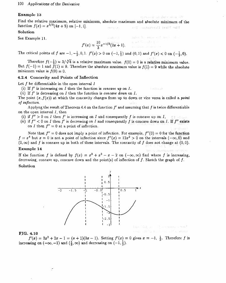
100 Applications of the Derivative
Example 13
Find the relative maximum, lrelative minimum, absolute maximum and absolute minimum of the function f(x) = x2f3(4z +!5) on [-I, 11.
Solution
See Example 1 1.
f1(x) = %-1/3(22 + 1). 3
The critical points of f are -1, -$, 0 , l . f t (z) > 0 on (-1,;) and (0 , l ) and f t(x) < 0 on (-4,0). Therefore f (-$) = 3 / ~ is a relative maximum value. f(0) = 0 is a relative minimum value.
But f (-1) = 1 and f (1) = 9. Therefore the absolute maximum value is f (1) = 9 while the absolute minimum value is f (0) = 0.
4.2.4 Concavity a n d Points of Inflection
Let f be differentiable in the open interval I (i) If f ' is increasing on I then the function is concave up on I.
(ii) If f ' is decreasing on I then the function is concave down on I. The point (x, f(x)) at which the concavity changes from up to down or vice versa is called a point of inflection.
Applyng the result of Theorem 4.4 on the function f' and assuming that f is twice differenbiable on the open interval I, then
(i) if f" > 0 on I then f t is increasing on I and consequently f is concave up on I , (ii) if f" < 0 on I then f ' is decreasing on I and consequently f is concave down on I. If f" exists
on I then f" = 0 at a point of inflection.
Note that f" = 0 does not imply a point of inflection. For example, f"(0) = 0 for the function f = x4 but x = 0 is not a point of inflection since f"(x) = 12x2 > 0 on the intervals (-oo,O) and (0, oo) and f is concave up in both of these intervals. The concavity of f does not change at (0,O).
Example 14
If the function f is defined by f (x) = x3 + x2 - x - 2 on (-00, m) find where f is increasing, decreasing, concave up, concave down and the point(s) of inflection of f . Sketch the graph of f .
Solut ion
FIG. 4.10 f'(z) = 3z2 + 22 - 1 = (x + 1)(3x - 1). Setting ft(x) = 0 gives z = -1, a. Therefore f is
increasing on (-00, -1) and ( 4 , ~ ) and decreasing on (-1, i ) .

f " ( x ) = 6x + 2 = 2(3x + 1). Therefore f " ( x ) = 0 at x = - 4. Thus f is concave down on (-00, - 4 ) and concave up on (-4,m) and x = -i gives a point
of inflection. The graph o f f is sketched in Figure 4.10.
Example 15
Let f ( x ) = x - sin x for x E (O,2n), find where f is increasing, decreasing, concave up and concave down and point(s) of inflection o f f .
Solution
f'(x) = 1 - cosx = 0 at x = 0, 2n. Therefore f' > 0 on (O,2n) and thus f is increasing on (O,27r). f " ( x ) = sinx = 0 at x = 0 , n , 2n, Therefore f"(x) > 0 on ( 0 , ~ ) and f"(z) < 0 on ( x ,2n ) . So f is concave up on (0, n), concave down on ( x , 27r) and has a point of inflection at ( n , n) .
0
4.2.5' The Second Derivative Test for Extremum
Another test for extremum besides the first derivative test is a test that depends on the sign of the second derivative at an interior criti&l point where the first derivative vanishes. From the discussion following the definition of concavity we expect that if a function has a critical point in an interval I and is concave up there (i.e. f" > 0 ) then it has a minimum on I. Similarly if a function has a critical point in an interval I and is concave down ( f" < 0 ) then it has a maximum there. More precisely we have the following result.
THEOREM 4.7 (SECOND DERIVATIVE TEST) Suppose f' and f" ezist in an open interval containing the number c and fl(c) = 0. Then
(a) fl'(c) > 0 * (c , f ( c ) ) is a relative minimum point. ( i i ) f"(c) < 0 a (c , f ( c ) ) is a relative mazimum point.
The nature of the critical point is not determined b y f"(c) = 0.
PROOF. Let us prove the result for f l(c) = 0 , f"(c) < 0 (i.e., part (ii)). By these hypotheses and definition of f"(c)
0 > fl'(c) = lim f t (c + h ) - flW = am f ' ( c + h ) h-0 h h-0 h .
Since lim f ' (c+ h, < 0 then by Theorem 2.1 of Section 2.2 there exists an interval 0 < Ihl < 6 h-0 h
within which f ' (c + h, < 0. For h > 0 , f1(c + h ) < 0 while for h < 0, f1(c + h ) > 0. Thus by the h
first derivative test f has a local maximum at (c , f ( c ) ) . The proof of part (i) is similar.
. - ,- 0 Example 16
Find the critical points of the function f ( x ) = 4x3 + 9x2 - 12% + 7 and test them for local extrema.
Solution f ( x ) = 4xs + 9x2 - 12x + 7
f 1 ( x ) = 12x2 + 18x - 12 = 6(2x2 + 3x - 2) = 6(2x - 1)(x + 2).

102 Applications of the Derivative
The critical points satisfy the equati,on
and hence x = -2 and 3 are the critical points.
1 15 Hence (-2, f (-2)) = (-2.35) is a local maximum while (i, f (i)) = (f, T ) is a local minimum.
Example 17
Find and classify the critical points of f (x) = x - 2 cos x in the interval ( -T , T ) .
Solution
The critical points of f (x) = x - 2 coax satisfy the equation f'(z) = 1 + 2ainx = 0. That is 1 sinx = - 5 which implies x = -?, - 5 .
f"(x)=2cmx f"(-$) =-&KO and fn(-i) = & > O .
Gs For x = -7, f(x) = 4- and for x = -%, f(x) = -&- t . Therefore (-?,a- v) is a local maximum while (-p, -fi - 5 ) is a relative minimum. Note that the end points are not included in the interval.
0
Exercises 4.2
For the functions in problems 1-4 find the intervals where each is monotone increasing, monotone decreasing, concave up, concave down and any point(s) of inflection.
1 f (x )=x3-6x2+12x-8 ' (x+2)(1-x) 2 f(x) = x
For the functions in problems 5-11 find the intervals where each is monotone increasing, mono- tone decreasing, concave up, concave down and any point(s) of inflection. Find also the critical points and uae the first or second derivative test to determine the relative extrema.

4.3 Applications of Maxima and Minima 103
11 f ( s ) = s 4 - 8 x 3 + l 0 x a + 4 0 12 f ( x ) = (z - 3)2'5(3x + 5 )
Determine all the relative maxima, relative minima, the absolute maximum and the absolute minimum of each of the functions defined in problems 13-17.
15 f ( x ) = 4x3 + 9za - 12. + 13, -3 < x < 2 16 f ( x ) = -2s' + x2 + 22 + 4, -2 5 x 5 2 3
4.3 Applications of Maxima and Minima
In the examples and problems that we discussed under maxima and minima in Section 4.2 we had often explicitly given the function to be extremized and our task had been to determine the critical points and test them for extrema. In this section part of the problem involves identifying the quantities to be exttemized, expressing them as functions of one variable by eliminating any other variables and then carrying out the extremization. Let us consider several examples.
Example 18
Prove that of all rectangles of given perimeter the one with the largest area is a square.
Solution
Let the perimeter of the rectangle be P and the length and width be x and y respectively. Therefore
The area, A say, of the rectangle is x y , i.e.,
A = x y .
The problem is to maximize the area A. We must first of all eliminate one of the variables, either x or y. From y = $ P - x we have
To extremize A we set A1(x) = 0 which implies
Now A"(+) = -2 <-0 and hence the critical point x = P/4 is a relative maximum. For
That is x = y and hence the maximum area is given by the square.
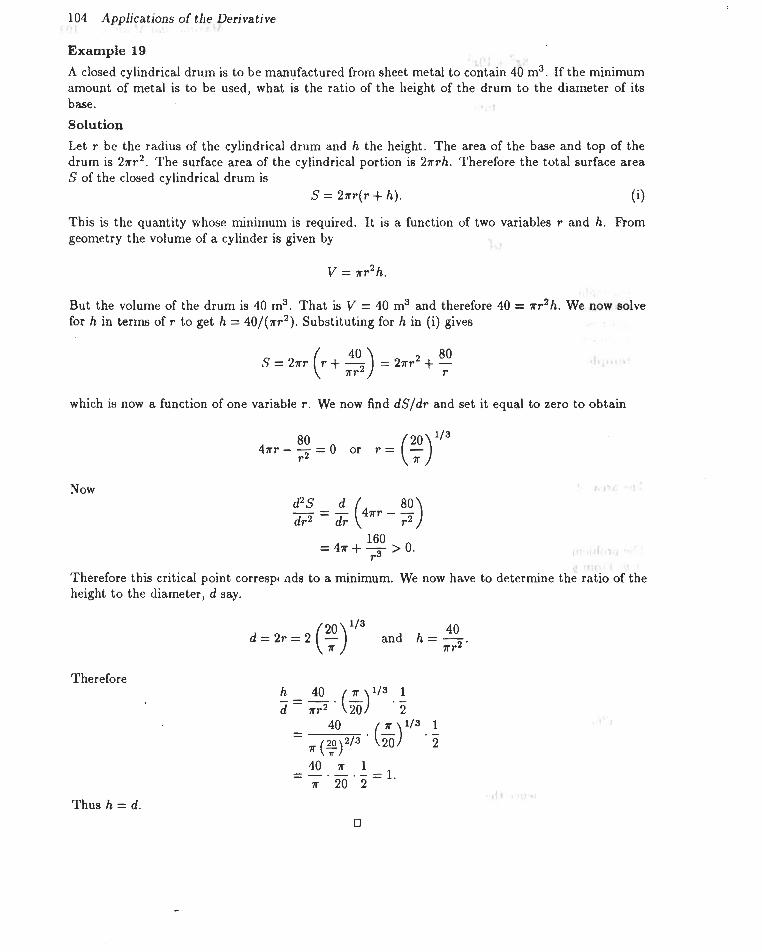
104 Applications of the Derivative
Example 19
A closed cylindrical drum is to be manufactured from sheet metal to contain 40 m3. If the minimum amount of metal is to be used, what is the ratio of the height of the drum to the diameter of its base.
Solution
Let r be the radius of the cylindrical drum and h the height. The area of the base and top of the drum is 2nr2. The surface area of the cylindrical portion is 2nrh. Therefore the total surface area S of the closed cylindrical drum is
S = 27rr(r + h) . (i)
This is the quantity whose minimum is required. I t is a function of two variables r and h. From geometry the volume of a cylinder is given by
But the volume of the drum is 40 m3. That is V = 40 m3 and therefore 40 = d h . We now solve for h in terms of r to get h = 40/(7rr2). Substituting for h in (i) gives
which is now a function of one variable r . We now find dS/dr and set it equal t o zero to obtain
Now
Therefore this critical point correspc nds to a minimum. We now have to determine the ratio of the height t o the diameter, d say.
Therefore
Thus h = d.

4.3 Applications of Maxima and Minima 105
Example 20
Consider a line given by Ax + By + C = 0, A and B not both zero. Find an expression for the distance between a fixed point (xo , yo) and any point ( 2 , y ) on the line. Minimize this distance to obtain a formula for the distance from a point (xo, yo) to a line Az + By + C = 0.
Solution
The distance d from (xo, yo) to ( x , y) on the line is given by
To ensure that the point ( x , y ) is on the line we must have
1 y = --(Ax + C ) for B # 0.
B
We shall consider the case B = 0 at the end. Therefore
2
( A x + + YO) d2 = (z - + 7 I t is more convenient to minimize d2 rather than d.
or x =
1 A2 + B2
( B ~ x ~ - AByO - AC)
and
The second derivative
A 1 C Y = - z ' A ~ + B ~ ( B ~ X O - AByO - AC) - - B
- - 1 A2 + 8 2
(-ABxo + AZyo - BC).
and therefore the critical point is a minimum. This minimum distance satisfies the equation
' 1 1 2
d 2 = [ A2 + 8 2
( B ~ X O - AByO - AC) - X O ] ~ + I A 2 + B2 ( -ABXO + A'YO - BC) - Y O ]

106 Applications,of the Derivative
Therefore
For B = 0 the line Ax + B y + C = 0 becomes the vertical line x = -CIA, (A # 0) and its distance l A X o + . This is a special case of (i) and hence (i) is valid for all lines.
0 Example 21
In microeconomics the pn'ce elasticity of demand, e, is defined as the negative of the percentage in quantity of goods demanded divided by the percentage change in price. Obtain an expression for the instantaneous price elasticity of demand. Suppose the demand for a product is given by X = a - bp where p is unit price, a and b are positive constants, find the maximum total expenditure on the product and the price elasticity of demand at this critical price.
Solution From the definition
Therefore d X P the instantaneous price elasticity of demand = -- - d p x
A ., Let TE represent the total expenditure. Then
Therefore
a d 2 T E The critical point is p = - and since - = -2b < 0 it corresponds to a maximum.
2b dp2
.. ,
The corresponding price elasticity of demand ie
a Example 22 . The product of two positive numbers is 36. What is the minimum value of their sum?
Solution
Let the numbers be x and y. Then xy = 36. The sum, S say, of the numbers is S = z + y. We wish to minimize S. To do so we eliminate one of the variables, y say. Thus

4.3 Applications of Maxima and Minima 107
d S 36 d 2 S 72 - = I - . - and - = - dx x2 dx2 z3 '
The critical points satisfy = 0. That is x = f 6. Of these values I = 6 is positive for which
- 2 > 0 and hence it gives a minimum. Since xy = 36 it follows that y = 6. Hence the minimum w - value of the sum is 12.
0
Example 23
Assume that the increase in consumption of an article is proportional to the decrease in the tax on it. If the consumption is c gm when there is no tax, and cl gm when the tax is n kobo per gm., find the amount of tax most profitable t o the ministry of finance which collects all tax revenues.
Solution
Let Y be the total tax accruing to the Ministry when tax is x kobo per gramme and z gm. is consumed. Then
Y = X Z . ( 4
We want this to bc the most profitable, that is the maximum collectable tax. Y is a function of two variables and we must eliminate one of them.
Since the increase in consumption is proportional to the decrease in tax it follows that the decrease in consumption c - z is proportional to the increase in tax x, that is
and assuming that k is the proportionality constant then
For c = c l , x = n, that is c - cl = kn, therefore
C - Z x -- - - c - c 1 n
from which it follows that
Substituting for x in (i) gives n(c - Z) y = - Z.
C - C 1
We now extremize Y with respect to z .
dY -- n -- d2Y 2n - -- ( c - 2%) and - - < 0. d~ c - cl d z 2 c - c1
The critical point is z = $ which is a local maximum. The most profitable tax t o the Ministry is

108 Applications of the Derivative
Exercises 4.3
The sum of two positive numbers is S. Find the maximum value of their product.
Find the shortest distance from the origin to the curve xy = 3.
Suppose one of the sides of any box that can be carried onto an airplane must be less than 8 in. find the maximum volume of such a box if the sum of the three sides (length, width and height) cannot exceed 46 in.
a Suppose that the demand X for a product is given by X = - + b - cp where p is the price per
n r unit and a , b and c are constants. Find the maximum income from sale of the product. Consider the x-axis as a mirror. Suppose a ray of light from a point source a t (x l , yl), yl > 0 arrives at a point (x2, y2), y2 > 0 after reflection from the mirror. Assuming that the time taken for the light to arrive at (xz, y2) is minimized (Fermat's priniciple), derive that the angle of incidence is equal to the angle of reflection. Prove that of all isosceles triangles with given perimeter the equilateral triangle encloses the largest area. An open water tank of square base is t o be made from a square sheet of metal of side 2 m. by cutting out square pieces from each of the four corners, lifting the resulting flaps and soldering the edges together (see sketch). Find the maximum capacity of such a tank.
1 Find the shortest distance from the point (10,9) to the curve y = -x2.
2 Suppose the cost of making x decorative clay pots is 150 + 502 naira and the potter can sell x pots per month a t 245 - 3.6252 naira on the road-side and 250 - 42 naira in the market. Find the most profitable number of pots the potter should make per month if she sells
(i) all the pots on the road side (ii) all the pots in the market
(iii) half on the roadside and half in the market. What is the total profit per month in each of the cases above?
A closed cylindrical tank of volume V m2 is to be constructed from two sizes of guage metal. The metal for the top and base cost twice as much per square metre as that of the cylindrical portion. What is the ratio of the height to the radius of the tank if the cost of construction is to be minimized. Consider the x-axis as the boundary between two media one occupying y > 0 and the other y < 0. Let the speed of light in the media be cl and c2 respectively. Suppose a ray of light from a point source a t (XI, yl), yl > 0 arrives a t a point (x2, y2), y2 < 0 after refraction through the boundary y = 0. Assuming that the time taken for light t o arrive a t (22, y2) is minimized (Fermat's principle) derive Snell's law i.e. if O1 is the angle of incidence and O2 is the angle of refraction then
sine1 sin O2 -- - -. c1 c2

4.4 Curve Sketching
Many of the properties of a function which we studied in the previous chapters and in the earlier sections of this chapter are useful in the sketching of the the graphs of such functions. Some of these properties are domains of definition, continuity, monotonicity, concavity, points of inflection and relative extrema. In this section we shall discuss a few other properties-intercepts, symmetry and asymptotes-and then apply these properties in sketching graphs of several functions.
The points at which the graph of a function y = f(x) intersects the axes are found by setting x = 0 and y = 0. The y-intercept, that is the intercept on the y-axis is easy to obtain, being f(0). The x-intercepts are also called the zeros of the function and they satisfy the equation f (x) = 0. If the function is defined implicitly the x- and y- intercepts are still obtained by setting y = 0 and x = 0 respectively.
Example 24
Find the x- and y-intercepts of the graphs of the functions (i) y = f (2) = 2x2 - 5x + 2 and (ii) x a c w y - y = 4 .
Solution
(i) To get the y-intercept, set x = 0 which gives y = 2. For the x-intercept, set y = 0 to get 2x2 - 52 + 2 = 0. That is (2x - 1)(x - 2) = 0 or x = $ or 2. Thus the intercepts are (0,211 (;lo) and (2,O).
(ii) Set x = 0 to get y = -4. For the x-intercept we set y = 0 to get x2 = 4 or z = f 2. Therefore the intercepts are (0, -4)) (-2,O) and (2,O).
4.4.1 Symmetry
Our everyday understanding of symmetry is that a figure is symmetric about a line if to every point of the figure on one side of the line there is a corresponding equidistant point (image) on the other side. Let us use this understanding to define symmetry about the coordinate axes. Consider first the y-axis. The image of a point ( t o , yo) with xo > 0 about the y-axis is the point (-xo, yo). See Figure 4.11. Thus a curve is symmetric about the y-axis if both the points (x, y) and (-x, y) satisfy the equation of the curve for all x. That is if the equation of the graph is unchanged when x is replaced by -x.
Similarly, a curve is symmetric about the x-axis if its equation is unchanged when y is replaced by -y. Observe that the graph of a function cannot be symmetric about the x-axis. (Why? How many values does it have for a given value of x?)
A curve is symmetric about the origin if its equation is unchanged when both x and y are replaced by -x and -y respectively so that both (x, y) and (-x, -y) lie on the curve.
FIG. 4.11

1 10 Applications of the Derivative
Example 25
Determine the symmetric properties of the graphs of each of the following functions
(i) y = 1x1-x2+3 (ii) 4x2 + gg2 = 36
(iii) xy = 3 u 3u (iv) s i n y = c a r x , - T < x < T , - ? < y < ~
Solution
(i) In y = 1x1 - x2 + 3 replacing x by -x given y = I - X I - (-xl2 + 3 = 1x1 - x2 + 3 and hence the graph of y = f(x) = 1x1 - x2 + 3 is symmetric about the y-axis. The relation changes if y is replaced by -y and hence the graph is not symmetric about the x-axis.
(ii) The relation 4x2 + 9y2 = 36 is the same if x is replaced by -x or y is replaced by -y or both x and y are replaced by -x and -y respectively. Therefore the graph of 4x2 + 9y2 = 36 is symmetric about the y-axis, symmetric about x-axis and symmetric about the origin.
(iii) Replacing x and y in xy = 3 by -x and -y respectively gives (-x)(-y) = 3 or xy = 3 and hence the graph is symmetric about the origin.
(iv) Replacing x by -r in sin y = cos x gives sin y = cos(-x) = cos x and hence the graph of sin y = cos x is symmetric about the y-axis.
The graphs of these relations are shown in Figure 4.12.
xy = 3 (iii)
FIG. 4.12
4x2 + 9x2 = 36 ( ii)

If the points on the graph of a function get closer and closer to the graph of a straight line as the points become more and more distant from the origin the straight line is called an asymptote to the graph of the function. Thus if P ( x o , f ( x o ) ) is a point on the graph of a function f then the graph of a line A x + By + C = 0 is an asymptote to the graph of f if
since / A x o + B f ( x o ) + C I / d m f is the distance from the to the line A x + By + C = 0 (See Equation (i) of Example 20 of Section 4 .3 ) is the distance of
coordinate axes. P from the origin. Let us consider special cases of ( 1 ) corresponding to asymtotes parallel to the
Asymptotes parallel to the x-axis
For the special case when the asymptote is a line parallel to the x-axis, such as y = b ( A = 0, B = 1,C = -b) Equation ( 1 ) may be shown to be equivalent to
iim If (xO) - bl = 0 Izol-00
which for x > 0 or x < 0 implies
( 2 ) lim f ( x ) = b or lim f ( x ) = b. 2-00 2--00
Example 26 x - 1
Show that the line y = 1 is an asymptote to the graph of f ( x ) = -. x
Solut ion
and r - 1 1
lim - - - lim 1 - - = 1 t - -w x I--00 x
FIG. 4.13
it follows that the line y = 1 is an asymptote to the graph of f both as x - ca and as x + -m. The graph o f f is shown in Figure 4 .13 .
Y
J T - - - - - - - - - - - + - - - - - - - - - - - -
- 4 -2 - 1
- 2
- 3
- 4
a x 2

112 Applications of the Derivative
Asymptote parallel t o the y-axis
For the special case when the asymptote is a line parallel to the y-axis, such as x = a ( A = 1, B = 0,C = -a) Equation (1) may be shown to be equivalent to
'That is either
2 - 1 Show that t11~ lir~c x = -1 is an asymptote to the graph of y = -. (2 + 1)
m d hcwcc 3' = I is a vcrtical asymptote.
0
'l'lic lil~lits in (3) ]nay he shown to he equivalent to either
(4 ) lim 1f(x)1=ca or lim If(x)l=ca. I-a+ x-a-
We shall use either of the forms (3) or (4) depending on which is more convenient.
Oblique asymptotes
For an oblique asymptote both Ixol and (f(x0)J become unbounded as the distance.from the point (to, f(xq)) to the origin becomes unbounded. It is therefore sufficient t o take 1x01 -) oo; that is, either xo -, ca or xn -) -MI in ( 1 ) . Thus the line Ax + By + C = 0 is an asymptote if either
Example 28 1
Show that the line y = x is an asymptote t o the graph of y = x + - X
Solution
For the line = x, A = -1 .B = 1 , C = 0 and IAxo+Byn+CI = I -xo+xo+&I = 1J-1 and JZTP = JZ. Now

4.4 Curve Sketching 113
1 Hence y = x is an asymptote to the graph of y = x+ -. The graph of the function and its asymptote
X is shown in Figure 4.14.
FIG. 4.14
In all the examples discussed above we gave the asymptote and then proceeded to prove the claim. It can be shown that a simple technique for guessing asymptotes is to drop the terms in the relations between the variable x and y that are negligible for large values of x or y or both. If the expurgated relation is a straight line then such a line may then be tested to determine if it is an asymptote. Let us reconsider the functions in Examples 26-28.
2 - 1 1 1 (i) For y = - = 1 - - we may neglect - for large x compared to 1. This gives y = 1 which
x x x was proved as an asymptote.
2 - 1 (ii) For y = - , we have x = - + and we may neglect 1 compared to y in both the numerator
x f l 1 - u " Y and the denominator to obtain that x approaches -- = -1 as y becomes unbounded. Hence v
x = - 1 is an asymptote. 1 0
(iii) For y = 1 x + l l we neglect - compared to x for large values of x to obtain y = x which is an
x - - asymptote.
xz As a final example we consider the relation -2- - - Y' - 1 = 0. Here for large values of x and y
a b2 ,. ,. 2'
we may neglect 1 to obtain - = - " which gives the pair of straight lines a2 b2
We leave the proof that these straight lines are asymptotes to the hyperbola as exercise. Let us now consider proper rational function y = % (a ratio of polynomials with no comrr~on
' zv factors). As x approaches any zero of q(x) the ratio y = becomes unbounded. Thus as y 4 oo
or y -, -oo x may be shown to approach any of the zeros of q and hence the lines x = xi where xi are the zeros of q(x) are vertical asymptotes to the graphs of the proper rational function y = %. This result also follows from the fact that as x approaches any of the zeros of q(x) the rational
function becomes unboynded and therefore by the relations (4) lim - = cm. 2-2, q ( x )
Example 29 I p(x) I
x 2 - 3 x + 2 Find the vertical and horizontal asymptotes of the graph of the function y = f (x) =
-. 2 2 - 31: .

1 14 Applications of the Derivative
S o h t ion
For horizontal asymptotes we observe that
lim x2 - 3 2 + 2 = lim
x2 - 3 x + 2 t.-m 2 2 - 3 2
= 1 22 - 3 2
and hence y = 1 is an asymptote. For vertical asymptote we note that
is a proper rational function and the denominator has zeros at x = 0 and x = 3 and hence the lines x = 0 and x = 3 are vertical asymptotes.
4.4.3 Curve Sketching
We have now discussed a large number of properties of functions that we need to enable us make detailed and accurate sketches of functions. Let us apply many of these in sketching the graphs of a few functions.
Example 30
x2 - 2x + 1 Analyse and sketch the graph of the function f defined by y = f(x) =
2 x 2 - 5 x + 2 ' Solution
Intercc.pts: For x = 0, y = $ and for y = 0, ( x - 1)2 = 0 =j x = 1. Asymptotes: Since lirn,,, y = 3 the line y = 3 is a horizontal asymptote. Setting ihc denominator = 0 gives (22: - l)(x - 2) = 0 or x = 4, 2. Therefore the lines x = 3 and x = 2 are vertical asymptotes. Critical points:
Therefore t itical-points are x = -1 and x = 1. The sign of y' is shown in the line sketc :h below.
Thus (-1,:) is a relative minimum while (1,O) is a relative maximum. The function f is monotone increasing on the intervale (-1,;) and (1,2) and monotone decreasing on the intervals (-w, -I), (391) and (2,001. Symmetry: There is no axis of symmetry.

2 . -* 3.
4.4 Curve Sketching l i 5
The graph of f is sketched in Figure 4.15.
FIG. 4.15
0
Example 31
Analyse and sketch the graph of the function f defined by y = f ( x ) = ( x - 3)2 /6 (3x + 5 ) .
Solution
Intercepts: For 2 = 0 , y = 5(9)'15; and for y = 0 , x = -:, 3 . Therefore the intercepts are ( 0 , 5(9)' / ' ) , (- !, 0 ) and (3,O) Asymptotes: The graph has no asymptotes. Criiical points: 2
y' = - ( x - 3) -3 /5 (3x + 5 ) + 3 ( x - 3)2 /5 5
Therefore the critical points are x = 3 and x = i. - ( 9 , l O E ) is a relative maximum while (3 ,O) is a relative minimum.
. -
Monotoniciiy: The function f is monotone increasing on ( -oo , i) and ( 3 , oo) and monotone decreas- ing on ( $ , 3 ) . Symmetry: There is no axis of symmetry. The graph of f is sketched in Figure 4.16.
FIG. 4.16

116 Applications of the Derivative
Example 32
Analyse and sketch the graph of the fundtion f defined by y = f(x) = (x2 - 1)(4x2 - 9).
Solution
I l l f e ~ c c p t ~ : X = 0 p = 9. Also y = 0 d (2' - 1)(4x2 - 9) = 0 Z = f l , f q . Asymptotes: The graph has no asymptotes. Symmetry: Replacing x by -x does not change the function and hence the graph is symmetric about the y-axis. Criltcal poznls: y' = 2x(4x2 -9)+8x(x2- 1) = 2x(8z2- 13). The critical points o f f are 0, f m. From the sign of f ' we conclude that f is monotone decreasing on (-co, - m), (0, m) and monotone increasing on (- m, 0) and ( m, 00).
y" = 48x2 - 26 = 48(x - d m ) ( x + d v ) and noting the sign of y'' we conclude that the graph o f f is concave up on (-00, - d m ) and (d13/24,m) and concave down on ( - d m , d m ) . Since y"(0) = -26 < 0 and y"(f m) = 52 > 0 it follows that (0,9) is a relative maximum while (f m, -25116) are relative minima. The graph o f f is sketched in Figure 4.17.
FIG. 4.17 0
Exercises 4.4
In problems 1-14 analyse and sketch the graph of each of the functions obtaining where applicable the intercepts, asymptotes, critical points, extrema and intervals where the function is monotone, concave up or concave down.
I X ' , consider x > 0 and x < 0. 10 y = - x - 1

4.5 Approximations of Functions 117
13 y=- I x - ' I , consider x > 1 and x < 1 2 1 14 y = x + T . x x
In problems 15-20 analyse and sketch the graph of each of the relations obtaining where applicable the intercept;, asymptotes, critical points, extrema and intervals where the graph is concave up or concave down.
15 y2 = x(z - 2)2 16 y2 = x2 - 1
4.5 Approximations of Functions
Suppose we wish to approximate a continuous function f in the neighbourhood of a point of continu- ity, a say, one immediate possibility is to approximate the value of the function in this neighbourhood by its value at the point. Geometrically this approximation corresponds to a horizontal line, namely y = f (a ) . On further consideration we may ask if the function is differentiable at a . If so then the graph of f has a tangent a t (a , f(a)) and we may then reasonably claim that the tangent to the curve a t the point would, make a better approximation than the value. That is, we expect that
would be a better approximation than y = j(a). This may be as far as our geometric intuition might lead us. Analytically we might observe that in the first approximation we matched the value of the function a t a . In the second, in addition to the value, we matched the slope (i.e. the first derivative) at a. Based on this we may then expect that the next step would be to also match the second derivative, then the third derivative and so on.
Let us proceed slowly. Before doing so we observe that there are some questions we need to answer as we proceed. One important question is: how good are the approximations? Another related question is how large are these neighbourhoods. We start by revisiting the Mean Value Theorem.
By the Mean Value Theorem if f is a function continuous on an interval [a, b], differentiable on (a , b) then there is a point c E (a, b) for which
Replacing b by x in the above result gives
(5) f(x) = f(a) + fl(c)(x - a) for some c E (a, x).
Thus if we wish to approximate f(x) by f(a) the error e(x) 1 f(x) - f (a)l is given by
e(x) = If(.) - f(a)l = I fl(c)l 1x - a1 for some c E (a,x)
5 Ix - a ] maxIflI.
That is

118 Applications of the Derivative
where the maximum is taken over the interval ( a , x ) . The same result is valid for x < a except that the maximum is taken over ( x , a ) . The result (i) gives us the maximum value of the error as the product of the size of the neighbourhood and t,he maximum value of the derivative of f' in the neighbourhood.
We may then write
f ( X I f (a )
with an error e < 1x - a1 . max I f ' l . Example 33
Find the maximum error made in approximating f ( x ) = x2 - 4 x + 1 by its value a t x = 1 in the interval Ix - 11 5 i. For what interval is the maximum error less than lo%?
Solut ion
f ( 1 ) = -2, f' = 2 x - 4. The interval is Ix - 11 < f which implies % 5 z 5 a. Now
on this interval. Therefore 1 5 5
error < - . - - - 4 2 - 8 '
Suppose thedesired intervalis lz-11 < 6, thensince lx-21 = lx-1-11 _< 13:-lI+I-11 5 Ix-lI+1
Therefore maximum error = 26(6 + 1) . The percentage maximum error is
1 1 That is.6(6 + 1) = - Solving for 6 gives 6 = -(m - 1) and the desired interval is lx - 11 c
10' 2
Let us now consider the next higher order approximation, called the linear approximation.
Result
Suppose f and f' are continuous on [a, b] and f" exists on ( a , b) then there exists a point c in ( a , b) such that
PROOF. Let us suppose that there is a number A such that
f ( h ) = f (a) + f1(a)(b - a ) + A(b - a)2.
We wish to determine A. Define a function F by
F ( x ) = f ( x ) - f ( a ) - f l ( a ) ( x - a) - A ( z - a)'.
( ii)
(iii) '04

4.5 Approximations of Functions 119
By ( i i ) F (b ) = 0. But F ( a ) = 0. Since F satisfies the hypotheses of Rolle's Theorem there is a point cl in ( a , b ) such that F1(c1) = 0. From (iii)
F 1 ( x ) = f l ( x ) - f l ( a ) - 2 A ( x - a) .
Now F' satisfies the conditions of Rolle's Theorem on [a, c l ] since P is continuous on [a, q], dif- '.
ferentiable on ( a , c l ) ! F 1 ( a ) = 0 and F1(cl) = 0. Therefore there is a point c E ( a , c l ) such that Ft'(c) = 0. Thus 0 = F1'(c) = f " ( c ) - 2 A or
which is the desired result.
0
Replacing b by x in (i) gives
(6) 1
f ( x ) = f ( o ) + f l ( a ) ( z - a ) + p f " ( c ) ( x - a)'
for some c 6 ( a , x ) . Thus if we wish to approximate f (x) by the tangent f ( a ) + f l ( a ) ( z - a ) the error e ( x ) is given by
1 5 :(x - a)2 max ( f l ' l .
We may then write
with an error 1
e 5 -12 - a12. max I f " l . 2
This is called the linear approximation.
Example 34
Find the maximum error made in approximating f (z) = x2 - 4x + 1 by the tangent a t x = 1 in the interval ) x - 11 5 i.
,'. ; * Solution
f = x 2 - 4 x + 1 , f' = 22 - 4 and fl' = 2. The approximating function is
f ( 1 ) + f l ( l ) ( x - 1 ) = -2 + ( -2 ) (x - 1) = -22
and the error e ( x ) is 1
e ( x ) = f n ( l ) l ( x - I ) ? = ( x -

120 Applications of the Derivative
Therefore maximum error in Ix - 11 < is $. The graph of f and the approximating functions of Example 33 and the tangent are shown in' Figure 4.18.
FIG. 4.18
'I'll(- results (5) and (6) may be generalized to give the following.
'I'IIEOREM 4.8 (TAYLOR'S THEOREM) Suppose f , f', . . . , f(") are continuous on [a, b] and f("+') exzsts on (a ,x ) then there is a point c E ( a , x) such that
I':quat,ion (8) is called Taylor's Formula or Taylor's Approximation. The proof of this result is beyond the scope of this text. The special case of n = 2 is given as
a n exercise. A concliision we may draw from the above is that we may improve the approximation to a function if we include more terms in (8) and reduce the size of the neighbourhood of the point n about. which the approximation is made.
From (8) we may write the approximation
The error e(x) satisfies
1 e(x) 5 -1x - aln . max I f ( n + l ) l ,
(n + I)!
For a = 0 we write below the cubic approximation (i.e. terms up to x3) for a number of functions.

4.5 Approximations of Functions 121
Example 35 '
Derive the first four terms of the Taylor's approximation for f ( x ) = f i given above.
Solution f = ( 1 - x)1/2, f l = - + ( I - x)-1 /2 , f* = - : ( I - .)-312 and f1I1 = - ! ( I - z)-'f2,
Therefore 1 1 f ( 2 ) iJ f ( 0 ) + f l ( 0 ) . + % f I 1 ( O ) x2 + 3f111(0)x3
Differentials
Let y = f be a function of the independent variable x . A small change, A x , in this independent variable at a point x = a is called the difleren2ial o h and is also denoted by d x . For such a change in x , the corresponding change in the dependent variable A y is given by
Based on the linear approximation (7), where x - a = A X ,
we have A y ss f l ( a ) A x = f l ( a ) d z .
The combination f l ( a ) d x is called the differential of the dependent variable y a t x = a and is denoted by d y . Thus while the differential dx of an independent variable x is the change in the independent variable A x , the differential d y of a dependent variable y , is the linear approximation of A y a t the point. That is
A y % d y f l ( a ) d x .
Let us use the differential to compute some approximations.
Example 36
Use differentials to find the percentage error made in computing the area of a square-shaped farm if the tape used in measuring its sides has stretched by 0.1%. Is the area overestimated or underes- timated. Find the exact percentage error.
Solution Let x be the lenith of each side of the farm. Then the area, A, of the farm is
dx A A Since - = 0.1% then - = 0.m.
x A

122 Applications of the Derivative
The area is overestimated since the measuring tape gives a value larger than the actual value fcit eqch length measured.
cet us compute the exact error.
Therefore
dx dz Now - E 0.1% which implies that - = 0.001 and hence
x x
Th~rcfore the error is 0.2001%.
Exercises 4.5
Determine the linear approximation to each of the functions in Problem 1-4 at the given point xo and find the niaximunl error in the given interval.
X X X f(x) = sinx. x" = g. Ir - <
Derive the quadratic approximation a t 3 = 0 for each of the functions in problems 5-8.
Derive the cubic approximation at x = 0 for each of the functions in
f (2) = sin x 10 f ( x ) = z c o s x
problems 9-12

4.6 Indeterminate Forms and l'H6pital's Rule 123
13 This problem concerns the proof of Taylor's Theorem for n = 2. Let f , f' and f" be continuous on [a, b] and f"' differentiable QII ( a , b). ,We wish to prove that there is a point c 6 (a ,b ) such that
1 1 f ( 6 ) = f ( a ) -t f ' ( a ) ( b - a ) + - f " ( a ) (b - a12 + - f l"(c) (b - a)3
2! 3!
1 Let F ( x ) = f ( x ) - f ( a ) - f l ( a ) ( x - a ) - - f " ( a ) ( x - a ) 2 - B ( x - a)3.
2 a. Assume that F(b) = 0. Use Rolle's Theorem to show that there is a point cl in ( a , 6)
such that F 1 ( c l ) = 0. b. Show that F' satisfies the conditions of Rolle's Theorem on [a, c l ] and deduce that there
is a point c2 in ( a , c l ) such that F1'(c2) = 0. c. Show that F" satisfies the conditions of Rolle's T h e ~ r e m on [a, c2] ant1 deduce that there
is a point c in ( a , c2) such that FU'(c) = 0 and hence deduce (9).
4.6 Indeterminate Forms and l'H6pital's Rule
Let us consider the determination of limits of functions that are expressible as quotients of two functions where both the limit of the numerator and that of the denominator are zero. That is, suppose a function f is defined by
with lirn g ( x ) = 0 and lim h ( x ) = 0. z 4 e x-C
We seek 9 ( ~ ) lim f ( x ) = lim -
I-c x-c h ( x ) '
The rule for the limit of a quotient (see Theorem 2 . 6 ~ of Section 2.3) does not apply since lim h ( x ) T; x-c
0. Such a limit which would ordinarily lead to 8 is called an indelerminate form. Recall that the application of the definition of the derivative in determining the derivative of
a function alwa$s leads to a g indeterminate form since
We have aheady discussed how to handle such indeterminate forms when the functions g and h are polynomials (see the remark following Example 13 of Subsection 2.3.1). In such cases we first reduce the rational function t o its proper form, %. In this form, if limr-, p(x) = 0 then lim,,, f ( x ) = 0, while if lirn,,, q ( x ) = 0 then lim,,, 1 f ( x )1 = m.
Let us now consider how to determine limz+, f ( x ) = lirn,-, when the functions g and h satisfy some differentiability conditions at c.
THEOREM 4.9 (L'H~PITAL'S RULE) Suppose two functions g and h are such that g(c) = 0, h(c ) = 0 and gl(c) and hl(c) exist with h l (c ) # 0 then

124 Applications of the Derivative
PROOF. Since g and h are differentiable a t c, they are both continuous there. Consider the ratio
R ( x ) = 9 ( 4 - 9(c) . - c x # c.
x - c h ( x ) - h(c ) '
Also
Therefore g ( x ) - gl(c) provided hl(c) # 0. lim - - -
x-c h ( x ) hl jc)
For some quotients of functions both g' and h' may vanish a t c. For such functions the following stronger version of 17H6pital's rule which we state without proof may be used.
Result (1'HBpital's Rule)
Suppose the functions g and h are differentiable in an open interval containing the number c and
lim g ( x ) = 0 and lirn h ( x ) = 0 r - C 2 - C
then g ( x ) g l ( x ) provided hl(c) # 0. lirn - = lirn -
2 - c h ( x ) I - c hl(+)
0 Remark 4.1
(i) If both gl(c) = 0 and hl (c ) = 0 then I'H6pital's rule may be applied again provided g" and hI1 exist in some interval containing c to give
9(x> g l ( x ) lim - = lim - = lim L@ provided h1I(c) # 0. c h ) r - c hl(+) z-c hl'(x)
This may be repeated as many times as necessary until either g(")(c) or h(")(c) is nonzero.
(ii) If the other conditions of Theorem 4.9 are met but hl(c) = 0 while gl(c) # 0 then
(iii) Note that it is not the quotient f which is differentiated but the numerator and denominator are differentiated separutely.
Example 37
x 2 - 2 - 2 Find lirn
1-1 1 - x2
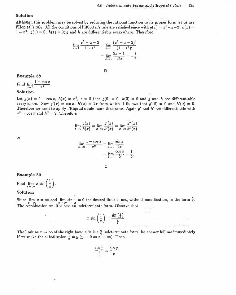
4.6 Indeterminate Forms and l'H6pital's Rule 125
Solution Although this problem may be solved by reducing the rational function to its proper form let us use 1'Hbpital's rule. All the conditions of l'H6pital's rule are satisfied since with g(x ) = x2-2-2, h ( x ) = 1 - x2; g ( l ) = 0, h(1) = 0; g and h are differentiable everywhere. Therefore
x 2 - 2 - 2 ( x 2 - 2 - 2)' lim = lim 2 - 1 1-22 1 - 1 ( l - x 2 ) l
2 x - 1 1 - lim - - -- - 2-1 -22 - 2'
Example 38 1-cosx
Find lim 2-0 x2
Solution Let g ( z ) = 1 - cosx, h ( x ) = x2 , c = 0 then g(0) = 0 , h(0) = 0 and g and h are diffcrentiable everywhere. Now gl (x) = sinx, h l (x ) = 22 from which it follows that g'(0) = 0 and hl(J) = 0. Therefore we need to apply 1'Hopital's rule more than once. Again g' and h' are differentiable with g" = cos x and h" = 2. Therefore
1 - cosx sin 2 lim = lim - 2-0 x2 2 4 0 22
cosx 1 = lim - = -. 0 4 0 2 2
Example 39
Find lim x sin (:). 1-00
Solution 1
Since lim x = oo and lim sin - = 0 the desired limit is not, without modification, in the form E. 1+03 0+00 x
The combination oo -0 is also an indeterminate form. Observe that
sin (i) x sin (:) = T. -
2
The limit as x -, oo of the right hand side is a 8 indeterminate form. Its answer follows immediately if we make the substitution = y ( y -+ 0 as x -+ oo). Then
sin 1 sin y 0=-
1 - 2 Y

126 Applications of the Derivative
which has the limit 1 as y 4 oo. Let us however retqin the variable x and use l'H8pital's rule.
Example 40
1 1 Find lim (- - -) .
2-0 xainx x t a n x Solution
Recall that as x -t 0, sin x -+ 0 and tan x -t 0 and both x sin x and z tan x are positive in some neighbourhood of x = 0. Therefore
1 1 lim - r cm and lim - = oo. 2'0 x sin z t4O x tanx
The desired limit is therefore of the form oo - oo. This is another indeterminate form. In this case, as in many such cases, it may be reduced tr, a indeterminate form.
1 1 1 cosx 1-cosx - = - = ; . , xsinx z t a n x xsinx z s inx x s m z
Therefore 1-cosx
sin x = lini by l'H6pital's rule z - ~ s i n x + xcosz
cos x = lim by l'H6pital's rule t-o 2cosx - xsinx
- - 1 - 5'
We have discussed how to obtain limits of indeterminate forms of the form $, 0-oo and oo-oo. There are other indeterminate forms such as 2, l w , Ow and ooO. The last three of these shall be considered in Chapter 7. Let us conclude this section by mentioning another form of l'H6pital's rule.
Resul t
Suppose lim,,, g ( x ) F cp and lim,,, h(z) = oo then
if the latter limit exists.

4.6 Irtdetcrminate Forms and 11H6pital's Rule 127
The proof of this result. is beyond the scope of this t,ext,. Let us use it to revisit some of the limits we had donc by alternate ~netliods.
3e2 - 4 x + 7 Find lim
r--oo 2 --I - S r 2 '
Solution From the above result
Exercises 4.6
Find the indicated limits. sin n x
lim - r-1 r - I
sec x - 1 lirn r-o 1 2
2x2 + x lirn
x--4 2x2 - x - 1
1 - cos n x lirn t--0 sin n x
82 lim(x - 1) tan - r+ 1 2
lim 1 - J C - 2
r-+O 1-cosx
x 2 - 4 x lirn -
r - m 3 - 5x2
lirn (: - cse x) r, x-0
tan z 4 lim --
x-0 2
sin" lim x-O 1 - cos 2
]in1 z tan (:) z-c.3
3 - 4 ~ : + 2~~ lirn
r-m 7 - L.a + 5 2 3
sin 2x 14 lirn -
r-n x - 7
sin x tan x lim (F - -) x- 0 33

128 Applicatio~ls of the Derivative
Miscellaneous Exercises
1 Find the equation of a line that is tangent to the curve y = x 2 + 22 + 1 and is perpendicular to the line 32 + 4y = 2.
2 Find the slope of the tangent to the graph of the given equation a t the given point. (i) = 3 - x 3 , ( - 4 ( i i ) /1z2 + y2 = 5 , ( 1 , - 1 ) .
In problems 3-5 firid the critical points and relative extrema of the given function and also where it is monotone, concave up and concave down.
Analyse and sketch the graph of f defined by f ( x ) = x - - I 4 4 - x2
Analyse and sketch the graph of f defined by f ( x ) = - 2 - 1
Find the quadratic approximation to f ( x ) = 2x3 - 4x + 7 at the point x = 1. What is the r~iaxin~urn error of the approximation in the interval lx - 11 < $?
Find the quadratic approximation to f ( x ) = ,/%& a t x = 0.
sin x x lim r-2 2 2 - 2 - 2 11 lim
dl + 3s" 2-00 x + 4

The Integral
I n Chapter 4 we discussed how to find a function which is the derivative of a given function. Here we shall first consider the inverse process, called antidifferentiation, that is, given the derivative of a function to find the function. Then we shall discuss integration which enables us to solve the problem of finding the areas of plane regions. The two processes of antidifferentiation and integration are related by the Fundamental Theorem of Calculus which we prove.
5.1 The Antiderivative
Let us recall some problems of derivatives solved in the earlier chapters. There we determined that the function f(x) = x had the (derivative ft(z) = 1) constant function 1 as its dcrivativc. A sketch of the function and its derivative is shown in Figure 5.1.
a. Graphof f ( w ) = x h. Gr~ipIi ~ t ' d ~ r i v a ~ i v ~ of 1: I~;,II,+ ,,.) = 1
FIG. 5.1 Note that for any real number C the function f(x) = x + C also has the const,ant function 1 as its derivative. Sketches of the function f (x) = x + C and its derivatives for various values of C are shown in Figure 5.2.
Graph of .r+C for C ' = X . { .o.-l b. Graph of thc tlcrius~ivc r~ in~t lon
FIG. 5.2 Similarly the function f(x) = 4x - x3 has the derivative 4 - 3x2 and functions of the type
4x - x3 + C where C is a constant also have the same derivative 4 - 3z2. Figure 5.3 shows the -

130 The lntegrai
*ketches of these functions for some values of C and the derivative. 1%
1'
-6.
--8-
FIG. 8.3 Now we consider the reverse problem of determining functions for which a given function is
the derivative. For example, from discussions above, we note that the function F ( z ) = r + C for C constant are the desired functions for which f ( x ) = 1 is the derivative and the functions F ( x ) = 4x - x3 + C are the ones for which f ( x ) = 4 - 32' is the derivative. Such functions are called antiderivatives. More precisely we have the following definition.
DEF~NITION Let f be a real valued function defined on a set S. A function F defined on S such that
D F = F ' = f
on S is called an antiderivative o f f on S.
In view of the discussion preceding the above definition we have that the functions x + C are antiderivatives of the function 1 on R and the functions 4x - x3 + C are antiderivatives of the function 4 - 3x2 on R. Example 1
Since cos x is the derivative of sin z therefore sin x is an antiderivative of cos z on R. The functions sin x + C are also antiderivatives of cos x on R.
Based on the above one may ask the question: Are all antiderivatives of f where F' = f expressible in the form F + C where C is constant function? The following example helps in answering the question.
Example 2 1
Find the antiderivatives of - x= '
Solution 1 1 1 1
so -- is an antiderivative of >. Also -- + C where C is a constant x x x
1
is antiderivative of A Besides these 2 2 '

5.1 The Antiderivative 131
1 1 is also an antiderivative of - Thus F(x) is not of the form -- + C for some real number C!
x2 ' X
Thus in general the answer to the question above is No. But by (MVT Chapter 4) we have the fol lo~ing result.
THEOREM 5.1 Let the junctions F and Fl be antiderivatives o j ihe junction f on an interval (a, b). Then
Fl = F + C
where C is a constant junction on (a, b ) .
PROOF. By definition Fi = / and F' = j. Therefore
By Theorem 4.5 FI - F is a constant function, C. Therefore
With the understanding that we shall consider only functions defined on open intervals, we introduce the notation D" to represent antiderivatives. Thus for f defined on (d, b) and F' = f on (a, b)
where C , usually an arbitmy constant stands for the set of all constant functions on ( a , b). In general, the expression (1) shall be written even for functions f whose understood domain
is not necessarily an open interval, with the understanding that the equation is valid for all open intervals (a, b) contained in the understood domain.
Thus, we may write
taking it to he valid over the open intervals (-m,0) and (0,oo) separately.
1 Show that x4 + 3x is an antiderivative of 4x3 + 3. Find the antiderivative of 4x3 + 3 which has the value 0 at x = 1.
2 Find the value of a if ax2 + 1 is an antiderivative of x.
3 Find the valueof b if bxn+' is an antiderivative of xn.
4 Show that 1x1 is an antiderivative of sgn (2) on the open intervals (-m,0) and ( 0 , ~ ) . Is D-'sgn (x) = 1x1 on R.

132 The Integral
5.2 Antiderivatives of Some Elementary Functions
Our ability to determine antiderivatives depends to a large extent on our knowledge of the results about derivatives. Let us review some of these results here.
Recall that (see Sections 3.3-3.5)
Dxn = nzn"
Ds inx = cosx
D cos x = - sin x
D t a n x = s e c 2 x
n c o t x = - C S C ~ X
Dsecx = secxtanx
D csc x = - csc x cot x.
Also, in general, for differentiable function F and G and a constant k
for u a differentiable function of x. From these we get the following antiderivative formulas.
1 D- lXm= xm+l + C , m f - 1 m + l
D-'cosx = s i n x + C .
D-'sinx = - C O S X + C D-' sec2 x = tan x + C
D - ' C S C ~ X = - c o t x + C
D-'(sec x tan x) = sec x + C
D-'(cscxcotx) = - C S C X + C D-'(f k g ) = D-'f f ~ - ' g
D-'(k f ) = kD-'f
D-'(DJD,~) = ~ ( u ) + c .
Note that in (19) and (20) we have not included an arbitrary constant function C. This is because the. antiderivatives have not actually been determined on the right hand side of each of those equations.
Observe that (12) can be verified by using (2) and (10) as follows. For m # 1

5.2 An tiderivatives of Some Elementary f inc tions 133
So by Theorem 5.1 ,
Example 3
Find (i) D - ' ( x ' / ~ ) (ii) 0 - ' ( x 2 + s i n x ) (iii) D- ' ( s inx-cosx+4) .
Solution
(ii) By (19) 0 - ' ( x 2 + sin x) = 0 - ' x 2 + 0-' sin x 1 =, -x" cos x + C by (12) and (14). 3
(iii) D-'(sin x - cos x + 4) = D-'(sin x - cos x) + 0 - ' 4 by (19) = ~ " a i n z - ~ - ' c o s x + ~ - ' 4 by (19)
- - - cos x - s inx + 42 + C by (14), (13) and (12).
In seeking the antiderivative of a function we express the given function as a sum of functions whose antiderivatives we know or as a product of a constant and a function whose antiderivative we know.
Example 4
Find (i) D-l(x(x + I ) ) (ii) D-' ( y) ,
Solution
(ii)
= D-l (x + $) = D-l x + ~ D - ' X - ~ by (19) and (20)
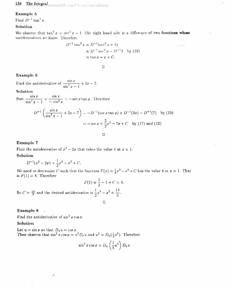
184 The Integral
Example 5
Find D- ' tan2 E .
Solut ion
Wc observe t.liat tar,' x = sw:! 3' - 1 . ' 1 ' 1 ~ right. ]land side is a difference of two function8 wh& ar~tiderivativcs wc know. 'l.'hercforc
I)-' tan' x = ~91)-'(sc!c% - 1)
= I)-' sec2 z - I > - ' 1 by (19) = t a n x - x + C .
Example 6 sin 2
Find the antiderivative of +3.r - 7. sin' x - 1
Solution sin z - sin x
Now - - = - sec z t.an s. 'I'11erc:fore s i n 2 x - 1 -COS%
D - I ( sin x = - D-' (sec E tan x) + 0-I (32) - U - ' ( 7 ) by (19)
sin2 x - 1 3 = - s e c z + Tx' - 7x + C' by (17) and (12) . 2
Example 7
Find the antiderivative of x2 - 21: that. takes the value 4 a t x = 1.
Solut ion 1
D-'(x' - 2 2 ' ) = -x3 - x2+C:. 3
We need to determine C' such that the function F ( z ) = 5x3 - x2 + C l ~ a s the valuc 4 at z = 1. That is F(1) = 4. Therefore
1 F(1) = - - 1 + c = 4.
3 1 9 14
So C = and the desired antiderivative is -s3 - xu + --, 3 3
Example 8 ,
Find the antiderivative of sin2 x ccos x.
Solut ion
Let u = sinx so that D,u = cosx. Then observe that sin2 2:cosx = u2D,u and u2 = UU, (4u3) . Therefore
sin2 r cos x = D, ( i u 3 ) D=U

which is of the form (1 1) with f ( u ) = gu3. Consequently by (2 1 )
Therefore
Example 9
Find the antiderivative of x(x2 + 3)4 .
Solution
Let u = x2 + 3 then D,u = 2x. Now observe that
and
Thus x(x2 + 3)4 = D ~ ( $ U ~ ) D , U which is of the form ( 1 1 ) with f(u) = hu5. Therefore by (21)
Example 10
Find D-' (Jxl ) .
Solution
In order to use ( 1 ) let us first find an antiderivative of 1x1 vaIid on R. For x > 0 , It1 = I therefore
1 D-'(lxl) = D-'X = -x2 + K1
2 where I\'' is a constant function. For x < 0 , 1x1 = *-I therefore
where K 2 is a constant function. Based on the above we consider the continuous function G defined by
+ x 2 2 2 0 C(E) =
-;x2 X < 0 .
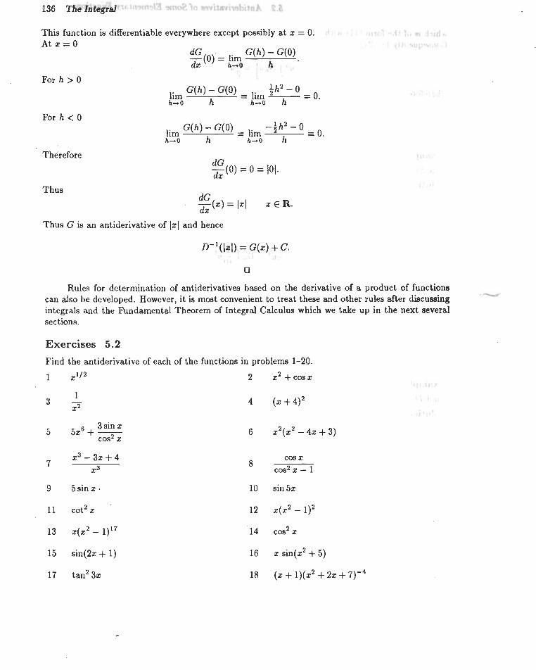
136 The Integral
This function is differentiable everywhere except possibly a t x = 0.
For h > 0
For h < 0
Therefore
Thus
Thus G is an antiderivative of 1:) and hence
Rules for determination of antiderivatives based on the derivative of a product of functions . - can also be developed. However, it is most convenient to treat these and other rules after discussing integrals and the Fundamental Theorem of Integral Calculus which we take up in the next several sections.
Exercises 5.2
Find the antiderivative of each of the functions in problems 1-20.
x1/2
1 - x2
3 sin x 5x6 + -
cOs2 x
x3 - 3x + 4 x3
5sin x
cot2 x
X ( X ~ - 1)17
sin(2x + 1)
tan2 32
x2 + cos 2
Cos x cos2x - 1
sin 52
x(x2 - 1)2
cos2 x
x sin(x2 + 5)
(x + 1)(x2 + 22 + 7)-4
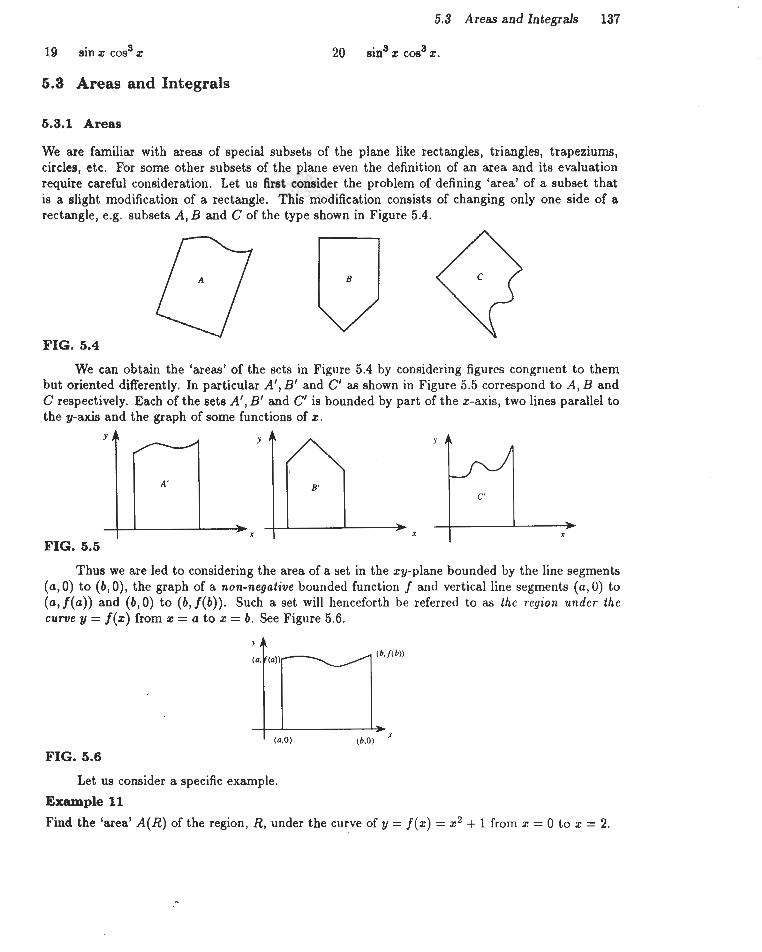
5.3 Areas and Integrals 137
3 19 sin x cos x
5.3 Areas and Integrals
5.3.1 Areas
We are familiar with areas of special subsets of the plane like rectangles, triangles, trapeziums, circles, etc. For some other subsets of the plane even the definition of an area and its evaluation require careful consideration. Let us first consider the problem of defining 'area' of a subset that is a slight modification of a rectangle. This modification consists of changing only one side of a rectangle, e.g. subsets A, B and C of the type shown in Figure 5.4.
FIG. 5.4
We can obtain the 'areas' of the sets in Figure 5.4 by considering figures congruent to them but oriented differently. In particular A', B' and C' as shown in Figure 5.5 correspond to A, B and C respectively. Each of the sets A', B' and C is bounded by part of the x-axis, two lines parallel to the y-axis and the graph of some functions of z.
FIG. 5.5 I
Thus we are led to considering the area of a set in the xy-plane bounded by the line segments (a, 0) to (b, O), the graph of a non-negative bounded function f and vertical line segments (a, 0) to (a, f(a)) and (b,O) t o (b, f(b)). Such a set will henceforth be referred to as the region under the curve y = f(z) from x = a t o x = b. See Figure 5.6.
FIG. 5.6
Let us consider a specific example.
Example 11
Find the 'area' A(R) of the region, R, under the curve of y = f (x) = x2 + 1 from x = 0 to x = 2.

Solution
The region is shown in Figure 5.7 ' y A
FIG. 5.7 d A
We note that the region R is contained in the rectangle OACD and contains the rectangle OA B E. Therefore
Let us partition the interval OA into two equal subintervals OA1 and AIA as shown in Fig. 5.8
FIG. 5.8
Now the area of the region R is greater than or equal to the sum of the two rectangles with base OA1 height f(0) and base AIA and height f(1). See Fig. 5.9a. A(R) is less than or equal to the sum of the areas of the two rectangles with base OA1, height f (1) and base AIA height f (2). (see Fig. 5.9b) Thus
( ii)

5.3 Areas and Integrafs 139
FIG. 5.9
If we partition the interval OA into three equal subintervals OA1, A I A and A2A then the area of the region R is greater than or equal to the sum of the areas of the shaded rectangles in Fig. 5.10a and less than or equal to the sum of the areas of the three shaded rectangles in Fig. 5.10b.
FIG. 5.10 a. b.
Thus 2 2 ,f(O) + ;, (3) + f f (4) 5 4 . 1 5 if (f) + 3f ($) + f f (2 )
(iii)
Observe that as the number of partitions increases the left hand side of the inequalities increases (2 ,3 ,8 , . . .) while the right hand side decreases ( 1 0 , 7 , 9 , . . .). In each case A(R) still lies between these numbers. This suggests that as the number of subdivisions increases the left hand side and right hand side of the inequalities get closer and closer to A(R). If it so happens that the left hand side and the right hand side tend to the same number, A* say, as the number of subdivisions increases indefinitely then A* should be A(R), the area of the region.

140 The Integral
Let us check if this is the case for the region under consideration. We take n subdivisions where n is any positive integer. For such subdivisions the areas of the rectangles t o be summed are shown in Figure 5.11.
y
d24 2 *
I I I I I I n n n n n b.
FIG. 5.11 Thus
.- - since Y 1 = 'V 1 = n
since 1' + 22 + 32 + . . . + m2 = m(m + 1)(2m + 1) 6
Therefore
!(I-;) 3 ( 2 - : ) + 2 < A ( ~ ) < ! ( l + ; ) 3 (2+:)+2.
Now
and 4 14 lim [: ( I + + ) ( 2 + 3 +2] = j . 1 * 2 + 2 = - .
n-m 3
Thus in this case there is a unique number A* = 9 and so
A(R) = area of region = - 3 '
- . - 0

5.3 Areas and Integrals 141
The same behaviour as in the above example will be exhibited by any non-negative continuous monotone function on a closed interval. [a, b].
The above analysis indicates the importance in the context of are? of sum of areas of rectangles erected below and above the graph of a non-negative bounded function. Other technical consider- ations motivate the introduction of a more general notion of an 'integral' of a bounded function f , using slightly modified sums. We discuss this below.
5.3.2 The Integral
A finite set P = {to , X I , . . . , xn) of points in [a, b] such that
i s called a partation of the interval. Given a partition, P = {xo, X I , . . . , x,) say, if we introduce one or more points the resulting partition, Q say, is called a finer partition than P .
Recall that a subset S of real numbers R is called bounded if there exist numbers 1 and u such that
s c [I, ul
i.e.. for all x E S,l 5 x 5 u. Every non-empty bounded subset of R has a least upper bound (or sup) and a greatest lower bound (or inf).
A function f : [a, b] +R is said to be bounded if there exist real numbers m and M such that
m 5 f(x) 5 M for all x in [a,b]
Given such a bounded function f and a partition P = {xo, X I , . . . , x n ) of the interval [a, b] we have real numbers
mi =inf{f(x) : x i < x 5 Xi+l)
Mi = SUP{~(X) : xi 5 x 5 xi+l)
for each i , i = 0 , 1 , . . . , n - 1. Thus we may form the sums
Those sums are respectively called the lower sum and upper sum for f corresponding to the partition P. These quantities are signed sums of areas of certain rectangles as indicated in Figure 5. 12.
4
a. FIG. 5.12

It can be shown that, if P = xo, X I , . . . , x, and Q = xb, x i , . . . , XL are partitions of the interval [a , b] where Q is finer than PI then
m(b - a ) I U f I P ) < L(fl'Q) and U(f ,Q) 5 U ( f , P ) I M(b - a).
'I'hese inequalities say t,hat a3 the partitions is made finer the lower sum tends t o increase while the upper s u m t m d s to decrca..~. Every lower sum is smaller than every upper sum.
Then wc can define real numbers
~ ' ( f ) = s u p { ~ ( f , I-') : P a partition of [a, b]) and Ua( f ) = inf(L(f, P ) : P a partition of [arb])
which have the property m(b - a) < La(f) < U'(f) 5 M(b - a).
DEFINITION A bounded function f : [a, b] -.R is said to be integrable (Riemann integrable) if and only 2f
L*y.) = U * ( f )
and for such functions this number L*(f) or U*(f) is called the definite integral o f f and is denoted bv
In short 0
[ f ( z ) d x = L*( f ) = W ( f ) and m(b - a ) < f ( x ) d x 5 M(b - a). Lb It can be shown that a bounded function f is integrable if and only if given any E > 0 there is a partition P of [a, b] such that
Wfl P ) - L ( f , P ) I E .
In particular, if given E > 0 there exists a partition Pn of [a, b] in n equal subintervals such !hat
i.e. lim U ( j , P,) = lim ~ ( f , P,) n-+w nda,
then the function is integrable and
1' f ( l ) d l = lim U( f , P,) = lirn L( f , Pn) . n-ao n-w
THEOREM 5.2 Let f : [a, b] - + R be a monotone function, then f i s integrable.
PROOF. We shall prove the result for monotone increasing functions. Consider P, = (xO, ~ 1 , . . . , x,) where a = xo < 11 < 2 2 < . . . < a, = b and
b - a xi+1 - xi = - for i = O , l , . . . , n - 1.
n

5.3 Areas and Integrals 143
Then
and
- b - a -- n [ f (21) + f (22) + ' ' . + f (xn)] .
Thus
lim U( f , Pn) = lirn L( f , Pn) n d w n-w
which establishes the desired result. The reader should prove the theorem for monotone decreasing functions.
In view of the above results, it follows that for any non-negative monotone function f defined on la, bl
[ f ( z ) dx is the area of the region under the graph of the function.
The result of the last theorem can be extended to functions f : [a, b] +R for which there are points a = to 5 t1 5 ... 5 tm = b , m E R+ such that for each subinterval [ t i , t i + l ] , i = 0,. . . , m - 1 , f is monotone. Such a function is referred to as piecewise monotone.
We note without proof the following result.
THEOREM 5 .3 Every continuous function f : [a, b] -+ R is integrable.
It follows from the above discussions that if f < 0 for all [a, b] then
-Lb f (x) dz is the area of the region above the graph of the function but below the z-axis.

144 The Integral
Example 12
If k is a positive constant function, then J: k dx is the area of the shaded rectangle in Figure 5.13.
FIG. 5.13 Therefore
0
Example 13
J: x dx for a , b > 0 is the area of the trapezium indicated in Figure 5.14.
FIG. 5.14
Therefore
Example 14
Find lb x3 dx, b > 0.
Solution
The integral exists since x3 is monotone increasing. Let us consider the partition P,, of equal
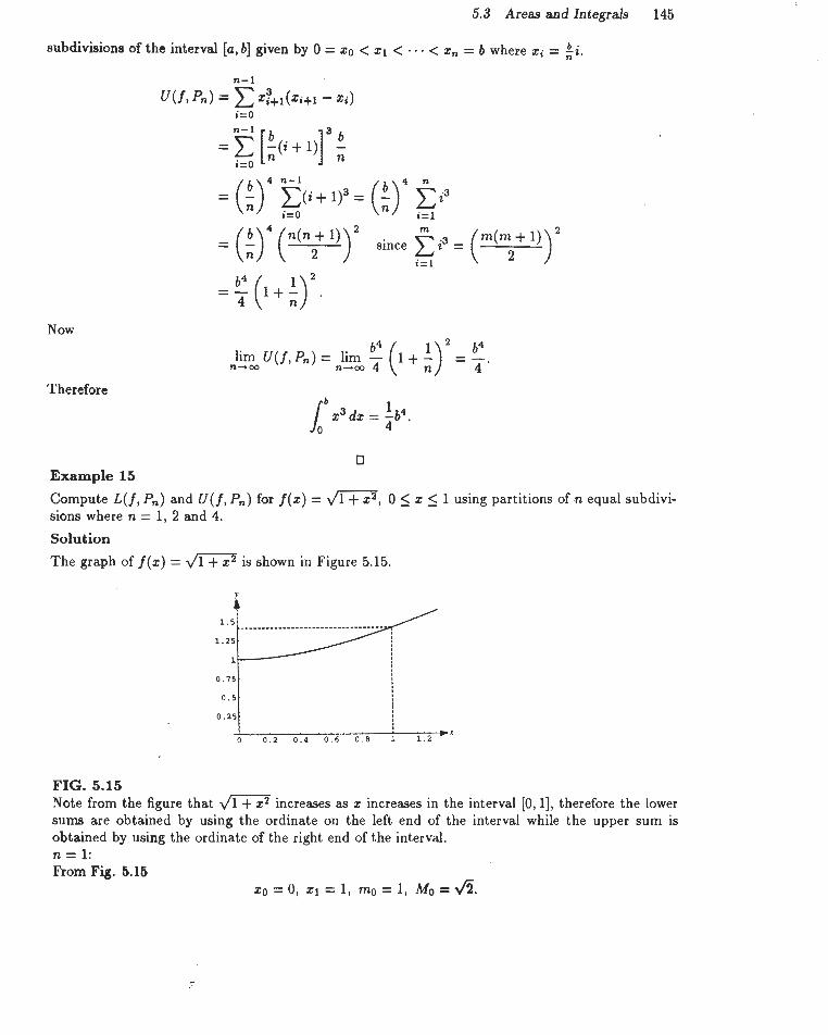
5.3 Areas and Integrals 145
b e subdivisions of the interval [a, b] given by 0 = so < XI < . . < zn = b where xi = --a.
Now
Therefore
0 Example 15
Compute L( f, Pn) and U( f, Pn) for f (x) = JEf, 0 5 z 5 1 using partitions of .n equal subdivi- sions where n = 1, 2 and 4.
Solution
The graph of f (x) = 4- is shown in Figure 5.15.
FIG. 5.15 Note from the figure that d w increases as z increases in the interval [ O , l ] , therefore the lower sums are obtained by using the ordinate on the left end of the interval while the upper sum is obtained by using the ordinate of the right end of the interval. n = 1: From Fig. 5.15
xo = 0 , X I = 1, mo = 1, MO =d.

146 The Integral
Therefore
4 5 MI = f (;) = -j-, M2 = f (f), = q, Ms = f(1) = JZ.
Therefore
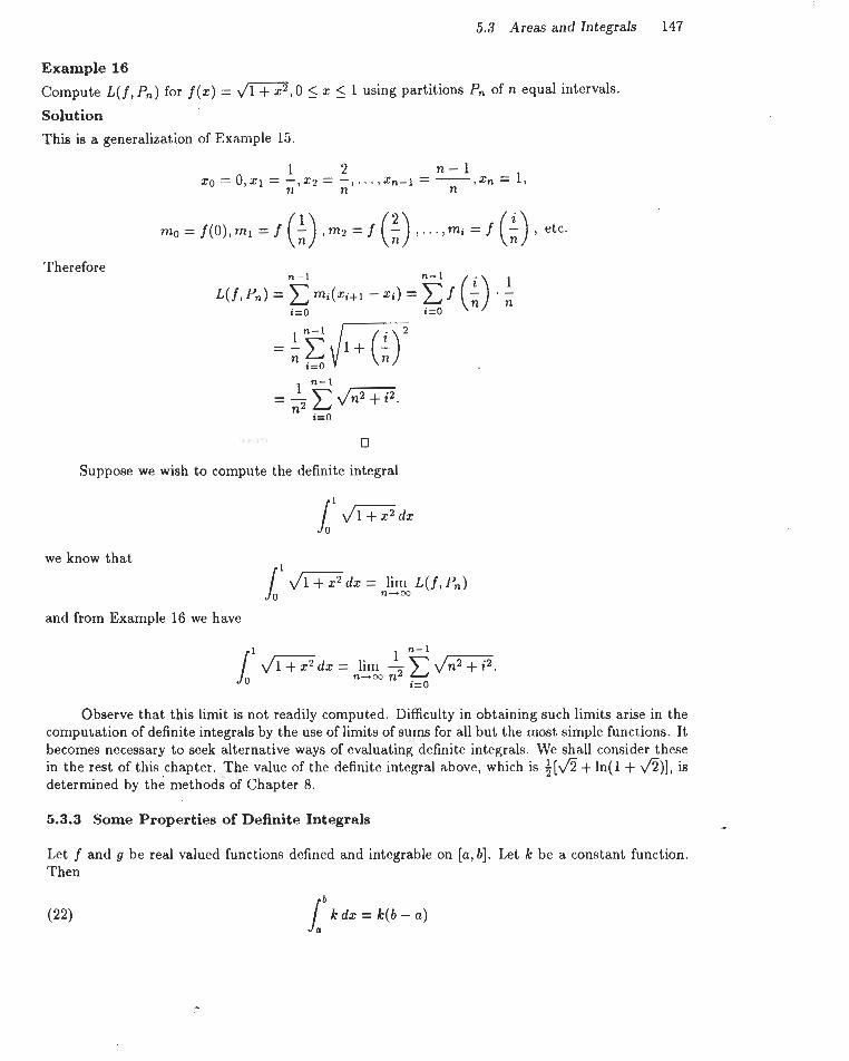
5.3 Areas and Integrals 147
Example 16
Compute L(f, P,) for f (z) = d m , 0 5 5 1 using partitions Pn of n equal intervals.
Solution
This is a generalization of Example 15.
rno=f(o),rn, =f(') ,m2=f (t) , . . , ,mi = f (A) , etc.
Therefore
Suppose we wish to compute the definite integral
we know that
and from Example 16 we have
1 * - I l 1 ~ - d x = n-m lim - c J ~ . n2
i = O
Observe that this limit is not readily computed. Difficulty in obtaining such limits arise in the compu~ation of definite integrals by the use of limits of sums for all but the most simple functions. It becomes necessary to seek alternative ways of evaluating definite integrals. We shall consider these in the rest of this chapter. The value of the definite integral above, which is 3 [fi + ln(1 + fi)] , is determined by the methods of Chapter 8.
5.3.3 Some Properties of Definite Integrals
Let f and g be real valued functions defined and integrable on [a, b ] . Let k be a constant function. Then

148 The Integrd
f + g and f - 4 are integrable and
for any point c in [a, b].
b
(26) 1 f ( x ) dx 5 1 g(x) dx if f (0 ) < g(x) for all 2 E [a, b]
If m 5 f ( x ) 5 M then for all x E [a,b] then
b
m(b - a) < 1 f ( x ) dx 5 M(b - a).
The proof of (22) is contained in Example 12. We shall prove (23) and leave the others as exercises.
PROOF OF (23 ) . Let P = { a = xo, 2 1 , . . . , xn = b) be a partition of the interval [a, b]. Let
then n-1 n- 1 1 k f ( x ) do = n-oo lim x mi ( ~ i + l - xi) = n-a, lim x k m r ( ~ i + l - x i ) i=O i=O
= k lim x rni(xiC1 - x i ) n-m
b
= k l f ( x ) d x .
Observe that the proof hinges on the fact that inf k f ( x ) = k inf f (2). . 4
DEFINITION Suppose f is integrable on [a, b] with b 2 a then
b la f ( x ) dx i s defined as - f ( 2 ) d ~ .

5.3 Areas and Integrals 149
If we take b = a in the above definition it follows that
la f (x) dx = 0.
Based on this definition we remove the restriction on c in (25). That is
for any numbers a, b and c provided all the integrals exist. For, suppose c > 6 > a , i.e, b E [a, c] then by (25)
lC (9 hut by definition
Therefore ( i ) implics b
1' f(z) dr = LC f (x) d z + 1 /(x) d*
which is the claim.
Example 17
Given that 1 ll f(x)dx = A . [ f(a)dx = 8 and l4 f (2) dx = C
1
(iii) f (x) dx.

150 The Integral
Example 18
Show that 1' d g d x 5 2. - 1
Solution
The function f (z ) = d-2 is defined and continuous for 1 - x2 > 0. Let us find the maximum value of f on [- 1, l ) .
and hence f attains its maximum 1 at x = 0 . Thus
Therefore by (27)
a Example 19
1 1 Show that 1 xsin5 r d r 5 -.
2 Solution
Since sin 3: < 1 for all z it follows that xsin5 z 5 x. Therefore
1 1 1 xsin5xdz <i xdx
but by Example 13 the second integral is
hence the desired result follows.
Exercises 5.3
In problems 1-4 compute L( f , P,) and U(f, P,) for each of the given functions on the given interval and for partitiohs of n equal subdivisions where n is given.
1 f ( x ) = x + l , 0 5 x 5 2 , n = 4 2 f ( x ) = x 2 , 0 5 x 5 3 , n = 3
Find the integrals in Problems 5-14 given that J!~ f (r) dz = A, J: f(x) dx = B , fl f (z) d t = C , J!2 g(x) dx = D, J: g(z) dx = E, 1. g(x) dx = F.

3
Show that 1 (x2 - 42 + 5) dc > 2.
1
Show that 1 eos3 x dx j 1.
x Show that - < x for z > 0 and hence that
x 2 + 5 - 5.4 Fundamental Theorem of Integral Calculus
.- - In Sections 5.1 and 5.2 we discussed the concept of the antiderivative. In the last section we used limits to compute areas of regions under graphs of functions and introduced the concept of the integral. In this section we shall discuss the fundamental theorem of integral calculus which relates the two concepts of antiderivative and integral and enables us to compute areas, volumes and other quantities that are definable in terms of definite integrals.
Suppose f is a function that is continuous on an interval [a, b] and hence integrable there. Then the quantity
defines another function of the variable x. See Figure 5.16. Denote this function by F(x).
FIG. 5.16 Let us determine
F(x + Ax) - F(x) DF(x) = lim
Ax-O AX

152 The Integral
Let us evaluate this limit when f is monotone increasing. Consider the case A x > 0.
which is the area of the cross-hatched strip in Figure 5.16a for the case f > 0. Since f is monotone increasing then for x 5 t 5 x + A x
f ( 2 ) 5 f ( t ) I f ( f + A x ) . Therefore by (27)
z+Az
f (.)Ax 5 f ( t ) dt 5 f ( x + A x ) A x .
Dividing by A x and taking the limit as A x + O+ gives
x+Az
lim f ( x ) 5 sz ('I d' 5 lim f ( X + AX). Az--O+ AX Az-O+
Since f is continuous lirn = f ( x )
Ax-O+
and hence by the Sandwich Theorem
lirn J,"+~" f ( t ) dt
Az-+O+ AX = f (2 ) .
Therefore F ( x + A x ) - F ( x )
lim = lim s,"+~" f ( t ) dt
Az-o+ AX Az-O+ AX = f(4.
Consider the case A x < 0.
which is the negative of the area of the cross-hatched region in Figure 5.16b for the case f > 0. Again since f is monotone increasing then for x + A x 5 1 5 x
Dividing by -Ax gives
(ii)
Since lirn f (3 ) = f ( x ) = lirn f ( x + AX
As-0- Az--0-
5.4 Fundamental Theorem of Integral Calculus 153
then by the Sandwich Theorem
F ( x + Ax) - F(x) lim = lim
- Jxx+Az f dt Az-0- AX Ax-0- AX = f (2).
We have thus proved a special case of the following very important and revealing theorem.
THEOREM 5.4 (THE FUNDAMENTAL THEOREM OF INTEGRAL CALCULUS) I f f is conlinuous on [a, b] then F(x) = Sr f (t) dt is diflerentiable on [a, b] and
A proof of Theorem 5.4 without the requirement of monotonicity fo1Iows the same scheme as that preceeding the statement of the theorem except that (i) or (ii) is replaced by
respectively and noting that since f is continuous
lim min f ( t ) = lim max f ( t ) = f ( ~ ) . Az-0 Az-0
Let us derive two corollaries of Theorem 5.4
Result
Every continuous function has an antiderivative.
PROOF. Let f be continuous on [a, b]. By Theorem 5.4 the function
is an antiderivative of f since D f = f .
THEOREM 5 .5 I f f is continuous on [a ,b] and F is any antiderivative o f f then
PROOF. By Theorem 5.4 the function
is an antiderivative of f . Thus both F and G are antiderivatives of f . By Corollary of Theorem 4.5 of Section 4.2, since G' = F' = f then
154 The Integral
where C is a constant. Therefore
which is the desired result. . - 0
We note that Theorem 5.5 is sometimes also called a Fundamental Theorem of Integral Cd- culus.
Example 20
Find 1 2 ( r + I ) d x .
Solution
An anliderivativc of x + 1 is F(x) = + x. Therefore by Theorem 5.5
Observe that by Theorem 5.5 any antiderivative would give the same reeult and so in evaluating definite integrals it is unnecessary to introduce the antiderivative constant which is also known as the constant of integration.
A convenient way of representing the right hand side of (i), namely F(b) - F(a), is
Thus for example
2=2
( i Z 2 + x) I means (iz' + +) - (5x2 + .) t=o evaluated at 2 = 2 evaluated at S=O
Based on the Fundamental Theorem of Integral Calculus relating antiderivatives and integra- tion another notation used in denoting antiderivative ia the integral sign without any limits appended to it. These are shown in two possible forms in Equations (30) and (31) below.

5.4 hndamental Theorem of In t e g d Calculus 155
D;'{ 1 z I{ }dx. Example 21
~ i n d & .in z dx . Solution
Rom (14) and (30) 1 ain z = - cos z. Therefore by Theorem 5.5
0
~xampie aa Find the area of the region bounded by the curve y = f (x) = 62 - x2 - 5 and the x-axis.
Solution
y = f ( z ) = 6 x - x a - 5 = ( 1 - x ) ( x - 5 ) .
Therefore the graph of the function intercepts the x-axis at x = 1 and x = 5. Also y > 0 in the interval [1,5]. Sec Figure 6.17.
FIG. 5.17 The desired area, A say, is
Now D-'(6x - z2 - 5) r 3x2 - Q x 3 - 52. Therefore by Theorem 5.5

156 The Integral
Exercises 5.4
5 Find 1 2 ( r 2 + x + 4) dz
7 Find L ( x 3 + Ix) dx
2
Evaluate 1 x5 dx
Find l r l 2 cos x dx
Evaluate [ y (32' + 1) dx
~ 1 3 Determine 1 secx tan xdx
In problems 9-12 find the area of the region bounded by the graph of the given function and the x-axis
9 y = f ( x ) = z Z - 2 x 2 10 y = x - 4
5.5 Integration by Substitution
In Section 5.1 we discussed how to find antiderivatives of functions by recognizing the derivatives of several classes of functions. One very important class of functions consists of functions which arise from the derivative of composite functions, that is, functions that may be expressed in the form
where u is a function of x . As observed there in Equation (21)
This last equation may be expressed in terms of the integral sign of (31) as
or in alternative notation as
Thus, td find the integral, S f dx, of a function f we seek to express f in the form
where the functions F and u are to be determined. The first step is to 'guess' u(x) from the form of f and thereafter determine F. Usually for each function f there is a fairly limited number of choices of u. Experience which comes from solving numerous problems of this type enables the reader to make an appropriate choice for u. Thereafter the determination of F may not be routine but it

5.5 Integration by Substitution - 157
should be easier than the determination of f without the introduction of u. This process is called method of substitution.
Examples 8 and 9 of Section 5.1 were solved by this method: Review them. Let us consider several more examples. .
Example 23
Find j' X I / - dx.
Solution
There are a number of choices for u. These include u = x , u = x2, u = 4 + x2 and u = d w . The first of these u = x accomplishes nothing since it leaves us with the original problem:
Thus if u = x then du = dx and
Here Fi(u) = u d w while f ( x ) = x d m which is the same function. The substitution u = x always leaves the integral unchanged and hence is never used.
The second of the choices u = x2 gives the following:
1 u = z 2 ~ d u = 2 ~ d x ~ x d x = - d u a n d 4 + x 2 = 4 + u .
- 2 Therefore
Here Fi(u) = ; ( 4 + ~ ) ' / ~ . To determine the last integral we may need to make another substitution, namely v = 4 + u.
The third of the choices u = 4 + x2 gives the following:
Therefore
Here Fi(u) = 3 ~ " ~ . Integrating to obtain F(u) gives
1 1 11 d l 2 dU = - + 6 ) = --usl2 + C where C = -C 2 2 2
Finally the fourth of the choices u = d w gives the following:
Therefore

168 Tbe Integral
Here Ft(u) = u2. Integrating to get F gives
1 - - - 3 ((AX)' +c) = f ( 4 + z')~/' + C where C = -C 3
We note that the last two substitutions give us Ft(u) whose integral we readily identified. Any of these substitutions is acceptable. In fact the second substitution is also adequate if we recognize that
or as we noted there.we may make a further substitution v = 4 + u. l l y it.
Remark 5.1 0
(i) In general there is no unique substitution.
(ii) In solving problems any substitution that lea+ to the determination of the integral is adequate.
(iii) Always remember to eliminate your substitution variable so as to express the indefinite integral in terms of the original variable.
(iv) It may sometimes be necessary to make two or more successive substitutions.
(v) The intermediate constants c in the above are really not necessary. What is important ie to add ail arbitrary constant function at the end of the integration process. In the next example we shall again consider more than one substitution for pedagogical reasons.
Thereafter only one substitution will be presented.
Example 24
Find 1 sin3 z cos z dz.
Solution
Two possible substitutions are u = sinz and u = cosx. Consider first u = sin z =$ 2 = cos z or du = cos z dz. Therefore
Now conbider u = cos z a 2 = - sin z or du = - sin z dz. Therefore
sin3 z cos x dz = sin2 x - cos x . sin z dz = (1 - cos2 z) COB z . sin z dz = (1 - u2)u - (-du)
Therefore

l a =--cos X + - C O S ~ X + C ~ . 2 4
(ii)
As the reader may show .by invoking the trigonometric identity sin2 x + cos2 x = 1 the two results (i) and (ii) are the same. Observe that C2 = Cl + 4.
n Example 25
Find S sin(5z - 2) dx.
Solution
Let u = 52 - 2 then du = 5 dz or dz = 4 du. Therefore
Suppose we wish to evaluate a definite integral f (x) dx for which the method of substitution is to be applied then we may proceed in one of two ways. One method is to first find the indefinite integral
by (32). Then it foIlows that rb
J. f (x) dx = F(u(b)) - F(u(a)).
Alternatively, when we make the sustitutiop u = u(x) we also change the limits of integration to u(a) and u(b) respectively to obtain.
. , Example 26
1 x + 3 217 Find 1' 2 ( y-) dx.
Solution

Therefore 7 x + 3
917 3 7
dx = - ?i (T) 1 = - (2g/7 - 49/7)
Example 27
Evaluate S;(X + 1)(x2 + 22 + 3)5 dx. Solution
Let u = x2 + 22 + 3 then du = (22 + 2) dx = 2(x + 1) dx. This implies that (x + 1) dx = 3 du. When x = 0, u = 3 and when x = 2, u = 11. Therefore
Example 28
Find S & dx. Solution
Let u = l n x then 2 = or d u = $. Therefore
2 dx = 2/ $ = 21n lul + C
Example 29
Evaluate
Solution
As the reader'may readily verify by carrying out the process the obvious substitutions u = 4-x2 and u = d n do not give a simpler integral than the original. An effective substitution is x = 2 sin a. For this dx = 2 cos u du and
Therefore dx J du = u + C.

5.5 Integration by Substitution ' 161
In the last example we used a substitution that may not appear obvious. We postpone further discussion of the method of substitution and other methods of integration to the last chapter.
Exercises 5.5
Find each of the integrals in problems 1-8.
6 1 cos5 x sin x dx
Evaluate each of the definite integrals in problems 9-12.
Miscellaneous Exercises
Find the antiderivative of each of the functions in problems 1-4.
3 sin x cosx
4
5 Use the definition of the integral to find 1 x2 dx
6 Show that
7 Show that if g is integrable then - :x 1'' g ( t ) dt = 2x9(x2) .
8 Evaluate J:, ( x 2 - 3 ) d x .

162 The Integral
9 Evaluate J$ cot r csc x dr .
10 Find the area of the region bounded by the graph of y = x 2 - x - 2 and Ihc x-axis.
11 Find the area of the region in the first quadrant bounded by the curves y = x2, y = 2 - x ant1 the x-axis.
12 Find J J m d z .
13 Find j' cos2 x sin3 x dx.

Applications of Integration In this chapter we shall use the concepts of antiderivative and integrals to compute areas, volumes and lengths of arcs. These quantities are definable by limiting processes that lead to definite integrals. Let us start with areas of plane regions defined in Section 5.4.
6.1 Areas of Plane Regions
Recdl that the area under the graph of a continuoue function f (x) betweeen x = a and x = b (a < 6) is J: f (z) dx for f (z) 2 0 on [a, b] while for f (z) < 0 on [a, b] the area is - I,' f (x) dz. In general the area of the region between the graph of y = f(z) and the z-axis in the interval [a, bJ is
Example 1
Find the area A of the region bounded by the curve of y = z3 - 3x2 - x + 3, the z-axis and the lines 5 z = O a n d x = 2 .
Solution
Since y = f(z)=z3-3z2-z+3= (x+l)(z-l)(e-3)) f(z)? Ofor -1 < z s 1 and x z 3and f (x) 5 0 for z 5 -1 and 1 5 z < 3. Therefore
5 f(z) 2 0 on [o, 1) and f(z) < 0 on [I,
See Figure 6.1. Hence
FIG. 6.1

164 Applications of Integration
An antiderivative of f ( x ) = x3 - 3x2 - x + 3 is F ( x ) = ax4 - x3 - i x 2 + 32. Therefore
We next consider a plane region bounded by x = a , x = b ( a < b) and the graphs of two continuous functions y = f ( x ) and y = g(x ) . Suppose that f ( x ) 2 g ( x ) for all a < x < b as shown in Fig. 6.2.
FIG. 6.2
Then the area A of PQRS is given by area of PQUV- area of SRUV. That is
b b
A = f ( x ) dx - JO 9 ( x ) dx ( 1 )
b =I" [ f ( 2 ) - g(x )] dx = 1 h ( x ) dx (see Fig. 6.2).
We call h ( x ) d x an element of area and the Riemann sum of such area elements gives the area. Observe that if g ( x ) = 0 in ( 1 ) A reduces to the area between the curve f ( x ) and the x-axis ( y = 0 ) in the interval a 5 x 5 b which is J: f ( x ) dx .
Example 2
Find the area A of the region bounded by the curves yl = 1 - x 2 , y2 = x + 2, and the lines x = 1 and x = 3.
Solution
Observe that ( x + 2) - ( 1 - x 2 ) = x2 + x + 1 > 0 for all x. Hence the curve y2 = x + 2 lies above

6.1 Areas of Plane Regions 165
yl = 1 - x2 for all x.
The area A = [(z + 2) - (1 - z2)] dz l3
Example 3
Find the area of the region bounded by the curves yl = z2 + 1, y2 = 4 - z2 and the lines z = f 1.
Solution
The two curves y, = x2 + 1 and y2 = 4 - x2 intersect where x2 + 1 = 4 - z2; that is, at x = f m. Therefore in the interval -1 5 ,x 5 1 the two graphs do not intersect and one is above the other. To determine which is above we evaluate these functions at any point z in (-1,l). Taking x = 0 we have 4 - x 2 = 4 > 1 = x2+ 1. Hence 4-x2 > z2 + l in -1 < x < 1. See Fig. 6.3.
FIG. 6.3
The required area A = [(4 - x2) - (x2 + I)] dx
0 Example 4
Find the area of the bounded region between the two curves y = x2 + 2 and y = 32. Solution
The curves intersect where z2 + 2 = 3x, that is z2 - 32 + 2 = (z - 2)(x - 1) = 0 which gives x = 1

166 ~pphcstions of Integration
or 2 (See Fig. 6.4).
FIG. 6.4
Required area = [3+ - (za + 2)] d x = (32 - za - 2) d~ I' I' = 1
1 6 '
0 Example 5
Find the area A of the region in the first quadrant bounded by the curve y r 2' + 1, the y-axis and the two lines y = 2, y = 10.
Solution
A sketch of the region is shown in Fig. 6.5.
Here the region is bounded by the y-axis, two lines parallel to the x-axis and a curve..In previous examplea we had a region bounded by the x-wis, two lines parallel to the y-axis and a curve. Hence the roles of x and y are interchanged. Thus, in particular, the.interva1 [a, b] over which the partitioning and subsequent integration are done is on the y-axis. The required area is therefore a

6.1 Areas of Plane Regions 167
sum of area elements of the type z dy (See Fig. 6.5). Hence
Use integration to find the area of a triangle.
Solution
Rotate the triangle so that a side lies on the y-axis with one corner at the origin (See Fig. 6.6).
FIG. 6.6
Let the ceordinates of A and B be (0, b) and (k, h) respectively. The equation for A B is
h - b yi=b+-x k
and that for OB is
Area of triangle = (yl - ya) dx Ik
1 = - (base length) x height. 2

168 Applications of Integration
Exercises 6.1
In problems 1-5 find the area of the region whose boundaries are given.
y = 3x2, the x-axis, x = 1, x = 4.
x3 y = -, x-axis, x = 0, x = 4.
3 y = x2 - 92, x-axis, x = 0, x = 3
x = 4,/5, y-axis, y = 4, y = 9.
x = 16 - y2, y-axis, y = -4, y = 4.
Find the area of one of the regions bounded by the curves y = sin x and y = cos x.
Find the area of the region between the x-axis and the curve y = sinx for 0 5 x 5 n. Find the area of the three regions bounded by the curve y = x(x - 1)(x - 2)(x - 3) and the x-axis. In problems 9-13 find the area of the region bounded by all the given curves.
x + 2 y = 2 , y - x = 1 , 2 x + y = 7 .
y = x2, y = 8 - x2, y = 4 x + 12.
y = x 2 , 2 x + y + 1 = 0 , x - 5 = 0 .
Find the area of the region bounded by the parabola y = 5 + 22 - x2 and the chord joining (-2, -3) and (3,2). Show that the area of the region bounded by a ~a rabo la y = 4ax and any right chord x = b is equal to two-thirds the area of the circumscribing rectangle.
Find the area between the x-axis and one arch of the curve y = sin2 32.
Find the area of the region between y = x3 and its tangent line a t (1, l ) .
6.2 Volumes of Solids of Revolution
Take a plane region and a fixed coplaner line which does not intersect any interior points of the region. If the plane region is rotated through 360' about the fixed line, the 3-dimensional region swept out by the plane region is called a solid of revolution. The fixed line is called the axis of revolution. For example:
(i) A semicircular region rotated about its diameter will sweep out a sphere. (ii) A right triangular region rotated about a side (not the hypotenuse) sweeps out a right circular
cone. (iii) A circular region rotated about a coplanar line not touching the region sweeps out a torus
(doughnut). (iv) A rectangular region rotated about any of its sides sweeps out a cylinder.
In this section we derive methods of evaluating the volumes of solids of revolution. To do this we must subdivide each solid into smaller elements of volume whose Riemann sum equals the volume of the solid. There are two such general methods, namely, the disc or slice method and the shell method.

6.2 Volumes of Solids of Revohtion 169
In the disc method an areaelement is taken perpendicular to the axis of revolution and therefore sweeps out a volume element in the shape of a washer ( a thin disc with a hole) or a disc. See Fig. 6.7a and b respectively.
' I
b FIG. 6.7
On the other hand in the shell method an area element is taken parallel to the axis of revolution. It thus sweeps out a volume element in the shape of a cylindrical shell. See Fig. 6.8.
FIG. 6.8
6.2.1 The Disc Method
Let us take the axis of revolution as the x-axis. In general the solid of revolution is generated by revolving about, the x-axis an area bounded by the curves yl = f(x), y2 = g(x) where f ( x ) 2 g(x)
. - -

170 Applications of Integration
and the lines x = a, x = b with a < b. See Fig. 6.9.
FIG. 6.9
The area element [f(x) - g(x)]dx sweeps out a corresponding volume element in the shape of a washer (See Fig. 6.9) whose volume is ?r( f 2(x) - g2(x)) dx. The volume, V, of the solid of revolution is the Riemann sum of such volume elements. Thus
Example 7
Find the volume V of a cone of base radius r and vertical height h.
Solution
Such a cone is generated by rotating about the x-axis the areabetween the line y = E x and the x-axis for 0 _< x 5 h. See Fig. 6.10.
FIG. 6.10
The volume element = ?ry2 dx. Hence

6.2 Volumes of Solids of ilevolu tion 171
Example 8
Find the volume of a hemisphere of radius a. .
Solution
A hemisphere is generated by rotating a quadrant of a circle of radius a about any of the two straight edgee. (Fig. 6.11)
FIG. 6.11
The equation of the arc in Fig. 6.11 ie za + y" aa or ~ = 4- for 0 5 z 5 a. The volume element = rya dz = r (aa - za) dz. Hence
volume of a hemisphere = r(aa - za) dz 1"
Example 9
What is the volume of the material of a .wine glass obtained by revolving about the z-axis the area between the curves yl = c m z and y:, = sinz for z in the interval [O, $1. Solution
See Fig. 6.12. yl = COB 2
. . FIG. 6.12
Herecost z e i n z for all 05 t 5 f .

172 Applications of In tehtion
Hence the volume element = r (cos2 x - sin2 x ) d x = n cos 22 d x . Therefore
volume of the material of the wine glass = n cos 22: dx
6.2.2 The Shell Method
Again we take the axis of revolution as the x-axis. With strips parallel to the x-axis, the volume element is of the form P r y l ( y ) d y where I(y) is the length of the strip, i.e. the height of the cylindrical shell of radius y and thickness d y .
Example 10 Find the volume of the solid of revolution obtained by revolving about the x-axis the region bounded by the curve y = f i , the axis and the line x = 8 .
Solution The region is shown shaded in Fig. 6.13.
FIG. 6.13
From Fig. 6.13 l ( y ) = 8 - ~ = 8 - ~ ' .
Element of volume = 2ny l ( y ) d y
= 2ny(8 - y 2 ) d y .
For the limits of integration over y , the minimum value of y is zero, the maximum value occurs a t x = 8 , i.e. y = A. Hence
volume of solid = 2ny(8 - y 2 ) d y I"

6.2 Volumes of Solids of Revolution 173
Example I1
Find the volume of the solid obtained by revolving about the x-axis the region in the first quadrant bounded by y = x2, x + . y = 6 and the x-axis.
Solution
The area is shown in Fig. 6.14.
FIG. 6.14
From &he figure l ( y ) = x2 - X I = ( 6 - 9 ) - &. Thus,
the volume element = 2 n y l ( y ) d y
= 2 n y [ 6 - y - d d y .
For the limits of integration with respect to y the minimum value of y is zero, the maximum value is where the curves y = x2 and x + y = 6 intersect, i.e. at x = 2, y = 4 . The other point of intersection (-3,9) is not in the first quadrant. Therefore,
volume = 2ny(6 - Y - h) dY 1'
Remark 6.1
All the five examples in this section can be done by both the disc and shell methods. However, using the disc method for Example 11 will require subdividing the region into two, namely, (0 5 x 5 2, 0 2 y <_ x 2 ) and (2 5 x < 4 , 0 5 x + y < 6 ) . Similarly applying the shell method to Example 9 will require subdividing the region into two, namely, (0 5 x 5 5 , sin x 5 y 5 $1 and
(0 < x 5 * 5 y < cosx). We should therefore employ whichever of the two methods we find 4 , . S5
more conven~ent for a given problem.
Exercises 6.2
In problems 1-11 find the volume of the solid obtained by revolving the region bounded by the given curves about the specified axes of revolution.

Applications of lo tegration
y = x2, y = 2x; x-axis.
y = x3, x = 0, y = 8; y-axis.
y = x2 + 4, y = 2x2; y-axis.
y2 = 4x + 16, x = 0; x-axis.
y = x2, x = y2; x-axis.
y = x2, y = 5; x-axis.
y = 2x, y = x, x + y = 6; x-axis.
y = 4x - x2, y = x; x-axis.
y = x2, y = 4; x-axis.
y = x2, y = 4; y-axis.
Find the volume of the solid obtained by revolving the region outside the curve y = x2, and between the lines y = 2x - 1 and y = x + 2 about the y-axis. Find the volume of the solid obtained by revolving the pentagon with vertices (1,0), (2,2), (0,4), (-2,2), (-1,O) about the x-axis. Find the volume of the solid obtained by revolving the region in the first quadrant bounded by y2 = 4x, y = 0 and x = 4 about the x-exis. Find the volume of the solid of revolution obtained by revolving the region in the upper half plane bounded by the curves x2 + 4y2 = 4 and y = 0 about the x-axis. Find the volume of the solid of revolution obtained by revolving the region in the right half plane bounded by the curves x2 + 4y2 = 4 and y = 0 about the y-axia.
6.3 Lengths of Curves
Let us derive a Riemann integral for the length of a continuous plane curve. Consider a plane curve which is the graph of the function y = f(x) in the interval a 5 x 5 b (b > a). - --
FIG. 6.15
Partition the interval [a, b] into n segments using the n + 1 points a = xo < XI < . < x, = b. These generate n + 1 points Pi with co-ordinates (xi, yi) on the curve. By joining Pi to Pi+l for i = 0,1,2, . . . , n - 1 we obtain line segments Pi Pi+l which together approximate the curve y = f(x.) (See Fig. 6.15).

6.3 Lengths of Curves 175
- Let Azr =t +i+ l - Z , and Ayi = yi+l - yip The length Asi of PiPi+l is given by
Thus an approximation to the length L of the curve is
To put this expremioh in the form of a Riemann integral we must factor out A X , , the variable with respect to which both the partitioning and the later integration is done. Thus
L = Axi i = O
But by Equation (9) of Section 4.5 Ayi J f l ( x i ) Azi
so that
Therefore, the approximation to L is
This is now in the form to give us a Riemann integral. As the partitions get finer, i.e. max Axi --, 0, with n -, ao, Equation (2) beconies
(3)
Remark 6.2
The partitioning can be done with respect to y so that
leading ta the integral
When the equatioh of the curve is given parametrically in terms of a third variable, t , say, we have x = x(t) , y = y(t) for a < t 5 /3. The partitioning is now performed on the t interval [a, /3]. Also by Equation (9) of Section 4.5
Axi = xl(tj)Ati and Ayi = yl(ti)Ati.

176 Applications of Integration
and the integral becomes
Remark 6.4
Observe that since (As,)' = (Ax,)" (A.yj)2, the expressioii for L in Kquations (3), (4 ) and (6) may be symbolically represented by
f L = J d s .
'The diff?rential ds must? however, he evaluated in terms of a part,itionirig vilriable, 11 say, for u, 5 u 5 u*, SO t h i~ t ,
L = / d = drr
In E q ~ ~ a t i o n (3) , u = r . ill (4) 71 = y and 111 ( 5 ) u = t .
Exarnplc~ 12
Find t l ~ e lr l~gtl i L of t h r curve which is the graph of y = $x3/' + 3 ill the interval 0 5 x _< 8.
Solution
'Therefore 1 + (yl)' = 1 + r and hence
Example 13
Find the lengt,h L of the circumference of a circle of radius r.
Solution
T h e equation of the circle is x2 + y2 = r2. A parametric representat,ion of the above (see Section 3.8) is z = r cos 1 , y = r sin t for 0 5 1 5 27r. We have
xl(t) = -r sin t and yl(t) = r c0s. t .
Therefore [x1(t)I2 + [y1(t)I2 = r2 sin2 t + r2 cos2 t = r2

6.3 uGllgths of Curves 177
Hence
0
Example 14
Find the length of the curve given parametrically by z = t 2 , y = t 3 + 1 for 0 5 t 5 1.
Solution
x = t 2 * z 1 ( t ) = 2 t ; y = x 3 + 1 * y 1 ( t ) = 3 t 2 .
Hence
arc length, L = l1 $ dt
Substituting u 2 = 4 + 9t2 3 2u du = 18t dt or t dt = f du we have when t = 0 , = 2 and when t = 1, u = m. Therefore
0
Exercises 6.3
Find the length of the curve y = f ( z ) = i ( z + 1)3/2 between the points ( 0 , i ) and ( 8 , 9 ) .
Find the length of the curve f ( x ) = 4 + z 3 f 2 between the points ( 1 , 5 ) and ( 4 , 1 2 ) .
Find the length of the curve x = ( y - 1)3/2 + 2 between the points ( 2 , l ) and ( 1 0 , 5 ) .
A curve is given parametrically by x = 21 - 1, y = i t + 4 , 1 5 t 5 6 . Find it,s length.
Find the length of the curve given parametrically by x = t3f2 + 3 , y = t + 2 , 0 5 t 5 1.
A curve is given parametrically by z = 31" + 4 , y = 1 - 2t6! 0 5 t 5 1. Find its lengt,h.
Find the length of the arc of the circle given by y = d m , -4 5 x 5 2. Hint: To evaluate the resulting arc length integral let x = 4sin u . Use the arc length integral to find the length of a semicircle of radius a . You may find a modified form of the substitution suggested in the last problem above or in Example 28 of section 5.4 useful.

178 Applications of Integration
Miscellaneous Exercises
In problems 1-4 find the area of the region whose boundaries are given
1 y = J2ZG-3, the x-axis, x = - 1 , x = 3. 2 y = ( ~ - 1 ) ~ + 4 , y = l , x = O , x = 3 .
3 y = 2 - x , y = x 2 , y-axis. Consider only the portion in the first quadrant.
4 y = x " , / = 2 x 2 - 9 ,
5 Find thr area of the region between y = x 2 , its tangent a t ( 2 , 4 ) and the y-axis.
In problems 6-9 find the volume of the solid obtained by revolving the region bounded by the curves about the specified axis of revolution.
6 y = \ / jC2 + 5 1 + 10, y = 0 , x = 1, x = 3; x-axis.
7 y = x '1" y = 1 , x = 0 , x = 1 ; x-axis.
8 y = ( x - 4 ) 2 , x = 0 , y = 0 ; x-axis.
9 y = ( ~ - 4 ) ~ , x = O , y = O ; y - a x i s .
10 Find the length of the curve y = ( x + 1 ) 3 / 2 - 1 between the points ( 0 , O ) and (3,7).

Tkanscendent a1 Functions In this chapter we extend the operations of differentiation and integration t o new classes of functions.
7.1 The Natural Logarithmic Function
Let us recall that in the index formula for integration, namely
there is the restriction m # -1. For, if m = -1 then the right hand side is not defined. The question that arises is the following: What is S dx? Tha t is, what is the function f (x) which when differentiated gives $? We shall show that this function is the logarithm t o a special base.
DEFINITION The natural logarithm function, denoted by the symbol In, is defined by
We shall use this definition to derive several properties of this new function and relate it to the common logarithm.
Note immediately, by setting x = 1, that
Since the integral is undefined at t = 0 the natural logarithm function does not exist for x < 0. Thus the domain of In x is ( 0 , ~ ) . Since the integrand is continuous in (O,co), the function is also continuous on (0, ca).
From this definition and the Fundamental Theorem of Integral Calculus,
1 Thus In x is the antiderivative of -.
x By the chain rule of differentiation if w is differentiable and w(x) > 0 then

1 In Fig. 7.1 we draw the graph of - and show pictorially In z for 0 < x < 1 and for x > 1 as
t 3 1
being represented by areas under the graph of -. t
FIG. 7.1
These can be used to compute appropriate values of l n z by determining the Riemann sum. The result of this computation is shown in Table 7.1 and plotted in Figure 7.2.
Table 7.1
z I 0.1 1 0.3 1 0.7 I 1.0 1 2.0 ] 4.0 I 10.0 y = l n x 1 -2.30 1 -1.20 1 -0.36 1 0.00 1 0.69 1 1.39 1 2.30
FIG. 7.2
Note that the slope of the graph of y = Inx is $ > 0 and so the function is monotone increasing. This property may be used t o show that In x increases without bound as x -, co and decreases without bound as x + O+. Thus the range of In is (-co, oo).
Let us now justify the name of the function by showing that In has the well-known property of the logarithm, which is that the logarithm of a product is the sum of the logarithm of each of the inultiplicants.

7.1 The Natural Logarithmic Function 181
Let b > (1 > 0, then by property (25) of integrals
= l n b - l n a .
Substitute t = au in the integral on the left t o obtain
Therefore
Now let b = xy and a = x, thtw Inxy = l n x + In y.
We have thus proved tha followiug tlworcrn.
THEOREM 7.1 7'hc natural loga~i th in /unclion In satzsfies the relation
I I I xy = In x + In y / o r each 6 , y > 0.
Another useful result is contained in the next theorem.
THEOREM 7.2 For each rational number r and f o r each x > 0
l n x r = r l n x .
PROOF. By Equation (1)
Also
Sincc In xr and r l n x have the same derivative, namely E, they differ only by a constant, C say. T h a t is,
l n x r = r l n x +C.
Now se t x = 1 to obtain 1 n l r = r l n l + C
which implies C = 0. Hence l n x r = r l n x .

llanscenden t d Functions
Note the particular case of the above result for r -r -1. Then
1 In- = -lux. Z
A coneequence of Theorem 7.1 is that In ie logarithm to some base, usually denoted by e. That
In x = log, x.
To determine this base of the natural logarithm function we need to sotve the equation
lne = 1,
that is
Rom Figure 7.2, a graphical solution of this equation ia
More accurate methods exist for determining e and a few of these are mentioned later while others may be found in more advanced texts. To ten significant figures
Recall that log10 a log* a = - log10 b
thus
Therefore loglo x = loglo e In t.
Differentiating with respect to x- gives
1 The Antiderivative of - for x < 0
2
Before considering several examples that will further reinforce our understanding of the natural logarithmic function, let us determine the antiderivative of $ for z < 0. Since In z is not defined for x < 0, we consider In(-x) which is defined for z < 0 for then -X > 0. By Equaiton (1)
Therefore in(-x) = In 1x1 is the desired antiderivative. Thus
d 1 (2) -In1x1= dz - x X # O .
Similarly, Equation (1) may be generalized to include cases for which w(x) < 0, to give

7.1 The Natural Logarithmic Function 183
Example 1 .
Find D ln(3z2 + 5).
Solution
Let w = 3z2 + 5 then by Equation (3),
Example 2 Find the derivative of In I cos zl.
Solution
With w = cos z , (2) gives
Dw -sin x Dln Icoszl = - = - = - tanx.
w COS x
Example 3
Find D l n - 1:; ;I- Solution
0
From the differentiation formulas (2) and (3) we obtain the following antiderivative formula
and
The last formula is valid provided w(z) doea not vanish in the domain of interest. It is a useful formula for integration and we shall apply i t in the following examples.

184 l lanscendenta l Functions
Example 4
Determine - 7 J 3 P r 7 - for x # -. 3
Solution
Let ID = 3z - 7, then dw = 3dx or dx = i d w . Therefore
Example 5
Evaluate l4 -$+< dx
Solution
Let .u = 2" 9, then du = 2xdx, or xdx = 3du. When x = 0, u = 9 and when 1: = 4, u = 25. Thus
Example 6
Find J tan x dx.
Solution
Here it is useful to observe that sin x
t a n x = -. COS Z
Then
J sin x t a n x d x = 1 - cos x dx.
Let v = cos x , then dv = - sin 3: dx. Therefore
sin x -dv dv J-dx= CoS x J = - J y =-~n ,~ (+c .

7.1 The Natural Logarithmic Function 185
Thus
J tanxdx = - l n ~ c o s z ~ + C = l n ~ s e c x ~ + C .
Thb reeult is in agreement with that of Example 2.
Exercises 7.1
In problems 1-16 find the derivative of each of the given functions.
1 In(z + 4), z > -4 2 InIx-51, x # 5
Determine where each of the functions in problems 17-20 is defined, monotone, concave up and concave down. Find and classify the critical points.
17 x + I n x 18 x - I n x
19 In (xa - X I 20 ln(x3 - 32 + 2)
Determine the cubic approximation +t x = 0 to each of the functions in problem 21-24
21 In(1 + x) 22 1 n G
In problems 25-32 find the indicated antiderivatives.
31 l t a n 5 x d x 32 J & ( J f + l ) d2
In problems 33-38 e:raluate the integrals.

186. 'IZanscendentaf Functions
36 1' tan z dz
39 Find the area of the region bounded by the lines y = 0, z = 1, z = 3 and the curve (z+2)y = 1. 1
40 Find the area of the region bounded by - the lines z = 1, t = 2, y = 0 and the curve y = z + 2.
7.2 The Exponential Function
In the last section we studied the natural logarithm function and showed that it is monotone in- creasing. Its domain is (0, oo) and its range is (-oo, oo). Therefore the natural logarithm function has an inverse whose domain is (-oo,oo) and range is (0,oo). This inverse function is: called the exponential function whose formal definition is given below.
DEFINITION The exponential function, exp, i s defined, for real number x, by
(7) y = exp z if and only if z = In y.
0
In order to construct a graph of y = exp x we need to solve the equation z = In y, that is
This is a difficult computation. Let us, however, use the table generated for the function In, namely Table 7.1, and interchange the roles of z and y, thus obtaining Table 7.2 and Figure 7.3.
Table 7.2
FIG. 7.3

7.2 The Exponential Function 187
Since the natural logarithm function and the exponential function are inverses of each other, it follows that
(8) exp(ln x) = x, for x > 0
and
Let us use these properties of the exponential function to motivate the definition of the quantity xr where x > 0 and r is any real number. xr is already properly defined for x > 0 and r rational. Recall from the last section that
In xr = r In x for r rational and x > 0.
We take exponential of each side to get
By (8) the left hand side is xr. Therefore
for r rational. The right hand side of the last equation is well defined for any real number r since for z > 0, r In x is a real number and thus in the domain of the exponential function. We may therefore use this equation to define the left hand side for all real numbers.
DEFINITION For a n y positive number x and any real number r , xr is defined by
(10) xr = exp(r In x ) .
0
In particular, if x = e then
Having established that exp(r) is e raised to the power r we shall use the simpler and more convenient notation e' for exp(x).
The following relations for u, v real are thus not unexpected:
(14) (eU)' = euv
These relations still need to be proved. To prove (14), let eU = z 6r u = Inz, then

188 Tkanscendental Functions
The reader is asked to prove (12) and (13) in the exercises. With these results the relations (7)-(9) become
(15) y = ez if and only if x = In y ,
and
Derivative and Integral of the Exponential Function
Let us determine the derivative of the exponential function. From definition (15) let us differentiate
implicitly with respect to x . By (1) of Section 7.1
1 d y I = - - y d x '
Therefore - dy = y for y = e z d x
More generally, by the chain rule, if w is a differentiable function of x , then
Example 7
Find the derivative of e5" with respect to x.
Solution
Example 8
Find d e c w z . d x

7.2 The Exponential Function 189
Soh t ion Let w = cos x, then
Dew = ew Dw - ecM " , - D cos x - - - sin xeCoS '.
Frorrl differentiation formulas (18) and (19) we obtain the following antiderivative formulas
and
Example 9
Determine 1 zes' dz.
Solution Let w = it2 then dw = 22 dz. Hence
Example 10
Evaluate 1' cos remin " dx.
Solution Let w = sinx, then dw = cosxdx. When x = 0,w = sin0 = 0 and when x = $ , w = s i n $ = 1. Thus .I
1 1' coszemin' dx = 1 ew dw
0 ' .-
We end this section by presenting an alternate derivation of Equation (4) of Section 3.3. By Equatione (10) and (1 1)
x' = e'ln"

190 Zkanscenden tal h n c tions
We take the derivative of each side to obtain
T h w for x > 0 and any real number r D x r = rxr -I.
Exercises 7.2
In problems 1-20 find the derivative of each of the given functions.
1 e4" 2 e-3z 3 xu , x > 0
Determine where each of the functions in problems 21-23 is monotone, concave up and concave down. Find and classify the critical points.
21 xe" 22 e ~ ' - 4 2 23 x h x
Determine the cubic approximation to each of the functions given in problems 24-27.
24 e" 25 e-Z 26 e"'
27 e s i n z
In problems 28-37 find the indicated antiderivatives
36 J sin xecmz d x

7.3 Logarithm and Exponential to Other Baas 191
In problems 38-42 evaluate the given integrals.
43 Prove the result (12). [Hint: Start with the result
ln(xy) = Inz + In y.
Let u = In x, v = In y and take the exponential of each side of (*).I 44 Uee the result (12) to prove (13).
72) Logarithm and Exponential to Other Bases The discueaion of Sections 7.1 and 7.2 may be extended to lbgarithm and e'Li&ential to bmea other than e.
Specifically, if a is any positive number and x is any real number then by Equation (10)
The usual exponential laws
aO = 1 ',ZaY = az+Y
1 a-2 = - a2
and (azT) = a'', r any real number
remain valid. To prove the second of these, we note that
a o a ~ = e z l n a , eY l n a
- - e' ln a+yln a by Equation (12) - - e(z+y) In a
- - ,p+Y
The other formulas are proved in a similar manner. F'rom Equation (22) we obtain
An alternate derivition of this result is contained in Example 13 below, More generally, if w is a differentiable function of z , then
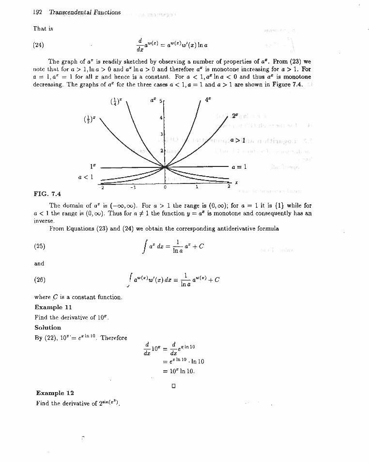
192 Tkmscendentd Functions
That is
The graph of az is readily sketched by observing a number of properties of aZ. From (23) we note that for a > 1, ln a > 0 and a" In a > 0 and therefore aZ is monotone increasing for a > 1. For a = 1 , a" = 1 for all z and hence is a constant. For a < 1, aZ ln a < 0 and thus a' is monotone decreasing. The graphs of a' for the three cases a < 1, a = 1 and a > 1 are shown in Figure 7.4.
FIG. 7.4
The domain of a" is (-oo,oo). For a > 1 the range is (0, m); for a = 1 it is (1) while for a < 1 the range is (0,oo). Thus for a # 1 the function y = aZ is monotone and consequently has an inverse.
From Equations (23) and (24) we obtain the corresponding antiderivative formula
and
.where ,C is a constant function.
Example 11
Find the derivative of 10"
Solution
By (22)) loz'= ex'" lo. Therefore d d - 10s = -@ 1" 10 dx dx
- ez In 10 - ln 10
= 10" ln 10.
Example 12
Find the derivative of 2dn(x2).
7.3 Logarithm and Exponential to Other Bases 193
Solution
BY (24)
Example 13
Given that
dat Take the natural logarithm of each side and use implicit differentiation to obtain -.
dx Solution
Taking the natural logarithm of each side of the equation gives
Now differentiate implicitly, keeping in mind that y is a function of x.
1 dy -- = Ina. Y dx
Thus
as before. This process of taking natural logarithm and then differentiating is called logarithmic difler-
entiation.
Example 14
Determine the antiderivative of xnza,
Solution
We need to find xn' d x . Let u = x2, then du = 2 1 dx. Consequently / =
1 1 = - . - nu + C by (25) 2 Inn

Example 15 1
Evaluate 4-# ds.
Solution
Let w = -2, then dw = -dz. When z = 4 , w = - 4 and when x = 1, w = -1. Thus
We now use the fact established earlier that for a # 1, y = a" is monotone to define its inverse.
DEFINITION The logarithm function t o any base 0 > 0 , denoted by log, is defined for x > 0 bg
(27) y = log, x af and only if x = aY
The domain of log, is (0, oo) while the range is (-m, 00).
0
The logarithm function defined by (27) satisfies the usual laws of logarithm. Thus
log, 1 = 0 log,(uv) = log, u + log, v
log, (t) = -log, u
and log, u' = r log, u for r real.
The-first of these laws follows readily from the fact that a0 = 1. To prove the second of these, let log, u = x.and log, v = y then u = a" and v = ar . Therefore
Now take logarithm to base a of each side:
logo(yv) = log, a"+'
= x + y = log, u + log, v .

7.3 Logarithm and Exponential to Other Bases 195
Derivative of log, x
d To determine - log, x for x > 0 we let y = log, z. Then x = a#. Differentiating this implicitly with
dx reapect to x we get
Thus
frorxi which it follows that
dy 1 1 -=-=- dx aulna x l n a
d 1 - log, x = - for x > 0. dx z ln a
For x < 0, log,(-x) is well-defined and if we let u = -x then
d d - log, (-2) = - log, u dx dx
- 1 du . - u lna dx
1 d(-X) =-.- -xlna dx
1 =- for z < 0 x In a
Thus
d 1 - log, 1x1 = - dx x l n a '
Example 16 d
Find - log2 x 4 dx
Solution
Alternatively, since log2 x4 = 4 log2 x,
Example 17
Find the derivative of log, I sin X I .
Solution
Let w = sin x then d d - logo 1 sin X I = logo lwl dx
- 1 -- . coax by (28) w ln a
- COB x - ainxlna cot x = -. In a
Example 18 d
Find -log8 1%' - 8~ + 11. dz
Solution
Exercises 7.3
Find the derivative of each of the functions in problems 1-8.
1 3" 2 4za 3 5 6
7 loglo l x 3 - 42 + 11 8 log5 x2
In problems 9-11 use logarithmic differentiation to find the derivative of the functions.
9 xZ, x > o 10 2 6 , z > O
11 U ( X ) " ( ~ ) where u and u are differentiatiable functions of z and u ( x ) > 0.
In problems 12-17 find the indicated antiderivatives.
18 Find the relative minimum of the function f ( z ) = 2' + 2". 19 Find the area of the region bounded by the coordinate axes, the graph of y = 2' and the line
x = 3.

7.4 Inverse lligonometric Functions 197
In problems 20-24 evaluate the given integrals.
24 1' sin x 1OCo8' dx
7.4 Inverse Trigonometric Functions
The inverse trigonometric functions arcsinx or sin'' x, arccoez or COB-' z, arctanz or tan-'z, arccscx or csc-I x, arcsecz or csc-' x and arccot x or cot-' x are defined in terms of the corre- sponding trigonometric functions by restricting the domain of such trigonometric functions to where the functions are monotone. Thus, for example, by limiting the domain of sine to [-5, $1 we define arcsin by
a s y=arcsinx i fandonlyif x = s i n y , yE[-l,I].
For a review of the inverse trigonometric functions see Section 5.5 of Volume 1. From the above definition of arcsin we may obtain D arcsin x. Differentiating the second
equation x = sin y implicitly with respect to x we have
1 = D, sin y = cosy . D,y.
That is D,y = &. But for y E [-s/2, n/2], cosy > 0 and is thus given by
cos y = Jz =
Therefore 1
Dz arcsin z = D, sin-' x = D,y = - d m . For determining D cos-' x we recall that
y = cos-' x if and oniy if x = cosy, y E [0, n].
Again differentiating the second relation implicitly with respect to x gives
and since sin y 2 0 for y E [0, s ] we have
sin y = dl-cos2y = d C 2 .
Hence

198 'Ranscenden tal Functions
The derivatives of the other inverse trigonometric functions may be derived in a similar manner. We summarize all these results below.
1 Dcot" x = --
1 + x2
Corresponding to each of the derivative formulas (29)-(34) is an antiderivative formula. These are
- tan" x + C or - cot" x + C J&- dx = sec-' x + C or - cec" x + C.
Example 19
Find D arcsin(x2 + 3).
Solution
Let u = xa + 3, then D arcsin(xa + 3) = D, arcsin u . Dtu
Example 20 - 0
Determine the cubic approximation to sin-' x at x = 0.
Solution
The cubic approximation to f (x) at x = 0 is (see Section 4.)
Take f (x) = sin- ' x, then

7.5 Hyperbolic and Inverse Hyperbolic Functions 199
Therefore
Hence
Example 21
Evaluate
Sohtion
Let x = 2v than d x = 2dv . When x = 2 , v = 1 and when x = 4, v = 2. Therefore
Exercises 7.4
1 Derive from the definition of csc-' x the formula (32).
2 Derive from the definition of cot-' x the formula (34). In problems 3-7 find the derivative of each of the indicated functions.
3 tan-' &G 4 sin-'(coe x) 5 csc-' (32 + 4)
6 (arcsin x ) ~ + (arccos x)* 7 COS-' (COS 22)
8 Find the critical point(s) of f (x) = sin-' x + 2 d 3 and classify the extrema.
Determine the cubic approximation a t x = 0 of e.ach of the functions in problem 9-11.
9 tan-' x 10 cos-'x 11 sin-' (sin x)
Determine the indicated antiderivatives in problems 12-16
17 Evaluate la d&, a>O.

Hyperbolic and Inverse Hyperbolic Functions
We ehall conclude this chapter by giving a brief diecueeion of the hyperbolic functions and invem hyperbolic functions.
DEFINITION The hyperbolic functions, sinh and coeh a n defined for real variable x by
1 sinh x = - (ef - e'*)
2 1
cosh x = - (e f + e") . 2
Since the domain of ef and e-* is (-00, oo) the domain of ccwh x and sinh x is also (-00, oo). The range of sinh x is (-00, oo) while that of cosh x is [l,oo). The graphs of these functions are sketched in Figure 7.5. Other hyperbolic functions tanh, coth, eech and csch are defined in t e r m of sinh and cosh as follows.
sinh z tanh x = -
cosh z cosh z
cothx = - sinh z x # 0
1 sech z = -
ccwh x 1
isch z = - sinh x ~ $ 0
A number of identities similar to those for trigonometric functions are readily derived from the definitions. Some of these are
cosha x - sinh2 x = 1
sinh(z f y) = sinh x cosh y f cosh x sinh y.
cosh(x f y) = cosh x cosh y f sinh x sinh y
FIG. 7.5

7.5 Hyperbolic and lnverse Hyperbolic Functions 201
From the definitions (29) and (30) it follows that
(32) ' d 1 - sinh x = - (eZ + e - = ) = cosh x dx 2
(33) d 1 - cash x = - (eZ - e-=) = sinh z dx 2
More generally, if w is a.differentiable function of x
d - sinh w ( x ) = wl(x) cosh W(X) dx d
and - cosh W(X) = wl(x) sinh w(x) dx
The corresponding antiderivative formulas are
I cosh z dx = sinh z + C
I sinh x d2 = cash x.+ C.
Example 22 d
Find - tanh x. dx
Solution sinh x
D tanh x = D- cosh x
- coshx. Ds inhx - sinhx . Dcoshx - cosh2 x
- cosh2 x - sinh2 x - cosh2 x
The derivatives of the other hyperbolic functions are derived using the quotient rule as donf in the example above. The results are as follows.
D coth x = -csch2 x
Dsech x = -sech x tanh x
Dcsch x = -csch x coth x.
T h e integral formulas cdrresponding to the above are
J sech2 x dx = tanh x + C
J csch2 x dx = - coth x + C
I, sech x tanh x dx = -sech z + C

202 fianscendental finctions
Since the sinh function is monotone increasing (Dsinhz = coehz > 0) it has an inveree. This inverse denoted by arcsinh is defined by.
y = arcsinh x if and only if x = sinh y.
The symbol arcsinh is sometimes denoted by sinh". Rom the above definition it follows by implicit differentiation of x = sinh y that
dy 1 = cosh y- dx'
But cosh y = dl + sinh2 y
from which it follows that
by (31). Therefore
The corresponding antiderivative formula ie
- arcsinh z + C. J&- Finally, if we restrict cosh y to y > 0 then it is monotone increasing and consequently has an inverse denoted by arccosh or cosh", and defined by
y = arccosh x, x > 1 if and only if x = cosh y, y > 0.
Again differentiating implicitly gives dy 1 = sinh y-. dx
But sinh y = d m by (31). Thus
Hence
The corresponding integral formula is then
- arccosh x + C. /&-

7.5 Hyperbolic and Inverse Hyperbolic finctions 203
Solut ion
Let u = d m , then
Example 24
S o h t i on
Let u = 3x then du = 3dx. Therefore
1 = - arccosh u + C 3 1 = - arccosh (32) + C. 3
Exercises 7.5
Derive the identity sinh 22 = 2 sinh x cosh x.
Derive the identity cosh 22 = 2 cosh2 x - 1.
Prove that sinh is an odd function and that cosh is an even function.
Derive the two identities following equation (31).
In problem 5-9 find the derivative of each of the given functions.
sinh(x2) 6 cosh(1n 1x1) 7 tanh&
d Derive the result - coth t = -cscp2 x.
&

In problem 11-16 find the itldicated antiderivatives.
17 Evaluate coeh x dx.
18 Evaluate l2 Miecellaneous Exercises
df Find - for f (x) = In I cos X I . dx df Find - for f =ln1tanx+secx) . dx
Find the derivative of each of the functions (i) f (x) = e m and (ii) f (x) = e'cmz
In problems 4-12 find the indicated integrals.
13 / cash3 r einh r d i

Met hods of Integration
8.1 Introduction
In Chapter 5 we learnt from the Fundamental Theorem of Calculus that
with C as an integration constant. Thus -integration and differentiation are operations inverse to each other. Consequently in that chapter and also in Chapter 7 we deduced the integrals of certain functions some of which are listed hereunder.
/ t anxdx=ln I secx1+C
J secxtanxdx = secx+ C
dx - sin-' x + C
We shall refer to the integrands in (1) - (12) above as standard integrands and may add to the list as necessary.

206 Methods of Integration
We now seek to develop systematic techniques by which a given integrand may be reduced to a form similar to one of the above or a combination of integrands for which the integration rules
and / k f (x) d r = k / f ( r ) dx, kconstant
may be used where each of f (x) and g(x) is one of the integrands in (1) - (12) above.
8.2 Method of Substitution
Recall that in Section 5.5 we introduced the idea of employing a change in the variable of integration from x to say, u. This changz simplified integrals of the form
where F' is one of the standard integrands. In this section we extend the techniques to cover cases where $ f (2) dx is reduced, after one or more substitutions, to the form S g(u) du where g is a combiliation of one or more of the standard integrands.
Example 1
Find / sin3 x cos2 z d t
Solution
Let u = coa x +- du = -sin x, dx. Hence
J sin3 z cos2 x dx = sin2 x coa2 x(sin x dx) J
0 Remark 8.1,
In Section 5.5 Example 24 we integrated sin3 x cos t by using either u = ein x or u = coa z . However, in the above example, the eubetitution u = sin x does not lead to a standard integrand. Indeed for a function of form sinm x cosn x, the eubetitution u = sin x (u = coa x) will reduce the integrand to a polynomial in u provided n (m) is odd. The case where both m and n are even will be discussed in Section 8.4. Example 2
Find .f sec x dx

8.2 Method of Substitution 207
Solution cos x
JseCzc-ix=/&= JXdx .
Let u = s i n s du = cosxdx. Hence
coe x dx du
1/2 1/2 1
= J + =] du since
But 1 + u 1 + sin x (1 + sin x)(1 + sin x) (1 + sin x ) ~ -= - - - - 1 - u 1-s inx (1-s inx) ( l+s inx) cos2x '
TherEfore 1 1+ 1 (I + ~ i n x ) ~ -In - =ln laecx+ tanx l . 2 I l - : ( = H 1 " ( C O S ~ X ) = l n l cosx I
/ secxdz = In (secx + t anxl+ C.
The examples above indicate that some restructuring of an integrand may be necessary before a useful substitution becomes apparent. However, there are some classes of functions to which the method may be successfully applied.
(i) Funct ions of the fo rm F(ax + b): Let f , F be functions such that f(x) = F(ax + b) where a , b are constants. An appropriate substi- t u t i o n i s u = a x + b = = + d u = a d z , s o that
Example 3
Find J cos(3x + 5 ) dx.
Solution
Let u = 3x + 5 3 - d u = 3dx. Hence

208 Methodsoflntegration
Example 4
Find J(4 - 3x)'l7 dx.
Solut ion
Let u = 4 - 3x du = -3 dx and dx = -4 du. Therefore
(ii) Funct ions of t h e fo rm F ( d a x 2 + bx + c), a # 0. dz.
In Example 29 of Section 5.5 we noted that - I dT=2 could not be reduced to standard form by
substituting either u = 4 - x2 or u2 = 4 - x2. It will still be useful to eliminate the radical by expressing 4 - x2 as the square of some function. This can be achieved by either of the trigonometric functions sine or cosine. The substitution x = 2sinu which implies dx = 2cosu du, makes 4 - x2 = 4 - 4 sin2 u = 4 cos2 u = (2 cos u)' . Hence
dx 2 cos u du Jm= J fcosu = / ~ I L = ~ + C x = sin-' - + C 2
More generally for a function ~ ( d a x ~ + bx + c) we need to eliminate the radical by expressing ax2 + bx + c as the square of some function. The quadratic ax2 + bx + c reduces to one of the three forms A(k2 - u2), B ( U ~ - k2) and C(u2 + k2) with A, B , C positive and u = x + &. Note that ax2 + bx + c 2 0 for the square root function to exist.
For the form k2 - u2, the substitution u = k sin 8 (or u = k cos 8) reduces the form to k2 cos2 8 (or k2 sin2 8) as for 4 - x2 above.
For the form u2 - k2, the substitution u = k sec 8 (or u = k cosh 8) reduces the form to k2 tan2 8 (or k2 sinh2 8).
For the form u2 + k2, the substitution u = k tan t9 (or u = k sinh 8) reduces the form to k2 sec2 8 (or k2 cmh2 8).
These Abstitutions are usually called trigonometric (or hyperbolic) substitutions. The trigone metric substitutions are also called circular substitutions.
Example 6
dx Find I ,,- where a, b are non-zero constants.
Solution
The expression under the radical sign is of the form k2 - ua. Hence by letting u = ksin 8, say, we
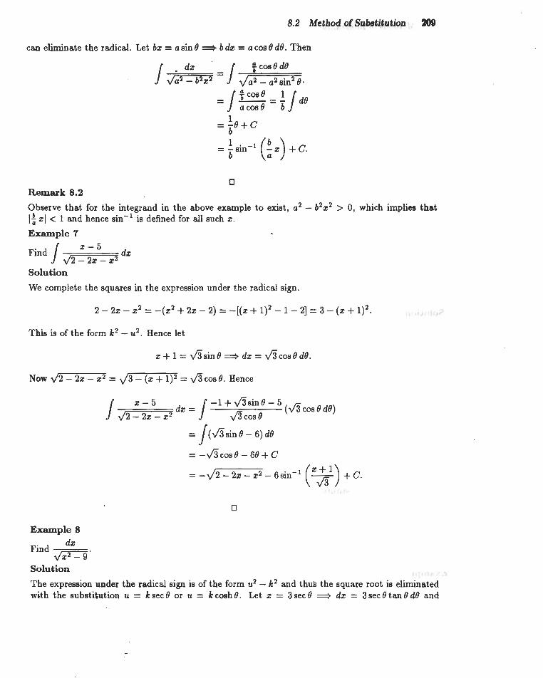
8.2 Method of Substitution 209
can eliminate the radical. Let bz = a sin 8 =+ b dz = a coa 8 do. Then
0 Remark 8.2
Observe that for the integrand in the above example to exist, a2 - b2z2 > 0, which implies that 1; X I < 1 and hence sin" is defined for all such x .
Example 7
Find / x - 5 dx
4 2 - 22 - 2 2
Solution
We complete the squares in the expression under the radical sign.
This is of the form k2 - u2. Hence let
NOW ,,2 - 2x - x2 = d m = ficos8. Hence
x - 5 - l + f i s i n 9 - 5 ( fi cos 8 do)
Example 8
Solution
The exprwion under the radical sign is of the form u2 - k2 and thub the square root is eliminated with the substitution u = k sec 8 or u = k coah8. Let x = 3 see 8 a dx = 3sec 8 tan 8 d8 and
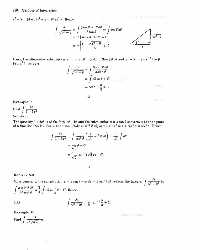
210 Methods of Integration
x2 - 9 = (3sec ~ 9 ) ~ - 9 = 9 tan2 8. Hence
Using the alternative substitution x = 3 cosh 0 dx = 3 sinh 0 d0 and x2 - 9 = 9 cosh2 0 - 9 = 9 sinh2 8, we have
dx 3 sinh 0 d0 /-=I 3sinhO
= / ~ o = B + c x = cosh-' - + C. 3
Example 9
Solution
The quantity 1 + 5x2 is of the form u2 + k2 and the substitution u = k tan 0 converts it to the square of a function. So let Ax = tan 8 =+ 6 d x = sec2 Ode, and 1 + 5x2 = 1 + tan2 8 = sec2 8. Hence
Remark 8.3
More generally, the substitution u = k tan 8 --r du = ksec2 8 dB reduces the integral
1 / kaec20d8 - i / d 8 = - O + C . Hence k2 sec2 0 - k k
Example 10

8.2 Method d ~ u b s t i t u t i o n 211
Solution
We try to eliminate the radical by substituting x = 2 tan8 a dx = 2sec2 8d8 and 4 + x' = 4 + 4 tan2 8 = 4 sec2 8. Hence
1 x 2 ~ - = 1 4 tan2 0(2 sec 0)
Example 11 4x+ 1
Find / d7 dx. x + x + l
Solution
Since x2 + x + 1 = (x + a)2 + $, the expression under the radical sign is of the form u2 + k2 and the substitution u = k tan 8 eliminates the radical sign. Let
Hence
42 + 1 dz = / 4(-i + tan 0) + 1 . - 4 sec2
9 sec 8 2
= /[-see8 + 2JjsecOtanO]dO
= - l n ( s e c 8 + t a n 8 1 + 2 & s e c O + ~ %
Exercises 8.2
Find each of the integrals in problems 1-12.

212 Methods of Integration
Evaluate each of the definite integrals in problems 13-15.
J sin2 x C O S ~ x dz.
8.3 Method of Partial Fractions
The method of partial fractions is a useful tool for integrating rational functions-the ratio of two polynomial functions. Let p, q be polynomial functions of degrees n, m respectively. The rational function r = is said to be proper if n < m and improper otherwise. If the rational function r is improper (i.e. n 2 m), by division r may be expressed as the sum of a polynomial and a proper rational function. That is,
where s = n - m, degree of g is less than m, and bo , bl , . . . , b, are constants. The integral of the polynomial part bo + blx + ... + b,xd above is in standard form. So t o be
able t o integrate J r(x) dx we need only determine how to integrate the improper rational part of r . This is achieved by expressing # as a sum of partial fractions. The basis for this is the following result (see Section 3.2 of Volume 1).
Let be a proper rational function with
Every such polynomial function q(x) can be written as a product
where the x - ai for i = 1 ,2 , . . . , k and x2 + pjx + 7, for j = 1,2,. . . , t are all distinct. For each i and j , (x - at),- and (x2 + Pjx + are the highe4 power of x - ai and x2 + Pj x + y, respectively that divide q(x). Also sl + s2 + + s k + 2(rl + r2 + rt) = rn. Each quadratic factor has no real roots, that is, it cannot be factored. Thus for each j, j = 1,2, . . . , t , @ - 4yj < 0.
Assign to (x - a i ) ' ~ the sum of si partial fractions
where Aij, j = 1,2, . . . , si are conetants.
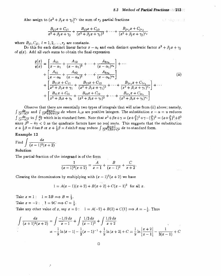
8.3 Method of Partial Frections 213
Also assign to (x2 + Pjx + 7,)'j the sum of r, partial fractions
where Bjl, Cjl , I = 1,2,. . . , rj are constants. Do this for each distinct linear factor x - cri and each distinct quadratic factor x2 + Pjx + 7j
of q(x). Add all such sums to obtain the final expression
( ii)
Observe that there are essentially two types of integrals that will arise from (ii) above; namely,
J & and J dx where A, p are positive integers. The substitution x - o = u reduces
1 & to J $J which is in standard form Note that x ~ + + ~ x + ~ = ( ~ + $ ) ~ + 7 - ( k ) ~ = ( ~ + f ) ' + 6 ~ since P2 - 47 < 0 as the quadratic factors have no real roots. This suggests that the substitution x + $0 = 6 tan t9 or x + = 6 sinh t9 may reduce J dx to standard form.
Example 12
Find / dx
( x - q 2 ( x + 2 ) Solution The partial fraction of the integrand is of the form
1 A B C -- +-+- ( x - 1)2(x+2) - x - 1 ( x - 1 ) 2 x+2'
Clearing the denominators by multiplying with ( x - 1)2(x + 2 ) we have
1 = A(x - 1)(x + 2) + B(x + 2 ) + C(x - 1)2 for a11 x.
T a k e x = l : 1 = 3 B * B = a .
Take x = - 2 : , 1 =9C*C= i. Take any other value of x, say x = 0 : 1 = A(-2) + B(2) + C(1) j A = -;. Thus

214 Methods o f Integration
Example 13
Find / 5x3 + 172 - 7 dx.
(x2 + 4)(x - 1) Solution
The integrand is improper since the degree of its numerator equals that of the denominator, namely 3. Therefore we must carry out a division first before resolving into partial fractions. Now
Let 5x2 - 3x + 13 - - A B x + C +- . Clearing the denominators, we obtain (x2 +4)(x - 1) 2 x2 + 4
5x2 - 33: + 13 = A ( X ~ + 4) + (Bx + C)(x - 1).
Take x = 1 : 15 = 5A d A = 3.
Equate coefficients of powers of x.
x 2 ; 5 = A + B a B = 2 .
x : - 3 = - B + C * C = B - 3 = - 1 .
Check Constant (xO) : 13 = 4A - C(= 12 - (-1)). Thus
and 5x3 + 17% - 7 (x" +)(x - 1)
Now let x = 2 t a n 8 ~ d x = 2 s e c 2 8 d 8 , so that
Therefore

8.3 Method. f Pardid Ractions 216 P Example 14
x4 + 4x2 + 42 - 5 lind J ( x + 3)(x2 + z +4)2 dx' Solution
x 4 + 4 x 2 + 4 x - 5 A B x + C D x + E -- ( x + 3)(r2 + x + 4)2 - x + 3 + x2 + 2 + 4 + ( x2 + x + 412 ..
On clearing denominators we obtain
x4 + 4x2 + 4~ - 5 = A ( X ~ + z + 4)2 + ( 8 2 + C ) ( X + 3)(x2 + x + 4) + ( D X + E)(Z + 3)
= A ( X ~ + 22' + 9x2 + 8% + 16) + [Bx2 + (3B + C ) x + 3 q ( x 2 + z + 4) 4 I ~ X + EI (X + 3)
Take x = -3 : 100 = A(10)= A = 1
Equate coefficients of powers of x .
Constant: -5 = 1 ' 6 ~ + 12C + 3E j E = ;(-5 - 16A - 12C) = 1. Hence
and
1 Let z + . ~ = ~ t a n 6 ~ d x = - \ / i j s e c 2 6 d 6 . S o 2 2 2
The substitution u = sin 6 reduce# $ lin 6 cos 0 d6 to J u du = !p2 = 4 sin2 6 = i (e) x +1+4 '

216 Methods of Integration
Methods for finding cos2 0 dB will be discussed in the next section. Thus
so far.
a
Exercises 8.3
Find each of the integrals in problems 1-14
Methods for Trigonometric Functions
In this section we present methods of integration which are based on the structure of trigonometric functions.
8.4.1 Integrands of the form sin a x cos bx, sin a x sin bx, cos ax cos bx
The integration of the above products is based on the addition formulae
cos(Af B) = c o s A c o s B ~ s i n A s i n B
which lead to the product formulae
1 sin P cos Q = -[sin(P + Q) + sin(P - Q)]
2 1
sin P sin Q = ;i[cos(P - Q) - cw(P + Q)]
1 coe P cos Q = - [coe(P - Q) + cw(P + Q)].
2

8.4 Methods for Tkigonometric hnct ions 217
Thus, for example,
sin ax cos bx dx I -[sin(a + b)x + sin(a - b)x] dx J : Each of the two integral8 on the right hand side can be readily obtained by the substitution method.
Example 15
Find J sin 32 sin x dx.
Solution
sin 3x sin x = ;[cos(3x - x) - cos(3x + x)] = $ cos 22 - cos 4x. Hence
sin 32 sin x dx =
Example 16
Find (i) J cos2 x dx (ii) Jsin2 x dx.
Solution
(i) cosa x = &(I + cos 22). Therefore .
(ii) sina x = $( I - cos 22). Thus
8.4.2 Integrande which are rational functions of a cos x + b sin x
We note that these integrals are of the form .r r(x) dx with r a rational function o if u = acosx+bsinx. Since we know how to integrate rational fuktioks with respect to their variable, we seek to reduce J r(x) dx to J R(t) dt where R is also a rational function. This can be achieved by the substitution t = tan $.
Recall that sin z = 2 sin 5 cos $ and cos x = cos2 $ - 8in2 $. Dividing each identity by 1 = cos2 5 + sina $ we have
2sin $ cos $ - 2 tan % sin z = - and
cos2$+sin$ l + t a n a $
1 - tana 5 cosz =
1 + tan2 5 '

218 Methods of In tegrat i o~
21 1-12 Thus sin z = -
1 + t 2 and cos x = - 1 + t2. *Iso
Hence
Example 17
Find / dx 5 + 4 c o s x '
Solution x 2 dt
Let t = tan - a dx = - 2
; ::. Hence and also cos z = - 1 + t 2
Let t = 3tanQ a dt = 3sec2QdQ. ~ h u s
Therefore
I dx 2 = -tan-' ( 5 tan 5 ) + C. 5 + 4 c o s x 3
a Example 18
Find / dx 1 +3sinz.+ cosz '
Solution x 2 dt
Let t = tan - a dx = - 2
+ t2 . Hence ,

8.4 Methods for 'fl.gonometric finctions 219
Example 19
Find I = 1 5 - t 2 x a
Solution
Solving we obtain A = 0, C = 0, B = and D = ' . Hence 5r 9
0 Remark 8.4
Note that the integral, I, may be written as
for which an appropriate substitution is t = tan x.
Exercises 8.4
Find the each ofethe integrals in problems 1-9.
1 J sin 5z cas 3x dx 2 J cos 2x cos 7x dx 3 j cos2 4x dx
. . 4 Jsin2 2xdx ' 5 Jcos2 5x 6 /sin a x sin 3z dz

220 Methods of integration
Evaluate the definite integrals in problems 10-15. In problems 13 and 14 consider the cases m = n arid m # n separately.
13 ~ ' s i n m x s i n n x d x 14 lr cos mx cce nx dx 15 lr sin mx ro i nx dx
8.5 Integration by Parts
Each of the integrands we have dealt with so far has been one of the following six function types, namely
trigonometric functions inverse trigonometric functions exponential functions logarithmic functions polynomial (and rational) functions hypcrbohc functions.
IIowever, thcre arc natural pheonomcna whose mathematical description involve products of these function types. For exarr~ple, t.he product e-W'sin(at +a) , where t represents time and w , a, a are constants, describe damped oscillations as are to be found when a pendulum oscillates in a resistant medium, a guitar string is plucked, or a stone is dropped into a pool of water. It is therefore useful to derive methods for obtaining integrals of functions which are products of two (or more) of the six function types listed above.
Consider the rule for the differentiation of a product u(x)v(x) of two functions u(x), v(x) of a variable x; that is,
d dv du -(uv) = u- + v- dx dx dx"
If we integrate each side of this equation with respect to x , we'obtain
which gives
Equation (15) indicates one integral on each side of the equality sign. These integrals are of the same general form except that the roles of u(x) and v(x) are interchanged. The process above is called rntegratron by parts. It is useful when the right hand side integrand is easier t o reduce t o standard form (and-thus involving only one of the six function types) than the left hand side integrand.
We shall apply this method to the integration of products of two of the six function types listed above where u(x) and are any two of such functions. Note that by expressing the integrand as a product of form u(x)% we imply that v is known; that is, the second factor in the product is a derivative of a known function.

8.5 Integration by Parts 221
Example 20 . Find 1 re3" d x .
Solution
For this integrand we know how to integrate both x and e3" and so either can be $. Chozce 1:
d v 1 u = x, - = e32 v = -e3", Therefore
dx 3
Choice 2: d v 1
u = e3" - = x a v = - x 2 . Therefore . ' d x 2
The integrand on the right hand side is still of the same form as the original integrand except that the index of x is now higher. So Choice 2 does not help.
Remark 8.5
In integrating to obtain v ( x ) we do not include a constant of integration K, say. If we add this to v ( x ) we obtain
= uv - v - d x as before. / 2 Find J x2 sin x d x .
Solution d v
~ e t u = x 2 , - = sinx -4 v = -COSX. Therefore dx
x2 sin x dx = x2 ( - cos x ) -

222 Methodsof Integration
At this point we have reduced the power of x from 2 to 1. A repeat of t$e procedure on S x cos x dx will further (we hope) reduce the power of,x from 1 to zero.
du Let u = x, - = cos x =+ u = sin x. Therefore
dx .
1 I xcosxdx=x(s inx)- s inx .1dx
' = xsinx - (-cosx).
Thus
Example 22
Find $zn Inxdx , n f - 1 .
Sorution
Here we do not, yet know the integral of h i . Hence $ must be chosen equal to xn . So let dv
u = i n x , - - = X " - V = - - xn+', n + 1 # 0. Therefore dx n + l .
Remark 8.6
(i) For the case n = 0, the above resu!t reduces to
(ii) The example above for the cme n = 0 irn&ies our choosing g = 1, that is identifying l n z a. 1 . ln x. This idea is often useful when we have an integrand of one function-type alone which is not amenable to the other methods ,of integration.
Example 23
Find Jain-' x dx.
Solution du
Let u(x) = sin".x, - = 1 =+ u = x. Therefore dz

8.5 Integration by Parts 223
For the integral set z = 1 - x2 a dr = -2x d x , Therefore
Thus
Example 24
Find I = d m ' d x where a is a non-zero constant.
Solution dv
We set u = dm and - = 1 -4 v = x . Therefore dx
x2 d2 . x2 x? + a2 - a2 To find / dr, we note that -- - a2
- Thus
a + +
Therefore
aa where K = C + + In 1.1 = constant.

224 Methods of Integration
Example 25
Find I = $ ear cos bx dx.
Solution dv 1
Let u = ea" - = cos bx 3 v = -sin bx. Therefore ' dx b
I = e" (t sin bx) - / t sin bx(aea') dx
0)
We observe that neither ea' nor cos bx can be eliminated: ear remains the same but cos bx is changed to sin bx. Therefore a repetition of integration by parts will transform ea" sin bx to ear coe bz and we can thus have an equation involving I.
dv 1 Let u = ear - = sin bx a v = -- cos bx. Therefore ' dx b
/ ear sin bx dx = eax (- ; cod bx) - / (- f coa bx) aeax dx
Hence substituting back into (i) we have
Thus
1 a a2 = -ea" sin bx + -ea" cos bx - -I + C
b b2 b2
I bx -+ a cos bx)em + C
and I = - I eax(b sin bx + a cos bx) + K
a2 + b2
C where K = - a2 + b2 - - constant.
0
Exercises 8.5
Fivd each of, the integrals in problems 1-18. '
/ z2 sin x dx
/."nzdz
/ c o s ~ ; d z

Evaluate each of the definite integrals in problems 1
x tan-' x dx
Reduction Formulae 225
/ x2eaz dx.
1=14 xsinxcosxdz
8.6' Reduction Formulae
In this last section of the chapter we discuss the application of the method of integration by parts and other integration techniques to the derivation of integrals of powers of trigonometric, logarithmic and algebraic functions in terms of similar integrals with lower powers of these functions. Specifically we seek S(U(X))" dx in terms of S(u(x))"-l dx or J(U(X))"-~ dx where u(x) is either a trigonometric, logarithmic or algebraic function. Such a relation is called a reduction formula.
8.6.3 Reduction Formulae for S sinn z'dz and S cosn x dx for n 2 2
du Now S sinn x dx = S sinn-' x sin x dx. We integrate by parts: Let u = sinn-' x, - = sin x =+ u =
dx - cos x. Therefore
sinn x dz = sinn" x(- cos x) - (- cos x)(n - 1) sinn-' x COB z dx
= - sinn-' x cos x + (n - 1) / (1 - sin2 x) sinn-l x dx
= - ~ i n " - ~ x c o s x + ( n - l)In-' - ( n - l )In
i.e., nIn = -sinn-' x cosx + (n - 1)In-2 or
J 1 n
n - l /sinn-'xdx n 2 2 . &inn xdx = '-sinn-' icos;e + - n
Simialrly 1
cosn x dx = - cosn" *sin x + - n n l J c o s x x n n 2 2 .

226 Methods of Integration
8.6.4 Reduction Formulae for I(m, n) = S sinm z cosn z dz for n, m 2 2
dv We integrate Z(m, n) = S sinm z cosn z dz by parts by setting u = cosn-' z = sinm z cos z a
I
u = - sinn+' z. Therefore n+1
1 I (m, n) = COP-' sinm+' z[(n - 1 ) COS"-~ z(- sin z ) ] dz
m + l
- . 1 n - 1 n - 1 -- ccsn-' z sinm+' z + - Z(m, n - 2) - -Z(m, n) m + 1 m+1 m+1
By combining the two terms in I(m, n) a n d solving we obtain
1 n - 1 I(m, n ) :-I cosn-' z sinm+' 3: +- --1 (m , n - 2)
m + n m + ?a
J 1 sinm t cosn t d x := - 1 cosn- 1 x + - - ' /sinm r cosn-? r dr.
m -t n m + n dv By using u = sinm-' z , - = cosn z sin z we obtain the alternative reduction formula dz
J 1 z cos"+l 2 + -. sinm t cosn t d t = - - m L 1 / ~ i n ~ - ~ r c o e " z d z . m + n m + n
Example 26
Find S sin2 t t o s 4 z d t . Solution
I(m, n) = S sinm t cos" t dz. Since m =: 2, n = 4 we use the formula which reduces m. That is,
Thus
But by Subsection 8.6.1 above
, Thus 1 3 I4 = - c0s3 t sin t + -I2
4 4

8.6 Reduction Formulae 227
Therefore 1(2,4 j = J sin2 x c08x dx
+ C
1 1 1 1 = --sinzcossz+ -cos3x.sinz+ -coszsinz+ -Z+C. 6 24 16 16
8.6.3 Reduction Formulae for. $ tann z dz and $ cotn z dx for n 2 2
Let In = $ tann x dz. Then
= ] un-2 dy - In-2 where u = tan z with du = aec2 z dz
That is, for n > 2, 1
tan" x dx = -- J tann-" z - tann-' x dx. n - 1 J
T h w by repeated use of this formula we can find $ tann 2 dz for n = 2,3,4, . . .. By a similar derivation we obtain the following result
for n = 2,3,4 ,.... Example 27
Find $ cot6 z dx.
Solution Let la = $ cot6 z dz. By the reduction formula,
Therefore 1 1
la =--c0t4z- I ~ = - - c o ~ ~ ~ - 4 4
- 1 1 J ---cot4z+-cota.+ cotzdz ' 4 2

228 Methods of Integration
8.6.4 Reduction Formulae for $secn x dx and $ cscn z dx for n > 2
dv - Let In = $ secn x dz = ~ e c " - ~ z sec2 x dz. We integrate by parts using u = seen-' x, - - dz
sec2 2 v = tan z. Therefore
= s e ~ " - ~ z tan z - (n - 2) / awn-' z(sec2 z - 1) dz
= ~ e c " - ~ z tan x - (n - 2)In + (n - 2)In-2
That ie (n - l)In = s e ~ " - ~ z tan z + (n - 2)In,2, and thus
/ 1 secn z dx = - secn-2 x tan z + -
n - 1 n - 1 n - 2 Jsecn-2xdx n 2 2 .
Similarlv 1
cscn 2 dz = -- C S C ~ + ~ z cot z + - n-2/cscn-2xdx n > 2 . n - 1 n - 1
0 Example 28
Find $ d m d x where a is non-zero constant.
Solution Put x = a t a n 8 ~ d z = a s e c 2 8 d 8 then
J J=,~z = 1 asec 8(a sec20 do) = 2 see3 8 do. / Let Is = $ sec3 8 dB. By reduction formula
Thus
Hence
1 1 where K = a2C + -a2 ln 1-1.
2 a

8.6 Reduction Formulae 229
See eleo Example 24.
0
8.6.5 Reduction Formulae for $ secn z tanm z dz and $ cscn z cotm z dz for m, n > 2
Let ~ ( m , n) = S aecn z tanm z dz = $ secn-' z tanm-' z(sec z tan z) dz. To integrate by parts we set dv
u aecn-' 2 tanm-' z , - = eec z tan z 3 v = sec z. Therefore dz
Z(n, rn) = J k c n z tanm z dz
= secn-l tanm-' =(set 2) - sec x[(n - l ) ~ c " ' ~ z tanm-' z sec z tan z J
Thus (n + m - l)Z(n, m) = secn z tanm-I z - (m - l)Z(n, m - 2) or
1 m - 1 I(n,m) = secn x tanm'' z - Z(n,m - 2)
n + m - 1 n + m - 1
that is
By method of derivation the above result is valid for all n, m 2 1 so that dv = sec z tanx exists. dv
By using u = secnm2 z tanm z , - = sec2 z as in the integration of Ssecn xdz in Subsection 8.6.4 dz
above, we obtain an alternative reduction formula in which the index of sec x is decreased, namely
1 n - 2 Z(n, m) = secn-2 z tanm+' z + Z(n - 2, m).
n + m - 1 n + m - 1
Or J secn z tanm x dx = 1 secn-2 z tanm+' z -
n + m - 1 n + m - 1 n - 2 Jsecn-'xtanmzdz.
By method of derivation this requires n 2 2, m 2 1. By method similar to the above we can obtain
for n ,m 3 1 and
for n 3 2, m > 1. . .

230 Methods of Integration
Example 29
Find J tan2 I9 sec I9 dB.
Solution For I(n, rn) = f see 8 tan2 8 dB only 9 = sec I9 tan I9 is possible as indexfof sec 8 is one. By reduction formula
1 rn-1 ~ ( n , m ) = =cn 8 tanm" 19 - I(n, m - 2).
n + m - 1 n+m-1 We haven = 1, m = 2 s o that
0
8.6.6 Reduction Formulae for J(ln z)" dx n 2 1
du ,
We integrate by parts: Let u = (In z)", - = 1 a v = z . Therefore dx
1 In = z(ln x)" - / 2 n(ln .)"-I - dx
2 .
= +(In 2)" - nI,.,-l
8.6.7 Reduction Formulae for 1 (x2 Fk2)n 2
We encountered the above integral in Section 8.3 on the method of partial fractions. We use inte- 1 dv
gration by parts. Let u = + k2)n , - - l a v = x a n d - dz
Now x2 - (z2 + k2) - k2 ' 1 ' - kZ
(x2 + k2)"+l - (x2 + k2)n+l .= ($ + k2)n ( t 2 + k2)n+1 '
Therefore x dz
In = (x2 + k2)" + 2n [/ (x2 + k2)" - k2 / ( ~ 2 + dz k2)"+1 1

8.6 Reduction Formulae 231
Replacing n by n - 1, we have
1 x The repeated use of this formula reduces In to an expression involving Il = - tan-' -
k k
Exercises 8.6
Find each of the integrals in problems 1-9.
1 /sec4 xdx / cos6 x dx 3 / sin4 x dx
4 /tan7 xdx
10 Evaluate s;l2(sin 4 + cos2 4)2 d4.
11 Obtain a reduction formula for S xn cos x dx and use it to find S x3 cos x dx.
12 Obtain a reduction formula for S xn sin ax dx and use it to find J x4 sin 2 x dx . xn
13 Find a reduction formula for / dx where a is a constant. Use your relation to find
x5
14 Find a reduction formula for /(%' + a2)* dx where a is a constant.
1 15 If Pn = So xn cos nx dx and n is a positive integer greater than 1, show that n2Pn + n + n(n - 1)Pn-2 = 0.
1 16 If Pn = s:,'/' x cosn x dx, where n is a positive integer greater than 1, show that Pn = --
n2 +
n-1 - Pn-2. Evaluate Pa. . . n
' 'Derive the reduction formula for each of the integrals in problems 18-20 given in the text.

Miscellaneous Exercises Find each of the integrals in prdhlkins 1-24.
Evaluate the definite integrals in problems 25-33.

Answers to Exercises
Chapter 1
Exercises 1.2 (Page 9) 2 Same
3
Id 4 No. -(x) is not defined for x > 0.
mod 5
9 Neither except when denominator is a constant function. In this c&e?the quotient is a linear function.
10
f p , = 5 '1L f (z) = 22 - 1
i '; _-------------....- --.-
-a -2
.-------------...------I

range(r) = (-oo,~) u (0,oo).
Exercises 1.3 (Page 12) 1 12+21
3 cos (a!('
5 lzl,same'asf
7 1x1, same as h
10 No
14 No.

~xercises 1.4 (Page 15)
Answers to Exercises 235
sin-' t
Exercises 1.5 (Page 15) 1 R 2 (-m, -1) U (-1, W)
236 Answers to Exercises
5 R+
Miscellaneous Exercises (Page 15) .-
f + g = ( a + ~ ) z + b + d ; f l g = %; glf = 3; f -g = acza+(ad+bc)z+bd; dam ( f +g) = R, range (f + g) = R, dom (flg) = R - (-9, range (fig) = R - dam (!?If) = R-{-a>, rmge(g/ f )=R-{; ) , d o m ( f g ) = R , r ange ( fg )=R.
f o g = -7-4121; 9 0 f = 11-421+2, g ~ g = 121-k.4.
mod o mod 4%) = mod (2).
No, f (0) = 0 while f (z) = 1 for z # 0. f-'(2) = z'I3
n = 0 , 2 . For n = 0 f . f = 1, while for n = 2 f . f = z 4 .
R - {-3,3) 8 ( - 0 0 , - l ) U ( 2 , ~ )
R - (-1, 1} 10. (-00, -45) u [-I, 11 u (45 , 00).
Chapter 2
Exercises 2.1 (Page 20) 1 3
Exercises 2.3 (Page 33) 3 3
4 6 a. - b. no limit
3

Answers to Exercises 237
Exercises 2.4 (Page 39) 1 (i) - 1 (ii) 1 (iii) no (iv) 0 (v) 0 limit (vi) 1
2 0
3
Limits are 1, 1 and 1 respectively.
4 -1 5 -1
Exercises 2.6 (Page 44) I No. f (5) is not defined.
2 (i) Yes (ii) Not continuous, left and right limits are not equal (iii) Not continuous, left and right limits are not equal
3 . Yes
4 (i) removabk, f * (3) = 6, f' (x) = f (x), x + 3 (ii) removable, f.(g) = 8 (iii) essential discontinuity, lim,,9 does not exist. (iv) essential discontinuity, 8 =. limZd4- # lim,,4+ = -28 (v) essential discontinuity, lim,,9- # lim,,g+
5 2
6 None.

238 Answers to Exercises
Exercises 2.7 (Page 50) 1 Cannot conclude based on theorems. No, by solving.
2 Cannot conclude based on theor'ems. No, by solving.
3 Yes. f(O)f(2)<0
4 Yes. f (1) f (3) < 0
5 Yes.Infacttwoaolutions.z=l andxE[-1,0]
6 [-2, -11
7 [-1,01 8 2, f (- 1) f (0) < 0 and f (1) f (2) < 0. Note that f (2) = a
9 None. Note that f (x) = 2x2[(x + + $1 + 1 > 1 for all x.
Miscellaneous Exercises (Page 50)
2 (i) (ii)
Chapter 3
Exercises 3.2
1 3x2
Exercises 3.3
Exercises 3.4 1 secz tanx
4 -asin(at)
1 3 (i) -1 (ii) 12 4 (i) 4 (ii) 0
6 Yes 7 Yes
9 Yes 10 (-3,-2)
(Page 56) 1
2 -- t a
6 -1
(Page 58)
(Page 60) 2 - c e c t e o t t

' . Answers to Exercises 239
Exercises 3.5 (Page 68) 1 - 6 ~ ' ~ 2 - 6 ~ - ~ + 4 ~ - ~ 3 2nxan-I + 2nanxn'"
4 s inx + x cos x 1
5 nxn-' + ( n + -)xn-4 6 cosx 2
I + & 7 -- 8 3 + ~ + 8 x - ~ 9 22 + 15x4 + 7x6 x2
1 10 sin x + see x tan x 11 3x2cosx - x3s inx 12 -(x - 1)(5x - 1)
2 6
13 l + x
14 2 see2 x .
15 -1 + 4x - 2x2 + 8x3 + 2x4 + x6
2&(l - x)a ( 1 - tan x ) ~ ( 2 + + x3)2
17 -5 cos4 x sin x
19 3a(az - b)2 20 I ~ X ( X ~ - 115 1
21 3x2 - 8x- ' /6 - 3x-4
22 ( i ) and (ii) cos 21 23 4 + 15%' + 5x4 24 5x4(1 - cos x ) + xS sin x
25 z c o s x - s inz
2 2
7 cos x 26
(4 + 3 sin x)2
Exercises 3.6 (Page 71) 1 15(3x + 4)4 2 16x(1 - 2xa)-5
5 24x(1+ 4 ~ ~ ) ~ cos(l+ 4 ~ ~ ) ~ 4 :x(x2 + 2)-2/3 cos V;?Ti
7 x ~ ( 1 - ~ ) ~ ( 4 - 7 ~ ) 8 lO(3sin 21 + + cos 7 ~ ) ~ ( 6 cos 22 - 7 sin 7 2 )
1 1 9 3(x2 + ; - tan 2x)'(2x - - - 2sec2 22) 10 6x(1+ 0 ~ ) ~ ( 1 - 22)-4 + 8x(1+ x2)8(1 -
x2
11 2x(3 - 52 + 3x2)
2
4 3 - 4x + 2x2
13 4 ein(2 cos 22) sin 22
12 sec2(sin x ) cos z
14 cos[sin(sin x)] cos(sin x ) . cos x

240 Answers to Exercises
Exercises 3.7 (Page 74)
Exercises 3.8 (Page 77)
Exercises 3.9 (Page 83)
5 -- 2
3 3 -- and - 2 2
1 2 ( 4 ~ + 5 ) ~ , 96(4x+5) 4 a cos(ax + b), -a2 sin(ax + b)
a4 cos(ax + b) 8 24xsec2 u tan u + 16x3 sec2 u[l + 3 tan2 u], u = x2
4 1-cos2x 19 -
3 (sin 8 - sin 36)3

Answers to Exercises 241
24 27 sin3 x - 20 sin x
Miscellaneous Exercises (Page 84)
7 72x3(3x4 + 5)' 8 14 sin 7 x cos 7 x
9 - sin(sin x ) cos x
s iny - y s i n x 12 -
x c o s y + cosx
18 24(2x + 1 ) (x - 4)4 + 48(2x + 1)'(x - 4)3 + 12(2x + 1)'(x - 4)'
19 2 sec2 x ( 1 + x tan x ) 20 144(24x - 23 ) .
Chapter 4
Exercises 4.1 (Page 89) 1 y = 3 x - 2 2 1 : + 2 y = 3
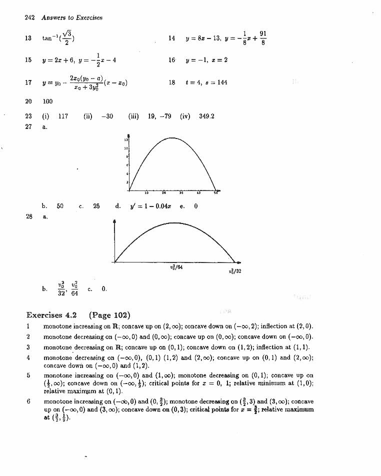
242 Answers to Exercises
23 (i) 117 (ii) -30 (iii) 19,-79 (iv) 349.2
27 a.
Exercises 4.2 (Page 102) monotone increasing on R; concave up on (2,oo); concave down on (-oo,2); inflection at (2,O).
monotone decreasing on (-oo, 0) and (0,~); concave up on (0, oo); concave down on (-00, 0).
monotone decreasing on R; concave up on (0,l); concave down on (1,2); inflection at (1,l).
monotone decreasing on (-m,O), (0,l) (1,2) and (2,~); concave up on (0,l) and (2,oo); concave down on (-oo,O) and (1,2). monotone increasing on (-w,O) and (1, oo); monotone decreasing on (0,l); concave up on (a,oo); concave down on (-oo,!j); critical points for x = 0, 1; relative minimum a t (1,O); relative maxixqum at (0,l).
monotone increasing on (-&, 0) and (0,;); monotone decreasing on ( f ,3) and (3, m); concave up on (-oq0) and (3, oo); concave down on (0,3); critical points for x = t ; relative maximum at (!, 9 ) .

Answers to Exercises 243
monotone increasing on (- 1, m ) ; monotone decreasing on (-oo, - 1); concave up on R; critical points for x = -1; relative minimum.at (-1, -3). monotone increasing on (-oo,3), (-1,l) and (3,oo); monotone decreasing on (-3, -1) and
(1,3); with rl = (-, x2 = d q ; concave up on (-x2,-XI) , (O,xl) and (x2 ,m) ; concave down on (-03,-x2), (-xl,O) and (x l ,xz) ; critical points for x = -3, -1, 0, 1, 3;
676 relative minimum a t (-1, -?) apd (3, --i-); relative maximum at (-3, y) and (1, -?). monotone increasing on (-2, -1) and (i,oo); monotone decreasing on (-00, -2) and ( -1 , l ) ; concave up on (-m, - q) and (q, m ) ; concave down on (- 9, q); critical points for x = -2, -1, 1; relative minimum at (-2, 9 ) and (1, 9); relative maximum a t (-1,-g).
monotone increasing on (- $,0) and ( 9 , ~ ) ; monotone decreasing on (-XI, - i) and (0 , i ) ; concave up on (-oo, - ) a concave down on (9, w); critical points for x = - a , 0, f ; 1;7 relative minimum at (-;i, 128) and (i , g); relative maximum at (0 , l ) .
monotone increasing on ( 0 , l ) and (5, oo); monotone decreasing on (-m, 0) and up on (-oo,2 - ia) and (2 + im, oo); concave down on (2 - &a, 2 + points for x = 0, 1, 5; relative minimum at (0,40) and (5, -85); relative maximum at (1,43).
monotone increasing on (-00, -3) and (3 ,m) ; monotone decreasing on (-+,3); concave down in R; critical points for x = -b , 3; relative minimum at (3,O); relative maximum at (- 1 '4 34 21s
9 , d 9 1. relative and absolute minimum a t (i, 2); absolute maximum at (2,3).
relative minimum at (0,O); absolute minimum at (-4, -a); relative and absolute maximum at ( - 2 , 3 m ) .
relative and absolute minimum a t (4, F); relative maximum a t (-2,41); absolute maximum at (2,57).
relative and absolute minimum at (9, w); relative maximum at (q, w); &- solute maximum at (-2, T). relative minimum at (4, -&); absolute minimum a t (-1, -9); relative maximum a t (0,O); absolute maximum a t (1,l) .
Exercises 4.3 (Page 108) 1
1 ;is2 2 J6
9 (i) 27 pots, 2472.38 naira (ii) 25 pots, 2350 naira.
10 4.

244 Answers to Exercises
Exercises 4.4 (Page 116) .
Intercept is (0,O); asymptote is y = 0; critical points are x = -2, x = 2; relative minimum is
. "'k (-2, - j); relative maximum is (2,i). - 1 . 5 - 2 . 5 2 .5 7 . 5
Intercepts are (0, -2), (-2,O); asymptotes are x = 1.' \ '
5 , I y = 3; monotone on (-w, 3) and ( 3 , ~ ) ; con-
Intercept is (0,O); asymptotes are x = 0 and y = -2; monotone on (-oo, 0) and (0, w); concave up on (0, w); concave down on (.-oo, 0).
..............-+ A,-
Intercepts are (0,O) and (2,O); critical points are x = 3, x = 2; relative minimum is (2,O); rela- tive maximum is (g, g); concave up on (g,oo); concave down on (-oo, 3).
.-----------------------... cave up on ( 3 , ~ ) ; concave down on (-oo, i).
Intercept is (0, -2); asymptotes are x = -1, x = 1, y = 0; critical point is x = 0; relative maximum is (0, -2); monotone on (-oo, -I), (- 1,0), (0, I),
- 3 -2 , and (1,w); concave up on (-oo, -1) and (1,w); concave down on (- 1,l).
I
5 2 4 6

Answers to Exercises 245
Intercepts are (-2, O), (2, O), (0,4); asymptotes are 2 = -1, 2 = 1, y = 1; critical point is x = 0; relative minimum is (0,4); monotone on (-oo, -I), (-1,0), (0, I), (1,oo); concave up on (-1,l); concave down on (-m,-1) and (1,~).
Intercepts are (-1,0), (1,0), (0, -1); asymptote is y = 1; critical point is 2 = 0; relative minimum is (0, - 1); monotone on (-m, 0) and (0, m); concave up on (- 9, 9); concave down on (-oo, - 9) and (9,~).
Intercept is (0, 3); asymptotes are x = 2, y = x; critical point is x = 1, x = 3; relative minimum is (3,4); relative maximum at (1,O); concave up on (2, co); concave down on (-co, 2).
Intercept is (0,O); asymptotes are x = - 1, x = 1, y = 1; critical point is x = 0; relative maximum is (0,O); monotone on (-m, -l), (-1,0), (0,l) and (1,co); concave down on (-1,l); concave up on (-co, -1) and (1, co).
Intercept is (0,O); asymptotes are x = 1, y = 1, y = -1; critical point is x = 0; relative maxi- mum is (0,O); monotone on (-co,O), (0,l) and (1,~); concave up on (0,l); concave down on (-m,0) and (1, m).

246 Answers to Exercises
Intercepts are (-1,0), (2,0), (3,O) and (0, -6); critical points me . x = 9; relative minimum
a --); relative max. is (9, i s ( 3 ,
-130::4m); concave up on (-oo, 4); down on 4
( 5 ) m>.
Intercept is (2,O); asymptotes are x = -1, x = 0, y = 0; critical points are x = v; rela-
tive maxima are (q, --) and (9,
Intercept is (1,O); asymptotes are x = 0, y = 1, y = -1; critical point is x = 1; relative min- imum is (1,O); monotone on (-m,0), (0, I), and (1,m); concave up on (0,l); concave down on (-m,0) and (1,~).
asymptote is x = 0; critical points are x = -1, x = 1; relative minima are (1,2), (-1,2); concave up on (-oo,O), (0,~).
Intercepts are (-1, O), (0,O) and (1,O); critical points are x = -if x = g; relative minimum is
2 32 (g , - 2'i); relative maximum is (g , g).

Answers to Exercises 247
16 Intercepts are (-1, O), (1,O); asymptotes are y = 2, y = -2.
, Intercepts are (0, O), (0,l) and (0, - 1).
4 Intercepts are (- 1, O), (1, O), (0,l) and (0, -1).
0 . 5
1 - 0 . 5
- 0 . 5
Intercept is (-l,O), (1, O), (0,l) and (0, -1); criti- cal' point x = 0; relative minimum is (0,l); relative maximum is (0, - 1).
19
0.5
'.. .., 1 .. I..
- 1 - 2 -1 ,..' .,
&
asymptotes are y = x, y = -x and x t 0; crit- ical points are x = -1, x = 1; relative min-
' ima are (-1, a), (I, a); relative maxima are ./.' ,...+' ,. . . 1 2 1
(-1, -a), (L-4).
.....,

248 Answers to Exercises
Exercises 4.5 (Page 122)
Exercises 4.6 (Page 127)
1 -7 2 5
Miscellaneous ~xercises (Page 128) 1 9 y = E2z+8 2 (i) -3 (ii) 4
3 Critical points are x = -2, 1; relative maximum is (-2,21); relative minimum is (1, -6); mone tone on (-m, -2), (-2,l) and (1, m); concave down on (-m, -3); concave up on ( - 3 , ~ ) .
4 Critical point is x = 1; relative minimum is (1,4); monotone on (-00, O), (0, I), (1,2), (2, m); concave down on (-m, Q3, (2, m); concave up on (0,2).
5 Critical point are x = !, x = 1; relative minimum is ($, -&); inonotone on (-m, :), (4, m); concave down on (-m, 1); concave up on (1, m).
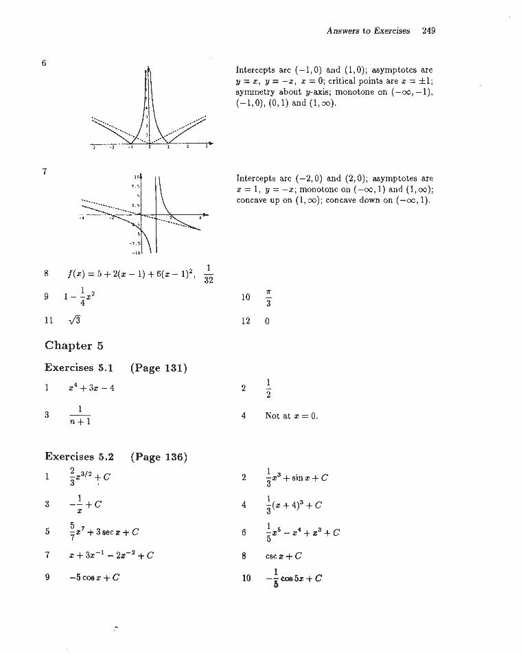
Answers to Exercises 249
Intercepts are (-1,O) and (1,O); asymptotes are y = x, y = -2, x = 0; critical points are x = f 1; symmetry about y-axis; monotone on (-00, -l), (-110)1 (0, 1) and (Loo).
Intercepts are (-2,O) and (2,O); asymptotes are x = 1 , y = -x; monotone on (-co, 1) and (1, co); concave up on (1, oo); concave down on (-oo, 1).
Chapter 5
Exercises 5.1 (Page 131)
1 x4+3x-4
Exercises 5.2 (Page 136)
4 Not at x = 0.

250 Answers to Exercises
Exercises 5.3 (Page 150)
1 L ( f , P n ) = $ l u ( f , P n ) = $
73249 26581 3 - L ( f l P n ) = m , U ( f t P n ) = m
5 A + C
7 A - B + C
9 F - E
Exercises 5.4 (Page 156)
Exercises 5.5 (Page 161) 2 n
1 - s i n ( T x ) + C n
2 L ( f Pn) = 51 u ( f , Pn) = 14
4 L ( f , P n ) = g l U ( f . P n ) = v
6 B - C
8 D - E + F
10 D - E
12 2 C + E - F
14 B - C + E

Answers to Exercises 251
Miscellaneous Exercises (Page 181) 1 1
1 x + ; + C 2 i (x2+4)3J2+C
Chapter 6
Exercises 6.1 (Page 168)
1 63 64
2 - 3

252 Answers to Exercises
Exercises 6.6 (Page 173) 128s 64n
1 - 7
2 - 15
Exercises 6.3 (Page 177) 1 1 - [133/2 - 53/21 1 3
2 -[8 * lo3/' - 133/2] 27
1 5 - 81
27
Miscellaneous Exercises (Page 178)
Chapter 7
Exercises 7.1

Answers to Exercises 253 .
cot x 11 -2 tan(2z + 3) 1
12 -- 1-2
1 z l n 1x1
14 cscxsecz
Defined for x > 0; monotone increasing for x > 0; concave down for z > 0.
Defined for x > 0; monotone decreasing for 0 < z < 1, increasing for x > 1; concave up for z > 0; relative minimum of 1 at x = 1. Defined for R - {O).- (1); monotone decreasing on (-00, O), (i, 1); monotone increasing on (0, i), ( 1 , ~ ) ; relative maximum of - ln4 at x = 4; concave down on ( - w , 0), ( 0 , l ) and (11.0). Defined for ( -2 , l ) U (1, w ) ; monotone increasing on (-2, -1) and (1 ,w) and monotone de- creasing on (-1, l ) ; concave down on (-2, I), ( 1 , ~ ) ; relative maximum of In4 at z = -1.
Exercises 7.2 (Page 190) 1 4e4" 2 -3e-3x

254 Answers to Exercises
(3 sin z + coa x)e3= 1
14 -(e" - e-=) 2
20 2(sin x + x cos x ) e2xsinx
Monotone decreasing on ( - m , -1); increasing on ( - 1 , m ) ; concave down on ( - m , -2); con- cave up on ( - 2 , m ) ; critical point x = -1; relative minimum at (-1, -e").
Monotone decreasing on ( - m , 2) ; increasing on (2 , m ) ; concave up on (-00, m ) ; critical point is x = 2; relative minimum at (2 , em4).
Monotone decreasing on (0 , e - I ) ; monotone increasing on (e" , m ) ; concave up on (0, m ) ; relative minimum of -e-I at x = e- I .
Exercises 7.3 (Page 196)
1 3"1n3

Answers to Exercises 255
Exercises 7.4 (Page 199)
1 4 x = ? , relative max. at (i, p + &)
16 t - tan-' x + C

256 Answers to Exercines
A 17 .-
2
Exercises 7.5 (Page 203) 1 xa - 1
5 2xcosh(x2) 6 - sinh(1n 1x1) = - X 2xa
1 x 13 - c o s h 4 x + c
4 14 arcsinh (-) + C
2
X 15 arccosh (-) + C 1
4 16 -arcshh (32) + C
3
17 12
18 i(arccosh 4 - arccosh 2) 2
Miscellaneous Exercises (Page 204) 1 -tanx 2 secx
10 x + tan-' x + C
Chapter 8
Exercises 8.2 (Page 211) .
1 2 lnI lnx l+C
x 9 sin-' - + C
3

Answers to Exercises 257
1 1 n 3 zain[(22 + I)'] + C 4 --
a n + l (ax + b);f+' + C
2 5 -(x - 1)312 + 2 ( ~ - 1)112 + c
3 6 z ( x - I) ' /~ + %(? - 1)312 + 2(x - 1)'12 + c
5
7 2d-+c 2 22 + 3
t a n - I - 8 - fi +c
3 4 x + 1 & x 2 + x - 3 9 -cash-' - + + C
3 + , / m - + C 8 5 2 f i 10 d a - 3 l n 1 2x 1
1 3 + w + C I1 - 1 n ) 3 2x 1 12 - s in3x - - s in6x+C 1 1
3 5
2 13 -- 10
15 14 -
3
4 15 -
15
Exercises 8.3 (Page 216) 1
1 - l n 1 x + l I + - l n ( x 2 + 1 ) + C 1 1 1 2 - - - - 1
2 3 2 - 1 9 In 12 + 11 + g ln 1x + 21 + C

Exercises 8.4 (Page 219) 1 1 1 1
1 - - c a 2 z - - c a 8 z + C 4 16 10 18
2 - s inSx+- s in9z+C
Exercises 8.5 (Page 224) 1 c o s x + x s i n x + C 2 -(x + 1)e" + C
3 2 c o s x - x 2 ~ o s x + 2 x s i n x + C 1 1
4 -- + - ( I + x2) tan-' x + C 2 2
1 1 13 --x cos(1n x) + - sin(1n x) + C
2 14 -22 + 2 tan" x + x ln(1 + x2) + C
2 .

Answers to Exercises 259
Exercises 8.6 (Page 231)
11 ~ x n c ~ x d x = x n s i n x + n x n - ' c o a x - n ( n - 1) / zn-2 cos x dx and thus
1 n n(n - 1) xn sin a x dx = - - x n cos a x + -xn-' sin a z - - znn-a sin a z d x and thus
a a2 a2 1 3 3 1 x 4 s i n 2 x d x = --x4cos2x-x3sin2x+-x2tos2x- - x s i n 2 x - - c o s 2 x + C 2 2 2 4
n- d x = Axn-' J= - - dx and thus n
MisceManeous Exercises (Page 232)

260 Answers to Exercises
2 8 8 5 -(z - 2)'Ia + -(z - 2)6/a + 5(z - 2)=Ia + c
7 5
6 2 f i + 6 l n I f i - 3 1 + C 7
1 1 22 + 3 8 -secz - c o s x + C
2 Jii tan-' - 9 - ln1x2+3x+51- - Jii
1 10 ?(z2 + z + 1)3/2 + :(2x + l)&FZT+ ln(z + + + c
11 12 sinh-' x + C or ln(x + Js) + C 9 x
1 2 13 -2 tan-' x + - ln(x2 + 1) + C 14 2 1 n ( l + \ / 2 + - ) + l + J m + C
2
1 x 12 7 7 22 tan-' x + -In 1x - 21 - -In 1x + 21 + C 5 x 2 + l 25 100 100
23 (x2 - 22 + 2)e" + C 1
24 - - c o t 2 z - l n I s i n x l + C 2

Greek Alphabet 261
Greek Alphabet
Greek letter
a A
B B
Y r 6 A
E E
C tl H
8 0 t?
I 1
K K
A A
D M
Name
Alpha
Beta
Gamma
Delta
Epsilon
Zeta
Eta
Theta
Iota
Kappa
Lambda
Mu
Greek letter
v N
s 0 0
K n P p
a Z
T T
v Y
$' Q
X x W Y
o a
Name
Nu
Xi
Omicron
Pi
Rho
Sigma
Tau
Upsilon
Phi
Chi
Psi
Omega
Some Mathematical Symbols
I I absolute value, modulus 1 n intersection
D-' antiderivative
X Cartesiah product
( ) combination, of n objects talring
r at a time d
D , - derivative with respect to x dr
f-' inverse of a function f
E membership
max maximum (of)
Q n th root of
Z set of integers
dom domain
0 empty set
I, dr iotegral with respect to x
n ! n factorial
f : A * B f a function from A to B
N set of natural numbers
R- set of negative real numbers
z+ set of positive integers
R+ set of positive real numbers
R set or real numbers
A&B fafunctionfromAtoB summation
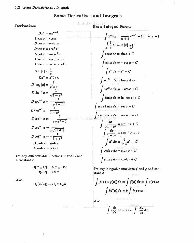
262 Some Derivatives and integrals
Derivat ivee
Some Derivatives and Integrals
Oxn = n ~ " - ~
Deinz = cosx Dcoax = -sin%
Dat = at In a
1 P log, 1% 1 = - z lna
D sin-' z = 1
J1 -22
1 D tan" x = -
1 -txa
D csc" z = 1
-m
D cosh x = sinh z Dsinhx = coshx
For any differentiable functions F and G and a constant k
Basic Integral Forme
J cwzdx = s h x + C
J sinxdz = -cosx + C
J e z d z = e i + ~
Jmc'zdz = t a n z + ~
J csc2xdx = - c o t z + C
J tanxdz = lnIsecx(+C
J s e c x t a n t d z = s e c z + C
cscxcotzdx = - c s c x + C
J coahxdx = s i n h z + C
J sinhxdx = coshx + C
For any integrable functions f and g and con- stant k
Also

Index 263
Index
absolute value function, 5 acceleration, 88 affine function, 7 antiderivative, 129
definition, 130 antidifferentiation, 129 approximation
cubic, 120 linear, 119
arbitrary constant, 131 arc length, 174 area, 137, 163
element of, 164 asymptote, 111
horizontal, 111 oblique, 112 vertical, 112
average velocity, 51 chain rule, 69 characteristic function, 2 codomain, 1 '
concave, 100 down, 100 up, 100
concavity, 100 constant function, 3 constant of integration, 154 continuity, 41
at a point, 41 on an interval, 43 polynomials, 45 theorems on, 45 trigonometric functions, 46
coordinate, 1 critical point, 98 curve
length of, 174 curve sketching, 114 definite integral. 142 derivative, 52
definition, 52 first, 52 higher order, 78
left-handed, 55 power function, 56 product, 63 quotient, 65 right-handed, 55 second, 78 sum, 60 trigonometric functions, 58
differentiable, 53 at a point, 53 in an interval, 53
differential coefficient, 52 differential, 121 differentiation, 53
implicit, 72 logarithmic, 193 rules of, 60
disc method, 168 discontinuity, 41
essential, 44 jump, 44 removable, 43 types of, 43
domain understood, 14
error, 117 exponential
function, 186 natural, 186 to other base, 191
extrema (see maximum or minimum) Fermat's principle, 108 first derivative test, 99 function, 1
absolute value, 5 affine, 7 approximation of, 117 characteristic, 1 composite, 10 composition of, 10 constant, 3 continuous, 41 ,
decreasing, 95
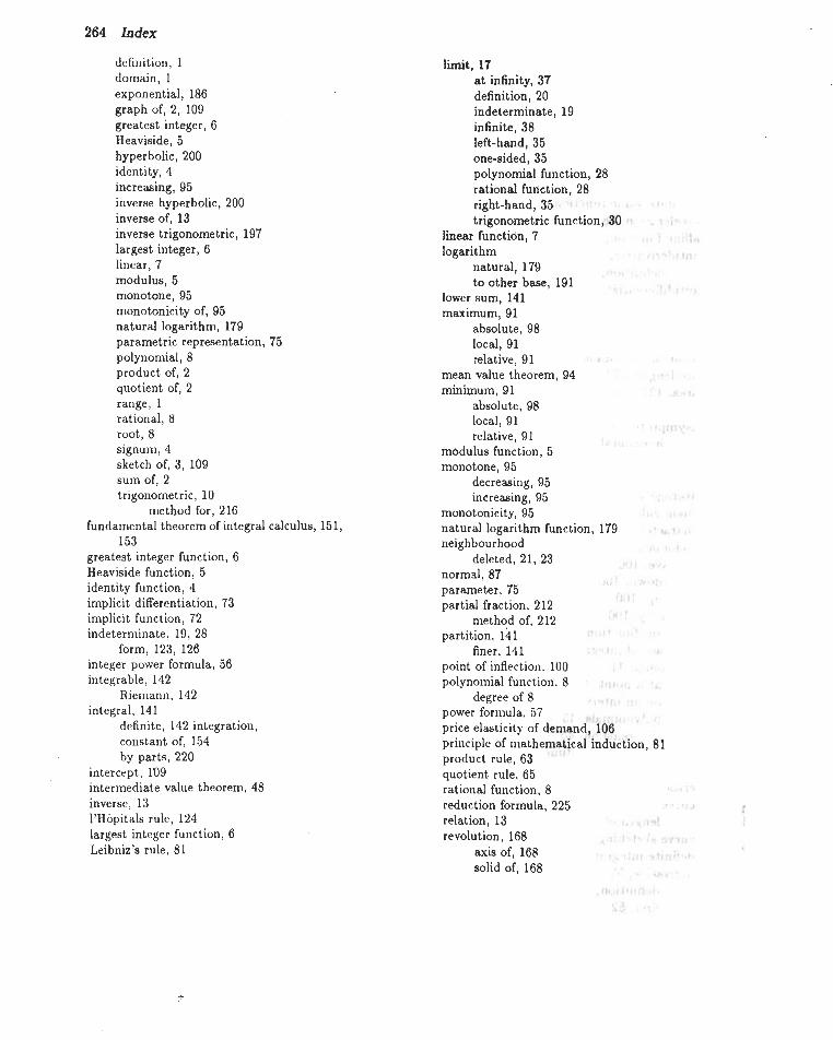
definition, 1 domain, 1 exponential, 186 graph of, 2, 109 greatest integer, 6 Heaviside, 5 hyperbolic, 200 identity, 4 increasing, 95 inverse hyperbolic, 200 inverse of, 13 inverse trigonometric, 197 largest integer, 6 linear, 7 modulus, 5 monotone, 95 monotonicity of, 95 natural logarithm, 179 parametric representation, 75 polynomial, 8 product of, 2 quotient of, 2 range, 1 rational, 8 root, 8 signum, 4 sketch of, 3, 109 sum of, 2 trigonometric, 10
method for, 216 fundamental theorem of integral calculus, 151,
153 greatest integer function, 6 Heaviside function, 5 identity function, 4 implicit differentiation, 73 implicit function, 72 indeterminate, 19, 28
form, 123, 126 integer power formula, 56 integrable, 142
Riemann, 142 integral, 141
definite, 142 integration, constant of, 154 by parts, 220
intercept, 109 intermediate value theorem, 48 inverse, 13 I'Hopitals rule, 124 largest integer function, 6 Leibniz's rule, 81
limit, 17 at infinity, 37 definition, 20 indeterminate, 19 infinite, 38 left-hand, 35 one-sided, 35 polynomial function, 28 rational furiction, 28 right-hand, 35 trigonometric function, 30
linear function, 7 logarithm
natural, 179 to other base, 191
lower sum, 141 maximum, 91
absolute, 98 local, 91 relative, 91
mean value theorem, 94 minimum, 91
absolute, 98 local, 91 relative, 91
modulus function, 5 monotone, 95
decreasing, 95 increasing, 95
monotonicity, 95 natural logarithm function, 179 neighbourhood
deleted, 21, 23 normal, 87 parameter, 75 partial fraction, 212
method of, 212 partition, 141
finer, 141 point of inflection, 100 polynolnial function. 8
degree of 8 power formula, 57 price elasticity of demand, 106 principle of mathematical induction, 81 product rule, 63 quotient rule, 65 rational function, 8 reduction formula, 225 relation, 13 revolution, 168
axis of, 168 solid of, 168

Index 266
Riemann integrable, 142 Riemann sum, 164 Rolle's theorem, 93 root function, 8 sandwich theorem, 30 second derivative test, 101 shell method, 168, 172 signum function, 4 singular point, 53 sketch of a set, 2 slice method, 168 Snell's law, 108 source set, 1 standard integrand, 205 stationary point, 91' substitution
circular, 208 hyperbolic, 208 method of, 157, 206 trigonometric, 208
symmetry; 109 tangent, 86 target set, 1 Taylor's formula, 120 Taylor's theorem, 120 Taylor's approximation, 120 triangle inequality, 6 upper sum, 141 variable, 1 volume, 168
solid of revolution, 168 washer, 169
