university of illinois at chicago bioengineering student journal
TRANSCRIPT


UBSJ
University of
Illinois at
Chicago
Bioengineering
Student Journal
Spring 2016
Vol. VII No. 1
CHIEF EDITOR Cierra Hall
EDITORS
Brynne Nicolsen
Christine Joseph
REVIEWERS
Ken Blank
Jesse Gerringer
Tooba Ghafoor
Mark Hillstrom
Jagan Jimmy
Maziyar Khansari
Rebecca Mitra
Gregory Roytman
Abhinav Subramaniam
Xinge Wang
COVER ARTISTS Christine Cote
Michelle Lamont
FACULTY ADVISOR
Professor Richard Magin
Contact: [email protected]
Phone: (312) 996 – 2335 fax: (312) 996 - 5921
UIC Bioengineering Student Journal
Richard and Loan Hill Department of Bioengineering,
University of Illinois at Chicago, Science & Engineering Offices
(SEO), Room 218 (M/C 063)
UBSJ IS A UNIVERSITY OF ILLINOIS AT CHICAGO BIOENGINEERING
STUDENT PUBLICATION

UIC Bioengineering Student Journal
Spring 2016
Vol. VII No.1
Contents
Foreword
i
CARBON NANOTUBES AS A MEDICAL IMAGING TOOL
Jessica Cleary
1
THE DISCOVERY OF RADIOACTIVE ELEMENTS THAT LED TO
BIOMEDICAL ADVANCEMENTS
Lauren Curie
6
EEG ARM WRESTLING
Samuel Dryer and James Steele
13
EXTRACORPEAL SHOCK WAVE THERAPY
Mark Hillstrom
16
IMAGING TECHNIQUES IN THYROID SCANNING
Niketha Kailash
21
NUMERICAL ANALYSIS OF THE RELATIONSHIP BETWEEN CROSS-
SECTIONAL AREA AND PRESSURE IN OVINE AORTA USING THE
KELVIN VISCOELASTIC MODEL
Gregory Roytman
27
SUPERIORITY OF PROTON CT AS AN ALTERNATIVE TO X-RAY CT
FOR USE IN PROTON THERAPY TREATMENT PLANNING
James Steele
33
MODELING THE EFFECTS OF TEMPERATURE CHANGES ON
CARDIAC PURKINJE FIBERS
Martin Strama
38
BIOPSYCHOSOCIAL VARIABLES AND THE EFFECTS ON IMMUNE
SYSTEM: AN ANALYSIS OF THE RELATIONSHIP BETWEEN
NEGATIVE MOOD STATES AND PRO-INFLAMMATORY CYTOKINES
Nneka Ukegbu
44

Foreward
This year I am happy to present the seventh volume of the UIC Bioengineering Student Journal. Over
the five years that I have been involved with the journal as a reviewer, editor, and during this second time
that I am serving as Editor-In-Chief, I have had the pleasure of meeting and working with many talented
bioengineering students. It is my hope that in the course of writing and reviewing articles, and by serving
on the editorial board, students experience academic and personal enrichment in the bioengineering
department here at UIC. Undergraduate students that strive to succeed not only in their coursework, but
also in extracurricular activities such as the UBSJ and research, graduate with not only a superior resume,
but with a more finely honed set of personal and academic skills.
Although I am finally reaching the end of a ten year period of study at UIC (B.S. 2011, Ph.D. 2016), my
experiences will be fondly remembered, along with the UIC students and faculty that I worked with,
through UBSJ and otherwise. The students that will continue to facilitate our journal will have many
wonderful journal issues to look back on for reference and inspiration, and I am sure that each new issue
will continue to be better than the last.
I would like to thank our Faculty Advisor, Dr. Magin, for giving us all the freedom and opportunity to
create a truly student-led project and for allowing us to bring our visions to life. I would also like to thank
Department Head Dr. Royston for continually supporting the journal’s financial and logistical needs and
allowing us to host release parties every year. Lastly, I would like to thank and congratulate the authors,
reviewers, and editors who worked tirelessly to make this year's issue of the journal such a great success.
Cierra Hall
Editor-In-Chief

1
Carbon Nanotubes as a Medical Imaging Tool Jessica Cleary
Abstract Early detection and non-invasive disease monitoring are crucial parts of disease treatment. The
difficulties with these aspects are largely due to the limitations of current imaging techniques. A
potential solution to these constraints could lie within one of the most common elements in
biological systems, carbon. The valency of carbon allows it to form many different allotropes. These
include a variety of shapes and commonly known forms such as diamond and graphite as well as
more unusual forms like fullerenes. One of these atypical forms, carbon nanotubes, has recently
become a common topic of research. The popularity of research into carbon nanotubes (CNTs) is
due to their superior physical properties which confer many potential applications in medicine and
industry. The extraordinary strength, elasticity, conductivity, and optical properties of CNTs have
been well documented. They are of particular interest to the field of medical imaging because their
application could provide low-risk and high resolution imaging of live cells. Some interesting
applications include CNTs based detectors that can detect terahertz frequency waves, injection of
fluorescent CNTs with subsequent imaging, and CNTs based magnetic resonance imaging (MRI)
contrast agents. These and many other applications are limited by factors such as the degree of
toxicity of CNTs in biological systems and manufacturing complications. Current research is based
on navigating challenges involved with CNT applications, and could potentially lead to highly
efficient and effective methods for widespread utilization of CNTs.
Keywords: Carbon Nanotubes, allotropes, Medical imaging
1. Introduction
The existence of carbon nanotubes was proposed
theoretically in 1990 by Rick Smalley based on his
research with buckminsterfullerene. He found the
mysterious compound when he was testing
abnormalities in the mass spectrometry of graphene.
[9]. Although CNTs were probably observed
experimentally many years before this, the importance
of fullerenes was just coming to light, thus providing
the motivation to delve deeper. Shortly after Smalley's
proposal, transmission electron micrographs provided
physical evidence of existence of CNTs. Ever since
that time CNTs have become widely popular among
researchers. An example of CNT imaged by
transmission electron micrograph is shown in figure 1.
The study of carbon nanotubes is an important venture.
CNT application opens enormous possibilities in a
wide variety of industrial and medical applications. It
is particularly significant for medical imaging because
of the scope and variety of potential applications.
Previous impractical and inefficient methods could be
brought within the realm of routine practices. With
careful analysis and development, these tiny
molecules can be used as detectors, emitters, and
contrast agents. All of these instruments already exist
in imaging. Therefore, intensive study of CNTs begs
the question of their superiority over current agents.
CNTs must have some advantage and enough so that
companies and government grants will fund their
research.
This indeed turns out to be the case. CNTs display
unique physical properties which yield many
advantages over current instruments. In this article the
focus is on application of CNTs in medical imaging.
Pending applications and challenges are discussed.
2. Carbon Nanotube Structure and
Properties
Figure 1. Electron Micrograph of a SWNT [3]

2
2.1 Carbon Bonding and Structure
Carbon nanotubes are made of a crystalline network
of sp2 hybridized carbon atoms. This network forms a
tubular scaffold which can exist in single or multiple
walled forms [8]. The physical strength of CNTs are
due to the strength of Carbon bonding. The sp2 bond
is 33% stronger than the sp3 bond of diamond, the
hardest known mineral [13].
Furthermore, carbon nanotubes have extremely high
surface area due to the fact that all their atoms are on
the surface (see figure 2).. This property make them
very useful for biomedical applications. Many
different molecules can be conjugated to CNTs so they
can be conjugated in ways that target particular cells
and biomolecules. For example, they can be attached
to antibodies or cell recognition proteins. This
property is a major value of CNTs in medical imaging.
Surface conjugation makes CNTs particularly useful
tool which can provide functional physiological
information and can be beneficial in structural imaging
[8].
2.2 Single and Multiple-Walled Carbon
Nanotubes
The more studied and more currently useful form of
CNTs are single-walled carbon nanotubes (SWNT).
They are made up of a single sheet of graphene rolled
into a tubular shape (Figure 2). These are essentially
one atom thick and usually do not necessarily have a
constant radius. They can exist as different sizes in
diameter and length, ranging from 0.4 – 4 nm in
diameter and from 50 nm up to 1cm in length [16].
Figure 2. Structure of a single-walled carbon nanotube
(SWNT) [3]
Multiple-walled carbon nanotubes (MWNTs) are
simply concentrically stacked SWNTs. They can
consist of many different layers of graphene. While
they don't exhibit the same optical properties of
SWNTs, their larger size may provide an adequate
platform for conjugation with larger biomolecules [6].
2.3 Properties
2.3.1 Electrical and Thermal Conductivity
Depending upon the strength of a magnetic field
applied to CNTs, they can be induced to be either
semi-conducting or metallic [8]. A very small
magnetic field applied parallel to the tube axis make
them semiconductors. Conversely, when a high
magnetic field is applied, they become metallic. This
unique phenomenon is due to a gap in energy band.
This property is particularly of interest to scientists
who are working on terahertz frequency detectors [4].
In addition to electrical conductivity, CNTs have very
high thermal conductivity. They remain stable up until
temperatures nearing 4000K [13]. This varies however
with the size of the nanotubes. Like most of their
properties, their thermal and electrical conductivity are
only as reliable as the preciseness of their synthesis.
2.3.2 Strength and Elasticity
CNTs also exhibit strength and elasticity which far
outcompete other materials. Their strength is due to
the carbon bonding and elasticity is a function of their
size. There are different possibilities for the interlayer
spacing, which in turn are responsible for the degree
of elasticity. It is easy to imagine that a SWNT with a
large radius would be more elastic than one with a
smaller radius as the angle of carbon bonding in a
tighter circle is more strained.
Perhaps the illustration of a Chinese finger trap
demonstrates this. As the diameter decreases (trapping
fingers in the process), the rigidity of the trap
noticeably increases [13]. Nevertheless, even CNTs
with relatively small radii exhibit elasticity that far
surpasses other materials. Nanotubes of varying
diameters have shown the highest ever measured
Young's modulus (standard measure of elasticity)
[13]. This elasticity could facilitate bending of the
CNTs to allow multiple binding sites of functional
groups which would lead to enhanced binding affinity
of nanotubes [6].
2.3.3 Optical Properties
SWNTs have sharp densities of electronic states which
imparts distinct optical properties. Semiconducting
SWNTs have small energy band gaps, thus exhibit
photoluminescence in the near-infrared (NIR) range
[6]. They also have distinctive resonance-enhanced
Raman signatures for Raman detection and imaging.

3
3. Imaging Application
The properties of CNTs make them useful in many
different imaging modalities. A few examples of
applications still in process are highlighted in Table 1.
As these areas of CNT use are explored, more potential
applications could surely be pictured.
Table 1. CNT applications
Properties Application Advantage
Semiconductance Terahertz
Detectors
Development
of Terahertz
technology
High Surface Area MRI
contrast
agent
Enhanced
relaxivity
Photoluminescence Near
Infrared and
Raman
Imaging
High
resolution
and
physiological
information
3.1 CNT Detectors
Studies of CNTs have shown extensive detection of
electromagnetic radiation at many different
frequencies. This property has led to the investigation
of the extent of their limitations in this area. Unlike
other imaging detectors, those made from CNTs could
detect frequencies up to the terahertz wavelength [15].
The benefit of terahertz detection is that it is safe, non-
invasive, and painless. These extremely high
frequency waves are non-ionizing and their low
photonic energies do not damage tissues and DNA.
They can also penetrate a wide variety of materials,
including the human body. The difficulty with
terahertz waves is that there are limited number of
materials that can absorb that frequency of photonic
wavelength and convert it into an electrical signal.
This problem could be solved by use of carbon
nanotubes [17]. In fact, SWNTs have been used to
create a thin film of nanotubes which detect the high
frequency waves. Development of viable terahertz
detectors have been in progress for years, and CNTs
just may be the highly sought-after answer [15].
3.2 CNT Fluorescence
We have discussed that SWNT surfaces can be
modified to target certain cells. This becomes
particularly useful for near-infrared spectroscopy
(NIR) and photoacoustic imaging (figure 3). When
excited by shorter wavelengths (550-850nm), CNTs
emit frequencies in the NIR range (900-1600nm). This
is a phenomenon known as Raman scattering. The
large difference between incident and scattered
wavelengths reduces background from Raman
scattering of tissues and is the basis of fluorescence in
the NIR range [8].
Figure 3. Surface conjugation and photoluminescent tumor
targeting [6]
NIR light is normally harmless to the body and can
penetrate tissues which are intrinsically non-
fluorescent. This would allow contrast between
normal tissues and those targeted by CNTs. This has
already been used as a way to image endocytosis and
exocytosis of SWNTs in biological cells in real time
[16]. SWNT targeting of cancer cells can also enhance
tumor recognition. For example, SWNTs have been
functionalized with folate which has many receptors
on cancer cells. The cancer cells then allow
functionalized SWNTs to enter while normal tissues
without folate receptors remain free of SWNTs. Thus,
SWNTs are localized to cancer cells and can be
detected with NIR or even destroyed by NIR laser
radiation [8].
The photoluminescent properties of SWNTs can also
be used in photoacoustic imaging. Photoacoustic
images are superior to ultrasound because they have
high resolution and allow deeper penetration than NIR
imaging. This is yet another way in which CNTs could
enhance development of an imaging modality that is
new and superior to commonly used methods. The
cellular recognition tripeptide RGD can be attached to
SWNTs and used to target certain tissues and create
contrast in photoacoustic images (Figure 3) [6].

4
SWNTs can also be used in Raman microscopy to
image cells. They have distinctively strong resonance
Raman scattering because of their quasi 1-D nature.
Their electron density states cause strong isotopic
peaks which can be easily distinguished from other
tissues. To fully realize their potential in Raman
imaging, isotopically unique SWNTs can be
conjugated with various targeting ligands. This
effectively color codes images because different
isotopes produce different Raman shifts [6]. These
methods for innovative manipulation of CNT optical
properties are intriguing and further exploration of
these ideas could produce completely new imaging
styles.
3.3 MRI Contrast Agents
Since magnetic resonance imaging (MRI) is a safe and
highly effective method of medical imaging, much
effort is put into advances in its utilization. The ability
to image soft tissue with high resolution and without
use of ionizing radiation is unique to MRI. It can also
provide functional information, much like positron
emission tomography (PET) imaging, but with sub-
millimeter resolution. This information requires the
use of a contrast agent which can not only be targeted
to specific biomolecules but also produce a signal
strong enough to be detected.
CNTs could hold potential value as a contrast agent,
and research to develop this technology is under way.
Nuclear magnetic resonance (NMR) produces images
in MRI by detecting variations in proton density via
magnetic spins, and for this reason a pure carbon
compound like a CNT cannot be detected. Since CNTs
do not have any protons available for detection they
must be altered to produce a form that is useful to MRI
[11]. Researchers have found that the hollow tube
structure can be used to trap magnetic particles which
produce a signal that can be detected by NMR. Surface
functionalization or conjugation of CNTs can also
alter their chemical makeup to render them useful in
NMR.
Contrast arises from differences in signal arising from
water content of tissue. The differences in water
content are indicated by different tissue relaxation
times of hydrogen nuclei termed T1 and T2 [14]. The
proton density of the tissue, (x,y), in addition to these
relaxation times are proportional to (denoted by ) the
intensity of the signal, I(x,y). The relationship
between the intensity of signal and T1 and T2 times is
given by:
𝐼(𝑥, 𝑦) ∝ 𝜌(𝑥, 𝑦)(1 − 𝑒−𝑇𝑅
𝑇1)𝑒−𝑇𝐸
𝑇2 (1)
Strong signals can be detected from separate tissues
but unless their relaxation times differ they cannot be
distinguished. This is where contrast agents come into
play. These agents shorten relaxation times in target
tissues by exerting a magnetic force upon the
surrounding water protons. Paramagnetic complexes
such as Gadolinium and Manganese chelates
accelerate T1 relaxation and Superparamagnetic
nanoparticles like iron oxide accelerate T2 relaxation.
The resulting signal with addition of contrast is given
by the equation:
[𝑇𝑖]−1 = [𝑇𝑖
0]−1
+ 𝑟𝑖[𝐶𝐴] i = 1,2 [11] (2)
Where ri is the relaxivity of the agent (a measure of the
change in relaxation implemented by the contrast).
[CA] is the concentration of the contrast agent and Ti0
is the relaxation time without contrast. This equation
illustrates that the signal intensity for MRI depends not
only the concentration of the agent but also its
relaxivity. Currently used contrast agents require
relatively high concentrations in order to produce
desired effect [12]. This must be monitored carefully
since those agents can be toxic in high concentrations.
A contrast agent with higher relaxivity than existing
agents would require a lower concentration to achieve
the same effectiveness. This scenario is clearly
desirable because minimizing injection of potentially
toxic materials reduces risk to the patient. It turns out
that SWNTs conjugated with magnetic particles can
yield enhanced relaxivity. For example, Gadolinium-
loaded CNTs exhibit an effectiveness that is 40-90
times larger than any present contrast agents [11].
Other CNT-linked substrates such as NMR active
isotopes like 19F are under scrutiny for use as contrast
agents. These are still in developmental phases since
they are still insoluble and toxic [11].
4. Current Research
In order for Carbon Nanotube use to have a significant
impact, development of standardization and quality
control must be achieved. Many potential applications
are limited by the unpredictability inherent of the
manufacturing process. It is difficult to control the
purity of a CNT sample (such as creating only SWNT
instead of a mixture with MWNT) and much of current
research is based on quality control [8].
Further investigation of their properties could yield
many exciting discoveries, but perhaps the focus right
now should be on the manufacturing process. Owing

5
to their extremely small size (figure 1), it can be
difficult to control the exact length and radius of each
tube and any defects could potentially render them
toxic in a biological environment. There are many
different methods of CNT synthesis and this should be
the focus of research [13].
All forms of manufacturing involve very high
temperatures which presents a physical challenge.
Different methods produce varying results, and there
are costs and benefits and to all of these processes. A
close analysis of the tradeoffs involved could reveal
the superiority of some methods over others [13].
Whatever the chosen process, synthesis and use of
CNTs is sure to be an exciting field of discovery with
the next few decades.
5. References
1. Gong, H, Z. Liu, and R. Peng. Carbon nanotubes
for biomedical imaging: the recent advances. Adv.
Drug Deliv Rev. 65(15): 1951-63, 2013
2. Carbon Allotropes. Reference: SWNT-001
[accessed 2015, Oct 16].
http://www.carbonallotropes.com/carbon-
nanotubes/39-single-wall-carbon-
nanotubes.html.
3. Nanocomp Technologies, Inc. Solutions: What
are Carbon Nanotubes. c 2014 [accessed 2015,
Oct 16]. http://www.nanocomptech.com/what-
are-carbon-nanotubes.
4. Janes, Mike. 2014, June 13. Sandia Labs News
Release. [accessed 2015, Oct 17].
http://www.sandia.gov/news/publications/
labnews/archive/14-13-06.html.
5. Bagley A. F., A. M. Belcher, S. N. Bhatia, M. J.
Birrer, and Ghosh, D.. Deep, noninvasive imaging
and surgical guidance of sub-millimeter tumors
using targeted M13-stabilized single-walled
carbon nanotubes. PNAS 111:13948-13953, 2014
6. Dai, H., Z. Liu, S. Tabakman, and K. Welsher.
Carbon Nanotubes in Biology and Medicine: In
vitro and in vivo Detection, Imaging and Drug
Delivery. Nano Res. Springer 2:85-120, 2009
7. Holland, J. P., J. Lewis, C. May, M. R. McDevitt,
S. Ruggiero, D.A. Scheinberg, S.R. Sprinkle, and
C. Villa. Imaging and treating tumor vasculature
with targeted radiolabeled carbon nanotubes. Int.
J Nanomedicine. NCBI 5:783-802, 2010
8. O'Connell, M. J. Carbon Nanotubes: Properties
and Applications. CRC Press, Taylor and Francis
Group. 2006
9. Smalley, R. E. Formation and properties of C60
and the fullerenes. National Institute of Standards
and Technology 1990
10. Material Scientist Talk. CC-BY-SA-3.0;
Released under the GNU Free Documentation
License. June 4 2009
11. Anuganti, V., and A. Velders. Nuclear Magnetic
Resonance Spectroscopy and Imaging of Carbon
Nanotubes. Supramol. Chemistry and
Technology. Feb 2011, Chapter from Carbon
Nanotubes for Medical Application pp.125-150.
12. Lu, Z., Z. Zhou. Gadolinium-Based Contrast
Agents for MR Cancer Imaging. Wiley
Interdiscip. Rev. Nanomed. Nanobiotechnology.
5(1): 1-18, 2013
13. Dresselhaus, G., Dresselhaus, M., Jorio, Ado.
Carbon Nanotubes: Advanced Topics in the
Synthesis, Structure, Properties and Applications.
PACS, Springer 2008
14. Smith, N.B., A. Webb. Introduction to Medical
Imaging: Physics, Engineering, and Clinical
Applications. Cambridge University Press 2011
15. Adams, S., C. Chan, K. Fu, J. Nicholson, E. Plizzi,
S. Yngvesson, and R. Zannoni. Terahertz deection
in single wall carbon nanotubes. Department of
Electrical and Computer Engineering, University
of Massachusetts 2007
16. Liao, H., B. Paratala, B. Sitharaman, and Y.
Wang. Applications of Carbon Nanotubes in
Biomedical Studies. Sarah J. Hurst (ed.),
Biomedical Nanotechnology: Methods and
Protocols, Methods in Molecular Biology, vol.
726 Springer, 2011
17. Kibis, O.V., M.E. Portnoi, and M. Rosenau da
Costa. Carbon Nanotubes as a basis for terahertz
emitters and detectors. Microelectronics Journal,
European Nano Systems 40(4–5): 776-778. 2009

6
THE DISCOVERY OF RADIOACTIVE ELEMENTS THAT LED TO
BIOMEDICAL ADVANCEMENTS Lauren Curie
Abstract Wilhelm Roentgen was the first to discover the existence of X-rays. He discovered that rays could
travel through solid objects, and not knowing much about the science behind this new
phenomenon, he labeled them X-rays, X standing for unknown. Shortly after this discovery, Henri
Becquerel witnessed a similar occurrence with uranium, which peaked Marie Curie’s interest, and
eventually led to her finding of radium and polonium. From studying Becquerel and Roentgen’s
findings further, yet another discovery was made, this time by Paul Villard and Ernest Rutherford.
Together they uncovered another type of ray that Rutherford labeled as a “gamma ray.” The
science behind these discoveries was indeed groundbreaking and soon after, radioactive spas
started emerging around the globe and cures to many ailments were believed to be from these
newfound radioactive elements. While we know now that radioactive elements must be handled
with extreme care, a great deal of good has come from these discoveries. X-ray and nuclear
imaging techniques are still used today and are based off of the science from these experiments.
Delving into these discoveries further, we can see how these scientists have helped the world of
biomedical imaging, and society as a whole.
Keywords: Biomedical Imaging, X-ray, PET, SPECT, CT, radioactivity
1. Introduction
A series of events led to the discovery of radioactive
material. In December of 1895, a man by the name of
Wilhelm Roentgen discovered that rays could travel
through solid objects, not knowing much about these
rays, he labeled them as X-rays, X standing for
unknown. His research began at the University of
Wurzburg, where he focused on light phenomena by
discharging electrical current in Crookes tubes. In
1901 he was awarded the first Nobel Prize in physics
for his finding of a “different type of ray” [1].
Shortly after his discovery, Henri Becquerel
discovered a similar phenomenon with uranium.
Becquerel’s discovery happened by accident, when
he put his uranium salts and photographic plates in a
drawer on a cloudy day. He found that the images of
the crystals were outlined on the plates, even though
they had not been in direct sunlight. The results were
astounding to Becquerel; however most ignored this
finding because it seemed too similar to Roentgen’s
discovery. The mystery associated with Becquerel’s
work lured Marie Curie into learning more about
uranium. Since there was very little literature on this
subject at the time, she went straight away to the lab
to run experiments. It was while Marie was working
with pitchblende, which is a form of the mineral
uraninite occurring in brown or black viscous masses,
that she noticed a highly radioactive substance that
was greater than uranium [2]. Her husband, Pierre
Curie, helped her and eventually they discovered two
new elements: radium and polonium. Industrial firms
saw this as a promising field of work and offered to
help the Curies by providing additional lab space. As
they gained more and more attention, they were able
to get the tools they needed to make further
discoveries in this realm of work, which eventually
led to some of the tools we have today in biomedical
imaging.
Figure 1. Image of pitchblende [3]
Five years after the discovery of X-rays came the
discovery of gamma-rays. In 1900, Paul Villard made
this discovery while investigating radiation form
radium [4]. Villard was running experiments on
radium and noted rays differing in penetrating depths,
but did not label this type of ray as separate from
alpha and beta rays, which had already been
discovered and labeled as a form of radioactive
decay. It wasn’t until a year later in 1901 that Ernest

7
Rutherford discovered in a separate experiment that
these types of rays that were emitting from uranium
were indeed different than alpha and beta rays; hence
he named them gamma rays [5].
2. X-rays Versus Gamma Rays
The difference between X-rays and gamma rays
stems from their origin and energy levels.
Figure 2. Spectrum comparing X-rays and gamma rays [6]
X-rays are produced by their change in energy states
of orbital electrons or by the deceleration of an
electron beam [7]. Gamma rays come from nuclear
decay and have much higher energies ranging from
80 to 200 keV, however gamma radiation within the
energies of 90 to 200 keV are better suited for camera
imaging and provide a source of activity that is short
lived, which lowers a patient’s radiation dose. It
should be noted that there are other types of nuclear
decay, such as alpha and beta rays, however gamma
rays have higher energies and are thus able to
penetrate sources better, making it a more suitable
option for imaging. X-rays have energy levels
ranging from a maximum energy of 150 keV and a
minimum energy of 20 keV [7]. The energy of an X-
ray or gamma ray can be calculated by the following
equation:
E = hc/ (1)
Where h is Planck’s constant and c is referencing the
speed of light. The wavelengths for X-rays vary
between 0.062 and 0.0082 nanometers. To better
illustrate where these wavelengths stand in a
spectrum as noted in Figure 2, visible light has a
range of wavelengths from 400 to 700 nanometers.
Gamma rays have wavelengths shorter than .001
nanometers. In general, a decreasing wavelength will
produce an increase in energy, based on the inverse
relationship seen in equation (1). Since gamma rays
characteristically have shorter wavelengths and
higher energies, they are assumed to be more
damaging based on this principle. Both ray types
pose a health risk due to ionizing radiation. This is an
undesirable property because it can lead to mutation
of cells in vivo, causing unwanted DNA, cells or
tissue damage. Alternatively, scientists were able to
find a use for this property by targeting unwanted
cells. X-rays and gamma rays can be used in
sterilization procedures to kill unwanted bacteria, or
in treatments to kill cancerous cells. Ironically, for
the very reason that they are dangerous, they can also
be used productively . X-rays and gamma rays differ
vastly in the ways in which they are produced, and
vary slightly in terms of their physical properties, but
ultimately the reasons that they are used in
biomedical imaging are for the same purpose.
3. X-rays and Computerized Tomography
Imaging
As Roentgen later figured out, in order for X-ray
production to occur, there must first be a source of
negatively charged electrons, or a cathode, which is
generally composed of tungsten. Energy is involved
when heat is present. Once the wire reaches around
2200 degrees Celsius the amount of energy in the
system will be sufficient to allow the electrons to
leave the cathode. Cooling systems are often present
to allow for proper heat removal. On the other end,
there is an anode, which is created by a large positive
voltage on a metal target. Once a voltage is applied,
electrons will leave the cathode and strike the anode.
A high-energy electron from the cathode ejects an
electron in the inner shell of the anode, causing an
outer electron to fill the hole. The resulting difference
in binding energies creates X-rays that are emitted.
Often a negatively charged focusing cup surrounds
the cathode to concentrate the electrons.
Figure 3. Image of X-ray emission [8]
Once these X-rays pass through the body, they are
either absorbed by bone or other tissue, in which case
they are attenuated, or they continue to travel towards

8
the detector to be picked up [9]. Two types of
detectors exist: computed radiography and digital
radiography. Computed radiography is composed of
phosphor crystals. When X-rays hit the phosphor
layer, electrons are released, eventually creating light.
This light leads to a latent image, which is ultimately
processed in a computed radiography reader.
Photodiodes convert light into voltage, which is then
filtered and digitized. The whole process can happen
in a mater of seconds. In the case of digital
radiography, there are two main types: indirect and
direct. Indirect digital radiography X-rays are first
converted into light by a scintillator before being
converted into a voltage. Direct digital radiography
eliminates the middle step.
Figure 4. Image of X-ray [10]
As you can see in Figure 4, bone appears brighter on
the X-ray image due to an increase in intensity.
Intensity can be modeled by the following equation:
I1 = I0exp(-x) (2)
Where is the attenuation coefficient and x is a
distance [9]. Areas in the body that absorb X-rays
will prevent the X-ray from reaching the detector.
Tissues appear gray and air will appear black on an
X-ray image. Contrast agents such as iodine or
barium sulphate are used to better detect soft tissues
since these agents provide a higher image intensity.
The higher the image intensity, the easier it is to
detect deformities in the body.
In 1979 a Nobel Prize was given to Sir Godfrey
Hounsfield and Allan Cormack for their invention of
the computed tomography scanner, or CT scanner
[9]. This invention uses the principles of X-ray
imaging, but goes a step further by allowing the
medical personnel to acquire a 360 degree picture of
internal organs. This two dimensional image is
created by combining multiple one dimensional X-
ray images at different angles. Only looking at a
single slice of an organ serves us limited information,
so to negate this issue, generally a patient is moved
along the head/foot direction to accumulate multiple
slices of an organ for better data analysis. This is
known as a “spiral” or “helical” scanning mode [9].
Before this could be fully implemented in hospitals,
considerations of overheating and reconstructive
image algorithms had to be taken into account. It
wasn’t until the 1990’s that the first CT scanner was
used by clinicians to assess organs in the body such
as the brain, lymph nodes, lung, pelvis, liver,
gastrointestinal tract, etc [9].
Figure 5. Image of helical CT scan along z-direction [11]
4. Nuclear Imaging
After the discovery of radioactive materials making
X-ray imaging and CT scans possible, a new field of
imaging emerged known as nuclear medicine. The
first notable mention is SPECT, also known as single
photon emission computed tomography. In SPECT
imaging, a series of adjoining two-dimensional
images are created using a radiotracer. Often 99mTc,
or metastable technetium, is used as a radiotracer.
Metastable technetium works by producing gamma
rays upon its decay. The half-life of any radiotracer
can be computed by:
1/2 = ln2/ (3)
As noted in Figure 6, technetium has a half-life of 6.0
hours. The half-life is important because radiotracers
with too short of a half-life make imaging difficult by
reducing the time clinicians are able to allot for set up
and imaging procedures. Too long of a half-life
requires a long waiting period for the patient before
results can be shown, as well as a higher time of
exposure to radioactive substance for the patient.
In order to create images using SPECT, a large
scintillation crystal is used to convert the gamma rays
into light after striking the gamma camera. The light
is then converted into an electrical signal by a
photomultiplier tube (PMT), and eventually into an
image. To prevent noise from interfering with the
signal, a pulse height analyzer is present to reject
signals from gamma rays that have been Compton
scattered [9]. While SPECT scans can provide useful
information due to their high sensitivity and

9
specificity, they are noted for having poor signal to
noise ratio (SNR), low spatial resolution and slow
image acquisition.
Radiotracer Half-life
(hours) -ray
energy
(keV)
Clinical
application
99mTc 6.0 140 Various 67Ga 76.8 93-394 Tumor
detection 133Xe 127.2 81 Lung
ventilation 201Tl 72 82-167 Myocardial
viability 111In 67.2 171, 245 Inflammation Figure 6. Properties of common radiotracers used in
SPECT [9]
Another nuclear imaging technique that has
advantages over SPECT is PET, or positron emission
tomography. PET has between 100 and 1000 times
higher SNR and significantly higher spatial
resolution over SPECT [9]. When radiotracers are
used in PET, they emit positrons. When positrons
annihilate each other in a tissue a certain amount of
energy is released, which can be detected by solid-
state detectors. The detectors are arranged in a circle
around the gamma rays, so when gamma rays collide,
their origin can be traced back since they have
trajectories 180 degrees apart.
Figure 7. Image showing detection of gamma rays [9]
Similar to SPECT, PET has a detector made of
crystals, which are coupled to PMTs. The image is
created by digitizing the voltages. Unlike SPECT,
PET imaging uses isotopes such as 11C, 15O, 18F and 13N to create radiotracers. The most commonly used
radiotracer is 18FDG, or 18F-fluorodeoxyglucose.
When 18FDG enters the body, it becomes
phosphorylated by a kinase, creating FDG-6-
phosphate, which halts the glycolytic cycle. A high
glucose metabolic rate is prevalent in many tumors,
thus making it easy to pin point their origin with this
tool. The radiotracers used in PET have half-lives on
the order of a few seconds, compared to the hour long
half-lives used in SPECT. SPECT tracers are much
cheaper than PET tracers, and in addition to this,
PET-CT scanners can cost around $2 million, while a
SPECT gamma camera costs between $400,000 and
$600,000 [12]. With a cheaper price comes a lower
quality image. SPECT scans are long-taking up to
two hours or more to complete, and produce low-
resolution images, which can lead to
misidentification of perfusion defects. Regardless of
the setbacks of SPECT, it is still widely used since
the images produced are not significantly different
enough to cause PET scans to completely replace
SPECT.
5. Safety of Nuclear vs. X-ray Imaging
Shortly after being discovered, radium was
manufactured synthetically in the U.S. in 1910 [13].
Radium started popping up in foods, cosmetics, and
even toys.
Figure 8. Ad from the early 1900’s depicting radioactive
chocolate [14]
Radium water crocks became very popular, with
claims that this radium-laced bucket could cure
anything ranging from arthritis to wrinkles. Aflred
Curie created a line of dental care products, along
with cosmetic creams and powders that were
promised to rejuvenate and brighten skin [13].
Radioactive spas took off in the 20s and 30s. Patrons
could soak in radium mud or water, or even sit in
radium mines and caves that were deemed “healing
rooms.” Some spas still exist today in parts of Europe
and Japan.
Scientists have come a long way since the discovery
of radioactivity and the beliefs in its medicinal cures
for everyday use. While scientists were able to
channel some good from this discovery by creating
imaging modalities and treatments for cancers, some
negative consequences should be noted. Both ray
types are in the ionizing zone of radiation, as shown
in Figure 2. Both X-rays and gamma rays can cause
ionization in the body, which can lead to radicals that
can latch on to proteins or DNA molecules and cause

10
denaturization or mutations, which can lead to tumors
or cancers. In certain cases, the p53 tumor suppressor
protein becomes activated and phosphorylated when
DNA damaging agents are present, such as ionizing
radiation [15]. When the p53 protein becomes
activated, it attracts DNA repair proteins where
prolonged damage is present, otherwise programmed
cell death, also known as apoptosis, occurs where
damage is irreparable.
Figure 9. Image shows direct and indirect damage caused
from ionizing radiation [16]
In cases where too much ionizing radiation is present,
it is easy to see how tumors can form, leading to life-
threatening problems.
So how much ionizing is acceptable, given the
negative consequences? Let’s take a look at the
typical effective doses that are actually used today,
and what this could mean for our bodies.
Figure 10. Image shows the typical effective dose received
in different diagnostic procedures [9]
One sievert (Sv) is considered to be a large dose; the
recommended threshold limit value is an average
annual dose of 0.05 Sv, or 50 mSv. The repercussions
on your body for encountering 10 Sv is the risk of
death within days or weeks. At a 1 Sv dose, you have
a 0.05 % chance of facing the risk of cancer later in
life. At 100 mSv the risk lessens to 0.005% chance of
contracting cancer. 50 mSv is the threshold limit
value for a worker in any one year, or 20 mSv for an
annual dose averaged over five years [17]. PET and
SPECT emit slightly higher effective doses than X-
ray or CT imaging, as seen in figure 10. For a whole
body PET, a dose of 15 mSv is delivered. When
combined with a CT scan, the dose increases to 25
mSv [18]. For a SPECT scan, an average effective
dose of 10.7 mSv is noted [19]. For imaging
purposes, the effective doses seen with X-ray and CT
imaging, along with PET and SPECT scans, are low
enough to be considered relatively safe, since
imaging modalities are used more often for
prevention and diagnostic procedures and not on a
routine basis.
For treatment of certain cancer patients, much higher
doses are seen. Those who have developed thyroid
cancer receive a dose of 20 Gy, or 20,000 mSv [20]
as a means of treatment. This is double the dose
assumed for causing death. This is the price some
people pay when battling cancer, and in certain cases,
the benefits will outweigh the consequences. A study
shows that ionizing radiation can also be used to treat
tumors by taking advantage of properties of VEGF
proteins, or vascular endothelial growth factor
proteins. These proteins are prominent leaders in
angiogenesis of tumors. Evidence proves that the
inhibition of these proteins blocks the growth of
metastatic experimental tumors [16]. In the study,
they proved ionizing radiation in combination with
anti-VEGF therapy produced the best results. When
anti-VEGF therapy is used alone, no detectable tumor
growth inhibition is seen after 18 days. When
ionizing radiation is solely used, the tumor growth is
inhibited by 68.8%, relative to untreated controls.
However, when both treatments are used in
combination, 83.4% inhibition is achieved [16]. So
while a high dose of radiation is received in cancer
patients, this amount is necessary to kill off the
unwanted pre-cancerous or cancerous cells. One
should be advised that this high amount of exposure
is not recommended unless necessary.
6. Discussion
By now, it is apparent that without these initial
discoveries of radioactivity, none of these imaging
modalities would have been invented. X-ray imaging
was among the first to be created, but was later
modified with CT scanning technology to create a
360 degree picture that was of better use for
clinicians trying to locate abnormalities inside of
internal organs. CT scans allow for cross-sectional
views of the body. After the discovery of gamma
rays, SPECT and PET imaging became possible. As
shown in Figure 11, PET produces images with a

11
higher resolution, but both PET and SPECT can be
used to locate tumors using radiotracers. PET scans
take less time to complete, with a timeframe of
around 30 to 40 minutes, while SPECT can take 2 or
more hours to complete. PET uses computerized
images of chemical changes occurring in the body,
such as sugar metabolism, to locate tumors, while
SPECT imaging uses the decay of technetium to
detect signals and generate images. To improve
nuclear imaging, clinicians found that combining
PET/SPECT with CT scanners provides even better
results when trying to pinpoint locations of body
abnormalities.
Figure 11. Picture showing differences in PET vs. SPECT
imaging. PET provides an image with a higher resolution
[21]
It is clear that the newer methods in imaging still rely
on the primitive principles upon which all of this was
built. Overtime, we have seen some major
improvements in biomedical imaging, and as we gain
more knowledge and creativity, surely there will be
more to come, but we must not forget about the
historic people that made all of this possible. Thanks
to the discoveries of radioactivity, clinicians have the
power to diagnose and treat patients in need, with the
ultimate hopes of prolonging patient’s lives.
7. References
1. Marie Curie: Discovery of Radium - BRIEF
Exhibit. , 2016.at
<https://www.aip.org/history/exhibits/curie/brief/
03_radium/radium_7.html>
2. Chodos, A. Henri Becquerel Discovers
Radioactivity. , 2016. At
<https://www.aps.org/publications/apsnews/2008
03/physicshistory.cfm>
3. Image of uraninite at
<https://upload.wikimedia.org/wikipedia/commo
ns/a/a7/Uraninite-usa32abg.jpg>
4. Lucas, J. What Are Gamma Rays. LiveScience ,
2016 at <http://www.livescience.com/50215-
gamma-rays.html>
5. Exploring Radioactivity. American Institute of
Physics , 2016.
6. Spectrum of x-ray vs. gamma ray at
<http://3.bp.blogspot.com/-
64aVd3zFPo8/VH4aQWRRm8I/AAAAAAAAC2Y/6
3FTsjQCUbY/s1600/EM-spectrum-701135.png>
7. The Physics of Diagnostic Imaging. London:
Chapman & Hall Medical, 1998. Print.
8. Image of X-ray emission at
<http://www2.rgu.ac.uk/life_semweb/xrayfig1.gif>
9. Smith, N., and A. Webb. Introduction to Medical
Imaging: Physics, Engineering and Clinical
Applications. 2016.
10. X-ray image of hand at
<http://www.davidlnelson.md/images/Xray_normal_h
and_PA.jpg>
11. Image of helical CT scan along z-direction at
<https://dta2gzjs97bag.cloudfront.net/content/ehjsupp/
7/suppl_G/G4/F3.large.jpg>
12. Fornell, D. , 2016.at
<http://www.dicardiology.com/article/spect-vs-
pet-which-best>
13. Ways People Used Radium Before We
Understood the Risks. , 2016.at
<http://mentalfloss.com/article/12732/9-ways-
people-used-radium-we-understood-risks>
14. Radioactive chocolate at
<http://mentalfloss.com/sites/default/legacy/blogs/wp-
content/uploads/2012/10/radium-chocolate.jpg>
15. Canman, C. Activation of the ATM Kinase by
Ionizing Radiation and Phosphorylation of p53.
Science 281:1677-1679, 1998.
16. David, G. Blockade of the vascular endothelial
growth factor stress response increases the
antitumor effects of ionizing radiation. Cancer
Research , 2016.

12
17. "OSH Answers Fact Sheets." Government of
Canada, Canadian Centre for Occupational
Health and Safety. N.p., n.d. Web. 15 Nov. 2015.
18. Mahesh, M. CT physics. Philadelphia, PA:
Lippincott Williams & Wilkins, 2009. 19. Achenbach, S., T. Kondo, and J. Narula.
Computed tomography imaging in 2012.
Philadelphia, Pa.: Saunders, 2012.
20. McDougall, R., and G. Berry. Management of
Thyroid Cancer and Related Nodular Disease.
London: 2016.
21. Image showing PET vs. SPECT differences at
<http://www.auntminnie.com/user/images/conte
nt_images/sup_mol/2014_11_13_17_25_44_197
_JNM_PET_SPECT_Alz_DLB_images_450.jpg
>

13
EEG Arm Wrestling Samuel Dreyer, James Steele
[email protected], [email protected]
Abstract Electroencephalography (EEG) is a method of measuring brain activity from electrodes placed on
the scalp. Electrodes placed over the occipital region of the brain measure information in the
primary visual cortex. When an awake and alert subject closes their eyes, the primary visual cortex
begins to produce “Alpha waves” which are typically around 10 Hz. These waves are some of the
most robust brainwaves that can be detected with EEG and can be used to control an external
device. It’s been demonstrated that multiple individuals can collaborate and combine their alpha
waves to give multiple degrees of control to a neurally-controlled robot. Here, it is shown that alpha
waves can also be used in a competitive setting.
Keywords: EEG, Alpha waves, OpenBCI, LabVIEW, Arduino
1. Introduction
Brain-Computer Interfaces (BCIs) have been a method
of using non-invasive EEG signals to interface with
robotics for decades. However, only recently has the
price of BCI hardware and software dropped
significantly enough for researchers that are not
directly tied to a neuroscience lab to be able to access
these brain signals.
OpenBCI is one of the first companies to develop and
produce low-cost, open-source BCI boards. Previous
groups have demonstrated the efficacy of using alpha
waves as the control method for robotic systems [1, 2].
However, these multi-user BCI applications had the
users working together instead of in competition with
one another.
The goal behind this project was to use the new BCI
technology to acquire, process and compare alpha
waves between two participants in real time. EEG data
was first collected using the OpenBCI and then was
sent to two separate PCs via Bluetooth. Data was then
transferred to a LabVIEW VI designed to acquire data
from the USB ports and filter the signal according to
the alpha frequency band for use in spectral analysis.
Spectral data was then analyzed and calibrated
manually to determine whether or not a strong alpha
wave was present.
While the initial objective of the project was
completed following spectral analysis, it was
determined that the real time data comparison between
two individuals could be elegantly visualized in the
form of a competitive game. This competition was
based on the ultimate one-on-one test of strength: arm
wrestling. If either participant’s alpha power exceeds
a predetermined threshold, a voltage is output via data
acquisition module to an Arduino Uno
microcontroller. The microcontroller simultaneously
collects data from both participants. If both or neither
participant reaches threshold, nothing happens.
However, if only one participant reaches threshold the
microcontroller sends a voltage to a servo motor
attached to an arm wrestling apparatus, turning 3
degrees in that participant’s favor [Figure 3]. The goal
of the competition is to maintain a strong alpha wave
and turn the servo motor 90 degrees.
2. Methods
The 10-20 system is a standardized map of electrode
placement for recording EEG signals. Each position is
denoted by a letter and number combination. The
letters represent the lobe of the brain that the electrode
is positioned over. The letters F, T, P, and O represent
the frontal, temporal, parietal, and occipital lope,
respectively. The occipital lobe is where the primary
visual cortex is located. This makes the O1 and O2
positions the best locations for recording primary
visual cortex activity and alpha waves [4].

14
Figure 1. A single plane projection of the head highlighting
biological markers (sylvian and rolandic fissures) and
standard electrode placement for the 10-20 system [3].
While previous work has demonstrated the feasibility
of each step in the process, they had never been
combined sequentially in this way.
Figure 2. A flowchart of the hardware and software used for
the EEG Arm Wrestling application.
2.1 OpenBCI
To measure the brain waves from each subject, the
OpenBCI 8-bit board was connected to the individual
using standard gold cup electrodes and conductive
paste. The brain signals are then sent from the
OpenBCI board to the computer through a Bluetooth
enabled USB dongle.
Figure 3. An OpenBCI board without any electrodes or the
power supply attached.
Measuring alpha waves from an individual requires
three electrodes connected to an EEG-processing
board (e.g. an OpenBCI). Two of the electrodes attach
the subject’s earlobes to the SRB and BIAS pins on the
OpenBCI board.
The SRB pin is the “default ‘reference pin’” which
compares the signal from the brain waves to the
biological noise from the rest of the body. The BIAS
pin “uses destructive interference waveform
techniques to eliminate the ‘common mode noise’ of
all of the active channels” [5]. These are critical steps
to eliminate as much noise as possible and measuring
EEG frequencies would not be possible without these
filters.
The final electrode is placed over the occipital region
of the brain at the O1 position.
2.2 LabVIEW
After acquiring the brain signals from the USB dongle,
these raw signals are then imported into LabVIEW.
Within LabVIEW, the signals are processed and
filtered to isolate the alpha waves.
To begin, a bandpass filter with cutoff frequencies at
5 and 15 Hz was applied to the raw EEG data. This
was done to minimize noise outside of the range of
typical alpha frequencies.
Next, the Fourier spectrum of the signal was
measured. A peak around 10 Hz meant that they
system was detecting an alpha wave from the subject.
Through training and observation, it is possible to
determine the change in the amplitude of the
frequency spectrum when the subject closes their eyes
and begins to produce alpha waves. After determining
the typical amplitude change, a threshold is set to
determine whether or not an alpha wave is present.
If the threshold is met and/or exceeded, the program
will trigger the DAQ (Data Acquisition System) to
output a 2 volt DC signal.
2.3 Arduino and Arms
An Arduino is connected to the DAQ modules for each
subject. Inputs from the DAQ modules are constantly
assessed and binned in one second intervals. Every
second, the voltages coming from the DAQ modules
were measured and a winner was determined
according to whomever was able to produce an alpha
wave for a longer period of time within that window.
The Arduino is also connected to a 3.5kg servo motor
(Tower Pro MG92B) which drives the rotation of the
arms to indicate who is winning. The servo rotates
from a neutral (90°) position in increments of 3
degrees in the direction of the victor for each second-

15
long time bin. This continues until it either indicates a
subject 1 victory (0°) or a subject 2 victory (180°).
Once the motor reaches its limit in either direction, it
ceases movement and triggers an LED alert.
Figure 4. The arms that visually identify which team is
winning. While there are two servo motors mounted to the
arms, only one is used during competition.
If the inputs are absent or equal, the Arduino will not
change the angle of the servo motor from the previous
result.
The arm angle and voltages from each DAQ are
displayed every second on the monitor of the computer
that is running the Arduino. Once a winner is
determined, the monitor will also display a text alert
announcing the winning side.
When each subject closed their eyes began generating
alpha waves, the LabVIEW VI would detect an
amplitude and trigger an output to the Arduino. If the
Arduino only receives inputs from a single side, it
powers the servo and the arms move toward the
winning side.
Figure 5. Two competitors attached to the EEG Arm
Wrestling system.
3. Discussion
Previous work has shown the ability for multiple users
to control multi-directional robotics [1, 2]. However,
these systems had the users working toward a common
goal. This system requires the users to work against
one another in competition. In the future, brain-to-
brain competition could lead to sporting alternatives
with extremely low risks of physical injury.
Work is currently underway to filter out the remaining
noise and drift that can lead to confounding variables
during the competition. Furthermore, research is being
done to determine better methods to quantify alpha
wave quality which will be applied in a more
sophisticated algorithm to determine the winner of the
competition.
4. Acknowledgements
This project was undertaken as part of the course
Neural Engineering II – Neural Coding, taught by Dr.
Hananeh Esmailbeigi. Students that contributed to the
project but are not authors on this paper include
Narasimhan Narasimhan, Robert Pacie, Sebastian
Parnel, and Martin Strama.
5. References
1. Audette, W. EEG Hacker. Brain-controlled
shark attack. Web.
http://eeghacker.blogspot.com/2015/03/brain
-controlled-shark-attack.html. Accessed
2/5/2016.
2. Audette, W. EEG Hacker. Two brains – one
robot. Web.
http://eeghacker.blogspot.com/2014/11/two-
brains-one-robot.html. Accessed 2/5/2016.
3. Klem, G. H., H. O. Lüders, H. H. Jasper, and
C. Elger. The ten-twenty electrode system of
the International Federation. International
Federation of Clinical Neurophysiology.
1999
4. Laufs, H., et al. EEG-correlated fMRI of
human alpha activity. NeuroImage. 2003
5. OpenBCI. Getting started w/ OpenBCI. Web.
http://docs.openbci.com/tutorials/01-
GettingStarted#getting-started-w-openbci-v-
connect-yourself-to-openbci-2-connect-
your-electrodes-to-openbci. Accessed
2/5/2016.

16
EXTRACORPEAL SHOCK WAVE THERAPY Mark Hillstrom [email protected]
Abstract To build off the utility of acoustic pressure waves to generate images, researchers have adjusted
certain parameters and engineered a new field of treatment options that target localized pain caused
by built up calcification deposits. Extracorpeal shock wave therapy (ESWT) aims to fragmentize
unwanted and often times extremely painful calcifications. The method provides a completely non-
invasive and low risk procedure with high success rates from randomized clinical trials (RCT).
Originally introduced to combat kidney stones, it has since expanded its reach to treat patients
suffering from musculoskeletal calcification of the bones and joints, such as heels spurs in the case
of plantar fasciopathy and stress fractures. ESWT exerts higher amplitude pressure waves into
tissue than diagnostic ultrasound imaging. This results in increased vascular circulation to the
focus area which provides nutrients and ultimately healing.
Keywords: Lithotripsy, Plantar Fasciopathy, Acoustics, Cavitation
1. Introduction
1980 was the advent of lithotripsy, a newly refined op-
tion for patients suffering from kidney, gallbladder, and
pancreatic stones that relies on ESWT [1]. Recently
these therapies have shown tremendous promise in re-
lieving pain caused by common conditions such as ten-
nis elbow, knee tendonitis, and plantar fasciopathy [2].
Mostly caused by overuse, a decrease in the body’s heal-
ing capacity with age, and improper or excessively used
footwear, plantar fasciopathy (FS) commonly demon-
strates itself as a pain while walking. Initial treatment is
non-operative and consists of relative rest, physical ther-
apy, stretching, exercises, shoe inserts/orthotics, night
splints, non-steroidal anti-inflammatory drugs, and local
corticosteroid injections [2]. To avoid surgery, ESWT
can be implemented. The causes of stone formation in
other joints are often poor diet, lack of hydration, or sed-
entary lifestyle. Another cause of localized calcification
buildup stems from overuse by athletes who routinely
place extra stress on joints, muscles, and bones as they
try to heal from repetitive exercise [2].
ESWT exerts two mechanical forces on tissue: direct
stress associated with high amplitude shock waves and
stresses caused by microjets which are associated with
the growth and violent collapse of gas-filled cavitation
bubbles [1]. The maximum pressure wave range gener-
ated during ESWT is between 40 and 100 MPa. These
waves have much higher amplitude than those used in
diagnostic ultrasound which hover around 2 MPa [3].
2. Acoustics and Mechanisms of ESWT
As an object moves through fluid, the molecules sur-
rounding it at a given time compress, increase in pres-
sure, and eventually return to resting state after the ob-
ject passes. In the case of ESWT, the “shock” is due to
rapid increase in pressure occurring over a time span less
than 5 ns [1]. As seen in figure 1, the instantaneous in-
crease in positive pressure yields an almost infinite slope
and reaches around 40 MPa. The peak is followed
shortly by a decrease in pressure to around 0 MPa after
1 µs. The wave reaches its most negative pressure of P-
gradually after initial rise to P+. The energies of waves
used in ESWT range between 100 kHz and 1 MHz. The
pulse waveform is shown in figure 1.
Figure 1. Standard pressure waveform in SWT [4].
When a sound wave propagates, it affects the density,
pressure, and particle velocity of the fluid surrounding it
[2]. All acoustic waves lose a small portion of their en-
ergy as they propagate through space. The higher the
increase in pressure, the higher the attenuation of en-
ergy. So an infinite pressure over time slope (as shown
during the shock phase in figure 1) correlates to infinite

17
attenuation which greatly weakens structural formations
of hard tissues. The density of the fluid surrounding the
wave increases or decreases depending on the object’s
position. The total density is the sum of the ambient
density of the medium (𝜌𝑜) and the density caused by
the sound wave (𝜌𝑎), as shown in equation 1 below:
𝜌 = 𝜌𝑜 + 𝜌𝑎 (1)
Similarly, this equation can be written in terms of pres-
sures:
𝑃 = 𝑃𝑜 + 𝑃𝑎 (2)
This pressure is also found through the product of den-
sity and speed of sound for a given medium. This is the
same as the product of particle velocity (𝑢𝑎) and acous-
tic impedance (𝑍𝑜):
𝑃𝑎 = 𝜌𝑎𝑐𝑜2 (3)
𝑃𝑎 = 𝑢𝑎𝑍𝑜2 (4)
where 𝑍𝑜2 is the impedance of a material. Particle veloc-
ity is the net velocity of molecules in a region of space,
and can be defined as:
𝑢𝑎 = 𝑃𝑎/(𝜌𝑎𝑐𝑜) (5)
As seen from the above equations (3-5), density and
sound speed in a material influence impedance.
The maximum pressure of diagnostic ultrasound ap-
proaches 2MHz, whereas SWT pressures can approach
100 MHz. The ratio between acoustic density and am-
bient density for ultrasound is roughly 𝜌𝑎/𝜌𝑜= .0009.
The ratio for lithotripsy is around .04 which indicates
that even for strong acoustic waves, compression of
fluid is less than 5% [3].
The transfer of wave intensity between mediums can be
described by the intensity transmission coefficient (Ti).
It determines the energy transmitted into and reflected
from a material. Between water and air Ti is very low
(around .1%), between water and soft tissue quite high
(around 99%), and between water and bone or water and
kidney stones between 60-75% and 75-95%, respec-
tively [5]. These percentages are shown in figure 2, be-
low:
Figure 2. Impedance and intensity transmission coefficient of
various mediums throughout the body [6].
For ESWT to be effective and to avoid healthy tissue
damage, the acoustic wave must be focused. Typical fo-
cal zones for ESWT devices range between a couple
millimeters to tens of millimeters in diameter [3].
ESWT repeatedly exerts pulses of high pressure waves
onto a calcified surface. This causes stress to the mate-
rial and ultimately fracture. Fractures combine and am-
plify to break material into small pieces. The target ma-
terial is referenced by many names including calcifica-
tions solutes, and stones.
2.1. Cavitation
Cavitation refers to the small bubbles (or cavities) of gas
that grow in fluids surrounding a calcification or kidney
stone in response to the large negative pressure tail of
the acoustic pulse [2]. Repeated pulses break down their
target eventually forcing it to break into smaller pieces.
This process is called fragmentation. The growth time
of a bubble in the medium is around 300 µs and 600 µs
at the surface of a calcification or kidney stone [7]. Re-
cent studies suggest that bubbles generated by one pulse
can be manipulated by a second pulse [8]. Just as col-
lapsing bubbles are effective in wearing away built up
calcifications, they can affect healthy tissue in much the
same way. Bubbles have the ability to rupture vessel
walls during the expansion phase of the bubble cycle.
Figure 3 shows the formation and destruction of a bub-
ble and its calculated radius.

18
Figure 3. Formation and destruction of cavitation bubble with
radius estimation [6].
The propagation of sound waves in kidney stones and
calcifications exhibits much different behavior than
through a standard fluid medium. These solutes have
built up over long time periods and their outer surface is
often jagged and not uniform [8]. Their formation can
be thought of as similar to that of sedimentary rocks –
where small pieces of (rock) material compress under
constant pressure and over time increase in size.
2.2. Spalling, Superfocus, and Squeezing
Although cavitation is the main mechanism behind dis-
solution of solutes, other factors cannot be ignored.
When a shock wave encounters solid material it splits
into longitudinal (compression) waves or transverse
(shear) waves [2]. A shock wave can break up or
weaken solute in 3 ways other than cavitation: namely
through spalling, superfocusing, and squeezing.
Spalling occurs toward the back of the material as a re-
sult of longitudinal wave propagation. It results from
the positive pressure pulse (pressure head) being added
to the negative pressure tail. This creates a large tensile
stress near the back wall of solute material [9]. And
since most solids are weaker under tension than under
compression, the material is more likely to sustain micro
fractures, become weaker, and ultimately fail.
As stated previously, kidney stones and calcifications
have complex geometries. Superfocusing describes the
amplification of stress due to solute geometry. Research
suggests that stresses are funneled into caustics (regions
of high stress) in the interior of the stone and that this
can lead to failure in the form of cracks [7].
The last mechanism by which solutes break apart is
squeezing. Squeezing occurs due to differences in the
speed of sound within the solute and surrounding fluid.
The speed of sound is always faster in the solute [2].
Because of this, the head shock wave propagating inside
the solute moves faster and increases the distance be-
tween it and the wave entering the solute traveling
through surrounding fluid. This results in a two high
pressure areas in the front and back of the solute, which
apply force inward toward the solute center, thus
squeezing the solute and causing it to fracture [7]. Fig-
ure 4 is a visual representation of these three mecha-
nisms.
Figure 4. Locations on target (kidney stone or calcification)
of various fracturing mechanisms [6].
3. Applications
Peak positive and negative pressures vary depending on
machine, but typically lie in the ranges of 30 and 110
MPa and -5 and -15 MPa, respectively [8]. There are
two main applications of ESWT, lithotripsy and plantar
fasciopathy, which are detailed below.
3.1. Lithotripsy
Lithotripsy is a medical procedure involving the physi-
cal destruction of hardened masses such as kidney
stones or gallstones [7]. Lithotriptors which carry out
lithotripsy, are grouped into two main types. The first,

19
called water-bath lithotripters was developed in 1980
and works by submerges a patient, or certain portion of
a patient needing therapy in a water-filled tub. The tub
acts to increase coupling between materials (water and
tissue) thereby decreasing attenuation. The tub must be
continuously degassed to halt any bubbles from wedging
themselves between the device and skin [1].
The second and more commonly used method involves
a device head filled with water and capped by a thin rub-
ber membrane [3]. This membrane is then coupled with
the patient’s skin after applying an oil or gel. Compared
to water-bath lithotripters, dry-lithotriptors are more
convenient but less effective at reducing air bubbles
along the skin-membrane interface [9]. Lithotriptor ma-
chines differ in their effective range between transmitter
and target and their area of focus. There is a trade off
between focal size due to patient movements during the
procedure and potential to harm tissues not intended for
targeting.
3.2. Plantar Fasciopathy
Repeated application of pulses to the heel region in-
creases circulation and the metabolisms of tissues. This
has the potential to expedite the healing process [4]. The
same techniques are applied to shoulder, elbow, and
knee joints where calcification buildup can be rampant.
Figure 5 shows an ESWT device being applied to a pa-
tient’s right elbow.
Figure 5. ESWT device targeting elbow region [8].
4. Discussion
Each ESWR model varies, and there is currently no
standardization between them to adjust parameters such
as power, number of shock waves, and rate of shock
wave delivery [9]. Although different models all oper-
ate on the same technical principles, there is no stand-
ardization for adjustment between machines. The no-
tion that lithotripter shock waves can pass harmlessly
through the body is not true [10]. Although cavitation
bubbles are well understood there has been no empirical
recording of the event in its entirety. The scale is too
small and the lifespan of a single bubble is so short that
it cannot be measured physically [3, 5]. ESWT could
also be used by athletes seeking performance enhance-
ment. Sports such as boxing and mixed martial arts
(MMA) require bone strength training to increase dura-
bility and decrease chance of injury during a fight. The
repeated breaking and healing process of bones to gain
an advantage over the competition could be more wide-
spread in future years.
5. Conclusion
Extracorporeal shock wave therapy is convenient, non-
invasive, and requires no anesthesia (in most cases) [2].
Depending on body region a procedure can take 10
minutes or less [5]. ESWT’s main goal is to break up
large stones or calcifications into smaller pieces which
can then be more easily processed and disposed of by
the body. It is a reliable and cost-effective means of
non-surgical treatment for common ailments such as
plantar fasciopathy and kidney stones. An ageing pop-
ulace will increase demand for the treatments ESWT
provides.
6. References
1. Cleveland, R. O., P. V. Chitnis, and S. R. McClure.
Acoustic Field of a Ballistic Shock Wave Therapy
Device. Ultrasound Med. and Biol., 33:1327-1335,
2007
2. Schmitz, C., B. C. Nikolaus, J. D. Rompe, H.
Chaves, and J. P. Furia. Treatment of Chronic Plan-
tar Fasciopathy with Extracorporeal Shock Waves
(review). Journal of Orthopaedic Surgery and Re-
search 8:31, 2013
3. Chitnis P. V. and R. O. Cleveland, Quantitative
measurements of acoustic emissions from cavita-
tion at the surface of a stone in response to a litho-
tripter shock wave. Journal of Acoustical Society of
America 119:1929-1932, 2006
4. Rompe, J. D., J. Furia, L. Weil, and N. Maffulli.
Shock Wave Therapy for Chronic Plantar Fasciop-
athy. British Medical Bulletin 81-82:183-208, 2007
5. Delius M. This month in Investigative Urology: ef-
fect of extracorporeal shock waves on the kid-
ney. The Journal of Urology. 140(2):390, 1988
6. Zhong, P. Shock Wave Lithotripsy. Bubble Dynam-
ics and Shock Waves 291-338, 2013

20
7. Sokolove, D. L., M. R. Baily, and L. A. Crum. Use
of a dual-pulse lithotripter to generate a localized
and intensified cavitation field. Journal of Acousti-
cal Society of America 110: 685-95, 2001
8. Chaussy C., W. Brendel, and E. Schmiedt. Extra-
corporeally induced destruction of kidney stones by
shock waves. Lancet 2(8207):1265-1268, 1980
9. Miller, M. W., D. L. Miller, and A. A. Brayman. A
review of the in vitro bioeffects of interior ultra-
sonic cavitation from a mechanistic perspective. Ul-
trasound Med Biol 22:1131-54, 1996
10. Macaluso, J. N. and R. Thomas. Extracorporeal
shock wave lithotripsy: an outpatient proce-
dure. The Journal of urology 146(3):714-7, 1991

21
IMAGING TECHNIQUES IN THYROID SCANNING Niketha Kailash [email protected]
Abstract Thyroid disorders which are the largest endocrine issues in the USA could be reduced through
early detection and regular screening. Early diagnosis of these disorders leads to prevention of
complications and in cases of carcinomas may even prevent secondary spread to other organs. In
the 1940’s the thyroid gland became one of the first organs imaged in nuclear medicine. The gland
secretes hormones T3 (triiodothyronine) and T4 (thyroxine) which influences the metabolism,
growth and development of the human body. The thyroid gland is also controlled by the pituitary
gland which continuously checks the level of thyroid hormone in the blood. Anomalies in the
functions or gland could result in thyroid disorders. The most common thyroid disorders are
hypothyroidism, hyperthyroidism, thyroid nodule and thyroid cancer. The common diagnostic
methods consists of thyroid scintigraphy and ultrasonography. The thyroid scintigraphy (131Iodine)
method reflects only the functional state of the gland. To understand the anatomical structure of
the thyroid gland other forms of imaging have to be assessed. This paper discusses the various
imaging modalities in the evaluation of thyroid disorders.
Keywords: Single photon emission commuted tomography (SPECT), Positron emission tomography (PET),
Magnetic resonance imaging (MRI), thyroid scintigraphy, Optical coherence tomography (OCT)
1. Introduction
1.1 Thyroid Anatomy and Functions
The thyroid is a bilobed structure located in the lower
part of neck and is draped anteriorly along the
trachea. It is an important part of the endocrine
system. It is composed of two lateral lobes that are
connected by the isthmus. The thyroid gland secretes
the thyroid hormone that travels through the blood to
all parts of the body. One of the function of the
thyroid gland is to absorb iodine present in our food
and convert it to hormones triiodothyronine (T3) and
thyroxine (T4).
Figure 1. Anatomy of thyroid gland
Thyroid cells in the body can absorb iodine. The
combination of amino acid tyrosine and iodine gives
T3 and T4. These control the body’s metabolism in
many ways, from the rate at which calories are
burned, to how fast the heart beats. In simple terms it
controls the growth and development of the body.
Hence it is important to control the levels of T3 and
T4 in the body. Two glands in the brain, the
hypothalamus and the pituitary play a role in the
homeostasis of T3 and T4. The Pituitary gland
produces the Thyroid secreting hormone (TSH)
which plays a role in the regulation of the levels of
T3 and T4.
Under the influence of TSH, thyroid will
manufacture and secrete the T3 and T4 hormones
thereby raising their blood levels. The pituitary then
senses this increase and decreases the production of
TSH. The pituitary gland is regulated by the
hypothalamus gland. This hypothalamus gland
produces the TSH releasing hormone or TRH which
sends signals to the pituitary gland to stimulate the
thyroid gland (release of TSH). This is the basic
mechanism through which the balance of the thyroid
hormones is maintained.

22
1.2 Thyroid disorder
According to the American thyroid Association more
than 12 percent of U.S population will develop a
thyroid disorder during their lifetime. The American
Association of clinical endocrinologists (AACE)
opines that approximately 27 million Americans will
experience a thyroid disorder. Therefore thyroid
diseases can be considered as one of the leading
endocrine disorder in the United States. Studies have
also revealed that thyroid disease is typically
hereditary and in 80% of cases women are affected
more than men.
Figure 2. Ratio of Women Vs Men affected by thyroid
According to the American thyroid Association,
undiagnosed thyroid disease may put the patient at
risk for certain serious conditions such as
cardiovascular diseases, osteoporosis and infertility.
The causes of thyroid disorders are largely unknown.
The most common thyroid pathologies are the
following
Hypothyroidism
Hyperthyroidism
Goiter
Thyroid nodule
Thyroid cancer
Hypothyroidism is a disorder that occurs when the
thyroid gland does not make enough thyroid
hormones to meet the body’s needs. About 4.6
percent of the U.S population age 12 and older has
hypothyroidism. [1] Some of its symptoms include
breathlessness, fatigue and weight gain. Common
cause of hypothyroidism in the US is the
Hashimoto’s disease wherein the immune system
mistakenly attacks the thyroid.
Hyperthyroidism or overactive thyroid causes the
thyroid gland to secrete more hormones than what is
required. This speeds up functions like heart rate and
metabolism. Most common cause of hyperthyroidism
is the Graves’ disease which is an immune disorder.
Symptoms include weight loss, anxiety, rapid beating
of heart, increased sweating and trouble in sleeping.
A goiter is an unusually enlarged thyroid gland (a
swelling or a lump in the neck). A goiter is noted as a
sign/ symptom of other thyroid disorders which
require treatment. The incidence of women having
goiter is more than men. Common conditions that
manifest as goiter include thyroid nodules, thyroiditis
and thyroid cancer.
A thyroid nodule is a swelling in one part of the
thyroid gland. The nodule may be solid or filled with
fluid or blood. Majority of thyroid nodules are
benign. The nodule when left untreated may become
cancerous. A solitary nodule is more likely to be
cancerous than multiple nodules. The thyroid nodule
can occur at any part of the gland. Some nodules can
be felt easily while others can be hidden deep in the
thyroid tissue or located very low in the gland. This
makes it difficult to find its existence.
Thyroid cancer happens when cancer cells form
from the tissues of the thyroid gland. Typically there
are no signs or symptoms early in the disease. As
thyroid cancer grows, it may cause:
A lump that can be felt through the skin on your
neck
Changes to your voice, including increasing
hoarseness
Difficulty in swallowing
Pain in the neck and throat
Swollen lymph nodes in the neck
The type of thyroid cancer determines the treatment
and prognosis. The type of thyroid cancer is based on
the type of the pathological tissue present in the
cancerous tissues. The types of thyroid cancer
include papillary, follicular, medullary, and thyroid
lymphoma.
The US Department of Health published an article
indicating that the incidence of Thyroid cancers in
women are three times more than men. The study
also states that the incidence of Thyroid cancer is
increasing in women and by 2020 they expect that the
incidence of thyroid carcinoma in women would
double from 34,000 to 70,000 women.

23
2. Imaging techniques
A regular thyroid screening can help detect and
manage various thyroid disorders. Further
determining the condition and starting treatment at an
early stage can prevent serious health complications
like heart disease and associated health problems.
Thyroid scans are easily done and are relatively
painless. The management of these thyroid disorders
are relatively simple once the diagnosis is
established.
Usual thyroid scanning uses too much or too little
radioactive iodine to reveal specific regions in the
thyroid. From the results of the test, doctors can
confirm whether a biopsy has to be performed to
determine the diagnosis. Another way to screen the
thyroid is by obtaining ultrasound images. These
images can show the underlying structures and
presence of a tumor or a cyst.
Modern imaging techniques like computerized
tomography (CT), Positron emission tomography
(PET), Single photon emission commuted
tomography (SPECT) and magnetic resonance
imaging (MRI) - have revealed more thyroid nodules
incidentally This means that nodules are being found
during studies that were done for reasons other than
examination of the thyroid. Up to 4% to 8% of adult
women and 1% to 2% of adult men have thyroid
nodules detectable by physical examination. Closer to
30% of adult women have nodules detectable by
ultrasound. [1]
Diagnosis of a thyroid nodule is the most common
endocrine problem in the United States. Although the
majority of thyroid nodules are benign (not
cancerous), about 10% of nodules are malignant.
Therefore, the primary purpose for evaluating a
thyroid nodule is to determine whether it is malignant
or not.
2.1 Traditional thyroid scanning
2.1.1. Thyroid scintigraphy
Thyroid scintigraphy is a nuclear medicine procedure
that provides us with a visual display of the thyroid
tissue. It also provides with excellent functional
information based on the uptake of the radionuclide.
The commonly used radioactive agents are isotopes 131Iodine and 99mTe. The thyroid gland takes up free
iodine actively and hence it does not have to be
attached to another protein or molecule. [2]
Through the scintigraphy procedure we get one or
more planar images of the thyroid. The images
indicate
Functional status of a thyroid nodule
Offers a Differential diagnosis
Suggestion of the Presence of thyroid cancer
(the definitive diagnosis of cancer is only by
biopsy and histopathological examination)
Certain parameters need to be evaluated during patient
preparation before conducting the test. Medicines that
interfere with uptake of radio-iodine should be
discontinued and the Patient should also be fasting (nil
per oral) 4 hours prior to testing. [3]
While administering the dose proper timing has to be
maintained. 99mTc has to be injected intravenously and
the images have to be obtained within 15 to 30
minutes of injection. The isotope 131I is administered
orally and the images should be taken in 3-24 hr. [4]
The patient is made to lie facing upwards. The chin is
positioned upwards and the neck is extended. This
position of the patient is followed for all thyroid
imaging. A pinhole collimator with a 3-6 mm aperture
is used for image acquisition. The collimator is
positioned in such a way that the thyroid fills two-
third of the diameter of field of view. Then the
position is noted and the nodules are marked.
Three views of image are obtained: anterior, 45-
degree LAO and 45 degree RAO each having 100 to
250k counts.
Figure 3. Thyroid images from a Scintigraphy test [2]
2.1.2. Ultrasound
Thyroid tissues were one of the first set of tissues to
be studied through ultrasound. It is well suited to
ultrasound because of its superficial location,
vascularity and size. [5] First reports of thyroid
ultrasound came between 1965 and 1970. The
transition from A-mode to B-mode to gray-scale
imaging was associated with dramatic improvements
in clarity and interpretability of ultrasound images.
Current high-resolution ultrasound images are able to

24
identify virtually all structural thyroid lesions of
clinical significance [6].
Sound waves are used to image the thyroid. The sound
waves are emitted from a small hand-held transducer
that is passed over the thyroid. A lubricant jelly is
placed on the skin so that the sound waves transmit
more easily through the skin and into the thyroid and
surrounding structures. As sound waves hit structures
they bounce back like an echo. The probe detects
these reflections to make pictures.
The ultrasound is an accessible, inexpensive and
noninvasive test. It is also quick and highly sensitive
where cysts as small as 2mm, solid lesions as small as
4mm can be identified. High resolution and frequency
of 7-13 MHz ultrasounds are used. However the image
is obtained is poor in quality and specificity. These
can be inferior to cross-sectional imaging that can
identify lymphs and extended thyroid diseases.
A normal thyroid gland appears homogeneous with
lack of internal architecture and with multiple small
vessels within and adjacent to the gland on colour
Doppler.[7] Ultrasonography for diffuse thyroid
disease is limited by its lack of specificity.
Hashimoto thyroiditis can be identified as a diffusely
heterogeneous gland filled with millimetre-sized
hypo echoic nodules separated by echoic septation
and without evidence of normal thyroid parenchyma.
Depending on the stage and duration of the disease,
the size of the thyroid gland may appear normal,
enlarged, or small.[8]
Figure
4. Thyroid images from an US
Initial diagnostic procedure is the fine needle
aspiration biopsy. This procedure is guided by the
ultrasound. This eliminates suspicious nodules that
have higher probability of becoming cancerous.
Ultrasound is considered as a better alternative
method to scintigraphy to evaluate the thyroid bed
and local node basins without requiring thyroid
hormone stopping or radioactive agent exposure.
2.2 Cross-sectional Imaging
Computed tomography (CT) and Magnetic
resonance imaging (MRI)
CT and MRI are imaging methods which give
structural information about the thyroid gland and
show the location and size of thyroid nodules. CT is
very useful in identifying distant metastases and MRI
can be used to evaluate the possibility of recurrent
thyroid cancer. However, because of its relatively high
cost, it is used less frequently than other imaging
methods.
MRI is done when the size and shape of the thyroid
needs to be evaluated. MRI can't tell how the thyroid
is functioning (i.e., it can't diagnose hyperthyroidism
or hypothyroidism), but it can detect enlargement. It is
sometimes preferable to x-rays or CT scans because it
doesn't require any injection of contrast dye, and
doesn't require radiation.
The scans are done in supine position with the head
mildly extended. In MRI the surface coil is centered
over the thyroid gland and nodules as small as 4mm
will be detected. MR imaging has good sensitivity and
positive predictive value for the identification of non-
ectopic and ectopic abnormal parathyroid glands. The
detailed anatomic information provided by MR
imaging is useful in planning a surgical approach and
is complementary to other imaging methods used in
the investigation of recurrent or persistent
hyperparathyroidism.
Figure 5. Typical thyroid scan with the arrow pointing to a
cyst nodule.

25
Usually in a T1 weighted sequence normal thyroid
intensity is slightly greater than that of the neck
musculature where as in T2 thyroid gland is hyper
intense relative to musculature.
The role of CT imaging in thyroid disease is
primarily limited to presurgical evaluation with a
goal of assessing the extent of the disease, substernal
components, or pathologic relationship with
extrathyroidal structures. CT provides thin-section
(3–5 mm) images by obtaining a series of
radiographic projections in various angles and
reconstructing them in a 2-dimensional fashion.
Because of its high iodine content, the thyroid gland
attenuates more than nearby soft tissues, appearing
slightly brighter. If possible, CT should be performed
without contrast because the iodine load received
may delay treatment with radioiodine and may also
lead to thyroid storm.
SPECT/CT is a hybrid modality that combines nuclear
medicine and CT technology to identify tissue nature
and enhanced characteristics of large neck masses The
CT portion provides the structural map to accurately
localize the radiotracer uptake site.
Figure 6. Scan of thyroid nodule obtained from a CT
2.3 Positron emission tomography (PET)
imaging and Single photon emission computed
tomography (SPECT)
These are relatively new modalities in the imaging of
thyroid glands. Thyroid nodules were accidentally
found through PET scanning while evaluating other
malignancies. In patients with recurrence of thyroid
cancer or in evaluation of them a PET scan will be the
most ideal option when compared to other imaging
modalities.
PET scan seems to have a high sensitivity for
identifying malignant tissue, but its low specificity,
high false-negative rates and cost limit the use of this
technique as a routine screening or surveillance tool.
In oncology F18-fluorodeoxyglucose-PET (18F-FDG-
PET) is a well established imaging modality. Its
greatest utility is in the evaluation of thyroid cancers
with dedifferentiated tumors which are iodine
scintigraphy negative but FDG-PET positive. The
combination of PET with CT or MRI (PET/CT or
PET/MRI) which allows fusion of functional and
anatomic information has a very promising role in the
evaluation of thyroid cancers. [9]
Figure 7. Thyroid nodule scan using a PET scan.
SPECT is currently used with increased frequency
due to its ability to provide the three-dimensional
information which improves the overall sensitivity
for detection and localization of a thyroid lesion. 131I
SPECT-CT has been found to be more accurate than
FDG PET-CT in localizing the regional and distant
metastasis and in detecting residual/recurrent disease
in the case of well-differentiated thyroid cancer. The
most important advantage of fusion FDG PET-CT
and 131I SPECT-CT is detection of metastasis in
normal sized lymph nodes
3. Modern and futuristic Imaging
3.1 Optical coherence tomography (OCT) and
optical coherence microscopy (OCM)
Optical coherence tomography is a non invasive
imaging test that uses light waves to take cross-section
pictures of the organ in concern. Using this technique
we can capture three dimensional, micron scale
images in-situ and in real time. [9] Initially the
feasibility of optical coherence tomography for
imaging thyroid tissue was explored ex vivo on the
human thyroid gland. [10]
OCM is an extension of OCT and provides high
magnification resulting in cellular imaging.
OCT/OCM system uses infrared light in fiber active
device that allows visualization of microstructures of
gland (1-15 μm cellular range) and provides high
resolution images comparable with those obtained
using histopathological methods. OCT and OCM can
clearly differentiate between benign and malignant
thyroid tissue using intrinsic optical contrast.

26
Figure 8. OCM/OCT images of thyroid nodule
The arrow marks in the above image shows the
abnormal cells that are present in the thyroid. Since
the OCT and OCM methods provide higher
resolution and more specificity these are currently
employed while doing biopsies and other procedures.
Further studies are being conducted to know more
about this imaging’s potentials. Optical techniques
are of particular importance in the medical field,
because these techniques promise to be safe and
cheap and, in addition, offer a therapeutic potential
4. Conclusion
A regular thyroid screening catches thyroid disorders
at the earlier stages thus preventing worsening of
thyroid disorders and associated problems. The
advances in the imaging have significantly reduced
morbidity and failure rates. Modalities like MRI, CT,
PET and SPECT represent alternatives and options for
equivocal imaging studies with diagnostic uncertainty
in re-operative cases. In general, the thyroid imaging
has evolved from early radionuclide thyroid scanning
to the development of the advanced technique of
SPECT, PET and fusion imaging. The advancement in
cross-sectional techniques such as USG, CT and MRI
has further improved the evaluation of thyroid
pathologies.
5. References
1. Golden SH, Robinson KA, Saldanha I, Anton B,
Ladenson PW. Prevalence and incidence of
endocrine and metabolic disorders in the United
States: a comprehensive review. Journal of
Clinical Endocrinology &
Metabolism. 2009;94(6):1853–1878.
2. Reading CC, Gorman CA. thyroid imaging
techniques. Clin lab Med. 1993 13:711-24
3. Vasquez BJ, Richards ML Imaging of thyroid
and Parathyroid glands, Surgical clinics of North
America, 2011 Feb;91(1):15-32. Doi: 10.1016
4. Society of Nuclear Medicine Procedure
Guideline for Thyroid Scintigraphy version 2.0,
approved February 7, 1999 Authors: David V.
Becker, MD (New York Hospital-Cornell
Medical Center, New York, NY); N. David
Charles, MD (Temple University Hospital,
Philadelphia, PA); James R. Hurley, MD (New
York Hospital-Cornell Medical Center, New
York, NY); I. Ross McDougall, MD (Stanford
University Medical School, Palo Alto, CA);
David C. Price, MD (University of California
Medical Center, San Francisco, CA); Henry D.
Royal, MD (Mallinckrodt Institute of Radiology,
St. Louis, MO); Salil D. Sarkar, MD (State
University of New York Health Science Center
at Brooklyn, Brooklyn, NY); and Howard J.
Dworkin, MD (William Beaumont Hospital,
Royal Oak, MI).
5. Robert. A. Levine. History of Thyroid
Ultrasound textbook.
6. Levine RA Something old and something new: a
brief history of thyroid ultrasound technology.
Endocrine Practice. 2004 May-Jun;10(3):227-33.
7. Hopkins CR, Reading CC. Thyroid and
parathyroid imaging. Semin Ultrasound
CT MR 1995;16(4):279–95.
8. Bianca J. Vazquez, MD, Melanie L. Richards,
MD, MHPE Imaging of the Thyroid and
Parathyroid Glands Surg Clin N Am 91 (2011)
15–32 doi:10.1016/j.suc.2010.10.015.
9. James G Fujimoto, Costas Pitris, Stephen A
Boppart, and Mark E Brezinski Neoplasia.
Optical Coherence Tomography: An Emerging
Technology for Biomedical Imaging and Optical
Biopsy 2000 Jan; 2(1-2): 9–25.
10. Pantanowitz L, Hsiung PL, Ko TH, Schneider
K, Herz PR, Fujimoto JG, Raza S, Connolly JL
High-resolution imaging of the thyroid gland
using optical coherence tomography.. Head
Neck. 2004 May; 26(5):425-34.
11. Nusynowitz ML Thyroid imaging. Lippincotts
Prim Care Pract. 1999 Nov-Dec;3(6):546-
55; quiz 556-8.
12. Michael Friedman, MD, Dean M. Toriumi, MD,
and Mahmood F. Mafee, MD, Diagnostic
Imaging techniques in thyroid cancer, Chicago,
Illinois American journal of surgery , volume
155 1988.

27
NUMERICAL ANALYSIS OF THE RELATIONSHIP BETWEEN CROSS-
SECTIONAL AREA AND PRESSURE IN OVINE AORTA USING THE
KELVIN VISCOELASTIC MODEL Gregory Roytman, Dr. Daniela Valdez-Jasso PhD
Abstract The aortic artery and its tributaries have been among the most studied in circulatory mechanics.
The goal of the numerical analysis presented here is to further that line of inquiry into the fluid
biomechanics of the aorta by expanding upon the work described by Valdez-Jasso et al. Specifically
within the scope of the thoracic descending aorta, we will attempt to determine a comprehensive
relation between the intricate mechanisms of the pressure changes observed on the aortic wall and
the cross-sectional area changes observed in the aortic artery itself. This analytical relationship,
determined by using the Kelvin Viscoelastic Model, will be made more robust with numerical
optimization methods using Matlab software. With such a relation, the current gap between
contemporary conceptual physiological understanding and the reality of fluid phenomena in the
aorta can be narrowed.
Keywords: Aorta, Matlab, Gauss-Newton Method, Elastin, Collagen, Smooth Muscle
1. Introduction
Accurate modeling of the fluid dynamics of arteries
and vessels has, in general, seen two major
approaches. The first is the analytical approach, by
which considerations of fluid mechanics warrant the
modification of terms in a set of balance equations
until the consideration of new phenomena allow
modifications to be made. The second is a numerical
approach which attempts to describe experimental
data in terms of generic fundamental functions and fit
parameters of those functions in order to model the
data.
Both approaches are applied here, with numerical
optimization of pressure data from ovine, or sheep,
aorta obtained by Valdez-Jasso et al. [1]. The variation
in cross-sectional area can be described in relation to
pressure by using the Kelvin Viscoelastic Model,
which provides these necessary analytical
relationships.
Beginning with pressure data, a model can be
adequately fit using the Gauss-Newton Method. In
developing the force balance equations in the Kelvin
Viscoelastic Model, this pressure can be related to
arterial cross-sectional area. By using the numerical
differential equation solver ode45 in Matlab software
and optimizing parameters to data using the Gauss-
Newton Method, a reasonable model for cross-
sectional area is determined.
The physiological reality of the aortic wall involves a
multitude of vascular layers to consider in the
viscoelastic model. As Valdez-Jasso et al. [1] states,
there are three main tissue layers which give rise to the
viscoelastic properties of the aortic artery, all of which
can be seen in Figure 1. Elastin is the primary arbiter
of elastic properties. Collagen comprises the basement
membrane and provides dampening characteristics to
prevent overextension, acting as a counterbalance to
increases in wall pressure. Smooth muscle comprises
a significant lining in the arterial wall and is the
contributor of biomechanical movement in an artery
[1].
Modeling of this movement can provide the necessary
insight for medical professionals when considering
diseases which result from fluid dynamic failure, such
as an aortic aneurism. In an aortic aneurism, pressure
from blood flow causes a weakened portion of the
artery to give way, causing the artery to bulge and
extending to approximately a diameter of 5 cm from
the normal aortic diameter of 2 cm. Clots can then
easily form in the aneurysm and travel to other smaller
vessels, thus obstructing flow. This is why early
detection using accurate mathematical models for
prediction of vessel dynamics is imperative [2].
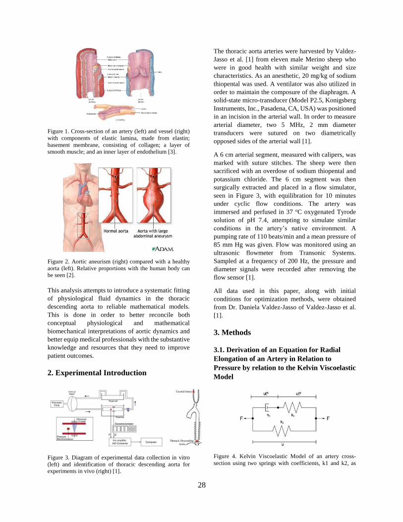
28
Figure 1. Cross-section of an artery (left) and vessel (right)
with components of elastic lamina, made from elastin;
basement membrane, consisting of collagen; a layer of
smooth muscle; and an inner layer of endothelium [3].
Figure 2. Aortic aneurism (right) compared with a healthy
aorta (left). Relative proportions with the human body can
be seen [2].
This analysis attempts to introduce a systematic fitting
of physiological fluid dynamics in the thoracic
descending aorta to reliable mathematical models.
This is done in order to better reconcile both
conceptual physiological and mathematical
biomechanical interpretations of aortic dynamics and
better equip medical professionals with the substantive
knowledge and resources that they need to improve
patient outcomes.
2. Experimental Introduction
Figure 3. Diagram of experimental data collection in vitro
(left) and identification of thoracic descending aorta for
experiments in vivo (right) [1].
The thoracic aorta arteries were harvested by Valdez-
Jasso et al. [1] from eleven male Merino sheep who
were in good health with similar weight and size
characteristics. As an anesthetic, 20 mg/kg of sodium
thiopental was used. A ventilator was also utilized in
order to maintain the composure of the diaphragm. A
solid-state micro-transducer (Model P2.5, Konigsberg
Instruments, Inc., Pasadena, CA, USA) was positioned
in an incision in the arterial wall. In order to measure
arterial diameter, two 5 MHz, 2 mm diameter
transducers were sutured on two diametrically
opposed sides of the arterial wall [1].
A 6 cm arterial segment, measured with calipers, was
marked with suture stitches. The sheep were then
sacrificed with an overdose of sodium thiopental and
potassium chloride. The 6 cm segment was then
surgically extracted and placed in a flow simulator,
seen in Figure 3, with equilibration for 10 minutes
under cyclic flow conditions. The artery was
immersed and perfused in 37 oC oxygenated Tyrode
solution of pH 7.4, attempting to simulate similar
conditions in the artery’s native environment. A
pumping rate of 110 beats/min and a mean pressure of
85 mm Hg was given. Flow was monitored using an
ultrasonic flowmeter from Transonic Systems.
Sampled at a frequency of 200 Hz, the pressure and
diameter signals were recorded after removing the
flow sensor [1].
All data used in this paper, along with initial
conditions for optimization methods, were obtained
from Dr. Daniela Valdez-Jasso of Valdez-Jasso et al.
[1].
3. Methods
3.1. Derivation of an Equation for Radial
Elongation of an Artery in Relation to
Pressure by relation to the Kelvin Viscoelastic
Model
Figure 4. Kelvin Viscoelastic Model of an artery cross-
section using two springs with coefficients, k1 and k2, as

29
well as a dashpot representing dampening phenomena with
dampening coefficient η1.
The force balance of the Kelvin Viscoelastic Model
(Figure 4) is shown in Equation 1.
𝐹 = 𝐹1(𝑠)
+ 𝐹2(𝑠)
(1)
where the forces 𝐹1(𝑠)
and 𝐹2(𝑠)
of the springs relating
to the spring constants k1 and k2 and displacements u1(s)
and u, respectively, are
𝐹1(𝑠)
= 𝑘1𝑢1(𝑠)
(2)
𝐹1(𝑠)
= 𝑘2𝑢 (3)
by Hooke’s Law. Therefore:
𝐹 = 𝑘1𝑢1(𝑠)
+ 𝑘2𝑢 (4)
By rearranging Equation 4 to solve for 𝑢1(𝑠)
, we obtain
Equation 5.
𝑢1(𝑠)
=𝐹
𝑘1−
𝑘2
𝑘1 𝑢 (5)
Due to spring relating to k1 and dashpot relating to η1
lying on the same branch, the forces exerted on each
component must be equal.
𝐹1(𝑠)
= 𝐹1(𝑑)
(6)
With that in mind, and rearranging Equation 2, the
following relation is true:
𝑢1(𝑠)
= 𝐹1
(𝑠)
𝑘1=
𝐹1(𝑑)
𝑘1=
𝜂1
𝑘1
𝑑𝑢1(𝑑)
𝑑𝑡 (7)
Due to the fact that both branches are displaced the
same amount when force F is applied, the following
balance equation is valid:
𝑢 = 𝑢1(𝑠)
+ 𝑢1(𝑑)
(8)
Solving for 𝑑𝑢
𝑑𝑡, in order to receive a differential
equation, albeit nonlinear, of 𝑢 in terms of all other
parameters.
𝑑𝑢
𝑑𝑡=
(𝐹− 𝑢𝑘2
𝜂1)+(
1
𝑘1)(
𝑑𝐹
𝑑𝑡)
1+ 𝑘2𝑘1
(9)
Equation 9 then allows us to generalize the parameter
for force, F, applied at two diametrically opposed
points on the arterial wall to pressure, P, applied along
the entire circumference of the arterial wall. Also, we
can generalize the distention,𝑢, of the arterial diameter
along which F is applied to radial arterial elongation,
ε. These generalizations, when applied to Equation 9,
give Equation 10.
𝑑𝜀
𝑑𝑡=
(𝑃− 𝜀𝑘2
𝜂1)+(
1
𝑘1)(
𝑑𝑃
𝑑𝑡)
1+ 𝑘2𝑘1
(10)
Solving this differential equation thus allows the
determination of ε of an artery in relation to P.
3.2. Determination of a Mathematical Model
for Pressure
In order to determine P as a function of time, the ovine
pressure data obtained from Valdez-Jasso et al. [1]
must first be plotted and analyzed. Due to its
oscillatory nature, the following model was applied:
𝑃 = asin(𝜔𝑡) + 𝑏𝑐𝑜𝑠(𝜔𝑡) + 𝑐 (11)
First, the amplitude values of each peak and the time
distance between them were found, which gave the
period. Then the inverse of the period was taken to find
frequency. Then both sides of the resulting linear
algebraic equation were multiplied by AT in order to
create a pseudo-square matrix to find the coefficients
of sinusoids “a” and “b” as well as amplitude shift “c”.
The final result can be seen in Equation 12.
[𝑎𝑏𝑐] = (𝐴𝑇𝐴)−1𝐴𝑇𝑃𝐷𝑎𝑡𝑎 (12)
3.3. Fitting of a Pressure Model Parameters
Using the Gauss-Newton Method
The Gauss-Newton Algorithm, which attempts to
close the gap between an analytical model and
observed data by modifying values of the model’s
parameters, was then implemented in by defining an
initial vector of parameters a, b, c, and ω. Two loops,
one inside the other, were run. The outer loop dealt
with the iterations of the Gauss-Newton method,
updating the parameter vector, θ, each time. The inner
loop assembled the matrices of the Jacobian and
Residual.

30
The general formula for the Jacobian matrix can be
seen in Equation 13. Each new row has a different P
value corresponding to the use of a different time
point. Note that there are “n” total number of time
points. The columns of the Jacobian matrix contain
derivatives of P with respect to a, b, c, and 𝜔, seen in
Equation 13.
𝐽 =
[ 𝜕𝑃1
𝜕𝑎
𝜕𝑃1
𝜕𝑏
𝜕𝑃1
𝜕𝑐
𝜕𝑃1
𝜕𝜔𝜕𝑃2
𝜕𝑎
𝜕𝑃2
𝜕𝑏
𝜕𝑃2
𝜕𝑐
𝜕𝑃2
𝜕𝜔
⋮ ⋮ ⋮ ⋮𝜕𝑃𝑛
𝜕𝑎
𝜕𝑃𝑛
𝜕𝑏
𝜕𝑃𝑛
𝜕𝑐
𝜕𝑃𝑛
𝜕𝜔 ]
(13)
The residual is the difference between the data and the
model at any given time point. The general equation
for the residual is shown by Equation 14.
𝑟 = [
𝑃𝑟𝑒𝑠𝑠𝑢𝑟𝑒𝐷𝑎𝑡𝑎1 − 𝑃1
𝑃𝑟𝑒𝑠𝑠𝑢𝑟𝑒𝐷𝑎𝑡𝑎2 − 𝑃2
⋮𝑃𝑟𝑒𝑠𝑠𝑢𝑟𝑒𝐷𝑎𝑡𝑎𝑛 − 𝑃𝑛
] (14)
The resulting equation for the updating of θ values can
be seen in Equation 15.
𝜃𝑖+1 = 𝜃𝑖 + (𝐽𝑇𝐽)𝐽𝑇𝑟 (15)
Substituting the parameters within θ into Equation 11
gives a Pressure vector with optimized parameter
values. The pressure data, model, and Gauss-Newton
optimized model are shown versus time in Figure 5,
which is found in the Results Section.
Cross-sectional area of the aorta was found using data
of the diameter of ovine aorta, obtained using Valdez-
Jasso et al. [1] through Equation 16.
𝐴 = 𝜋 (𝑑
2)
2
(16)
Where “A” represents cross-sectional area and “d”
represents diameter. Cross-sectional area was then
plotted as a function of time, and can be seen in Figure
6 in the Results Section.
3.4. Optimization of Kelvin Viscoelastic
Model Parameters
The initial values of parameters 𝜂1, 𝑘1, and 𝑘2
obtained from Dr. Daniela Valdez-Jasso of Valdez-
Jasso et al. [1] can be seen in Table 1.
Table 1. Initial and optimized values of parameters used in
the Kelvin Viscoelastic Model
Parameter Initial Value Optimized Value
k1 40 N/m -0.1345 N/m
k2 60 N/m 327.1812 N/m
η1 20 (N * sec) / m 27.5135 (N * sec) / m
The Matlab function “fminsearch”, which serves the
same purpose of optimizing parameters in a similar
way as the Gauss-Newton Method. The difference is
that it is more convenient for coding purposes to use
fminsearch over the Gauss-Newton Method. The
function fminsearch is an unconstrained optimization
regime, meaning a time range does not need to be
specified, in order to optimize Equation 10. The initial
values were entered as arguments into the fminsearch
function as well as a function which solved Equation
10 using the Matlab function “ode45”. The output of
this function was the objective function as seen in
Equation 17.
𝑂𝑏𝑗𝐹𝑢𝑛 = ∑ (𝐴𝑟𝑒𝑎𝐷𝑎𝑡𝑎𝑗 − 𝐴𝑗𝑛𝑗=1 )2 (17)
Thus the function fminsearch minimizes the objective
function which represents the difference between the
cross-sectional area calculated using the aorta
diameter data and the area calculated by solving
Equation 10 and substituting it into Equation 18.
𝐴(𝑡) = 𝜀𝐴𝑚𝑖𝑛 + 𝐴𝑚𝑖𝑛 (18)
where 𝐴𝑚𝑖𝑛 is the smallest cross-sectional area.
The graph of the model of A(t) can be seen in Figure
6 in the results section.
The resulting parameter values in the vector θ were
then substituted again into Equation 10 when solving
for 𝜀 using the Ode45 solver. The value of 𝜀 with
optimized values, shown in Table 1, was then
substituted into Equation 18 in order to solve for the
cross-sectional area. The results are shown in Figure
6.
4. Results
A non-stiff method, meaning a numerically stable
method, of numerical integration of differential
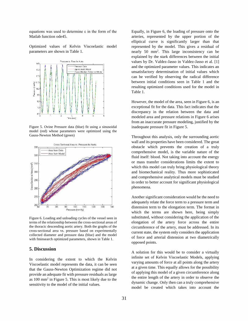
31
equations was used to determine ε in the form of the
Matlab function ode45.
Optimized values of Kelvin Viscoelastic model
parameters are shown in Table 1.
Figure 5. Ovine Pressure data (blue) fit using a sinusoidal
model (red) whose parameters were optimized using the
Gauss-Newton Method (green)
Figure 6. Loading and unloading cycles of the vessel seen in
terms of the relationship between the cross-sectional areas of
the thoracic descending aortic artery. Both the graphs of the
cross-sectional area vs. pressure based on experimentally
collected diameter and pressure data (blue) and the model
with fminsearch optimized parameters, shown in Table 1.
5. Discussion
In considering the extent to which the Kelvin
Viscoelastic model represents the data, it can be seen
that the Gauss-Newton Optimization regime did not
provide an adequate fit with pressure residuals as large
as 100 mm2 in Figure 5. This is most likely due to the
sensitivity to the model of the initial values.
Equally, in Figure 6, the loading of pressure onto the
arteries, represented by the upper portion of the
elliptical curve is significantly larger than that
represented by the model. This gives a residual of
nearly 50 mm2. This large inconsistency can be
explained by the stark differences between the initial
values by Dr. Valdez-Jasso in Valdez-Jasso et al. [1]
and the optimized parameter values. This indicates an
unsatisfactory determination of initial values which
can be verified by observing the radical difference
between initial conditions seen in Table 1 and the
resulting optimized conditions used for the model in
Table 1.
However, the model of the area, seen in Figure 6, is an
exceptional fit for the data. This fact indicates that the
discrepancy in the relation between the data and
modeled area and pressure relations in Figure 6 arises
from an inaccurate pressure modeling, justified by the
inadequate pressure fit in Figure 5.
Throughout this analysis, only the surrounding aortic
wall and its properties have been considered. The great
obstacle which prevents the creation of a truly
comprehensive model, is the variable nature of the
fluid itself: blood. Not taking into account the energy
or mass transfer considerations limits the extent to
which this model can truly bring physiological theory
and biomechanical reality. Thus more sophisticated
and comprehensive analytical models must be studied
in order to better account for significant physiological
phenomena.
Another significant consideration would be the need to
adequately relate the force term to a pressure term and
distension term to the elongation term. The format in
which the terms are shown here, being simply
substituted, without considering the application of the
elongation of the artery force across the entire
circumference of the artery, must be addressed. In its
current state, the system only considers the application
of force and arterial distension at two diametrically
opposed points.
A solution for this would be to consider a virtually
infinite set of Kelvin Viscoelastic Models, applying
varying amounts of force at all points along the artery
at a given time. This equally allows for the possibility
of applying this model of a given circumference along
the entire length of the artery in order to observe the
dynamic change. Only then can a truly comprehensive
model be created which takes into account the

32
multitude of phenomena along the entire length of an
artery.
6. References
1. Valdez-Jasso, D., D. Bia, Y. Zocalo, R.L.
Armentano, M.A. Haider, M.S. Olufsen. Linear
and Nonlinear Viscoelastic Modeling of Aorta
and Carotid Pressure-Area Dynamics Under In
Vivo and Ex Vivo Conditions. Annals of Biomed.
Engr. 39(5): 1438-1456, 2011.
2. (2005) Abdominal Aortic Aneurysm Screening &
Treatment Options. [Online]. Available:
http://www.torontoendovascularcentre.com/pat/b
ackground.html
3. Carrion, J. (2011). Anatomia y Fisiologia
Cardiaca. [Online]. Available:
http://es.slideshare.net/jorgeluis19/anat-corazon

Superiority of Proton CT as an Alternative to X-ray CT for use in Proton Therapy Treatment Planning
James [email protected]
AbstractProton computed tomography (pCT) is an in-development imaging technique that offers potentialbenefits to external beam therapy treatment planning. Like X-ray CT (xCT), pCT utilizes iterativealgorithms to facilitate image reconstruction based on energy attenuation. However, pCTfunctions by sending ~200MeV proton beams through the patient as opposed to x-rays, forming animage based on position, and residual energy of exiting protons. While research has shown bettercontrast resolution and lower radiation dosage in pCT when compared to standard xCT, multiplecoulomb scattering (MCS) of protons in the tissue leads to a steep reduction in spatial resolution.This paper reviews the essential physics, technology and techniques underlying pCT imaging,analyzing its feasibility as an alternative to the current standards of xCT in proton therapyplanning.
Keywords: Proton CT, Computed Tomography, Medical Imaging, Proton Therapy, MultipleCoulomb Scattering
1. Introduction
With the rapid advancement of cancer therapy intoday’s medicine, demand for the refinement ofassociated instrumentation and technology is at anall-time high [2]. One of the cutting-edge techniques,proton therapy, utilizes precisely tuned proton beamsin order to irradiate tumors while minimizing damageto surrounding tissues. Calibration of radiationdosage during this procedure is essential and reliesheavily on imaging techniques to determine thestopping power (SP) through the patient. Currently,SP maps are assembled from 3D images acquiredthrough X-ray computed tomography (xCT) [1].However, tissue interactions differ significantlybetween X-rays and protons (Figure 1), requiringtransformation using a calibration curve [5].Measurements consistently return 3-4% error inelectron density calculation due to this translation [3].This source of error can be ameliorated by directlymeasuring energy attenuation using proton computedtomography (pCT).
pCT was first proposed by Nobel laureate AllanCormack, one of the pioneers of xCT, in 1976.Efforts to study the potential of pCT continued intothe 1980’s but poor proton beam quality and slowdata acquisition time halted the interest of theimaging community. Combined with the increasingutilization of proton therapy in cancer treatment,advancements in particle physics, instrumentationand computing in the last decade have brought aresurgence of research on the subject [2].
Figure 1. X-ray attenuation (a) and proton energy loss (b)through biological tissues [5].
Much like xCT, pCT measures and records energyattenuation of beams projected through the patientover 360 degrees. Stored data is then formed into amatrix and an image is reconstructed using filteredback projections or other iterative algorithms [6].Though pCT corrects for errors in electron densitymeasurements, image spatial resolution isdeteriorated by multiple coulomb scattering (MCS)of charged particles passing through matter. Also,despite advancements in detection and computingtechnology, data-taking rate is still too slow for use ina clinical setting [6]. The following sections review

the intricacies of pCT imaging and examine itsefficacy as an alternative to the standards of xCTtreatment planning in proton therapy.
2. Proton Therapy
Proton therapy is a type of external beam radiationtherapy (EBRT) that is used in the treatment of awide variety of cancers [1]. The most common formof EBRT uses a beam of photons that easily passthrough biological tissues to damage cancerous cells.Although the system is adjusted to deliver the lowesteffective dose, photon beams do not discriminatebetween tissue types and damage all healthy tissuessurrounding the tumor [8].
Unlike photons, protons are particles that have a massof roughly 1800 times that of an electron [8]. Due totheir size, protons passing through a material areslowed and can be eventually stopped inside matter.After a particle has stopped, it has the opportunity tointeract with surrounding cells, causing ionization ofmolecules and damage to DNA. This property offersthe potential to calibrate beam energies relative to theSP of the cancerous area, sparing healthy tissueslocated on the distal side of the tumor [8].
The energy deposit of protons is characterized by anentrance plateau. At the end of this curve, there is apoint at which a majority of the particle’s energy isattenuated over a short distance referred to as theBragg peak [2]. Knowledge of the Bragg peak isessential to proton therapy because it allowsphysicians to ensure that particles are stopped withinthe desired area. As modeled in Figure 2, modifiedbeams begin at low energies that gradually increaseto cover the entirety of the tumor [8].
Presently, xCT uses attenuation of photons in order toestimate electron density of tumors. Unfortunately,since there is no unique relationship between thephysical interaction processes of protons and photonsdata must be transformed using a calibration curve,posing a major source of potential error [2]. xCT alsofrequently provides poor contrast between canceroustumors and surrounding healthy tissue, makingradiographs virtually useless in proton therapy.Development of a clinical CT system that usesprotons instead of X-rays to determine SP is the nextstep in advancing proton therapy.
Figure 2. Photon beams start at high energy and areattenuated as they pass through matter. Proton beams arecalibrated based on the Bragg peak to stop completely andrelease energy in a localized area [8].
3. Physical Principles of pCT
Proton CT measures both the position and residualenergy of protons exiting an object. The overallchange in energy, dE, over the path length, s, can bederived using the Bethe-Bloch formula [6]:
dEds =
N Aρ Z 42 e4
Ame c2β2 (ln ( 2me c2 β2
I (1−β2))−β2) (1)
This equation can be grouped into two functions:ne(x,y,z) is the electron density of the material, whichdetermines the relative SP, and f[I,β(E)] depends onthe ionization potential of the material, I, and incidentproton velocity, β [6].
dEds =ne (x , y , z ) f [ I ,β ,(E)] (2)
Using separation of variables:
∫E ¿
E out dEf [ I ,β, (E )]
=∫ ne (x , y , z )ds (3)
Ein is a constant, determined by the energy of theincident proton beam. Proton beam energies used intherapy typically range from 70-250 MeV, dependingon the size, type and location of the tumor [1-7]. Eq.3 can be approximated by the discrete sum of relativeSP times traversing the path of the particle [6].
While superior to xCT in SP measurements, steepreductions in spatial resolution have been attributedto MCS [1]. In fact, 200 MeV protons passingthrough relatively thick objects (20cm) are subject toMCS angles of up to 40mrad, corresponding to adisplacement of ~3mm [7]. Projected scatter angle isapproximated using proton velocity and momentum,

β and p, in relation to the thickness of the material inunits of radiation length, x/X0 [3]:
θmcs=13.6 MeV
βcp z√ xX 0
[1+ .038 ln xX 0
] (4)
X0 is determined as the inverse of the sum of thefractions by weight of each material traversed, w j, perunit material radiation length, Xj [3]:
1X 0
=∑w j
X j (5)
Table 1 shows the potential of these equations inMCS angle approximation when compared to actualvalues using a phantom hand model in Plautz et al.Angles were calculated to within ~±1mrad ofobserved values [3].
Table 1. Expected vs. observed MCS angles of 5 regions ofinterest in a phantom hand model [3].
4. Apparatus
The pCT apparatus is comprised of a beam generator,a tracking system and a calorimeter coupled with asilicon photomultiplier, shown in detail in Figure 3[7]. Protons are passed through tracker boardsequipped with sensors that record the entrance pointof each single event. Downstream, another pair oftracker boards and sensors records the position of theexiting particle. This data is interpreted using MonteCarlo algorithms to compute a most likely path(MLP) trajectory through the object [7]. Protons thencontinue into a calorimeter composed of scintillatingcrystals located behind the downstream tracker.Particles are ultimately stopped within the crystalsand residual energy is recorded.
4.1 Trackers
The detectors consist of 400 µm thick silicon discsensors implanted with coordinate strips. Foursensors are cut into squares and mounted in a slightlyoverlapping square pattern onto tracker boards [2].Each tracker plane consists of two identical trackerboards mounted back-to-back and rotated 90 degreesso that the impact point can be pinpointed on the x,y
plane. Sensors from each plane are wired toapplication specific integrated circuits (ASIC) andtransmitted on low-voltage differential signal (LVDS)lines [4]. With the current setup, error contributed byMCS on MLP has been reduced to below .1mm(Figure 4) [1].
Figure 3. Proton CT apparatus: (a) crystal calorimeter (b)front-end tracker board (c) silicon sensor (d) digital trackerboard (f) phantom object (g) beam generator (p1-p4)identical tracker planes
Figure 4. MLP error contributions using 200 MeV protonenergy and 20 cm phantom [1].
The silicon sensors used in the apparatus wereoriginally designed in the development of the GammaRay Large Area Space Telescope (GLAST).Therefore, specifications for the pitch resolution(228µm), front-end electronics and readoutcontrollers were already optimized for use in datacollection [2]. Digital data from the circuits is readoutby field programmable gate arrays (FPGA) to be sentto an event builder and processed by a host PC [4].
Region Expected(mrad)
Observed (mrad)
1 17 17.8 ± 0.92 15 14.1 ± 0.93 11 12.3 ± 0.74 10 10.3 ± 1.35 5 5.2 ± 0.4

4.2 Calorimeter
The pCT calorimeter is comprised of rectangularscintillating crystals, stacked and adhered together ina matrix. Each crystal has a 3cm x 3cm square cross-section and a depth greater than 10cm to ensure noparticle is able to pass through undetected [1].Chemical composition of the calorimeter crystals ischosen based on its emission wavelength maximumto best match the sensitivity spectrum of thephotodiode. Both YAG:Ce (Yttrium AluminumGarnet activated by Cerium) and CsI(Tl) (Thalliumactivated Cesium iodide) have emission wavelengthmaximums of 550nm and fast emission decayconstants, making them ideal for the siliconphotodiodes and a high flux environment [1,2].Crystals are fabricated with rough surfaces on everyside except for where it is coupled with thephotodiode. Although cutting a clean edge on thissurface degrades light output of the crystal, it resultsin a more uniform response [2]. Immediatelyfollowing detection by photodiodes, a preamplifierand pulse shaper prepare signals to be sent to ananalog to digital converter (ADC) for data collection[4].
4.3 Data Acquisition
The data acquisition process begins with thedigitization of position and energy data. An eventbuilder is interfaced directly with the calorimeter andthe FPGAs of the tracking system where it isorganized to be processed by the host computer. Ablock diagram of the data flow is referenced in Figure5 [4]. While data collection for residual energy isstraight forward, position data must be furtherprocessed using Monte Carlo algorithms for MLPreconstruction [7]. Monte Carlo programscontinuously generate randomized numericalexperiments based on mathematical expressions.While proven to be very effective in simulation ofphysical events, iterations from the order ofthousands or even millions can be necessary to returndesired precision. Reconstruction of MLP data cantake up to 12 hours due the sheer size of simulateddata required for each event [7]. In order to beapplicable for clinical use, this time needs to becomea matter of minutes through reduction of data size orgreater processing power [2].
Figure 5. Diagram of pCT data flow [4].
5. Conclusion
Through the direct measurement of residual protonenergy, pCT imaging offers superior electron densityestimation while also reducing radiation exposureduring treatment planning. While MCS initiallycaused a major reduction in spatial resolution, MLPparticle trajectory approximation using Monte Carlomethods has proven to reduce error sufficiently tocompare with the quality of xCT. Although dataacquisition time is still too slow for use in a clinicalsetting, its potential to reduce damage to surroundinghealthy tissues during proton therapy should drivefuture research. Studies are currently being done toreduce data size and ultimately allow for faster dataacquisition using presently available processingpower. Use of plastic scintillators in both thecalorimeter and tracking planes may also have thepotential to reduce the imaging time to as low as tenminutes [2]. As pCT research progresses, furthertesting to determine reconstruction accuracy and bothspatial and density resolution limitations over a largerfield of view is necessary [1].
6. References
1. Civinini C., M. Bruzzi, M. Bucciolini, M.Carpinelli, G.A.P. Cirrone, G. Cuttone, D. LoPresti, S. Pallotta, C., Pugliatti, N. Randazzo, F.Romano, M. Scaringella, V. Sipala, C.Stancampiano, C. Talamonti, M. Tesi, E. Vanziand M. Zani. “Recent Results on theDevelopment of a Proton ComputedTomography System.” Nuclear Instruments &Methods in Physics Research Section A 732:573-576, 2013

2. Coutrakon, G., V. Bashkriov, F. Hurleym R,Johnson, V. Rykalin, H. Sadrozinski and R.Schulte. “Design And Construction of The 1st
Proton CT Scanner.” AIP ConferenceProceedings 1525:327-331, 2013
3. Plautz T,. B. Bashikrov, V. Feng, F. Hurley, R.P.Johnson, C. Leary, S. Macafee, A. Pumb, V.Rykalin, H.F.W. Sadrozinski, K. Schubert, R.Schulte, B. Schultze, D. Steinberg, M. Witt andA. Zatserklyaniy. “200 MeV Proton RadiographyStudies with a Hand Phantom Using a PrototypeProton CT Scanner.” Transactions On MedicalImaging 33: 875-881, 2014
4. Sadrozinski, H.F.-W., V. Bashkirov, R.F. Hurley,R.P. Johnson, S. Macafee, A. Plumb, R.W.Schulte, D. Steinberg and D. Zatserklyaniy.“Development of a Head Scanner for ProtonCT.” Nuclear Instruments & Methods in PhysicsResearch Section A 699: 205-210, 2013
5. Sadrozinski, H.F.-W., V. Bashkirov, M. Bruzzi,L.R. Johnson, B. Keeney, G. Ross, R.W. Schulte,A. Seiden, K. Shahnazi, D.C. Williams and L.Zhang. “Issues in Proton ComputedTomography.” Nuclear Instruments & Methodsin Physics Research Section A 511:275-281,2003
6. Saraya Y., T. Izumikawa, J. Goto, T. Kowasakiand T. Kimura. “Study of Spatial Resolution ofProton Computed Tomography Using a SiliconStrip Detector.” Nuclear Instruments & Methodsin Physics Research Section A 735: 485-489,2014
7. Scarringella, M,. M. Brianzi, M. Bruzzi, M.Bucciolini, M. Carpinelli, G.A.P. Cirrone, C.Civinini, G. Cuttone, D. Lo Presti, S. Pallotta,C., Pugliatti, N. Randazzo, F. Romano, V. Sipala,C. Stancampiano, C. Talamonti, M. Tesi, E.Vanzi and M. Zani. “The PRIMA (ProtonIMAging) collaboration: Development of aProton Computed Tomography Apparatus.”Nuclear Instruments and Methods in PhysicsResearch Section A 173:573-57, 2013
8. Wisenbaugh, E.S., P.E. Andrews, R.G. Ferrigni,S.E. Schild, S.R. Keole, W.W. Wong and S.A.Vora. “Proton Beam Therapy for LocalizedProstate Cancer 101: Basics, Controversies, andFacts.” Reviews in Urology 16:67-75, 2014

38
MODELING THE EFFECTS OF TEMPERATURE CHANGES ON
CARDIAC PURKINJE FIBERS Martin Strama
Abstract Purkinje fibers (PFs) rapidly conduct electrical impulses in the cardiac conduction system to initiate
the normal excitations of the ventricles. Abnormalities in the PF system caused by temperature
changes may result in abnormal excitation of the heart, which can lead to ventricular bradycardia,
tachycardia, or fibrillation. The Noble PF (NPF) model is utilized to model the effects of
temperature changes on cardiac PFs. As temperature is decreased below body temperature, the
number of action potentials (APs) and firing frequency decrease. Conversely, as the temperature is
increased, the previous properties increase and the waveforms become distorted. Although the NPF
model produces the long plateau duration characteristic of cardiac PFs, the model limits the sodium
channel to both the upstroke and plateau phase of the AP. Since the PF system is critical in both
normal ventricular excitation and fatal ventricular arrhythmias, accurately modeling PF behavior
is essential for future cardiac ventricular models as well as engineering ventricular grafts.
Keywords: Neural Engineering, Purkinje Fibers, Noble Model, Hodgkin-Huxley Model
1. Introduction
The cardiac conduction system (CCS) is a specialized
electrical system that regulates the coordinated
contraction of the heart by propagating electrical
impulses through a network of specialized myocardial
cells [1, 2]. The CCS of the adult mammalian heart
comprises the sino-atrial (SA) node, the internodal
tracts, the atrio-ventricular (AV) node, the His bundle,
its right and left branches, and the network of Purkinje
fibers (PFs) as shown in Figure 1 [1, 2, 3]. The SA
node spontaneously generates electrical pulses within
the heart and thus is often described as the principal
pacemaker of the heart. The electrical pulses are
dispersed as waves of electrical excitation over the
atria, through the AV node into the ventricles, to the
His bundle, its right and left branches, and into the PFs
– the terminal part of the CCS. The PFs are electrically
connected to the ventricular muscle, and their main
function is to distribute the depolarization signal to the
myocardium in order to facilitate ventricular
excitation and contraction.
The previously described pattern of excitation within
the CCS corresponds to the normal sequence of
cardiac activation. Abnormalities in the excitation
pattern may lead to potentially fatal cardiac
arrhythmias and can occur in any element of the
conduction pathway [2]. The PF system is considered
to be a critical component in the development and/or
maintenance of cardiac arrhythmias such as
ventricular bradycardia, tachycardia, and fibrillation
[2, 4]. Since the PF system is critical in both normal
ventricular excitation and fatal ventricular
arrhythmias, modeling PF behavior is essential for
future cardiac ventricular models.
Herein, the Dennis Noble PF (NPF) model will be
utilized to simulate and characterize the behavior of
PFs [5]. Initially, the NPF model will be compared to
the classic Hodgkin-Huxley (HH) model by applying
various input stimulus currents to each model. Next,
the PFs will be subjected to various human
physiological temperatures. Lastly, the PFs will
receive various input stimulus currents at a constant
temperature in order to observe the effects on action
potential (AP) firing frequency.
Figure 1. The cardiac conduction system of the mammalian
heart [3]. Each myocardial component produces a
characteristic voltage response as the electrical impulse
propagates through the heart. The characteristic voltage
response of the Purkinje fibers is highlighted.

39
2. Methods
The PF model under investigation is the NPF model,
the first cardiac electrophysiological model developed
for PFs. The NPF model was based on the HH model
of the AP in the squid giant axon, and modified to
reproduce the long plateau duration of cardiac PF APs
shown in Figure 1.
Briefly, the HH model utilizes the parallel
conductance model to describe the major ionic
conductances in the squid giant axon as shown in
Figure 2A [6]. The model proposed that the nonlinear
voltage-gated sodium (Na+) and potassium (K+)
conductances were controlled by gating particles –
specifically the m-gate and h-gate for Na+, and the n-
gate for K+. When combined with the equations of
cable theory, the HH model could accurately
reproduce the shape and size of the AP, impedance
changes, conduction velocity, and the ionic exchanges
of the squid giant axon.
Noble modified the HH model to account for the
natural excitable membrane behavior of PFs as shown
in Figure 2B [5]. As opposed to the squid giant axon,
depolarization decreases the K+ permeability of the
membrane and thus lowers the membrane conductance
to K+. During large depolarizations, part of the
decrease in K+ permeability appears to be only
transient, and the K+ current slowly increases during
the passage of the depolarizing current. Thus, the NPF
model assumes that the K+ current flows through two
types of channels as seen in Figure 2B. In one of the
K+ channels, the K+ conductance gK1 is assumed to be
an instantaneous function of the membrane potential
and falls when the membrane is depolarized. In the
second type of K+ channel, the K+ conductance gK2
slowly rises when the membrane is depolarized. As
seen in Figure 2B, the two types of K+ channels are
represented by two parallel rectifiers in series with the
K+ Nernst potential. The K+ conductance gK1 is
represented by a rectifier that easily passes inward
current, while gK2 is represented by a rectifier which
easily passes outward current. Furthermore, the NPF
model incorporates a chloride (Cl-) current instead of
a leak current and a background Na+, neither present
in the HH model.
2.1 Calculations
The NPF model conforms to the convention usually
adopted in experimental work with intracellular
electrodes, where the potential Em is the potential of
the inside with respect to the outside. As a result,
positive currents are therefore outward and not inward,
as in the HH model.
The NPF model utilizes four state variables:
membrane potential Vm, slow K+ activation gate n, Na+
activation gate m, and Na+ inactivation gate h. All
analyses and computations were done using custom
MATLAB scripts (MATLAB R2014a, MathWorks).
The complete NPF model is listed below. (See ref. [6]
for the complete HH model.)
0m ion mdV dt I J C (1)
, ,ion Na K Cl b Na bJ J J J J (2)
3mNa NaNaJ g m h V E (3)
1 2
mK K K KJ g g V E
(4)
, , mCl b Cl b ClJ g V E (5)
Figure 2. A. Equivalent circuit of the Hodgkin-Huxley (HH)
model [6]. The HH model utilizes the parallel conductance
model to describe the lipid bilayer, nonlinear voltage-gated
Na+ and K+ ion channels, and linear leak ion channel. B.
Equivalent circuit of the Noble Purkinje fiber (NPF) model
[5]. The NPF model expands on the HH equivalent circuit
by assuming that the K+ current flows through two nonlinear
channels and includes background Na+ and Cl- currents (not
shown).
A.
B.

40
, , mNa b Na b NaJ g V E (6)
1
exp 90 50
0.015exp 90 60
mK K
m
g g V
V
(7)
4
2KK
g g n (8)
0.1 48 1 exp 48 15m m mV V (9)
0.12 8 exp 8 5 1m m mV V (10)
0.17exp 90 20h mV (11)
1 1 exp 42 10h mV (12)
0.0001 48 1 exp 50 10n m mV V (13)
0.002exp 90 80n mV (14)
1m m Cdm dt m m T (15)
1h h Cdh dt h h T (16)
1n n Cdn dt n n T (17)
3^ 37 10C CT T (18)
Equation 1 represents the characteristic equation for
the NPF circuit shown in Figure 2B. The ion current
Jion (µA/cm2) in Equation 2 is the sum of each
individual ion channel current in the NPF model.
Equations 3 – 6 describe the fast Na+ current, the K+
current, the background Cl- current, and the
background Na+ current (not shown in Figure 2B),
respectfully. Equation 7 and Equation 8 characterize
the pacemaker K+ conductance gK1 and outward
rectifying K+ conductance gK2, respectfully. Equations
9 – 14 define the opening (α) and closing (β) rates
(msec-1) for gates m, h, and n, respectfully. Equations
15 – 17 detail the time dependence for each respective
gate. To model the electrical behavior of PFs when
subjected to various human physiological
temperatures, the gate rates were scaled by a scaling
factor φ(TC) defined in Equation 18 [7]. Table 1
presents the simulation parameters utilized to model
the electrical behavior of the PFs. The same values
were utilized where applicable in the HH model.
Table 1. Simulation parameters for the NPF model.
Variable Value Unit
Membrane Potential, Vm,0 -81.6 mV
Input Current, I0 {0,5,15,50}* µA
0.4**
Na+ Nernst Potential, ENa+ 40 mV
K+ Nernst Potential, EK+ -100 mV
Cl- Nernst Potential, ECl- -60 mV
Na+ Conductance, Nag 400 mS
K+ Conductance, Kg 1.2 mS
Background Cl-
Conductance, ,Cl bg 0.075 mS
Background Na+
Conductance, ,Na bg 0.14 mS
Membrane
Capacitance, Cm 12 µF/cm2
Na+ activation gate, m0 0.04338 msec-1
Na+ inactivation gate, h0 0.85218 msec-1
K+ activation gate, n0 0.60888 msec-1
Temperature, TC {30,34,37,40,44} ̊C
Time, t [0 2] sec * The following input currents were utilized to compare the NPF
model to the HH model and to obtain the action potential firing
frequency for each temperature. ** The following input current was utilized and remained constant
when subjecting the PFs to various temperatures. Variables with the
number zero indicate initial values at time equal to zero.
3. Results
3.1 Comparing the Noble Purkinje Model to
the Hodgkin-Huxley Model
Both the NPF model and HH model spontaneously
elicit an AP when no input stimulus current is applied
as shown in Figure 3. Only the NPF model produces
characteristic PF AP waveforms. Conversely, the HH
model produces a single spike and fails to refract
because the Na+ inactivation h-gate immediately
reaches a probability of zero, which indicates that the
inactivation gate is closed. When the input stimulus
current is increased to 5 µA, the NPF waveform
becomes distorted and produces a single PF AP due to
the decreased h-gate probability. The NPF gate
probabilities approach the HH gate probabilities for
each respective gate as the input stimulus current is
increased. As a result, the NPF waveform
progressively resembles the HH waveform.

41
3.2 Analyzing the Effects of Temperature on
Purkinje Fibers
Altering temperature has a considerable impact on the
PF waveform as seen in Figure 4. As temperature is
decreased below body temperature (BT, 37 ̊C), the
number of APs decrease in a 2 sec time interval, peak
amplitudes increase, and gate probabilities lengthen.
Furthermore, transient oscillations in AP firing
frequency occur as input stimulus current is increased.
Conversely, as temperature is increased above BT, the
number of APs increase in a 2 sec time interval, peak
amplitudes decrease, and gate probabilities shorten. In
addition, the APs become distorted and no sharp peaks
occur. Furthermore, the transient oscillatory nature
seen in waveforms below BT diminish and a linear-
like relationship forms.
4. Discussion
The NPF model utilizes three ionic components
similar to the HH model: a nonlinear Na+ term, a
nonlinear K+ term that undergoes rectification, and a
nonspecific linear anion term. Thus the resemblance of
the NPF model to the HH model at high input
stimulating currents is no coincidence.
Ion currents change at different temperatures and
produce large differences in the APs. Temperature can
accelerate or decelerate gate kinetics by modifying the
rate constants governing the channel conductances.
When the temperature of the PFs are not at BT,
abnormal waveforms of varying AP firing frequencies
are produced that modify the QRS complex shown in
Figure 1 to produce cardiac arrhythmias. Although
temperature can directly affect the gate kinetics,
temperature also modifies the current as seen in the
Goldman-Hodgkin-Katz (GHK) current equation.
0 µA
5 µA
15 µA
50 µA
Figure 3. The Nobel Purkinje fiber (NPF) model compared to the Hodgkin-Huxley (HH) model. The left panel shows the voltage
behavior and the right panel shows the gate behavior. Both models spontaneously fire when no input stimulus current is applied.
The NPF model produces the characteristic PF action potentials seen in Figure 1, while the HH model produces a single spike and
does not refract. As the input stimulus current is increased, the NPF gate probabilities approach the HH gate probabilities for each
respective gate, and as a result, the NPF waveform progressively resembles the HH waveform.

42
Implementing the GHK current equation may produce
more accurate results.
Although the NPF model reproduces the long plateau
duration of cardiac PFs, the model functions because
the voltage range of the Na+ current was greatly
extended by reducing the voltage dependence of the
Na+ activation process [2, 8]. As a result, Na+ is
responsible for both the upstroke and plateau phase of
the PF AP waveform, as seen in the gate probability
graphs. Thus, the Na+ current performs the functions
of both the Na+ and calcium Ca2+ channels, and the PF
AP is maintained by a balance between inward Na+
and outward K+ currents. Therefore, the original NPF
model does not accurately model the cellular
physiology of the heart because of the lack of Ca2+
channels. Nevertheless, the NPF model continues to
serve as the foundation for advanced mathematical
models of cardiac cells [8, 9]. Furthermore, accurately
modeling PF behavior at various physiological
relevant temperatures will be essential for future
cardiac ventricular models as well as engineered
ventricular grafts for in vivo surgical replacements.
5. Acknowledgement
The author would like to thank James Patton, Ph.D.,
and Yazan Abdel Majeed, B.S., for their contributions
throughout this research.
6. References
1. Sedmera, D. and R. G. Gourdie. Why do we have
purkinje fibers deep in our heart? Physiol.
Res.63(Suppl. 1): S9-S18, 2014
A.
B.
Figure 4. The effects of temperature on Purkinje fibers
(PFs). A. Purkinje fibers (PF) action potential (AP)
waveforms at select physiological temperatures. As the
temperature is decreased below body temperature (BT,
37 ̊C), the number of APs decrease in the specified time
interval. Conversely, the opposite result occurs as
temperature is increased above BT, and the waveforms
become distorted. B. PF gate probabilities at select
physiological temperatures. As the temperature is decreased
below BT, the gate probabilities lengthen. The opposite
result occurs as temperature is increased above BT. C. The
effects of input stimulus current on PF AP firing frequency
for each temperature. At temperatures below BT, increasing
the input stimulus current creates a transient oscillation in
AP firing frequency. At temperatures above BT, the
transient oscillatory nature diminishes and a linear-like
relationship forms. Discontinuities occur after 12 µA due to
the NPF model behaving like the HH model, where the AP
no longer refracts (see Figure 3). The input stimulus current
was made constant at 0.04 µA for simulations in panels A
and B, but was modified for simulations in panel C.
C.

43
2. Tusscher, K. H. W. J. T. and A. V. Panfilov.
Modeling of the ventricular conduction system.
Progr Biophys Molec Biol. 96: 152-170, 2008
3. Barrett, K. E. Conduction system of the heart.
Digital image. Ganong's Review of Medical
Physiology, 24e. The McGraw-Hill Compnies,
2012
4. Ideker, R. E. et al. Purkinje fibers and
arrhythmias. Pacing Clin Electrophysiol. 32(3):
283-285, 2009
5. Noble, D. A modification of the hodgkin-huxley
equations applicable to purkinje fibre action and
pace-maker potentials. J. Physiol. 160: 317-52,
1962
6. Hodgkin, A. L. and A. F. Huxley. A quantitative
description of membrane current and its
application to conduction and excitation in nerve.
J. Physiol. 117: 500-14, 1952
7. Feudel, U. Homoclinic Bifuration in a hodgkin-
huxley model of thermally sensitive neurons.
CHAOS 10.1: 231-39, 2000
8. Cherry, E. M. and F.H. Fenton. Realistic cardiac
electrophysiology modelling: are we just a
heartbeat away? J. Physiol. 588(15): 2689, 2010
9. Sampson, K.J., et al. A computational model of
purkinje fibre single cell electrophysiology:
implpications for the long QT syndrome. J.
Physiol. 588(14): 2643-2655, 2010

44
BIOPSYCHOSOCIAL VARIABLES AND THE EFFECTS ON IMMUNE
SYSTEM: AN ANALYSIS OF THE RELATIONSHIP BETWEEN
NEGATIVE MOOD STATES AND PRO-INFLAMMATORY CYTOKINES Nneka O. A. Ukegbu
Abstract Biological and psychological indicators of stress are thought to influence overall immune function.
For years, scientists have attempted to analyze the responses of the brain to various stressors. What
we call “sickness” is essentially the body’s adaptation to certain biological and psychological
attacks. Psychoneuroimmunology, a developing field of study that deals with brain-behavior-immune
relationships, has been gaining more awareness, but has not been well documented in the context of
the African American population. Evidence suggests that negative mood states such as anxiety and
depression, have adverse effects on immunity and trigger off disease. [5] However, little research has
been done that discusses the strength of the relationship and how negative mood states in African
Americans affect immune function. We know that if a person’s immune system is compromised, health
overall is negatively affected as well. This research seeks to determine the extent to which personality
traits – neuroticism and extra-introversion – exacerbate or buffer biological responses to depression
and anxiety. To answer this question we observed the levels of pro-inflammatory cytokines
(interleukin-1) circulating in the blood. Our analysis was from a subset of data from Howard
University Hospital’s General Clinical Research Center (GCRC), Washington DC.
Keywords: Biopsychosocial Variables, Interleukin-1, Multiple Regression Analysis, Brain-Behavior-
Immune Relationships
1. Introduction
The relationship between biopsychosocial
variables is complex and many sequelae of stress
factors are often not understood. In our study we
selected specific biopsychosocial variables and
tested the relationships among them. We
hypothesized that there would be a significant
positive relationship between negative mood states
and immune response, and that personality traits
would serve as moderator variables to this
relationship. The independent variables we
examined for our research were depression,
anxiety, neuroticism, and extra-introversion. Our
dependent variable was interleukin-1.
In our research we asked the question, “To what
extent do personality traits – neuroticism and
extra-introversion – exacerbate or buffer biological
responses to depression and anxiety?” To answer
this question, we observed the levels of
proinflammatory cytokines (interleukin-1)
circulating in the bloodstream of the participants in
the study. Proinflammatory cytokines are
molecules released by the immune system that
serve the function of intercellular communication.
Signals are sent to the brain to respond to
biological or psychological attacks and regulate
normal body responses. Interleukin-1 (IL-1) is the
cytokine being measured in this study. [4]
Research shows that there is a link between major
depressive disorder (MDD) and proinflammatory
cytokines via a pathophysiological mechanism.
Some studies show that patients who have MDD
have higher levels of interleukin-1β. [3] When
there is an infection, the immune system is alerted
and sends out different kinds of cells that have
their specific functions in responding to the
infection. This is also the case when there is
physical injury to the body. The cells circulate
through the blood and send messages to the brain
to respond to the injury or infection. Since we
observe that chronic stress can also lead to
“sickness”, we seek to find out whether the body
uses similar mechanisms to respond to
psychological stress through the immune system.
Research suggests that there are specific pathways
that are used for responding to injury or infection.
It has been argued that, “physical and
psychological stressors activate the same
bidirectional immune-brain circuits”. [1] There are
specific models that explain these biological
mechanisms, however this is beyond the scope of
this particular research. We are interested in
finding out how these interactions take place when

45
we are dealing with psychological stressors, which
are not as tangible.
2. Materials and Methods
Our independent variables – depression and
anxiety – are the psychological states being
measured. The moderator variables – neuroticism
and extra-introversion – are the personality traits
that we expect to alter the strength of the
relationship seen in the variables. According to the
NEO Personality Inventory, the definition of the
variables is as follows: neuroticism pertains to
individuals prone to psychological stress; anxiety
is the level of apprehension, fear or worry a person
has; depression is the tendency to experience
feelings of guilt, sadness and loneliness; extra-
introversion is the intensity of energy a person
directs outwards or inwards into the social world.
We measured the effects of the independent
variables on the inflammation as indicated by the
levels of interleukin-1.
Our analysis focused on a sample of 150 relatively
healthy African American adults in the
Washington, D.C. Metropolitan Area, recruited
from health fairs, using fliers, and by word-of-
mouth. Data came from a larger study conducted in
the National Minority Organ and Tissue Transplant
Education Program (National MOTTEP), which
examined the profiles of immune functioning in
African Americans. MOTTEP is geared towards
educating and creating awareness about organ and
tissue transplantation in minority communities.
With a preventative approach, MOTTEP creates
programs to shed light on the behaviors and
diseases that ultimately lead to organ
transplantation. [6] We performed a secondary
analysis of a subset of MOTTEP data collected at
Howard University Hospital’s General Clinical
Research Center (GCRC) in Washington, DC. This
data consisted of paper-pencil assessments of the
participants, with scoring levels for the different
mood states and personality variables, including
the NEO Personality Inventory-Revised (NEO-PI-
R) and Beck Depression Inventory. The biological
response variable was measured using blood
samples from the participants. We used multiple
regression analysis to examine the fit of a series of
nested sets of predictors with the goals of: (1)
testing our hypotheses, and (2) identifying the
most efficient model for explaining variation in our
dependent variable, IL-1. (Relevant SPSS
statistical analysis software output is provided in
tables 1 & 2)
Following Baron and Kenny (1986), we examined
the extent to which: (a) the independent variable
(IV) (depression) and the hypothesized mediator
(neuroticism) were significantly correlated; (b) the
hypothesized mediator (neuroticism) and the
dependent variable (DV) (IL-1) were significantly
correlated; (c) the inclusion of the mediator
(neuroticism) as an additional predictor in the
regression of the DV (IL-1) on the IV (depression)
resulted in a decrease in the significance of the
correlation between the IV and DV.
We found that depression and neuroticism were
significantly correlated, r(175) = 0.41, p<0.03;
neuroticism and IL-1 were significantly correlated,
r(172) = 0.25, p<0.002. Finally, we regressed IL-1
on depression and neuroticism simultaneously and
found the inclusion of neuroticism as an additional
predictor resulted in a decrease in the significance
of the correlation between depression and IL-1
from p<0.05 to p>0.37.
3. Results
Table 1.
As expected, depression was significantly
positively related to IL-1 (p<0.03) when the
relationship between the negative mood states
(anxiety and depression) and IL-1 were examined
to test our prediction (refer to Model 1 in the first
SPSS analysis table); however, anxiety and IL-1
were not significantly related (p>0.77). We
examined whether adding the personality traits
improved our prediction of IL-1 (refer to Model 2).
As expected, neuroticism was significantly
positively related to IL-1 (p<0.002); however,
extra-introversion and IL-1 were not significantly
related (p>0.85), anxiety and IL-1 were not
significantly related (p>0.56), depression and IL-1
were no longer significantly related (p>0.24). We

46
further examined whether the personality traits
moderated the relationship between the negative
mood states and IL-1 (refer to Model 3). We found
none of the predictors were significantly related to
IL-1 once the interaction terms were included in
the regression model (all p-values >0.22).
Table 2.
4. Discussion
In conclusion, our hypotheses were only partially
supported. In particular, as expected, a personality
trait (neuroticism) was a significant predictor of a
proinflammatory cytokine (IL-1) that plays an
important role as the immune system responds to
stressors. Interestingly, this personality trait was
the most important predictor of IL-1, more
important even than the negative mood states that
have frequently been linked to immune function in
recent studies, as well as in this study. It does
appear as predicted, that psychological states do
have an effect on proinflammatory cytokines hence
the immune system. From studies we see that
proinflammatory cytokines that the immune cells
release communicate to the brain and adjust neural
activity, ultimately producing the changes seen
behaviorally, affectively, and cognitively in
sickness. [3] Finally, we did not find support for
our hypothesis that the personality traits under
study would moderate the biological response (IL-
1) to our negative mood states. Rather than
exacerbating or buffering this biological response
to depression and anxiety, neuroticism appears to
function as an important mediator of the response.
Thus, it does appear that depression is positively
related to this immune response because of
neuroticism. Future studies should examine this
finding systematically.
5. Acknowledgments
Howard University
Amgen Scholars Program
Mentors - Angela Cole, Ph.D., Joneis Thomas,
Ph.D., Denee T. Mwendwa, Ph.D.
6. References
1. Korneva EA, Shanin SN et al. The Role of
Interleukin-1 in Stress-Induced Changes in the
Immune System Function. Neuroscience and
Behavioral Physiology 2001; 31
2. Kubo, C. Stress and Immune Function. JMAJ
2003; 46:50-54
3. NationalMottep.org.2007.
<http://www.nationalmottep.org>
4. Maier S, Watkins L. Cytokines for
Psychologists: Implications of Bidirectional
Immune-to-Brain Communication for
Understanding Behavior, Mood, and
Cognition. Psychological Review 1998;
105:83-107
5. Segerstrom SC, Miller G. Psychological Stress
and the Human Immune System: A Meta-
Analytic Study of 30 Years of Inquiry.
Psychological Bulletin 2004; 130:601-630
6. Suarez EC et al. The Relation of Severity of
Depressive Symptoms to Monocyte-
Associated Proinflammatory Cytokines and
Chemokines in Apparently Healthy Men.
Psychosomatic Medicine 2003; 362-368

47
Mission Statement and Bylaws - Spring 2016
Mission The mission of the journal is to develop the art of scientific writing among bioengineering students.
Students may submit articles that describe original research or that review existing research (with
proper credit listed in the references) that has been published elsewhere. Students may also submit
papers that have been submitted for a grade in a UIC class. The journal also provides an
opportunity for all bioengineering students to be involved as editors and reviewers. Thus, working
on the publication of the journal will provide students with an overall appreciation of the
processes involved in submitting, editing, and disseminating scientific findings. Additionally,
through the publication of each issue, the journal serves to expose the authors, reviewers, and
readers to current trends in the bioengineering field.
Scope Submissions can range from original research articles and technical reviews to book or software
reviews relevant to bioengineering. Letters to the editor are also welcome. Completed research
projects are not necessary for publication. It is expected that some of the articles that appear in
the journal will later be expanded into full-length studies and published elsewhere. Publication in
the UBSJ does not preclude later publication of the results in a copyrighted technical journal. Bylaws
1. Editorial Board
The UBSJ shall elect one Chief Editor, one Editor-Elect, and one or more Associate
Editors during the final week of classes. Editors shall be elected based on a vote of the
current editorial board, reviewers, and authors. Editors must have at least one semester of
experience participating in the journal, and must display qualities desired of an Editor
such as active participation and timely completion of deadlines, and the Chief Editor
must have held the position of Editor for at least one semester. When a new Chief Editor
is chosen they shall receive control of the UBSJ Google Drive folder. The Editor-Elect
shall continue in the position of the editor in the following semester. If the performance
of the Editor-Elect is deemed unsatisfactory, including such factors as level of participation
and interpersonal skills, the rest of the editorial board may choose a different editor
to be Chief Editor the following semester.
It is the responsibility of the Chief Editor to keep in regular contact with the Faculty
Advisor and Department head about developments in the journal as well as update and
maintain the Google Drive folder. Questions and concerns should be brought to the
attention of the Faculty Advisor before anyone else. Finished journals and any funds
raised should be sent to Jay Lin ([email protected]).
2. Meetings
The UBSJ shall have general body meetings, to be held throughout the semester. One
meeting must be held within the first two weeks of the semester, and at least once
monthly afterwards. Meetings should introduce the journal to interested students and
update members on paper statuses. Meeting times are to be finalized during the third
week of school between 1:00pm-6:00pm on a day when the highest possible amount of
board members can attend.

48
3. Articles
Papers must follow the UBSJ article template, available on Blackboard and the Google
Drive folder. Content may include original research, technical reviews, book reviews, or
software reviews. Other subjects may be allowed on a case-by-case basis. In the event
that a paper authored by more than one student is submitted, names shall be listed in
alphabetical order and each student must be involved in the review process. Papers shall be
limited to two authors. No member may be the author of more than one paper per
publication.
4. Membership
Only bioengineering students may participate in the UBSJ. In the event that a student
from another major submits a paper, it shall be accepted on a case-by-case basis, depending
on the quality of the paper and the number of previously submitted papers. To become a
member, either as a reviewer or an author, interested students may email any of the editors,
or the UBSJ email account ([email protected]).

Note: 1) Please use Page Size: ‘Letter’ not ‘A4’ 2) Set Margins: 1” for all sides
TITLE OF THE ARTICLE Author Name
Abstract The title should be 14pt, bold, Times New Roman all capitals. The author name must be in 12pt,
Times New Roman, and email in 11pt Italics Times New Roman The abstract should be displayed
in a 10pt, italic, Times New Roman font, justified, single column, with an additional left and right
indentation of half an inch from the margin. Limit abstract to 300 words.
Keywords: Template, UIC, Bioengineering, Student, Journal
1. Introduction
This document represents the format for submissions
to the student journal. The two column format is
followed for the body of the article. Text font should
be 10pt Times New Roman, justified, single-spaced.
A single empty line should separate paragraphs, the
end and beginning of different sections, and must be
inserted above and below figures, tables, and
equations.
2. Example of Numbered Heading
Each heading must be numbered and be in 12 point,
bold, Times New Roman font, with the first letter of
all words capitalized except for prepositions and
conjunctions.
Figure 1. Figure captions are to be below the figure in 9pt
Times New Roman, Justified
2.1 Example of Subheading and Table
Subheading must be in 11pt, bold, Times New
Roman. Tables should be numbered in the order they
appear.
Table 1. This table descriptor is 9pt Times New Roman,
Justified
Column 1 Column 2 Column 3 Column 4
Row 1 This is Times
Row 2 New Roman 10pt
3. Equation
Equations should be centered on separate lines with a
single space above and below. The equation number
should be indicated in parentheses at the rightmost of
the last line of the equation.
E(a-t) = m*a(s-h) + Po+ A(t)o * Σ(s) (1)
4. Page Limit
Maintain a page limit of 4-5 pages for your entire
submission.
List and number all references in 10-pt Times New
Roman, single-spaced, at the end of your paper.
When referenced in the text, enclose the citation
number in square brackets, for example [1]. For
multiple references separate using comma(s) [2, 6].
Where appropriate, include the name(s) of editors of
referenced books. Arrange all references in
alphabetical order of the ‘Last Name’ as
demonstrated in the examples below.
5. References
(Use format from Annals of Biomedical Engineering)
1. Guccione, J. M., A. D. McCulloch, and L. K.
Waldman. Passive material properties of intact
ventricular myocardium determined from a
cylindrical model. J. Biomech. Eng. Trans.
ASME 113: 42-55, 1991
2. Rideout, V. C. Mathematical Computer
Modeling of Physiological Systems. Prentice
Hall, Englewood Cliffs, NJ, 261 p.p., 1991
3. Zienkiewicz, O. C. and R. L. Taylor. The Finite
Element Method (5th ed.). 1 Butterworth-
Heinemann, Oxford, Boston
