University of Groningen

The origin of starsHocuk, Seyit

IMPORTANT NOTE: You are advised to consult the publisher's version (publisher's PDF) if you wish to cite fromit. Please check the document version below.

Document VersionPublisher's PDF, also known as Version of record

Publication date:2011

Link to publication in University of Groningen/UMCG research database

Citation for published version (APA):Hocuk, S. (2011). The origin of stars: Tales from the unexpected in extreme environments. [Groningen]:Rijksuniversiteit Groningen.

CopyrightOther than for strictly personal use, it is not permitted to download or to forward/distribute the text or part of it without the consent of theauthor(s) and/or copyright holder(s), unless the work is under an open content license (like Creative Commons).

Take-down policyIf you believe that this document breaches copyright please contact us providing details, and we will remove access to the work immediatelyand investigate your claim.

Downloaded from the University of Groningen/UMCG research database (Pure): http://www.rug.nl/research/portal. For technical reasons thenumber of authors shown on this cover page is limited to 10 maximum.

Download date: 27-12-2019

Chapter1Introduction

When we look up into the sky at night, the first thing we notice is a beautifulblanket of stars between all the blackness of space. Gazing into infinity,one of the first questions that must come to mind is where these bright

dots that we call stars come from. This has to be the single most important reasonthat has propelled man to do astronomy. After millenia of research in physics andastronomy, one would expect that we have unraveled all the mysteries of this majes-tic puzzle. However, we have not. Like the vastness of the Universe, understandingthe formation of stars is a complex beast by it self. We have made some progress overthe years, of course, and our knowledge is gaining rapidly, still, we are like a childtrying to understand the workings of a complicated toy. The study of star formationis therefore one of the longest standing research fields in astronomy, and dare I say,one of the most important as well.

Newly born stars form out of gas and dust from the remnants of their ancestorsthat enriched their environments during their lifetimes. Figure 1.1 shows one of themost famous star forming region images of modern times. Most of the star matterthat is ejected into the space between the stars, the ISM (interstellar medium), comesfrom supernova explosions. Only massive stars, with masses above 8 solar masses,have the prerogative to perform this task. The majority of the heavy elements canonly be formed and distributed in this way. This while the stars that have massessimilar to, or lower than, our Sun are doomed to live for billions of years. Massivestars are therefore the heavy element factories of our Universe. Because of the con-tinued evolutionary cycle, the initial conditions for each generation of stars will bedifferent. Intuitively, this must have a significant influence on the early stages of starformation.

It is important to know how massive a star becomes when it forms. Or, whatfraction of stars in a star forming region is massive enough to have a significantimpact on its environment. This because they play key roles in many astronomicalfields. Massive stars inject energy into the ISM through radiation, outflows, winds,and supernovae (Hensler 1999; Chappell & Scalo 2001). Knowing this, for example,will help us to better understand the star formation history of galaxies, the chemicalenrichment of the early Universe, or even to predict the brown dwarf population ina cluster, and much more. It is therefore of great importance to quantify the relativenumbers of stars in different mass ranges. This distribution of stellar masses at themoment of their creation is called the stellar initial mass function.

8 CHAPTER 1: INTRODUCTION

This thesis tries to give insight into the evolution of interstellar clouds and its de-pendence on the initial and ambient environmental conditions in the most extremeenvironments of our Universe. It looks into the fragmentation properties of molec-ular clouds and into the formation of stars using numerical simulations, therebyfocussing on its dependence on metallicity, rotation, and feedback effects (mechani-cal and radiative). Trying to answer the universality conundrum of the initial massfunction in extreme environments is a key aspect and the main goal of this work.

Figure 1.1: Pillars of Creation. The giant pillars consist of molecular gas and dust, which areso dense that the interior gas contracts gravitationally to form stars. Intense UV radiationfrom nearby massive stars evaporates the surfaces of these clouds to give them their presentshape. This image, which lies inside the Eagle nebula at a distance of 2 kpc away from us,was taken with the Hubble space telescope in 1995. Image credit: NASA, ESA, STScI, HST, J.Hester and P. Scowen (Arizona State University).

1.1 The theory of star formationStar formation is a complex dynamical process. Stars are known to form inside hugegas clouds that are rich in various kinds of molecules. It starts out with clumps ofgas and dust (if present) merging with each other and held together by their smallgravitational forces. When enough mass piles up, the gravitational pull increasesand the cloud starts to contract. There is, however, pressure which prevents a cloudto collapse under its own gravity. Not only thermal and radiation pressure, but alsomagnetic fields and bulk motions are sources that can prevent collapse. Only whengravity dominates all these counter forces, collapse will occur and continue to forma star. An image to this effect is shown in Fig. 1.2.

THE THEORY OF STAR FORMATION 9

Figure 1.2: The collapse of a molecular cloud. Gravitational pull needs to be stronger than allthe other forces in order to initiate collapse and subsequent fragmentation.

One can calculate how much (minimal) mass is needed for gravity to dominateall other forces and start the formation process by using the Jeans mass formula

MJ =(

34π

) 12(

5kB

GµmH

) 32 T

32

ρ12

, (1.1)

where, µ is the mean molecular weight, mH is the mass of a hydrogen atom, G is thegravitational constant, kB is the Boltzmann constant, T is the gas temperature, andρ is the mass density. As can be seen from this equation, the critical mass is only afunction of temperature and density. Increasing density and decreasing temperaturelead to lower Jeans masses which, in turn, will lead to fragmentation into smallercores. It is possible to formulate this equation in a more practical form as given byFrieswijk et al. (2007), that is,

MJ ' 90µ2 M¯

( n1 cm−3

)− 12(

T1 K

) 32

. (1.2)

When an interstellar cloud of gas is in hydrostatic equilibrium, the internal en-ergy is in balance with the potential energy of the self-gravitational force. The virialtheorem states that twice the average total kinetic energy must equal n times the av-erage total potential energy for a system to be in a stable statistical equilibrium. If thesystem consists of matter held together by its own gravity, then, n equals -1. Fromthe virial theorem, one can simply derive the Jeans equation. If we assume that thekinetic energy, Ek, is dominated by the thermal energy, and the potential energy, Ep,by the gravitational energy, then the virial theorem

2Ek = −Ep (1.3)

10 CHAPTER 1: INTRODUCTION

can be formulated as

f1NkBT = f2GM2

r, (1.4)

where f1 is a constant that depends on the degrees of freedom of the system, whichis 3/2 for a monatomic gas, and f2 is a constant which depends on the shape of thebody and is 5/3 for a sphere. N is the total number of particles, which can be sub-stituted by M/µmH in Eq. 1.4 and r, the radius of the cloud, can be substituted by(3M/4πρ)1/3, such that Eq. 1.1 is recovered.

It must be noted that, in these equations, the assumption is made that the systemconstitutes an ideal, isothermal gas with negligible magnetic field effects and negli-gible bulk motions. While r is taken as the average radius of the cloud and where thedensity does not depend on the radius. We can eliminate some of these assumptionsand can obtain the Jeans mass again by expressing the Jeans length, λJ, in terms ofsound speed cs, where c2

s = γP/ρ and c2s = γT in an ideal gas. Here, P denotes

the pressure and γ is a factor that depends on the equation of state, which will beelaborated on in section 1.3. Using these expressions, we can now start to derive themagnetic and the turbulent Jeans masses. The Jeans length is given by

λJ =(

πc2s

Gρ

) 12

. (1.5)

For a pressure of the form: P = kBρT/µmH, Eq. 1.1 is reobtained. However, ifmagnetic fields were to dominate the pressure, where Pmag = B2/8π and thus c2

s =γB2/8πρ, the Jeans mass would become

MBJ ∝ λ3

J ρ =

(πc2

s,B

G

) 32

ρ−12

' 1.24× 107

µ2γ−32

M¯( n

1 cm−3

)−2(

B3µG

)3, (1.6)

where B = 3µG∗ is the typical magnetic strength in the ISM (Subramanian & Barrow1998; Schleicher et al. 2009).

The observed turbulent motions in cloud cores certainly contribute as a counter-force to the gravitational pull. If the turbulence is isotropic, then the Jeans mass cansimply be computed using an effective sound speed c2

s,eff = c2s + 1

3 v2rms. In the case

that turbulence dominates, the Jeans mass then becomes (Larson 1998; Elmegreen1999; Spaans & Silk 2005; Frieswijk 2008)

∗Here, µG stands for micro Gauss. Not to confuse with grav. constant G and mean molecular mass µ.

THE INTERSTELLAR MEDIUM 11

MturbJ ∝ λ3

J ρ =

(πc2

s,turb

G

) 32

ρ−12

' 2.41× 104

µ12

M¯( n

1 cm−3

)− 12(

vrms

1 km/s

)3. (1.7)

When each of these conditions is fulfilled and collapse has started, one or morestars can be formed. It is, of course, not as simple as that. There are many other pro-cesses that the system goes through before reaching the final stage of a star. Duringcollapse, angular momentum will increase, the density and pressure will rise, shockswill occur, energies will interchange, internal heat can be radiated away or trapped,and the molecular cloud might fragment. Feedback effects, such as, chemical, radia-tive, or mechanical, from either internal or external sources, will also play key roles.It is in these processes that the stage is set for the eventual masses of stars.

1.2 The interstellar mediumThe interstellar medium is the medium between the stars inside galaxies, and inter-stellar space is not empty. The ISM is filled with pockets of gas with relatively lowdensity (∼ 1 cm−3), on average, and is mixed with dust. By comparison, the air onearth has a number density of 2.5×1019 cm−3. This means that the average humanlung can inhale more atoms per hour than the average amount of interstellar gas ina volume half the size of the moon. As such, one needs gigantic gas clouds to be ableto make even a few stars. There are such clouds. Typical sizes for molecular cloudsspan a range from 0.1 pc (stellar cores) to 100 pc (giant molecular clouds, Frieswijk2008).

The primary sites for star formation are molecular clouds. These are thought toform out of the remnants of supernova explosions, outflows and winds from stars,and the gas reservoirs in the interstellar and the intergalactic medium (Ballesteros-Paredes et al. 1999; Hartmann et al. 2001; Klessen et al. 2005a; Heitsch & Hartmann2008; Dobbs & Bonnell 2008; Dobbs 2008). A molecular cloud comprises atoms,molecules, ions, and dust which make it a rich chemical system. Molecules form inthe gas phase or on dust grains and allow low temperatures to be reached (Omukaiet al. 2005; Cazaux et al. 2005a; Cazaux & Spaans 2009; Dulieu et al. 2009). Thecomposition of these clouds depend on the ambient conditions like temperature,pressure, density, and metallicity. Multiple phases can exist within one cloud withdifferent species and temperatures.

Molecular clouds in the Universe have different shapes and sizes. Fig. 1.3 depictsthree very well known gaseous nebulae. They are morphologically quite differentfrom one another. The density is also not constant throughout interstellar clouds.Hot ionized regions usually occupy the low density medium n ¿ 1 cm−3, whilemolecular cores reside in rather dense locations n ≥ 104 cm−3.

12 CHAPTER 1: INTRODUCTION

Figure 1.3: Three interstellar clouds. On the top, the Orion nebula is shown. On the bottomleft is the Tarantula nebula and on the bottom right is the Rosette nebula. Image credit: ESA,Herschel, NASA.

The density profile is not known for the larger molecular clouds (r & 0.1 pc).They have bulky shapes with a perturbed density structure. Besides, it is not likelythat a well-developed density profile exists before virialization. Modelers workingin this field commonly assume either a flat density profile or some random pertur-bation, while providing the models with realistic velocity profiles, which naturallyevolve into the observed sub-structures. According to some astronomers, the dis-tribution of the dense regions in such clouds could be the precursor of the stellarinitial mass function (Motte et al. 1998; Motte & Andre 2001; Goodwin et al. 2008;Simpson et al. 2008; Andre et al. 2010), and perhaps the stellar IMF is directly linkedto its dense core mass function, as it seems for the Pipe nebula (Lada et al. 2008).The dense cores (r ∼ 0.1 pc), on the other hand, do have a well defined densitystructure. Observational evidence shows that pre-stellar dense cores increase theirdensity towards the center and then reach a plateau. Commonly used density pro-files when modelling these cores are either a ρ ∝ r−2 profile or a Plummer-like,ρ = ρ0

(1 + r2/a2)−η , profile, where η = 5/2 is the classical Plummer sphere and, a

is a scale parameter which sets the size of the core.

THE INTERSTELLAR MEDIUM 13

1.2.1 Fragmentation

A large cloud that is collapsing has the tendency to fragment. Gas above the criticalmass (M > MJ) will go into a free-fall when there is no significant counter pressure.This is likely, at least initially, since molecular clouds are optically thin so that radi-ation can easily escape, cooling the cloud and releasing any pressure. The free-falltime only depends on the gas density as follows

τff =√

3π/32Gρ. (1.8)

Each supercritical overdensity will have a different free-fall time. The overdensi-ties will therefore contract at different rates. As the molecular cloud collapses, it willbreak into smaller and smaller pieces in a hierarchical manner, until the fragmentsreach their Jeans mass. As the density increases, each of these fragments will becomeincreasingly more opaque and are thus less efficient at radiating away the gravita-tional potential energy. This raises the temperature of the cloud and inhibits furtherfragmentation.

The fragments might normally merge with one another if the increasing angu-lar momentum did not prevent this. As the cloud shrinks due to gravity, it spinsfaster. This hinders the collapse and favors fragmentation of the cloud. The mainmechanism that causes molecular clouds to have overdensities in the first place aswell as sustaining an asymmetric velocity structure is thought to be turbulence. Theinterplay between gravity and turbulence which enhances fragmentation is also de-scribed as gravoturbulent fragmentation (Klessen & Ballesteros-Paredes 2004).

1.2.2 Turbulence

Molecular clouds are observed to be quite turbulent (Larson 1981; Falgarone et al.2001; Caselli et al. 2002; Heyer & Brunt 2004; Brunt et al. 2009; Brandenburg & Nord-lund 2011). It is not precisely known where the interstellar turbulence comes from,however, there are some reasonable ideas. Turbulence can originate from supernovaexplosions which send shock waves into the ISM at very high speeds. When theseshock waves come in contact with an object, or another shock wave, they can dis-sipate and cause turbulent motions. This is thought to be one of the main driversof turbulence. Another culprit that can incite turbulence is infalling matter from theintergalactic medium (IGM). Gaseous matter can flow into the ISM from the IGMdue to the potential wells of galaxies. Upon mixing with the interstellar matter,large scale turbulence is created. Recent discoveries show that in order to main-tain long term star formation, continues gas supply is needed. Huge reservoirs ofgas are available in the IGM, which is the most logical source of this fuel (Bauer-meister et al. 2010). Other astrophysical processes acting on large scales, includingmagneto-rotational instability, or spiral shock forcing, are also thought to be viablecandidates for the generation and maintenance of molecular cloud turbulence (Bruntet al. 2009). Gravitational instabilities during contraction are strong drivers of turbu-lence as well, however, they act on smaller scales and could not instigate the initialturbulence. Fig. 1.4 shows a picture of a simulated turbulent cloud.

14 CHAPTER 1: INTRODUCTION

Figure 1.4: A simulated turbulent molecular cloud. Image by Hocuk & Spaans (2010a).

The velocity scaling of turbulent motions appears to be similar in regions withvarying intensity of star formation (Brunt & Heyer 2002a,b). This indicates that thevelocity scaling is inertial, and driven mostly by energy input at large scales, ratherthan local driving by on-going star formation (Brandenburg & Nordlund 2011). Tothis end, it is thought that turbulence caused by stellar feedback, e.g., radiativeor mechanical, although an integral part of the formation processes, is not strongenough to drive the large scale turbulence in molecular clouds (Brunt et al. 2009).This while jets from stellar outflows might produce strong shocks or disturbanceswhich can trigger or disrupt local gravitational collapse. All of these mechanisms docontribute a lot of mechanical energy into the interstellar medium and intensify theexisting turbulence.

The turbulence in interstellar clouds is found to behave like a power-law (Larson1979, 1981; Ossenkopf & Mac Low 2002), where the largest scales contain the highestenergies. The velocity scaling is of the form

(σv =)4v ∝ `m, (1.9)

where σv and4v denote the velocity dispersion, ` the length scale, and m the scalingpower. The value of m for compressible fluids would be m = 1/2 in this notation,while incompressible, Kolmogorov turbulence has a value of m = 1/3. The powerspectrum commonly used in numerical simulations directly follows from this ve-locity scaling. The power spectrum of turbulent motions as observed in molecularclouds (Larson 1981; Myers & Gammie 1999; Heyer & Brunt 2004) scales as

P(k) ∝ k−4, (1.10)

where k = 2π/` is the wavenumber.

THE INTERSTELLAR MEDIUM 15

It is sometimes preferred to write the power spectrum in the form of an energyrelation, also called the energy spectrum. Considering that the relation between theenergy spectrum and the power spectrum is E(k) = 2πk2P(k), the energy spectrumscales with the wavenumber as E(k) ∝ k−2.

1.2.3 Metallicity and Dust

Metallicity (Z) is a term used by astronomers and describes the relative abundancesof elements. All elements heavier than helium are collectively labeled as metals.Metallicity increases as the ratio of heavy elements (metals) with respect to heliumand hydrogen becomes larger. The metallicity of interstellar clouds in the solarneighbourhood is similar to that of our Sun (Z¯). Of the gas in the ISM, 93% ofthe atoms (by number) are hydrogen and 7% are helium, with < 1% of atoms be-ing elements heavier than hydrogen or helium. Metallicity is an important factor instar formation, since the creation and propagation of radiation through a mediumis affected by absorption, emission, and scattering processes, which, in turn, are alldependent on the composition of the medium.

All species (atoms, molecules, and ions) can absorb or emit radiation throughvarious means (free-free, bound-free, or bound-bound processes). Generally, specieswith a higher atomic number, and with more degrees of freedom, have a wider rangeof possible transitional states. Therefore, they are more efficient in releasing the in-ternal energy of a system. A high metallicity content of a molecular cloud will allowit to cool much faster and allow lower temperatures to be reached. Until local ther-modynamic equilibrium (LTE) is obtained, the rate of cooling scales with the squareof the density. The cooling rate depends on a cooling function as follows

Λcr = 4Λcfnpne

(nc

nc + ne

)

︸ ︷︷ ︸, (1.11)

correction for LTE effects

where np is the number density of protons, ne is the number density of electrons, nc isthe critical density around which the transition to LTE occurs, which is ∼ 103 cm−3,and Λcf is the cooling function. A cooling function depends on various quantities,e.g., on the atomic and molecular composition of the gas, on the properties of dust,and on physical conditions like temperature and density of the medium. Fig. 1.5shows four cooling functions for different metallicities created with the Meijerink &Spaans (2005) code.

Cooling is only important in the evolution of the molecular cloud if thermody-namic processes occur on a timescale shorter than the collapse timescale (Eq 1.8).The cooling timescale is given by

τcool =3kBρT

2mHΛcr. (1.12)

16 CHAPTER 1: INTRODUCTION

1 2 3 4 5 6 7 8log T (K)

-30

-28

-26

-24

-22

-20

log

Λcf (

erg

s-1 c

m3 )

Z=10-3 ZO •

Z=10-2 ZO •

Z=10-1 ZO •

Z=ZO •

Figure 1.5: Cooling functions. Four detailed functions created by Meijerink & Spaans (2005)corresponding to four metallicities Z = Z¯, 10−1 Z¯, 10−2 Z¯, and 10−3 Z¯.

Aside from alleviating a molecular cloud from its internal energy by radiatingit away, metals absorb radiation much easier as well. They cause a cloud to reachhigher opacities much quicker during collapse. This will result in the trapping of ra-diation and the molecular cloud will no longer be able to cool down further, therebyincreasing its temperature and pressure as it contracts. Gas becomes optically thickat number densities of ∼ 1016 cm−3, if it is fully atomic, while it becomes opticallythick around 1012 cm−3 when it has solar metallicity (Machida et al. 2009). For acollapsing molecular cloud, the interplay between heating and cooling is vital in de-termining the state at which stars form (Hocuk & Spaans 2010b).

Dust also plays an important role in the formation of molecules that affect the starformation processes (Cazaux et al. 2010, 2011a,b). Molecular clouds contain about1% dust, by mass (Cazaux 2004). In astronomy, dust is a term used for aggregates ofmaterial, like chains of molecules, such as PAHs (poly-aromatic hydrocarbons) andsmall grains, held together by various bonds. In order to form dust grains one needsatoms with unique bonding properties, like carbon or silicon, because it is easy toform chains with them. It is therefore obvious that the dust content must depend onthe metallicity of the medium and is thought to be tightly correlated with it (Cazaux& Spaans 2009). In Fig. 1.6, an image of such a grain is shown.

EQUATION OF STATE 17

Figure 1.6: A porous chondrite dust particle. Courtesy of E.K. Jessberger.

Dust will also affect the thermal balance of the gas. When gas and dust are col-lisionally coupled (nH & 104.5 cm−3 for solar metallicity), gas can either cool downor heat up on the dust grains. More importantly, dust can enhance the formationof molecules, especially H2, by acting as a catalyst at temperatures above T > 20K (Cazaux et al. 2005b). At lower temperatures, gas can freeze onto the dust grains,thereby locking the species up in them until it is warm enough again for evaporation.This regulates the temperature of a system until a stable point is reached. Despitethe fact that the metallicity of the system remains unchanged, creating new and morecomplicated species helps to cool the system much more efficiently.

1.3 Equation of stateThe equation of state (EOS) describes the relation of the state variables in a systemto one another. In fluid dynamics, typically, the relation of pressure against densityand temperature is considered. The pressure of an ideal gas scales linearly withtemperature and density. More precisely, it behaves in the following manner

P =NAkBρT

µ, (1.13)

where NA is Avogadro’s constant, kB is the Boltzmann constant, T is the gas temper-ature, and µ is the average mass per particle.

18 CHAPTER 1: INTRODUCTION

It is also possible to relate pressure and density independently from tempera-ture. This is by assuming a polytropic equation of state. A polytropic process is athermodynamic process that obeys the relation

PVn = Constant, (1.14)

where n is the polytropic index and V is the volume. But, how do we get to thisequation? Sometimes, it is possible to write down the equations which describe aphysical system, but for which solutions cannot be derived analytically. In manycases, the only way to solve a specific problem will be using numerical, computerbased, methods. In the case of a self-gravitating, spherically symmetric fluid, how-ever, it is possible to analytically solve the equation characterizing the system, alsoknown as the Lane-Emden equation, by using a polytrope. For example, if we takethe equation for hydrostatic support in terms of the radius variable r

dP(r)dr

= −GM(r)ρ(r)r2 , (1.15)

in which G is the gravitational constant and M(r) is the mass at radius r, and take thederivative with respect to r, we get

ddr

(r2

ρ

dPdr

)= −G

dM(r)dr

. (1.16)

Now, if we solve the right hand side, we obtain

1r2

ddr

(r2

ρ

dPdr

)= −4πGρ. (1.17)

This second order differential equation can be solved using a polytropic EOS of theform

P ∝ ρ1+1/n = ργ, (1.18)

with γ being the polytropic exponent.

A polytropic EOS is not really independent of temperature. The temperaturedependency is rather hidden in the exponent γ, which is an important parameterthat explains the behaviour of the system. γ is typically considered to be a functionof physical parameters or ambient conditions, such as, gas temperature, dust tem-perature, radiation intensity, velocity field, chemical composition, metallicity, andmagnetic field (Spaans & Silk 2000). A γ = 1 would, for example, tell us that the sys-tem is isothermal, since the EOS becomes P ∝ ρ now. Whereas γ = 5/3 describes anadiabatic system, typical for high density gas and inside main sequence stars. Whenwe consider Eqs. 1.13 and 1.18, take their log and then the derivative, i.e.,

THE INITIAL MASS FUNCTION 19

dlogP = dlogρ + dlogT (1.19)dlogP = γdlogρ,

we acquire the relation for γ,

γ = 1 + dlogT/dlogρ. (1.20)

This tells us that γ depends on the details of heating and cooling of a system throughthese derivatives and, as such, depends implicitly on the radiative transfer effectsand the changes in the chemical composition. This description of the EOS is true aslong as the heating and cooling terms in the energy equation balance out on a shortertimescale than the gas dynamics do (Scalo & Biswas 2002; Spaans & Silk 2005).

One interesting feature of the polytropic EOS is the γ at which the Jeans massremains constant. Since the Jeans mass, MJ, scales as T

32 /ρ

12 , and one can rewrite

the temperature as a function of density by combining Eqs. 1.13 and 1.18, that is,T = ργ−1, the Jeans mass then becomes proportional to

MJ ∝ ρ32 γ−2. (1.21)

This means that the Jeans mass becomes independent of the variables and remainsconstant when 3/2γ− 2 = 0. A γ of 4/3 fulfills this condition. One can see from thisthat for a γ lower than 1.33, the Jeans mass decreases as the gas contracts and thedensity increases. Thermal pressure can no longer stop the collapse and a molecularcloud in such a state will be highly susceptible to fragmentation.

A value of γ below 1, but still greater than 0, would mean that the temperaturedecreases as the density increases, while the pressure still increases at a slow rate.This can only occur in a system that is losing its internal energy by any means, likeradiating it away. This is frequently seen in optically thin interstellar clouds. Assuch, the softness of γ plays a major role, at a very early stage, in the fragmentationproperties and the evolution of molecular clouds (Spaans & Silk 2000; Li et al. 2003;Klessen et al. 2005b; Jappsen et al. 2005). A negative γ is an unlikely state in whicheven the pressure decreases with increasing density. Such a state cannot be sustainedfor long periods of time, but is known to occur in explosions.

1.4 The initial mass functionThe initial mass function (IMF) is a distribution of stellar masses versus their numberin a given volume of space. It is an empirical function that is observed to behave likea power-law for masses above a few tenths of a solar mass. This renowned functionis obtained through a logarithmically binned histogram of the initial masses of stars.Fig. 1.7 shows an example plot of an IMF that is representative of the star formingconditions in our solar neighbourhood.

20 CHAPTER 1: INTRODUCTION

0.1 1.0 10.0 M ( M

O • )

1

10

100

N d

M

Best fit lineSalpeter IMFChabrier IMF

Γ fit = -1.37ΓSal = -1.35ΓCha = -1.30

Goodness of fit = 0.20

Figure 1.7: A simulated IMF of the Milky Way. This mass function is obtained from numericalsimulation using conditions of the ISM similar to our Galaxy. Two commonly used IMFs, theSalpeter IMF and the Chabrier IMF, are overplotted in this figure to highlight the good match.

The IMF was first proposed by Edwin Salpeter in his famous paper (Salpeter1955). He found from his observations of stars that plotting the number of starsagainst their mass resulted in a power-law. The functional form that he proposed forthe IMF was the following

dNdM

∝ M−α

, (1.22)

with N the number of stars in a mass range dM, α the power-law index above thecharacteristic mass of ∼ 0.3 M¯, also known as the turn-over mass. Edwin Salpeterempirically found that the power-law index has a value of α = 2.35. At that time,observational constraints made it difficult to resolve stellar masses below the massof our Sun and because of this, he could not see a turn-down of the mass function atlower masses. Until today, the value of the power-law index has remained remark-ably unchanged above 1 M¯ and is now known as the Salpeter slope.

It is often more practical to formulate the IMF in a logarithmic form. The follow-ing steps show the derivation to this end. To get the number of stars within the massrange M+dM, one can integrate Eq. 1.22 as follows

N =∫

dN ∝∫

M−α

dM = (−α + 1)−1 M−α+1. (1.23)

THE INITIAL MASS FUNCTION 21

Now, by taking the logarithm on each side and looking only at the change as a func-tion of (log) mass, thereby losing the constants, one will end up with the followingequation;

dlogNdlogM

= −α + 1 = Γ. (1.24)

Here, −α + 1 is replaced by Γ, in which Γ defines the slope above the characteristicmass. This makes the slope of the Salpeter function Γ = −1.35. Eq. 1.24 is the gen-erally used convention by many astronomers and the adopted form throughout thisthesis.

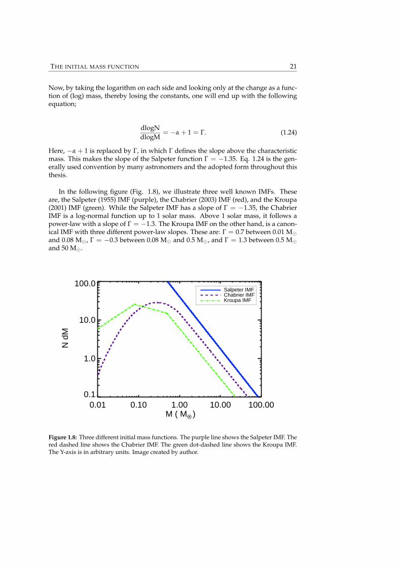
In the following figure (Fig. 1.8), we illustrate three well known IMFs. Theseare, the Salpeter (1955) IMF (purple), the Chabrier (2003) IMF (red), and the Kroupa(2001) IMF (green). While the Salpeter IMF has a slope of Γ = −1.35, the ChabrierIMF is a log-normal function up to 1 solar mass. Above 1 solar mass, it follows apower-law with a slope of Γ = −1.3. The Kroupa IMF on the other hand, is a canon-ical IMF with three different power-law slopes. These are: Γ = 0.7 between 0.01 M¯and 0.08 M¯, Γ = −0.3 between 0.08 M¯ and 0.5 M¯, and Γ = 1.3 between 0.5 M¯and 50 M¯.

0.01 0.10 1.00 10.00 100.00 M ( M

O • )

0.1

1.0

10.0

100.0

N d

M

Salpeter IMFChabrier IMFKroupa IMF

Figure 1.8: Three different initial mass functions. The purple line shows the Salpeter IMF. Thered dashed line shows the Chabrier IMF. The green dot-dashed line shows the Kroupa IMF.The Y-axis is in arbitrary units. Image created by author.

22 CHAPTER 1: INTRODUCTION

The initial mass function offers the great benefit of predicting the likelyhood ofstellar masses at the time of their formation. It has become an important diagnostictool and is of fundamental importance for many astronomical fields. The IMF is usedin areas, such as, galaxy formation and evolution, studies of chemical enrichment,the prediction of brown dwarfs, energetic feedback into the ISM, and in just aboutanything that studies large quantities of stars (Zoccali et al. 2000; Kroupa 2002; Bon-nell et al. 2007). It is therefore appropriate to state that one of the main goals for atheory of star formation is to understand the origin of the stellar initial mass function.

It has been theorized that this distribution is universal in nature, nicely followinga Salpeter slope (Salpeter 1955). Numerous observations of the solar neighbourhoodsupport this hypothesis (Chabrier 2003; Sabbi et al. 2007; Elmegreen et al. 2008) andhas gained a lot of interest since this idea first arose. The shape of the distributionhas been further refined by other astronomers, especially improving upon the lowermass end of the function (Miller & Scalo 1979; Kroupa 2001; Chabrier 2003). A uni-versal IMF would be quite useful, as one can imagine, since it would eliminate onemajor uncertainty in a lot of astronomical fields.

As charming as the idea is, the story does not end there. Several recent studies,of mainly extragalactic objects, have started to show us the other side of the story.At the turn of the century, astronomers were beginning to notice deviations in theirmass functions from a standard Salpeter shape (Baugh et al. 2005; Nayakshin et al.2007; Parra et al. 2007; Dave 2008; Wilkins et al. 2008; van Dokkum 2008; Elmegreen2009). These came from measurements of abundance patterns in extragalactic bulges(Ballero et al. 2007, 2008), enhancement of far infra-red luminosities in interactinggalaxy systems (Brassington et al. 2007), mass-to-light ratios of ultra-compact dwarfgalaxies (Dabringhausen et al. 2009a), NaI and FeH band spectra in luminous ellip-tical galaxies (van Dokkum & Conroy 2010, 2011), and many others. Our Galaxycenter also shows signs of variations in the IMF (Figer 2005a,b; Paumard et al. 2006;Espinoza et al. 2009; Elmegreen 2009; Bartko et al. 2010). Complementary to theseobservations, many numerical studies support a non-universal IMF as well (Klessenet al. 2007; Hsu et al. 2010; Krumholz et al. 2010; Girichidis et al. 2011). Yet, theywere much debated and solid evidence is still lacking. These developments in thelast decade have driven astronomers towards a crossroads, and has divided them,which was the beginning of the IMF’s universality conundrum.

Do all star forming events give rise to the same distribution of stellar masses? Isstar formation essentially a self-regulating process or is fragmentation the processby which stellar masses are fixed? Certainly, the details of either process dependon the physical conditions of the cloud of gas and dust from which the stars form.The unanswered question is: how sensitively does the distribution of stellar massesdepend on the initial conditions in the natal environment? Our ultimate goal is tounderstand the physical mechanisms that are responsible for the origin of stellarmasses.

EXTREME ENVIRONMENTS 23

1.5 Extreme environmentsThe process of star formation is poorly understood in extreme environments. It isuncertain if stars form in the same way everywhere and if the IMF is similar to ourGalaxy or that star formation is severely affected by the harsh, non-Milky Way am-bient conditions. Our Universe harbors many regions which are quite extreme. Anextreme environment in space exhibits conditions that are challenging to the forma-tion of stars. These may include high temperatures, high pressures, strong radiationfields, powerful turbulence, strong gravity, or very low metallicities. Studying theevolution of gaseous clouds and star formation in extreme environments will helpus understand the processes of star formation by determining its limits.

1.5.1 Active galactic nuclei

Active galaxies harbor supermassive black holes with masses of & 106 M¯ in theircenters. Active galactic nuclei (AGN) are the most luminous sources of electromag-netic radiation in the Universe. These accrete matter from the inner parsecs of galac-tic centers. Accretion rates can go up to their Eddington limit, if magnetic fields arenot significant, but are typically ∼10% of this limit (Meijerink et al. 2007). It is alsopossible to surpass this limit in certain circumstances which might play an impor-tant role in the gas accretion process in host galaxies (Kawakatu & Ohsuga 2011).The Eddington rate is obtained when the hydrostatic equilibrium equation, as givenin Eq. 1.15, is set equal to the continuum outward radiation pressure

dPraddr

= −κρ

cFrad = − σTρ

mpcL

4πr2 , (1.25)

where σT = 6.65× 10−25 cm2 is the Thomson scattering cross section for the electronand the gas is assumed to be purely made of ionized hydrogen, κ is the opacitycoefficient of the stellar material, Frad is the radiation flux, L is the luminosity, c islight speed, and mp is the proton mass. The Eddington luminosity then becomes

LEdd =4πGMmpc

σTerg s−1, (1.26)

while the accretion rate can be written as

M =dMdt

=2LEdd

c2 =8πGMmp

cσTg s−1. (1.27)

The matter around black holes is heated up through the accretion process to mil-lions of degrees. This heating leads to the emission of highly energetic radiation,such as UV photons (E > 5 eV) and X-rays (E > 1 keV). The accretion disks shine sobrightly that they are visible from great distances, which renders them easy to spotwith telescopes. Besides strong radiation fields, supermassive black holes impart astrong gravitational field as well. Molecular clouds in the inner 10 pc of active galax-ies will be strongly affected by this gravitational pull as well as the irradiation byX-rays and UV (Meijerink et al. 2007; Hocuk & Spaans 2010a).

24 CHAPTER 1: INTRODUCTION

1.5.2 Starbursts

Starbursts are regions of space with an unusually high rate of star formation. Starformation rates (SFR) are observed as high as several hundreds to thousand solarmasses per year and on the scales of a Galaxy (Sanders & Mirabel 1996; Smail et al.1997; Hughes et al. 1998; Genzel et al. 1998). Massive stars are thought to commonlyform in these places and an exceptional amount of UV radiation (E = 5− 100 eV) canbe seen. The output of UV radiation is dominated by the O and B stars as only thehottest stars produce them. The supernova rate is also generally high in starburstinggalaxies. This will in turn lead to an enhanced cosmic ray rate, since cosmic rays arethought to be produced mainly in supernova remnants (Papadopoulos et al. 2011).Figure 1.9 shows the famous starburst ‘Antennae Galaxies’.

Figure 1.9: The Antennae Galaxies are an example of a very high starburst galaxy occurringfrom the collision of NGC 4038/NGC 4039. Credit: NASA/ESA

Over the years, mounting empirical evidence has been found that there is a cor-relation between nuclear activity and star formation over a wide range of redshifts(Kennicutt 1998; Trichas et al. 2009; Wild et al. 2010). It is thought that there is atight relation between starbursts and AGN (Taniguchi 2004). However, it is still amatter of debate whether the AGN activity is triggering and causing the starburstsor that the AGN is being fuelled by these massive star forming regions. One thingis certain; there is a growing number of galaxies from different samples that exhibitsimultaneous starburst and AGN activity. If there is a causal relation between them,then the question is with which trend. The evolution of supermassive black holes,AGN feeding and feedback to the interstellar medium, as well as the role played bythe environment for the formation of stars, are all relevant issues in the physics ofstarbursts.

EXTREME ENVIRONMENTS 25

1.5.3 Feedback: radiative and mechanical

Accreting black holes and massive stars in dense stellar populations produce a largeamount of energy. During their active episodes they can emit radiation, produceshock waves, and chemically enrich their surroundings. A lot of this energy is de-posited back into the environment from where it was generated. Feedback is a phe-nomenon where the energy that is created within a system, is fed back into the sys-tem itself, altering the ambient conditions and, thereby, influencing the occurrencesof the same phenomenon in the present or future. Two types of feedback, radiativeand mechanical, are very important in active galaxies during the evolution of starforming clouds. Each type of feedback can have positive or negative influences onstar formation.

Radiative feedback will strongly dominate in the form of X-rays, UV, or cosmicrays. Lower energy radiation, like optical or infrared, despite having a strong pres-ence, will be less important in the thermal balance and the chemistry of an interstel-lar cloud. This is because of their lower energies and their increased attenuation in adusty and cloudy environment, although this does add a bit to dust heating. Radia-tive feedback will primarily heat the system as energy is injected into it. However,even then, it is possible to find new ways to enhance cooling. Radiation with highenergies E ≥ 1 keV, like X-rays, will ionize atoms. Ions are much more reactive thanneutral atoms and can easily form molecules with other elements. As such, new andmore molecules will form, helping the system to cool. On the other hand, radiationwith lower energies E ∼ 5− 100 eV, i.e., UV, is more destructive to molecules be-cause of large photo-dissociation cross sections.

The strongest X-rays are produced in accretion disks of black holes. A 107 solarmass black hole accreting at 100% Eddington is able to produce a flux of 100 ergs−1 cm−2 at a distance of 100 pc (Meijerink et al. 2007). X-rays can dominate thethermal balance in AGN upto column densities of 1024 cm−2 and distances of 300pc (Schleicher et al. 2010b). These regions are known as X-ray dominated regions(XDRs, Lepp & Dalgarno 1996; Maloney et al. 1996), and heating is dominated byphoto-ionization. UV radiation has a much smaller penetration depth, which cango upto column densities of 1022 cm−2 (Meijerink & Spaans 2005), at solar metallic-ity. Therefore, it is most effective if the radiation source is nearby. So UV radiationmainly dominates the chemistry of cloud surfaces. UV radiation heats the gas upto a few thousand K through photo-electric emission from (small) dust grains. Theregions where UV radiation dominates, are called photon dominated regions (PDRs,Hollenbach & Tielens 1999). Cosmic rays are not a form of electromagnetic radia-tion. They are rather energetic charged subatomic particles, mostly protons, movingat relativistic speeds. Cosmic rays can pierce through very large columns of gas andtransfer their energy through collisions. Their effect is more subtle and they heat thegas in a molecular cloud almost uniformally. As such, they set the minimum attain-able temperature in these systems (Goldsmith & Langer 1978; Bergin & Tafalla 2007).

26 CHAPTER 1: INTRODUCTION

Mechanical feedback can come from shock waves as well as a strong gravitationalpotential of a nearby black hole or the deep potential wells in starbursts. Gravita-tional stresses produce shearing motions that enhance the turbulence of a nearbycloud if it does not tear it apart. This also has major consequences for the accretionrates of proto-stars. Proto-stars in deep potential wells are able to accrete more ma-terial than their neighbours (Bonnell et al. 2001; Clark et al. 2008a). A contracting,fragmenting molecular cloud, with massive stars in its vicinity, may enjoy strongshock waves as massive stars go supernova. Shock waves can either compress acloud and trigger collapse or blow material away.

Nuclei of active galaxies, e.g., ULIRGs like Arp 220 and Markarian 231, enjoythese extreme conditions, see van der Werf et al. (2010). Strong feedback effects thustake place there, but are difficult to observe directly. Little is known on the IMF inactive galaxies, so theory and simulations are needed to guide our understanding.

1.6 Numerical simulationsSimulation and modelling is an integral part of scientific study. Numerical simula-tions are a powerful tool that can help to better understand the behaviour of pro-cesses. The need for numerical simulations arises when one is limited in performinga study by conventional means, like through analytical work.

In recent years, a large number of studies have been performed on the forma-tion of stars using numerical simulations (Abel et al. 2000; Omukai & Palla 2001;Klessen 2001; Klessen et al. 2005a, 2007; Bonnell & Rice 2008; Wada 2008; Wada et al.2009; Bate 2010; Hsu et al. 2010; Krumholz et al. 2010; Girichidis et al. 2011; Perez-Beaupuits et al. 2011; Clark et al. 2011; Latif et al. 2011; Aykutalp & Spaans 2011a).All these studies address a different aspect in the field or improve on an earlier study.The latter can be done through either adding new physics, more resolution and pre-cision, or by implementing a greater dynamical range.

1.6.1 Grid codes

Grid based codes are Eulerian codes where one follows the fluid in the lab-frame.The grid is divided into the requested number of cells and the maximum resolutionis based on the smallest cell size. The AMR method is a technique which refines thegrid only in the regions of interest, according to a predefined refinement criterion, tominimize computational demand while keeping the resolution high. In this way, onecan achieve very high resolution at any required location. One of the major draw-backs of AMR codes is its diffusive nature. Especially when advecting over largenumbers of grid cells, numerical diffusion is unavoidable. Higher order interpola-tion schemes reduce the effect, but the issue remains. The only way to minimize thisis to increase resolution. On the other hand, a great strength of grid codes is thatthey can handle shocks and contact discontinuities very well.

THESIS OUTLINE 27

Eulerian codes repetitively solve the mass (continuity), the momentum, and theenergy equation. In differential form, these equations, coupled with the Poissonequation for gravity, are given by

∂ρ

∂t+∇ · (ρv) = 0 (1.28)

∂ρv∂t

+∇ · (ρvv) +∇P = ρg (1.29)

∂E∂t

+∇ · (v(E + P)) = ρv · g, (1.30)

where E is

E =12

ρv2 + ρεint, (1.31)

and the Poisson equation is defined as

∇2φ = 4πGρ ⇒ g = −∇φ. (1.32)

In these equations, ρ is the fluid (mass) density, v is the fluid velocity, P is the pres-sure, φ is the gravitational potential, εint is the internal energy per unit mass, and gis the gravitational acceleration.

There is a great diversity of simulation codes available within the astronomicalcommunity. Ranging from very specific codes created just to serve the purpose ofthe author to huge, general purpose numerical codes written by groups of people.FLASH, a grid code designed by Fryxell et al. (2000); Dubey et al. (2009), is an ex-ample of a large scale, multiphysics simulation code with a wide international userbase. The FLASH code forms the basis of the research done in this thesis and isextended with additional physics in each of the chapters.

1.7 Thesis outlineThe theory of star formation is an interesting, illustrious subject with a lot of dis-coveries still ahead. In this thesis, the effects of environmental influences on theformation of stars are studied and the results analyzed. The main focus lies on theinitial mass function of stars, specifically the formation of stars in extreme environ-ments. Each chapter focuses on a different aspect of star formation and each tells itsown tale.

Chapter 2:In the second chapter of this thesis, I focus on the evolution of a giant, r = 10 pc,molecular cloud in a metal-deficient environment. I investigate how metallicity (Z)and an initial rotational moment (β) affects the fragmentation of this molecular cloudinto smaller, but denser, pre-stellar cores. The dependence of molecular cloud frag-mentation is tested on the ambient conditions as they pertain to starburst and dwarfgalaxy regions, which are then compared against the well known conditions of the

28 CHAPTER 1: INTRODUCTION

Milky Way. To properly treat the thermal balance, I use a cooling function, createdby Meijerink & Spaans (2005), that strongly depends on metallicity. The effects ofdust and cosmic rays are also included in the calculations. I simulate the collapsingcloud with these cooling functions for four different metallicities Z/Z¯ = 1, 10−1,10−2, 10−3 and for each metallicity condition I consider five rotational energies, i.e.,β = 10−1, 10−2, 10−3, 10−4, 0, where β is the initial ratio of rotational to gravitationalenergy.

Chapter 3:In the third chapter of this thesis, I study a smaller, r = 0.33 pc, turbulent molecularcore which exists in the vicinity, at d = 10 pc, of an active black hole. I investigate theeffects when this cloud core is irradiated by X-rays, with a flux of 160 erg s−1 cm−2,emanating from the accretion disk of the black hole. The main question of this exer-cise is whether star formation is significantly affected by hard X-rays. I perform a fullradiative transfer calculation to obtain the proper temperatures inside the molecularcloud by using an XDR code (Meijerink & Spaans 2005). In this study, my focus lieson the emerging IMF in an X-ray dominated region and I assess whether it deviatesfrom a Salpeter shape.

Chapter 4:In the fourth chapter of this thesis, I continue my work on molecular cores in AGN.This chapter directly follows the previous chapter but expands the study on the feed-back effects in extreme environments. I now also incorporate the effects of gravita-tional shear (mechanical feedback), cosmic rays, UV, and varying X-ray fluxes (radia-tive feedback). A parameter study of 42 different 3D hydrodynamical simulations isperformed in order to capture the qualitative and the quantitative effects that the en-vironment imparts on interstellar clouds inside active galaxies. I look at the changein the equation of state and its role in the dynamics of the cloud core. I also analyzehow the phase-diagrams, the star formation efficiencies, and the initial mass func-tions are influenced in active galactic environments.

Chapter 5:In the fifth chapter of this thesis, I combine the results of the previous chapters andevaluate them from a general perspective. I summarize my main findings and givemy best answer to the principal question of this work: what is the IMF in activegalactic environments? I take the opportunity to discuss what other research pathscan be taken to study the origin of, and variations in, the IMF, specifically the role ofmagnetic fields.