University of Groningen

Grid-size reduction in flow calculations on infinite domains by higher-order far-fieldasymptotics in numerical boundary conditionsWubs, Friederik; Boerstoel, J.W.

Published in:Journal of Engineering Mathematics

IMPORTANT NOTE: You are advised to consult the publisher's version (publisher's PDF) if you wish to cite fromit. Please check the document version below.

Document VersionPublisher's PDF, also known as Version of record

Publication date:1984

Link to publication in University of Groningen/UMCG research database

Citation for published version (APA):Wubs, F. W., & Boerstoel, J. W. (1984). Grid-size reduction in flow calculations on infinite domains byhigher-order far-field asymptotics in numerical boundary conditions. Journal of Engineering Mathematics.

CopyrightOther than for strictly personal use, it is not permitted to download or to forward/distribute the text or part of it without the consent of theauthor(s) and/or copyright holder(s), unless the work is under an open content license (like Creative Commons).

Take-down policyIf you believe that this document breaches copyright please contact us providing details, and we will remove access to the work immediatelyand investigate your claim.

Downloaded from the University of Groningen/UMCG research database (Pure): http://www.rug.nl/research/portal. For technical reasons thenumber of authors shown on this cover page is limited to 10 maximum.

Download date: 10-02-2018

Journal of Engineering Mathematics 18 (1984) 157-177 © 1984 Martinus Nijhoff Publishers, The Hague. Printed in The Netherlands

Grid-size reduction in flow calculations on infinite domains by higher-order far-field asymptotics in numerical boundary conditions *

F.W. WUBS **, J.W. BOERSTOEL and A.J. VAN D E R WEES

National Aerospace Laboratory NLR, P.O. Box 90502, Amsterdam, The Netherlands

(Received July 7, 1983)

Summary

An error analysis is presented of the numerical calculation of the steady flow on an infinite domain around a given airfoil by a domain-splitting (= zonal) method. This method combines a fully-conservative finite-dif- ference approximation on a finite domain around the airfoil with an approximate asymptotic solution outside this finite domain. The errors are analyzed as a function of the accuracy of the approximate asymptotic expansion, of the distance to the airfoil of the far-field boundary of the finite domain and of the mesh size. The numerical experiments show that, for a given desired accuracy level, large reduction in grid sizes are possible, if the usual far-field asymptotic approximation (uniform flow plus first-order perturbation by a circulation vortex at infinity) is augmented by only a few extra terms in the approximate asymptotic far-field solution. In this way, considerable numerical efficiency improvements can be realized. It is expected that this conclusion can be generalized to many other applications where computations on infinite domains are performed.

1. Introduction

In computa t ional fluid dynamics problems on infinite domains, where the far-field flow is

a small per turba t ion of an inviscid uni form parallel flow, the infini te size of the flow

domain can be handled by what nowadays is called domain-spl i t t ing [2] or zonal method

[3]. The numerical calculations are then restricted to a finite inner domain, while outside

this inner domain a simple model of the flow is used. Examples are aerodynamic

calculat ions of steady compressible subsonic or t ransonic flows a round aircraft or airfoils by finite-difference methods. The finite-difference calculations are restricted to a large but

finite " i n n e r " computa t ional domain, while on the corresponding "outer" domain the flow is assumed to be a steady uni form parallel flow, or a small per turba t ion of such a

flow in which nonl inear compressibil i ty effects and aircraft or airfoil thickness effects are

neglected. In order to obta in a well-posed finite-difference problem on the finite inner domain, a suitable numerical boundary condi t ion on the far-field bounda ry can be formulated from this assumption.

* Exploratory research study of the National Aerospace Laboratory NLR, Amsterdam, The Netherlands, ordernumber 554.203, workplan 1982 3.5,C.6. The results of the study have been reported in a doctoral script of the first author, presented at the University of Technology, Twente, The Netherlands [1]. The authors are indebted to Prof. dr. ir. P.J. Zandbergen and prof. dr. ir. C.R. Traas for their contributions and stimulation.

** Currently at Mathematical Centre, Kruislaan 413, Amsterdam, The Netherlands.

157

158

! l i~ , . , ,#; ...'..." " v. " ,~%S , m - k m ~

• I h l = : . o :/ ~. ,..oo=lNm mlmm.=-, : :: . - o = m l m l l l l l l l

IIIIIinm~=-'~. ::~ - - : : : : = ; . . i i i n l l l l l l l

:i)ii;,~i N?il="gN

IW,4~=~,~=t,$=ll~=gli.*~lllllllllli,=;tt~.~tl*=tl'=t~=i~l

[~ ~ SHOCK WAVE

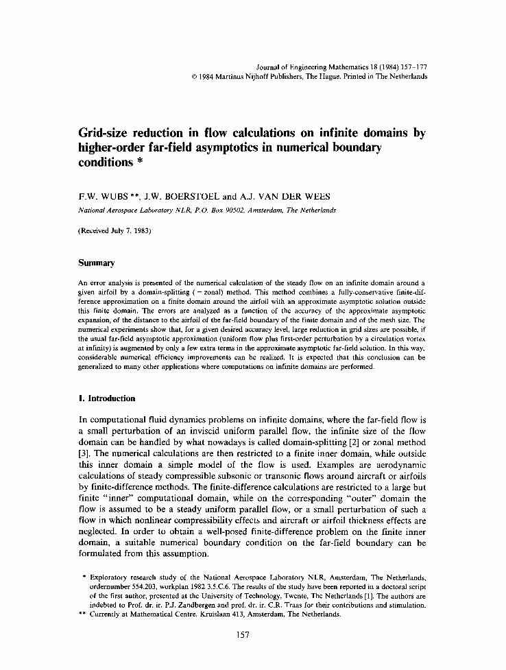
Figure la. Far-field part of 130 × 42 grid around N A C A 0012 airfoil.

Figure lb. Lines of constant Mach numbers in computed transonic flow around N A C A 0012 airfoil ( M ~ = 0.75, a = 2°).

130 GRID LINES, UNIFORMLY DISTRIBUTED ~ 1

- - AIRFOIL IMAGE

,?

. . . . . IMAGE OF FAR BOUNDARY OF GRID

OUTER 400/o

OF GRID

'V

Figure lc. Lines of constant speed on uniform computational grid in computed transonic flow around N A C A 0012 airfoil (MoQ = 0.75, a = 2°).

159

There are various reasons to investigate whether this technique can be improved by using more accurate solutions of the flow equations on the infinite domain. • Recently it has become clear that, on large parts of grids in calculations of transonic flows around airfoils, the velocity is a smooth function of the grid coordinates. A typical example from current engineering practice is presented in Fig. 1 [4]. On about 40% of the grid near the far-field boundary, the lines of constant speed show a very smooth and regular pattern around the free-stream speed value 1.0, see Fig. 1.c. It may be expected that such velocity fields can be approximated more efficiently by a small number of appropriately chosen asymptotic solutions of the flow equations at infinity, instead of by a grid function. • In time-dependent flow calculations, recently so-called non-reflecting or weakly reflect- ing numerical boundary conditions have been proposed and applied with great success to prevent nonphysical numerical reflections of outgoing waves at the far-field boundary of inner domains (see e.g. [5-7]). The boundary conditions, which are generalizations of well-known radiation conditions, have the form of differential expressions, allowing only physically-relevant outgoing waves. Similarly, in steady-flow problems differential expres- sions can be used, which allow a more accurate asymptotic expansion as its solution. • A third reason concerns the calculation of drag. Detailed analysis of the calculation of transonic flows around airfoils [4] has shown that reliable calculation of drag is difficult because of a too crude approximation of the flow on the infinite outer domain, causing effects which are known to aerodynamicists as wind-tunnel blockage effects. This situation may be remedied by more accurate solutions on the outer domain.

Summarizing, application of higher-order asymptotic theory seems to promise im- proved numerical approximation efficiency. It should allow the replacement of the approximation of the flow on the outer 40% of a grid by a combination of a small number (5 to 10) of asymptotic solutions on the other domain, leading to grid-size reduction. This grid-size reduction should then give substantial savings in computer runtime, because the total number of unknowns in the computational problem is also reduced by say 40%. Such savings help to bring down the calculation costs of three-dimensional flows around aircraft down to a level where repeated calculations for design purposes become feasible. Moreover, the accuracy of the calculation of drag should improve considerably.

The present study has been undertaken to explore the first of these speculations: the possible grid-size reduction, as a function of the accuracy of far-field solutions, for a fixed error level in the overall numerical simulation. Incompressible flow around lifting airfoils was taken as a test problem. The nonlinearity in computational aerodynamics (due to compressibility) is only a minor additional complication, from the point of view of approximation accuracy, it only complicates the algorithm, and has thus been removed from the model problem.

The study was thus primarily meant to resolve accuracy and approximation questions concerning converged steady flows, and not to design fast and robust solution algorithms, However, in the concluding discussion it will be argued that efficient solution procedure for steady-flow problems may be expected in combination with multigrid techniques.

The material of the study is presented as follows. • Section 2: Test-problem formulation for incompressible flow around lifting airfoil. • Section 3: Discretization of test problem by domain splitting, fully-conservative finite differencing on the inner domain,and construction of asymptotic expansion on the infinite outer domain. Formulation of numerical boundary conditions, and of techniques to determine or eliminate the unknown coefficients in the asymptotic expansion. Outline of solution process.

160

• Section 4: Numerical experiments, test strategy, dependence of error level on domain size, number of terms in asymptotic expansion, and mesh size. • Section 5: Conclusions, and discussion of generalizations.

2. Description of test problem

The test problem is an inviscid, irrotational, and incompressible flow around a lifting airfoil. Introducing a velocity potential, qo, the mass conservation in the flow is governed by Laplace's equation:

Acp = 0. (1)

At the airfoil, the mass-flux is zero:

a___~= a. 0. (2)

At infinity, a uniform parallel flow is assumed, and from the general solution of (1) we then may derive the following expansion for ~p at infinity:

FO ~o = x + ~-~ + O ( r - ' ) . (3)

where F, the circulation, is an unknown scalar, 0 = arctan(y/x), and r 2 = x 2 + y 2 . The angle 0 is not single-valued, and therefore a slit has been made along the positive x-axis, where ¢p makes a jump of magnitude F. The value of F should be chosen such that the velocity remains bounded, especially at the trailing edge of the airfoil (Kutta condition). It can be shown that the above problem is well-posed and has a unique solution for ¢p and F.

3. Numerical discretization and solution process

The problem described in Section 2 has been solved using a domain-splitting (zonal) method. For the discretization, a finite-difference approach has been used. The resulting set of equations has been solved iteratively by successive-line relaxation, accelerated by Richardson extrapolation.

3.1. Domain-splitting

In domain-splitting methods, the physical domain is split in several coupled subdomains, in which different physical models and /o r numerical solution methods are used. In the test problem, a simple split into two domains is introduced (fig. 2); a bounded inner domain A, where a fully-conservative finite-difference method will be applied, and an unbounded outer domain B, where an analytic approximation of the flow will be used. In both domains, Laplace's equation must be satisfied, and the solutions on the two domains must be appropriately coupled at the boundary C - which is assumed to be regular - so that a unique solution is obtained on the entire domain. It can be shown that the continuity of cp and cpn over C is sufficient for continuity of all higher derivatives of cp over

161

n-DIRECTION

C

B

,5¢=0

Figure 2. Splitting into two domains A and B.

C. Three discrete methods of coupling have been investigated; these will be identified as the % cp-method, the % %-method, and the DE-(differential equation) method.

3.1.1. % q~,- and the ~, ~-method On the outer domain B, the solution of (1) will be approximated by a part of the general solution,

F 0 N qo = x + ~ + Y'~ (a . cos nO + b. sin nOlr-". (41

n = ]

Observe that for N < oo this is a finite linear combination of particular solutions of Laplace's equation, with a, , b, free constants to be suitably determined. On the inner domain a finite-difference approximation will be constructed (Section 3.3).

START SOLUTION _1

CONTINUOUS AT C

I OIRICHLET CONDITION AT C I

I

SOLVE ~ IN A

SOLUTION ESTIMATE

INR

SOLUTION ESTIMATE

INA

LEAST-SQUARES FIT TO MINIMIZE ERRORS IN CONTINUITY REQUIREMENTS

\ I CONDITION

FOR ~B

/ I CONDITION

FORe B

CONTINUOUS AT D "Pn CONTINUOUS AT C

Figure 3. Summary of qo, ~,- and tp, ¢p-method.

162

Continuity of cp and % over C can numerically be assured by taking N large enough in (4), i.e. equal to the number of mesh points of the finite-difference approximation on the boundary C. In practice, a certain discretization error in the continuity requirements is acceptable. This freedom will be used to limit the number of terms N in (4) as much as possible. The continuity requirement for ~ or % was chosen to be imposed in a least-squares sense, giving the algorithm of Fig. 3.

The algorithm works as follows: starting with an approximate solution on the outer domain B, the solution is restricted to the boundary C, giving a Dirichlet condition for the inner domain A, where the problem is solved by a finite-difference method. In the % ~n-method, a normal derivative at curve C is now computed from the infinite-difference solution; in the % 9~-method a potential 9~ is computed on a curve D, slightly different from C. This finite-difference representation of cp or ~ is fitted to the ~ or ~n on the outer domain B by a least-squares fit, giving a new approximate solution in B. The ~ or % will be continuous over C only in a least-squares sense.

3.1.2. DE-method In the DE (differential equation) method, the series expansion (4) is replaced by a differential equation, applied along the curve C, and having a number of terms of the expansion as its solution. The expansion (4) may be slightly generalized to

F0 oo ~=x+~- - -~+ E f , (O)r-". (5)

n = l

It can be shown [1] that the DE

B ~ = B. ~ = 0 , B . = O / O r + ( 2 n - 1 ) r -1, (6)

has the first N terms of the sum of (5) as its solution. Therefore, if the DE

is applied to the finite-difference approximation along the curve C, the DE effectively imposes a boundary condition, which has (5) up to term N as its solution.

The DE-method is, in contrast to ~, ~- or e0, %-methods, implicit, i.e. it does not need explicit evaluations of coefficients a , , b~ in (4), and specification of the form of the functions fn(0) in (5). However, it is impractical to handle many terms of (5), as the DE will then be of a high order, and is hard to discretize. The ~, e0- and ~, %-methods have more flexibility in this respect.

3.2. Application of% cp- and ~, %-method to the flow around a circle

To obtain some insight in the convergence of the described iteration algorithm of Fig. 3, the application of this algorithm to the calculation of the steady flow around a circle has been analyzed. The analytic solution is known:

= r cos 0 + r ] cos 0, (8) r

C

B

~ ¢ = 0

Figure 4. The curves C and D, used to couple the solut ions in A and B.

163

where r I is the radius of the circle. This circle-airfoil and the curves C and D (Fig. 4) are assumed to be concentric circles with radius r 1, r E, r 3, respectively (r 1 << r 3 < r E).

The solution of Laplace's equation in the inner domain A may be given the general form:

ep=rcosO+ rS{ c o s 0 + ~ (aocosnO+b. sinnO)r". (9) r

n = - - O O

This approximation has the form of the exact solution plus a perturbation which should be shown to tend to zero. Using the boundary condition O~/Or = 0 at the circle, this approximate solution becomes

q g = r c o s O + r2 cosO+ (a . c o s n 0 + b , s inn0) r " + - - r r n ]"

n=O (a0)

This solution must be coupled with an approximate solution in domain B, which may be written as

N

~ = r c o s O + r--~lz cosO+ ~E] (~. cosnO+ b. sinnO)r-". (11) r

n = l

Here, we have omitted the particular solutions with n < 0, because Vq0 must be bounded for r --, ~ (free-stream boundary condition).

When the continuity requirement in q0 is applied on the curve C, the following relations between coefficients on the inner domain and on the outer domain are obtained:

ao k = O, bo k = 0, (12.a)

a r2 n + 1 ~k - n = a,r 2 , n = 1 . . . . . N, (12.b)

a , = b, = 0 for n > N; (12.c)

(12.b) holds also between b, k and -k b,~. The superscript k has been appended to indicate that the coefficients are those of the k-th iteration of the iteration algorithm of Fig. 3.

164

From Fig. 3 it is seen that in the % %-method the outer solution is further coupled to the inner one by the demand that % is continuous over C. This gives the equation

N /( r Zn) _ _ _ k k _ n r ~ + l cos0 rE COSO+n=I ~ ( a n c ° s n O + b ~ sinnO nr~ -1

r? = cos 0 - r2 cos 0 +

N

y~ ( _-k-~, "k+, ), (13) u n c o s n O + b ~ s i n n O ) ( - n r ~ -1 n = l

where a~ and b~ are defined by (12.b). This gives new relations between the coefficients of inner and outer domain:

r n): k+ln F~+ 1 -- an rl n = 1 . . . . . N, (14)

with the same formula for b~. We are interested in reduction factors of the coefficients after one iteration cycle of the algorithm of Fig. 3. In the case of the ~, %-method, substitution of (12.b) in (14) gives the reduction factors

u~--z---- = (15) -k r 2n r}n , . = , . . . . N. a n +

This formula shows, that the coefficients tend to zero (as desired) in an oscillatory k manner, slowly for r I << r 2. This process can be accelerated by underrelaxation (a~ +1 = an

+ o(a~ +1 - a ~ ) ) . In a straight-forward manner, the relaxation factors

r? n % = ½ + - - n = l . . . . ,N (16)

2r2n '

are found. So o = ½ + r2/ (2r 2) will provide a good relaxation factor for all coefficients, when the % %-method is applied.

The % q0-method differs from the % %-method in the computation of the outer solution from the inner solution. This time, rp should be made continuous on the circle D. This means that the additional continuity relation is resembling equation (12.b), but it should now hold on circle D with radius r 3, i.e.

( k n ~ k + l - n a . r3 + = a n r 3 , n = 1 . . . . . N. (17)

When this is combined with (12), the reduction factors

~k+, 4 " + r?" , , - - 1 . . . . . u (18) -~ ~ . + , - } " '

an

165

are found. This equation shows that the lower-order terms converge slowly. Acceleration is again possible by relaxation, here overrelaxation. The relaxation factor is

r2n + r?n n = 1 . . . . . U. (19) ° . - q ° _ q . ,

An overrelaxation factor for all n may be chosen to be

r22 + r2 (20) O " - - - -

r 2 _ q "

However, this factor should not be so large that it causes higher-order terms to diverge. This is assured if

o < 2. (21)

This restriction results in a slower convergence rate for the % cp-method compared with the % ¢p,-method.

In the case of airfoil calculations, it was found that under- or overrelaxation improved the convergence rate of the iteration processes significantly. The convergence analysis of the section thus seems to be indicative for what has to be done in more general situations.

3.3. Finite-difference approximation

The equation (1) has been discretized on an 0-type grid (Fig. la). In this grid, potentials are given at midpoints of cells, and velocities at midpoints of cell boundaries. Using tensor-calculus, a fully-conservative finite-difference method has been formulated [1]. At the airfoil, virtual points are introduced to achieve second-order accurate approximations of the boundary conditions.

The transformation of an 0-type grid to an equidistant computational grid in a computational rectangle was based on an approximately conformal mapping of an airfoil to a circle producing near-orthogonal grids. The mapping is singular at the trailing edge. It may be shown that this implies that the transformed velocity in the computational rectangle then must be zero at the trailing edge to guarantee finite velocities at the trailing edge. Thus, the Kutta condition has been transformed from a qualitative to a quantitative condition. In the computations, the zero transformed velocity at the trailing edge is accomplished by means of a Newton iteration on the circulation.

3.4. Solution method

The solution method of the finite-difference equations was based on successive line relaxation (SLOR), because for this method the theory is well-developed. The SLOR iteration matrix was derived in the usual way directly from the system matrix of the problem. This gave iteration matrices that were diagonally dominant, except possibly at the boundaries. Here, diagonal dominance is often lost due to central differencing in the discrete boundary conditions. As convergence of SLOR is usually realized by using diagonally-dominant iteration matrices, the iteration matrices were made diagonally

166

dominant at the boundaries, too, by making O(h) modifications to the finite-difference boundary conditions for SLOR solution-corrections. These modifications are more drastic for DE-methods than for % ~,,- and cp, ep-methods - where always a Dirichlet condition at boundary C is used - and have slowed down the convergence of the DE-methods. For details about this non-standard issue, see [1].

The line relaxation has been accelerated by Richardson extrapolation, which will briefly explained here. After a sufficiently large number of SLOR iterations, the following relation approximately holds in practical calculations:

Aqo" + 1 = h A~", Aqo" + l = qo" + 1 _ ¢p,,, (22)

where h is the largest eigenvalue of the SLOR iteration matrix (usually slightly less than unity). If at certain stages of the iteration process, the above relation holds to a sufficient degree, an estimate of the ultimate Acp = q0 ~ - cp" can be based on knowledge of the value of this eigenvalue. We assume the SLOR process to converge with fixed h, so that

Aft,= ~., Acp 4. (23) k = n + l

This relation can, together with (22), be used to define

1 A~v = 1 _--S--~Aq~"+l. (24)

In our numerical calculation, this extrapolation on the largest eigenvalue has been applied when the variance of the last three eigenvalue estimates was below a certain given value. A sample convergence history is shown in Fig. 5. The vertical lines indicate the iterations where the extrapolation is applied. It is clear that the well-known slowdown of the convergence due to the largest eigenvalue of the iteration matrix is remedied by the extrapolation (see e.g. iterations 20, 52). If properly applied, the number of iterations can be reduced by more than a factor of two [8].

to ~l~ DEI-METHO0 NORMAL GRID

Io _~I

10 -

10

I0

I0

IO , , , v I ' ' ' ' I l l

o so ITER too

Figure 5. Convergence history of SLOR combined with Richardson extrapolation.

167

4. Numerical experiments

The objective of the present investigation is the relation between the number of N of terms in the asymptotic far-field solutions (4) or (5) used in the numerical boundary conditions, the size of the computational domain, and the mesh size in the finite-difference approxi- mation. In this respect, we are interested in:

1. The error, when the size of the domain is varied (using a fixed number N of terms in the boundary condition).

2. The error, when the number of N terms of the expansion is varied (on a fixed domain). 3. The comparison of the errors for the DE-, % ep*- and 9~*, 9~,*-methods, both qualita-

tively and quantitatively. 4. The error as a function of the mesh size in the finite-difference calculation.

4.1. Test case

Computations have been done for the von Karman-Trefftz airfoil, for which the solution is analytically known. The results will be presented by means of plots of Ce-errors, which is the difference between the analytical and the numerical pressure coefficient on the airfoil surfaces. A comparison in terms of Cp-errors has been chosen as the pressure distribution on the airfoil is of great practical importance in aerodynamics, and errors tend to be largest on the airfoil surface. The angle of attack of the airfoil is 4 degrees. The Cp-distribution of this case (Fig. 6) has a form representative for engineering applications. The circulation F is a direct measure of the amount of lift on the airfoil.

Four differently-sized grid domains have been studied, and on each domain, seven different boundary conditions have been imposed at the outer artificial boundary. These conditions were formed from the basic three methods (% q~-, ~, %,-, and DE-method) by varying the number of terms N, giving 9~9~0-, epqp2-, ~99 2-, 999~5-, 9~%5-, DE1-, DE2-meth- ods, where the sequence number indicates how many terms of the expansion have been used.

The sizes of the grids, corresponding to the domains 1 through 4, are respectively 64 × 18, 64 × 14, 64 × 10 and 64 × 8 points. Some computations have been performed on domain 3 and 4 on fine grids, containing 128 × 18 and 128 × 14 points, to assess the influence of the mesh size. From preliminary experiments, it was concluded that these

2

Cp

- - 1

l J I |

1

] l i l t

- - 2 0

Figure 6. Analytical Ce-distribution. Von Karman-Trefftz airfoil, a = 4 °, F = 0.92918.

168

" / /

Figure 7a. Normal grid.

Figure 7b. Enlargement of fine grid at leading edge. Figure 7c. Enlargement of fine grid at trailing edge.

values of N will give a good insight in the possibilities of grid-reduction through extra terms of the asymptotic expansion. The graphs of the grids on the four domains are shown in Fig. 7, together with enlargements at leading and trailing edges.

For the purpose of this article, the results of the qoq~0-method on domain 1 are considered to have an acceptable average-standard-error level. This numerical error level represents an often accepted standard of error level in aerodynamic calculations. This will be used to judge the accuracy quality of the various results in terms of better or worse than the standard-error level.

4.2. Results

The results are presented in graphs and tables. Each page shows the seven methods on one domain. The pressure-coefficient error (C e exact -C e computed) is indicated in the plots by CPE-CPC. The arclength along the airfoil is denoted by s, starts at the trailing edge on

169

the upper side and ends at the trailing edge on the lower side. In all graphs, the values CPE-CPC= +0.02 are indicated by two horizontal lines. Ideally, CPE-CPC curves should be at least between these two horizontal lines, because computational results not

002

CPE - CPC

0,00-

-0.02 -

- 0 . 0 4 -

-0 .06 o ~

~,pOMETHOD S

METHOD U

exact .9291808

uo0 .917 uo2 .932 uun2 .932 ~o5 .932 Uen5 .932 DEI .931 DE2 .932

0.02

CPE - CPC

T 0.01

000

- 0 0 1 -

-0.02

F Lp.o2 METHOD

0.02 -

CPE - CPC

0.01

0.00

- 0 0 1 -

l 0 0 2 -

6 8 0

S

1 ~o~on2 METHOD - - - ~ S

002

CPE - CPC

T 001

0.00

-0.01

--002

0.02 -

CPE - CPC

T OD1,

0 . 00

- 0 . 0 1 ,

-0.02

- 7 ]

4

~ 0 5 METHOD

I 6

2 4 6

DE1 METHOD - ~.

0.02

CPE - CPC

0.01

0.00

- 0 . 0 1 -

-0 .02

0.02 -

qO4~n 5 METHOD

CPE CPC

0.01

0.00

-0.01

0.02 2 ~ ~

DE2 METHOD

F i g u r e 8a. Cp error resu l t s for: a = 4 ° , d o m a i n 1, M = 65, N = 17.

170

0.05 -

CPE - CPC

T - 0.00-

- 0 , 0 5 -

~ 0 1 0 -

- 0 1 5 -

0 .20- 0

0.0 ' !

CPE - CPC

T 0.01-

0 . 0 0 .

-0 .01 -

0 . 0 2

0 0 2

C P E - CPC

T 0.01.

0 . 0 0 .

- 0 , 0 1 ,

- 0 . 0 2

0 .02

CPE - CPC

0.01

0.00

-0 .01

- 0 . 0 2

- ~ r r r r

Kotp0 METHOD

METHOD U

exact .92918

~eO .883 oe2 .931 e~n2 .930 ee5 .932 ~ n 5 .932 DE1 .928 DE2 .932

~tp2 METHOD ~ S

~4~5 M E T H O D ~ S

DEI METHOD

0.02

CPE CPC

T 0.01

0.00

: 0 0 1 -

- 0 , 0 2

~tOn2 M E T H O D

0.02

CPE - CPC

0.01

0.00

- 0 . 0 1 -

- 0 0 2 -

1 q:Wn 5 METHOD

0 . 0 2 . . . . . . . .

CPE CPC

? 0.01

o o o

-0 .Q i

- 0 . 0 2 2 4 6

DE2 METHOD

Figure 8b. Cp error results for: a = 4 °, domain 2, M = 65, N = 13.

sa t i s fy ing this cri terion m a y be c o n s i d e r e d to be too inaccurate for eng ineer ing appl ica-

t ions. F igure 8 s h o w s 28 p lots o f the pressure-coe f f i c i ent error C P E - C P C versus s, as a

171

0 3 ~

04

06

O6 o 2 ~

~ 0 METHOD ----t.

M E T H O D F

exact . 92918

oeo .803 t.)o2 . 9 1 7

c,',,) n 2 . 9 0 2

o~,~5 .933 ,-,,~,n5 .933 DE1 . 8 9 9

DE2 .931 iii i

0.02 -

(,PE CPC " 0.00

002"

-004•

006-

- 008-

0.10 0

\

~L02 METHOD

005

CPE CPC

I - 0 o n ,

005,

0102

0152

-020 ~ ,~ ,~ 8

W.on2 METHOD ~ S

002 --

CPE CPC

T 0.01

CPE

T

000

001

0.02

"m

0 2 ~. 6 q1#5 IVlE] HOD

0.02

CPC

001

000

-001

-0.02 0 2 4 6 8

DE1 METHOD - - ~ S

002 " ' CPE CPC

t 001

0.00

-0 01

-002 0

0 02 ....

001 1

000

0

qt

, - - ~ ~ ~ - ' ~ - - ~ - -

~.On5 METHOD .

function of the four domain sizes and the seven far-field boundary-condit ion discretiza- tions. Every figure also shows a table of calculated circulation values F. From all graphs it may be seen that the greatest errors occur at the trailing edge and at the leading edge of

Figure 8c. Cp error results for: a = 4 °, domain 3, M = 65, N = 9. DE2METHOO

172

0.2

C P E - CPC

T 0 . 0

- 0 . 2 -

- 0 . 4 -

- 0 . 6 -

- 0 . 8 -

- 1 . 0

q:~.PO METHOD ~ S

METHOD F

exact .92918

e~o0 •723 0o2 .890 oon2 .847 ~o5 .939 O(9nS .932 DE1 .849 DE2 •925

0.1

CPE - CPC

" 0 . 0

- 0 . 1

- 0 . 2

- 0 . 3

0 .4 . ' ~ , ~ , ~ .

tp, p2 METHOD

0 . 1 -

CPE - CPC : ~r 0 .02

] - 0 . 1 ~

- 0 , 2 .

- 0 . 3 .

- 0 . 4 .

- 0 . 5 .

-0 ,6 " 2 4 6 8

q:kOn2 METHOD -----I. S

0.02 -

CPE - CPC

T 0.00.

- 0 . 0 2 -

-0.04.

- 0 . 0 6 .

- 0 . 0 8 .

xlO -= 0.75

4 6

Lp, p5 METHOD

CPE - CPC :

050-

0.25 -

-0.00-

-0.25-

- 0 . 5 0 -

- 0 . 7 5 o ~

DE1 METHOD

0.05.

CPE - CPC

-0.00,

-0.05-

-0 .10.

- 0 . 1 5 -

0.03 -

I , I , 6 8

qXPn5 METHOD ~ S

CPE - CPC

~" 0.02

0.01 -

o.oo.

-0 .01 -

-0.02 0 2 4 6

D E 2 M E T H O D

F i g u r e 8d . Cp error re su l t s for: a = 4 ° , d o m a i n , 4 , M = 65 , N = 7.

the airfoil. The first error is a result of the singularity of the transformation at the trailing edge (see Section 3.2). This error is not of O(h2). The error at the leading edge is due to strong gradients. This error reduces well with grid refinement.

173

Figure 8a (artificial boundary at about 2½ chords (= airfoil-lengths) distance, Fig. 7a) shows that the Cp-error can be reduced to an acceptable engineering level by only one term (DEl-method). Because all graphs, except ¢pcp0, are identical we can conclude that the error in these results of Fig. 8a is mainly caused by the mesh width, and that second- and higher-order terms in the asymptotic expansion are not significant, when the boundary is this far away. Notice also that the calculated circulation values are about an order of magnitude more accurate than those of the standard ¢pcp0-method. Figure 8b (artificial boundary at about 1½ chords distance) shows that the cp~p0-method results have become considerably worse (compare with ¢pcp0 in Fig. 8a.) The other results are still excellent, and the error is an order of magnitude smaller than those of the cpcp0-method. Figure 8c (artificial boundary at about 1 chord distance) shows that also the accuracy of the ¢prp2-, qvcp,2- and DEl-method becomes considerably worse. Apparently, on a domain of this size, the higher-order terms in the asymptotic far-field expansion are going to play a role. Figure 8d (artificial boundary at about 3 /4 chord distance) shows, that only the results of the ¢pcp5-, and DE2-method are still acceptable.

It is remarkable, that the DE1- and DE2-method give better results compared with the tp, cp- and ¢p, ¢p,-method, for the same number of terms used in the expansion. This is probably due to the fact that the DEn-operator allows a more general solution, because it does not prescribe the precise form of the functions of O (compare (4) and (5)), so the ¢p, ¢p- and ¢p, ¢p,-method use a smaller class of functions and will in general require more terms to obtain a given accuracy.

4. 3. Some results on the f ine grid

From the results of Fig. 8a it follows that, for all methods, except the tpcp0-method, the error level is dominated by the mesh size, and not by the number of terms in the far-field expansion of cp. Hence, it seems appropriate to check this by investigating the effect of mesh-size halving. Not all experiments need to be repeated on a fine grid, because sufficient information may be obtained from a selection. Here, the calculations with the cptp2-, cpcp,2-, ¢pcp5-, tpcp,5-, DE1- and DE2-method are reported on the fine grid on domain 3 (128 x 18 points), and the cpcp5- and ¢pcpn5-method also on the fine grid on domain 4 (128 x 14 points).

The error graphs are presented in Fig. 9a-9b. From these figures, it may be seen that there are two dominant errors. The first one is caused by the truncation of the expansion on a fixed domain. The second is the numerical error caused by the mesh size. The first error can be seen clearly by comparing, on domain 3, ¢pcp2, ¢ptp,2, DE1 in Fig. 8c to Fig. 9a. There is no significant altering of the Cp-error so two terms are too few on this domain. On domain 4, the same is true for ¢pcp5 and ¢p9~,5, see Fig. 8d and Fig. 9b. The second error, caused by the mesh width, is dominant in the results for the ¢p9~5- and ¢pcp,5-method on domain 3 (Fig. 8c and Fig. 9a). It depends thus on the importance of the latter error whether better results can be achieved on a final grid. The DE2-method in Fig. 8c and Fig. 9a shows a case, where both error have about the same importance.

Note that the error in the circulation value is not directly determining the overall accuracy of the method. For instance, in Fig. 8d we find for the ¢p%5-method a good value for F, but the Cp-error graph of ~pep,5 is worse than the error graph of epcp5.

4.4. Remarks concerning convergence rates

Concerning numerical convergence aspects, the following conclusions were arrived at. For details, see [1].

174

• A grid-s ize reduct ion was usual ly a c c o m p a n i e d by a propor t iona l decrease in c o m p u t a - t ion t ime, w h i c h m e a n s that the m o r e c o m p l i c a t e d far-f ie ld a p p r o x i m a t i o n m e t h o d s do

not give a substant ia l overhead.

METHOD ["

exam .92918

ou2 .915

e~n2 .898 ee5 .931 ~ n 5 .932 DE1 .901 DE2 .930

0.02 CPE CPC "

' 0 . 00 -

-0.02"

-004-

-0.06-

-0 .08-

-0.10 0

q;W2 METHOD

O.05- CPE CPC

" -0.00

005-

014

01

021

\

- - ~ , ,~ ' ' - -

~Pn2 METHOD

002

CPE CPC

T 0.01

0 O0

-0.01

-0.0~ ~ ~ ' 8

tc~p5 METHOD ~ S

002

CPE i, CPC ~

001 "1

0.00 I '¢'-

0.011 " ~

0.02 , -I~ - , o 2

WPn5 METHOD

8 ~ S

CPE - ? 0021 CPC

0.01

o oo , 1 ' . . . .

o.o o ~ ~ ' ~ '

DE1 METHOD

002- CPE CPC

T 0 ,01 -

0.00

001.

0 02.

DE2 METHOD

Figure 9a. Cp error results on fine grid, a = 4 °, domain 3, M = 129, N = 17.

0.02 --

CPE CPC

T 0.00 -

0.02-

- - 0 . 0 4 -

0 . 0 8 -

175

METHOD I"

exact .92918

ee5 .939 ~en5 .933

q:~95 METHOD

6

0 0 5

CPE CPE

t - 0 ~

0.0

010-

0.15

7 - 5

. . . . . . . . . . . . . . .

6 qoko n 5 METHOD

Figu re 9b. Cp e r ro r resul ts o n fine grid, a = 4 °, d o m a i n 4, M = 129, N = 13.

• Application of over- (under-) relaxation for the % cp- and % %,-methods resulted in a factor 2 to 3 decrease of computation times.

• % %-methods converged faster than % cp-methods, due to the better estimation of the relaxation factor (see subsection 3.2).

• Richardson-extrapolation appeared to be successful, and the number of pure SLOR iterations could be reduced by a factor of 3.

4.5. Error analysis

An analytic analysis of the errors, as a function of the physical size of the computational domain and the number of terms used in the asymptotic far-field expansion, is given by Bayliss, Turkel and Gunzburger [7]. They have derived error approximations for the DE-methods which majorize errors due to a certain domain size and the number of terms used. This analysis has been extended by us [1] to errors in the potential and the Cp, also for the % ¢p- and the % %-methods. Generally holds:

C ICPE- CPC] ..... < r N + 2 ,

where N is the number of terms, used in the expansion. This estimate has been verified with the computed results, and was found to hold when the error is not dominated by errors due to the mesh size.

4. 6. Summary of results

An overall appreciation of the accuracy of the results of the various methods will now be presented in Table 1. This judgement will be based on inspection of Cp-error plots and

176

T a b l e 1. A p p r e c i a t i o n t a b l e o f c o m p u t a t i o n a l r e s u l t s

D o m a i n M e t h o d

cp~00 ~0~02 ~0~o n 2 ~0~05 ~0~0. 5 D E 1 D E 2

1 0 + + + + + +

2 - + + + + + +

3 - - - + + - -

4 - - - 0 - - -

circulation values. The engineering accuracy of each result is indicated by a +, 0, or - sign. The three signs have the following meaning:

+ : the result is clearly better than that of the ep~0-method on domain 1, 0 : the result is of about the same quality as that of the ~o~0-method on domain 1, - : the result is clearly worse than that of the ~ocp0-method on domain 1.

From this table it is clear that the ~9~5-, 9~%5- and DE2-method are very interesting: they give good results on domain 3, which means that a grid size reduction of 50% is easily achieved for this test problem using these methods.

5. Concluding discussion

For the test problem of incompressible flow around fitting airfoils, the main conclusions may be summarized as follows. • A substantial reduction in total number of grid points is possible when numerical boundary conditions are applied, which allow (DE-methods) or contain (% ~0,- and ~, cp-methods) a numerical far-field expansion with more terms than usual. Good results may still be found when the total number of grid points is reduced by 50%, which corresponds to a reduction of the physical domain by 85% (Section 4). • The ~, cp,- and % ~-methods are more general and easier to implement than the DE-methods, because they lead to simple Dirichlet or Neumann boundary conditions at the numerical boundary (Section 3). The key to the success is evidently the approximation efficiency of the potential on the other infinite domain by a finite number of terms, accounting for the uniform parallel flow, a vortex term subtracting out the singularity of the potential, and further consisting of the first few terms of a series approximating an arbitrary analytic potential on the outer domains. Subtraction of the singularity is obviously required to achieve good approximation efficiency. • The different kinds of approximations of the flow (grid function on the inner domain, asymptotic expansion on the finite outer domain) may be efficiently matched by least- squares approximations of continuity conditions over the common boundary.

Although optimization of the numerical solution algorithm was not the primary goal of the present study, the following conclusions can be be drawn: • Underrelaxation (~o, qo,-method) or overrelaxation (cp, rp-method) accelerates the con- vergence of the iterative algorithm updating in turn the finite-difference approximation on the finite inner domain and the coefficients in the finite combination of asymptotic solutions on the outer domain.

177

• When designing such iterative algorithms, it should be kept in mind that these coefficients should only be updated, when the large wave-length part in the finite-dif- ference approximation has been sufficiently improved. It is expected that efficient alternating update techniques may be realized in conjunction with FAS multigrid relaxa- tion algorithms (which allow a fast update of the long wave-length part on the coarser grids of the algorith,aa).

What can be learned from the study in view of other applications? It is expected that the ~, ¢p,- and the ~, ¢p-methods may be generalized to handle inviscid steady compressible potential flows around airfoils. In that case, it is necessary to expand also the nonlinear potential equation in a systematic way in terms of the well-known distance variable of linearized Prandtl-Glauert theory [9], and the condition of continuity of ~, ¢p, has to be replaced by a condition of continuous normal mass flux.

A more ambitious generalization is inviscid compressible steady potential flow around aircraft configurations. The vortex sheet downstream of the aircraft configuration gener- ates a singularity that has to be subtracted out in a sufficiently accurate way.

Other generalizations coming into mind are unsteady potential-flow and Euler-flow calculations around airfoils and aircraft configurations. The authors are aware of the application of higher-order asymptotic methods in other branches of mathematical physics where infinite domains occur, e.g. ship dynamics, sound radiation, and electro-magnetic field theory. It is hoped that the experiences reported here are also useful to researchers in these other branches.

References

[1] F.W. Wubs, Grid-size reduction for potential-flow calculations by higher-order far-field asymptotics in numerical boundary conditions, NLR IW-82-018 U (1982).

[2] R. Glowinski, Q.V. Dinh and J. Periaux, Domain decomposition methods for non-linear problems in fluid dynamics, 1NRIA-RR-014J, Le Chesnay (1982).

[3] E.H. Atta and J. Vadyak, A grid interfacing zonal algorithm for three dimensional transonic flows about aircraft configurations, AIAA-82-1017 (1982).

[4] J.W. Boerstoel and A. Kassies, A user-oriented introduction of the calculation and analysis with TRAFS of two-dimensional transonic potential flows around aerofoils, NLRIW-82-017 U (1982).

[5] P. Kutler (ed.), Numerical boundary condition procedures, NASA CP 2201 (1981). [6] A. Bayliss and E. Turkel, Far field boundary conditions for compressible flows, Numerical Boundary

Condition Procedures, NASA conference publication 2201, Moffett Field (1982). [7] A. Bayliss, M.D. Gunzburger and E. Turkel, Boundary conditions for the numerical solution of elliptic

equations in exterior regions, SlAM Journal on Applied Mathematics 42 (1982) 430-451. [8] N.J. Yu and P.E. Rubbert, Acceleration schemes for transonic potential flow calculations, AIAA-80-0338

(1980). [9] M.J. Lighthill, Higher approximations, in: General theory of high speed aerodynamics, Vol. 6, ed. W.R. Sears,

Princeton Univ. Press (1954).