Rank-Reduction Filtering In Seismic Exploration

Stewart Trickett Calgary, Alberta, Canada

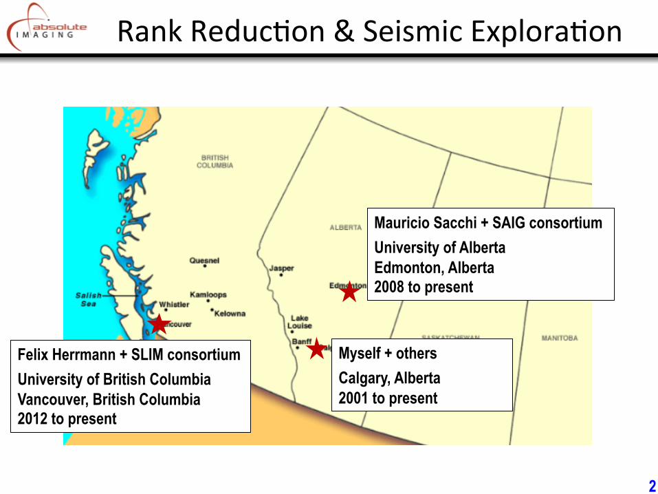
Rank  Reduc*on  &  Seismic  Explora*on  

Myself + others Calgary, Alberta 2001 to present

Mauricio Sacchi + SAIG consortium University of Alberta Edmonton, Alberta 2008 to present

Felix Herrmann + SLIM consortium University of British Columbia Vancouver, British Columbia 2012 to present

2

Topics  

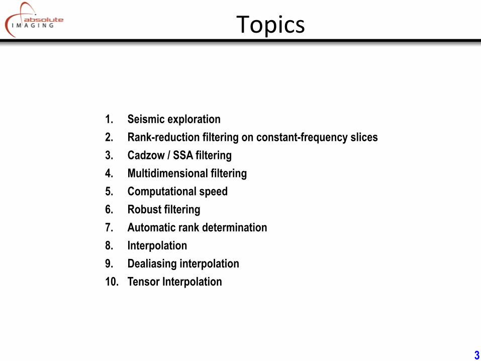
1.  Seismic exploration 2.  Rank-reduction filtering on constant-frequency slices 3.  Cadzow / SSA filtering 4.  Multidimensional filtering 5.  Computational speed 6.  Robust filtering 7.  Automatic rank determination 8.  Interpolation 9.  Dealiasing interpolation 10.  Tensor Interpolation

3

1. Seismic Exploration

4

Seismic  Explora*on  

Seismic exploration uses generated sound waves traveling within the earth to locate and develop petroleum and other

mineral resources.

$15 billion / year industry.

5

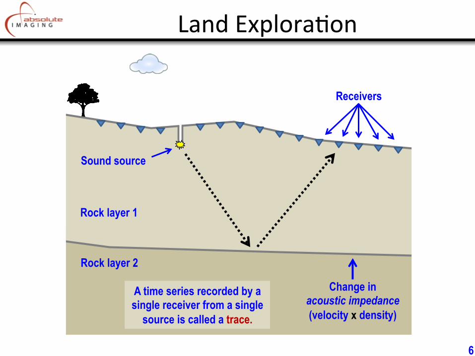
Land  Explora*on  

Rock layer 1

Rock layer 2

Sound source

Receivers

Change in acoustic impedance (velocity x density)

A time series recorded by a single receiver from a single

source is called a trace.

6

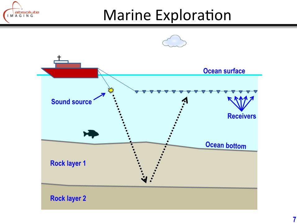
Marine  Explora*on  

Sound source

Receivers

Rock layer 1

Rock layer 2

Ocean surface

Ocean bottom

7

Survey  Sizes  

Number of recorded traces in a single seismic survey… 10 million to 100 billion. Trillion trace surveys being considered. Single survey covers an area between 5 sq km to 10,000 sq km.

8

Four  Spa*al  Dimensions  

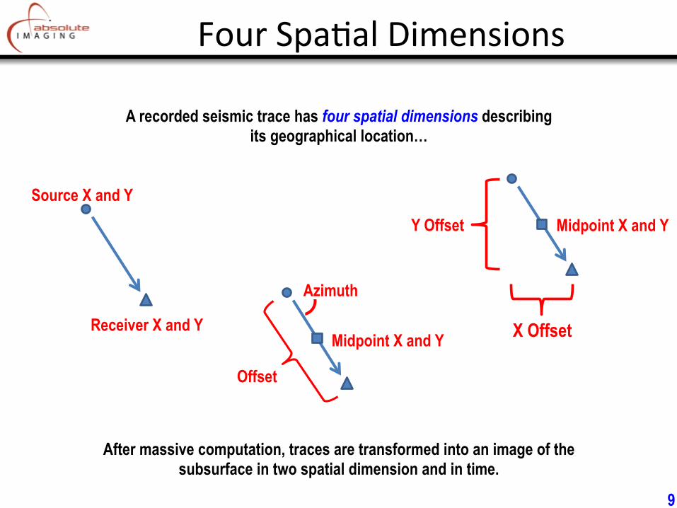
A recorded seismic trace has four spatial dimensions describing its geographical location…

Source X and Y

Receiver X and Y Midpoint X and Y

Offset

Azimuth

X Offset

Midpoint X and Y Y Offset

After massive computation, traces are transformed into an image of the subsurface in two spatial dimension and in time.

9

10

(client seismic slides removed)

2. Rank-Reduction Filtering On Constant-Frequency Slices

11

Rank-­‐Reduc*on  Filtering  

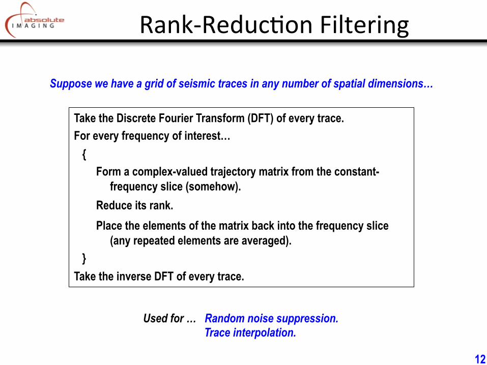
Suppose we have a grid of seismic traces in any number of spatial dimensions…

Take the Discrete Fourier Transform (DFT) of every trace. For every frequency of interest… { Form a complex-valued trajectory matrix from the constant- frequency slice (somehow). Reduce its rank. Place the elements of the matrix back into the frequency slice (any repeated elements are averaged). } Take the inverse DFT of every trace.

Used for … Random noise suppression. Trace interpolation.

12

3

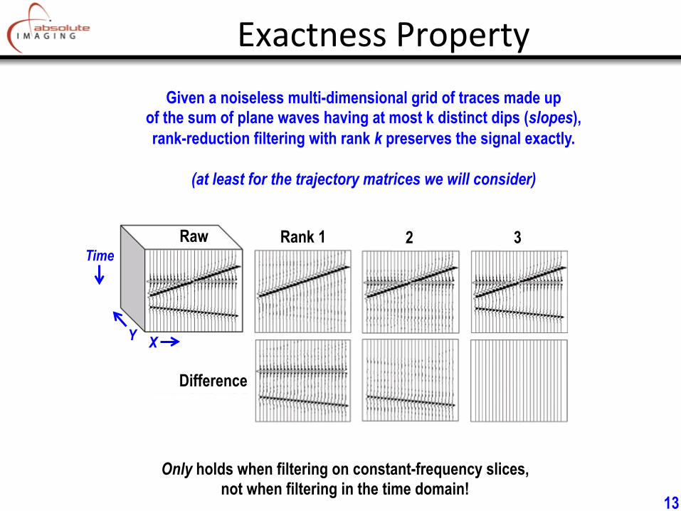
Exactness  Property  Given a noiseless multi-dimensional grid of traces made up

of the sum of plane waves having at most k distinct dips (slopes), rank-reduction filtering with rank k preserves the signal exactly.

(at least for the trajectory matrices we will consider)

Only holds when filtering on constant-frequency slices, not when filtering in the time domain!

3 2 Rank 1 Raw  Raw

Difference

Time

X Y

13

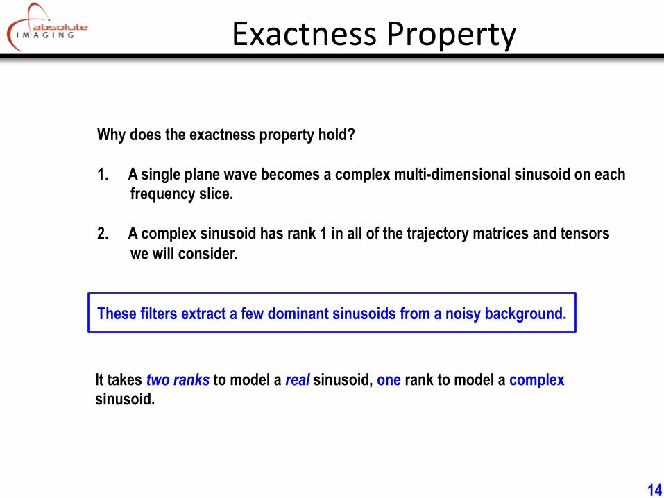
Exactness  Property  

Why does the exactness property hold? 1.  A single plane wave becomes a complex multi-dimensional sinusoid on each

frequency slice.

2.  A complex sinusoid has rank 1 in all of the trajectory matrices and tensors we will consider.

These filters extract a few dominant sinusoids from a noisy background.

It takes two ranks to model a real sinusoid, one rank to model a complex sinusoid.

14

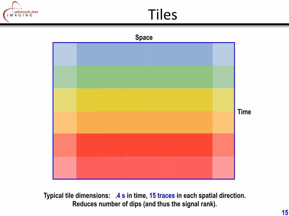
Tiles  Space

Time

Typical tile dimensions: .4 s in time, 15 traces in each spatial direction. Reduces number of dips (and thus the signal rank).

15

3. Cadzow / SSA Filtering

16

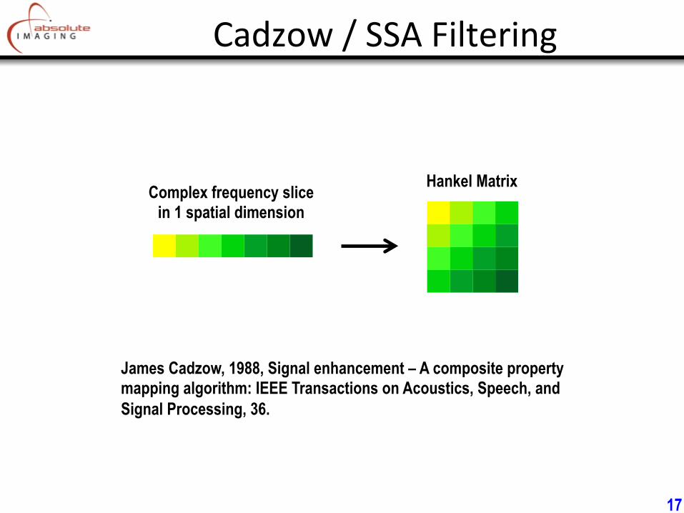
Complex frequency slice in 1 spatial dimension

Hankel Matrix

Cadzow  /  SSA  Filtering  

James Cadzow, 1988, Signal enhancement – A composite property mapping algorithm: IEEE Transactions on Acoustics, Speech, and Signal Processing, 36.

17

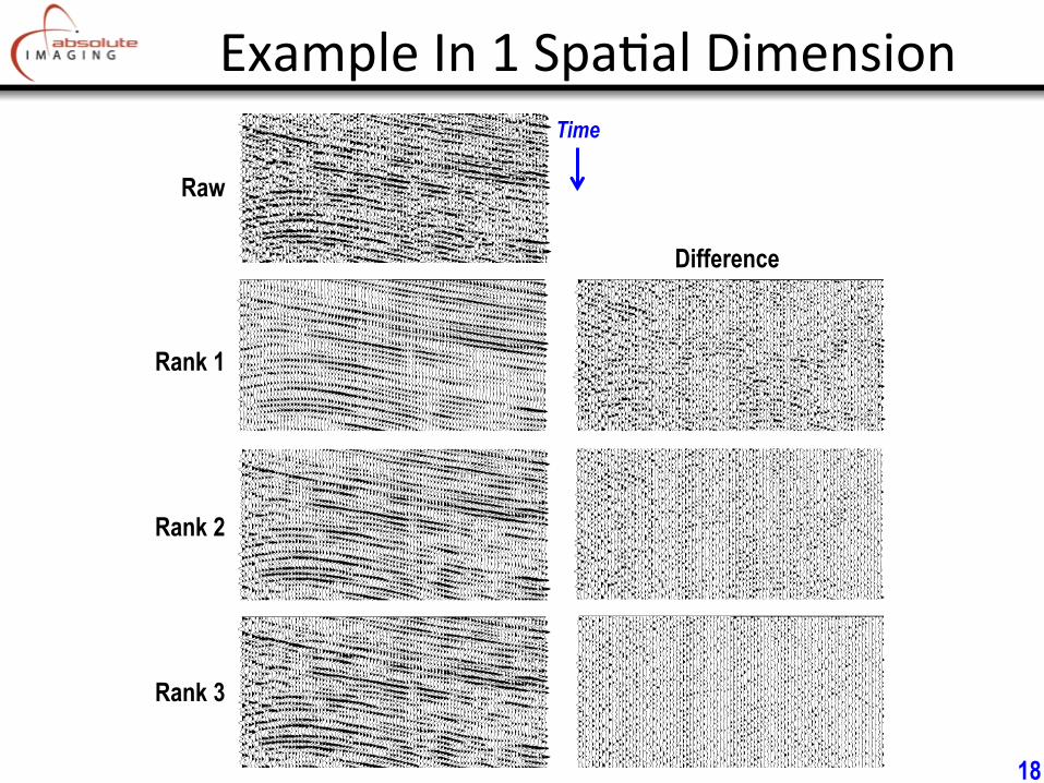
Example  In  1  Spa*al  Dimension  

Raw

Rank 1

Rank 2

Rank 3

Difference

Time

18

Cadzow  Itera*on  

19

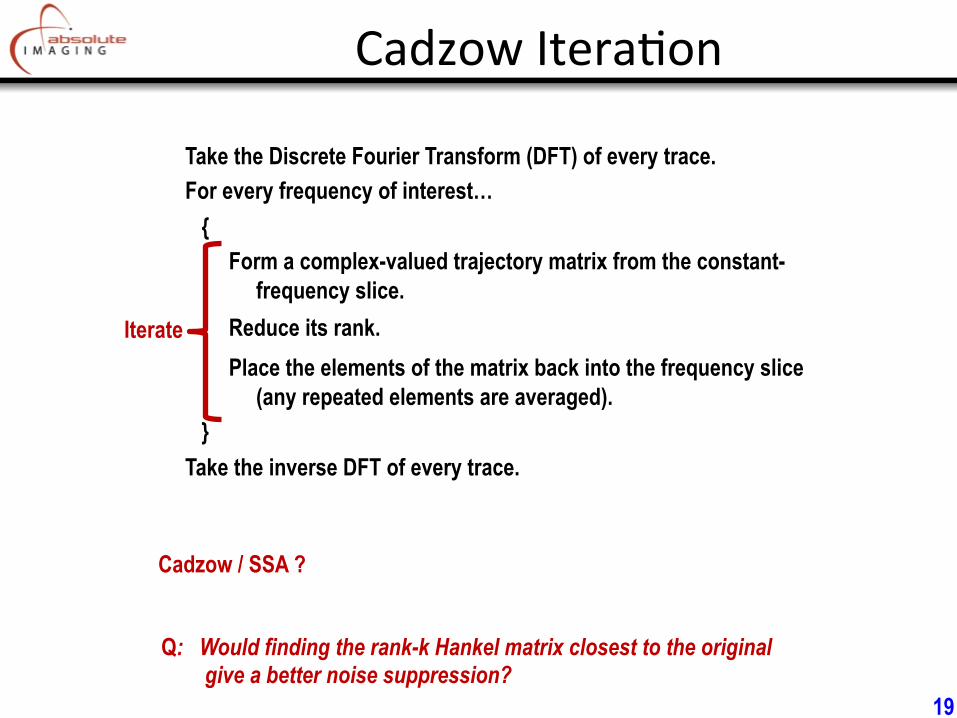
Take the Discrete Fourier Transform (DFT) of every trace. For every frequency of interest… { Form a complex-valued trajectory matrix from the constant- frequency slice. Reduce its rank. Place the elements of the matrix back into the frequency slice (any repeated elements are averaged). } Take the inverse DFT of every trace.

Iterate

Q: Would finding the rank-k Hankel matrix closest to the original give a better noise suppression?

Cadzow / SSA ?

4. Multidimensional Filtering

20

Mul*dimensional  Filtering  

Raw seismic traces have four spatial dimensions. Filtering in many spatial dimensions at once greatly increases the power of the filter. We can remove far more noise while preserving signal. How do we extend rank-reduction filtering to many dimensions?

21

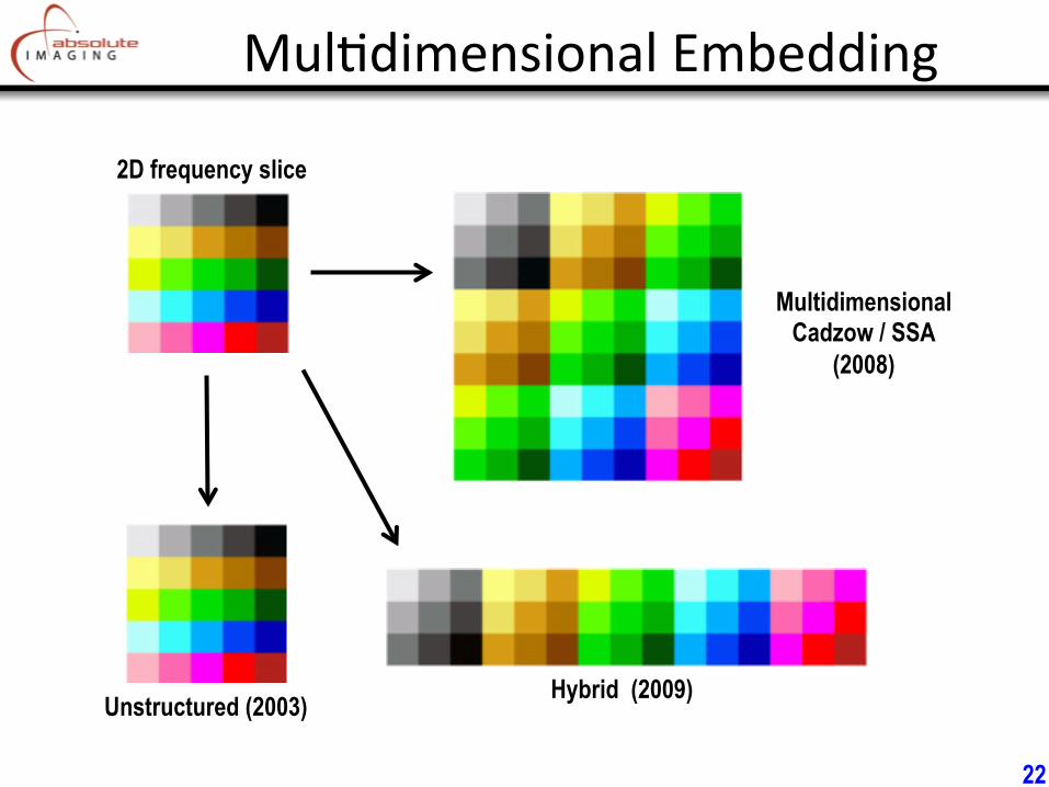
Mul*dimensional  Embedding  

2D frequency slice

Multidimensional Cadzow / SSA

(2008)

Hybrid (2009) Unstructured (2003)

22

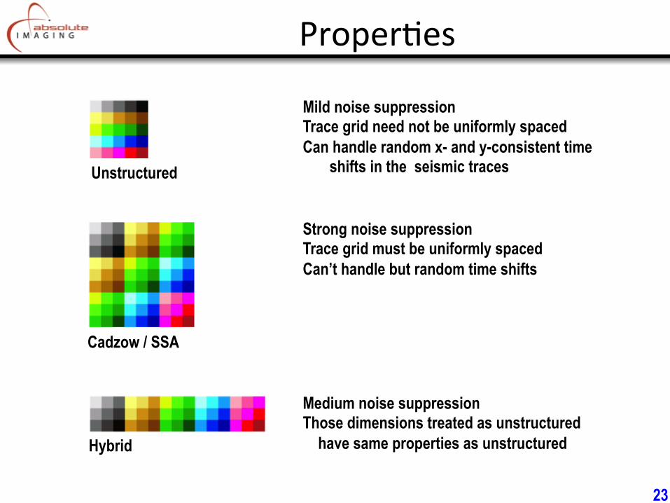
Proper*es  

Unstructured

Cadzow / SSA

Hybrid

Mild noise suppression Trace grid need not be uniformly spaced Can handle random x- and y-consistent time shifts in the seismic traces

Strong noise suppression Trace grid must be uniformly spaced Can’t handle but random time shifts

Medium noise suppression Those dimensions treated as unstructured have same properties as unstructured

23

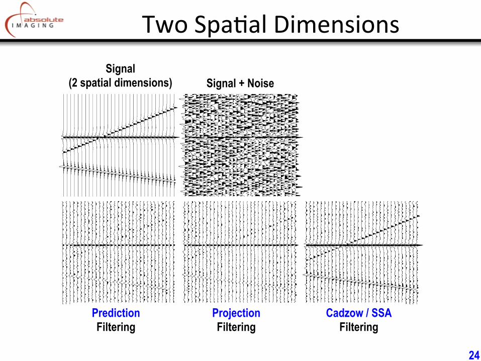
Two  Spa*al  Dimensions  Signal

(2 spatial dimensions) Signal + Noise

Prediction Filtering

Projection Filtering

Cadzow / SSA Filtering

24

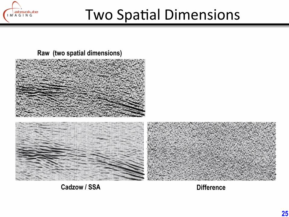
Two  Spa*al  Dimensions  

Raw (two spatial dimensions)

Cadzow / SSA Difference

25

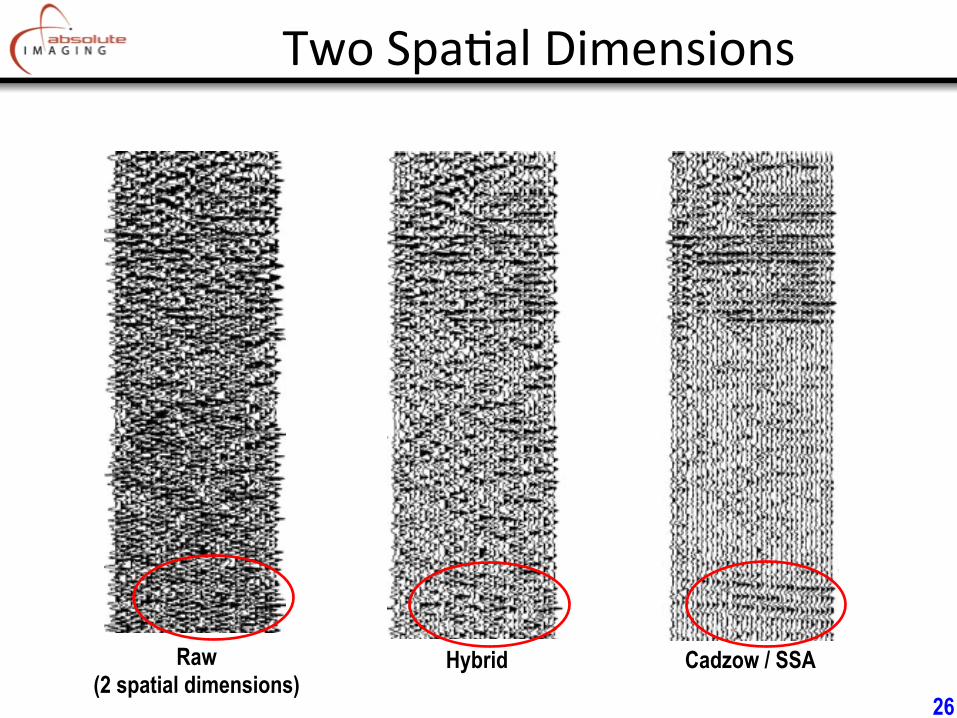
Two  Spa*al  Dimensions  

Raw (2 spatial dimensions)

Hybrid Cadzow / SSA

26

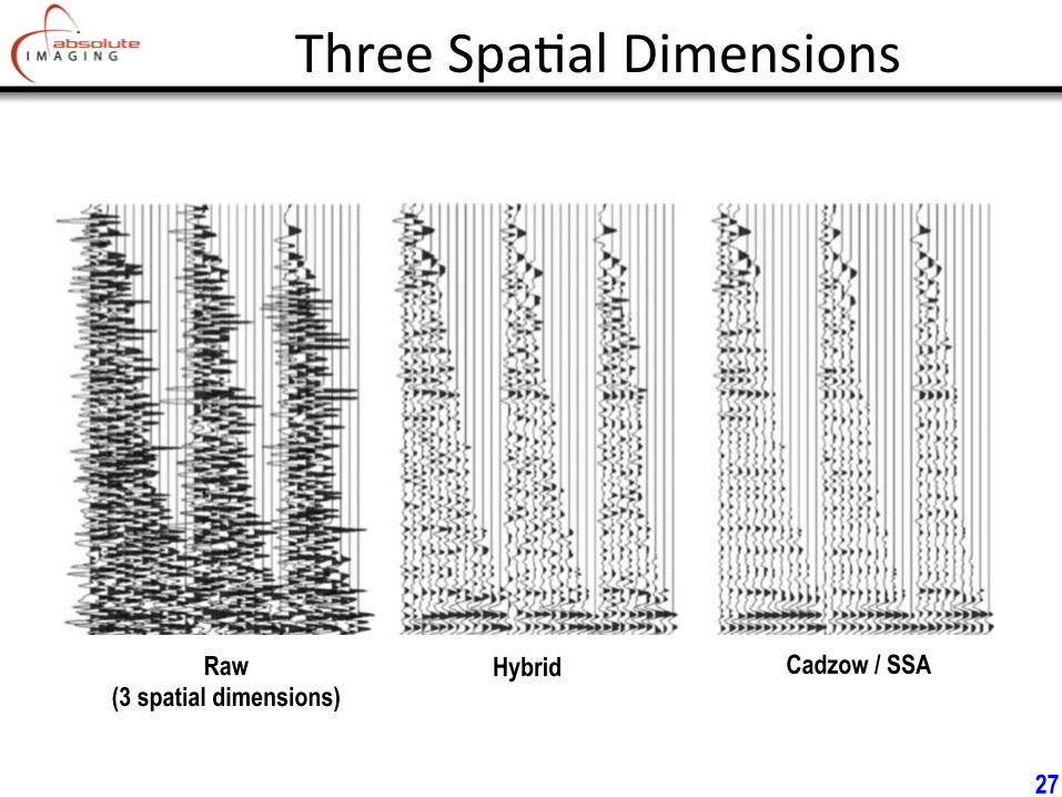
Three  Spa*al  Dimensions  

Raw (3 spatial dimensions)

Hybrid Cadzow / SSA

27

5. Computational Speed

28

Approxima*ng  The  SVD  

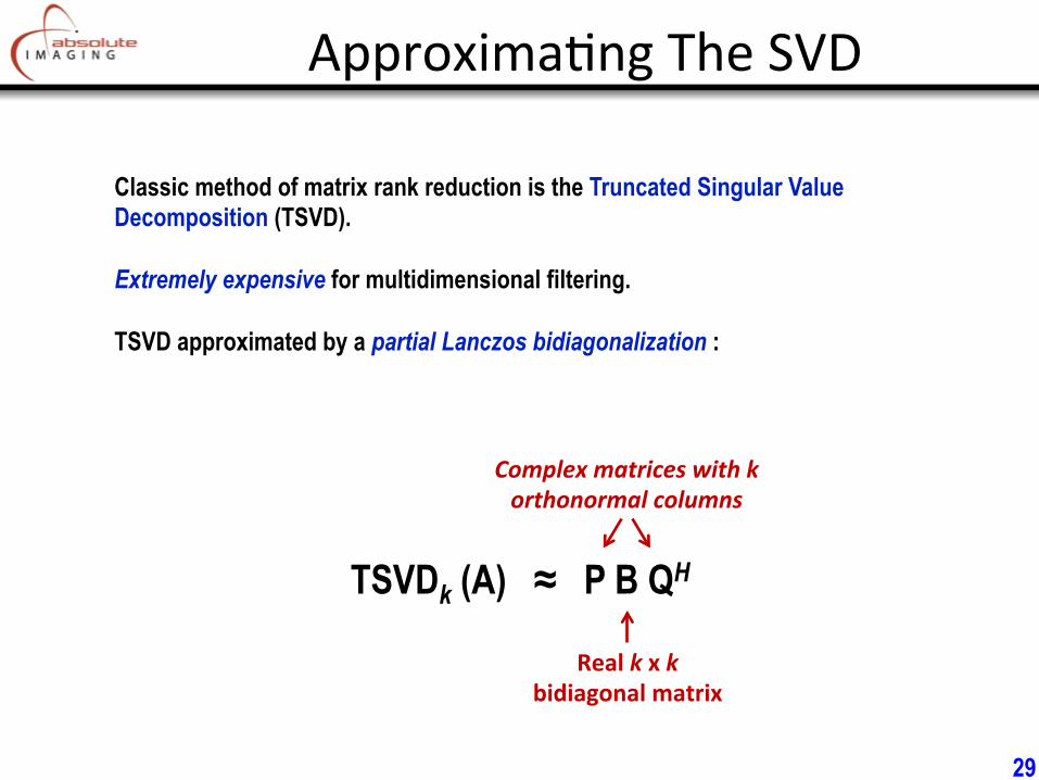
Classic method of matrix rank reduction is the Truncated Singular Value Decomposition (TSVD). Extremely expensive for multidimensional filtering. TSVD approximated by a partial Lanczos bidiagonalization :

Complex  matrices  with  k  orthonormal  columns  

Real  k  x  k  bidiagonal  matrix  

TSVDk (A) ≈ P B QH

29

Improving  Lanczos  Bidiagonaliza*on  

Partial Lanczos Bidiagonalization captures the largest singular values, but also some small (spurious) singular values. Can remove spurious singular values by… 1.  Calculate the rank k+r partial bidiagonalization, where r is some small

integer.

2.  Perform TSVD on the inner bidiagonal matrix B to reduce it to rank k.

Can prove you get a better approximation to the rank-k TSVD as r increases (in exact arithmetic).

30

Fast  Matrix  Mul*plica*on  

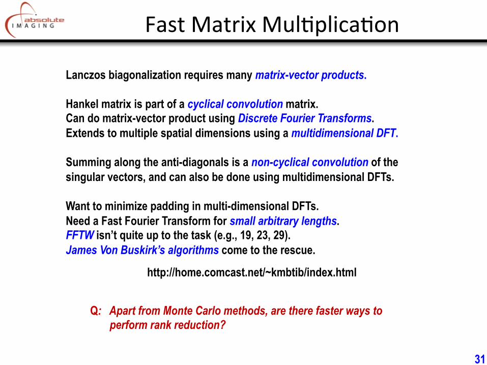
Lanczos biagonalization requires many matrix-vector products. Hankel matrix is part of a cyclical convolution matrix. Can do matrix-vector product using Discrete Fourier Transforms. Extends to multiple spatial dimensions using a multidimensional DFT. Summing along the anti-diagonals is a non-cyclical convolution of the singular vectors, and can also be done using multidimensional DFTs. Want to minimize padding in multi-dimensional DFTs. Need a Fast Fourier Transform for small arbitrary lengths. FFTW isn’t quite up to the task (e.g., 19, 23, 29). James Von Buskirk’s algorithms come to the rescue.

http://home.comcast.net/~kmbtib/index.html

Q: Apart from Monte Carlo methods, are there faster ways to perform rank reduction?

31

6. Robust Filtering

32

Erra*c  Noise  

Truncated SVD is a least-squares fit, well suited for Gaussian noise. In seismic data, noise is often erratic due to:

Air blast, powerline and other cultural noises, recording and parity errors, uncorrected polarity reversals, isolated noise bursts (often due to deconvolved spikes, zeroes, and clips), misfired shots, scattered shot noise, poor surface conditions, disabled or poorly coupled geophones, wind, rain, simultaneous shooting…

Need a statistically robust version!

33

Itera*ve  Winsoriza*on  

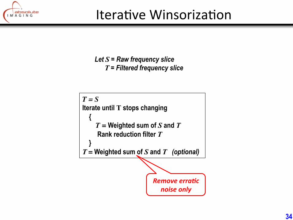
Let S = Raw frequency slice T = Filtered frequency slice

T = SIterate until T stops changing { T = Weighted sum of S and T Rank reduction filter T } T = Weighted sum of S and T (optional)

Remove  erra6c  noise  only  

34

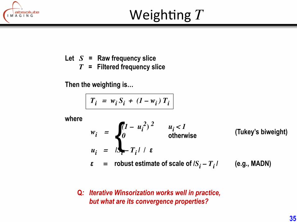
Weigh*ng  T

Let S = Raw frequency slice T = Filtered frequency slice Then the weighting is…

35

where

wi = (Tukey’s biweight)

ui = |Si – Ti | / ε

ε = robust estimate of scale of |Si – Ti | (e.g., MADN)

Q: Iterative Winsorization works well in practice, but what are its convergence properties?

{ Ti = wi Si + (1 – wi ) Ti  

 

(1 – ui2) 2 ui < 1

0 otherwise

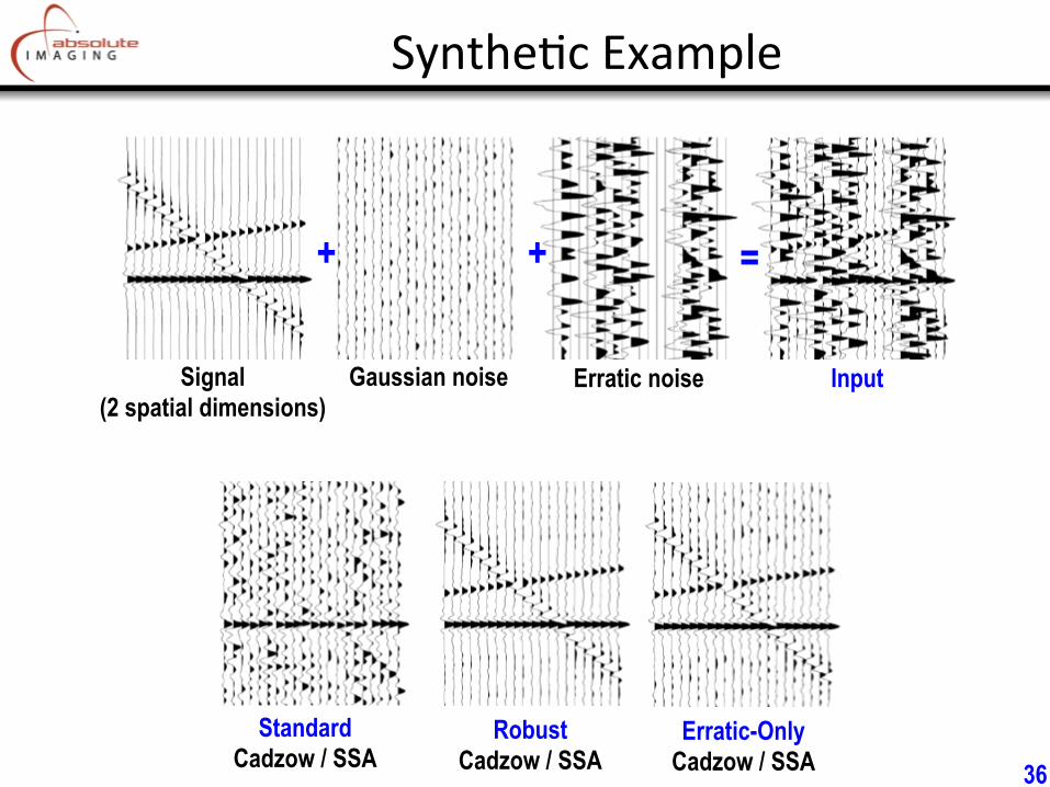
Synthe*c  Example  

Signal (2 spatial dimensions)

Gaussian noise Erratic noise Input

Standard Cadzow / SSA

Robust Cadzow / SSA

Erratic-Only Cadzow / SSA

+ + =

36

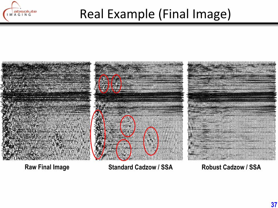
Real  Example  (Final  Image)  

Raw Final Image Robust Cadzow / SSA Standard Cadzow / SSA

37

7. Automatic Rank Determination

38

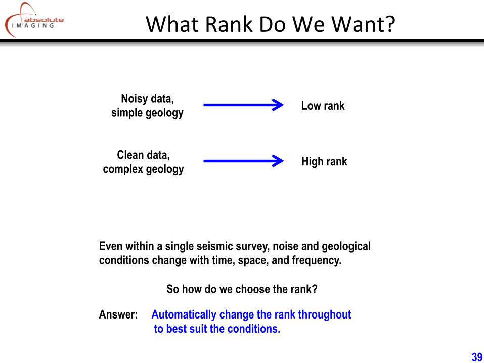
What  Rank  Do  We  Want?  

Clean data, complex geology

Noisy data, simple geology Low rank

High rank

Even within a single seismic survey, noise and geological conditions change with time, space, and frequency.

So how do we choose the rank?

39

Answer: Automatically change the rank throughout to best suit the conditions.

Automa*c  Rank  Determina*on  

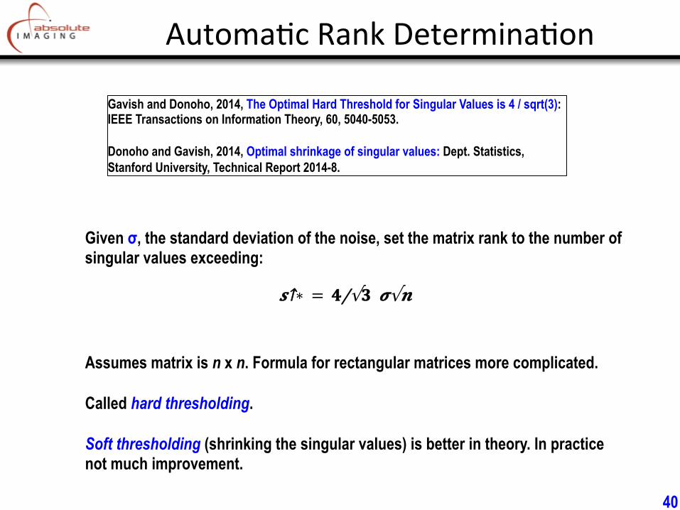
Gavish and Donoho, 2014, The Optimal Hard Threshold for Singular Values is 4 / sqrt(3): IEEE Transactions on Information Theory, 60, 5040-5053. Donoho and Gavish, 2014, Optimal shrinkage of singular values: Dept. Statistics, Stanford University, Technical Report 2014-8.

Given σ, the standard deviation of the noise, set the matrix rank to the number of singular values exceeding:

𝒔↑∗   =     𝟒/√𝟑  𝝈√𝒏   

Assumes matrix is n x n. Formula for rectangular matrices more complicated. Called hard thresholding. Soft thresholding (shrinking the singular values) is better in theory. In practice not much improvement.

40

Three  Problems  

Two problems to overcome… 1. Estimating noise level σ when full SVD is unavailable.

2. Making the filter less harsh for extreme noise.

41

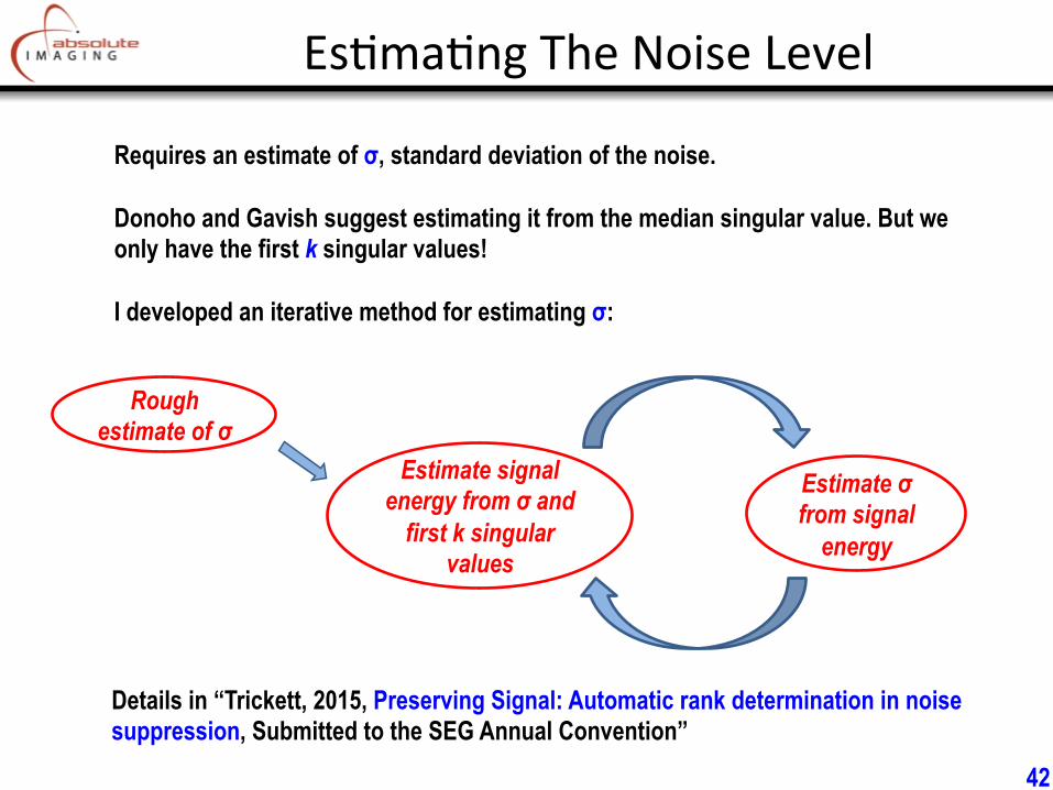
Es*ma*ng  The  Noise  Level  

Requires an estimate of σ, standard deviation of the noise. Donoho and Gavish suggest estimating it from the median singular value. But we only have the first k singular values! I developed an iterative method for estimating σ:

Estimate σ from signal

energy

Estimate signal energy from σ and

first k singular values

Details in “Trickett, 2015, Preserving Signal: Automatic rank determination in noise suppression, Submitted to the SEG Annual Convention”

Rough estimate of σ

42

Extreme  Noise  

In extreme noise, automatic rank determination can recommend not keeping any singular values (zeroing the frequency slice). Optimum in theory. Unacceptable in practice. Countless ways to fix this. Suggest limiting threshold to something less than the first singular value s1:

𝒔↑∗   =𝐦𝐢𝐧    ( 𝒔↑∗ ,  .𝟕𝟓   𝒔↓𝟏 )  

43

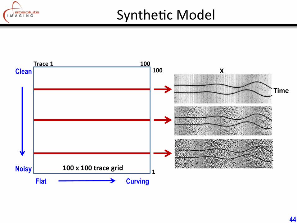
Synthe*c  Model  

Flat Curving

Trace  1   100  

1  

100  

Time  

X    Clean

Noisy

44

100  x  100  trace  grid  

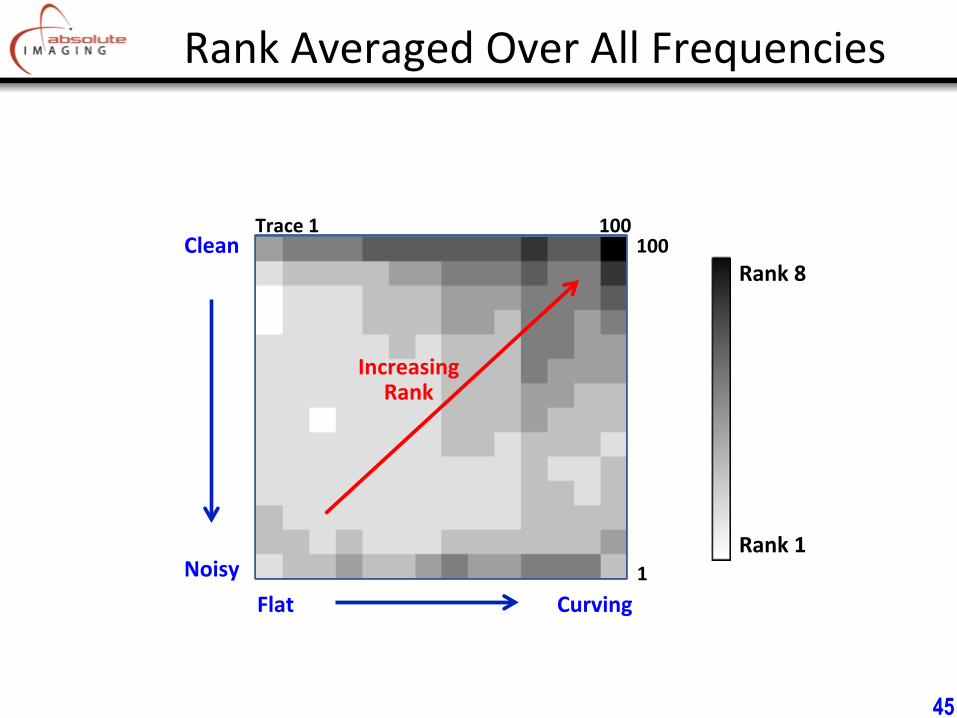
Rank  Averaged  Over  All  Frequencies  

Clean  

Noisy  Flat   Curving  

Trace  1   100  100  

1  

Rank  8  

Rank  1  

Increasing  Rank  

45

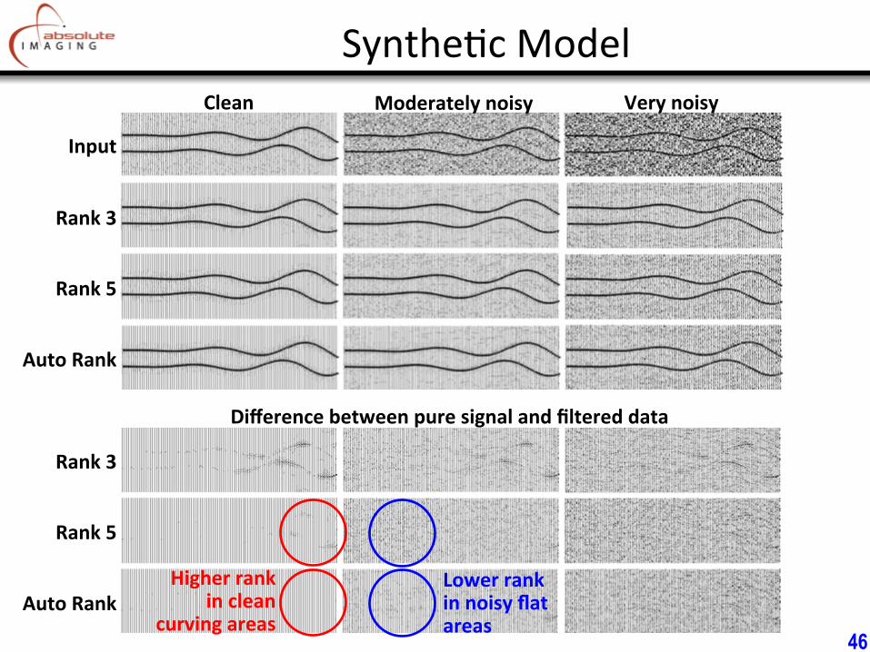
Synthe*c  Model  Clean   Moderately  noisy   Very  noisy  

Difference  between  pure  signal  and  filtered  data  

Input  

Rank  3  

Rank  5  

Auto  Rank  

Rank  3  

Rank  5  

Auto  Rank  

Higher  rank  in  clean  

curving  areas  

Lower  rank    in  noisy  flat  areas  

46

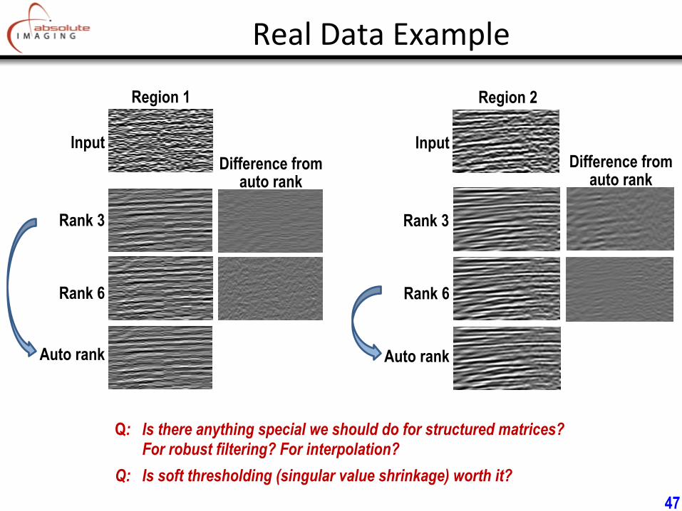
Real  Data  Example  

Region 2 Region 1

Input

Rank 3

Rank 6

Auto rank

Input

Rank 3

Rank 6

Auto rank

Difference from auto rank

Difference from auto rank

47

Q: Is there anything special we should do for structured matrices? For robust filtering? For interpolation? Q: Is soft thresholding (singular value shrinkage) worth it?

8. Interpolation

48

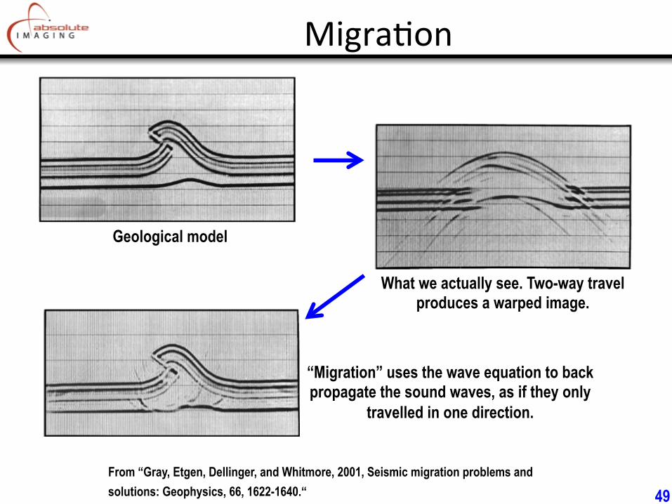
Migra*on  

What we actually see. Two-way travel produces a warped image.

Geological model

“Migration” uses the wave equation to back propagate the sound waves, as if they only

travelled in one direction.

From “Gray, Etgen, Dellinger, and Whitmore, 2001, Seismic migration problems and solutions: Geophysics, 66, 1622-1640.“ 49

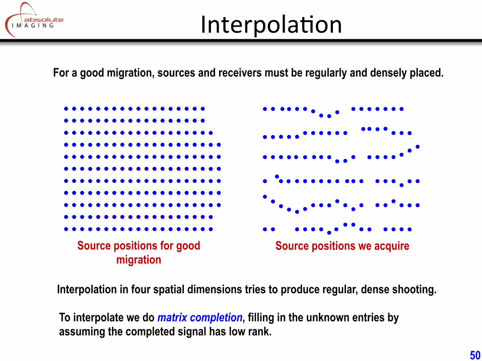
Interpola*on  

For a good migration, sources and receivers must be regularly and densely placed.

Interpolation in four spatial dimensions tries to produce regular, dense shooting.

Source positions we acquire Source positions for good migration

To interpolate we do matrix completion, filling in the unknown entries by assuming the completed signal has low rank.

50

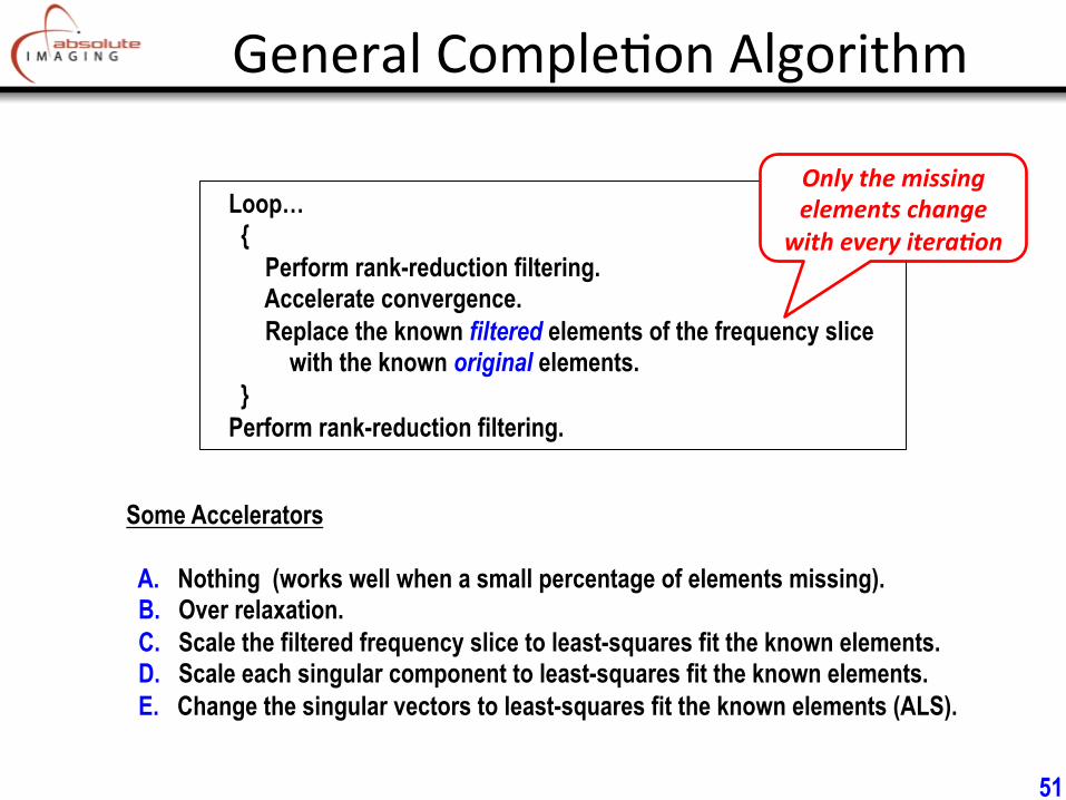
General  Comple*on  Algorithm  

Loop… { Perform rank-reduction filtering. Accelerate convergence. Replace the known filtered elements of the frequency slice with the known original elements. } Perform rank-reduction filtering.

Some Accelerators A. Nothing (works well when a small percentage of elements missing). B. Over relaxation. C. Scale the filtered frequency slice to least-squares fit the known elements. D. Scale each singular component to least-squares fit the known elements. E. Change the singular vectors to least-squares fit the known elements (ALS).

Only  the  missing  elements  change  

with  every  itera6on  

51

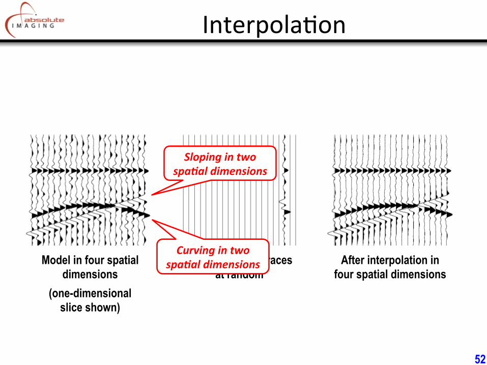
Interpola*on  

Model in four spatial dimensions

(one-dimensional slice shown)

Remove 90% of traces at random

After interpolation in four spatial dimensions

Curving  in  two  spa6al  dimensions  

Sloping  in  two  spa6al  dimensions  

52

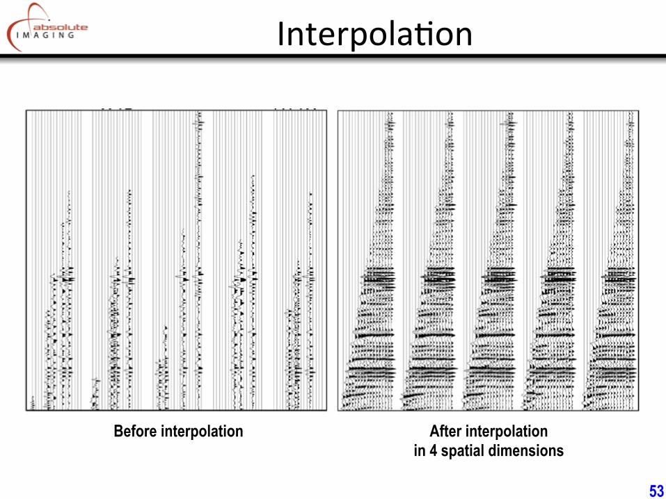
Interpola*on  

Before interpolation After interpolation in 4 spatial dimensions

53

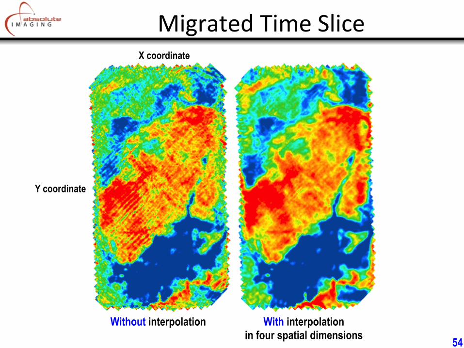
Migrated  Time  Slice  

Without interpolation With interpolation in four spatial dimensions

Y coordinate

X coordinate

54

9. Dealiasing Interpolation

55

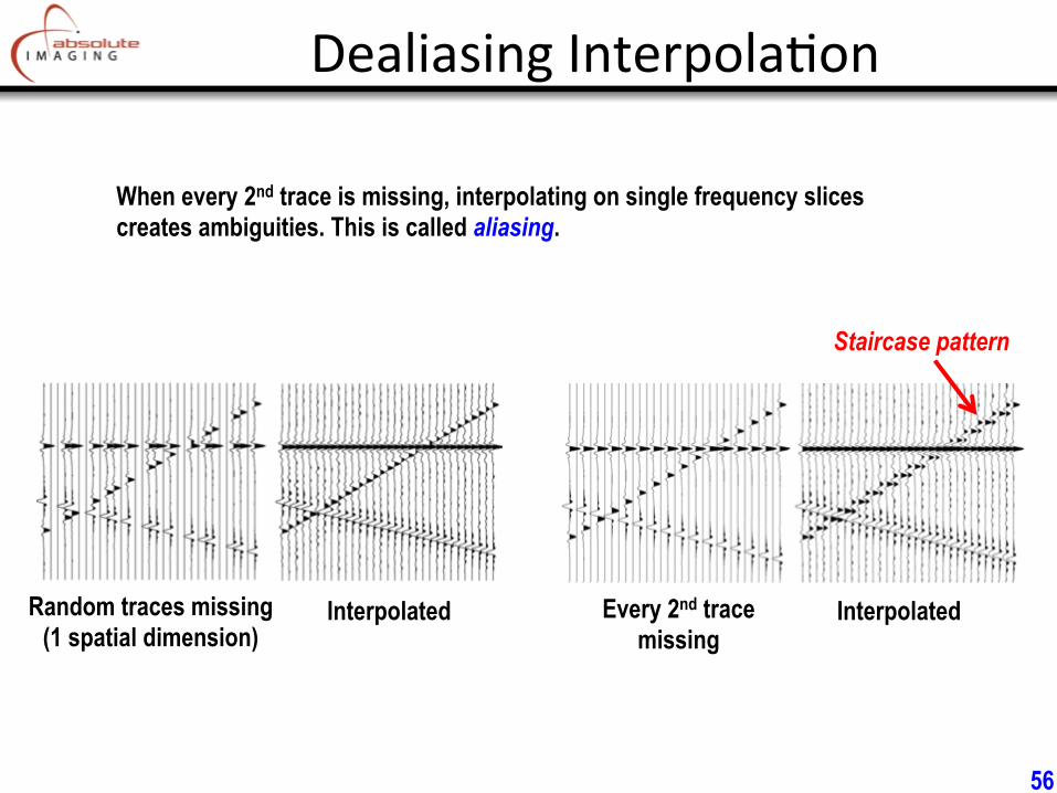
Dealiasing  Interpola*on  

When every 2nd trace is missing, interpolating on single frequency slices creates ambiguities. This is called aliasing.

Random traces missing (1 spatial dimension)

Interpolated Every 2nd trace missing

Interpolated

Staircase pattern

56

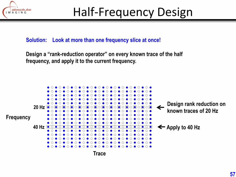
Solution: Look at more than one frequency slice at once!

Design a “rank-reduction operator” on every known trace of the half frequency, and apply it to the current frequency.

Trace

Frequency

Design rank reduction on known traces of 20 Hz

Apply to 40 Hz

20 Hz

40 Hz

Half-­‐Frequency  Design  

57

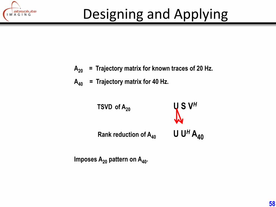
A20 = Trajectory matrix for known traces of 20 Hz.

A40 = Trajectory matrix for 40 Hz.

TSVD of A20 U S VH

Rank reduction of A40 U UH A40

Imposes A20 pattern on A40.

Designing  and  Applying  

58

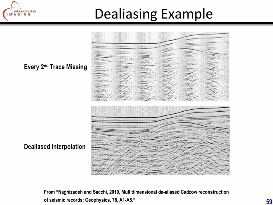
Dealiasing  Example  

Every 2nd Trace Missing

Dealiased Interpolation

From “Naghizadeh and Sacchi, 2010, Multidimensional de-aliased Cadzow reconstruction of seismic records: Geophysics, 78, A1-A5.“ 59

10. Tensor Interpolation

60

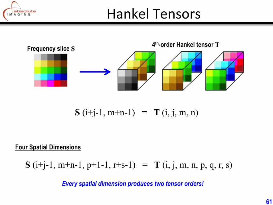
Hankel  Tensors  

Frequency slice S 4th-order Hankel tensor T

S (i+j-1, m+n-1) = T (i, j, m, n)

S (i+j-1, m+n-1, p+1-1, r+s-1) = T (i, j, m, n, p, q, r, s)

Four Spatial Dimensions

Every spatial dimension produces two tensor orders!

61

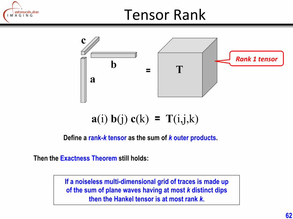
Tensor  Rank  

a(i) b(j) c(k) = T(i,j,k)

Rank  1  tensor  

Define a rank-k tensor as the sum of k outer products.

If a noiseless multi-dimensional grid of traces is made up of the sum of plane waves having at most k distinct dips

then the Hankel tensor is at most rank k.

Then the Exactness Theorem still holds:

62

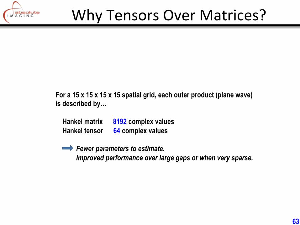
Why  Tensors  Over  Matrices?  

For a 15 x 15 x 15 x 15 spatial grid, each outer product (plane wave) is described by… Hankel matrix 8192 complex values Hankel tensor 64 complex values Fewer parameters to estimate. Improved performance over large gaps or when very sparse.

63

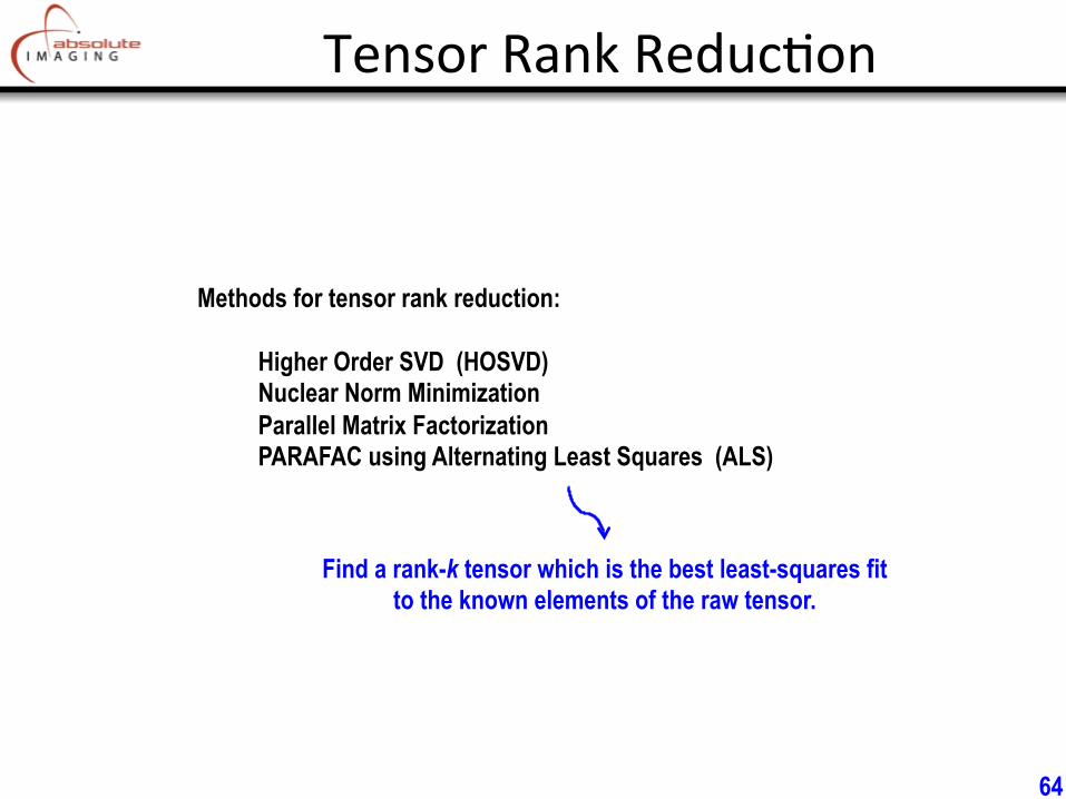
Tensor  Rank  Reduc*on  

Methods for tensor rank reduction: Higher Order SVD (HOSVD) Nuclear Norm Minimization Parallel Matrix Factorization PARAFAC using Alternating Least Squares (ALS)

Find a rank-k tensor which is the best least-squares fit to the known elements of the raw tensor.

64

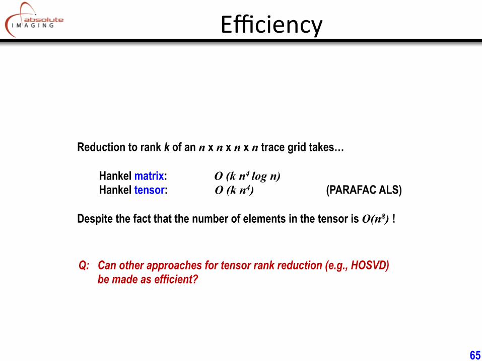
Efficiency  

Reduction to rank k of an n x n x n x n trace grid takes… Hankel matrix: O (k n4 log n) Hankel tensor: O (k n4) (PARAFAC ALS) Despite the fact that the number of elements in the tensor is O(n8) !

65

Q: Can other approaches for tensor rank reduction (e.g., HOSVD) be made as efficient?

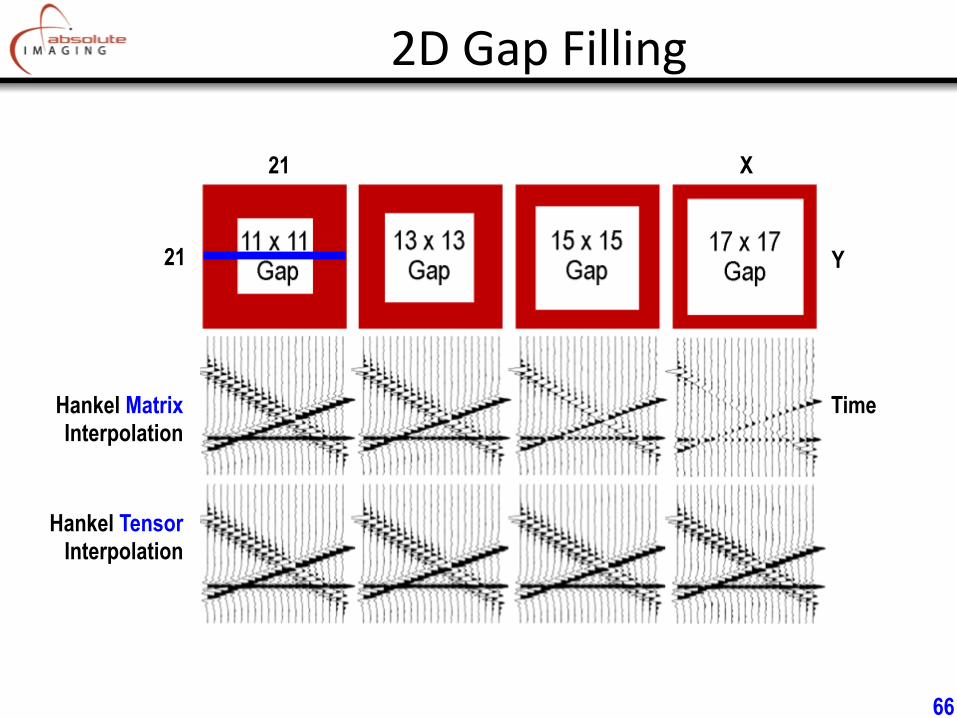
2D  Gap  Filling  

X

Y

Time Hankel Matrix Interpolation

Hankel Tensor Interpolation

21

21

66

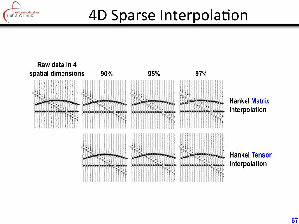
4D  Sparse  Interpola*on  

Hankel Matrix Interpolation

Hankel Tensor Interpolation

Raw data in 4 spatial dimensions 90% 95% 97%

67

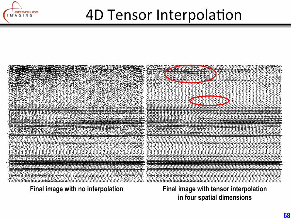
4D  Tensor  Interpola*on  

Final image with no interpolation Final image with tensor interpolation in four spatial dimensions

68

Thanks to…

Canadian Society of Exploration Geophysicists

Society of Exploration Geophysicists

Cadzow  and  SSA  

Purpose of inner loop is to find the rank-k Hankel matrix closest to the original data Hankel matrix. Inner loop proven to converge, but not necessarily to the closest rank-k Hankel matrix. Multiplied cost without improving result. Sacchi (2009) pointed out that without the inner loop, “Cadzow filtering” was equivalent Singular Spectrum Analysis (SSA). Now we don’t know what to call the method. Cadzow / SSA?

Q: Would finding the rank-k Hankel matrix closest to the original give a better noise suppression?

70