university of copenhagen Ørsted · resume17´ abbreviations, notation, and units 19 i...

University of Copenhagen Ørsted•DTUFaculty of Health Sciences Center forDept. of Ultrasound Fast Ultrasound ImagingHerlev Hospital

Ph.D. Thesis

New Digital Techniques in MedicalUltrasound Scanning

Morten Høgholm Pedersen

July 4, 2003

Advisor:Prof. Dr. Med. Bjørn Quistorff

Project advisors:Dr. Med. Torben Larsen

Prof. Dr. Techn. Jørgen Arendt Jensen

to Karin

my Love

5

Contents Overview

Preface 11

Acknowledgements 13

Summary 15

Resume 17

Abbreviations, Notation, and Units 19

I Three-Dimensional Ultrasound Imaging 21

1 Ultrasound and 3D Imaging 23

2 Clinical Use of 3DUS 37

II Clinical Trial: 3DUS of Cervical Cancer 45

3 Introduction 47

4 Material and Methods 55

5 Results 71

6 Discussion 95

III Pre-clinical trial: Coded Excitation 103

7 Introduction 107

8 Material and Methods 117

9 Results 129

10 Discussion 133

IV Conclusion 135

11 Overall Discussion and Perspectives 137

V Appendices and Bibliography 141

A FIGO Stages 143

B The Cohen Kappa Value 145

C Software Documentation 147

D Publications 153

Bibliography 181

6 CONTENTS OVERVIEW

7

Contents

Preface 11

Acknowledgements 13

Summary 15

Resume 17

Abbreviations, Notation, and Units 19

I Three-Dimensional Ultrasound Imaging 21

1 Ultrasound and 3D Imaging 231.1 Ultrasound . . . . . . . . . . . . . . . . . . . . . . . . . . . . . . . . . 231.2 Ultrasound Scanning . . . . . . . . . . . . . . . . . . . . . . . . . . . 24

1.2.1 Attenuation and Time Gain Compensation . . . . . . . . . . . . 251.2.2 Resolution . . . . . . . . . . . . . . . . . . . . . . . . . . . . 271.2.3 Dynamic Images and Framerate . . . . . . . . . . . . . . . . . 27

1.3 3D Imaging . . . . . . . . . . . . . . . . . . . . . . . . . . . . . . . . 281.4 3D Visualization . . . . . . . . . . . . . . . . . . . . . . . . . . . . . 29

1.4.1 Depth Cues . . . . . . . . . . . . . . . . . . . . . . . . . . . . 291.4.2 Surface Rendering and Segmentation . . . . . . . . . . . . . . 291.4.3 Volume Rendering . . . . . . . . . . . . . . . . . . . . . . . . 301.4.4 Slicing and Intersecting Planes . . . . . . . . . . . . . . . . . . 31

1.5 3D Ultrasound Scanning and Visualization . . . . . . . . . . . . . . . . 311.6 3DUS Visualization and Software . . . . . . . . . . . . . . . . . . . . 34

2 Clinical Use of 3DUS 372.1 3DUS and Specialities . . . . . . . . . . . . . . . . . . . . . . . . . . 372.2 3DUS in Obstetrics . . . . . . . . . . . . . . . . . . . . . . . . . . . . 402.3 3DUS in Gynecology . . . . . . . . . . . . . . . . . . . . . . . . . . . 42

II Clinical Trial: 3DUS of Cervical Cancer 45

3 Introduction 473.1 Pathogenesis, Pathology, and Epidemiology . . . . . . . . . . . . . . . 483.2 Disease . . . . . . . . . . . . . . . . . . . . . . . . . . . . . . . . . . 483.3 Staging . . . . . . . . . . . . . . . . . . . . . . . . . . . . . . . . . . 483.4 Treatment . . . . . . . . . . . . . . . . . . . . . . . . . . . . . . . . . 49

8 Contents

3.5 Prognosis . . . . . . . . . . . . . . . . . . . . . . . . . . . . . . . . . 493.6 Imaging . . . . . . . . . . . . . . . . . . . . . . . . . . . . . . . . . . 503.7 Ultrasound Scanning . . . . . . . . . . . . . . . . . . . . . . . . . . . 503.8 Aim of Study . . . . . . . . . . . . . . . . . . . . . . . . . . . . . . . 52

4 Material and Methods 554.1 Study Design . . . . . . . . . . . . . . . . . . . . . . . . . . . . . . . 55

4.1.1 Patients . . . . . . . . . . . . . . . . . . . . . . . . . . . . . . 554.1.2 Inclusion Criteria . . . . . . . . . . . . . . . . . . . . . . . . . 554.1.3 Exclusion . . . . . . . . . . . . . . . . . . . . . . . . . . . . . 574.1.4 Contraindications and Drop-outs . . . . . . . . . . . . . . . . . 574.1.5 Measurement Parameters . . . . . . . . . . . . . . . . . . . . . 574.1.6 Power Calculations . . . . . . . . . . . . . . . . . . . . . . . . 58

4.2 Conventional Ultrasound Scanning . . . . . . . . . . . . . . . . . . . . 584.2.1 Equipment . . . . . . . . . . . . . . . . . . . . . . . . . . . . 584.2.2 Procedure . . . . . . . . . . . . . . . . . . . . . . . . . . . . . 59

4.3 Three-dimensional US Scanning . . . . . . . . . . . . . . . . . . . . . 594.3.1 Equipment . . . . . . . . . . . . . . . . . . . . . . . . . . . . 594.3.2 Acquisition . . . . . . . . . . . . . . . . . . . . . . . . . . . . 604.3.3 Registration of Results . . . . . . . . . . . . . . . . . . . . . . 61

4.4 Clinical Staging . . . . . . . . . . . . . . . . . . . . . . . . . . . . . . 624.5 MRI . . . . . . . . . . . . . . . . . . . . . . . . . . . . . . . . . . . . 62

4.5.1 Equipment and Methods . . . . . . . . . . . . . . . . . . . . . 624.5.2 Registration of Results . . . . . . . . . . . . . . . . . . . . . . 63

4.6 Pathological Evaluation - Gold Standard . . . . . . . . . . . . . . . . . 634.7 Blinding . . . . . . . . . . . . . . . . . . . . . . . . . . . . . . . . . . 644.8 Trial Approval, Safety, and Patient Strain . . . . . . . . . . . . . . . . 64

4.8.1 Ultrasound Safety . . . . . . . . . . . . . . . . . . . . . . . . . 644.8.2 MRI Safety . . . . . . . . . . . . . . . . . . . . . . . . . . . . 644.8.3 Influence on Treatment . . . . . . . . . . . . . . . . . . . . . . 654.8.4 Data Integrity and Security . . . . . . . . . . . . . . . . . . . . 65

4.9 Data Analysis . . . . . . . . . . . . . . . . . . . . . . . . . . . . . . . 654.9.1 Data Format Conversion Tool . . . . . . . . . . . . . . . . . . 654.9.2 3DUS Evaluation . . . . . . . . . . . . . . . . . . . . . . . . . 664.9.3 3DUS volume Measurements . . . . . . . . . . . . . . . . . . 674.9.4 MRI Evaluation . . . . . . . . . . . . . . . . . . . . . . . . . . 674.9.5 Assembling Histological Slices . . . . . . . . . . . . . . . . . 68

5 Results 715.1 3DUS Imaging . . . . . . . . . . . . . . . . . . . . . . . . . . . . . . 725.2 Comparison between 3DUS and Clinical Staging . . . . . . . . . . . . 745.3 Comparing to Histology Results . . . . . . . . . . . . . . . . . . . . . 785.4 Imaging after Conization . . . . . . . . . . . . . . . . . . . . . . . . . 785.5 Tumor Volume . . . . . . . . . . . . . . . . . . . . . . . . . . . . . . 795.6 Tumor Location Comparison . . . . . . . . . . . . . . . . . . . . . . . 815.7 MRI Results . . . . . . . . . . . . . . . . . . . . . . . . . . . . . . . . 825.8 Comparison of Tumor Morphology . . . . . . . . . . . . . . . . . . . . 835.9 Addendum - Case Story . . . . . . . . . . . . . . . . . . . . . . . . . . 84

Contents 9

6 Discussion 956.1 Patient Participation . . . . . . . . . . . . . . . . . . . . . . . . . . . . 96

6.2 Technical Problems . . . . . . . . . . . . . . . . . . . . . . . . . . . . 96

6.3 Image Acquisition . . . . . . . . . . . . . . . . . . . . . . . . . . . . . 97

6.4 Comparison to Histology and MRI . . . . . . . . . . . . . . . . . . . . 97

6.5 3DUS Evaluation . . . . . . . . . . . . . . . . . . . . . . . . . . . . . 98

6.6 Bladder and Rectal Invasion . . . . . . . . . . . . . . . . . . . . . . . 99

6.7 Tumor Size and Limitations . . . . . . . . . . . . . . . . . . . . . . . 99

6.8 Conization . . . . . . . . . . . . . . . . . . . . . . . . . . . . . . . . . 100

6.9 Clinical use . . . . . . . . . . . . . . . . . . . . . . . . . . . . . . . . 100

6.10 Improved Trial Protocol - Suggestion . . . . . . . . . . . . . . . . . . . 100

6.11 Conclusion . . . . . . . . . . . . . . . . . . . . . . . . . . . . . . . . 101

III Pre-clinical trial: Coded Excitation 103

7 Introduction 1077.1 Aim . . . . . . . . . . . . . . . . . . . . . . . . . . . . . . . . . . . . 108

7.2 Coded Excitation . . . . . . . . . . . . . . . . . . . . . . . . . . . . . 108

7.3 Signal-to-noise Ratio . . . . . . . . . . . . . . . . . . . . . . . . . . . 109

7.4 Duration and Bandwidth . . . . . . . . . . . . . . . . . . . . . . . . . 109

7.5 Modulation . . . . . . . . . . . . . . . . . . . . . . . . . . . . . . . . 110

7.6 Pulse Compression . . . . . . . . . . . . . . . . . . . . . . . . . . . . 112

7.7 Temporal Sidelobes . . . . . . . . . . . . . . . . . . . . . . . . . . . . 114

7.8 Expected SNR Improvement . . . . . . . . . . . . . . . . . . . . . . . 115

8 Material and Methods 1178.1 Equipment . . . . . . . . . . . . . . . . . . . . . . . . . . . . . . . . . 117

8.2 Pulses and Intensities . . . . . . . . . . . . . . . . . . . . . . . . . . . 118

8.3 Acquisition . . . . . . . . . . . . . . . . . . . . . . . . . . . . . . . . 121

8.4 Data Processing . . . . . . . . . . . . . . . . . . . . . . . . . . . . . . 121

8.5 Automatic TGC Post-Correction . . . . . . . . . . . . . . . . . . . . . 122

8.6 Image Assessment . . . . . . . . . . . . . . . . . . . . . . . . . . . . 124

8.7 Estimation of Penetration Depth . . . . . . . . . . . . . . . . . . . . . 124

8.8 Image Quality Comparison . . . . . . . . . . . . . . . . . . . . . . . . 125

8.9 Statistical Analysis . . . . . . . . . . . . . . . . . . . . . . . . . . . . 126

9 Results 1299.1 Limitations and Artifacts . . . . . . . . . . . . . . . . . . . . . . . . . 129

9.2 Penetration . . . . . . . . . . . . . . . . . . . . . . . . . . . . . . . . 130

9.3 Image Quality . . . . . . . . . . . . . . . . . . . . . . . . . . . . . . . 130

10 Discussion 133

IV Conclusion 135

10 Contents

11 Overall Discussion and Perspectives 13711.1 3D Ultrasound Scanning of Cervix Cancer . . . . . . . . . . . . . . . . 13711.2 Coded Excitation . . . . . . . . . . . . . . . . . . . . . . . . . . . . . 13811.3 Perspectives . . . . . . . . . . . . . . . . . . . . . . . . . . . . . . . . 139

V Appendices and Bibliography 141

A FIGO Stages 143

B The Cohen Kappa Value 145

C Software Documentation 147C.1 Image Registration Tool . . . . . . . . . . . . . . . . . . . . . . . . . . 148C.2 3D Data Conversion . . . . . . . . . . . . . . . . . . . . . . . . . . . . 149C.3 Raw Binary Data Format . . . . . . . . . . . . . . . . . . . . . . . . . 149C.4 Signal Processing and Movie Creation . . . . . . . . . . . . . . . . . . 152

D Publications 153D.1 Review Paper: 3DUS in Obstetrics & Gynecology . . . . . . . . . . . . 153D.2 Case Report: 3DUS of Monoamniotic Twins . . . . . . . . . . . . . . . 163D.3 Paper: Chirp Coded Excitation in US . . . . . . . . . . . . . . . . . . . 167D.4 Related Publications . . . . . . . . . . . . . . . . . . . . . . . . . . . 180D.5 Presentations . . . . . . . . . . . . . . . . . . . . . . . . . . . . . . . 180

Bibliography 181

11

Preface

”New Digital Techniques in Medical Ultrasound Scanning” is derived from the fact thatmost if not all new imaging techniques in medical ultrasound scanning heavily dependon new possibilities in computers and other digital electronics.

This work was initiated from the Center of Fast Ultrasound Imaging (CFU), located atthe Technical University of Denmark (DTU) with Prof. Dr. Techn. Jørgen Arendt Jensenas head, in collaboration with the medical ultrasound manufacturer B-K Medical A/Sand the former dept. of Ultrasound at Herlev Hospital.

The purpose of the center is to develop fast imaging methods and create better flowimages. At the moment of writing, several new methods have been developed, e.g. codedexcitation, synthetic aperture imaging, different transverse flow methods. In combina-tion they will most likely be able to produce real time three-dimensional high-resolutiongray-scale and flow images. At CFU an experimental ultrasound scanner have beendeveloped from ground up making investigation of almost all kinds of imaginable ultra-sound imaging methods possible. This includes in-vivo clinical trials.

Since real-time three-dimensional imaging always have been ’the right’ way in myeyes, and since the techniques developed at CFU ultimately will end up with that, it wasnatural to start out investigating some of the current technology and its possibilities.

Three-dimensional ultrasound has been proposed and tried for almost half a centuryago [1–5]. But not until the later years it has been clinically feasible, and all availablesystems are enabled by powerful computer systems. This thesis gives a review of three-dimensional ultrasound imaging (3DUS) with a special focus on 3DUS within obstetricsand gynecology. Then a clinical trial evaluating transrectal 3DUS in cervical cancer ispresented.

One of the techniques developed at CFU and now abundantly used with other tech-niques under development is coded excitation. Simulations and laboratory test showgreat improvement in signal-to-noise ratio with this method, but would it perform in-vivo? That was the question of the second part of this thesis, were coded excitation wereevaluated on healthy volunteers.

This work was supported by grant 9700883 and 9700563 from the Danish ScienceFoundation and by B-K Medical A/S.

12 Preface

13

Acknowledgements

I would like to thank several people for invaluable help and friendliness during the lastyears when I was struggling with this work. The following acknowledgement will makeany Oscar reward speech seem minute.

First of all I would like to thank professor MD DMSc Hans Henrik Holm, the fatherof Danish ultrasound in medicine, for initially engaging me in this work and being amost inspiring advisor.

CP MD DMSc Torben Larsen for invaluable encouragement, help, and inspirationduring the project as my primary project advisor and until recently head of the Dept.of Ultrasound, Herlev Hospital - my professional and scientific home from 1999 until itwas engulfed at the end of 2002.

Professor MSc DTSc Jørgen Arendt Jensen for initiating the work involving meas the only medical doctor in the Center for Fast Ultrasound Imaging at the TechnicalUniversity of Denmark, providing one of the most interesting and innovative biomedicalresearch environments existing today.

Thanks to professor MD DMSc Bjørn Quistorff, who has served as my advisor onseveral occasions since 1993 - during medical school, during full-time research at theNMR Center, University of Copenhagen 1993-4, and finally now taking over the role asmain advisor after Hans Henrik Holm’s retirement in 2001.

A great thankyou to all clinical partners in the planning phase and during the clinicaltrial. At the dept. of gynecology a thanks to CP MD DMSc Benny Andreasson andespecially CP MD PhD Connie Palle for her invaluable help. Also thanks to the doctorsand nurses at the dept. of gynecology for including and evaluating patients.

Thanks to doctors at the dept. of Pathology for preparing and evaluating and prepar-ing tissue to create histological data. Especially DC PhD Beth Bjerregaard for herreadiness and engagement.

CP MD DMSc Carsten Thomsen at Dept. of Diagnostic Imaging, Rigshospitalet,who were so kind to make MR scanners and equipment available to me just like that,when Herlev Hospital were not able to. Also thanks to CP MD Ajay M. Chauhan forhis help and engagement in a part of the trial that never really became.

MSc PhD Markus Nowak Lonsdale, my old friend from la dolce vita at the NMRCenter, for helping me extracting and converting MR data from scanners.

A special thanks to all earlier employees at the former dept. of Ultrasound at HerlevHospital for their warm reception of me starting out in the ultrasound field. It goes forall nurses, secretaries, and doctors without exception. I would specially like to mentionmy good colleague and office mate SS MD Nis Nørgaard and not least SS MD BjørnSkjoldbye who has been very enthusiastic teaching me diagnostic and interventionalultrasound

And of course a thank to all the patients being willing to participate in the clinicaltrial, and to the volunteers participating in the study of coded excitation.

14 Acknowledgements

PhD MSc Thanassis Misaridis for preparing my way in coded excitation. MSc KimL. Gammelmark for chewing the FDA and AUIM documentation on intensity measure-ments with me and helping performing the measurements as shown on national televi-sion.

All my current and former good colleagues at CFU for contributing to an enthusiasticatmosphere Peter Munk, Malene Schlaikjer, Svetoslav I. Nikolov, Borislav G. To-mov, Louse K. Taylor, Jesper Udesen, Frederik Gran, and Paul D. Fox (all skilledresearches with lots of fine academic titles).

Associate professor MD Jørgen Hilden and assistant professor MSc Charlotte Hinds-berger for a statistical kick-start in both projects.

Professor of medicine PhD Olaf von Ramm, PhD MSc Dr. Patrick Wolf, and MDManish Assar at Center for Emerging Cardiovascular Technology, Duke University forletting me stay for some very interesting weeks at your lab.

A thanks to Bjørn Fortling and Robert H. Owen from B-K Medical for lending methe L3Di viewer. PhD FCCPM Aaron Fenster for giving me access to the LIS fileformat. Rolf Nejsum, Cephalon A/S for supplying the 3D View 2000 program and PhDArmin Schoisswohl, Kretztechnik now GE Medical for information on the Kretz fileformat.

Karina and Poul for letting me snore in their basement during the final composingof this document.

My parents for everything. My sister and graphics designer Lise Høgholm Pedersenfor designing the cover.

Finally the greatest possible thanks to my dearly beloved wife Karin to who I amgreatly indebted for standing me, my geeky way of living, and for making this, at sev-eral occasions enervating, project possible. Thankyou for being to our children what noone else can. I am looking forward to see you all :-) Thanks to Magnus and Mikkel forbearing with me when I was only interested in ’voksen-kedeligt’.

In case I have forgot anyone here I, sincerely apologize - God sees all.

Title Abbreviations

CP Chief Physisian (Overlæge)DMSc Doctor of Medical Science (Dr. Med.)DTSc Doctor of Technical Science (Dr. Techn.)FCCPM Have no clue !MD Medical Doctor (Cand. Med.)MSc Master of SciencePhD Doctor of PhilosophySS Staff Specialist (Afdelingslæge)

15

Summary

This thesis treats new digital techniques in medical ultrasound scanning by dealing withtwo subjects: 1) Three-dimensional ultrasound scanning with a special focus on its ap-plication to cervical cancer staging, and 2) Ultrasound scanning using coded excitationas a way to improve ultrasound image quality.

Three-dimensional ultrasound scanning have been suggested almost 50 years ago, buthave just recently been commonly available in clinical settings. The results publisheduntil now is reviewed, with a special focus on three-dimensional ultrasound scanningin obstetrics and gynecology. A clinical trial, evaluating the diagnostic value of three-dimensional transrectal scanning of cervical cancer as a staging tool is undertaken. Al-though a limited number of participants (23) has been achieved, results are promisingand shows good agreement with clinical and especially histologic results. Further opti-mizations of the method, as suggested, will undoubtedly make it a valuable tool that canprovide important diagnostic information in the treatment of cervical cancer.

Despite the enormous development in medical ultrasound imaging over the last de-cades, penetration depth with satisfying image quality is often a problem in clinicalpractice. Coded excitation, which has been used for years in radar technique to increasesignal-to-noise ratio, has recently been introduced in medical ultrasound scanning. Inthe present study coded excitation using frequency modulated ultrasound signals is im-plemented and evaluated in-vivo. The results show significant increase in penetrationdepths and image quality. The approximately 10 dB increase in signal-to-noise ratiooffered by coded excitation can alternatively be used to allow imaging at higher frequen-cies and thereby increasing spatial resolution without any loss of penetration. Futurereal-time three-dimensional imaging techniques, already implemented at ultrasound re-search centers, depend heavily on coded excitation as an enabling technology, and thetechnique will undoubtedly soon be present in most clinical scanners.

16 Summary

17

Resume

Denne PhD afhandling omhandler nye digitale metoder i medicinsk ultralydscanning.Dette belyses med to studier: ”Tredimensional ultralydscanning af livmoderhalskræft”og ”Kodet excitation”.

Tredimensional ultralydscanning er ikke nogen ny tanke. Ideen blev fremlagt og af-prøvet for næsten 50 ar siden, men først for nylig er teknikken blevet almindeligt til-gængelig i klinikken. Publicerede resultater indtil nu gennemgas i afhandlingen medspecielt fokus pa teknikkens anvendelse indenfor obstetrikken og gynækologien. Et kli-nisk studium af tredimensional transrektal scanning som et værktøj til stadiebestem-melse af livmoderhalskræft er gennemført. Pa trods af et forholdsvis lavt deltageran-tal (23) er resultaterne lovende med god overensstemmelse mellem den nye metode,klinisk stadieinddeling og ikke mindst patologiske resultater. Den yderligere optimer-ing af metoden, som foreslas, vil utvivlsomt gøre den til et værdifuldt værktøj, der kantilvejebringe vigtig diagnostisk information i behandlingen af cervix cancer.

Selvom udviklingen indenfor medicinsk ultralydscanning gennem de sidste artier harværet enorm, er tilstrækkelig indtrængningsdybde med tilfredsstillende billedkvalitetstadig ofte et reelt problem i den kliniske praksis. Kodede signaler, som har været brugti radar-teknik i adskillige ar til at forbedre signal-støj-forholdet, er for nylig blevet in-troduceret i medicinsk ultralydscanning. I denne afhandling præsenteres et studie, hvorfrekvens-modulerede ultralydsignaler er implementeret i et eksperimentelt system ogafprøvet in-vivo. Resultaterne viser en signifikant forbedret billedkvalitet med forøgelseaf indtrængningsdybden pa omkring 2 cm. Forbedringen i signal-støj-forholdet pa om-kring 10 dB ved brug af kodede signaler kan alternativt anvendes til at forøge ultralydfre-kvensen og dermed opna højere opløsning uden tab af indtrængningsdybde. Fremtidigeteknikker til tredimensional real-time scanning under udvikling er stærkt afhængige afkodede signaler og teknikken vil utvivlsomt snart være at finde i de fleste kliniske scan-nere.

18 Resume

19

Abbreviations, Notation, and Units

Abbreviations

3D : Three-Dimensional3D-TRUS : Three-Dimensional Transrectal Ultrasound Scanning3DUS : Three-Dimensional Ultrasound Scanning4D : Four-Dimensional4DUS : Four-Dimensional Ultrasound Scanning (Real-time 3DUS)CFU : Center for Fast Ultrasound ImagingCIN : Cervical Intraepithelial NeoplasiaCIS : Carcinoma In Situ (equal to CIN-3)CT : Computerized TomographyECRM : Endocavitary Rotational MoverEF : Ejection FractionEGA : Examination under General Anesthesia.FIGO : International Federation of Gynecology and ObstetricsFM : Frequency ModulationFOV : Field of Viewfps : frames per secondGB : GallbladderHPV : Human Papilloma VirusIV : Intravenousmagiq : Minimum Average Good Image Quality (depth: dmagiq)maui : Maximum Average Usable Image (depth: dmaui)MHP : Morten H. PedersenMI : Mechanical IndexMR : Magnetic ResonanceMRI : Magnetic Resonance ImagingPSF : Point Spread FunctionRASMUS : Remotely Accessible Software-configurable Multi-channel Ultrasound

SystemROI : Region-Of-InterestSNR : Signal-to-Noise RatioSTA : Synthetic Transmit ApertureTBP : Time-Bandwidth ProductTGC : Time-Gain CompensationTRUS : Transrectal Ultrasound ScanningUS : Ultrasound ScanningVAS : Visual Analog Scale

20 Abbreviations, Notation, and Units

Symbols and Notation

Symbol : Explanation

φ(t) : Phase modulation functionΦ(t) : Signal phasea(t) : Amplitude modulation function

F←→ : Fourier Transforms(t) : Hilbert transform of s(t)x∗ y : Convolution of x and yx∗(t) : Complex conjugate (a+ ib)∗ = (a− ib)

Variables and Units

Variable [ Unit ] Name Definition

MI [ none ] Mechanical Index Pr.3/√fc

EF [ % ] Ejection Fraction Vejected/Venddiastolic

BW [ Hz ] BandwidthE [ J ] EnergyP [ W ] PowerI [ W/m2] Intensityf0 [ Hz ] Center frequencyt [ s ] TimeT [ s ] Pulse duration (time)lp [ m ] Pulse lengthV [ l ] Volume

21

Part I

Three-Dimensional UltrasoundImaging

23

Chapter 1

Ultrasound and 3D Imaging

I depict men as they ought to be,but Euripides portrays them as they are.

Sophocles - Aristotle

Contents1.1 Ultrasound . . . . . . . . . . . . . . . . . . . . . . . . . . . . . . 231.2 Ultrasound Scanning . . . . . . . . . . . . . . . . . . . . . . . . 241.3 3D Imaging . . . . . . . . . . . . . . . . . . . . . . . . . . . . . . 281.4 3D Visualization . . . . . . . . . . . . . . . . . . . . . . . . . . . 291.5 3D Ultrasound Scanning and Visualization . . . . . . . . . . . . 311.6 3DUS Visualization and Software . . . . . . . . . . . . . . . . . 34

In this chapter the physics, principles, and instrumentation behind ultrasound imagingwill be briefly reviewed. Then three-dimensional imaging and visualization will be re-viewed in general and in ultrasound.

1.1 Ultrasound

Ultrasound is sound with a frequency ( f ) above the human audible range, i.e. above20 kHz. In medical ultrasound this means the megahertz range (roughly 1-20 MHz). Atsuch high frequencies the wavelength (λ ) is small and the sound behaves like light inthe sense that it can be directed, reflected, and diffracted. These properties are used forultrasound imaging.

λ =cf

(1.1)

As seen in equation (1.1) the wavelength also depends on the propagation speed of sound(c), which differs between materials (Table 1.1). The sound speed is determined by thematerial mass density (ρ0) and acoustic impedance (Z):

Z = ρ0 ·c. (1.2)

In human tissue sound speeds lies around 1500 m/s (Table 1.1) and a sound speedof 1540 m/s has become a de-facto standard speed used when constructing ultrasoundscanners.

The difference in impedance between tissues is the whole basis of ultrasound imag-ing, since the reflection of sound occurs on borders between materials with differentimpedances. Otherwise we would not get any signal back when scanning. The mag-nitude of the reflected sound depends on the difference in impedances. The reflection

24 Chapter 1 Ultrasound and 3D Imaging

Table 1.1: Sound speed, character-istic acoustic impedance, and densityfor different materials and tissues en-countered in medical ultrasound scan-ning. Data from [6–8].

Material Speed Impedance Density[m/s] [kg/m2s] [kg/m3]

Air 333 0.40 ·103 1.2Blood 1566 1.66 ·106 1.06 ·103

Bone 2070-5350 3.75-7.38 ·106 1.38-1.81 ·103

Brain 1505-1612 1.55-1.66 ·106 1.03 ·103

Fat 1446 1.33 ·106 0.92 ·103

Kidney 1567 1.62 ·106 1.04 ·103

Lung 650 0.26 ·106 0.40 ·103

Liver 1566 1.66 ·106 1.06 ·103

Muscle 1542-1626 1.65-1.74 ·106 1.07 ·103

Spleen 1566 1.66 ·106 1.06 ·103

Water 1480 1.48 ·106 1.00 ·103

pressure coefficient for sound propagating from tissue with impedance Z1 into tissuewith Z2 is:

Rp =pr

pi=

Z2 cosθi−Z1 cosθt

Z2 cosθi +Z1 cosθt, (1.3)

where pi and pr is the incidence and reflected pressure respectively, θi and θt the anglesof incidence and transmission. The transmission angle depends on the incidence angleaccording to Snell’s law:

c1

c2=

sinθt

sinθi. (1.4)

The transmitted pressure is also depending on impedances and angles:

Tp =pt

pi=

2Z2 cosθi

Z2 cosθi +Z1 cosθt. (1.5)

The intensity I [W/m2] of a plane wave with peak pressure p0 travelling through a materialwith the impedance Z0 can be shown to be:

I =p2

0

2Z0, (1.6)

which can be used to calculate the transmitted and reflected intensities.Ultrasound can be generated by a so-called transducer that converts electrical energy

into acoustic and vice-versa. A transducer is made of piezo-electric materials that de-form when an electric potential is applied and also produces a potential when deformedmechanically. To emit sound an AC signal at the desired frequency must be applied tothe transducer, just as an electrical AC signal can be measured from the crystal when itis deformed by sound.

1.2 Ultrasound Scanning

The simplest form of ultrasound scanning is to emit a short pulse (1-3 cycles) and thenrecord the returning echo-signal. The signal amplitude at different times (t) after trans-mission corresponds to reflections at different depths (d) which can be calculated whenknowing the propagation speed of sound (c):

d =c · t2

. (1.7)

To be useful for scanning, the emitted sound wave must have a direction, which can beachieved by increasing the size (called aperture) of the transducer. This way the sound

1.2 Ultrasound Scanning 25

intensity will be concentrated in a direction (see Fig. 1.1). To get even better directionalconcentration (focus) of the sound a concave transducer surface can be used. Since thedistance from the surface to the focus point is the same on the whole transducer surfacethe sound waves originating from every part of the surface will reach the focus point atthe same time (Fig. 1.2). By cutting the transducer into several (usually 64-256) smallerelements all individually connected to their own signal generator and receiver, the focuspoint can be determined electronically and dynamically. This is done using differenttimes of emission (delays) for each element (see Fig. 1.3). Delays can also be used tosteer the sound in any desired direction (Fig. 1.4). Such a transducer is called an arraytransducer.

An example of a received signal is showed in Fig. 1.5(a) as a function of time. Thesignal magnitude is largest at the start due to strong reflections at the surface just afteremission. Just at 10 ms and around 12 ms small peaks are seen which are structuresin the tissue with higher reflection coefficient. In Fig. 1.5(b) the magnitude of the sig-nal is found and the time scale on the abscissa is converted to depth using (1.7). Themagnitude or so-called envelope of a signal can be found taking the absolute value ofthe complex analytical signal found using the Hilbert Transform [9], where g(t) it theHilbert transform of g(t):

envelope = |g(t)+ i · g(t)| . (1.8)

To compress the high dynamic range in ultrasound signals logarithmic compression isused, and as shown in Fig. 1.5(c) the small spikes at 8 and 10 cm are now more vis-ible. We now have a so-called A-line or A-mode (Amplitude mode) scan. To createan ultrasound image, all you have to do is to convert the amplitude values into bright-ness values, project the line on a monitor, tilt the transducer or electronically change thebeam direction a bit and repeat the process. This way an ultrasound B-mode (Brightnessmode) image is achieved. Just like an old fashioned radar the image is built up line byline scanning the whole sector (Fig. 1.5(d)). If an electronically steered array transduceris used, it does not need to be moved, but the beam can be steered using different delayvalues.

1.2.1 Attenuation and Time Gain CompensationTable 1.2: Attenua-tion values in differ-ent tissues. Data from[8; 10].

Tissue Attenuation[dB/MHz ·cm]

Liver 0.6-0.9Kidney 0.8-1.0Spleen 0.5-1.0Fat 1.0-2.0Bone 16.0-23.0Blood 0.17-0.24Plasma 0.01

To make things worse, ultrasound is heavily attenuated when traversing tissue. Theattenuation is different in different types of tissue (Table 1.2) and also proportional to thedistance travelled and the center frequency of the sound. For instance sound at 4 MHztravelling through 20 cm of liver forth and back, will be attenuated approximately

20 cm · 4 MHz · 0.9 dB/MHz/cm = 72 dB = 3980 times. (1.9)

At 20 cm depth (total length 40 cm) the attenuation will be 15.8 million times. Tocompensate for this, the received signal is amplified depending on the depth it comesfrom. That means an exponentially increasing gain with time, to yield an A-line withamplitudes more or less proportional to the strength of the reflectors. To determine thenecessary amplification an attenuation of 0.5 dB MHz−1 cm−1 is normally assumed inscanners. This time depending amplification is called time gain compensations (TGC),and is already applied by the scanner on the signals in Fig. 1.5. To adjust for differencesbetween patients and scanning locations the user can further adjust the amplification at


Figure 1.1: Directional beam emitted by planar surface (aperture).

Figure 1.2: Mechanical focus by a concave transducer surface.

Figure 1.3: Focusing electronically using delays.

Figure 1.4: Electronic steering of beam using delays.

0 1 2

x 10−4

−1

−0.5

0

0.5

1

Time [s]

Sign

al [

V]

RF Signal

(a) Raw sampled signal fromtransducer after TGC.

0 5 10 150

0.2

0.4

0.6

0.8

1

Depth [cm

Sign

al E

nvel

ope

[V]

Envelope

(b) Signal amplitude after enve-lope detection.

0 5 10 15 20−70

−60

−50

−40

−30

−20

−10

0

10

Depth [cm

Sign

al [

dB]

Log Compressed Envelope

(c) Log compressed signal. (d) Scanned image showing thelocation of the A-line (dot-ted white line) plotted in

(a-c).

Figure 1.5: A single echo signal used for one A-line and the location where it is recorded from.Note that the two small peaks at 8 and 10 cm in (c) corresponds to the vessel walls traversed bythe dotted line in (d).


Lateral [mm]

Axi

al [m

m]

−2 −1.5 −1 −0.5 0 0.5 1 1.5 2

29

29.5

30

30.5

31

31.5

32

0.8 mm distance

Lateral [mm]

Axi

al [m

m]

−2 −1.5 −1 −0.5 0 0.5 1 1.5 2

29

29.5

30

30.5

31

31.5

32

0.4 mm distance

Lateral [mm]

Axi

al [m

m]

−2 −1.5 −1 −0.5 0 0.5 1 1.5 2

29

29.5

30

30.5

31

31.5

0.2 mm distance

Lateral [mm]

Axi

al [m

m]

−2 −1.5 −1 −0.5 0 0.5 1 1.5 2

29

29.5

30

30.5

31

31.5

Point spread function

Lateral [mm]

Axi

al [m

m]

−2 −1.5 −1 −0.5 0 0.5 1 1.5 2

29

29.5

30

30.5

31

31.5

0.2 mm distance

Lateral [mm]

Axi

al [m

m]

−2 −1.5 −1 −0.5 0 0.5 1 1.5 2

29

29.5

30

30.5

31

31.5

0.4 mm distance

Lateral [mm]

Axi

al [m

m]

−2 −1.5 −1 −0.5 0 0.5 1 1.5 2

29

29.5

30

30.5

31

31.5

0.8 mm distance

Figure 1.6: US im-age of single point(middle image) andtwo displaced points.Image widths are4 mm.

the different depths manually. Some scanners have features to automatically optimizethe TGC settings. A way to do this based on image information has also been developedand presented in this thesis (see Section 8.5 on page 122).

1.2.2 Resolution

The spatial resolution of an ultrasound imaging system depends on several factors. Eventhough we are able to focus the sound energy in a desired direction, it is not perfectlyfocused. Also, it is only maximally focused in a certain depth. Several techniques areused to circumvent these limits, traditionally by using so-called dynamic receive, wherethe electronic delays of each transducer element is changed during receive, to yield anoptimal focus on the spatial location where the sound received at a particular momentoriginates from. Better transmit focus is obtained in the displayed image by combiningseveral images with different transmit focus settings. Finally a technique called synthetictransmit aperture (STA) [11] achieves perfect focus in all depths without loosing frame-rate.

To measure the spatial imaging resolution we use the point spread function (PSF) ofthe system. PSF is the image generated of a point in space when using the imagingsystem to depict it. The bigger the PSF the lower the resolution. In Fig. 1.6 the PSF andimages of two points with different axial and lateral distances are shown. The imagesare made using the ultrasound simulation toolbox Field II [12], which is developed byJensen and freely available1. A linear array with 200 elements, 0.1 mm pitch, 50%fractional bandwidth, center frequency of 7.5 MHz focused at 30 mm was simulated. Adelta function pulse was used as excitation.

In an ultrasound scanning (US) system the PSF depends on focus, center frequency,transducer aperture, number of sub-elements in electronic arrays, and the emitted ul-trasound waveform. The reader is referred to ultrasound textbooks for further details[13]. As a rule of thumb the maximal temporal (axial) resolution (ra) of a conventionalultrasound system is equal to half the length (lp) of the pulse with duration T :

ra =lp

2=

c ·T2

, (1.10)

and the lateral resolution is always worse.

1.2.3 Dynamic Images and Framerate

Since conventional US images are build up line by line, the total time (tI) to acquire animage is proportional to the number of lines (nL) in the image. It also depends on thedesired scan depth (d):

tI = nL2dc

, (1.11)

yielding a frame rate fI [Hz]:

fI =1tI

. (1.12)

A realistic example could be:

fI =(

192 · 2 ·15 cm1540 m/s

)−1

= 26.7 Hz, (1.13)

1Can be downloaded from: http://www.es.oersted.dtu.dk/staff/jaj/field/


PixelVoxel

PictureVolume

Figure 1.7: A picture is built up by pixels, a volume by voxels.

which is sufficient for real-time imaging in conventional 2D US systems. The problemarises when one wish to do real time 3D US imaging in which case the frame rate isdivided by the number of desired lines in the elevational direction. In the example abovethat would yield 26,7 Hz / 192 = 0.14 Hz presuming same elevational resolution andcoverage as laterally. This can hardly be called real-time imaging.

1.3 3D Imaging

To create an image of a three-dimensional structure we need a technique to acquire thespatial information. We could slice the structure and take a photograph of each slice toget this information. This can be done with structures that are not needed afterwards,like tissue samples for instance. A living patient would probably object to this approach,though. Therefore less interfering methods are normally used.

Computerized tomography (CT) and magnetic resonance imaging (MRI) are two mo-dalities that are more or less ideal for three-dimensional imaging. Both techniques candepict any desired part of the body, although CT are superior imaging bone and MRIsoft tissue. Since CT is a slice imaging technique it can only acquire transaxial sliceswhereas MRI can acquire slices in any desired orientation. In addition MR does notinflict any ionizing radiation and is therefore preferable if possible. Both techniques areused in the daily clinic for 3D imaging.

Like images are usually represented by rectangular grids consisting of many smallpicture elements (pixels), volumes can be represented by a regular three-dimensionalcartesian grid consisting of volume elements called voxels (Fig. 1.7). Like a radar imagemight be more efficiently represented by a grid of polar coordinates, volume data canalso be represented in other ways than using the rectangular grid. We will come back tothis in Section 1.5 on page 31.

1.4 3D Visualization 29

Interposition

Relative size

Relative height

Brightness

Perspective

Perspective above

Lightening

Several cues

Figure 1.8: Depthcues

1.4 3D Visualization

Volume acquisition is only half of the job. Visualization of the obtained data is the nexttask and at time of writing still the Achilles heel of 3D imaging. Simple objects, such asa sphere, a cube, or the surface of a body are relatively simple to visualize using meanswe already know from our knowledge of human vision. But when we need to visualizecomplex structures with several objects, surrounded by other objects or intertangled witheach other, the job becomes more difficult. First, I will describe techniques to visualize3D structures of fairly simple objects, and later how to convey the structural informationof more complex objects.

The main reason for doing 3D imaging of course is the fact that our world is (atthe least) three-dimensional. We often think of our selves capable of having three-dimensional vision, which is an exaggeration. It is more like 2.5D or to be specificstereo vision. Our two eyes both are 2D cameras, but the combination of the two withinformation of their relative position enables our brain to extract three-dimensional in-formation - to calculate the relative distance to objects. In addition so-called cues helpdeciding the relative position of viewed objects. I deal with those in the following, sincethey are used by 3D visualization software.

1.4.1 Depth Cues

Our eyes and brain daily use minute features in the images projected on the retina tocalculate the relative position of objects in space. The features are called depth cues.Features as interposition (order), relative size, relative height, coloring, perspective dis-tortion, and lightning (Fig. 1.8) are all examples of image features that indicate the rel-ative position of objects in space. This knowledge is relatively easy to implement invisualization software mimicking the real world to produce some perception of depth inthe resulting image.

In addition to these monocular cues, our stereoscopic vision can use the minute dif-ferences in the two images seen by the eyes to calculate distance to objects. This can bedone because the difference in location of features in the two retinal images are inverselyproportional to the distance between the viewer and the corresponding object (Fig. 1.9).This can also be mimicked by visualization software by showing different pictures toleft and right eye of the observer. Special glasses with shutters synchronized with thescreen or glasses with two built-in displays can provide that. Also holographic screenshave been made, where the observed image depends on the viewing angle.

Another way to obtain the same information is to animate the rendered view for in-stance by rotation. This virtual turning of the volume is analogous to the physical turningand tumbling we automatically do when examining a physical object. The animation caneither be a movie of a rotating volume or it can be an interactive process where the usercan manipulate the objects on the monitor in real-time.

1.4.2 Surface Rendering and Segmentation

Surfaces are easily displayed by a computer (like the ’flat men’ in Fig. 1.8) by simpleprojection of 3D coordinates on a 2D plane. By coloring surfaces according to their di-rection relative to virtual light sources, 3D perception is created (e.g. spheres in Fig. 1.8).


To use surface rendering one needs to know the exact coordinates of the surface to visu-alize. This is not a problem in 3D visualization of human created objects - such as carsand houses, since they are all designed on computers.

Within the medical world one rarely posses the coordinates to describe the surfacesof the objects one wishes to visualize. An exception is the result of a laser scanning ofa patients surface. But usually the data we acquire are volume data; a three-dimensionalmatrix with a value at every point (voxel). That could be a Hounsfield number, mag-netic resonance signal, ultrasound echo amplitude, or radioactivity value. In such dataalgorithms to find surfaces must be applied. This process is called segmentation and isrelatively simple in volume data where objects can be segmented on a simple thresholdvalue, such as a Hounsfield value for bone being distinctly different from other tissue.In most cases, though, this process is not a trivial one and usually cannot be automatedbut relies on a priori knowledge of skilled persons.

1.4.3 Volume Rendering

To bypass the problems of segmentation a visualization technique called volume render-ing is applied. Since no natural control points describing objects exist in scanned data,this technique projects every single voxel of a volume onto the two-dimensional imageplane (Fig. 1.10). This is very much like the projection happening when taking an X-rayimage, where the resulting brightness in each location of the image depends on the totalattenuation along the ray from the x-ray tube to the collimator.

The x-ray image can be mimicked by using the voxel values in our volume as a den-sity function τ(x,y,z), like the Hounsfield numbers obtained from CT scanning. Theresulting volume rendered image can then calculated using the function:

I(i, j) = I0 exp

−

s∫0

τ(−→D i, j · t)dt

, (1.14)

where I(i, j) is the resulting image pixel, I0 is the light intensity before the ray entersthe volume, and τ(

−→D i, j · t) is the density value at the location t along the ray determined

by the directional vector−→D i, j for the corresponding image location (i, j). By applying a

Figure 1.9: Stereo vision.The spatial distance be-tween an object and theobserver (Dob ject ) is in-versely proportional to thedistance in the merged im-age between the two differ-ent projections of the ob-ject seen by the left andright eye respectively.

Dcircle

Dsquare

(a) Projection of a circle andsquare on the to retinas.

dcircle ∼ 1Dcircle

dsquare ∼ 1Dsquare

(b) Merged image from leftand right eye.

1.5 3D Ultrasound Scanning and Visualization 31

(a) Projection of a two-dimensional image consist-ing of numerous pixels onto a one-dimensional

image line

(b) Projection of a three-dimensional volume onto a two-dimensional im-age plane (volume rendering)

Figure 1.10: Volume rendering illustrated with the analogy of two-dimensional projection (a)on a one-dimensional ’screen’. The resulting pixel is calculated from the pixels traversed alongthe rays trajectory through the object. The same is the case in three dimensions (b).

threshold or range operation to the density values so that only values above the thresholdor within a range are 1 (opaque) and others 0 (transparent), one can perform a segmen-tation on a voxel basis. This way a segmentation of the structures in the volume can bedone, e.g. to render only bone structures and create an image looking very much likesurface rendering. Coloring can be obtained by repeating the process for different colors,typically red, green, and blue. By applying different transfer functions to τ(x,y,z) foreach color different structures can be emphasized. An example showing the results ofmanipulating the applied transfer function is shown in Fig. 1.11 on the following page.

Numerous volume rendering methods that provide very realistic images of volumedata have been developed. See Schroeder et al. [14] for an introduction and Max [15]for more details.

1.4.4 Slicing and Intersecting Planes

Visualization of a full volume by volume rendering can not always convey the structuralinformation. For instance a volume rendering of a car would not give detailed informa-tion on the construction details. For the same reason cut planes and so-called explodedviews are often used for such visualization. The same techniques can be and often areused in visualization of three-dimensional medical data-sets (Fig. 1.12 on page 33. Dif-ferent ways of cutting volumes with virtual scalpels that remove parts of a volume areavailable in most visualization software.

A common way of viewing 3D data is three orthogonal planes (Fig. 1.13). The threeplanes (frontal, sagittal, and axial) should be oriented according to the standard radi-ological orientation for tomographic imaging. The orientation showed in Fig. 1.13 isconvenient, with standard orientation, and left/right - superior/inferior correspondencebetween adjacent images.

1.5 3D Ultrasound Scanning and Visualization

Three-dimensional ultrasound scanning is more or less the same as conventional two-dimensional scanning. Instead of moving the scan line in a single plane it is movedto cover the desired volume. The only problem is the time it takes to cover a wholevolume, which directly affects the frame rate, or rather volume rate. Therefore most


(a) Transaxial slice viewed from abovewith white infarction in right side.

(b) Change of gray-scale transfer functionalmost removing surrounding black

void.

(c) Black void removed, white infarctionmapped to yellow-read to enhance it.Here looking at frontal cut through both

hemispheres.

(d) Viewpoint moved to the right and braintissue made more transparent allowinginfarction to be seen through normal

white matter.

(e) Brain almost transparent with thin darkrim.

(f) Seen from front above without cuts andwith transparent brain tissue.

(g) Brain tissue changed to fully opaquehiding infarct and mimicking surface

rendering.

(h) Normal tissue almost invisible, just agray cloud.

(i) Everything but infarction fully removed,mimicking surface rendering of infarc-

tion.

Figure 1.11: Examples of different opacity and color settings. The rendered volume is a mousebrain with a large infarction in the right hemisphere acquired using diffusion weighted MRI.(Data courtesy of Kenneth E. Smith, NMR Center, University of Copenhagen)

1.5 3D Ultrasound Scanning and Visualization 33

(a) Volume rendering of MRI data set cut open. (b) Thyroid with cyst visualized by ’tissuecube’, with an additional oblique cut-

ting plane.

(c) Niche view of same MRI data set. (d) Niche view of thyroid cyst.

Figure 1.12: Volume cutting tecniques.

Figure 1.13: Three orthogonal views: Frontal, Axial, and Sagittal.


(a) Linear translation. (b) Fan translation. (c) Rotation around imagecenter line.

(d) Freehand acquisition

Figure 1.14: Acquisition of static 3D volumes using compounding of spatially registered 2Dimages.

three-dimensional US imaging done so far have been static 3D acquisitions, where thetemporal resolution is traded off for volume information.

Most solutions use movement of a conventional electronic linear or curved array trans-ducer in some predefined way, e.g. linear motion, tilting, or rotation (Fig. 1.14). Thisway a volume is covered by conventional 2D tomographic images, with information ofeach’s location that can be used to subsequently reconstruct the volume. The motion isusually motorized and dedicated transducers with build-in motors and position sensorsmakes acquisition easy. Magnetic tracking devices mounted on the transducer, that re-port the current spatial location and rotation, can be used to allow freehand acquisition(Fig. 1.14(d)).

Another more effective approach is the use of two-dimensional transducer arrays [16–19] (Fig. 1.15). This allows the ultrasound beam to be steered in any desired directionelectronically, which increases the acquisition rate but does fully solve the problem withlow frame rates. Different attempts, such as emitting a broad beam and receive in mul-tiple direction simultaneously have been used [20] yielding full volume acquisition at arate of 25 Hz but with fairly low spatial resolution. New approaches such as syntheticaperture imaging combined with coded excitation seem promising, though, capable ofproducing real-time high-resolution volume scanning [11].

Figure 1.15: 2DTransducer with 208elements 1.6 3DUS Visualization and Software

Visualization of three-dimensional ultrasound data is fundamentally the same as visu-alizing other type of data. But ultrasound images are in many ways more troublesome.Resolution wise they are just as good and in many cases better than both MRI and CTimages. But ultrasound artifacts which are abundantly represented in most images causesevere problems. First of all, the speckle pattern distributed everywhere in the imagesmakes it almost impossible to discern tissues based on their gray scale values, as one cando with CT and MR images. Speckle reduction techniques such as compound imaging[21] or image processing (XRes, Philips) have been done with some success. Other ar-tifacts such as shadowing, enhancement, velocity differences, mirroring etc. all degradethe 3D image. In conventional two-dimensional US scanning those artifacts are oftenuseful to characterize the tissue provided the examiner is aware of the ultrasound propa-gation direction. By changing transducer position the artifacts change accordingly. Butin the 3D case, the static volume does not provide that possibility and the beam direc-tion is not always visible when examining the data set, which is often done off-line after

1.6 3DUS Visualization and Software 35

the acquisition. Therefore new artifacts and misinterpretations can arise. For instance,a shadow cast from a superficial attenuating structure becomes a hypo-echoic region ifa slice perpendicular to the sound direction is made below. As a consequence it is im-portant always to examine slices with different orientation when diagnosing from 3Dultrasound - just as it is in conventional US scanning.

Several visualization software packages exist, but for ultrasound data the software isusually dedicated to data from a single manufacturers US machines or an integrated partof the scanner. Two programs will be shortly reviewed here, L3Di by B-K Medical A/S2

and the program 3D View 2000 (GE Medical)3.The first, L3Di, is integrated with the US scanner and used both for acquisition and vi-

sualization. This system is used for acquisition in the clinical trial in this thesis (Part II onpage 47). Although it has limited volume rendering abilities, the slicing interface is re-sponsive and easy to use consisting of a tissue box one can rotate and cut by as manyplanes as desired (Fig. 1.12(b) on page 33). It also can display three orthogonal planes(Fig. 1.16(a)) and follows the standard radiological orientations, but the planes can-not be rotated with respect to the acquired volume, so another orientation of the organwould result in non-standard planes. Since one of the big benefits from 3D scanningis the independence of acquisition angles this is definitely a major flaw. One of thegreat strengths of the L3Di program is the ability to mark different locations by linesor polygons. When evaluating a volume in different cutting planes it is important to beable to mark up features to be able to re-locate them in planes with other orientations.For instance measuring the volume of a tumor requires certainty of its limits, which canrarely be determined using cutting planes of only one orientation. Since the actual vol-ume measurement procedure (e.g. planimetry) usually only allows a very limited set ofplanes, this ’mark-up’ feature is invaluable. The approach is illustrated later in this thesis(Fig. 4.11 on page 67).

The second program, 3D View 2000, is also an integrated part of the Kretz Volusonultrasound scanner. Furthermore it can run on a standard PC and is freely availableas a demo version4. Although having less responsive user interaction when slicing, ithas a very useful orthogonal slices view. Alignment of the volume relative to the threeplanes are done easily. The orientation of the three standard planes is a bit awkwardthough (Fig. 1.16(b)). The volume rendering is better compared to the L3Di softwareand animated sequences of a rotating volume can be saved for display on other PC’s.On the downside, it is not possible to mark-up features before performing measurement,which is a real drawback.

2Originally developed by the former Life Imaging Systems, Ontario, Canada.3Developed by Kretztechnik AG, Austria.4From http://www.sonoportal.net - 2003.05.01 - Measurement functions disabled


(a) The orthogonal views of the B-K Medical L3Di system. The views are oriented the same wayas in Fig. 1.13, only the placement is different.

(b) Three orthogonal views in the Kretz interface. It can not be change to have the standardorientation as in Fig. 1.13. The lower right 3D view can be changed between viewing from

one of the 6 sides of a cube.

Figure 1.16: Layout of Kretz and B-K Medical’s orthogonal planes view.

37

Chapter 2

Clinical Use of 3DUS

2D, or not 2D:That is the question,but not 4 me!Why?4D!

Unknown 4D Geek at the former:Dept. of Ultrasound, Herlev Hosptial

Contents2.1 3DUS and Specialities . . . . . . . . . . . . . . . . . . . . . . . . 372.2 3DUS in Obstetrics . . . . . . . . . . . . . . . . . . . . . . . . . 402.3 3DUS in Gynecology . . . . . . . . . . . . . . . . . . . . . . . . . 42

2.1 3DUS and Specialities

Three-dimensional US (3DUS) in medicine has been presented decades ago[1–5; 22],but during the later years the technical development has made it a feasible modality indaily clinical practise. Especially within obstetrics and cardiology 3DUS has found uses.

General abdominal ultrasound encompasses a wide range of examinations and clini-cal challenges and takes up a major part of the time in an ultrasound department. Withregards to 3DUS, this area remains one of the biggest challenges due to several factorsthat make three-dimensional imaging and visualization difficult. First of all, the ab-domen is ”a mess”. Intestines, vessels, and organs intermingle and move around. Thismeans that relations change all the time. Most of the organs, especially the gut, are de-formable which results in artifacts if acquisition times are too long or transducer pressurechanges or moves during acquisition - which is not uncommon in 3DUS. Several of theorgans (liver, spleen, kidneys) and neoplasms are big, which makes them difficult to de-pict within a single acquired volume of interest (depending on the acquisition method).This is in particular the case when using fast (4D) acquisition methods to overcome themovement and deformation artifacts, since these methods until now have had a very lim-ited field-of-view (FOV). Another factor, the abundant air in the guts, makes imagingof larger volumes difficult, since you cannot be sure to have a continuous large surfacearea with ”sound access” to the organ you wish to depict. This problem is also causedby the ribs covering some of the upper abdominal organs. Often the natural boundariesbetween organs are very discrete, if visible at all. This makes visualization of organsmuch more difficult compared to e.g. obstetric imaging, where the fetus is surroundedby ’black’ water. To visualize abdominal organs some kind of segmentation must bedone before visualization, as mentioned in Section 1.4.2.

38 Chapter 2 Clinical Use of 3DUS

Figure 2.1: Bladder tumor depicted in original transverse scan (left), reconstructed sagittal(center), and using 3D volume rendering (right). Acquisition made using ATL HDI 5000 andexperimental A3Di workstation

One of the first published works on 3DUS in medicine [5] impressively depicts ab-dominal organs and tumors. Since then, depictions of the gallbladder (GB) [23] includ-ing evaluation of dynamics of the gallbladder comparing the ejection fraction (EF) inpatients with gallstones and normal volunteers [24] has been undertaken. The latter,showed highly significant differences in EF between normal GB, GB with stones, andGB with wall thickening. The interesting question; whether the 3D EF measurement canpredict development of GB stones, remains unanswered. A method that overcomes theproblem of limited FOV when scanning large organs like the liver has been described[25].

Laparoscopic 3DUS evaluating liver lesions [26] has been reported. In this work,a magnetic tracking device was built into the laparoscopic US transducer. Portal veininvasion have been demonstrated using intravascular 3DUS [27], and contrast enhanceddetection of intra-abdominal trauma using 3DUS has been investigated [28].

Organ volume measurements, such as splenic volume [29] estimation, is possible us-ing 3DUS, but the clinical advantage over 2DUS remains to be demonstrated. The ac-curacy of volume measurements using 3DUS is also demonstrated by Gilja et al. [30],where kidney volumes are determined using both 3DUS and MRI, showing close agree-ment. Bladder volume estimation using 3DUS vs. 2DUS has been shown to be moreaccurate [31]. 3DUS has also been used to visualize fistulas [32] in transplanted kidneysand urinary stones [33]. Visualization of bladder tumors is another relatively easy taskthat might be useful for the treating surgeon (see Fig 2.1).

Prostate volume estimations are more accurately done using 3DUS [34], especiallywhen operators are non-radiologists. This is undoubtedly one of the forces of 3DUS, i.e.that inexperienced operators can do the acquisition, and then evaluate the informationafterwards supported by automated software and/or experts.

Examination of anal canal injuries [35] demonstrated how 3D-TRUS facilitates lengthand thickness measurements of the sphincter, not readily possible using conventionaltransducers1. In obstructing rectal cancers 3DUS can be used to provide the imageplanes that would otherwise not be possible to obtain [36]. A comparative study havenot been able to detect any improvements in rectal cancer staging using 3DUS insteadof conventional scanning [37], though.

Stereoscopic visualization of breast tumors using 3DUS has been presented [38] butremains to be proven as useful. A very convincing work has been published [39] inwhich reconstructed planes perpendicular to sound direction (parallel to skin surface)

1Except from the B-K Medical Model 8558 bi-plane transducer depicted in Fig. 4.6(a) on page 61

2.1 3DUS and Specialities 39

Figure 2.2: 3DUS of anal canal: Acquired volume (left), orthogonal cutting planes (center),and volume rendering of wall (right). Acquisition made using B-K Medical L3Di system androtating transducer.

were used to discriminate between benign and malicious looking tumors. The bordersof malignant tumors usually had a star shaped formation whereas benign lesions tendedto be round. The often very pronounced shadowing seen in breast tumors, is obviouslycircumvented using this technique. A proper randomized controlled study, which shouldbe easy to perform provided the necessary equipment (e.g. Kretz Voluson 730D) isaccessible, remains to be done. An apparatus for semi-automatic breast biopsy [40] hasbeen constructed allowing 3DUS verification of biopted site, but not improving biopsyaccuracy [41; 42]. A less clumsy 4DUS monitored freehand biopsy system, seems morerelevant.

In musculoskeletal ultrasound 3DUS of rotator cuff lesions have been reported [43]to, not convincingly, improve the diagnostic accuracy.

Visualization of vessels based on power doppler imaging, has been reported in severalworks without any significant benefits. A method that might be useful is 3D measure-ment of carotid atherosclerotic plaque volume [45] - for instance as response to medicaltreatment [46]. Intravascular ultrasound (IVUS) transducers have been made to explorethe inside of vessels and their pathologies. The most common transducers are rotatingside-viewing devices, but also forward-viewing devices, that do not need to be able topass the imaged section of the vessel (in the case of stenosis), have been constructed [47]

Impressive 3D imaging of the neonatal brain has recently been published [48]. Thisstudy illustrates that the availability of all sectional planes is one of the major forces ofconventional 3DUS.

Within cardiology flow measurements using 3DUS have been performed in severalstudies, but the inherent mismatch between temporal imaging resolution and flow eventsmakes such recordings of limited value and quality. Synchronization with heart activ-ity (ECG gating) allows reconstruction of real time 3D volumes acquires over severalpresumably identical heart cycles. This approach is widely used in cardiology. Realtime 3DUS (4DUS) has been used on an experimental basis in cardiology since theearly nineties [16; 20]. The real time scanning, which is not based on ECG-gating andreconstruction, provides beat-to-beat estimations of stroke volumes [49–51], more ac-curately determined than using 2DUS [52]. Even intracardiac probes providing 4DUShave been constructed [53]. The limited resolution of the available real-time scanner,has prevented it from gaining a place in daily work-up. But dynamic examination ofcontractibility, valve function, and accurate flow measurements all in three dimensionsseems worth waiting for.

Interventional ultrasound has been combined with 3DUS in a limited number of stud-


ies. For instance 3DUS guided brain surgery has been performed [54], where ultrasoundprovides guidance for tumor resection with the capability to update volumetric infor-mation during surgery and precisely guide instruments during surgery. CT and MRscanning are both slower and sensitive to tissue position shift between imaging and in-tervention. Also in upper abdominal intervention 3DUS has found use. Monitoring andguiding intrahepatic procedures such as transvenous liver biopsies (TLB) and transjugu-lar intrahepatic portosystemic shunt (TIPS) placement, which normally done solely bythe aid of fluroscopy, can be done with 3DUS yielding lower error rates and needlepasses [55; 56]. Also tumor cryo- or radiofrequency ablation can benefit from 3DUS[55] - potentially combined with instrument tracking devices such as UltraguideTM [57].

2.2 3DUS in Obstetrics

The use of 3DUS in this speciality until and including 1999 is reviewed in the publishedpaper [58] which can be found in the Appendix D.1 on page 153 and is assumed readprior to reading this section. The following will concentrate on publications from 2000until the time of writing.

(a) Original transverse image (b) Reconstructedsagittal image

(c) Reconstructed frontal image(C-plane)

(d) Volume rendered3DUS image

Figure 2.3: Fetus at 8 weeks of gestations

The availability of 3DUS offers an opportunity to (hopefully more accurately) redomeasurements of fetuses in all stages of development - a task which has been undertakenby several authors - e.g. fetal [59], fetal brain [60], cerebellar [61], renal [62], adrenal[63], and upper arm [64] volumes. This subject will not be explored further here.

Most of the work done can be divided into three major groups examining: fetal struc-tures & malformations, twins (including conjoined twins), and vascular structures (pla-centa & umbilical cord).

Examination of malformations is one of the strong sides of 3DUS in obstetrics. Thefetus is usually surrounded by amniotic fluid and its surface therefore depicted wellusing volume rendering without any needs for segmentation (Fig. 2.3). Malformationsimpacting the fetal face and other parts of the surface (abdominal wall defects, spinaldefects) are readily revealed and recognized since it is more or less a matter of justlooking at the fetus. The review by Benoit [65] shows several examples on what kind of3D images to expect at different fetal ages. Sex identification and detection of anomalous

Figure 2.4: Gendergenitalia can be facilitated using 3DUS [66; 67] (see Fig. 2.4). Facial deformationssuch as micrognathia associated with several hundreds of genetic disorders are importantfindings, which may be facilitated using 3DUS [68–70]. As suggested earlier [71] themore frequently seen cleft lips and palates may more easily be detected and visualizedusing 3DUS. This has been supported by more recent findings by the same group [72].

2.2 3DUS in Obstetrics 41

(a) Mono-amniotic twins at 18 weeks of gesta-tion recorded using freehand acquisition [76]

(b) Umbilical cord knot recorded with 3D colorDoppler scanning [76]

(c) Mono-amniotic twins (17 weeks) (d) Twins di-choriotic (1. trimester)

Figure 2.5: 3DUS of twins

Measurements on lumbar spinal canal [44] cross-sectional areas and volumes at differentlevels have been performed at different gestational ages in an attempt to describe thenormal development, as defective fetal development is considered a risk factor in adultback pain. Characterization of spina bifida including determination of the exact level ofthe defect, which is very important to prognosis and parental counselling, can be donemore accurately using 3DUS [73]. Even a study of fetal behavior has been published[74].

Three-dimensional ultrasound provides an excellent tool for depicting twins, theirchoriocity [75; 76] (Fig. 2.5), size differences, and any kind of conjunction (e.g. [77;78]).

Doppler measurements on fetus, umbilical cord (Fig. 2.5), and placenta [79] combinedwith 3DUS seems speculative. The relatively low Doppler sensitivity, slow acquisitionof Doppler images, and angle variance makes the resulting reconstructions of very un-reliable quality, and clinical decisions based on such data seems questionable - and nopublished studies have to my best knowledge been able to change that yet (including[76]). 4DUS of the fetal heart has also been undertaken [80], but quality suffers heavily


from the lack of resolution in current 4D systems.

To summarize, a lot of works about 3DUS in obstetrics have been published over thelast 10 years, but the lack of works providing firm evidence for the blessings of 3DUS isstriking.

2.3 3DUS in Gynecology

The use of 3DUS in gynecology until and including 1999 is also reviewed in [58] (Ap-pendix D.1 on page 153). Since then no major breakthroughs have been published.

For instance 3D power Doppler examination of adnexal masses to predict malignan-cies are reported to have sensitivity, specificity, and positive predictive values rangingfrom 100, 75, and 50% [81] to 100, 99.08, and 91.67% [82] - results demanding repeatedexperiments by others in reasonably sized double-blinded experiments. Examination ofovarian stroma by so-called Doppler flow intensity [83], should be able to prove thatovarian flow decreases with age. In my opinion this study, as other concluding on so-called Doppler intensity2, is on thin ice - primarily due to huge sensitivity to parametersettings of the US machine, which can rarely be controlled fully by the operator. Sec-ondly because of the great variance of penetration and image quality between patients.To perform such studies at least an internal reference like comparison to a contralateralidentical organ or temporal comparison of the same organ would be required. A sounderfoundation using quantitative measurement methods e.g. flow velocities or absolute flowmeasurements would be preferred. As demonstrated in [84] the differences in the color-based flow indices were higher between left and right ovary, than between dominantand non-dominant ovary in women examined in late follicular phase before in vitro fer-tilization. Not even between dominant and non-dominant follicle shells differences inflow intensities could be found. To my best knowledge no color-pixel-based methodshas been able to provide solid tools to predict cancer or other pathology in 2D nor in3D. Transit time studies using an ultrasound contrast agent and Doppler have been madewith results that indicate a useful method [85]. In [86] ovarian torsion is examined using3DUS and color indices in a single case. On that basis it is overstated that the diagno-sis can be better made using 3DUS power Doppler than 2D Doppler. Despite that, thepresence of a reference (i.e. the opposite healthy ovary) makes this kind of investigationmore sound.

In measuring the number of antral follicles no difference could be found between 2-and 3DUS [87], which is really not surprising. A thorough 2D scan covering the wholeovary contains just as much information as a 3D scan. Counting simple objects as folli-cles will be almost the same procedure using either technique. However, a stored 3DUSacquisition will serve as firm documentation of the volume scanned and will enable are-examination of the organ (Fig. 2.6).

Virtual hysteroscopy has been examined [88], where transvaginal 3DUS with intra-uterine hypoechoic contrast fluid is visualized like the view through a hysteroscope.This method is faster and easier for the patient and allows views not always obtainablein conventional hysteroscopy. Furthermore bleeding does not obscure view and infor-mation from beneath the endometrial surface is available. Therapeutic procedures is notpossible as for now, color and tactile information is not available either. On the other

2Roughly spoken the amount of colored pixels divided by the same number plus number of uncoloredpixels in a region

2.3 3DUS in Gynecology 43

Figure 2.6: Three orthogonal slices of an ovary

hand, a combination of 3DUS or 4DUS and intervention is not unlikely in the future,as well as remote palpation (e.g. elastography and acoustic streaming) might replacephotographic color imaging and instrumental palpation.

3DUS measurement of endometrial volume seems in several works to be a betterparameter than (mid-sagittal) endometrial thickness, which is the standard measure usedconventionally. It shows better reproducibility (intra- and interobserver) [89; 90] andhas earlier been suggested to more accurately predict malignancy in post-menopausalwomen [91]. Also in in vitro fertilization (IVF) endometrial volume measurement mightfind a place [92–94] replacing endometrial thickness.

A descriptive study has described 3DUS of the cervix in pregnant women at highrisk for premature delivery [95]. This work shows that 3DUS of the cervix is a feasiblemethod, usually providing good visualization of cervical size and morphology.

45

Part II

Clinical Trial: 3DUS of CervicalCancer

47

Chapter 3

Introduction

True ease in writing comes from art, not chance,As those move easiest who have learned to dance.’Tis not enough no harshness gives offence,The sound must seem an echo to the sense.

William Shakespeare

Contents

3.1 Pathogenesis, Pathology, and Epidemiology . . . . . . . . . . . . 483.2 Disease . . . . . . . . . . . . . . . . . . . . . . . . . . . . . . . . 483.3 Staging . . . . . . . . . . . . . . . . . . . . . . . . . . . . . . . . 483.4 Treatment . . . . . . . . . . . . . . . . . . . . . . . . . . . . . . 493.5 Prognosis . . . . . . . . . . . . . . . . . . . . . . . . . . . . . . . 493.6 Imaging . . . . . . . . . . . . . . . . . . . . . . . . . . . . . . . . 503.7 Ultrasound Scanning . . . . . . . . . . . . . . . . . . . . . . . . 503.8 Aim of Study . . . . . . . . . . . . . . . . . . . . . . . . . . . . . 52

Every year almost 500 women in Denmark are diagnosed with cervical cancer, and al-most 200 die from it (see Table 3.1). Fortunately the number of new incidences havebeen steadily declining over the last decades. This is generally dedicated to the sys-tematic screening program, where women are offered regular cytological examinationof cells obtained by cervical smear, but remains to be proven. Sixty years ago cervicalcarcinoma was the dominant cancer killer in American women. Over the last 10 yearsthe number of deaths from cervix cancer has not decreased, though.

The treatment consists of either surgery or radiation therapy combined with adjuvantchemotherapy. Which treatment is offered depends on disease spread (FIGO stages -see App. A). Stages IA, IB, and IIA are usually treated surgically whereas IIB - IV aretreated by radiation therapy.

Table 3.1: Incidence and deaths from cervical carcinoma in Denmark (source: Sund-hedsstyrelsen - Cancerregisteret, Dødsarsagregisteret).

Year 1989 1990 1991 1992 1993 1994 1995 1996 1997 1998 1999

Incidence 591 540 517 532 470 488 489 478 427 425 -Per 100.000 21 19 18 18 16 17 17 16 14 14 -

Deaths - 230 - - - - 177 - 193 176 191

48 Chapter 3 Introduction

3.1 Pathogenesis, Pathology, and Epidemiology

Most cervical cancers are squamous cell derived (planocellular) carcinomas develop-ing from the transformation zone [96, p 579] between the cylindrical epithelia of theendocervix and the squamous cell epithelia of the exocervix. At this location epithe-lial metaplasia occur,1 which can further develop into cervical intraepithelial neoplasia(CIN), divided into three grades: CIN-1 mild dysplasia, CIN-2 moderate dysplasia, andCIN-3 severe dysplasia and carcinoma in situ (CIS). These are all limited by the base-ment membrane not invading the underlying stroma, and therefore are not recognized ascancer [97, pp 513-8]. The proportion of squamous cell derived cancers (∼75%) has de-creased from earlier (∼95% [98]), probably due to earlier discovery of CIN by cervicalsmear screening, which prevents development into invasive cancer. Adenocarcinomasaccount for approximately 12% (earlier 5%) with a peak debut a few years later, and areassociated with the same risk factors as squamous cell derived cancer

Cancer usually develops from CIN as a precursor, with a peak incidence rate around50 years of age (Table 3.2), apx. 25 years after CIN-1 and CIN-2 and 10-15 years afterCIN-3 [97, pp 514].

Table 3.2: Incidence by age in year 1998 (source: Sundhedsstyrelsen - Cancerregisteret, Nyetal fra Sundhedsstyrelsen. Argang 6. nr. 6 2002.).

Age 0-14 15-29 30-44 45-59 60-74 75+ Total

Incidence 0 40 127 105 90 63 425Percentage 0.0% 9,4% 29,9% 24,7 21,2% 14,8% 100%

Cervix cancer is associated with smoking, multiple sexual partners, early age firstcoitus, and the number earlier sexual partners of the woman’s partner. CIN and inva-sive cancers are closely associated with human papilloma virus (HPV) infections, whichtoday is considered the primary risk factor [99].

3.2 Disease

Initial symptoms are vaginal bleeding, especially after voiding, defaecation, intercourse,or bath. Gradually it evolves into continues bleeding and purulent malodorous dischargedue to necrosis and infection. Cervical cancer spreads by direct growth into surroundingtissue and to adjacent lymph nodes (pelvic, para-aortic, hypogastric and external iliacnodes). Hematogenous spread is rare. Direct extension accounts for frequent ureteralobstruction leading to renal failure, a common cause of death in patients with advanceddisease.

3.3 Staging

Accurate staging is of utmost importance to an effective treatment and quality assur-ance. This is done according to the guidelines made by the International Federation ofGynecology and Obstetrics - FIGO (Appendix A). The primary part of the staging isgynecological examination under general anesthesia (EGA2). This includes inspection,

1Metaplasia is conversion of one differentiated cell type to another.2In the following EGA and clinical staging according to the FIGO criterea will be used synonymously.

3.4 Treatment 49

bimanual vaginal and rectal palpation, to thoroughly evaluate the vaginal and parametrialinvasion, if any. Cystoscopy and proctoscopy are done in the same session. Additionallycolposcopy, endocervical curettage, hysteroscopy, IV urography, and X-ray of lungs andskeleton are allowed for assigning the stage. Other examinations, such as US, MRI, CT,laparoscopy, arterio- and venography might also be useful for treatment planning, butmust not change the assigned FIGO stage. This is because all techniques are not gener-ally available. At Herlev Hospital IV urography has several years ago been replaced byUS because it is faster, more comfortable for the patient, causes no exposure to radiation,and has no adverse effects. At the same session far metastases in liver, retroperitoneum,and groins can be detected and biopsed. Hydronephrosis from ureteral obstruction dueto parametrial tumor invasion or pressure from enlarged lymph nodes [100] is demon-strated with high sensitivity and specificity compared to IV urography [101–104].

Earlier investigations have demonstrated that the clinical staging has an inaccuracy3

around 40-60% [105–109], especially due to retroperitoneal lymph node metastases, butalso due to inaccurate evaluation of local spread. Therefore other supplemental methodshave been tried (see Section 3.6).

3.4 Treatment

Stage IA1 cancers are treated by conization or hysterectomy including the superior (1-2 cm) part of the vagina. Stage IA2 and IIA are usually treated by so-called radicalhysterectomy (Wertheim’s or Okabayashii’s operations) removing uterus, upper vagina(up to two thirds), connective tissue in pelvis laterally for uterus and the vagina includinglymph nodes along the iliac vessels and in the obturator foramen. In more advancedstages (≥IIB) or in patients not suitable for surgery, radiation therapy combined withchemotherapy are used.

In the early stages (IB & IIA) no difference in survival between the surgery and ra-diation therapy have been shown [110]. But in the case of stage IIB or higher, surgeryyields markedly worse results, wherefore radiation- and adjuvant chemotherapy are used.Adverse effects to radiation such as dyspareunia, eliminated ovarian function, cystitis,proctitis and fistulas imply that surgery is preferred if possible. Furthermore, surgeryoffers a better evaluation of tumor spread e.g. to the pelvic and para-aortic lymph nodes.Finally, the option to employ radiotherapy later on in case of pelvic relapses remains.This is advantageous in contrast to secondary surgery where radiation damages makethat very difficult and associated with considerable morbidity.

3.5 Prognosis

The relative survival after diagnosis of cervix cancer is around 85, 65, and 60 percentat 1, 5, and 10 years respectively [111]. This depends heavily on the actual stage, with5-years relative survivals being apx. 96, 87, 65, 35, and 10 percent for stages IA, IB, II,II, and IV respectively [112], which makes the total survival heavily dependant on thedistribution of stages (Table 3.3).

3The word inaccuracy means: Percentage of incorrect clinical stagings when compared to result aftersurgery and histological examination as gold standards.


Table 3.3: Relative distribution on stages at dis-covery in Denmark 1980-5 [112].

Stage I II III IV

Fraction 50% 25% 18% 7%

3.6 Imaging

Like any other diagnostic work-up, the cervical cancer diagnosis and treatment planningdepend on different imaging modalities. Even though FIGO puts constraints on methodsto use for staging, every conceivable modality is still allowed for treatment planning.

Computerized tomography (CT) has been used in cervix cancer for several years[113], primarily to plan and follow radiation therapy, i.e. cancers in higher stages (≥IIB)[114].

Magnetic Resonance Imaging (MRI), which in addition to the structural imagingalso can perform physiological (fMRI - functional MRI) and biochemical measurements(NMR Spectroscopy), is a fast evolving technology - inescapable in most medical spe-cialities. Furthermore, like ultrasound it is inherently safe without ionizing radiation.Comparisons of MRI to pathological staging have showed higher accuracies determin-ing stage, parametrial invasion, and lymph node involvement than CT and clinical stag-ing [115; 116], although others have demonstrated equal results comparing MRI and CT[117]. Results vary substantially, though, and no firm conclusions can be drawn. Foran excellent review on MRI’s role in imaging cervical carcinoma see Boss et al. 2000[116].

MRI examination often shows a tendency to overstage, which can in part be attributedto the relatively low resolution [116] making exact decisions on parametrial extensionfrom the cervix difficult. Therefore endorectal MR coils have been developed4 [118]to yield higher resolution [119]. Again, no big difference in accuracy has been gained[120–122], not even when using an integrated combined endorectal/phased array bodycoil [123]. Intravaginal coils have been tried out too [124].

To conclude, MRI might be promising, but no firm evidence that it can change treat-ment and prognosis exists. Nevertheless, it might very well be the most accurate singlemodality to determine tumor size and spread (local and through lymphatic vessels) inlarge tumors. MRI offers a large field-of-view and depicts soft tissue very well, but suf-fers a bit from limited spatial resolution. Since MRI has no adverse effects - i.e. reliesneither on radiation nor on invasion - it definitely remains an attractive way to evaluatepatients.

3.7 Ultrasound Scanning

Ultrasound scanning has been used as a part of the work-up since 1995 at Herlev Hospi-tal. Combined abdominal and transvaginal scanning has been used to evaluate kidneys,local tumor spread, and regional lymph nodes.

Transabdominal ultrasound scanning has no place in evaluating early (<IIB) cer-vical tumors, simply because the deep pelvic structures cannot be visualized properly

4Originally developed for imaging rectal carcinoma


transabdominally. When tumors are large or spreading, transabdominal ultrasound scan-ning may be valuable depicting the size of tumor masses. However, evaluation of lymphnode status, which is very important prognostically has been attempted in only one pub-lished study [101] with unsatisfactory sensitivity and specificity (66.67% and 78,53%respectively). Assessment of bladder involvement has also been examined with limitedsuccess [125].

Transvaginal ultrasound scanning as a staging tool has only been evaluated in oneserious work [126] and reported in a few cases [127; 128], which seems a bit odd consid-ering the direct access to the involved organ. The first study indicates that transvaginalUS might be an excellent tool for the staging, though. Evaluation of bladder wall in-vasion using transvaginal US has been reported too [129] and criticized [130]. Dopplermeasurements of resistance index (RI) has been evaluated too [131] with limited value.

Transrectal ultrasound scanning5 used as a diagnostic procedure for cervix canceris probably the most successful. It is first described in 1979 [133] primarily to assessthe local spread. Several works [126; 130; 134–144] have been published without clearconclusions.

Others [110] have shown that tumor size (below or above 4 cm in diameter) is impor-tant for survival. This has also been incorporated into the FIGO classifications, makingthe distinction between stage IB1 (tumor <4 cm) and IB2 (tumor >4 cm) - a distinctionnot routinely used in Denmark, and others have demonstrated that a one-dimensionaldiameter measure is not a good prognostic predictor [145].

I has been proposed that tumor volume better than size (diameter) would indicate aneed for postoperative adjuvant chemotherapy [146; 147]. This advocates for three-dimensional examination techniques.

Three-dimensional US In a published work [148] the authors could not concludethat 3DUS had a higher accuracy determining tumor volume than 2D ultrasound, eventhough they did! The authors compared the result of 2D measurements, where the vol-umes are calculated using the formula for a prolated ellipsoid having three orthogonaldiameters: π/6×d1×d2×d3. 3D measurements were done using planimetry. The tworesults were compared to the volume found from the surgical specimen, but the ’real’ vol-ume was found by measuring three diameters (like for 2DUS). This way the ’Gold Stan-dard’ became just as inaccurate as the 2D measurements. A higher accuracy determiningvolumes using 3DUS vs. 2DUS has been established in other studies [31; 34; 149–151].The impact of such results on treatment and prognosis still remains to be estimated.

Transrectal 3DUS The reasons for choosing three-dimensional transrectal US (3D-TRUS6) of the cervix in the present trial were that it can be difficult to cover the wholecervix from one view-point transvaginally. This is due to introduced air and a limitedcontact surface since both transducer and cervix are usually convex / spherical structures.Also a very irregular tumor extending into the vagina would be difficult to cover inone sweep. Finally, the transrectal route is in contrast to ones immediate beliefs moregentle to the patient since direct contact with the tumor and thence extensive bleeding

5First use reported [132] by Watanabe for prostate scanning and developed 2 years earlier.6In the following chapters 3DUS and 3D-TRUS will be used synonymously.


can be avoided. From the experience with transrectal scanning of the prostate and analsphincter, we know that transrectal scanning is well tolerated by most patients.

Our first attempts showed promising results with good delineation of tumor (Fig. 3.1).Tumor was usually depicted as a slightly hypoechoic structure compared to the surround-ing cervical tissue, a discernation not always possible. For instance when the tumor hadinfiltrated most of the cervix (Fig. 3.2).

If it would be possible to obtain good quality volumes depicting the whole cervix,thorough examination of the volume after the scanning session might deliver exact knowl-edge of tumor extension, size, and relations.

3.8 Aim of Study

Three-dimensional transrectal ultrasound scanning might provide a more accurate pre-diction of operability. Potentially adverse effects associated with radiotherapy can thenbe avoided in patients who by means of a more precise staging can be offered surgicaltreatment. The unfortunate although few patients assigned for surgical treatment, wherethe operation shows inoperability, might avoid this situation and the frequent complica-tions, if more accurate staging techniques were available.

The purpose of the trial was to evaluate three-dimensional transrectal US scanning ofcervical cancer. This were done by comparison with clinical staging, MRI, and patho-logical results.

• Primarily, by assessing the ability to predict surgical operability from the depictionof tumor spread. For a more detailed view the actual staging results will also becompared.

• Secondly, the tumor volume estimated by 3DUS will be compared to histologicalvolume estimation.

• Thirdly, the morphologic description, i.e. the tumor location of tumor spread, willbe compared within modalities.

The methods used in this study are all relatively new in the field. Therefore a part of thework was to find out which approaches were feasible in a clinical setting.

3.8 Aim of Study 53

(a) Transaxial view of a well-defined tumor (b) Tumor delinieated by area markers

(c) Tumor traversing left border of cervix (frontal view)

(d) Oblique view (e) Combined frontal and sagittal view

Figure 3.1: Clearly visualized tumor that extends into left parametrium.


(a) Tumor that cannot be discriminated from cervix. Tumor is seento extend into right parametrium.

(b) Tumor extending into left parametrium.

(c) Measurement of tumor equalling cervical volume (axialview)

(d) Frontal view

(e) Sagittal view. (f) Another tumor extending into left parametrium

Figure 3.2: Tumors that fill up the entire cervix inseparable from cervical tissue. Several ofthem show tumor growth into parametria.

55

Chapter 4

Material and Methods

Give us something else,give us something new,indeed for Heaven’s sake give us rather the bad,and let us feel that we are still alive,instead of constantly going around in deedless

admiration for the conventional

Carl Nielsen

Contents4.1 Study Design . . . . . . . . . . . . . . . . . . . . . . . . . . . . . 554.2 Conventional Ultrasound Scanning . . . . . . . . . . . . . . . . 584.3 Three-dimensional US Scanning . . . . . . . . . . . . . . . . . . 594.4 Clinical Staging . . . . . . . . . . . . . . . . . . . . . . . . . . . 624.5 MRI . . . . . . . . . . . . . . . . . . . . . . . . . . . . . . . . . . 624.6 Pathological Evaluation - Gold Standard . . . . . . . . . . . . . 634.7 Blinding . . . . . . . . . . . . . . . . . . . . . . . . . . . . . . . . 644.8 Trial Approval, Safety, and Patient Strain . . . . . . . . . . . . . 644.9 Data Analysis . . . . . . . . . . . . . . . . . . . . . . . . . . . . . 65

4.1 Study Design

The trial was a prospective comparative study, where all patients participating were tobe examined using three-dimensional transrectal ultrasound scanning, endorectal MRIin addition to standard diagnostic work-up (see Fig. 4.1).

4.1.1 Patients

Approximately 100 women are referred to Herlev Hospital every year from Copenhagen,Roskilde and Frederiksborg Counties. Around 40% of those are treated by surgicaloperation, whereas the rest are offered radiotherapy. The study was planned to run forapproximately one year.

4.1.2 Inclusion Criteria

All patients with histologically confirmed cervical carcinoma referred to Herlev Hospitalfor treatment of primary tumor.

56 Chapter 4 Material and Methods

3DUSstaging

Surgery(clin. stage <

IIB)

3DUS VolumeReconstruction

UltrasoundScanning

PathologicalStaging

Histological 3Dreconstruction

ClinicalEvaluation inGen. Anesth.

Yes

Clinical Staging

Operation

MR-scanning3D MR VolumeReconstruction

MRI staging

All

a) apx. 40%

b) apx. 60%Brachy- &

chemotherapyNo

Figure 4.1: Chart showing patient flow and examinations done in trial.

4.1 Study Design 57

4.1.3 Exclusion

Fulfilment of one of following criteria led to exclusion of patients from the study:

1. Not Danish speaking patient

2. Age below 18 years

3. Pregnancy

4. Stages 0 (carcinoma in situ) and IA1

5. Patients referred to simple hysterectomy due to histological proof of inva-sion between >3 mm and ≤5 mm after conization, i.e. IA2 patients wheretumor is already removed.

It is assumed that IA1 patients already treated with conization are not referred for treat-ment, and therefore not included in the study.

4.1.4 Contraindications and Drop-outs

If, for some reason, parts of the examinations were impossible perform or otherwisecontraindicated (e.g. rectal stenosis, claustrophobia, excessive pains), the result wasnoted as insufficient, with information of the reason. Results from patients leaving thetrial were kept, with consent from the patient. For instance ultrasound scanning resultsfrom patients refraining from participation in MR scanning were kept if accepted by thepatient.

4.1.5 Measurement Parameters

For each patient three different evaluations of disease spread were to be performed;ultrasound scanning, magnetic resonance imaging, and clinical gynecologic work-up in-cluding examination under general anesthesia (EGA) including procto- and cystoscopy.The comparison of the different modalities was impaired by the fact, that we would notget a gold-standard result (histologic examination - see Section 4.6) in the proportion ofpatients, that were not operated upon.

The primary parameter of measurement were operability (Table 4.1) based on thespread of disease. It is a binary value obtained by application of a threshold betweenstage IIA (operable) and IIB (non-operable).

To get a more detailed understanding of the differences between modalities the rankedscale (Table 4.1) representing the FIGO and TNM stages were also used for comparison.This (not independent) measure allowed estimation of agreement between modalitiesand with pathological results. Since we did neither expect EGA nor 3DUS to be ableto distinguish a cervical IA stage tumor from a disease free cervix, nor differentiate be-tween IA1 and IA2, these were all included in ranked scale stage 1. The FIGO stagingdoes allow conization to be performed during clinical examination to make this distinc-tion.

Tumor volume estimated from US, MRI, and histologic reconstruction were used asa secondary measure. From clinical examination no volume were available - only anindication of size since the distinction between stage IB1 and IB2 is lesion size less orgreater than 4.0 cm corresponding to a threshold of 33.5 ml assuming a spherical lesion1.

1Volume of a sphere is: V = 4π3 r3 = π

6 d3 ≈ 12 d3


Table 4.1: Measurement scales (ranked scale and binary value) used for stage comparisons.

Ranked Binary 3D-TRUS MRI Clinical TNMscale (operability)

1 1 1a1 1a1 IA1 T1a11a2 1a2 IA2 T1a2

2 1b1 1b1 IB1 T1b13 1b2 1b2 IB2 T1b24 2a 2a IIA T2a

5 0 2b 2b IIB T2b6 3a 3a IIIA T3a7 3b 3b IIIB T3b8 4a 4a IVA T49 4b 4b IVB M1

The tertiary measure was a comparison of the locations of tumor judged by the differ-ent modalities. This comparison was done based on a morphologic description scheme(see Section 4.3.3).

Comparison between two- and three-dimensional US was not undertaken, since inde-pendency of the two examinations would require two examiners and randomization ofwho should do each of the 2DUS and 3DUS examinations.

4.1.6 Power Calculations

Power calculations to estimate the number of patients needed to make a conclusive study,were not possible due to the fact, that the method has not been evaluated before. Addi-tionally, published works report great differences in the ratio of operable / non-operablecases [105; 107–109; 152]. The calculation would therefore have to be based on barejudgement, resulting in purely hypothetical results.

Instead, the following argumentation was used: If no significant improvement in diag-nostic accuracy can be shown in a hundred cases, which is one fifth of the total numberof yearly cases in Denmark, then the benefit must be limited. Since both US and MRIare diagnostic methods without adverse effects, this approach seems reasonable.

4.2 Conventional Ultrasound Scanning

Each patient underwent traditional examination consisting of transabdominal US imme-diately before 3D-TRUS. Transvaginal scanning were done only to determine position ofthe uterus and cervix to make transrectal scanning as smooth and painlessly as possible.

4.2.1 Equipment

A conventional ultrasound machine (Panther 2002 ADI, B-K Medical A/S, Herlev, Den-mark) was used. Transabdominal scans were acquired using a multi-frequency 2,7-5 MHz curved array transducer (model no. 8565), transvaginal scans using a dedicated6,5 MHz transducer (Model no. 8561) and superficial scans (groin for enlarged lymphnodes) using a 5-8 MHz linear array transducer (Model no. 8560).

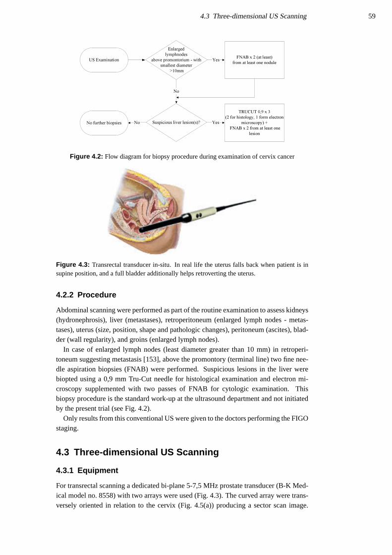
4.3 Three-dimensional US Scanning 59

FNAB x 2 (at least)

from at least one nodule

Enlarged

lymphnodes

above promontorium - with

smallest diameter

>10mm

Yes

Suspicious liver lesion(s)? Yes

TRUCUT 0,9 x 3

(2 for histology, 1 form electron

microscopy) +

FNAB x 2 from at least one

lesion

No

NoNo further biopsies

US Examination

Figure 4.2: Flow diagram for biopsy procedure during examination of cervix cancer

Figure 4.3: Transrectal transducer in-situ. In real life the uterus falls back when patient is insupine position, and a full bladder additionally helps retroverting the uterus.

4.2.2 Procedure

Abdominal scanning were performed as part of the routine examination to assess kidneys(hydronephrosis), liver (metastases), retroperitoneum (enlarged lymph nodes - metas-tases), uterus (size, position, shape and pathologic changes), peritoneum (ascites), blad-der (wall regularity), and groins (enlarged lymph nodes).

In case of enlarged lymph nodes (least diameter greater than 10 mm) in retroperi-toneum suggesting metastasis [153], above the promontory (terminal line) two fine nee-dle aspiration biopsies (FNAB) were performed. Suspicious lesions in the liver werebiopted using a 0,9 mm Tru-Cut needle for histological examination and electron mi-croscopy supplemented with two passes of FNAB for cytologic examination. Thisbiopsy procedure is the standard work-up at the ultrasound department and not initiatedby the present trial (see Fig. 4.2).

Only results from this conventional US were given to the doctors performing the FIGOstaging.

4.3 Three-dimensional US Scanning

4.3.1 Equipment

For transrectal scanning a dedicated bi-plane 5-7,5 MHz prostate transducer (B-K Med-ical model no. 8558) with two arrays were used (Fig. 4.3). The curved array were trans-versely oriented in relation to the cervix (Fig. 4.5(a)) producing a sector scan image.


(a) Motorozied ECRM unit that rotates thetransducer during acquisition.

(b) Transducer mounted in ECRM

Figure 4.4: ECRM device

(a) Image plane acquired using transverse convexarray

(b) Sweep performed by transducer mounted inECRM. The acquisition is made from -90 to

+90 degrees using the sagittal array.

Figure 4.5: Transducer and imaging planes

The linear array was sagitally oriented, producing a rectangular image (Fig. 4.5(b)) witha width of 5 cm (sagitally) and variable depth (Fig. 4.6(a)).

The same scanner used for 2D US were used for 3DUS with an add-on 3D solution(L3Di from the former Life Imaging Systems, Ontario, Canada - now provided by B-KMedical A/S). The 3D system consisted of an ordinary PC with a frame-grabber record-ing the US image on the screen of the scanner. The acquisition was controlled by theL3Di system with a so-called endocavitary rotational mover (ECRM) that controls theposition of the transducer during acquisition (see Fig 4.4).

4.3.2 Acquisition

After rectal palpation with the patient in supine position the transducer was introducedguided by the US image recorded using the transverse curved array (Fig. 4.5(a)) until thecervix was reached. Both transverse and sagittal images could be used for aligning thetransducer correctly. Correctly aligned the image using the linear array is a sagittal sliceof the cervix (Fig. 4.6(a)).

The region-of-interest was selected (Fig. 4.6(b)) and acquisition started by pushingthe button on the ECRM. By first rotating the transducer to -90 degrees and then duringacquisition to +90 degrees a half-cylinder was covered (Fig. 4.5(b)).

Three recordings were done in every case. The first aligned in the mid-sagittal plane

4.3 Three-dimensional US Scanning 61

(a) Mid-sagittal US image of Cervix using linear ar-ray. The image width was 5 cm with variable

depth.

(b) Selection of Region-of-Interest (ROI) on 2D im-age before acquisition (dotted white rectangle)

Figure 4.6: Mid-sagittal B-mode image before acquisition and selection of ROI.

Figure 4.7: Gas between trans-ducer and cervix prevents imaging.

of the cervix, the two others placed at the left and right lateral borders respectively toensure good imaging of those. This was done because edge shadows tend to obscure thelateral borders when using the mid-sagittal approach. In patients, where the cervix wasto large to be covered by one sweep (in longitudinal dimension), more acquisitions wereattempted. After acquisition image data was stored on CD-R media for later evaluation.

Air in the rectum often obscured imaging (Fig. 4.7). This was solved by letting outgas using a small silicone female urinary catheter which allowed subsequent imaging inmost cases.

4.3.3 Registration of Results

For each quadrant of the cervix (facing left and right parametrium, rectum and blad-der respectively) it was registered whether the cervix were well defined without signsof tumor extension, whether the tumor extended outside the cervix or in case of theparametrium; whether tumor had reached the pelvic wall. The findings were registeredon a schematic diagram (Fig. 4.8). Volume measurements, were done later (see Sec-tion 5.5 on page 79).

Three-dimensional ultrasound results were not allowed to induce further biopting.


Figure 4.8: Diagram used for recording tumor spread findings. By marking all the fields thatapply in the right figure the stage can be read directly from the left. The diagram was used in allmodalities: Clinical staging, 3DUS, MRI, and pathological evaluation

4.4 Clinical Staging

The clinical staging was performed according to guidelines from the International Fed-eration of Gynecology and Obstetrics (FIGO) described in Appendix A. Palpation, in-spection, colposcopy, endocervical curettage, hysteroscopy, cystoscopy, proctoscopy, in-travenous pyelography, and X-ray examination of the lungs and skeleton are allowedexaminations for the staging. Other modalities as computerized tomography (CT), MRIand US can be used for planning of treatment but not for staging. At Herlev Hospitalintravenous pyelography are substituted by ultrasound examination of the kidneys.

The main examinations cystoscopy, gynaecological examination including bi-manualvaginal and rectal palpation, and proctoscopy were done in general anesthesia in onesession at the operation theater. They were performed by one or two senior gynecolo-gists and one oncologist. Only the result from ultrasound examination of the kidneyswere available for the staging. US of liver and retroperitoneum were also available fortreatment planning.

Registration of findings were done on a diagram as described in Section 4.3.3. Thefields ”Bladder” and ”Rectum” are marked if tumor infiltration are found by cystoscopyand proctoscopy respectively. Furthermore, the size judged by inspection and palpation(in cm) were registered, as the best attainable measure of tumor volume.

If tumor masses were found descending into the vaginal wall, the rectum (proc-toscopy) or bladder (cystoscopy) surgical biopsies were taken.

4.5 MRI

To further evaluate the tumor spread, primarily in cases without a gold-standard result,that is in cases not treated with surgery, magnetic resonance imaging (MRI) was used.In addition to the evaluation done by an experienced radiologist, the volume data werecompared with US and histological results as described in Section 4.1.5.

4.5.1 Equipment and Methods

MRI was done using a closed coil 1,5 Tesla magnet (Vision, Siemens Medical, USA)with both a dedicated endorectal cervix coil (Cervix Coil-BCR, MRInnervu, MedradInc., Pittsburgh, PA, USA) and external pelvic and abdominal coils for the pelvis and

4.6 Pathological Evaluation - Gold Standard 63

Figure 4.9: Endorectal MR cervix coil

retroperitoneum. The dedicated coil (Fig. 4.9) was placed in the rectum adjacent to thecervix, unfolded and fixated by inflating a 50 ccm balloon. The coil was inserted withthe patient lying on the side, whilst the scanning is done in supine position. Both T1

and T2 weighted images were acquired before and after contrast infusion (Magnevist0,2 ml/kg).

4.5.2 Registration of Results

Results of MRI were immediately registered on the staging diagram (Fig. 4.8) togetherwith length, height, and width of tumor. In addition any enlarged lymph nodes wereregistered. As the results will show later, the planned MRI part of the study was not verysuccessful.

4.6 Pathological Evaluation - Gold Standard

Pathological examination of the cervix (operation specimen) were of course only pos-sible in cases selected for surgical treatment. Based on the histological examination ofthe specimen and (if any) biopsies, sites of cancer were determined and a TNM stage2

assigned. This TNM stage correlates directly to the FIGO stages (Appendix A).The examination of the operation specimen normally gives exact information about

depth and breadth of tumor growth from the cervical canal and about any spread intoparametrium and vagina. All lymph nodes removed during surgery are examined formetastasis. This examination are considered a ’gold standard’, that can be used to eval-uate the accuracy of US, MR and clinical examination.

The pathologist did not have access to results of US nor MRI, but clinical staginginformation could not be kept completely blinded, since pathological examination onlywill take place when operation has been performed, indicating a clinical staging belowIIB.

The preparation of the cervix was performed in a special way (see Section 4.9.5) tomake a three-dimensional reconstruction and thereby direct comparison of cancer sizeand location with US, MRI and clinical results possible. Based on the pathologicaldescription, the staging diagram (Fig. 4.8) could be filled in. Tumor volume estimateswere done as described in Section 4.9.5 and Section 5.5.

2The TNM system is a clinical staging system; where T refers to tumor size, N number and location oflymph node metastases, and M to presence and extent of distant metastases.


4.7 Blinding

The three types of examinations: 3D-TRUS, MRI and clinical examination were doneby different medical doctors without any knowledge of each others results. The pathol-ogist did not receive the clinical and para-clinical results, except for the un-maskableinformation, that the bare presence of a surgical specimen tells, that the clinical work-upresulted in a stage less than IIB. It does not, though, seem likely, that this will influencethe result. In the present trial, clinical staging was performed after US examination, sothe patient could not inadvertently inform the ultrasonographer about the findings. Nei-ther the patient nor the clinical doctors were informed about the 3DUS findings. Theresults of conization prior to ultrasound examination was not know by MHP before thefinal data analysis.

4.8 Trial Approval, Safety, and Patient Strain

The more extensive diagnostic tests performed in the present study are inherently safewithout any known adverse effects, except for the MRI contrast agent (see Section 4.8.2).Therefore it seems ethically reasonable to subject patients to this trial having the possiblebenefits in mind.

Approval of the trial by the local scientific ethical commitee of Copenhagen Countywas sought and granted: Reg. no. KA01008, 2001-03-26. All guidelines were followedand written consent was obtained from the patient after oral and written information hadbeen given.

4.8.1 Ultrasound Safety

Ultrasound scanning is regarded as a modality without adverse effects. No injuries hasbeen reported from use of US within recommended safety limits [154] for sound in-tensity. Transrectal US (TRUS) is a well-established modality for evaluation of pelvicorgans and is used on a daily bases at the Dept. of Ultrasound.

Normally, 30 minutes are allocated for scanning patients with cervical carcinoma. Theusual scan consists of transabdominal scanning (primarily of the kidneys) and transvagi-nal US scanning. The 3D-TRUS acquisition lasts approximately 10 minutes and doesnot subject the patient to any greater discomfort. It is comparable to a routine rectalexam.

4.8.2 MRI Safety

As with ultrasound scanning, MRI has been used for decades without showing any ad-verse effects, as long as the transmitted energy (RF signals) does not induce tissue dam-aging heating. The MR scanner used has built-in safety functions, that automaticallyensures that. Before MRI, the patient had to fill out a form (”Kontrolskema med henblikpa MR-scanning”, Rigshospitalet) concerning issues that could contraindicate MR scan-ning (such as metallic implants and claustrophobia). This information were verified bythe responsible doctors (MHP and a senior radiologist) with the patient present. If anycontraindications, MRI were not performed.

MR scanning took approximately 30 minutes with external pelvic coil and 20-25 min-utes with endorectal coil, with a short 5 minutes break in-between. The scanning itself is

4.9 Data Analysis 65

not associated with any pains or discomfort, but introduction of the rectal coil will oftenbe a bit uncomfortable.

Due to lacking MRI resources at Herlev Hospital, imaging was done at Rigshospitalet(Billeddiagnostisk Center). Patients were offered free transportation, and the responsi-ble investigator (MHP) met her at the reception and stayed through the whole scanningsession.

The contrast agent Magnevist (Schering) were used (dosage: 0.2 ml/kg). Nausea,vomiting, or allergic reactions can be induced3. No absolute contraindications exist.Peristaltic movements during scanning inducing imaging artifacts can be suppressed byintravenous injection of butylscopolamine (Buscopan) 20 mg IV (contra-indicated incase of narrow-angle glaucoma) or glucagon (Glucagen) 0.5-2.0 mg IV or IM (contra-indicated in case of diabetes).

4.8.3 Influence on Treatment

Patients that did not wish to participate were treated according to usual principles andguidelines. The diagnostic imaging in this project did not influence the patient’s treat-ment in any way, nor did it prolong the diagnostic work-up. Results of 3D-TRUS andMRI were not available to the clinical doctors.

4.8.4 Data Integrity and Security

Case record forms were kept by MHP in a locked office at Herlev Hospital. Other resultsfrom MRI and clinical evaluation were be kept by doctors involved in the project. Allimage data were stored on standard media (optical discs and CD-ROMs) and stored atthe departments following standard procedures or locked in at MHP’s office. All patientrelated information such as case record forms in electronic form were stored encrypted(high security 128-bit key protection) on a password protected PC. Data containing per-sonal information will be anonymized after the trial has ended.

4.9 Data Analysis

Evaluation of 3DUS stages, tumor volume, and morphology were done by MHP beforeclinical and pathological information were received from partners. Clinical information(stage and tumor spread) was noted by clinical partners on the supplied forms. Operabil-ity was decided from the assigned stage using the standard threshold (≤IIA: Operable,≥IIB: Not operable). The same FIGO criteria were used to translate the description bythe pathologist into TNM stages and operability.

4.9.1 Data Format Conversion Tool

Software dubbed ”dizVolKonvertor” was developed to convert volume data from thedifferent modalities to a common 3D format. This way data from 3DUS, MRI, andhistology could be visualized and analyzed in the same 3D program. The target formatfor the conversion format used by the Kretz 3D View 2000, which is freely available4.

3Lethal reactions have been reported - see Jordan RM, Mintz RD. Fatal reaction to gadopentetate dimeg-lumine. AJR 1995;164:743-44 including references to other cases.

4http://www.sonoportal.net


Figure 4.10: Sequelae to coniza-tion showing a well-defined hypo-echoic region located at the externalos. In this case conization changesand tumor is clearly distinguishable.

(a) Sagittal view (b) Oblique view from below

The program reads Life Imaging Systems .L3D files, Analyze5 3D files, and pure binarydata volumes. The program which also provides bi-linear interpolation and resamplingof the volume data is described in Appendix C.2. The program was used primarily todo the morphological comparison of tumors depicted by the three different modalities(3DUS, MRI, and histology).

4.9.2 3DUS Evaluation

All US volume analysis was done 9 months after last acquisition, blinded from clinicaland pathological information. This way the 3DUS results were only based on the 3Ddata without information from the contact with the patient (palpation and transvaginalscanning).

Evaluation of tumor location and spread was done using the L3Di software on anordinary PC. This program was chosen for the evaluation mainly because of its fastresponse in volume interaction and the possibility to landmark structures before volumemeasurements as discussed in Section 1.6 on page 34.

First, it was important to notice whether a conization had been performed before3DUS and when, since such a procedure can produce quite dramatic changes in the tis-sue and therefore also influence images. A case is shown in Fig. 4.10, where tumor andconization sequelae are clearly distinguishable, which is not always the case. Especiallywhen tumors are very small they can undoubtedly ’drown’ in the conization changes.Since the area of conization could be both hypo- and hyper-echoic, the distinction fromtumor was made primarily by location and difference in echogenicity.

Then the cervix was examined by moving sagittal, axial, and frontal planes in and out,especially evaluating the border of the cervix for any irregularities. This border againstthe parametria is not a well defined edge since the muscle layers of the cervix gradually’dissolves’ into the fibrous parametrial tissue. Even for the pathologist, the border be-tween cervix and parametrium can be hard to determine. Therefore, the evaluation wasprimarily concentrated on irregularities at this fictive border and on whether any visibletumor inside the cervix extended into or through this border-zone.

Evaluation of tumor growth down in the vaginal wall were not really expected to bevery visible using 3DUS, but pronounced thickening of the vagina would suggest that.Growth into bladder or rectum were to be detected as tumor masses compressing the

5ANALYZE 7.5 image file format created at the Mayo Clinic - http://www.mayo.edu/bir/


(a) Frontal view with delineated tumor (b) Frontal markings seen from side andbelow

(c) Adding sagittal delineations

(d) View from below (axial cut) showingfrontal and sagittal markings

(e) Beginning planimetry using axialplanes

(f) Result

Figure 4.11: Procedure used to measure tumor volume. First tumor was delineated in multipleplanes orthogonal (sagittal and frontal) to the plane used for planimetry (axial).

structures and disrupting the mucous membranes. Also dilated ureters should be possibleto detect in some cases. Since cervical tumors can be both hypo- and iso-echoic, no rigidcriteria about echogenicity could be applied.

4.9.3 3DUS volume Measurements

Tumor volume was measured using planimetry. As described in Section 1.6 on page 34it is necessary to examine the tumor with intersecting planes of different orientation, andto mark features found in other plane orientations for use as landmarks during planime-try. Therefore, tumor outlines were made in sagittal and frontal slices before the finalplanimetry was performed using axial planes (Fig. 4.11). If other oblique planes weremore relevant, better depicting the tumor, they were used for marking before planime-try. For instance a plane orthogonal to the plane dividing two structures (cervix andparametrium) is more relevant to use than a strict anatomical frontal plane. The volumeof the whole cervix was also measured, by first marking the internal os using two or morelines orthogonal to the cervical canal. In many cases, though, deformation from tumorand a cervix size superseding the volume covered by the sweep, made such a volumeestimation seem unrealistic.

4.9.4 MRI Evaluation

Since very few patients underwent MRI in this trial (see Chapter 5 Results) no stan-dard scheme for evaluating MRI images was applied. Instead the reconstructed three-dimensional volumes were compared with 3DUS and reconstructed histology volumes


Figure 4.12: Cutting procedure used to make histologic slides.

side by side.

4.9.5 Assembling Histological Slices

The surgical specimen usually consist of the uterus in toto, parametria, top part of vagina,and resected pelvic lymph nodes.

For preparation the uterus was cut in a transaxial plane at the level of the internalorifice (the narrowest location between cervix and the uteral body). This level’s distancefrom the external orifice in centimeters was recorded. Then the cervix was fixated. Afterfixation the cervix was cut in transaxial slices with a distance of 5 mm (in some cases10 mm). The resulting slices were divided by a frontal plane in anterior and posteriorparts, which then again was cut by sagittal planes to make the tissue samples fit thehistological glass slides (Fig. 4.12).

On all histological slides the pathologist marked the border of the cervix and cancertissue. Then all slides were scanned using a flatbed scanner at a resolution of 600 dotsper inch. The full planes were assembled for each 5 mm like a puzzle using Adobe Pho-toshop v7.06 (Fig. 4.13), which allowed visually guided rotation and translation of theparts making up a full section. Histological slices with a 5 mm inter-distance provided aspatial resolution far from the ideal isotropic7 one. Scanning slides using a microscopeat a µm in-plane resolution would therefore be overkill. The difference in resolutionwould be around three orders of a magnitude. Small alignment errors (1-2 mm) arisingwhen manually stitching together the individual slide pieces in the puzzle are thereforenot significant either; firstly because deformation of tissue during fixation often is larger,secondly, because the modalities to compare with (ultrasound, MR, and clinical exami-nation) all have less effective accuracy. By effective accuracy is meant that even thoughUS often have sub-millimeter resolution, variation in sound speeds in different tissue,

6http://www.adobe.com7Isotropic means invariant with direction. With respect to resolution it means that the resolution is the

same in all directions, i.e. the three dimensions


Figure 4.13: Five microscopic transaxial slices assembled into two full cervical slices at twodifferent heights (centimeters from external orifice). The red lines delineate the cervix wall, theblack indicate the outer border of cancer tissue (drawn by pathologist). The inner edge of thelines indicate the border. Slices are seen from above (superior to inferior) and left side in thepicture is the patients left side. The ’cm’ annotation is distance to external os.

diffraction, and reflection of the sound mean that the absolute position of an image pointcannot be mapped to real world coordinates with sub-millimeter precision. Therefore,the precision achieved by scanning slides at 600 DPI (236.2 points/cm) and manual stack-ing of assembled puzzles from the different levels would be sufficiently accurate forcomparing tumor size, location, and outgrowth from cervix to the other modalities. Af-ter assembly the image was subsampled to a 50 pixels/cm resolution for further processing.

The delineations of tumor and cervix were traced using NIH Image to measure theareas at each level. Volumes (V ) were estimating by adding the product of area (A) andslice distance (d) at each level:

V =n

∑1

A ·d. (4.1)

To reconstruct volume data images of each level were stacked and converted to grayscale using ImageJ8. Subsequently images in the stack were aligned (registration) usingNIH Image9. A small program using the Scion Image macro language was written toperform the alignment process. In every slice of the stack the line dividing the anteriorand posterior part of the cervix was delineated. Since the cervix was cut by this frontalplane before further division, this is a robust marker to be used for registration. Fur-thermore the center (the cervical canal) was pointed out by moving the line ROI withoutchanging the angle - especially in cases where the initial line marked was off center.After having indicated this line manually the macro translated and rotated the each sliceindividually (see Fig. 4.14).

Conversion from the image stack to the Kretz file format using the dizVolKonvertortool included re-sampling of the volume to isotropic resolution needed by the Kretzsoftware. This involves three-dimensional bilinear interpolation. Since the differencebetween the original slices with a distance of 5 or 10 mm is considerable, each slice

8Image processing toolbox developed at Research Services Branch National, National Institute Health,USA - Freely available for multiple platforms at http://rsb.info.nih.gov/ij/

9Image processing tool, developed by Wayne Rasband at NIH for the Macintosh platform:http://rsb.info.nih.gov/nih-image/. A port for the Windows platform has been made by Scion Coop-eration, freely available from http://www.scioncorp.com/


(a) Slices with 5 mm between, which are not aligned for stacking. Marked by fiducial point for registration.

(b) After registration where slices are centered and rotated.

Figure 4.14: Slices before and after alignment. Notice, that slice 5 and 7 are repeated, since thedistances between the pairs 5-7 and 7-9 are 1 cm.

were replicated 5 or 10 times for the 5 and 10 mm slice distances respectively. That waya stack consisting of solid slabs with 1 mm thick interpolation zones in between wascreated. The volumes were re-sampled to cubic voxels with 0.3 mm sides.

71

Chapter 5

Results

I know why there are so many peoplewho love chopping wood.

In this activity one immediately sees theresults.

Albert Einstein

Contents5.1 3DUS Imaging . . . . . . . . . . . . . . . . . . . . . . . . . . . . 725.2 Comparison between 3DUS and Clinical Staging . . . . . . . . . 745.3 Comparing to Histology Results . . . . . . . . . . . . . . . . . . 785.4 Imaging after Conization . . . . . . . . . . . . . . . . . . . . . . 785.5 Tumor Volume . . . . . . . . . . . . . . . . . . . . . . . . . . . . 795.6 Tumor Location Comparison . . . . . . . . . . . . . . . . . . . . 815.7 MRI Results . . . . . . . . . . . . . . . . . . . . . . . . . . . . . 825.8 Comparison of Tumor Morphology . . . . . . . . . . . . . . . . 835.9 Addendum - Case Story . . . . . . . . . . . . . . . . . . . . . . . 84

53 consecutive patients fulfilling the inclusion criteria were referred for treatment dur-ing the inclusion period (June 2001 to March 2002 interrupted by a 3 weeks vacation).This was less than the 75 expected for 3/4 year1. Only 23 were willing to participate, 3were subsequently excluded resulting in a total of 20 participants. The mean age was

1The duration was changed to allow completion of internship

Age Distribution

Age [years]

Fre

quen

cy

30 40 50 60 70 80

01

23

45

67

−2 −1 0 1 2

3040

5060

7080

Normality Plot

Theoretical Quantiles

Sam

ple

Qua

ntile

s

Figure 5.1: Distribution of ages of participating patients

72 Chapter 5 Results

(a) Ovarian tumor (b) Uteral body tumor

Figure 5.2: Ovarian and uteral body tumor in the excluded patients 10 and 13.

53.1 years (range 30.5 to 78.3 - see distribution on Fig. 5.1), which is not noticeabledifferent from the demographic data presented in Section 3.1.

Of the participating patients only 5 were willing to undergo MR imaging. One of thosesuffered so much from claustrophobia that MRI was impossible, another so that only anopen coil magnet could be used, in which transrectal MRI was not possible. Technicalproblems and an emergency scanning prevented transrectal scanning in the two othercases. On that basis we refrained from transrectal MRI in the last patient. To conclude,MRI scanning was not successful and can therefore not be used for staging comparison.The few scans performed will be described on a casuistic basis in Section 5.7.

Staging and operability results from 3DUS, clinical staging, and histological exami-nations are listed in Table 5.1.

Patients no. 7, 10, and 13 were excluded. Patient 7 was excluded due to exclusioncriterium no. 4 (see Section 4.1.3 on page 57). The conization performed before 3DUSshowed stage IA1 and subsequent re-conization revealed no remaining tumor tissue.Patient no. 10 had a large ovarian tumor visualized by ultrasound and also determinedby clinical staging (Fig. 5.2(a)). 3DUS of patient no. 13 showed a large tumor extendinginto the body of the uterus which was heavily deformed (Fig. 5.2(b)). This turned out tobe a corporal cancer.

5.1 3DUS Imaging

In all cases 3DUS was possible to carry through. But in two patients (no. 8 and 9)results were inconclusive because of abundant air in the rectum yielding volumes withso heavy acoustic shadowing that evaluation was not possible. This problem was solvedfor the following patients using the method described in Section 4.3.2. The image qualityand volume coverage was generally better in women with retroverted uteruses and withfull bladders, which induce retroversion. This provided a better contact between thetransducer and the posterior wall of the cervix, whereas an anteverted cervix turns theinferior part with the external os against the transducer - an inferior surface which isoften uneven due to tumor growth or conization sequelae. This uneven surface can havesmall air pockets obscuring cervical structures.

In the remaining patients, 3DUS image (volume) quality was suitable for diagnosticdecisions, as the examples shown in Fig. 5.5. In a few cases, though, the staging decision

5.1 3DUS Imaging 73

Tab

le5.

1:R

esul

tsof

3DU

S,E

GA

,and

path

olog

ical

stag

ing.

Patie

ntA

geC

onis

.3D

US

EG

ASu

rger

yH

isto

logy

no.

befo

reSt

age

>4

cmSc

ale

Ope

rabl

eSt

age

>4

cmSc

ale

Ope

rabl

epe

rfor

med

Stag

e‡>

4cm

Scal

eO

pera

ble

152

,6Y

es2B

Yes

5N

o3B

Yes

7N

oN

o-

--

-2

36,4

Yes

1B1

No

2Y

es1B

1N

o2

Yes

Yes

1B1

No

2Y

es3

32,4

No

1B1

No

2Y

es1B

2Y

es3

Yes

Yes

1A2

No

1Y

es4

53,8

No

2BY

es5

No

2BY

es5

No

No

--

--

565

,8Y

es1A

No

1Y

es1B

1N

o2

Yes

Yes

1B1

/N

o2

/1Y

es6

33,9

No

1B1

No

2Y

es1B

1N

o2

Yes

Yes

1B1

No

2Y

es8

57,2

No

††

††

2AN

o4

Yes

Yes

2BN

o5

No

952

,9N

o†

††

†3B

-7

No

No

--

--

1172

,2N

o2B

No

5N

o1B

1N

o2

Yes

Yes

2BN

o5

No

1278

,2N

o3B

Yes

7N

o1B

1N

o2

Yes

No

--

--

1448

,8Y

es1B

1N

o2

Yes

1B1

No

2Y

esY

es1B

1N

o2

Yes

1554

,4Y

es1B

1N

o2

Yes

1B1

No

2Y

esY

es1B

1N

o2

Yes

1665

,4N

o2B

No

5N

o2B

No

5N

oN

o-

--

-17

30,5

Yes

1AN

o1

Yes

1B1

No

2Y

esC

onis

.1B

1/1

A1

2/1

Yes

1856

,5Y

es1B

1N

o2

Yes

1AN

o1

Yes

Yes

1A/

No

1Y

es19

78,3

No

2BN

o5

No

2BN

o5

No

No

--

--

2058

,8N

o1B

1N

o2

Yes

2BN

o5

No

No

--

--

2134

,8N

o1B

1N

o2

Yes

1B1

No

2Y

esY

es1B

1N

o2

Yes

2269

,0N

o4A

No

8N

o3B

-7

No

No

--

--

2345

,1N

o2B

Yes

5N

o3B

Yes

7N

oN

o-

--

-

†:3D

US

notp

ossi

ble

beca

use

ofab

unda

ntga

s‡:

Ass

igne

dst

age

/Pse

udo-

stag

eaf

ter

3DU

San

dop

erat

ion

orre

-kon

isat

ion

:

No

canc

er-

:N

otav

aila

ble


(a) Retroverted uterus with a filled bladder provid-ing good transrectal image quality

(b) Anteverted uterus with empty bladder result-ing in low quality image due to shadowing

Figure 5.3: Effect of uterus retro- and anteversion on image quality

(a) Transaxial view. Large tumor seen onright side.

(b) Combined frontal and sagittal view. (c) Sagittal view.

Figure 5.4: Large hyper-echoic homogenous tumor in right side of parametrium, either stageIIIB cervical , uteral body, or ovarian tumor (patient no. 12).

was more difficult. The 3DUS of patient number 5 could not depict any tumor butthe left border of the cervix against the parametrium was somewhat irregular whichcould indicate tumor outgrowth, if the cervix were infiltrated with tumor not visible onultrasound (Fig. 5.6 and 5.7). The area was interpreted as not being tumor tissue. Almostthe same was the case in patient number 6, except that tumor tissue could be visualizedinside the cervix (Fig. 5.8 and 5.9). The suspicious area in the cervix against the leftparametrium was in that case clearly different in echogenicity from the visible tumormass. Histologic examination revealed endometriosis at that location.

Images of patient no. 12 showed a big at least 7×7×5 cm sized hyper-echoic tumorextending from the right upper side of the cervix representing either a stage IIIB or morelikely an ovarian or uteral body tumor. Comparing the images (Fig. 5.4) to the onesshown in Fig. 5.2 indicated an uteral body tumor.

5.2 Comparison between 3DUS and Clinical Staging

Table 5.2 shows results sorted by increasing clinical stage. The operability results showdisagreement between clinical stage and 3DUS results in three (no. 11, 12, and 20) out

5.2 Comparison between 3DUS and Clinical Staging 75

(a) Tumor invading right parametrium (IIB) (b) Extending into left parametrium (IIB) (c) Tumor mass encasing leftureter just beneath themucous membrane of the

bladder.

(d) Frontal view of tumor extending superiorly intoleft parametrium

(e) Tumor extending into left parametrium,staged to IIIB by EGA (IIB by 3DUS)

(f) Tumor mass nudging therectal wall but not disrupt-ing the layers of the rectum

Figure 5.5: Image examples

Table 5.2: Results of 3DUS, EGA, and pathological staging ordered by measurement parameterand sorted by EGA result. The arrows indicate staging differences between EGA and 3DUS.

Patient Stage Ranked Scale > 4 cm OperableNo. EGA 3DUS Hist. EGA 3DUS Hist. EGA 3DUS Hist. EGA 3DUS Hist. Surgery17 1a1 ↔ 1a 1a1 1 ↔ 1 1 0 ↔ 0 0 1 ↔ 1 1 Conis.18 1a1 ↗ 1b1 0 1 ↗ 2 0 0 ↔ 0 0 1 ↔ 1 1 15 1b1↖ 1a 0 2 ↖ 1 0 0 ↔ 0 0 1 ↔ 1 1 12 1b1↔ 1b1 1b1 2 ↔ 2 2 0 ↔ 0 0 1 ↔ 1 1 16 1b1↔ 1b1 1b1 2 ↔ 2 2 0 ↔ 0 0 1 ↔ 1 1 114 1b1↔ 1b1 1b1 2 ↔ 2 2 0 ↔ 0 0 1 ↔ 1 1 115 1b1↔ 1b1 1b1 2 ↔ 2 2 0 ↔ 0 0 1 ↔ 1 1 121 1b1↔ 1b1 1b1 2 ↔ 2 2 0 ↔ 0 0 1 ↔ 1 1 111 1b1↗ 2b 2b 2 ↗ 5 5 0 ↔ 0 0 1 ↗ 0 0 112 1b1↗ 3b ‡ 2 ↗ 7 ‡ 0 ↗ 1 ‡ 1 ↗ 0 ‡ ‡3 1b2↖ 1b1 1a2 3 ↖ 2 1 1 ↖ 0 0 1 ↔ 1 1 18 2a † 2b 4 † 5 0 † 0 1 † 0 120 2b ↖ 1b1 - 5 ↖ 2 - 0 ↔ 0 - 0 ↖ 1 - 04 2b ↔ 2b - 5 ↔ 5 - 1 ↔ 1 - 0 ↔ 0 - 016 2b ↔ 2b - 5 ↔ 5 - 0 ↔ 0 - 0 ↔ 0 - 019 2b ↔ 2b - 5 ↔ 5 - 0 ↔ 0 - 0 ↔ 0 - 022 3b ↗ 4a - 7 ↗ 8 - - 1 - 0 ↔ 0 - 09 3b † - 7 † - - † - 0 † - 01 3b ↖ 2b - 7 ↖ 5 - 1 ↔ 1 - 0 ↔ 0 - 023 3b ↖ 2b - 7 ↖ 5 - 1 ↔ 1 - 0 ↔ 0 - 0†: 3DUS not possible because of abundant gas. : No cancer‡: This patient was not operated because of her age (78)


Figure 5.6: Frontal view of irregular iso-echoic struc-ture at left brim of cervix (patient 5).

Figure 5.7: Same region in transaxial view.

Figure 5.8: Transaxial view of cervix with hyper-echoic irregular structure at left side (patient 6).

Figure 5.9: Same cervix in frontal view, showing samehyper-echoic structure at left border of cervix againstleft parametrium.

5.3 Comparing to Histology Results 77

of the remaining 20 patients - two with a clinical stage indicating operability and onejudged as non-operable. The very low number of patients makes statistical analysisalmost superfluous. The two cases without a 3DUS result (ptt. 8 and 9) should be treatedas cases where 3DUS are ’wrong’ i.e. no agreement, even though most of such non-informative answers presumably can be avoided in the future. The degree of agreementcan be described using the Cohen kappa (κ) measure[155]2. The resulting kappa value(0.49) is generally interpreted as moderate strength of agreement, with a confidenceinterval from poor to very good (Table 5.3). Agreement on operability could potentially

3DUS Kappa StatisticsEUA No Yes Kappa 0.490

No 6 1+1 C.I. lower 0.103Yes 2+1 9 C.I. upper 0.877

Table 5.3: Comparison of operabilityjudged by clinical staging (EGA) and3DUS.

hide disagreement on staging below or above the operation threshold. From the resultsin Table 5.2 we can see that the actual assigned stage differs from 3DUS result in 6 outof the 15 cases with operability agreement.

Comparing the actual stages assigned by EGA and 3DUS (Table 5.4) reveals furtherdisagreement described as ’fair’ using the un-weighted kappa measure, with a confidenceinterval ranging from ’poor’ to ’good’. In this calculation the two cases without 3DUSresults were not included, since it makes no meaning to assign some arbitrary stagefor those. The kappa value calculated without weighting is artificially low, since theassigned stages might correlate even if they are not exactly the same. The FIGO scalecan be considered as a ranked scale clinically i.e. higher stage - more severe disease.Imaging wise, this approximation is not ideal for method comparison. For instancestages IIIA and IVA are closer morphologically than IIIA and IIIB are. This problemwill be dealt with in Section 5.6 on page 81. Therefore, the ranked scale approach seemsunfair to the diagnostic modalities. No general over- or under-staging bias could bedetected. 3DUS yield a higher stage than EGA in 4 cases and lower in 5.

Table 5.4: Comparison of staging results between EGA and 3DUS.

3DUSEUA 1: IA 2:IB1 3:IB2 4:IIA 5:IIB 6:IIIA 7:IIIB 8:IVA Total Kappa Statistics1: IA 1 1 0 0 0 0 0 0 3 Kappa u.w. 0.2932:IB1 1 5 0 0 1 0 1 0 8 C.I. Lower -0.033:IB2 0 1 0 0 0 0 0 0 1 C.I. Upper 0.6194:IIA 0 0 0 0 0 0 0 0 05:IIB 0 1 0 0 3 0 0 0 4 Kappa w. 0.5216:IIIA 0 0 0 0 0 0 0 0 0 C.I. Lower -0.0167:IIIB 0 0 0 0 2 0 0 1 3 C.I. Upper 1.0588:IVA 0 0 0 0 0 0 0 0 0Total 3 8 0 0 6 0 1 1 19


Table 5.5: Results of 3DUS, EGA, and pathological staging shown only for patients with histo-logical results. Sorted by histological result. The arrows indicate over- (↑) and understaging (↓)compared to histologic result.

Patient Stage Ranked Scale Operability SurgeryNo. Histol. EGA 3DUS Histol. EGA 3DUS Histol. EGA 3DUS18 0 1a1↑ 1b1↑ 1 1 2↑ 1 1 1 15 0 1b1↑ 1a↑ 1 2↑ 1 1 1 1 117 1a1 1a1 1a 1 1 1 1 1 1 Conis.3 1a2 1b2↑ 1b1↑ 1 3↑ 2↑ 1 1 1 12 1b1 1b1 1b1 2 2 2 1 1 1 16 1b1 1b1 1b1 2 2 2 1 1 1 114 1b1 1b1 1b1 2 2 2 1 1 1 115 1b1 1b1 1b1 2 2 2 1 1 1 121 1b1 1b1 1b1 2 2 2 1 1 1 111 2b 1b1↓ 2b 5 2↓ 5 0 1↓ 0 18 2b 2a↓ † 5 4↓ † 0 1↓ † 1

†: 3DUS not possible because of abundant gas. : No cancer found

5.3 Comparing to Histology Results

In 12 of the 23 patients (52%) a histological result was available for comparison (seeTable 5.5). In three patients (no. 5, 7 and 18) there was no cancer tissue present in thesurgical specimen, since it was removed by the preceding conization procedure. Theclinical stage assigned reflects that, since it is based partly on the conization result in ad-dition to the gynecologic examination performed to rule out additional tumor extension.The 3DUS staging was done without knowledge of the conization result.

Patient no. 7 had a IA1 tumor, did therefore not meet the inclusion criteria, and wassubsequently excluded. The 3DUS assigned stage IA since there were no no visibletumor mass.

Patient no. 5 had a IB tumor (14×8 mm) based on the conization done before re-ferral to Herlev Hospital and was therefore operated. The operation did not show anyremaining tumor, as well as the 3DUS examination. The FIGO staging was based on thatinformation, whereas the 3DUS examination based solely on the scanning result couldnot reveal the excised tumor.

Patient no. 18 was operated at her own request - ”to get it over with”. This decisionwas based partly on her age and supported by the results of the initial conization showingpronounced inflammation making it impossible to discern between stage IA1 and IA2.

If we look at the remaining patients both EGA and 3DUS overstaged patient no. 3,EGA one stage higher than 3DUS. In two patients (8 and 11) EGA understaged com-pared to histology, where 3DUS did correctly in one (no. 11), but was not possible dueto air (equalling ’wrong’) in the other (no. 8).

5.4 Imaging after Conization

Conization clearly affects the image results as shown in Fig. 4.10 on page 66. In thisexample the tumor was so clearly visible that conization changes and tumor could beseparated. In cases with much smaller tumors (<5 mm), this usually not the case. Firstly,

2For an explanation of κ see Appendix B on page 145.

5.5 Tumor Volume 79

Table 5.6: Volume measurements sorted by FIGO stage.

Patient Stage Tumor Cervixno. EGA 3DUS Histology EGA 3DUS Histology 3DUS Histology

FIGO TNM >4 cm [ml] [ml] [ml] [ml]18 1a1 1b1 0 8,1 0 14,7 12,817 1a1 1a 1a1 0 0 0,001 12,2 Conis.12 1b1 3b - 0 ‡ - ‡ -5 1b1 1a 0 0 0 3,7 4,62 1b1 1b1 1b1 0 5,5 5,18 25,6 22,86 1b1 1b1 1b1 0 † 1,2 8,6 27,514 1b1 1b1 1b1 0 2,1 0,135 26,5 42,715 1b1 1b1 1b1 0 4,9 12,6 4,6 25,521 1b1 1b1 1b1 0 † 6,06 13,5 34,311 1b1 2b 2b 0 12,5 9,66 10,1 20,63 1b2 1b1 1a2 1 † 0,19 25,7 23,18 2a × 2b 0 × 21,4 × 39,720 2b 1b1 - 0 12,1 - 18,2 -4 2b 2b - 1 † - 64,7 -16 2b 2b - 0 ‡ - 25,7 -19 2b 2b - 0 † - 2,5 -9 3b × - - × - × -1 3b 2b - 1 ‡ - 25,8 -23 3b 2b - 1 † - 18 -22 3b 4a - - ‡ - ‡ -

† Tumor not discernable from cervix No cancer found‡ Unconfined tumor - Histologic information not available× 3DUS impossible EGA >4 cm ∼ tumor volume > 33.5 cm3

because the conization procedure deliberately will partly or fully remove the tumor tis-sue. In patient no. 5 a IB1 tumor was fully removed by the procedure, and in patientno. 17 a IB1 tumor was almost removed leaving only a 1 mm2 tumor area behind (basedon histologic examination). Seven of the 20 patients had undergone conization before3DUS.

5.5 Tumor Volume

Of the 18 patients in which sufficient 3DUS imaging were achieved, tumor and cervixtissue could not be discerned clearly in 6, tumor volume estimates were made in 8, andthe tumor was unconfined in 4 cases (Table 5.6). The two cases with a 3DUS volumeestimate of 0 cm3, histologic examination did not find any tumor in one (5) and verylittle (0.001 ml) in the other (pt. 17).

Agreements between ultrasonic and histologic cervix and tumor volume measure-ments are depicted in Figs 5.10(a) and 5.10(b) on the following page respectively. 3DUSseems to underestimate the cervix volume compared to histologic result. The tumor vol-ume measurements do not show the same tendency, but the number of results are clearlyinadequate for any clear evidence. Swelling during histologic preparation or stretchingof microtome sliced specimens could cause an increased volume estimation. Since thecervical boundary against the parametria allegedly is difficult to delineate by microscopy,this could be another explanation for this difference. Finally, a bias from an erroneousassembling of the scanned slides could be the reason. All these possibilities indicate thatfurther research of this topic is required. Volumes of tumor and cervix found by 3DUS


(a) 3DUS cervix volume against histologic. (b) 3DUS tumor volume against histologic.

(c) 3DUS cervix volume against stage scale. (d) Histologic cervix volume against stage scale.

(e) 3DUS tumor volume against stage scale. (f) Histologic tumor volume against stage scale.

Figure 5.10: Cervix and tumor volumes estimated using 3DUS and histology. ”Scale” is theranked scale defined in Table 4.1 on page 58 representing the FIGO staging result.

5.6 Tumor Location Comparison 81

Table 5.7: Comparison of tumor location between 3DUS, clinical (EGA), and histologic stag-ing. A colored field indicates tumor present at that location. IIB, IIIB: Parametrial involvement.IIA, IIIA: Vaginal involvement.

Pat

ien

t

Co

niz

atio

n

Method IIIB

dxt

.

IIB d

xt

IB IIB s

in.

IIIB

sin

.

IIA IIIA

IVA

bla

dd

er

IVA

rec

tum

Sta

ge

3DUS IIBEGA IIIB

Histology

3DUS IB1EGA IB1

Histology IB1

3DUS IB1EGA IB2

Histology IA2

3DUS IIBEGA IIB

Histology

3DUS IAEGA IB1

Histology IB1 / 0

3DUS IB1EGA IB1

Histology IB1

3DUSEGA IIA

Histology IIB

3DUSEGA IIIB

Histology

3DUS IIBEGA IB1

Histology IIB

3DUS IIIBEGA IB1

Histology12

9

5

6

8

11

1

2

3

4

X

X

X

Pat

ien

t

Co

niz

atio

n

Method IIIB

dxt

.

IIB d

xt

IB IIB s

in.

IIIB

sin

.

IIA IIIA

IVA

bla

dd

er

IVA

rec

tum

Sta

ge

3DUS IB1EGA IB1

Histology IB1

3DUS IB1EGA IB1

Histology IB1

3DUS IIBEGA IIB

Histology

3DUS IAEGA IB1

Histology IB1 / IA1

3DUS IB1EGA IA

Histology 1A / 0

3DUS IIBEGA IIB

Histology

3DUS IB1EGA IIB

Histology

3DUS IB1EGA IB1

Histology IB1

3DUS IVAEGA IIIB

Histology

3DUS IIBEGA IIIB

Histology23

18

19

20

21

15

16

17

22

14 X

X

X

X

and histologic measurements versus FIGO stages are plotted in Figs. 5.10(c) to 5.10(f)on the preceding page.

5.6 Tumor Location Comparison

As mentioned in Section 5.2 the Cohen κ measure may be an inadequate comparisonmethod for the staging based on the FIGO criteria. In Table 5.7 the tumor locationsfound by the three different modalities (clinical examination, ultrasound, and histology)are depicted for each patient. Full agreement between EGA and 3DUS exists in 9 of 20cases, between 3DUS and histology in 9, and between EGA and histology in 6 cases.

In Table 5.8 the two-by-two agreement tables between the three modalities for eachlocation are depicted. The number of comparisons are clearly insufficient in most casesfor any statistical implications. The two comparisons between EGA and 3DUS of leftand right parametrium (IIB sin. et dxt.) are the only ones, where kappa values giveany meaning. For right parametrium it is κ = 0.68 c.i. [0.26-1.1] and for left κ = 0.64c.i. [0.27-1.0]. This is ’good’ agreement, but clearly the number of cases is insufficient.Comparison with histologic results cannot be done statistically with such sparse materialbut only on a casuistic basis. It is, however, interesting that 3DUS does fully agree with


Table 5.8: Agreement between modalities on location of tumor infiltration. †: Insufficient datafor κappa calculations. §: Confidence interval 0.26-1.1. ‡: Confidence interval 0.27-1.0. Seetext for further explanation.

IIIB dxt. IIB dxt. IB IIB sin. IIIB sin. IIA IIIA IVA blad. IVA rect.EGA 3DUS 3DUS 3DUS 3DUS 3DUS 3DUS 3DUS 3DUS 3DUS

Yes No Yes No Yes No Yes No Yes No Yes No Yes No Yes No Yes NoYes 1 3 1 16 2 5 2 3 2 1No 1 16 1 13 1 10 15 16 17 1 17 18

† κ:0.68 § † κ:0.64 ‡ † † † † †Histology 3DUS 3DUS 3DUS 3DUS 3DUS 3DUS 3DUS 3DUS 3DUS

Yes No Yes No Yes No Yes No Yes No Yes No Yes No Yes No Yes NoYes 6 2 1No 10 10 2 9 10 10 10 10 10

† † † † † † † † †Histology EGA EGA EGA EGA EGA EGA EGA EGA EGA

Yes No Yes No Yes No Yes No Yes No Yes No Yes No Yes No Yes NoYes 9 2No 11 11 2 9 11 1 10 11 11 11

† † † † † † † † †

histology in this distinction between IB and IIB in all cases, whereas EGA actually hastwo under-staged patients (Table 5.8).

If we only look at cases where all three kinds of data exist (10 cases), 3DUS, clinicalstaging, and histologic staging agrees in 5 (ptt. 1, 6, 14, 15, and 21 - Table 5.7). Patient 3with a histologic staging IA2 was over-staged by both 3DUS (IB1) and EGA (IB2). Pa-tient 5 with histologic staging IB1 was under-staged by 3DUS (IA), since all tumor masswas removed by conization prior to US examination (confirmed by histology). Almostthe same was the case with patient 17, where a IB1 tumor was de-bulked by the diag-nostic conization procedure before 3DUS, which rated it as IA1, which corresponded tothe remaining tumor tissue in the surgical specimen examined by histological examina-tion. Patient 18 was rated IB1 by ultrasound. The conization result and basis for clinicalstaging described a IA tumor, that could not be clearly distinguished between IA1 andIA2 due to extended inflammation. Histologic examination of the cervical specimenafter surgery showed that no tumor tissue was left after conization. In patient 11, clini-cal staging (IB1) missed left parametrial infiltration (IIB) properly detected with 3DUS.Vaginal involvement was not detected by 3DUS in any of the 4 cases detected by EGA.Two of those were the cases, where 3DUS was not successful due to air in the rectum.This might suggest, that vaginal involvement could impair 3DUS imaging. In patient 22bladder involvement was described by 3DUS (Fig. 5.5(c) on page 75). EGA (includingcystoscopy) did find bullous edema in the bladder but no invasion into mucosa, which isrequired for stage IVA. This distinction tumor just below the mucosa and disrupting themucous membrame, seems a difficult to make by ultrasound. In some cases, the decisionis a more clear cut (Fig. 5.11 - a pilot scanning, not part of the trial).

5.7 MRI Results

Not in a single case MRI using the endorectal coil succeeded. Therefore the desiredimage resolution was not achieved, limiting the possibility to do side-by-side comparisonof three-dimensional acquisitions.

5.8 Comparison of Tumor Morphology 83

(a) Tumor invading bladder. Cervixis seen in the lower left part,vagina in right, and bladder in the

upper part of image.

(b) Site where tumor extends from cervix(lower part) into bladder (upper).

(c) Sagittal view of cervix (lower left) and bladder(upper) with tumor infiltrated wall.

Figure 5.11: Large tumor invading bladder.

The resulting images made using external abdominal and pelvic coils suffered likemost clinical MR images from pronounced anisotropic resolution, i.e. an in-plane res-olution several times higher than the slice thickness. This makes the volume data lesssuitable for three-dimensional visualization and diagnostics (Fig. 5.12). MRI staging

Figure 5.12: MRI example. T2

weighted image with an in-planepixel resolution of (1.4 mm)2 and aslice thickness of 9.6 mm. The up-per left image is the acquired sagit-tal image, whereas the others arereconstructed frontal and transaxialplanes. (Patient no. 2)

results are not reported, since the low number of participants (a total of 5) were insuffi-cient to make a reasonable evaluation. The images that were acquired were compared to3DUS and histological volumes in Section 5.8.

5.8 Comparison of Tumor Morphology

The available programs (B-K Medical L3Di Viewer and Kretz 3DView 2000) could notvisualize several volumes at the same time, to align them and make a direct compari-son. Instead three instances of the program (3DView) were launched simultaneously tocompare by toggling between them (Fig. 5.13). Since the comparison of tumor locationsof staging importance and the volume estimation comparison have already been dealtwith in Section 5.6, this section will concentrate on the appearance of the tumor in eachthree-dimensional imaging modality (US, MRI, and 3D reconstructed histologic slices).Table 5.9 gives short descriptions and summaries of the visualized volumes. The tablealso contains and index to the corresponding figures on the following pages.


Figure 5.13: 3DUS, MRI, and histologic volume comparison.

Some of the cases do show full agreement between 3DUS and histology. In somecases the tumor was too small to be seen on ultrasound. Especially a prior conization issuspected to impair the visualization of small tumor. In one case (patient no. 3) whereconization had not been performed, a 0.5 ml tumor in the distal part of the cervix was notdetected. The lesion could be recognized on ultrasound images after obtaining histologicknowledge, but whether detection without that would be possible is doubtful.

5.9 Addendum - Case Story

Just before printing this thesis the following information concerning patient no. 12 wasdiscovered. A revision of the endocervical curettage had been performed changing thediagnosis to uteral body tumor (squamous cellular carcinoma). Hysterectomy was per-formed revealing an enlarged uterus (10× 10 cm), with tumor penetration of posteriorwall with rectal wall adherence i.e. uteral body cancer stage III. Radical surgery wasnot possible, and the patient died 5 months after trial inclusion having received radia-tion therapy (50 Gy). These findings confirms the suspicion of a non-cervical cancerdescribed in Section 5.1.

5.9 Addendum - Case Story 85

Table 5.9: Comparison of tumor visualization with US, MRI, and histologic volume data fromdifferent patients.

No. 3DUS MRI Histology Conclusion Figures

2 Clearly defined tumor distinctfrom surroundings containedwithin cervix.

Barely seen on bothT1 and T2 weightedimages. Only visiblewhen knowing 3DUSand histologic results

Regular shaped tumorlimited to cervix < 4 cm

3DUS detects tumor andextension in good correlationwith histologic result

Fig. 5.14to 5.16 onthe followingpage

3 Tumor not visible, but smallhypoechoic region can befound guided by histologicresult.

Tumor not visible Homogenous cervixwith small 1× 0.5 cmtumor

MRI nor ultrasound coulddetect tumor

Fig. 5.17to 5.19 onpage 87

6 Irregular 1× 1.7 cm ’scar’ indistal center (no conization)

n.a. Small 1 cm3 tumor indistal center

Similar histology and 3DUSfindings

Not shown

11 Large tumor infiltratingwhole cervix with irregularlower left border and with leftparametrial invasion

n.a. Same as 3DUS result 3DUS and histology agreefully, with parametrial inva-sion not detected by clinicalevaluation


14 Small tumor in central part2 ml

n.a. Very small tumor0.135 ml, changesinterpreted as result ofconization resemblesvolume falsely detectedas tumor with 3DUS.

Tumor found at same lo-cation, but 3DUS probablydetected conization changes


15 Relatively large well delin-eated tumor filling almostentire cervix but withoutexternal spread.

n.a. Confirms 3DUS find-ings

Full agreement between3DUS and histology


18 Irregular cervix tissue inter-preted as tumor infiltration

No visible tumor tissue Surgical specimenwithout tumor tissue butreaction to conization.

No tumor left after coniza-tion showing IA1, but in-flammation may have led to3DUS misinterpretation.


21 Major part of cervix infil-trated by tumor, no clearlimits visible but no suspicionof spread

Cervix fully in-filtrated by tumor,maybe extending intoparametrium.

Large tumor (<4 cm)within central part. Noextension from cervix.

Good agreement between3DUS and histology, butdelineation not possible.MRI tends to ’over-stage’

Fig. 5.33(a)to 5.33(f) onpage 92

23 Large tumor infiltratingwhole cervix with extensioninto left parametrium.

Findings similar to3DUS.

n.a. No discordance between3DUS and MRI. Tumor isnot clearly distinguishablefrom cervix, but extensioninto left parametrium isrevealed.

Fig. 5.34and 5.35 onpage 93


Figure 5.14: T1 weighted MR vol-ume, acquired with a (1.4 mm)2 in-plane(sagittal) resolution and an 8 mm slicethickness (patient no. 2).

Figure 5.15: 3DUS volume of same pa-tient (no. 2) where tumor mass is seenclearly distinct from hypo-echoic seque-lae to conization.

Figure 5.16: The reconstructed his-tological volume correlates well with3DUS results and the area can also bere-found in the MRI volume, althoughnot recognized on initial evaluation. Thewhite area is tumor.


Figure 5.17: MRI volume without visi-ble tumor (patient no. 3).

Figure 5.18: 3DUS volume withoutvisible tumor (patient no. 3).

Figure 5.19: Histological volumeshows small tumor in central part of thecervix (patient no 3). The white area istumor.


Figure 5.20: 3DUS shows large tu-mor infiltrating whole cervix and ex-tension to left parametrium on transax-ial view (patient no. 11).

Figure 5.21: Histological volumeshows large tumor with irregular bor-ders at lower end (patient no. 11). Thewhite area is tumor.

(a) Sagittal view (b) Transaxial view. (c) Frontal view.

Figure 5.22: The measure volume by 3DUS in patient no. 11.


Figure 5.23: Relatively large slightlyhypoechoic area (close to center dots),suspected to be tumor (patient no. 14).

Figure 5.24: Histologic volume show-ing much smaller tumor than 3DUS (pa-tient no. 14). The white area is tumor.

Figure 5.25: The volume measure us-ing 3DUS (patient no 14).


Figure 5.26: 3DUS shows well-defined tumor (patient no. 15).

Figure 5.27: Histological 3D datashows similar tumor (patient 15). Thewhite area is tumor.

(a) Sagittal view (b) Transaxial view. (c) Frontal view.

Figure 5.28: The measured volume by 3DUS in patient no. 15.


Figure 5.29: 3DUS cannotvisualize any tumor but thesomewhat irregular cervicaltissue was interpreted as suchat the US staging (patientno. 18).

Figure 5.30: Histologicaldata without any tumor tissue(patient no. 18). The whitearea is tumor.

Figure 5.31: T2-weightedsagittal MRI, without visibletumor (patient no. 18).

Figure 5.32: T2-weightedfrontal MRI, without visibletumor (patient no. 18).


(a) 3DUS volume (b) 3DUS estimated tumor volume - sagittal view

(c) Histologic 3D volume. The white area is tumor. (d) 3DUS estimated tumor volume - transaxial view

(e) MRI volume (f) 3DUS estimated tumor volume - frontal view

Figure 5.33: Tumor visualized by 3DUS, MRI, and histology (patient no. 21).


Figure 5.34: MRI volume infil-trated with tumor extending into leftparametrium (patient no. 23). The rightedge also looks irregular.

Figure 5.35: 3DUS volume of the samepatient (no. 23), which also shows ex-tension into left parametrium. Again theright rim cannot be delineated clearly, ason the MRI images.

95

Chapter 6

Discussion

”Brain”, n. An apparatus with whichwe think that we think.

Ambrose Bierce

Contents

6.1 Patient Participation . . . . . . . . . . . . . . . . . . . . . . . . . 966.2 Technical Problems . . . . . . . . . . . . . . . . . . . . . . . . . 966.3 Image Acquisition . . . . . . . . . . . . . . . . . . . . . . . . . . 976.4 Comparison to Histology and MRI . . . . . . . . . . . . . . . . . 976.5 3DUS Evaluation . . . . . . . . . . . . . . . . . . . . . . . . . . . 986.6 Bladder and Rectal Invasion . . . . . . . . . . . . . . . . . . . . 996.7 Tumor Size and Limitations . . . . . . . . . . . . . . . . . . . . . 996.8 Conization . . . . . . . . . . . . . . . . . . . . . . . . . . . . . . 1006.9 Clinical use . . . . . . . . . . . . . . . . . . . . . . . . . . . . . . 1006.10 Improved Trial Protocol - Suggestion . . . . . . . . . . . . . . . 1006.11 Conclusion . . . . . . . . . . . . . . . . . . . . . . . . . . . . . . 101

Three-dimensional ultrasound scanning showed good performance in evaluation of op-erability, compared to clinical staging, except for the two cases where 3DUS was notpossible because of excessive air. This problem seems to be solved, though, and wouldprobably not arise in future evaluations. In the cases with histological verification, 3DUSdetected spread of cancer outside the cervix in one case, which was not detected by clin-ical staging. In the case where 3DUS indicated that surgery would be possible, but clini-cal staging did not (patient no. 20), histological verification was as a direct consequencenot obtained.

Taking into account the very low number of participating patients, and that it is anew technique, the results are promising. The operability evaluation, stage assignment,and tumor size and morphology performed just as good as the standard method givenby FIGO. A method that involves several resources, very skilled doctors, and severaldiagnostic modalities. Of course the value of direct tactile feedback acquired during theFIGO staging by the doctors who are later going to perform the surgery or radiotherapyshould not be neglected.

The equipment and acquisition method definitely have room for improvement beforeroutine clinical use or incorporation into the FIGO staging is realistic. Several problemsincluding patient recruitment, technical, and methodological were encountered duringthe trial. In the following I will try to address most of them.

96 Chapter 6 Discussion

6.1 Patient Participation

The number of patients willing to participate was the major problem of this trial. Asstated only 23 out of 53 were willing to participate, and only 5 in the full study includingMRI. The 53 potential candidates were only 2/3 of the expected for the inclusion periodbased on the number of cases in preceding years. The lack of willingness to partici-pate, especially because of MR scanning, was to some degree predicted by the clinicalpartners. But since no alternative reasonable means of verifying the findings in patientsthat would not undergo surgery was available, it seemed necessary to perform MRI. Thecomplication, that Herlev Hospital did not have suitable MRI facilities at that time, justmade it even more difficult to make patients participate, even though free transportationbetween hospitals were provided.

At the time of project start new regulations from the local ethical comities came intoforce. According to those several extra pages of text has to be read and understood bythe patient, an extra consultation was needed with a time interval in between, where thepatient could think it over and get relatives to come to the hospital to participate in the in-formation. From a patient safety standpoint, these requirements seem reasonable. But italso puts high demands on the patient in a situation, where she is already stressed with anewly diagnosed, potentially deadly disease, and therefore tends to induce some furtherdegree of anxiety. For trials like this, which is inherently very safe and purely diagnos-tic, it becomes unreasonable difficult to recruit participants, which in turn will impededevelopment of better diagnostic methods that can potentially save future patients lives.

6.2 Technical Problems

The transducer used is designed for prostate scanning and therefore not ideal for cervicalscanning. First of all, the cervix is usually located deeper than the prostate. The lineararray is placed proximally to the curved transverse array on the transducer. This meansthat the transducer must be introduced 2 cm further than the scanned volume. It is thenoften stopped by the sacral bone before reaching the volume of interest. Secondly, thelinear array is not long enough to cover the whole cervix and tumor in several cases,which is needed to do an accurate evaluation. This could be solved by using a longer ar-ray, using a curved array, or by developing a system that automatically combines severalacquisitions.

As noted in Section 4.3.2, the cervix as any other smooth-surfaced object tends to castshadows at the edges parallel to the beam direction. This can be substantially suppressedby using composite imaging [156], where the ultrasound image is composed by beamsemitted from several origins and in several direction. Also shadowing from air, andproblems with suboptimal transducer to tissue contact can be almost eliminated that way.By using double or triple array transducers located at different positions (for instancemid-sagittally, at right and left parametrium respectively) a larger effective aperture isachieved, increasing the effect of spatial compounding.

The general image quality of the system used, needs to be increased. At the timeof the trial already a newer version of the transducer and scanner with more channelsexisted but was not available to us. Also a more densely populated transducer (smallerelement pitch) would improve image quality. Finally, the 3D reconstruction methodused, where the monitor signal was sampled by a frame-grabber to acquire the images for

6.3 Image Acquisition 97

reconstruction, done with only 32 levels of gray, should be replaced by a fully digital 3Dsystem based on the raw RF-signals. All-in-all such improvements would undoubtedlydeliver a huge increase in three-dimensional image quality.

6.3 Image Acquisition

Not only technical improvements to the equipment are important to perform useful ac-quisitions. The patient preparation and acquisition method are equally important.

Before scanning, the patient must be informed not to void, since a full or almost fullbladder results in clearly better images. This is because the cervix is pushed backwardsagainst the transducer to a more retroverted position. In this way the transducer andcervix becomes parallel and imaging through an often irregular inferior face is avoidedas illustrated in Fig. 5.3 on page 74. Also the parametria are pulled closer to the rectalwall this way, and the bladder wall and relation to the cervix is better depicted.

As described in Section 4.3.2, the patient was put in supine position as for a gyne-cologic examination. Vaginal and rectal palpation is very important to perform prior tointroduction of the relatively large transducer, to make the procedure as quick and gentleas possible.

Removing as much gas from the rectum as possible is very important to ensure goodimaging, and should be repeated if necessary. The use of a female urinary catheter forthis purpose effectively solved the problem with gas obscuring the cervix. If this shouldnot be effective in future acquisitions, installation of hypo-echoic gel could be tried.Water installation will probably not solve the problem if the patient is in supine position,since the water will always go below the air. Examination with the patient lying on herside, might be used then.

The acquisition with three different positions of the transducer as described in Sec-tion 4.3.2, did give recordings with improved visualization of the respective parametria,but also served as a failsafe procedure. If an area was inadequately imaged from oneviewpoint, it would often be better imaged from another, even if it was not due to edgeshadowing. This emphasizes the importance of incorporating some kind of compositeimaging into the equipment as mentioned earlier.

6.4 Comparison to Histology and MRI

As already stated, MRI comparison was not very successful. Considering the durationof the MRI examination combined with the introduction of an endorectal cervix coil andthe patients reluctancy to participate, another way must be pursued. Since imaging ver-ification in this study is only important in patients not operated upon, another approachcould be used - namely to do this imaging as a part of the workup made before radia-tion therapy in oncological regime. Since all these patients go through CT scanning orMRI before treatment start, an imaging protocol including optimal 3D imaging couldbe applied to only those patients. Whether this should be high-resolution spiral CT orpelvic MRI would depend on local resources. In patients undergoing surgery, MRI orCT imaging would not be strictly necessary, except for establishing first hand knowledgeof how the same tumor is depicted by the different modalities.

The histological result served as a final ’Gold Standard’ result. The resolution achievedin the present study, though, is inadequate. First of all, a slice distance of 5 or 10 mm can


potentially hide fairly large tumor components and tumor growth infiltrating parametrialtissue. Also a direct comparison between histology and imaging modalities will be moreaccurate if higher and more isotropic resolution is available. Isotropy is important, sinceorientation and slicing planes should not influence the resolution in the achieved images.This applies to both US, MRI, and histology. If high enough resolution is achieved thevolumes could be aligned correctly based on anatomical landmarks to do a direct analy-sis of tumor extension by calculating overlapping and non-overlapping regions. Also theaccuracy of volume measurements is influenced by the slice distance. A tumor area ina slice can be derived by and infinite number of volumes. This is illustrated in Fig. 6.1where the two tumors (dark and light) give same slicing results but have significantly

Figure 6.1: Two dif-ferent volumes withsame slicing result.

different volumes. The only way to robustly minimize the error on volume estimation isto decrease the slice distance until an acceptable error level is reached. The maximumvolume estimation error (Verror) for each plane using simple planimetry is:

Verr ≤ Aslice×dslice, (6.1)

where Aslice is the area of the used slice (that must fully cover the tumor extension) anddslice is the slice distance (thickness).

The measured volumes using 3DUS and histological slices respectively (Table 5.6 onpage 79) do not fully agree. Several reasons can be suspected. First of all the discrimi-nation of tumor and normal tissue may be inaccurate using ultrasound. This should notbe the case when using histologic slices, but as stated above the slice thickness influ-ences the accuracy of that method. The delimitation of cervix is not a trivial task either,not even to the experienced pathologist, since the muscular tissue of the cervix grad-ually transforms into the connective tissue of the parametria. Finally some shrinkage,swelling, or stretching of the cervix, tumor, and resulting slices could take place duringfixation and preparation. This can only be thoroughly evaluated further by high resolu-tion 3D imaging before and after tissue preparation that allows reliable pin-pointing ofanatomical landmarks (fiducial points).

6.5 3DUS Evaluation

No rigid image criteria were used to determine wether tumor was present or infiltrat-ing the cervix or neighboring organs. Since a cervical tumor can be both hypo- andiso-echoic compared to the cervix, and hyper-echoic compared to conization inducedchanges, such discrimination would be of limited value. The weakly delineated borderof the cervix also makes criteria for parametrial invasion difficult to describe. Thereforeprimarily structural changes with coherent areas of similar echogenecity different fromthe ’natural’ cervix were interpreted as tumor being aware that such areas can arise fromconization. Extension of such areas or extension of ’cervix alike’ tissue into parametriawere interpreted as invasion. Disruption of normal structures that could not be explainedby benign conditions were interpreted as tumor. This approach might seem a bit vague,but ultrasound scanning of cervical cancer is only sparsely described in ultrasound text-books and is not routinely used in the diagnostic work-up. Therefore more experimentsare to be done to fully establish such a knowledge.

6.6 Bladder and Rectal Invasion 99

(a) Sagital view (b) Transaxial view

Figure 6.2: Bullous edema (patient no. 22).

6.6 Bladder and Rectal Invasion

Invasion of tumor into the bladder or rectum should be detectable by 3DUS to somedegree. The present material is to sparse to conclude on this matter, but the single case(patient no. 22) with affection of the bladder was detected by ultrasound (Fig. 5.5(c) onpage 75 and Fig. 6.2). In that case, though, it was not bladder invasion according toFIGO criteria but only bullous edema which was found during cystoscopy. Whether itwill be possible to distinguish this from ’real’ invasion with penetration of the mucousmembrane (Fig. 5.11 on page 83) using ultrasound scanning is doubtful, but remains tobe tested in a trial. Even if 3DUS cannot discern those two conditions it remains usefulto initially detect such spread before doing the final evaluation by cystoscopy.

Rectal invasion was not diagnosed in any of the participating patients by clinicalstaging including proctoscopy. Neither by 3DUS, but in a single case (patient no. 4)some nudging and thinning of the rectal wall was demonstrated (Fig. 5.5(f) on page 75).Whether invasion through the rectal mucous membrane would be detected with the usedtransducer is not certain and such detection might require usage of a dedicated rotatingtransducer for rectal and anal scanning.

6.7 Tumor Size and Limitations

The tumor size obviously influences the ability to detect the tumor by ultrasound. Verysmall tumors (below 5 mm) are not only difficult to detect because of limited resolution,but also because the changes they induce may drown in other changes such as benignlesions, inflammation, and iatrogenic lesions - especially conization changes. Also largetumors can be difficult to describe accurately. The limited field-of-view, especially lon-gitudinal with the utilized transducer (5 cm, makes an exhaustive description of suchtumors almost impossible. Therefore distinction between e.g. stage IIB and IIIB tu-mors might not be very accurate. This hypothesis cannot be supported or rejected bythe present data, due to the lack of verification against a gold-standard on patients withFIGO stages above IIA. It is striking, though, that clinical staging (EGA) and 3DUSdoes not agree on a single IIIB staging (see Table 5.2 on page 75).


6.8 Conization

The conization procedure is frequently performed (8 of 23 in this study) as both a di-agnostic and therapeutic tool when cell changes are detected by cervical smear. Its rel-evance and feasibility will remain undisputed in this thesis, but it does induce imagingproblems. Therefore ultrasound imaging performed before conization would be pre-ferred, and would be possible in patients initially diagnosed as outpatients at the hos-pital. If 3DUS were used routinely in a clinical setting, the examiner would of courseknow the result of a conization performed before the examination. Therefore conizationwould be less of a problem in such a setting than it was in the current. Since the 3DUSequipment is relatively inexpensive compared to other imaging modalities, the option toperform it in outpatient clinics is not unrealistic.

6.9 Clinical use

A change in FIGO guidelines allowing more imaging intensive in the staging of cervicalcancer, would definitely give ultrasound and maybe also three-dimensional ultrasoundscanning a place in such a setting.

An obvious way to do it would be to perform 3DUS initially to determine whethera small or large – a well- or un-confined tumor was present – in short: treatable bysurgery or not. A large tumor extending into surrounding tissue could then trigger an MRscanning to determine tumor size, extension, regional and distant lymph-node affection,important to treatment planning in patients not suitable for surgical treatment.

Such a set-up would serve as an optimization of the clinical staging performed today,which would probably still be important to the doctor performing the surgical treatment,to get a tactile information before taking on surgery.

6.10 Improved Trial Protocol - Suggestion

The following changes are suggested if the trial were to be repeated with a higher numberof patients:

1. Perform 3DUS when patient is under general anesthesia for clinical stagingto diminish patient strain (takes less than 5 minutes).

2. Only perform MRI and CT on patients which are not offered surgical treat-ment.

3. Include histological diagnosis from conization in 3DUS staging result.

4. Use higher resolution system.

5. Use dedicated transducer with larger field of view and more ideal physicaldimensions.

6. Use system with spatial compounding of image data recorded from differ-ent directions.

This way a higher participation ratio seems realistic. To gain knowledge of the coniza-tion induced changes a minor study scanning patients before and after conization couldbe performed.

6.11 Conclusion 101

6.11 Conclusion

Albeit a low number of patients were examined using 3D-TRUS and several technicalimprovements are to be made, the technique definitely has a high potential to become avaluable tool in the staging of cervical carcinoma. In addition to the diagnostic abilities,the improved documentation of findings and the possibility to re-evaluate findings byreviewing the full volume again, for instance by an expert at another location, makes3DUS a useful tool.

The results do not show any significant evidence for superiority in staging accuracyusing 3DUS compared to clinical staging, but certainly leaves room for that possibility.

As mentioned above a system with compounded imaging and a larger field-of-viewcould definitely improve 3D-TRUS image quality by minimizing artifacts from shadow-ing. Other new digital techniques such as elastography [157–159] might also find use.US contrast imaging, which is currently a hot topic in abdominal imaging, might alsofind a place examining cervical cancer, but remains to be evaluated. But, first it seemsmost relevant to bring the plain gray-scale imaging up to current standards.

103

Part III

Pre-clinical trial: CodedExcitation

105

Preface

The second part of this thesis is the manuscript of the paper: ”M. H. Pedersen, T. X.Misaridis, and J. A. Jensen. Clinical evaluation of chirp coded excitation in medicalultrasound. Ultrasound Med Biol, 29(6):895–905, 2003”, accepted for publication 1December 2002, which can be found in the published form in Appendix D on page 167.The text is the same as in the journal paper except for a few minor corrections afterfurther proofreading. The paper is divided into chapters (Chapter 7 through 10), whilesections correspond to the sections in the journal paper.

Comments, further explanation of details, additional figures, and expanded discussionare typeset with a bar on the left side like this paragraph. That way the journal paperand added material can be read as a whole. Consequently the references from thejournal paper are also included in the bibliography on page 181.

107

Chapter 7

Introduction

Do you think I could buy backmy introduction to you?

Groucho Marx

Contents7.1 Aim . . . . . . . . . . . . . . . . . . . . . . . . . . . . . . . . . . 1087.2 Coded Excitation . . . . . . . . . . . . . . . . . . . . . . . . . . . 1087.3 Signal-to-noise Ratio . . . . . . . . . . . . . . . . . . . . . . . . . 1097.4 Duration and Bandwidth . . . . . . . . . . . . . . . . . . . . . . 1097.5 Modulation . . . . . . . . . . . . . . . . . . . . . . . . . . . . . . 1107.6 Pulse Compression . . . . . . . . . . . . . . . . . . . . . . . . . . 1127.7 Temporal Sidelobes . . . . . . . . . . . . . . . . . . . . . . . . . 1147.8 Expected SNR Improvement . . . . . . . . . . . . . . . . . . . . 115

The last decades have experienced a tremendous improvement in ultrasound image qual-ity; i.e. higher resolution and higher dynamic range in the images. This is mainly dueto new array transducers with a high number of elements, ultrasound systems with nu-merous focus lines, and finally an ever increasing computer processing power, makingadvanced signal processing possible.

Current systems, though, still suffer from limited penetration depth when operating atthe high ultrasound frequencies required to obtain high resolution images. To achievepenetration it is therefore often necessary to decrease the ultrasound frequency, therebylowering attenuation but sacrificing resolution. Another way to obtain penetration is byincreasing the output power. This is often not an option because of ultrasound intensitysafety limits [154].

There has been an increasing interest in utilizing more sophisticated excitation signalsthan the single-carrier short pulses currently used in ultrasound scanners. The potentialadvantages of such coded signals are twofold: an increase in signal-to-noise ratio (SNR),and potentially an increase in frame rate. This is due to the codes’ ability to transmitmore energy per time without increasing the peak intensities.

High SNR and frame rate are desirable in medical ultrasound imaging. Higher SNRwill allow imaging of structures located deeper inside the human body. Higher SNRcan also allow migration to higher frequencies, which in turn will result in images withbetter resolution. This way either penetration or image resolution can be gained withoutlosing the other.

Real-time three-dimensional (also called 4D) ultrasound scanning is not possible us-ing the conventional line scan techniques since the necessary information to be acquiredincreases a couple of orders of magnitude, and so does the acquisition time. Different


schemes such as multiple receive [161] and sparse synthetic aperture imaging [162] havebeen proposed. These new fast acquisition methods, though, depend heavily on a goodSNR. Coded excitation is therefore one of the candidates [163] for enabling 4D-US withthe same spatial resolution as B-mode has today, which in turn makes new spatial flowestimation methods possible.

7.1 Aim

The purpose of this study was to evaluate the performance of coded excitation in-vivo.This was done by blinded clinical evaluation of ultrasound scanning using both con-ventional and coded excitation. To obtain comparable ultrasound recordings, a systemproviding simultaneous recording of the exact same locations using both techniques wasconstructed. The following two null hypotheses were tested:

1. Coded excitation has no effect on penetration depth

2. Coded excitation has no effect on image quality

Additionally, this paper gives a short technical introduction to coded excitation in ul-trasound and qualitatively describes the in-vivo images; their general appearance andartifacts.

7.2 Coded Excitation

Coded signals have been used successfully in other engineering disciplines such as radarsand mobile communication systems. It is therefore natural to ask why coded excitationhas not been explored and used in medical ultrasound imaging as much as in the otherareas. The answer to this question is that ultrasound imaging with codes is a morechallenging and difficult task in addition to the required complexity in electronics. Inradar systems, the task is to detect isolated targets. In medical imaging, the job is todepict innumerable distributed scatterers, where no decision-making is possible. Theproblem is further complicated by the frequency-dependent attenuation in the tissues[164].

Apart from having a more difficult task to accomplish, the ultrasound engineer hasto work with far more limited system bandwidth and code length. Unfortunately, theperformance of coded excitation is relying heavily on these two parameters. This ofcourse sets a limit on the anticipated benefits.

To create coded signals, one usually utilizes modulation of sinusoidal carrier signals;amplitude modulation (AM), frequency modulation (FM), or phase modulation (PM),but other coding schemes such as pulse trains can be used.

Only a few ultrasound systems with coded excitation are commercially available(Logiq series, GE Medical Systems, USA and Sequoia, Acuson, USA) using either bi-nary codes (binary sequences) [165] or chirps.

The chirp excita-tion used by Acu-son is describedin [166].

In this work frequency modulation (chirp) is used, and the terms coded and modulatedare interchangeable, and so are the opposite actions of decoding, de-modulation, andcompression.

7.3 Signal-to-noise Ratio 109

Signal Noise SNR = 5

SNR = 2 SNR = 1 SNR = 0.5

(a) Amplitude

Signal Noise SNR = 5

SNR = 2 SNR = 1 SNR = 0.5

(b) Instantaneous Power

Figure 7.1: A signal (time domain) with noise added at different SNR levels. At SNR ≤ 1it becomes impossible to detect the signal using a simple threshold. The plots’ ordinate axesare normalized with respect to the signals’ peak values.

7.3 Signal-to-noise Ratio

The ability to detect echo signals - to create ultrasound images - depends on the signal-to-noise ratio, defined as the ratio:

SNR =Psignal

Pnoise(7.1)

between the peak signal power and the noise power. The power of the received signal isproportional to the power of the emitted signal.

Fig. 7.1 shows different cases of signal-to-noise ratios. A simple threshold can beused to detect a signal when the signal is free from noise. A signal with differentlevels of noise is depicted in Fig. 7.1. When the noise level increases this becomesincreasingly difficult, since noise peaks can be falsely detected. Now you could ob-ject saying that one can clearly see signal despite the noise in Fig. 7.1(a) at an SNRequalling 1 or even 1/2. This is because our brain automatically filters out the noiseusing the knowledge about the shape of the expected (original) signal.

The energy (E) of the time limited emitted signal s(t):

E =∫ ∞

−∞s2(t)dt =

∫ ∞

−∞P(t)dt, (7.2)

which is the integration of power over time, can be increased by increasing the amplitudeor length of the signal, and by changing the waveform.

It will later be shown that filtering can collect energy distributed over time in a signalto a shorter time interval. This way the power of the signal is increased at that instanceand the signal to noise ratio increased. Therefore the energy of an emitted pulsedsignal is important.

7.4 Duration and Bandwidth

The bandwidth of a signal is the frequency range covered in its spectrum. A harmonictone consists of only one frequency and therefore has a very - actually infinitely - nar-row bandwidth, whereas white noise which contains all frequencies has an infinitelywide bandwidth.


Figure 7.2: Three sig-nals and their amplitude spec-tra. The top row plots showa conventional short broad-band pulse. The middle rowshows a long single carriernarrow-band pulse. The bot-tom row shows a linear FMsignal (chirp), having bothlong duration and a broadwidth - i.e. a higher TBP.

0 2 4 6 8−1

−0.5

0

0.5

1

Am

plitu

de [V

]

Signals

Short pulse

0 2 4 6 80

1

2

3

4

Am

plitu

de [V

/MH

z]

Spectra

0 2 4 6 8−1

−0.5

0

0.5

1

Am

plitu

de [V

]

Long pulse

0 2 4 6 80

1

2

3

4

Am

plitu

de [V

/MH

z]

0 2 4 6 8−1

−0.5

0

0.5

1

Time [µs]

Am

plitu

de [V

]

Chirp

0 2 4 6 80

1

2

3

4

Frequency [MHz]

Am

plitu

de [V

/MH

z]

The maximum amplitude of medical ultrasound signals, measured by the instantaneouspeak pressure (Ispt p), are limited by safety regulations and therefore not freely modifi-able. Simply increasing the pulse length of the single carrier signals used in conventionalsystems, degrades axial resolution using less of the available bandwidth (BW ) in the sys-tem. This is because the duration (T ) of the conventional un-modulated sinusoid pulseis inversely related to the bandwidth by having a time-bandwidth product (TBP) on theorder of one [167]:

TBP = T ·BW ≈ 1. (7.3)

This is illustrated in Fig. 7.2.

The axial (temporal) resolution (ra) of a conventional ultrasound system is determinedby the bandwidth, since the resolution is roughly equal to half the pulse length (lp):

ra =lp

2=

c ·T2

=c

2BW. (7.4)

7.5 Modulation

Pulse modulation increases the TBP [167]. This enables usage of the full availablebandwidth even though the pulse length and therefore the emitted energy are increased(Fig. 7.2).

Modulation is the changing of a pure tone, forinstance the volume or pitch. The tone be-ing modulated is called the carrier with a fre-quency f0. The modulating signal can haveany shape, for instance a sinusoid with fre-quency f1 � f0. An example of a sinusoidsignal modulating a carriers amplitude (AM)and frequency (FM) respectively is shown inFig. 7.3. In the phase modulation (PM) exam-ple the phase (sign) of the carrier is changedby modulators sign.

Carrier

Modulator

Amplitude modul.

Frequency modul.

Phase modul. Chirp

Figure 7.3: Sinusoid modulation ofsinusoid carrier signal.

7.5 Modulation 111

0 10 20 30 40−1

−0.5

0

0.5

1

Instantaneous Spectrum

Am

plitu

de [V

]

Chirp Signal

0 1 20

1

2

3

4

5

6

7

8

Amplitude [V/MHz]

Fre

quen

cy [M

Hz]

Amplitude Spectrum

Time [µs]

Fre

quen

cy [M

Hz]

0 10 20 30 400

1

2

3

4

5

6

7

8

Figure 7.4: Chirp signal, theamplitude spectrum over time(bottom left) and the result-ing amplitude spectrum (bot-tom left).

A cosine signal modulated with the amplitude modulation function a(t) and the phasemodulation function φ(t) at the center (or carrier) frequency f0 can be written as:

s(t) = a(t) · cos(2π f0t +φ(t)) . (7.5)

The derivative of the resulting phase Φ(t) = 2π f0t +φ(t) divided by 2π is called theinstantaneous frequency fi:

fi(t) =1

2πdΦ(t)

dt= f0 +

12π

dφ(t)dt

, (7.6)

which is the frequency of the modulated signal at the time t. Changing the instantaneousfrequency of the signal during transmission is called frequency modulation (FM), whichis the approach used in this paper. If the phase modulation function φ(t) is a linearfunction - i.e. φ(t) = k · t the result is purely a frequency shift of the signal frequency tof0 + k

2π .A signal with a linearly increasing instantaneous frequency:

fi(t) =1

2πdΦ(t)

dt= f0 +

kπ· t (7.7)

sweeps over the effective bandwidth with time (Figs. 7.2 and 7.4). Such a signal iscalled a chirp (an onomatopoeticon) and can cover any desired bandwidth limited by theavailable bandwidth of the ultrasound transducer.

The resulting phase function Φ(t) found by integration of the instantaneous frequency(7.6):

Φ(t) = 2π f0t + k · t2 (7.8)

is seen to have a quadratic phase modulation function:

φ(t) = k · t2. (7.9)

When creating a conventional short pulse, all frequency components are ideally kept inphase at t = 0 to produce a sharp peak where most of the signal’s energy is concentrated.


−4 −2 0 2 4−5

0

5

Time [µs]

Am

plitu

de [V

]

Chirp

−4 −2 0 2 4−5

0

5

Time [µs]

Am

plitu

de [V

]

Phase Shift Removed

Pha

se

Pha

se0 2 4 6 8

Frequency [MHz]

Am

plitu

de

0 2 4 6 8Frequency [MHz]

Am

plitu

de

Figure 7.5: The phase information is removed from the chirp (left) in the frequency, resulting ina short pulse (right) with high peak value. Notice the two signals have the exactly same amplitudespectrum, which means the same bandwidth and energy.

This is not the case with the chirp, where every frequency component is phase-shifted asa quadratic function of frequency. This can be seen by combining (7.7) and (7.9):

φ( fi) =π2

k( fi− f0)2. (7.10)

That way the energy is distributed over a longer time and the peak amplitude is dimin-ished. If one removes this systematic phase shift from the chirp, the amplitude spectrumand therefore energy and BW is unchanged, but the pulse becomes shorter with a higherpeak value (Fig. 7.5). Now most of the energy has been re-collected around t = 0 andthe SNR is increased.

7.6 Pulse Compression

Using long pulses for imaging without further processing would result in very low-resolution images, since the spatial length of a 20 µs pulse, as used in present study,is about 3 centimeters. The resolution is half the pulse length: 0.5 ·20 µs ·1540 m/s=1.54 cm in contrast to a normal 1 cycle pulse: 0.5 ·(4 MHz)−1 ·1540 m/s= 0.19 mm at4 MHz center frequency.

To regain the axial resolution and maximize SNR in a received composite ultrasoundsignal consisting of contributions from innumerate scatterers a so-called matched filter isapplied. It is a correlation filter, correlating the received signal s(t) with the transmittedpulse p(t). The cross-correlation function, defined as:

Rsp(t) =∫ ∞

−∞s(θ)p(θ + t)dθ , (7.11)

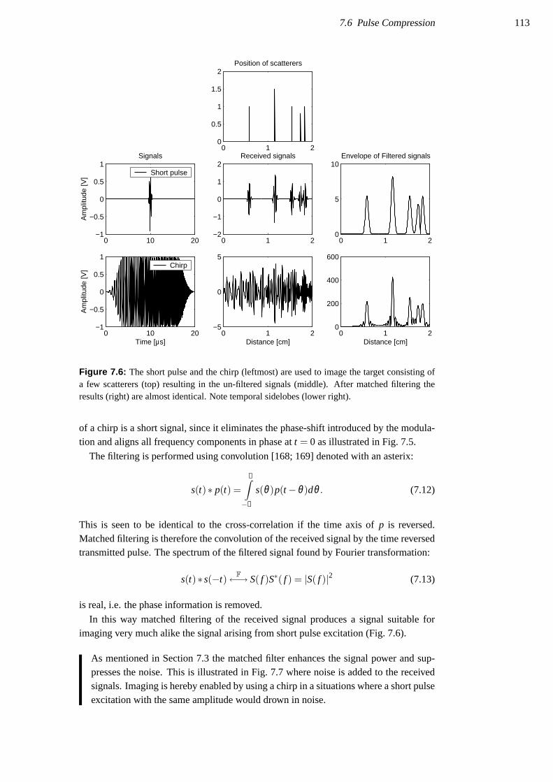
7.6 Pulse Compression 113

0 1 20

0.5

1

1.5

2Position of scatterers

0 10 20−1

−0.5

0

0.5

1

Am

plitu

de [V

]

Signals

Short pulse

0 1 2−2

−1

0

1

2Received signals

0 1 20

5

10Envelope of Filtered signals

0 10 20−1

−0.5

0

0.5

1

Time [µs]

Am

plitu

de [V

]

Chirp

0 1 2−5

0

5

Distance [cm]0 1 2

0

200

400

600

Distance [cm]

Figure 7.6: The short pulse and the chirp (leftmost) are used to image the target consisting ofa few scatterers (top) resulting in the un-filtered signals (middle). After matched filtering theresults (right) are almost identical. Note temporal sidelobes (lower right).

of a chirp is a short signal, since it eliminates the phase-shift introduced by the modula-tion and aligns all frequency components in phase at t = 0 as illustrated in Fig. 7.5.

The filtering is performed using convolution [168; 169] denoted with an asterix:

s(t)∗ p(t) =∞∫−∞

s(θ)p(t−θ)dθ . (7.12)

This is seen to be identical to the cross-correlation if the time axis of p is reversed.Matched filtering is therefore the convolution of the received signal by the time reversedtransmitted pulse. The spectrum of the filtered signal found by Fourier transformation:

s(t)∗ s(−t) F←→ S( f )S∗( f ) = |S( f )|2 (7.13)

is real, i.e. the phase information is removed.

In this way matched filtering of the received signal produces a signal suitable forimaging very much alike the signal arising from short pulse excitation (Fig. 7.6).

As mentioned in Section 7.3 the matched filter enhances the signal power and sup-presses the noise. This is illustrated in Fig. 7.7 where noise is added to the receivedsignals. Imaging is hereby enabled by using a chirp in a situations where a short pulseexcitation with the same amplitude would drown in noise.


0 10 20−1

−0.5

0

0.5

1

Am

plitu

de [V

]

Signals

Short pulse

0 1 2−5

0

5Received signals

0 1 20

2

4

6

8

10Envelope

0 10 20−1

−0.5

0

0.5

1

Time [µs]

Am

plitu

de [V

]

Chirp

0 1 2−5

0

5

Distance [cm]0 1 2

0

100

200

300

400

500

Distance [cm]

Compressed signal

Figure 7.7: Same signals and scatterers as shown in Fig. 7.6, but with noise added at a peak-signal-to-noise ratio equalling one. The resulting envelopes (right) clearly differ, since theshort pulse result (upper right) is mostly noise.

7.7 Temporal Sidelobes

One of the undesired side effects of the pulse compression mechanism is the introductionof temporal sidelobes (also called axial or range sidelobes) as shown in Fig. 7.6, whichare not present when short pulse excitation is used. This self-noise is a property of theauto-correlation function of the coded waveform and its effect on the image will be amasking of weak scatterers in the neighborhood of a strong scatterer.

In a previous work [170] a method has been proposed for the design of the coded FMwaveform and the compression filter that eliminates these axial sidelobes. This is doneby shaping the signal envelope as illustrated in Figures 7.2 and 7.6. The method is usedin the present study (see Methods), but the theoretical details are outside the scope ofthis paper, and the reader is referred to our previously published work [170; 171].

It should be noticed that the axial resolution does not depend on the chirp length, butequals 1/BW or slightly higher, matching conventional short pulse imaging [172].

The experienced sonographer knows very well about sidelobes in US images, espe-cially from older scanners and when scanning organs with a echo-poor backgroundsuch as the bladder. The sidelobes seen in conventional scanning, though, are lateralsidelobes that depend on the transducer aperture and the applied apodization (weight-ing of individual transducer elements). The lateral profile of an imaged point is theFourier transform of the apodized aperture (using the far-field approximation). Thetemporal sidelobes seen in the axial profile plot of an image of a point using chirp ex-citation and pulse compression are results of the convolution of the signal and filter.

7.8 Expected SNR Improvement 115

Lateral Distance [mm]

Pulsed Image

−40 −20 0 20 40

60

70

80

90

100

110

120

130

140

150−30 −20 −10 0

60

70

80

90

100

110

120

130

140

150

Dep

th [m

m]

Signal level[dB]

Central line

Lateral Distance [mm]

Coded Image

−40 −20 0 20 40

60

70

80

90

100

110

120

130

140

150−30 −20 −10 0

60

70

80

90

100

110

120

130

140

150

Dep

th [m

m]

Signal level[dB]

Central line

Figure 7.8: Images of wire phantom with 1 dB/(MHz ·cm) attenuation. Coded imaging (right)shows better penetration and less noise than conventional short pulse imaging (left).

7.8 Expected SNR Improvement

The improvement in SNR is theoretically equal to the time-bandwidth product of thetransmitted waveform. However, additional weighting is necessary in order to removeaxial sidelobes which will result in a loss of 1 to 2 dB [170; 171]. The ultrasoundtransducer and attenuation further reduce the expected SNR gain. For the FM signalused in this study (20 µs duration, centered at 4 MHz), the expected SNR gain will beon the order of 10 dB [173; 174]. Measurements from a wire phantom showed improvedsignal to noise ratio with improved visualization of deeply located wires (Fig. 7.8).

In liver tissue with an attenuation around 0.75 dB/MHz·cm (Table 1.2 on page 25) a10 dB improvement will result in an increased penetration of:

0.5 · 10 dB0.7dB/MHz·cm ·4 MHz

= 1.79 cm. (7.14)

117

Chapter 8

Material and Methods

If you don’t make mistakes,you aren’t really trying.

Coleman Hawking

Contents8.1 Equipment . . . . . . . . . . . . . . . . . . . . . . . . . . . . . . 1178.2 Pulses and Intensities . . . . . . . . . . . . . . . . . . . . . . . . 1188.3 Acquisition . . . . . . . . . . . . . . . . . . . . . . . . . . . . . . 1218.4 Data Processing . . . . . . . . . . . . . . . . . . . . . . . . . . . 1218.5 Automatic TGC Post-Correction . . . . . . . . . . . . . . . . . . 1228.6 Image Assessment . . . . . . . . . . . . . . . . . . . . . . . . . . 1248.7 Estimation of Penetration Depth . . . . . . . . . . . . . . . . . . 1248.8 Image Quality Comparison . . . . . . . . . . . . . . . . . . . . . 1258.9 Statistical Analysis . . . . . . . . . . . . . . . . . . . . . . . . . . 126

Nine healthy male volunteers were scanned in supine position by an experienced sono-grapher (MHP). Mean age was 32.6 (from 25.5 to 42.5) years, mean weight 76.9 (from65 to 93) kg and mean body mass index (BMI) was 23.5 (from 20.1 to 27.7).

8.1 Equipment

A modified clinical ultrasound scanner (Type 3535, B-K Medical A/S, Gentofte, Den-mark) was used with a mechanical transducer (Model 8534, 4 MHz pivoting focusedpiston type).

A single element focused transducer was used since we only had a single channelsystem with arbitrary pulse generation and digital sampling available at the time theexperiments were done.

The transmitter in the scanner was deactivated and an interface box attached to thetransducer connector allowed the use of an external transmitter. The low voltage signalsfrom the transmitter were amplified using a power RF amplifier (RITEC 5000) specifi-cally designed to drive ultrasound transducers.

Echoes were received, amplified, and time-gain compensated by the scanner and thensampled by an external receiver board (12 bits resolution, 40 MHz sampling rate). Trans-mitter and receiver boards were both developed and produced at CFU as a part of our Re-motely Accessible Software-configurable Multi-channel Ultrasound System (RASMUS)[175]. Transmitter and receiver board were synchronized with the scanner (Fig. 8.1).


Modified USScanner

(B-K 3535)

Receiverboard

Transmitterboard

Triggerbox

RF signal

Control PC

Interfacebox

RF PowerAmp

(Ritec 5000)

PCI Bus

PCI Bus

Signal

High Voltage Signal

Transmit and receivesignal

Receivedsignal

GPIB bus

EthernetTCP/IP

Frame & Line Trigger

Trigger

Display PC

Transducer

Figure 8.1: Schematic representation of experimental set-up. The scanner’s transmission circuitis by-passed and the received RF-signal is tapped after TGC amplification in the scanner.

With this configuration the live B-mode display on the scanner allowed orientation ofthe transducer before and during acquisition.

The transmitter’s ability to rapidly toggle between different pulse types during scan-ning was utilized to record pulsed and coded images interleaved. Hereby, every secondframe was pulsed and coded respectively, providing images of the exact same locationbeing directly comparable. The recording was done at 13 frames per second (fps), yield-ing 6.5 fps of each of the two kinds. The acquired data were stored as raw RF-data onhard-disk for off-line processing.

8.2 Pulses and Intensities

The short pulse used was a 2-cycle Hanning weighted cosine at 4 MHz with a 65 percentfractional bandwidth (-3 dB). The coded waveform was a linear FM signal sweeping afractional bandwidth of 110 percent. The signal was shaped using a Tukey window with

8.2 Pulses and Intensities 119

Figure 8.2: XYZ system forintensity measurements, show-ing the three axes for com-puter controlled movement of hy-drophone relative to the trans-ducer mounted in the water bath.

a duration of 0.15 times pulse duration [170], resulting in a transmitted signal with afractional BW of 65 percent like the short pulse.

The transducer was driven at approximately half the voltage used by the ultrasoundsystem manufacturer i.e. 70 V and 58 V peak-to-peak for short pulse and chirp respec-tively.

Intensity measurements were done using a computer controlled XYZ-system, wherethe transducer is mounted in a bath with degassed water. A calibrated hydrophone (aminute US transducer) were used to do the measurements. The hydrophone convertspressure (p) to voltage v:

v = pML( fc), (8.1)

by multiplication with the conversion factor ML( fc) which changes with frequency( fc). It is almost constant, though, within the frequency range examined in this work.Using this equation (8.1) the instantaneous intensity (i) can be found:

i = p2/ρc =v2

M2L( fc)ρc

, (8.2)

where ρ is the mass density of water (∼ 1000 kg/m3) and c the sound velocity(1480 m/s).

Intensity measurements to characterize an ultrasound system are performed in wa-ter. Measured intensities reported for approval before clinical use are so-called der-ated (in-vivo) values, which are lower than the actual measured (non-derated) inten-sities.

Derating is done to mimic the attenuation of sound in tissue. Therefore the mea-sured values are attenuated by of 0.3 dB/cm/MHz along the beam axis for equipmentapproval, which is on the safe side compared to the actual attenuation values of hu-man tissue (Table 1.2 on page 25. Derated parameters are usually denoted with asubscript ”.3”.

All intensity measurements for safety approval must be done at the location wherethe maximum derated pulse intensity integral (PII.3) is found [176]:

PII.3[J/cm2] = 10−0.3 dB/cm/MHz· fcz/10PII, (8.3)

where

PII[J/cm2] =

t2∫t1

v2h(t)dt

104[cm2/m2]ρcM2L( fc)

=t2∫

t1

i dt. (8.4)


Table 8.1: Intensity limits set by FDA. Based on numbers from [177] without permission. †:Other includes abdominal, intraoperative, pediatric, small organ (breast, thyroid, testes, etc.),neonatal cephalic, and adult cephalic. ‡: Either the ISPPA.3 or the MI limit must be met.

Use ISPTA.3 I‡SPPA.3 MI ‡

(mW/cm2) (W/cm2)

Peripheral Vessel 720 190 1.9Cardiac 430 190 1.9Fetal Imaging & Other † 94 190 1.9Ophthalmic 17 28 0.23

This is the integration of the intensity over the duration (T = t2− t1) of the pulse.The deration factor in (8.3) changes with depth (z). In practice the calculation can bedone by the oscilloscope recording the waveform from the hydrophone, so that theiterative search for maximum in the water tank is facilitated.

The measurements and limits required to get medical ultrasound equipment ap-proved in the United States are described in [177]. The intensity limits are not basedon any evidence but taken from a report of known intensity values in existing equip-ment in the 1970’ies where no adverse effects from ultrasound had been previouslyseen [178]1. The limits are listed in Table 8.1. Approval of equipment exceedingthose values requires further justification. If equipment is to be used for fetal Dopplerapplications there are further requirements, the so-called Output Display Standarddescribed in [177] as Track 3, which have to be met. This includes real-time displayof mechanical (MI) and thermal indices (TI) as described in [179]. Since this studysolely included male volunteers only Track 1 measurements were done.

The mechanical index is calculated from the derated peak rarefactional (∼ nega-tive) pressure value pr.3 in [MPa]:

pr.3 =∣∣∣∣ vn

M2L( fc)

∣∣∣∣10−0.3 dB/cm/MHz· fcz/20, (8.5)

measured at the location where the maximum PII.3 was found.

MI =pr.3

CMI√

fc, (8.6)

where CMI = 1MPa/√

MHz is merely a ’unit-removing’ constant.The spatial peak pulse average intensity (ISPPA) is easily found from the PII:

ISPPA,.3 = PII.3( j,v,zm, j,PII.3)/PD, (8.7)

where PD it the pulse duration.The spatial peak temporal average intensity (ISPTA is found by averaging the emit-

ted intensity over a recorded image frame consisting of several beam emissions (n) indifferent directions:

ISPTA.3 =n

∑i=0

PIIi ·SRF, (8.8)

where SRF is the scan repetition frequency (same as frame rate). The hydrophone isstationarily located in the center beam at the point where the PII.3 is maximum.

8.3 Acquisition 121

Table 8.2: Measured ultrasound intensities of the experimental set-up

Pulsed Coded

In waterIspt p 12 25 W/cm2

Isppa 3.0 1.8 W/cm2

Ispta 0.019 0.46 mW/cm2

In situIspt p 1.8 3.6 W/cm2

Isppa 0.43 0.26 W/cm2

Ispta 2.8 ·10−3 6.6 ·10−2 mW/cm2

MI 0.08 0.12

Table 8.3: Scanning locations. The third location was chosen to obtain largest possible scandepth in liver tissue.

No. Location

1 Sub-costal transverse section of right liver lobe.2 Sub-costal sagittal section of right liver lobe including right kidney.3 Epigastric transverse section of liver pointing to the right depicting the right liver lobe.

For both pulsed B-mode and coded excitation, intensity measurements were carriedout using a calibrated hydrophone in a water-tank with a computer controlled positioningsystem. Standard intensities and mechanical index were estimated (Table 8.2). As onecan see, the intensities are much lower than the recommended maximum values, withmechanical indices (MI) 0.08 and 0.12 for pulsed and coded imaging respectively. Thedifference between those values and the original scanners maximum MI=0.7 can, apartfrom the voltage difference, be explained by a sub-optimal impedance matching betweentransmit amplifier and the transducer interface.

8.3 Acquisition

Three different views were scanned in each person (Table 8.3). In this way three ac-quisitions, with the two different techniques were done in nine volunteers yielding 54cine-loop sequences (27 paired sequences).

The three locations (Fig. 8.3) were chosen to create US image sequences with eas-ily recognizable structures. Also, images of that region can almost always be madewithout artifacts from overlying air or other bowel content.

It was possible to switch between this interleaved acquisition mode and pure pulsedB-mode, to initially locate organs and position the transducer before acquisition. Ateach of the three locations, the volunteer was asked to hold his breath and an interleavedsequence of 2 seconds (30 frames) duration was recorded.

8.4 Data Processing

All data and image processing were carried out using MATLAB� (MathWorks Inc.,Natick, Mass., USA).


(a) Sub-costal transverse (b) Sub-costal sagittal (c) Sub-xiphoid transverse

Figure 8.3: The three locations used for image acquisition.

Both coded and pulsed data were compressed by the appropriate filter to maximizeSNR. The short pulse signal was compressed using a matched filter, the chirp was com-pressed using the mismatched filter described in [170], which is the linear FM signalweighted using a Chebyshev window with an 80 dB sidelobe level. Then envelope de-tection (Hilbert transform followed by absolute value) and log-compression were carriedout.

The TGC was corrected before scan-line conversion using automatic post-processingbased on statistical properties of the recorded data.

8.5 Automatic TGC Post-Correction

The time-gain-compensation amplifier in the scanner normally corrects the receivedsignal by increasing amplification over time as described in Section 1.2.1 on page 25.Since biological tissue usually does not attenuate equally everywhere this preset valuehave to be adjusted either manually by the sonographer during scanning based on theimages he sees on the monitor, or by some automatic TGC correction function inthe scanner. Since the images recorded in this trial are all created off-line severalhours after acquisition the first method is not an option, and therefore some manualor automatic post-processing method had to be developed to obtain images withouttoo aggravating TGC artifacts that were suitable for presentation to a clinical doctor.The experimental system used further complicated matters by consistently producinga ’skewed’ brightness distribution as illustrated in Fig. 8.4, where signals graduallydecreases 40 to 55 dB in amplitude from 0 to 10 cm even after the analog TGCcorrection performed by the scanner. As it can also be seen the fall-off is differentbetween pulsed and coded excitation. Therefore an automatic method was chosen,to provide an un-biased correction avoiding the investigator (MHP) to favorize one

8.5 Automatic TGC Post-Correction 123

0 5 10 15−20

0

20

40

60

Pulsed

Env

elop

e [d

B]

0 5 10 15

0

20

40

60

80

Coded

Env

elop

e [d

B]

0 5 10 15

−60

−40

−20

0Pulsed − TGC corrected

Depth [cm]

Env

elop

e [d

B]

0 5 10 15

−60

−40

−20

0Coded − TGC corrected

Depth [cm]

Env

elop

e [d

B]

Figure 8.4: Maximum, me-dian, and minimum curvesbefore (top row) and af-ter (bottom row) TGC post-processing. The spline andthe levels used for approxi-mation can be seen on the up-per plots.

from the other before presentation to the clinical evaluators. Also the method had toresult in ’similar looking’ images. That would be that pulsed and coded images of thesame structure should have more or less same brightness in corresponding parts ofthe images, but also allow one to be brighter of darker in the same part if significantdifferences due to the different acquisition method should give rise to that. A taskwhich at first glimpse seems impossible.

An ordinary up- and down-regulation of amplitude according to mean or max val-ues have been used earlier at the center, without great results. Both are very sensitiveto hyper-echoic structures that stand out and do not represent the overall image verywell. So a method that could take both the signal representing the imaged structures,the inherent noise, and could ignore irrelevant peak-values were sought.

To obtain uniform images with identical brightness and contrast at all depths in bothconventional and coded imaging an automatic TGC post-processing was applied to allimages (cine-loops).

From the first frame of each sequence the median value of all 105 lines in an imageat each depth was calculated. The values used for this calculation were the logarithmicenvelope:

envlog(t) = 20 · log10 |s(t)+ j · s(t)| , (8.9)

where s(t) is the Hilbert transform [180] of s(t). This median curve was fitted by acubic spline using 8 control points calculated from the mean of the curve in the regionsurrounding the control points with the same size as the control point inter-distance(Fig. 8.4).

The resulting spline was subtracted from every line in all images in the correspondingcine-loop, resulting in images with a median value around 0 dB. By subtracting 30 dBand displaying dynamic range of 40 dB (from -40 to 0 dB) signals higher than 30 dBabove the median and lower than 10 dB under the median were cut off.

The method was empirically derived with the knowledge of the median filter’s ro-bustness to extreme values in mind. Since noise is present everywhere in the images,minimum values must represent nothing but noise, maximum values extreme signal


Figure 8.5: Layout of cine-loop presentation of single images. Left and right images are identi-cal except for the overlayed rulers on the right used to determine the depth estimated by lookingat the left image

amplitudes also including noise, whereas the median could be assumed to be a goodrepresentative for the image signal level.

Initial evaluation on several image acquisitions showed a very robust correctionproviding very smooth and homogeneous image results with the ’right look’ as the onean experienced sonographer tries to obtain by manually adjusting the depth dependentTGC sliders on the scanner. Furthermore, pulsed and coded images looked fully alikewith regards to TGC settings. The approach has at the time of writing only beensubjectively evaluated. A blinded comparison of the resulting image quality to thequality of images obtained using conventional TGC adjustments by an experiencedsonographer remains yet to be carried out.

8.6 Image Assessment

Every image sequence was converted to movie clips (AVI-files using loss-less compres-sion2) for evaluation on an ordinary PC. Three experienced sonographers (medical doc-tors) evaluated the cine-loops. None of the three were involved in the project, nor hadthey any prior knowledge about the details of coded imaging or seen any of the imagesbeforehand. Evaluations were done blinded and independently of each other.

8.7 Estimation of Penetration Depth

All 54 sequences, either pulsed or coded, were presented in random order to each sono-grapher with no information on the type of technique used.

For each sequence the sonographer answered two questions:

2Huffyuv CODEC v2.1.1, http://web.archive.org/web/*/www.math.berkeley.edu/ benrg/huffyuv.html

8.8 Image Quality Comparison 125

- Question 1: At what depth [cm] does the image quality decrease significantly?

- Question 2: At what depth [cm] does the image quality become insufficient forclinical diagnosis?

The movies were presented using a two-part view, with a left part for image assess-ment and a right part for finding the actual depth using overlayed rulers (Fig. 8.5).

Every sonographer undoubtedly has his own perception of image quality resulting in anot negligible inter-observer variation in the absolute depth estimation. This is compen-sated for by examining the differences between depths within the pairs of conventionaland coded images. Moreover, some of the variation between different persons scannedand between locations is removed that way.

8.8 Image Quality Comparison

To compare the image quality of coded and conventional imaging, matching pairs ofimage sequences recorded at the exact same location were showed simultaneously side-by-side in random order.

The pairs were shown with the coded image placed to the left or the right randomlyto avoid bias from potential left-right preferences or expectancies in the examiners, andpossible influences from the surroundings (e.g. lights). To test whether such influenceexisted, examiners saw both orientations during the evaluation.

For each of the 27 image pairs, two cine-loops were created. The images were croppedbelow the depths: dmagiq and dmaui calculated for each image pair from the answers toQuestions 1 and 2:

dmagiq = min

N∑

n=1dn,Q1,C

N,

N∑

n=1dn,Q1,P

N

(8.10)

dmaui = max

N∑

n=1dn,Q2,C

N,

N∑

n=1dn,Q2,P

N

(8.11)

where N is the total number of examiners and d1,Q2,C means examiner one’s answer toQuestion 2 for the coded image.

The first depth (dmagiq) represents the “minimum average good image quality” depthfor the image pair. The second (dmaui) represents the “maximum average usable image”depth.

Comparison of the images cropped at dmagiq therefore only evaluates image qualitywithin a range, where both techniques should provide good image quality according tothe sonographers’ first evaluation (Section 8.7).

The comparison of image pairs cut at dmaui evaluates image quality within the maxi-mum usable range of that pair judged by the sonographers. In this case, images producedby the technique with best penetration are expected to do best.

The reason for this distinction was to evaluate, not only if codes could improve imagequality by increasing penetration depth (dmaui), but also whether it can provide the sameimage quality at the range readily obtainable by conventional pulsed ultrasound imaging(dmagiq).


Figure 8.6: Presentation of image pair cine-loops. In this case the left is done using codes andright is a conventional image.

Equally goodLeft is

uselessRight isuseless

BetterMuchbetter

BetterMuchbetter

0 10 20 30 40 50 60 70 80 90 100 110 120

Left better Right better

Figure 8.7: Explanation of VAS shown to sonographers before scoring images. The lower scalewas used to read scored values.

At presentation of the 54 pairs, in random order and with random left-right placing ofthe two kinds of images, the sonographers were asked which of the two images was better(Fig. 8.6) by scoring on a visual analog scale (Fig. 8.8). Before doing the evaluation thesonographers were showed the explanation of the VAS depicted in Fig. 8.7 to ensure aproper use of the scale’s range. To avoid attraction to the divisions of the scale shown inFig. 8.7, the explanation was not allowed near the scoring scales during evaluation.

8.9 Statistical Analysis

The statistical data analysis language R (http://cran.r-project.org/) was used for statisticalcomputations.

Depth Comparisons Student’s (one sample) t-test was used on the resulting differ-ences in penetration depth, assuming normal distribution supported by Fig. 9.2. Two-sided tests were used.

8.9 Statistical Analysis 127

Figure 8.8: Visual Analog Scale (VAS) used to compare left and right image.

Image Quality Comparisons Since each sonographer most likely has his own in-terpretation of the visual analog scale and show different degrees of attraction to thecenter point (Fig. 9.3), no assumptions of normal distributed data were made. Conse-quently, Wilcoxon signed rank test with continuity correction was used on VAS results.

129

Chapter 9

Results

It is an old maxim of minethat when you have excluded the impossible,whatever remains, however improbable,must be the truth.

Sir Arthur Conan Doyle - The Beryl Coronet

Contents9.1 Limitations and Artifacts . . . . . . . . . . . . . . . . . . . . . . 1299.2 Penetration . . . . . . . . . . . . . . . . . . . . . . . . . . . . . . 1309.3 Image Quality . . . . . . . . . . . . . . . . . . . . . . . . . . . . 130

The resulting coded ultrasound images were generally good, with less noise and betterpenetration than corresponding conventional images. Otherwise, the two kinds of imageslooked alike with no apparent differences.

9.1 Limitations and Artifacts

The spatial length of the coded waveforms around 3 cm means that image formationcannot be suspected to be fully developed closer to the transducer than half this lengthi.e. 1.5 cm, nor deeper than 1.5 cm from the depth where line sampling stops.

When very strong reflectors (e.g. the diaphragm or vessel walls) occurred in the im-ages a kind of repeating echoes were seen (Fig. 9.1) when using coded excitation. Theimages made using conventional excitation did not show this artifact.

[cm]

[cm

]

Pulsed

0 1 2 3 4 5

10

11

12

13

14

15

[cm]

[cm

]

Coded

0 1 2 3 4 5

10

11

12

13

14

15

Figure 9.1: Artifact at di-aphragm seen in coded imageonly. Notice one big artifact be-fore the diaphragm and severalafter.


Question 1

Difference [cm]

Fre

quen

cy−2 0 2 4 6 8

010

2030

Question 2

Difference [cm]

Fre

quen

cy

−2 0 2 4 6 8

010

2030

−2 0 1 2

−2

02

46

Normal Q−Q Plot


Sam

ple

Qua

ntile

s

−2 0 1 2−

20

24

Normal Q−Q Plot


Sam

ple

Qua

ntile

s

Figure 9.2: Histograms and normality plots of depth differences (dcoded−dpulsed) from answersto questions 1 and 2, supporting the assumption of normally distributed data.

Examination of the corresponding RF-lines revealed saturation of the scanner TGC-amplifier explaining the artifacts. Harmonics produced by the amplifier will result intranslation of energy along the time axis, when the filter is applied to the signal. Higherharmonics will therefore appear closer to the transducer.

Temporal sidelobes below -50dB [170; 171] could also explain the artifact at the di-aphragm. The limited SNR in the experimental system precluded us from evaluating thatfurther.

9.2 Penetration

Figure 9.2 shows the distributions of differences between coded and conventional imag-ing. The results are listed in Tables 9.1 and 9.2. All three examiners found highlysignificant improvements in imaging depths answering both questions 1 and 2. The av-erage increase in penetration depth was 1.98 cm [examiner range 0.7–3 cm] in question1 and 1.85 cm [examiner range 1.2–2.2 cm] in question 2.

9.3 Image Quality

The results from image quality comparisons are depicted in Fig. 9.3.

In cine-loops cropped at dmagiq the difference between conventional and coded imag-ing was just barely there, though significantly in favor of coded imaging, with examiner

9.3 Image Quality 131

Question 1

Examiner Pulsed Coded Diff. Conf. int. P[cm] [cm] [cm] 95% value

S1 5.63 8.65 3.02 2.00 –4.04 <0.001S2 8.85 9.59 0.741 0.308–1.17 <0.005S3 8.80 11.0 2.17 1.65 –2.69 <0.001

Pooled 7.76 9.73 1.98 1.53 –2.42 <0.001

Table 9.1: Results of answers to Question 1:“At what depth [cm] does the image quality de-crease significantly?”

Question 2

Examiner Pulsed Coded Diff. Conf. int. P[cm] [cm] [cm] 95% value

S1 8.91 11.1 2.24 1.60 –2.88 <0.001S2 11.6 12.8 1.19 0.564–1.81 <0.001S3 10.4 12.6 2.13 1.65 –2.61 <0.001

Pooled 10.3 12.2 1.85 1.51 –2.19 <0.001

Table 9.2: Results of answers to Question 2:“At what depth [cm] does the image quality be-come insufficient for clinical diagnosis?”

S1 − d magiq

VAS score

Fre

quen

cy

−60 −20 20 60

020

40

S2 − d magiq

VAS score

Fre

quen

cy

−60 −20 20 60

020

40

S3 − d magiq

VAS score

Fre

quen

cy

−60 −20 20 60

020

40

S1 − d maui

VAS score

Fre

quen

cy

−60 −20 20 60

020

40

S2 − d maui

VAS score

Fre

quen

cy

−60 −20 20 60

020

40

S3 − d maui

VAS score

Fre

quen

cy

−60 −20 20 60

020

40

Figure 9.3: Distribution of answers to imagecomparisons of images cut at dmagiq (left) anddmaui (right) respectively. Data are shown for thethree sonographers (S1-S3) individually.


Table 9.3: Mean VAS differences foreach examiner evaluating images cut atdMAUI and dMAGIQ. Positive value meanscoded image is better.

Sonographer DifferencedMAGIQ dMAUI

S1 3.31∗∗ 18.5∗∗∗

S2 1.61∗ 13.9∗∗∗

S3 1.72† 5.87∗∗

***: P<0.001 , **: P<0.005, *: P<0.05, †: P=0.05

mean values from 1.61 to 3.48 on the VAS ranging from -60.0 to 60.0 (Table 9.3).The difference was more pronounced in images cropped at dmaui with mean scores

18.5, 13.9, and 5.87 respectively; highly significant in favor of coded imaging (Ta-ble 9.3).

A small, but significant left/right positioning bias was found in one case (sonographer2 at dmagiq). Such a difference results in a mean VAS score closer to zero, i.e. anunderestimation of the difference between pulsed and coded imaging.

133

Chapter 10

Discussion

Anyone who conducts an argumentby appealing to authorityis not using his intelligence;he is just using his memory.

Leonardo Da Vinci

The experimental setup allowing simultaneous recording of both coded and conventionalpulsed excitation images, provided a good platform for a direct comparison of pairedimage sequences acquired under the exact same circumstances.

This approach enabled by the RASMUS system is continuously used at our laboratoryso that every new technique can be directly compared to conventional technique un-der exact same circumstances even when imaging in-vivo. This provides immediateobjective feedback which is invaluable in the development cycle.

To our best knowledge clinical evaluation of coded excitation has not been reportedbefore (PubMed - Medline). The present work shows that coded excitation performswell in-vivo. No severe artifacts except repeating echoes before and after very strongspecular reflectors, such as the diaphragm, were encountered. We believe this problemwill be solved using optimized receive amplifiers.

The estimated gain in penetration depth around 2 cm using coded excitation is smallerthan the expected 3.2 cm derived from a 10 dB SNR improvement at 4.5 MHz witha 0.7 dB/(cm ·MHz) attenuation. One cause could be the fact that full penetrationthroughout the liver was almost possible when scanning the relatively slim volunteersat 4.5 MHz, even at the very low intensities used. If conventional imaging penetrates tothe diaphragm, no improvement in penetration using codes will be detected. This pointcan be tested repeating the experiment at higher frequencies.

Actually, as stated in the methods section, the experiments were done at a centerfrequency of 4.0 MHz. The resulting improvement in penetration depth is therefore:

0.510 dB

4 MHz ·0.7 dB ·cm−1 ·MHz−1 = 1.79 cm. (10.1)

This is actually close to the values found by the clinical evaluation, although a bitsmaller. The value lies within the confidence intervals for the pooled data (Tables 9.1and 9.2 on page 131). Therefore the experimental results actually agreed better withthe predicted than stated in the published paper.


The intensities used in this work (Table 8.2) were all much lower than intensitiesnormally used in medical ultrasound [181]. The mere difference of waveforms partlyexplains that the chirp has higher Ispt p and lower Isppa than the short pulse excitation.Additionally, the fact that the transmit amplifier was driven at the edge of its abilities,might play a role.

Around the first one and a half centimeter will be missing in the image, when usingcodes of three centimeters length. This will rarely be of any importance in abdominalscanning, especially not in cases where increased penetration is desired. Otherwise,conventional imaging can be used for the superficial imaging. The missing part at thedeep end can be compensated for by increasing sampling time per line accordingly. Thiswill result in a 10% decrease of frame-rate, when scanning at 15 cm depth

As predicted by previous simulations and in-vitro studies, coded excitation increasedthe SNR resulting in higher penetration depths in a clinical setting too. Blinded eval-uation by sonographers (medical doctors) demonstrates a highly significant increase ofpenetration depth. Furthermore, they significantly preferred images done using codedexcitation - even when cut off below penetration depths of conventional images.

The hypotheses listed in Section 7.1 on page 108, were both rejected.

The clinical benefit of increased penetration is obvious to the sonographer that dailyexperiences cases with insufficient penetration resulting in diagnostic uncertainty. Alter-natively, a frequency increase yielding higher resolution whilst maintaining penetrationis also appealing. The possible improvement of diagnosis, treatment and prognosis,though, remains to be tested in randomized controlled trials.

The safety limits on medical ultrasound may certainly limit the use of coded excitationin conventional systems, whereas real-time 3D and synthetic transmit aperture (STA)systems most likely will benefit from using coded excitation [182; 183]. The sphericalwavefronts used in STA imaging, created by only a few transducer elements, yield lowpeak intensities – especially when using 2D transducer arrays for real-time 3D imaging,due to their very small elements.

135

Part IV

Conclusion

137

Chapter 11

Overall Discussion and Perspectives

If we had had more time for discussionwe should probably have made a great

many more mistakes.

Leon Trotsky

Contents11.1 3D Ultrasound Scanning of Cervix Cancer . . . . . . . . . . . . 13711.2 Coded Excitation . . . . . . . . . . . . . . . . . . . . . . . . . . . 13811.3 Perspectives . . . . . . . . . . . . . . . . . . . . . . . . . . . . . 139

The results and immediate implications of the two trials have been discussed in Chap-ters 6 and 10. In the following a more general discussion and outline of future perspec-tives will be attempted.

11.1 3D Ultrasound Scanning of Cervix Cancer

If, or rather when, the three-dimensional ultrasound scanning technique will be able todeliver high quality images covering covering most of the pelvis, and to do it consis-tently for every patient, it will undoubtedly become an important diagnostic tool in thetreatment of cervix cancer. Ultrasound scanning is not only fast, painless, and safe, butalso relatively inexpensive, which makes it a realistic option also parts of the world lessprivileged than ours.

The importance of ultrasound scanning in almost every medical speciality of medicine,especially within surgery for pre-operative assessment, indicates that it could also playan important role in pre-operative evaluation of cervical cancer.

Only one work [148] evaluating 3D ultrasound scanning of cervical cancer has beenpublish until now. It compared tumor volume estimation using two- and three-dimen-sional US to volumes estimated by histology (IB and IIA cancers only). The otherpublished work about cervical 3DUS concerns morphologic description of the cervixduring pregnancy in a population of women at high risk of preterm delivery [95]. So thestaging approach using 3DUS is new, and the relatively good results yielded by usingsub-optimal equipment in the hands of a non-gynecologist indicate a potential future forthe technique.

Magnetic resonance imaging has just like computerized tomography been used in theevaluation of cervical cancer, both in routine clinical settings and research - especiallybefore and after radio- and chemotherapy. It has also been evaluated as a staging toolon several occasions [115–124]. No clear evidence for major benefits exists, but it must

138 Chapter 11 Overall Discussion and Perspectives

also be emphasized that the single modality imaging technique is usually compared to astaging routine carried out by a team of experienced clinical doctors using several toolsto perform the FIGO staging procedure. In that light, the MRI staging results are not atall bad, and was therefore chosen as a means of verifying the 3DUS and clinical findingsin the present trial. Especially since no other method could provide that informationabout patients not operated upon, as safely as MRI could.

If the planned number of patients had been achieved with both 3DUS and three-dimensional MRI acquisitions, obviously, a more solid foundation for clear conclusionswould exist. Especially because a three-dimensional description of the region wouldhave been produced by two different modalities. This could potentially provide new in-formation in the 60 percent of the cases, in which the FIGO staging result is usually thefinal statement.

Whether 3DUS should be done using transrectal or transvaginal transducers - or acombination - is not possible to decide, from the currently existing knowledge. Thiswill eventually be a decision based on several factors such as imaging quality, technicalpossibilities, patient compliance, and (not the least) marketing decisions.

The three-dimensional imaging technique might also be useful for planning and mon-itoring radiation- and adjuvant chemo-therapy, just as conventional ultrasound and CTare used for that purpose today.

As every diagnostic method has its weak and strong points, the field of multi-modalityimaging, where information from two or more modalities are merged, is an obvious wayto pursue. Three-dimensional data sets of the same regions can be aligned and presentedas one using such techniques. This was primitively done in the present works, by manualalignment of ultrasound, MRI, and histology volumes in the same visualization softwareto make the direct comparisons. A method combining the large field-of-view of MRIinto one image (volume) with ultrasound, that provides local high resolution images,could be a way to achieve large enough volumes with satisfying resolution to cover bothsmall and large tumors.

Other aspects are in favor of three-dimensional imaging. The acquisition and stor-age of a whole volume makes the examination better documented than any other typeof examination. It offers the ability to do a second evaluation, if desired by an expertat another hospital, where the examiner has more possibilities to manipulate and selectslices than with conventional two-dimensional images. Also a comparison of acquisi-tions made at different times can be done more accurately, since the exact same viewscan be reconstructed for direct comparisons.

11.2 Coded Excitation

The coded excitation approach using chirp signals has proven to be so advantageous androbust that it is used continuously in our lab when developing other new techniques. Itis possible - in fact advantageous - to use it together with other advanced imaging tech-niques such as synthetic aperture imaging [182; 183], vectorial flow techniques [184],real-time 3DUS [185], and harmonic contrast imaging [186].

High end commercial products increasingly incorporate some sort of signal encodingor modulation to increase SNR, for instance the flow visualization technique called B-Flow (GE Medical) is based on coded excitation. It is only a matter of time before

11.3 Perspectives 139

integrated electronics become powerful and inexpensive enough, and we will see suchtechnology in most clinical scanners.

The clinical benefits of increased penetration and higher resolution in medical diag-nosis is obvious and will not be discussed further. The use of coded excitation doesincrease the average power transmitted closing in on the safety limits, which of courseshould be dealt with seriously. But for now, intensities are comparable to those of con-ventional Doppler, if used in a clinical setting. The intensities used in the present trialwere much lower than the limits set by the Food and Drug Administration the UnitedStates.

The ability to generate images using different techniques simultaneously on the samescanner, which done in the present trial, provides a robust way to compare conventionaland new techniques in-vivo. In most other medical research this is not possible and onehas to resort to randomized studies to achieve comparable groups that receives differenttreatments. This benefit will undoubtedly play an important role in future developmentand evaluation of imaging techniques.

11.3 Perspectives

At present we experience major new developments in medical ultrasound scanning pri-marily thanks to the rapid development in electronics and computers. As we have seengreat advances from A-mode and static B-mode, to dynamic B-mode and static 3D imag-ing, the next major technological shift to real-time 3D (4D) is lurking around the corner.

Real-time three-dimensional imaging may also be applied to cervical scanning. Al-though movement is not really a problem, it could provide better information of mobilityand fixation of the cervix to neighboring structures. It could also offer faster formationof volumes with a larger field-of-view, directionally compounding, and higher resolutionwhilst simultaneously decreasing the acquisition time.

In all fields of medical ultrasound scanning, real-time 3D will undoubtedly bring ma-jor advances - not only to diagnostic but especially to interventional ultrasound. Muchmore effective tracking of instruments - multiple simultaneously - during procedures willenable a whole new range of minimally invasive treatments.

140 Chapter 11 Overall Discussion and Perspectives

141

Part V

Appendices and Bibliography

143

Appendix A

FIGO Stages

Below are the stages as defined by the International Federation of Gynecology and Ob-stetrics (FIGO) - see Benedet et al. [187]. The grayed rows are not used for staging, butare either super-groups or in the case of stage IIIC a pathological extension. sub-divisionof the stage.

Stage Definition TNM Treatment

0 Carcinoma in situ, cervical intraepithelialneoplasia Grade III.

Tis N0 M0 Conisation

I The carcinoma is strictly confined to thecervix (extension to the corpus would bedisregarded).

IA Invasive carcinoma which can bediagnosed only by microscopy. Allmacroscopically visible lesions — evenwith superficial invasion — are allotted toStage Ib carcinomas. Invasion is limited toa measured stromal invasion with amaximal depth of 5.0 mm and a horizontalextension of not > 7.0 mm. Depth ofinvasion should not be > 5.0 mm takenfrom the base of the epithelium of theoriginal tissue — superficial or glandular.The involvement of vascular spaces —venous or lymphatic — should not changethe stage allotment.

IA1 Measured stromal invasion of not> 3.0 mm in depth and extension of not> 7.0 mm.

T1a1 N0 M0 Conisation – 5yrsfollow-up

IA2 Measured stromal invasion of > 3.0 mmand not > 5.0 mm with an extension of not> 7.0 mm.

T1a2 N0 M0 Simple totalhysterektomy

IB Clinically visible lesions limited to thecervix uteri or preclinical cancers greaterthan Stage Ia.

T1b N0 M0 Radical hysterektomy

IB1 Clinically visible lesions not > 4.0 cm. T1b1 N0 M0IB2 Clinically visible lesions > 4.0 cm. T1b2 N0 M0IC T1c N0 M0II Cervical carcinoma invades beyond the

uterus, but not to the pelvic wall or to thelower third of the vagina.

IIA No obvious parametrial involvement. T2a N0 M0 Radical hysterektomyIIB Obvious parametrial involvement. T2b N0 M0 Onchologic treatment.

Intracavitary andexternal radiotherapycombined withchemotherapy.

144 Appendix A FIGO Stages

III The carcinoma has extended to the pelvicwall. On rectal examination, there is nocancer-free space between the tumour andthe pelvic wall. The tumour involves thelowerthird of the vagina. All cases withhydronephrosis or non-functioning kidneyare included, unless they are known to bedue to other causes.

IIIA Tumour involves lower-third of the vagina,with no extension to the pelvic wall.

T3a N0 M0 Onchologic treatment.

IIIB Extension to the pelvic wall and/orhydronephrosis or non-functioning kidney.

T3b N0 M0 Onchologic treatment.

IIIC T1 N1 M0T2 N1 M0T3a N1 M0T3b N1 M0

IV The carcinoma has extended beyond thetrue pelvis, or has involved(biopsy-proven) he mucosa of the bladderor rectum. A bullous oedema, as such, doesnot permit a case to be allotted to Stage IV.

IVA Spread of the growth to adjacent organs. T4 all M0 Onchologic treatment.IVB Spread to distant organs. all all M1 Onchologic treatment.

145

Appendix B

The Cohen Kappa Value

The Cohen kappa (κ) value is a measure-ment of agreement that takes the expectedagreement by chance into account.

If two observers A and B diagnoseswhether a condition is true or not, we couldget a result like in Table B.1.

Table B.1: Example results from two ob-servers A and B.

AYes No

B Yes 14 6 20No 4 11 15Total 18 17 35

The calculated observed agreement is

po =14+11

35= 0.714 (B.1)

From the row and column totals we cancalculate (Table B.2) the expected confu-sion matrix (Table B.3).

Table B.2: Calculation of expected values bychance

AYes No

B Yes 18·2035

17·2035 20

No 18·1535

17·1535 15

Total 18 17 35

Table B.3: Expected values - result

AYes No

B Yes 10.3 9.7 20No 7.7 7.3 15Total 18 17 35

From this the expected agreement bychance can be calculated:

pe =10.3+7.3

35= 0.502 (B.2)

The κ value is then calculated:

κ =po− pe

1− pe(B.3)

=0.714−0.502

1−0.502(B.4)

= 0.426 (B.5)

The guidelines in Table B.4 can be used tointerpret the κ-value.

Table B.4: Interpretation guidelines to κ val-ues (adapted from Altman [155]).

κ value Strenght of agreement

< 0.20 Poor0.21-0.40 Fair0.41-0.60 Moderate0.61-0.80 Good0.81-1.00 Very good

A 95% confidence interval can be calcu-lated:

κ±1.96se(κ) (B.6)

where the standard error is:

se(κ) =

√po(1− po)n(1− pe)2 (B.7)

The method is used in the same way on n-by-n tables.

146 Appendix B The Cohen Kappa Value

147

Appendix C

Software Documentation

ContentsC.1 Image Registration Tool . . . . . . . . . . . . . . . . . . . . . . . 148C.2 3D Data Conversion . . . . . . . . . . . . . . . . . . . . . . . . . 149C.3 Raw Binary Data Format . . . . . . . . . . . . . . . . . . . . . . 149C.4 Signal Processing and Movie Creation . . . . . . . . . . . . . . . 152

Several thousand lines of code has been written to do the data processing in thisproject. Therefore only a very short description of the different utilities is given in thisappendix.

148 Appendix C Software Documentation

Figure C.1: Marked lineROI selected before runningthe macro (left) and the re-sult (right).

C.1 Image Registration Tool

The small NIH Image macro shown in Listing C.1 translates and rotates the image toand around the center based on the line ROI selected (Fig. C.1). The macro languagemore or less follows Pascal syntax.

Listing C.1: Macro to rotate and translate slices to center.

1 { Alignment macro for Scion / NIH Image }

2 { Author: Morten H Pedersen, [email protected]}

3 { Select line ROI before calling by pressing ’X’ }

4 macro ’Center and Rotate [X]’ var

5 x1,y1,x2,y2: integer

6 width,height: integer

7 dx,dy: integer

8 x,y: integer

9 begin

10 {Get line ROI and calculate center and slope}

11 GetLine(x1,y1,x2,y2,width);

12 x := (x2+x1)/2;

13 y := (y2+y1)/2;

14 GetPicSize(width,height);

15 dx := x-width/2;

16 dy := y-height/2;

17 {Center}

18 MakeRoi((abs(dx)+dx)/2,(abs(dy)+dy)/2,width-abs(dx)-1,height-abs(dy)

-1);

19 Copy;

20 MoveRoi(-dx,-dy);

21 Paste;

22 {Clear Outside ROI}

23 Copy;

24 SelectAll;

25 Clear;

26 RestoreRoi;

27 Paste;

28 KillRoi;

29 {Rotate}

30 SetScaling(’Bilinear’);

31 SetScaling(’Same Window’);

32 SelectAll;

33 ScaleAndRotate(1,1,-180/3.14159265*arctan((y1-y2)/(x1-x2)));

34 end;

C.2 3D Data Conversion 149

Figure C.2: Hierarchyof C++ classes in thedizVolKonvertor software.

C.2 3D Data Conversion

A data conversion tool was developed to convert volume between proprietary formats.A simple class library was written in C++ for reading, writing, and manipulating volumedata. The class hierarchy depicted in Fig. C.2 consists of two main groups, namelysubclasses of the dizVol class that represent the volume data in memory, and subclassesof dizVolFile class providing file read and write functions. Not all classes are fullyimplemented at the moment. The classes can represent both 3 and 4 dimensional datasets.

For this thesis the file readers dizVolFileRawbin, dizVolFileAnalyze, dizVolFileLis,and dizVolFileKretz were used to convert dizVolCylinder and dizVolCartesian datasetsto the Kretz format.

A graphical user interface for conversion solely to the Kretz file format was made(using Microsoft Visual C++ v6.0). This gives access to free visualization of 3D and4D data sets in the free demo version of 3D View 2000. Data from other systems can beconverted using the raw binary data reading function, which is done with the histologicaldata slices in this thesis. The user interface of the conversion program is depicted inFig. C.3.

The program displays volume type, resolution, and data size before conversion. Linearinterpolation of all three spatial directions can be done if desired and resulting data sizeis calculated before conversion.

C.3 Raw Binary Data Format

As mentioned, the conversion tool can read raw binary stacks, like the ones produced byNIH Image or ImageJ. Data must consist of a single binary file with the .bin extension


Figure C.3: Program developed to convert 3D volume files to Kretz format (patient ID ismasked by black ’spray’).

and a format description text file (.txt-file) must be located in the same directory withthe same name. The description file must look like the example in Listing C.2.

Listing C.2: Raw data volume description file format.

1 % Volume description

2 % volume type: cartesian

3 type cartesian

4 bits 8

5 bigendian 0

6 max 255

7 min 0

8 inverse 0

9 % width [pixels]

10 % height [pixels]

11 % slices [pixels]

12 width 400

13 height 400

14 slices 50

15 volumes 1

16 % width pixel size [m]

17 % height pixel size [m]

18 % slices pixel size [m]

19 pixelwidth 0.0002

20 pixelheight 0.0002

21 slicedist 0.001

22 volumedist 1

Currently only reading of cartesian data-sets is implemented (C.2 line 3). Data mustbe ordered from left to right (x value), anterior to posterior (y value), and superior toinferior (z value ∼ slice no.). A volume with the left-right width (number of pixels)

C.3 Raw Binary Data Format 151

of Xwidth, anterior-posterior height Yheight , and superior-inferior depth Zslices (number ofslices) should have data ordered according to the index:

index = x+ y ·Xwidth + z ·Xwidth ·Yheight , (C.1)

where x∈ [0;Xwidth−1], y∈ [0;Yheight−1], and z∈ [0;Zdepth−1] to enable the orientationdepicted in Fig. 1.16(b) on page 36. If as binary stack is saved from NIH image the firstslice must be superior, left side in image must be patient left side, and upper part ofeach slice anterior. The reason for this convention is the format of the pathological slicesobtained in the project.


Figure C.4: TGC Correction Example. The upper two graphs are pulsed (left) and coded (right)before correction. The middle curves are after correction. The resulting images after correctionare shown below.

C.4 Signal Processing and Movie Creation

Several MATLAB scripts were use to create the movies used for evaluation of codedexcitation.

After initial preparation of the raw RF-data in one file per frame, compression, fol-lowed by envelope detection and temporal sub-sampling (from a sampling frequency of40 MHz to 20 MHz), log compression, scaling and conversion to 32 bit integers.

Then automatic TGC post-correction were done as described in Section 8.5 on page 122.An example of the image intensity curves is shown in Fig. C.4.

Scripts were made to perform the data processing as a batch of several hundred tasksthat were automatically run in parallel on a cluster consisting of 18 Linux and WindowsPCs.

Finally, the corrected image data was scan converted and made into movie files (Win-dows AVI format) compressed with a lossless Huffyuv CoDec1.

1Huffyuv CODEC v2.1.1, http://www.math.berkeley.edu/˜benrg/huffyuv.html

153

Appendix D

Publications

ContentsD.1 Review Paper: 3DUS in Obstetrics & Gynecology . . . . . . . . 153D.2 Case Report: 3DUS of Monoamniotic Twins . . . . . . . . . . . 163D.3 Paper: Chirp Coded Excitation in US . . . . . . . . . . . . . . . 167D.4 Related Publications . . . . . . . . . . . . . . . . . . . . . . . . . 180D.5 Presentations . . . . . . . . . . . . . . . . . . . . . . . . . . . . . 180

D.1 Review Paper: 3DUS in Obstetrics & Gynecology

M. H. Pedersen and T. Larsen. [three-dimensional ultrasonography in obstetrics and gy-necology]. Ugeskr. Laeger, 163(5):594–599, 2001a

This paper gives a review on the use of 3D US in Obstetrics and Gynecology. Thelist of references has been truncated by the journal publisher, but the remaining ones arelisted after the paper (see page 161).

154 Appendix D Publications

D.1 Review Paper: 3DUS in Obstetrics & Gynecology 155

594 V I D E N S K A B O G P R A K S I S

UG

ESK

R L

ÆG

ER 1

63/5

29.J

AN

UA

R 2

001

UL-scanning (US) er gennem de sidste 40 år i tiltagende gradblevet et integreret diagnostisk redskab inden for det obste-trisk gynækologiske speciale (1). Den medicinske ultralyd-teknik har gennemgået og er fortsat inde i en rivende ud-vikling. Specielt har udviklingen inden for informations-teknologi gjort det muligt at anvende langt mere raffineredemetoder til udsendelse af ultralyd og muliggjort en mere om-fattende signalbehandling af den reflekterede lyd. Sammenmed udviklingen af højfrekvente transducere har vi dermedopnået en til stadighed forbedret billedkvalitet i form afhøjere opløsning, større kontrast og bedre dynamik. Des-uden er sofistikerede teknikker udviklet i forbindelse medanvendelse af UL-kontraststof (2), som nu for alvor er blevetanvendeligt også uden for kardiologien. Second harmonic imaging og pulse inversion, som specifikt fremhæver signa-ler, der kastes tilbage fra konstraststoffet, er eksemplerherpå. Den længe kendte compound imaging-teknik, der harfået en renæssance inden for small-part-scanning, er et andeteksempel. Her kan billeddannelse under flere vinkler elimi-

nere artefakter som skygger, reverberationer og enhance-ment i billederne. Kodede signaler, som er velkendte i radar-teknikken, giver også inden for medicinsk ultralyd størreindtrængningsdybde og gør det muligt at vise flow direkte ibillederne uden brug af Doppler-teknik. En metode til atmåle flow-hastigheder på tværs af lydens udbredelsesretninger udviklet og under implementering herhjemme (3). Mankan få scannere med en form for »udvidet synsfelt«, der automatisk sammensætter flere på hinanden følgende snit-billeder, hvormed man kan visualisere større strukturer somfx ekstremiteter i ét sammenhængende billede. Endelig erder nu markedsført en fuldt funktionsdygtig UL-scanner, dervejer under 3 kg, som måske bliver lægens faste inventar ligesom stetoskopet.

En del af teknologien, der ligger bag disse kompliceredebilledfremstillinger, er også en del af forudsætningerne forfremstilling af tredimensionale (3D-)afbildninger vha. ultra-lyd. Flere og flere apparater med 3D-teknologi er nu kom-mercielt tilgængelige. Der er eksperimenteret med teknik-ken i årtier – også herhjemme (4, 5), men først inden for denseneste dekade har det været teknisk muligt inden for enoverskuelig økonomi at fremstille anvendelige tredimensio-nale billedrekonstruktioner.

Inden for obstetrik har man tidligt (6, 7) haft store for-ventninger til tredimensional UL-scanning med henblik påforbedring af diagnostikken af malformationer, og teknolo-gien synes at nærme sig et brugbart niveau, selv om teknik-ken fortsat er noget besværlig og tidskrævende. Flere med-delelser antyder imidlertid en klinisk gevinst ved anvendelseaf 3D.

Når ny medicinsk teknologi udvikles, tilstræbes en ba-lance mellem at opnå de potentielle, forbedrede diagnostiskeeller terapeutiske muligheder hurtigt og at få gennemført en systematisk medicinsk teknologivurdering. Det kræverimidlertid ofte en omfattende, kompleks viden om mulighe-der og begrænsninger inden for det pågældende område atforetage en sådan vurdering.

Formålet med denne artikel er derfor at gøre status ved atbeskrive de forskellige teknikker, der indtil nu er taget i an-vendelse i forbindelse med tredimensional UL-scanningsamt kort at beskrive, hvilke umiddelbare muligheder og be-grænsninger tredimensional UL-scanning har inden for detobstetrisk gynækologiske speciale.

TeknikVed konventionel todimensional scanning (2DUS), også kal-det B-mode (Fig. 1), opnår undersøgeren en tredimensionalviden, når han i sin egen hukommelse sammenstykker desnitbilleder, UL-scanneren frembringer, mens scannehove-det (transduceren) flyttes hen over kroppen eller et bestemtorgan. Denne viden kan imidlertid kun forventes bibeholdthos undersøgeren i tilslutning til undersøgelsen, og efterføl-

Tredimensional UL-scanning i det obstetrisk gynækologiske speciale

Antaget den 26. juli 2000.Amtssygehuset i Herlev, ultralydafdelingen.

OVERSIGTSARTIKEL

Morten Høgholm Pedersen & Torben Larsen

Resumé

Medicinsk UL-scanning har gennemgået en rivendeudvikling de sidste årtier og er inden for gynækologiog obstetrik en integreret del af klinikken. De senereår er der dukket flere nye UL-teknikker op, herundermuligheden for at lave tredimensionale scanninger.Der har især inden for det obstetriske og gynækologi-ske speciale været stor interesse for denne teknik, ogflere arbejder er publiceret med lovende resultater.Ved fosterdiagnostik, hvor morfologiske kendetegn ognøjagtige længde- og volumenmålinger er af stor be-tydning, kan man forestille sig, at tredimensional UL-scanning vil finde stor anvendelse. Der er dog indtil nukun publiceret få prospektive studier, hvoraf de flestemå betegnes som præliminære. Store teknologiskeudfordringer og begrænsninger er hovedårsagen tildette. Begrænsninger, der kan forudsiges løst indenfor få år, således at realtime-tredimensional UL-scan-ning bliver en lettilgængelig modalitet. Tredimensio-nal UL-scanning vil herefter kunne forventes at indgåsom en diagnostisk mulighed på linje med den formfor UL-diagnostik, vi kender i dag.


gende analyse eller konference er ikke mulig, medmindreundersøgelsen optages på video. Videooptagelser viser dogkun successive billeder uden information om deres rumligeplacering. Ved 3DUS (three dimensional ultrasound) forståsen teknik, hvor man ved hjælp af UL-scanning kan frem-bringe et tredimensionalt billede – et volumen.

Konventionel dynamisk B-mode er i princippet også en tre-dimensional modalitet, idet man opnår et levende billede i todimensioner, hvor tiden kan betragtes som den tredje di-mension. Det er denne mulighed, man oftest udnytter ved3DUS, idet man transformerer tidsaksen til en rumlig akseved at flytte scanneplanet som funktion af tiden. Dermed kanman efterfølgende rekonstruere et tredimensionalt billedeud fra de successivt optagne billeder. Man har på den mådeændret undersøgelsen fra en dynamisk todimensional un-dersøgelse til en statisk tredimensional.

De første UL-apparater, der kan fremstille dynamiske tre-dimensionale billeder, er fremstillet, selv om billedkvaliteteni form af opløsning stadig ligger en del under den, vi er vanttil ved konventionel ultralyd (8). Denne scanneteknik kaldes4DUS og anvender todimensionale transducer-arrays (9, 10).

OptagelseFor at kunne rekonstruere et tredimensionalt billede – et vo-lumen – fra de todimensionale snitbilleder kræves det, atman kender den relative rumlige placering af de todimensio-nale billeder, man optager (Fig. 2). Dette kan fx opnås ved,at transduceren, bevæges på en forudbestemt måde i forholdtil et fikspunkt vha. af en motor. I flere situationer kan denneforudbestemte bevægelse gøre det vanskeligt at visualiserehele det ønskede volumen. En anden metode tillader under-søgeren selv at flytte transduceren, imens apparatet regi-strerer hvor i rummet den befinder sig. Denne registreringaf transducerens position kan foretages vha. lys, lyd, magne-tisme eller et artikuleret armsystem. Ideelt udført kan un-dersøgeren på denne måde frit vælge den bevægelse af trans-duceren under scanningen, der giver optimal adgang til detobjekt, man ønsker at undersøge.

RekonstruktionNår scanningen er udført, rekonstrueres volumenet ved at

placere billederne de »rigtige« steder i rummet. Dette fore-går på samme vis som ved opbygningen af et todimensionaltB-mode-billede ud fra scannelinier. De enkelte pixels (pictureelements) placeres blot i et volumen i stedet for i et areal (bil-lede) – og bliver dermed til voxels (volume elements).

VisualiseringKnogler og karstrukturer fremstillet ved hjælp af spiral-CT-data og fosterets ansigtstræk ved UL-scanning illustrerer, atman her har at gøre med ideelle forhold vedrørende kontrastmellem de strukturer, man ønsker at fremstille, og det omgi-vende. Knogler og tænder har på CT en helt anden tæthedend alt andet væv i kroppen, ligesom et foster ved UL-scan-ning er »klippet ud« på grund af det omgivende ekko-fattigefostervand. Derfor er visualiseringen betydelig nemmere idisse tilfælde end ved fremstilling af fx abdominalorganer ogtumorer, hvor grænsefladerne kan være meget lidt udtalte.Hvis organer ikke er tydeligt adskilt fra hinanden, må man fo-retage en såkaldt segmentering for at kunne visualisere deenkelte strukturer. I de fleste tilfælde gøres dette manueltved at aftegne omrids på skærmen for hvert snitbillede af destrukturer, man ønsker at fokusere på. Det er endnu ikke lyk-kedes at konstruere et computerprogram, der automatiskkan gøre dette.

En anvendt metode til at visualisere 3DUS er såkaldtmulti-slicing. Med multi-slice-teknikken kan man lægge vil-kårlige snitplaner i volumenet og på den måde betragte for-holdene fra flere sider på én gang og bladre gennem volu-menet som ved MR-scanninger og CT. Herved opnås, at mankan vælge billedplaner frit i modsætning til konventionelscanning. Groft sagt har man opnået frontalplanet, hvor manfør i princippet kun havde saggital- og transversalplanet (Fig.3). Multi-slicing er således ikke egentlig tredimensional vi-sualisering, idet man forventer at kunne opfatte den tredi-mensionale struktur ved at se på et enkelt billede. Der er ud-viklet flere teknikker til fremstilling af billeder med

595V I D E N S K A B O G P R A K S I S

UG

ESKR

LÆG

ER 163/5

29.JAN

UA

R 2001

Fig. 1. B-mode (brightness-mode)-billede. Et gråtonebillede, der påmoderne scannere er et levende (dynamisk) billede.

Fig. 2. Indbyrdes placering af scannerplaner ved de hyppigst anvendtemetoder til 3D-UL-scanning: A) rotation om akse i billedplan, B) lineær translation, C) frihånd med eller uden tracking og D) tilt ellerrotation om en akse uden for billedplan.

A B

C D


dybdevirkning – under et kaldet rendering (gengivelse).Disse metoder kan groft inddeles i surface (overflade) og volume rendering.

Ved surface rendering udfører man først en segmentering,hvor det enten manuelt eller halvautomatisk besluttes, hvilkeområder der udgør de interessante strukturer i billedet. Manfremstiller dernæst kun overfladerne svarende til afgræns-ningen af de enkelte strukturer. Ved hjælp af computertek-nologi kan man farvelægge, sætte lys og skygge på disse, ogman får ofte et imponerende visuelt resultat (Fig. 4).

Segmenteringen af volumenet er som allerede nævnt ikke helt enkelt og er tillige meget tidskrævende, hvis denskal foretages manuelt. Derfor anvendes ofte volume render-ing, som ikke kræver en forudgående segmentering. I stedetprojiceres alle volumenets voxels ind i det todimensionaleplan, som vises på skærmen, vha. forskellige metoder. Et al-mindeligt røntgenbillede er et eksempel på denne afbildningaf et volumen (3D) på et areal (2D), idet gråtonen i et vil-kårligt punkt i det todimensionale røntgenbillede er et ud-tryk for den samlede densitet langs den tilsvarende strålesvej gennem kroppen. En computer kan udføre en lignende afbildning af tredimensionale datasæt. Ved fx at gøre denærmeste voxels lysere end de bageste opnår man ydermereen dybdefornemmelse i det todimensionale billede. Man kanogså vælge kun at vise de lyseste eller de mørkeste voxels og dermed fremhæve ekko-rige eller ekko-svage områder.Dette kaldes hhv. maximum og minimum intensity projection.Dernæst kan lys, skygge og refleksioner lægges på. De en-kelte voxels kan tildeles forskellig gennemsigtighed (på en-gelsk translucency, oftest anvendes det modsatte udtryk: opacity). Endelig kan den rumlige optagelse roteres ellerdrejes, hvorved emnet kan betragtes fra flere vinkler. Visua-liseringsteknikkerne er dog stadig ikke fuldt tilfredsstil-lende, hvilket beror på følgende: Vi forsøger at gøre det umu-lige – nemlig at fremstille tre dimensioner i to. Det svarer tilat gengive et maleri på en streg. Så enten må vi affinde osmed kun at se en brøkdel af sandheden eller finde en ny me-tode, der kan vise os alle tre dimensioner på en gang. Ste-

reosyn vha. af specielle briller eller holografiske computer-skærme kan være en mulighed. Ved disse teknikker »ser«højre og venstre øje en projektion af volumenet under to for-skellige vinkler. Dermed opnås på samme måde som ved detnormale syn en umiddelbar perception af dybden i billedet.

FaldgruberSelv om målet er, at tredimensional scanning kan give os nyeinformationer, skal man være opmærksom på, at artefakterog fejlkilder fra 2DUS også forekommer ved 3DUS, og at er-faringen fra 2D ikke umiddelbart kan overføres til 3D. Ved3D opstår der tillige nye problemer.

Kendte artefakterAlle fra 2DUS kendte artefakter (skygger, enhancement, spej-linger, reverberationer osv.) optræder også ved 3D-optagel-ser. Disse artefakter kan imidlertid fremstå helt anderledes,hvilket kan give anledning til fejltolkninger (Fig. 5). Enskygge på et B-mode-billede kan opfattes som et hypoekkoiskområde, hvis man konstruerer et snitplan på tværs af lydret-ningen. I et arbejde angives et eksempel, hvor skyggen franavlesnoren giver anledning til falsk positiv diagnosticeringaf læbe-gane-spalte (11). En af forudsætningerne for at ar-bejde med 3D-ultralyd er derfor, at man kender lydretningeni det rekonstruerede volumen.

BevægelseHvis det, man scanner, bevæger sig under scanningen (fx etfoster) eller ændrer størrelse (fx kar, muskler eller tarme),vil man få et rumligt forvrænget billede. Ingen af de enkelte2D-billeder er forkerte, men da de er optaget på forskelligetidspunkter, hvor det undersøgte har forskellig form ellerplacering, får man en tredimensional struktur og form, somaldrig har eksisteret. Både under scanningen og den efter-følgende evaluering bør dette fænomen iagttages.


UG

ESK

R L

ÆG

ER 1

63/5

29.J

AN

UA

R 2

001

Fig. 3. Multi-slice-visualisering, hvor man ser tre ortogonale snitpla-ner i volumenet og et referencebillede. På billedet ses en tumor i cervixuteri.

Fig. 4. Foster i 19. uge fremstillet ved volume rendering, som i dettetilfælde ligner surface rendering pga. af de tydelige overflader og detomgivende ekkofrie fostervand.


De potentielle problemer med artefakter ved 3DUS, specielt rekonstruktioner sammensat af todimensionale bil-leder, gør, at en grundig evaluering af UL-artefakter i tre dimensioner er ønskeligt.

3DUS i obstetrikSom led i graviditetsundersøgelser udgør biometriske målin-ger (mål af biparietaldiameter, femurlængde og abdominal-omfang), fremstilling og vurdering af morfologi (malforma-tioner, ansigtstræk, kranie-columnadefekter, hjerte, nyrem.m.) og måling af fysiologiske parametre ved hjælp af Dop-pler-teknik (bestemmelse af flow i navlesnoren som udtrykfor placentas modstand og dermed insufficiens) centrale ele-menter i obstetrisk UL-diagnostik.

Længde- og volumenmålingerVed den konventionelle UL-scannings længde- og cirkumfe-rensmålinger ønsker man at afspejle fosterets eller dets organers vægt eller volumen, da der er knyttet en række fysi-ologiske og metaboliske parametre dertil. Direkte volumen-bestemmelser ville derfor være at foretrække. Flere medde-lelser viser, at volumenbestemmelser med ultralyd (12) kanudføres mere nøjagtigt med 3DUS end med 2DUS (13-17).Ved anvendelse af planimetri skulle det således være muligtat opnå en mere præcis beregning af volumenet end med demere simplificerede tilnærmelser, der anvendes ved konven-

tionel 2D-ultralyd. Det er også beskrevet, at selv et længde-mål kan bestemmes mere nøjagtigt med 3DUS. Dette kan for-klares ved, at man frit kan rekonstruere et idealt billedplan formålingen frem for at være begrænset af det måske mindrehensigtsmæssige billedplan, man kan opnå under scannin-gen. Skal man fx måle på et bestemt niveau i et median- ellerfrontalplan, kan det være nemmere at opnå et sådant plan i detscannede datasæt end under scanningen (jf. måling af nak-keødem – nuchal translucency i midtsaggitalplanet (18). Volu-menmålinger af cervix har været afprøvet ud fra den hypo-tese, at det var en bedre prædiktor for præterm fødsel endlængdemål (19). Undersøgelsen, der viste en større varians ivolumenmålingerne og dårlig korrelation mellem volumenog længdemål, kunne dog ikke konkludere dette.

Vurdering af fostrets tilstand Blommesækken er undersøgt med 3DUS-volumenmålingerog sammenholdt med flow i ductus vittelini (20). Målinger afblommesækkens volumen har ikke vist sig at være nogen godprædiktor for udfaldet af graviditeten, men tidligere er det an-tydet, at en fortsat unormalt formet blommesæk demonstre-ret med US er associeret med føtal død eller anomali (21). Da3DUS bedre giver et indtryk af et objekts form, kan anven-delse af 3D i denne sammenhæng måske være af betydning.

Abdominalcirkumferensen (AC), som afspejler leverensstørrelse, der igen afspejler glykagonindholdet, er korrelerettil fosterets ernæringstilstand og er antagelig det mestpræcise udtryk for denne umiddelbart. Det kan derfor ikkeudelukkes, at man ved volumenmåling af den føtale levervha. af 3DUS kunne opnå et bedre mål for fosterets er-næringstilstand end ved måling af AC.

Visualisering af det normale foster, syndromer og misdannelserDer er efterhånden flere arbejder, der tyder på, at sensitivi-teten ved diagnostik af visse misdannelser er større ved3DUS end ved 2DUS. Det kan selv for trænede UL-diagno-stikere være vanskeligt at erkende visse malformationer. Vedhjælp af 3DUS kan et rumligt billede af fosteret fremstilles,og malformationer eller ansigtsformer, som indikerer syn-dromer, kan lettere genkendes (22). Arbejder antyder, at tre-dimensional evaluering af fosterets ansigt mhp. afsløring afsyndromer er 2DUS overlegent. Blandt andet fordi man ved2DUS ofte (i et arbejde angivet til 30% af tilfældene (23)) ikkeopnår det midtsaggitalplan, der er afgørende (24). Kan manderimod optage et tredimensionalt volumen, øges mulighe-den for dette. Detektering og klassifikation af læbe-gane-spalte, der kan foretages prænatalt med ultralyd (25), kan således forbedres med 3DUS (11), både vha. multi-slice-tek-nikken og med surface rendering. Ved visualisering af deføtale tandanlæg med ultralyd, der bedst gøres fra tyvendeuge (26), ser man en deling, displacering eller agenesi af denlaterale incisiv i den berørte side. Det er undersøgt, om3DUS er fordelagtigt i denne sammenhæng (27). Spørgsmå-let er ikke besvaret, men antallet af tandanlæg, der kan påvi-ses, er signifikant større med 3DUS end med 2DUS (28). De-tektionsraten ved transvaginal scanning mhp. afsløring afhareskår sent i første eller tidligt i andet trimester er beskre-


UG

ESKR

LÆG

ER 163/5

29.JAN

UA

R 2001

Fig. 5. På det øverste billed fremstillet med volume rendering (A) fårman indtryk af en defekt i rygsøjlen (pil). Fra en anden vinkel (B),hvor transducerens placering (hvid plet øverst) og dermed lydens ret-ning (pil) er synlig, kan man se, at der er tale om en skygge.

A

B


vet at være 92% ved en incidensrate på 0,08% (29). Den medlæbespalte associerede ganespalte kunne dog ikke visualise-res. Med transvaginal 3DUS i 14.-15. uge, hvor tændernesemalje begynder at blive dannet, kunne man måske opnå enmere komplet karakterisering af disse anomalier vha. ensamlet vurdering af både læber og tandanlæg.

Evaluering af over- og underekstremiteter (30-32) såvelsom undersøgelse af rygsøjlen hos fostre (33, 34) er afprøvetmed 3DUS og antyder en fordel.

Tredimensionale billeder af fosterets træk kan være af be-tydning for forældre, der således kan se, hvordan deres kom-mende barn ser ud. Især hvis forældrene tidligere har ople-vet et malformeret foster. Tredimensional visualisering afembryonet og det tidlige foster er afprøvet både med trans-vaginal (35) og intrauterin (36) 3DUS. Ved intrauterin scan-ning anvendes en transducer på et kateter, der føres gennemcervikalkanalen hos den gravide (før provokeret abort). Denkliniske relevans af disse studier fremgår ikke klart, men se-kventielle tredimensionale visualiseringer kunne måske bi-drage til den embryologiske forskning.

FlowundersøgelserUd over de fysiologiske flow-undersøgelser med Doppler-teknik åbner 3DUS mulighed for at visualisere fosterets ellerembryonets udvikling af kardiovaskulære strukturer (37).Spiralarterier i uterus og det intervilløse rum i placenta erfremstillet (37, 38). Insertionen af navlesnoren i placenta kanvisualiseres med 3DUS og derved afsløre en marginal ellervelamentær insertion. Circulus Willisi kan visualiseres med3D-power-angio, og tredimensional føtal ekkokardiografi kanmåske medvirke til en større sensitivitet ved diagnosticeringaf hjerte-kar-malformationer (39).

3DUS i gynækologiUterusVed postmenopausal blødning bedømmer man endometrie-tykkelsen ved at måle den største diameter i et midtsaggitaltplan gennem uterus. Endometriets volumen kan bestemmesmed lav inter- og intraobservervarians vha. 3DUS (40) og erbeskrevet at være en markant bedre prædiktor for malign intrauterin patologi med en sensitivitet og positiv prædiktivværdi på hhv. 100% og 92%. Undersøgelser af uterus med3DUS er beskrevet at være både 2DUS og hysterosalpingo-grafi (HSG) overlegen, når det gælder visualisering af ute-rine anomalier. Skyggegivende fibromer i uterus kan dogvære en hindring for UL-scanning. En fordel ved 3DUS idenne sammenhæng er, at man både kan se myometriet, en-dometriet og kaviteten på samme fremstilling i vilkårligesnitplaner, hvorved man angiveligt lettere skelner en normal,en arkuat, en subseptat eller bikornuat uterus. Undersøgelseaf intrauterin kavitær patologi med instillation af saltvand ogevt. UL-kontrast sammen med 3DUS er en lovende teknik,idet selve undersøgelsen kan gøres kortere end normalt, ogman kan efterfølgende gennemgå resultatet minutiøst.

Adnekser og fertilitetsbehandling.Diagnosticering af maligne ovarietumorer forbedres angive-ligt vha. 3DUS som følge af en bedre fremstilling af tumorer-

nes morfologi og bedre visualisering af papillære strukturerog gennemvækst.

Ved undersøgelse af kvinder med polycystisk ovariesyn-drom (PCOS) har man med 3DUS fundet, at disse har signi-fikant større ovariestroma end normalt menstruerende kvin-der. Om et volumenmål af ovariestroma er af større kliniskværdi end det traditionelle ultrasoniske kriterium, fremgårikke.

3DUS er også undersøgt inden for assisteret reproduk-tion. I forbindelse med in vitro-fertilisationsbehandling vedmonitorering af follikeludviklingen er 3D beskrevet at væreen brugbar metode. Ved hjælp af 3DUS kan man med stornøjagtighed og reproducerbarhed bestemme follikelvolu-men, der er korreleret til follikelmaturiteten. Hvor stor be-tydning denne større nøjagtighed har, er dog ikke vist. Det ervist, at follikelstørrelsen er af betydning ved udtagningstids-punktet. Det kan derfor ikke udelukkes, at 3DUS med volu-menbestemmelse kan øge succesraten, da follikler ofte ikkeer kuglerunde, hvorved den normalt anvendte diameter giver et dårligt estimat af follikelvolumenet. Udtagningen af oocytter er forsøgt vejledt af 3DUS med nogen succes. Detanvendte apparat er dog ikke i stand til at skabe ægte dyna-miske tredimensionale billeder.

Salpinges er visualiseret tredimensionalt ved hjælp af UL-kontrast og power-Doppler.

Klinisk gevinst? – nu og i fremtidenDet er endnu uklart, hvilken betydning 3DUS vil få inden fordet obstetriske og gynækologiske speciale. Der er til datokun lavet ganske få prospektive og ingen randomiserede kli-niske studier. Teknikken er langtfra færdigudviklet; optagel-sen og visualiseringen af tredimensionale data er i de flestesammenhænge endnu for omstændelig og primitiv til atkunne anvendes i almindelig klinisk sammenhæng. Efter-hånden som teknikken udvikles, kan man imidlertid fore-stille sig åbenlyse fordele ved at kunne anvende 3DUS. Vedarkivering af hele volumener opnår man en bedre dokumen-tation end med de få billeder, der normalt anvendes i dagsom dokumentation. Tredimensionale UL-scanninger vilderfor kunne vurderes af andre læger, som CT og MR-scan-ninger kan. Fornyet måling eller volumenbestemmelse ogsammenligning af scanninger kan også udføres efterføl-gende. Realtime-3DUS også kaldet 4DUS vil, både når detdrejer sig om diagnostik og UL-vejledt intervention, give heltnye muligheder.

Summary

Morten Høgholm Pedersen & Torben Larsen:Three-dimensional ultrasound scanning in obstetricsand gynaecology.

Ugeskr Læger 2001; 163: 594-9.

Medical ultrasound has during the last decades experiencedenormous technological progress, and in obstetrics and gy-naecology it has become an integral part of the clinical work.Within the last years several new ultrasound techniqueshave appeared. Three-dimensional ultrasound scanning(3DUS), in which there has been great interest, is one of


UG

ESK

R L

ÆG

ER 1

63/5

29.J

AN

UA

R 2

001


them. Especially within obstetrics and gynaecology severalpapers on that topic describe promising results. Foetal dia-gnostics relying on morphological signs and accurate dis-tance and volume measurements is one of the areas, believedto benefit from 3DUS. However, until now only few prospec-tive works have been published, most of them counted aspreliminary. One of the main reasons might be the hugetechnological challenge. It is proposed that technologicalprogress over the next few years will allow feasible real-time3D scanning. Thereby obstetrical and gynaecological ultra-sound scanning will undoubtedly take another giant leap for-ward.

Reprints: Morten Høgholm Pedersen, ultralydafdelingen, Amtssygehuset i Her-lev, DK-2730 Herlev. E-mail: [email protected]

Litteratur1. McNay MB, Fleming JE. Forty years of obstetric ultrasound 1957-1997:

from A-scope to three dimensions. Ultrasound Med Biol 1999; 25: 3-56.2. Goldberg BB, Liu JB, Forsberg F. Ultrasound contrast agents: a review. Ul-

trasound Med Biol 1994; 20: 319-33.3. Jensen JA, Munk P. A new method for estimation of velocity vectors. IEEE

Transactions on Ultrasonics Ferroelectrics and Frequency Control 1998;45: 837-51.

4. Rasmussen SN, Nielsen SS, Bartrum RJJ, Stigsby B, Holm HH. Three-di-mensional imaging of abdominal organs with ultrasound. Am J RoentgenolRadium Ther Nucl Med 1974; 121: 883-8.

5. Fredfeldt KE, Holm HH, Pedersen JF. Three-dimensional ultrasonic scan-ning. Acta Radiol Diagn (Stockh) 1984; 25: 237-41.

6. Brinkley JF, McCallum WD, Muramatsu SK, Liu DY. Fetal weight estima-tion from ultrasonic three-dimensional head and trunk reconstructions:evaluation in vitro. Am J Obstet Gynecol 1982; 144: 715-21.

7. Baba K, Satoh K, Sakamoto S, Okai T, Ishii S. Development of an ultraso-nic system for three-dimensional reconstruction of the fetus. J PerinatMed 1989; 17: 19-24.

8. Von Ramm OT, Smith SW, Pavy HG. High-speed ultrasound volumetric imaging system. II. Parallel processing and image display. IEEE Trans-actions on Ultrasonics, Ferroelectrics and Frequency Control 1991; 38:109-15.

9. Rizzatto G. Ultrasound transducers. Eur J Radiol 1998; 27 (suppl 2): 188-95.

10. Smith SW, Pavy HG, von Ramm OT. High-speed ultrasound volumetric imaging system. I. Transducer design and beam steering. IEEE Trans-actions on Ultrasonics, Ferroelectrics and Frequency Control 1991; 38:100-8.

11. Pretorius DH, House MH, Nelson TR. Evaluation of normal and abnormallips in fetuses: comparison between three- and two-dimensional sono-graphy. AJR Am J Roentgenol 1995; 165: 1233-7.

12. Gilja OH, Hausken T, Berstad A, Odegaard S. Measurements of organ volume by ultrasonography. Proc Inst Mech Eng [H] 1999; 213: 247-59.

13. Kyei-Mensah A, Zaidi J, Pittrof R, Shaker A, Campbell S, Tan SL. Trans-vaginal three-dimensional ultrasound: accuracy of follicular volume measurements. Fertil Steril 1996; 65: 371-6.

14. Tong S, Cardinal HN, McLoughlin RF, Downey DB, Fenster A. Intra- andinter-observer variability and reliability of prostate volume measurementvia two-dimensional and three-dimensional ultrasound imaging. Ultra-sound Med Biol 1998; 24: 673-81.

15. Riccabona M, Nelson TR, Pretorius DH, Davidson TE. Distance and volume measurement using three-dimensional ultrasonography. J Ultra-sound Med 1995; 14: 881-6.

16. Riccabona M, Nelson TR, Pretorius DH, Davidson TE. In vivo three-dimensional sonographic measurement of organ volume: validation in theurinary bladder. J Ultrasound Med 1996; 15: 627-32.

17. Riccabona M, Nelson TR, Pretorius DH. Three-dimensional ultrasound:accuracy of distance and volume measurements. Ultrasound Obstet Gyn-ecol 1996; 7: 429-34.

18. Kurjak A, Kupesic S, Ivancic-Kosuta M. Three-dimensional transvaginalultrasound improves measurement of nuchal translucency. J Perinat Med1999; 27: 97-102.

19. Hoesli IM, Surbek DV, Tercanli S, Holzgreve W. Three dimensional volume measurement of the cervix during pregnancy compared toconventional 2D-sonography. Int J Gynaecol Obstet 1999; 64: 115-9.

20. Kupesic S, Kurjak A, Ivancic-Kosuta M. Volume and vascularity of the yolksac studied by three-dimensional ultrasound and color Doppler. J PerinatMed 1999; 27: 91-6.

21. Lindsay DJ, Lovett IS, Lyons EA, Levi CS , Zheng XH, Holt SC et al. Yolksac diameter and shape at endovaginal US: predictors of pregnancy out-come in the first trimester. Radiology 1992; 183: 115-8.

22. Merz E, Bahlmann F, Weber G. Volume scanning in the evaluation of fetalmalformations: a new dimension in prenatal diagnosis. Ultrasound ObstetGynecol 1995; 5: 222-7.

23. Merz E, Weber G, Bahlmann F, Miric-Tesanic D. Application of trans-vaginal and abdominal three-dimensional ultrasound for the detection orexclusion of malformations of the fetal face. Ultrasound Obstet Gynecol1997; 9: 237-43.

24. Benacerraf BR, Frigoletto FD, Greene JF. Abnormal facial features and extremities in human trisomy syndromes: prenatal US appearance. Radio-logy 1986; 159: 243-6.

25. Nyberg DA, Sickler GK, Hegge FN. Fetal cleft lip with and without cleftpalate: US classification and correlation with outcome. Radiology 1995;195: 677-84.

26. Ulm MR, Chalubinski K, Ulm C, Plockinger B, Deutinger J, BernaschekG. Sonographic depiction of fetal tooth germs. Prenat Diagn 1995; 15: 368-72.

27. Ulm MR, Kratochwil A, Ulm B, Lee A, Bettelheim D, Bernaschek G.Three-dimensional ultrasonographic imaging of fetal tooth buds for characterization of facial clefts. Early Hum Dev 1999; 55: 67-75.

28. Ulm MR, Kratochwil A, Ulm B, Solar P, Aro G, Bernaschek G. Three-dimensional ultrasound evaluation of fetal tooth germs. Ultrasound ObstetGynecol 1998; 12: 240-3.

29. Bronshtein M, Blumenfeld I, Kohn J. Detection of cleft lip by early second-trimester transvaginal sonography. Obstet Gynecol 1994; 84: 73-6.

30. Budorick NE, Pretorius DH, Johnson DD, Tartar MK, Lou KV, Nelson TR.Three-dimensional ultrasound examination of the fetal hands: normal andabnormal. Ultrasound Obstet Gynecol 1998; 12: 227-34.

31. Budorick NE, Pretorius DH, Johnson DD, Nelson TR, Tartar MK, Lou KV.Three-dimensional ultrasonography of the fetal distal lower extremity:normal and abnormal. J Ultrasound Med 1998; 17: 649-60.

32. Hata T, Aoki S, Akiyama M, Yanagihara T, Miyazaki K. Three-dimensionalultrasonographic assessment of fetal hands and feet. Ultrasound ObstetGynecol 1998; 12: 235-9.

33. Johnson DD, Pretorius DH, Riccabona M, Budorick NE, Nelson TR.Three-dimensional ultrasound of the fetal spine. Obstet Gynecol 1997; 89:434-8.

34. Schild RL, Wallny T, Fimmers R, Hansmann M. Fetal lumbar spine volumetry by three-dimensional ultrasound. Ultrasound Obstet Gynecol1999; 13: 335-9.

35. Blaas HG, Eik-Nes SH, Berg S, Torp H. In-vivo three-dimensional ultra-sound reconstructions of embryos and early fetuses. Lancet 1998; 352:1182-6.

36. Hata T, Manabe A, Aoki S, Miyazaki K, Yoshino K, Yamamoto K. Three-dimensional intrauterine sonography in the early first-trimester of humanpregnancy: preliminary study. Hum Reprod 1998; 13: 740-3.

37. Kurjak A, Kupesic S, Banovic I, Hafner T, Kos M. The study of morphologyand circulation of early embryo by three-dimensional ultrasound andpower Doppler. J Perinat Med 1999; 27: 145-57.

38. Pretorius DH, Nelson TR, Baergen RN, Pai E, Cantrell C. Imaging of placental vasculature using three-dimensional ultrasound and color powerDoppler: a preliminary study. Ultrasound Obstet Gynecol 1998; 12: 45-9.

39. Deng J, Gardener JE, Rodeck CH, Lees WR. Fetal echocardiography inthree and four dimensions. Ultrasound Med Biol 1996; 22: 979-86.

40. Yaman C, Sommergruber M, Ebner T, Polz W , Moser M, Tews G. Repro-ducibility of transvaginal three-dimensional endometrial volume measure-ments during ovarian stimulation. Hum Reprod 1999; 14: 2604-8.

Ovenstående oversigt hviler på en større gennemgang end litteraturlistens 40numre. Litterturliste kan rekvireres hos forfatteren.


UG

ESKR

LÆG

ER 163/5

29.JAN

UA

R 2001


Further References

Below are listed the references from the submitted manuscript that were left out whenthe reference list was truncated to the 40 allowed by the publisher (Ugeskrift for Læger).

[188] A. Kyei-Mensah, N. Maconochie, J. Zaidi, R. Pittrof, S. Campbell, and S. L. Tan. Transvaginalthree-dimensional ultrasound: reproducibility of ovarian and endometrial volume measurements.Fertil. Steril., 66(5):718–722, 1996b

[91] K. Gruboeck, D. Jurkovic, F. Lawton, M. Savvas, A. Tailor, and S. Campbell. The diagnostic value ofendometrial thickness and volume measurements by three-dimensional ultrasound in patients withpostmenopausal bleeding. Ultrasound Obstet Gynecol, 8(4):272–276, 1996

[189] D. Jurkovic, A. Geipel, K. Gruboeck, E. Jauniaux, M. Natucci, and S. Campbell. Three-dimensionalultrasound for the assessment of uterineanatomy and detection of congenital anomalies: a compar-ison with hysterosalpingography and two-dimensional sonography. Ultrasound Obstet Gynecol, 5:233–237, 1995

[190] Z. Weinraub, R. Maymon, A. Shulman, J. Bukovsky, A. Kratochwil, A. Lee, and A. Herman. Three-dimensional saline contrast hysterosonography and surface rendering of uterine cavity pathology.Ultrasound Obstet Gynecol, 8(4):277–282, 1996

[82] A. Kurjak, S. Kupesic, T. Anic, and D. Kosuta. Three-dimensional ultrasound and power dopplerimprove the diagnosis of ovarian lesions [in process citation]. Gynecol Oncol., 76(1):28–32, 2000

[191] T. Hata, T. Yanagihara, K. Hayashi, C. Yamashiro, Y. Ohnishi, M. Akiyama, A. Manabe, andK. Miyazaki. Three-dimensional ultrasonographic evaluation of ovarian tumours: a preliminarystudy. Hum. Reprod., 14(3):858–861, 1999

[192] L. Chan, W. M. Lin, B. Uerpairojkit, D. Hartman, E. A. Reece, and W. Helm. Evaluation of ad-nexal masses using three-dimensional ultrasonographic technology: preliminary report. J Ultra-sound Med, 16(5):349–354, 1997

[193] F. Bonilla-Musoles, F. Raga, and N. G. Osborne. Three-dimensional ultrasound evaluation of ovarianmasses. Gynecol Oncol., 59(1):129–135, 1995

[194] A. A. Kyei-Mensah, S. LinTan, J. Zaidi, and H. S. Jacobs. Relationship of ovarian stromal volumeto serum androgen concentrations in patients with polycystic ovary syndrome. Hum. Reprod., 13(6):1437–1441, 1998

[195] S. L. Tan. Clinical applications of doppler and three-dimensional ultrasound in assisted reproductivetechnology [editorial]. Ultrasound Obstet Gynecol, 13(3):153–156, 1999

[196] S. Simonetti, L. Veeck, and H. Jones. Correlation of follicular fluid volume with oocyte morphologyfrom follicles stimulated by human menopausal gonadotropin. Fertil. Steril., 44:177–180, 1985

[197] F. Wittmaack, D. O. Kreger, L. Blasco, R. Tureck, L. Mastroianni, and B. Lessey. Effect of follicularsize on oocyte retrieval, fertilization, cleavage, and embryo quality in in vitro fertilization cycles: a6-year data collection. Fertil. Steril., 62:1205–1210, 1994

[198] W. Feichtinger. Follicle aspiration with interactive three-dimensional digital imaging (voluson): astep toward real-time puncturing under three-dimensional ultrasound control. Fertil. Steril., 70(2):374–377, 1998

[199] P. Sladkevicius. Three-dimensional power doppler imaging of the fallopian tube. Ultrasound ObstetGynecol, 13(4):287, 1999

D.2 Case Report: 3DUS of Monoamniotic Twins 163

D.2 Case Report: 3DUS of Monoamniotic Twins

M. H. Pedersen and T. Larsen. [three-dimensional ultrasonography of monoamniotictwins]. Ugeskr. Laeger, 163(5):618–619, 2001b

This paper presents a case study of three-dimensional imaging of monoamniotic twins.

D.2 Case Report: 3DUS of Monoamniotic Twins 165


UG

ESK

R L

ÆG

ER 1

63/5

29.J

AN

UA

R 2

001

Monoamniotiske tvillinger forekommer i omkring 1-2% aftvillingegraviditeter og kræver særlig antenatal opmærk-somhed. Den øgede morbiditet og mortalitet skyldes oftenavlesnorskomplikationer i form af knudedannelse mellemde to navlesnore (1). Desuden finder man oftere associeredeanomalier, og som ved diamniotiske, dikoriotiske tvillingerer præterm fødsel og fødselskomplikationer hyppigere. Selvom konklusive prospektive undersøgelser mangler som be-slutningsgrundlag, foretages som regel elektiv sectio ved ca.34 uger – efter en afvejning af risikoen for navlesnorskompli-kationer mod risikoen ved præterm fødsel (2). Der er dogikke helt enighed om dette tilbud (3), og vaginal forløsningkan også gennemføres. Ofte vil monoamniotiske tvillingerblive fulgt med hyppige UL-scanninger, som giver mulighedfor at beregne fostrenes størrelse og beskrive lejringen gen-nem graviditeten. Med nogen rutine og et godt UL-udstyrkan en eventuel knudedannelse på navlesnorene ses. Mo-derne UL-udstyr med Doppler og 3D-faciliteter giver for-ventning om yderligere muligheder for en nøjagtig kortlæg-ning af sådanne forhold vedrørende navlesnorene.

SygehistorieTreogtyveårig andengangsgravid (18 uger) blev UL-scannetsom led i det generelle tilbud om UL-screening i 2. trimester(Amtssygehuset i Herlev). Scanningen viste to levende, in-trauterine fostre med normale fosterbevægelser, normalmængde fostervand og fælles placenta på forvæggen. Manfandt én amnionsæk, og der var således tale om monokorio-tiske, monoamniotiske tvillinger. Navlesnorene udsprangselvstændigt fra placenta og dannede få centimeter derfra enknudeformation. Der fandtes ved Dopplerundersøgelse nor-male flowforhold i begge navlesnore. Fostrene var lige storemed biparietaldiameter (BPD) og femurlængde på hhv.40/25 og 39/25 mm. Ved næste kontrolscanning (20 uger)udførtes tredimensional UL-scanning. Fostrenes lejring(Fig. 1) og relation til navlesnore kunne fremstilles. Igen såman en knudeformation mellem de to navlesnore (Fig. 2).Kvinden blev henvist til Rigshospitalet med henblik på for-løsning prætermt. Lungemodnende steroidbehandling påbe-gyndtes efter 23 uger, ifald akut forløsning skulle blive nød-vendig. Alle kontroller frem til 32+2 uger, hvor der varplanlagt elektiv sectio, var normale. Fødselsvægte var hhv.1.708 g og 1.605 g. Der blev beskrevet adskillige knuder mel-lem navlesnorene. Patologisk undersøgelse viste begge nav-

lesnore med tre kar og længderne 20 cm og 35 cm med 5 cmafstand mellem udspringene på placenta og ingen større ka-ranastomoser mellem disse.

Scanningen blev foretaget med en ATL HDI 5000 UL-scanner, og den tredimensionale rekonstruktion og visuali-sering foregik på en ATL A3DI arbejdsstation. Billederne erfremstillet vha. volume rendering (4).

DiskussionForståelsen for at gennemføre en medicinsk teknologivurde-ring (MTV) før indførelsen af nye behandlinger eller diagno-stiske metoder er efterhånden udbredt og accepteret. I noglesammenhænge kan det imidlertid hurtigt fastslås, at etsådant krav vil kunne hindre, at nye metoder udvikles til se-nere fordel for patienten. Et eksempel herpå er Doppler-UL-scanning, som kunne foretages med almindeligt, kommerci-elt tilgængeligt UL-udstyr siden slutningen af 1980’erne, menførst de senere år har vist sig med fordel at kunne anvendes iforbindelse med mistanke om fx intrauterin væksthæmningog andre højrisikograviditeter (5). Tredimensional UL-scan-ning (6), der i klinisk sammenhæng er en helt ny metode, sy-

Tredimensional UL-scanning af monoamniotiske tvillinger

KASUISTIK

Morten Høgholm Pedersen & Torben Larsen

Antaget den 22. november 2000.Amtssygehuset i Herlev, ultralydafdelingen.

Fig. 1. Oversigtsbil-lede af begge tvil-linger. Navlesno-rene ses mellemfostrene (hvid pil).

Fig. 2. Konglome-rat af navlesnore.Er der tale omægte knuder ellerblot sammenfilt-ring? Øverst i bille-det ses UL-hovedetsplacering og der-med lydretningenangivet (hvidt ogrødt symbol).


nes at være et andet eksempel, da det endnu ikke er vist klart,i hvilke sammenhænge metoden vil kunne bidrage til løsningaf kliniske problemstillinger. Teknologisk har man investeretbetydeligt i at udvikle en teknik til tredimensional scanning,som er let at anvende i almindelig diagnostisk sammenhæng,og i løbet af få år vil udviklingen af hard- og software utvivl-somt gøre sådanne apparater lettilgængelige. Med tredimen-sional UL-scanning kan man visualisere morfologi, som ellerser vanskelig eller umulig at vise med konventionelt udstyr. Idet her demonstrerede tilfælde er morfologien med de sam-menfiltrede navlesnore imidlertid så kompleks, at dengængse fremstilling vha. ortogonale snitbilleder i eller vol-ume rendering af volumendata ikke giver megen ny informa-tion. De to figurer giver i dette tilfælde heller ikke åbenlys nyviden, men den yderligere spatiale information, der rent fak-tisk er i datasættet, kalder på en nærmere udforskning. Dadet scannede volumen omslutter hele konglomeratet, og manved at »bladre« i snitbillederne tydeligt kan følge forløbet afnavlesnorene, vil man utvivlsomt kunne beskrive denne sam-menfiltring mere nøjagtigt vha. et analyseprogram, hvor nav-lesnorenes forløb kan markeres og dernæst repræsenteres afsimple geometriske kurver i tre dimensioner. Med alleredeeksisterende programmer til visualisering og løsning af knuder (7, http://www.cs.ubc.ca/nest/imager/contributions/scharein/KnotPlot.html, 2000-10-01) vil man kunne be-stemme, om der er tale om ægte knuder, lænker eller sløjfer(der principielt kan løsnes ved træk). En sådan viden i form afen præcis, morfologisk beskrivelse kunne da forsøges an-vendt prognostisk til vurdering af risikoen for stranguleringprænatalt. Vurderingen af muligheden for og risikoen ved va-ginal fødsel i det enkelte tilfælde kan måske også forbedresmed denne viden. Tredimensional UL synes således at be-sidde et potentiale til opnåelse af informationer, som ikke ertilgængelige ved traditionel UL-diagnostik.

Summary

Morten Høgholm Pedersen & Torben Larsen:Three-dimensional ultrasound visualisation of monoamniotic twins.

Ugeskr Læger 2001; 163: 618-9.

A case of monoamniotic twins is described. Three-dimen-sional ultrasound scanning (3DUS) was used to visualise thefetuses lying in a single amniotic cavity. Entanglement of theumbilical cords with several knots was also visualised. Theinfants were delivered by elective caesarean section at 32+2weeks with an uncomplicated postpartum course. Severalknots found between the two umbilical cords, with separateplacental insertion, were consistent with the ultrasoundscan.

We suggest that dedicated software solutions for volumet-ric ultrasound and knot analysis could contribute to a moreprecise description of the entanglement, which again wouldbe a useful prognostic tool in the antenatal management anddelivery of monoamniotic twins.

Reprints not available. Correspondence: Morten Høgholm Pedersen, ultralydafde-lingen 124, Amtssygehuset i Herlev, DK-2730 Herlev. E-mail: [email protected]

Litteratur1. Sherer DM, Manning FA. Prenatal ultrasonographic diagnosis of condi-

tions associated with potential umbilical cord compression. Am J Perinatol1999; 16: 445-58.

2. Rodis JF, McIlveen PF, Egan JF, Borgida AF, Turner GW, Campbell WA.Monoamniotic twins: improved perinatal survival with accurate prenataldiagnosis and antenatal fetal surveillance. Am J Obstet Gynecol 1997; 177:1046-9.

3. Carr SR, Aronson MP, Coustan DR. Survival rates of monoamniotic twinsdo not decrease after 30 weeks’ gestation. Am J Obstet Gynecol 1990; 163:719-22.

4. Udupa JK. Three-dimensional visualization and analysis methodologies: acurrent perspective. Radiographics 1999; 19: 783-806.

5. Neilson JP, Alfirevic Z. Doppler ultrasound for fetal assessment in high riskpregnancies (Cochrane Review). The Cochrane Library 2000.

6. Nelson TR, Downey DB, Pretorius DH, Fenster A. Three-dimensional ul-trasound. Philadelphia: Lippincott Williams & Wilkins, 1999.

7. Scharein RG. Interactive topological drawing (Ph D thesis). Dept. of Com-puter Science, The Faculty of Graduate Studies, The University of BritishColumbia, Canada, 1998.


UG

ESKR

LÆG

ER 163/5

29.JAN

UA

R 2001

D.3 Paper: Chirp Coded Excitation in US 167

D.3 Paper: Chirp Coded Excitation in US

M. H. Pedersen, T. X. Misaridis, and J. A. Jensen. Clinical evaluation of chirp codedexcitation in medical ultrasound. Ultrasound Med Biol, 29(6):895–905, 2003

This paper is a pre-clinical in-vivo evaluating of chirp excitation. It is the topic ofPart III (p 105) of this thesis, which contains the full text of the journal paper with furthercomments and explanations added. The original paper can be found on the followingpages.


doi:10.1016/S0301-5629(02)00784-6

● Original Contribution

CLINICAL EVALUATION OF CHIRP-CODED EXCITATION IN MEDICALULTRASOUND

MORTEN H. PEDERSEN,*† THANASSIS X. MISARIDIS*1 and JØRGEN A. JENSEN**Center for Fast Ultrasound Imaging, Ørsted-DTU, Technical University of Denmark, Kgs. Lyngby, Denmark; and

†Department of Ultrasound, Herlev Hospital, University of Copenhagen, Herlev, Denmark

(Received 4 July 2002; in final form 25 November 2002)

Abstract—Despite the enormous development in medical ultrasound (US) imaging over the last decades,penetration depth with satisfying image quality is often a problem in clinical practice. Coded excitation, used foryears in radar techniques to increase signal-to-noise ratio (SNR), has recently been introduced in medical USscanning. In the present study, coded excitation using frequency-modulated US signals is implemented andevaluated in vivo. A total of nine male volunteers were scanned in three different abdominal locations, using bothconventional pulsed and coded excitation. A modified scanner (B-K Medical model 3535) with transmitter andreceiver boards developed in our group and a mechanical 4 MHz transducer were used. The system acquiredcoded and conventional US image frames interleaved, yielding identical acquisitions with the two techniques.Cine-loop sequences were evaluated by three experienced sonographers estimating penetration depth and scoringimage quality of both conventional and coded imaging.The results showed a significant (p < 0.001) increase inpenetration depth around 2 cm. Image quality was significantly (p < 0.001) better using codes at full usable depthand slightly, but also significantly (p < 0.05), better above depths, where the effect of coded excitation wasnoticeable to the sonographers.We conclude that the higher SNR offered by coded excitation gives improvedimage quality and provides increased penetration in medical US imaging. This increased SNR can, alternatively,be used to allow imaging at higher frequencies and thereby increase spatial resolution without any loss ofpenetration. (E-mail: [email protected]) © 2003 World Federation for Ultrasound in Medicine & Biology.

Key Words: Chirp excitation, Coded excitation, Ultrasound imaging, In vivo comparison,Image comparison.

INTRODUCTION

The last decades have experienced a tremendous im-provement in ultrasound (US) image quality (i.e., higherresolution and higher dynamic range in the images.) Thisis mainly due to new array transducers with a highnumber of elements, US systems with numerous focuslines and finally, an ever-increasing computer processingpower, making advanced signal processing possible.

Current systems, though, still suffer from limitedpenetration depth when operating at the high US fre-quencies required to obtain high-resolution images. Toachieve penetration, it is, therefore, often necessary todecrease the US frequency, thereby lowering attenuationand sacrificing resolution. Another way to obtain pene-

tration is by increasing the output power. This is oftennot an option because of US intensity safety limits Bar-nett et al. 2000. There has been an increasing interest inutilizing more sophisticated excitation signals than thesingle-carrier short pulses currently used in US scanners.The potential advantages of such coded signals are two-fold: they are an increase in signal-to-noise ratio (SNR)and, potentially, an increase in frame rate. This is due tothe codes’ ability to transmit more energy per time with-out increasing the peak intensities.

High SNR and frame rate are desirable in medicalUS imaging. Higher SNR will allow imaging of struc-tures located deeper inside the human body. Higher SNRcan also allow migration to higher frequencies, which, inturn, will result in images with better resolution. Thisway, either penetration or image resolution can be gainedwithout losing the other.

Real-time four-dimensional (4-D) US scanning isnot possible using the conventional line scan techniquesbecause the necessary information to be acquired, and so

1 Thanassis Misaridis current address is Laboratoire Ondes etAcoustique, E.S.P.C.I., 10 rue Vauquelin, 75005 Paris, France.

Address correspondence to: Dr. M. H. Pedersen, Center for FastUltrasound Imaging, Room 230, Electronics & Signal Processing, Bld.349, Ørsted-DTU, Technical University of Denmark, Anker Enge-lundsvej 1, DK-2800 Lyngby, Denmark. E-mail: [email protected]

Ultrasound in Med. & Biol., Vol. 29, No. 6, pp. 895–905, 2003Copyright © 2003 World Federation for Ultrasound in Medicine & Biology

Printed in the USA. All rights reserved0301-5629/03/$–see front matter

895


the acquisition time, increases by a couple of orders ofmagnitude. Different schemes, such as multiple receive(Von Ramm and Smith 1990) and sparse synthetic aper-ture imaging (Lockwood et al. 1998) have been pro-posed. These new fast acquisition methods, though, de-pend heavily on a good SNR. Coded excitation is, there-fore, one of the candidates (Misaridis and Jensen 2003a)for enabling 4-D US with the same spatial resolution asB-mode has today, which, in turn, makes new spatialflow estimation methods possible.

AimThe purpose of this study was to evaluate the per-

formance of coded excitation in vivo. This was done byblinded clinical evaluation of US scanning using bothconventional and coded excitation. To obtain comparableUS recordings, a system providing simultaneous record-ing of the exact same locations using both techniqueswas constructed. The following two null hypotheseswere tested:

1. Coded excitation has no effect on penetration depth2. coded excitation has no effect on image quality.

Additionally, this paper gives a short technical in-troduction to coded excitation in US and qualitativelydescribes the in vivo images, their general appearance,and artefacts.

Coded excitationCoded signals have been used successfully in other

engineering disciplines such as radar and mobile com-munication systems. It is, therefore, natural to ask whycoded excitation has not been explored and used inmedical US imaging as much as in the other areas. Theanswer to this question is that US imaging with codes isa more challenging and difficult task, in addition to therequired complexity in electronics. In radar systems, thetask is to detect isolated targets. In medical imaging, thejob is to depict innumerable distributed scatterers, whereno decision-making is possible. The problem is furthercomplicated by the frequency-dependent attenuation inthe tissues (Misaridis and Jensen 2003b).

Apart from having a more difficult task to accom-plish, the US engineer has to work with far more limitedsystem bandwidths and code lengths. Unfortunately, theperformance of coded excitation is relying heavily onthese two parameters. This, of course, sets a limit on theanticipated benefits.

To create coded signals, one usually utilizes mod-ulation of sinusoidal carrier signals; amplitude modula-tion (AM), frequency modulation (FM), or phase mod-ulation (PM), but other coding schemes, such as pulsetrains, can be used. Only a few US systems with codedexcitation are commercially available (Logiq series, GE

Medical Systems, and Sequoia, Acuson) using eitherbinary codes (binary sequences) (O’Donnell 1991) orchirps.

In this work, frequency modulation (chirp) is used,and the terms “coded” and “modulated” are inter-changeable and, so, are the opposite actions of “decod-ing”, “demodulation”, and “compression.”

Signal-to-noise ratioThe ability to detect echo signals (to create US

images) depends on the SNR, defined as the ratio:

SNR �Psignal

Pnoise(1)

between the peak signal power and the noise power. Thepower of the received signal is proportional to the powerof the emitted signal.

The energy (E) of the time-limited emitted signals(t):

E � ��

�

s2�t�dt � ��

�

P�t�dt, (2)

which is the integration of power over time, can beincreased by increasing the amplitude or length of thesignal and by changing the waveform.

Duration and bandwidthThe maximum amplitude of medical US signals,

measured by the instantaneous peak pressure (Isptp), islimited by safety regulations and, therefore, not freelymodifiable. Simply increasing the pulse length of thesingle carrier signals used in conventional systems de-grades axial resolution, using less of the available band-width (BW) in the system. This is because the duration(T) of the conventional unmodulated sinusoid pulse isinversely related to the bandwidth by having a time-bandwidth product (TBP) on the order of one (Rihaczek1969):

TBP � T · BW � 1. (3)

This is illustrated in Fig. 1.The axial (temporal) resolution (ra) of a conven-

tional ultrasound system is determined by the bandwidth,since the resolution is roughly equal to half the pulselength (lp):

ra �lp

2�

c � T

2�

c

2BW. (4)

896 Ultrasound in Medicine and Biology Volume 29, Number 6, 2003


ModulationPulse modulation increases the TBP (Rihaczek

1969). This enables usage of the full available band-width, even though the pulse length and, therefore, theemitted energy are increased (Fig. 1).

A cosine signal modulated with the amplitude mod-ulation function a(t) and the phase modulation function�(t) at the center (or carrier) frequency f0 can be writtenas:

s�t� � a�t� · cos�2�f0 t � ��t��. (5)

The derivative of the resulting phase �(t) � (2�f0t� �(t)) divided by 2� is called the instantaneous fre-quency fi:

fi�t� �1

2�

d��t�

dt� f0 �

1

2�

d��t�

dt, (6)

which is the frequency of the modulated signal at thetime t. Changing the instantaneous frequency of thesignal during transmission is called frequency modula-tion (FM), which is the approach used in this paper. If thephase modulation function �(t) is a linear function (i.e.�(t) � k · t) the result is purely a frequency shift of thesignal frequency to f0 � k/2�.

A signal with a linearly increasing instantaneousfrequency:

fi�t� �1

2�

d��t�

dt� f0 �

k

�· t (7)

sweeps over the effective bandwidth with time (Figs. 1and 2). Such a signal is called a “chirp” (an onomato-poeticon) and can cover any desired bandwidth, limitedby the available bandwidth of the US transducer.

The resulting phase function �(t) found by integra-tion of the instantaneous frequency, eqn (6):

��t� � 2�f0 t � k · t2 (8)

is seen to have a quadratic phase modulation function:

��t� � k · t2. (9)

When creating a conventional short pulse, all fre-quency components are ideally kept in phase at t � 0 toproduce a sharp peak where most of the signal’s energyis concentrated. This is not the case with the chirp, whereevery frequency component is phase-shifted as a qua-dratic function of frequency. This can be seen by com-bining eqns (7) and (9):

�� fi� ��2

k� fi � f0�

2. (10)

Fig. 1. Three signals and their amplitude spectra, (top row)Conventional short broad-band pulse. (middle row) Long singlecarrier narrow-band pulse. (bottom row) Linear FM signal(chirp), having both long duration and a broad bandwidth (i.e.,

a higher TBP).

Fig. 2. Chirp signal, the amplitude spectrum over time (bottomleft) and the resulting amplitude spectrum (bottom right).

Clinical evaluation of chirps ● M. H. PEDERSEN et al. 897


That way, the energy is distributed over a longertime and the peak amplitude is diminished. If one re-moves this systematic phase shift from the chirp, theamplitude spectrum and, therefore, energy and BW areunchanged, but the pulse becomes shorter with a higherpeak value (Fig. 3). Now, most of the energy has beenrecollected around t � 0 and the SNR is increased.

Pulse compressionUsing long pulses for imaging without further pro-

cessing would result in very low-resolution images be-cause the spatial length of a 20-�s pulse, as used inpresent study, has a length about 3 cm (0.5 · 20 �s · 1540m/s � 1.54 cm), in contrast to a normal one cycle pulse,which is 0.5 · (4 MHz)�1 · 1540 m/s � 0.19 mm at 4MHz center frequency.

To regain the axial resolution and maximize SNR ina received composite US signal consisting of contribu-tions from innumerate scatterers, a so-called “matchedfilter” is applied. It is a correlation filter, correlating thereceived signal s(t) with the transmitted pulse p(t). Thecross-correlation function, defined as:

Rsp�t� � ��

�

s�� p�� t�d�, (11)

of a chirp is a short signal because it eliminates the

phase-shift introduced by the modulation and aligns allfrequency components in phase at t � 0, as illustrated inFig. 3.

The filtering is performed using convolution(Bracewell 1986; Ambardar 1995) denoted with an as-terisk:

s�t�*p�t� � ��

�

s�� p�t � � �d�. (12)

This is seen to be identical to the cross-correlation ifthe time axis of p is reversed. Matched filtering is,therefore, the convolution of the received signal by thetime-reversed transmitted pulse. The spectrum of thefiltered signal found by Fourier transformation:

s�t�*s� � t� ¢O¡F

S� f �S*� f � � �S� f ��2 (13)

is real (i.e., the phase information is removed).In this way, matched filtering of the received signal

produces a signal suitable for imaging very much like thesignal arising from short pulse excitation (Fig. 4).

Temporal sidelobes. One of the undesired sideeffects of the pulse compression mechanism is theintroduction of temporal sidelobes also called axial orrange sidelobes as shown in Fig. 4, which are notpresent when short pulse excitation is used. This self-noise is a property of the autocorrelation function of

Fig. 3. The phase information is removed from the chirp (left)in the frequency, resulting in a short pulse (right) with highpeak value. Notice that the two signals have the exact sameamplitude spectrum, which means the same bandwidth and

energy.

Fig. 4. The short pulse and the chirp (left) are used to image thetarget consisting of a few scatterers resulting in (middle) theunfiltered signals. After matched filtering (right), the results are

almost identical. Note temporal sidelobes (lower right).



the coded waveform, and its effect on the image willbe a masking of weak scatterers in the neighborhoodof a strong scatterer.

In a previous work (Misaridis and Jensen 1999), amethod was proposed for the design of the coded FMwaveform and the compression filter that eliminatesthese axial sidelobes. This is done by shaping the signalenvelope as illustrated in Fig. 1 and 4. The method isused in the present study (see Methods section), but thetheoretical details are outside the scope of this paper andthe reader is referred to our previously published work(Misaridis and Jensen 1999; Misaridis et al. 2000a). Itshould be noticed that the axial resolution does notdepend on the chirp length, but equals 1/BW or slightlyhigher, matching conventional short-pulse imaging (Mis-aridis 2001).

Expected SNR improvementThe improvement in SNR is theoretically equal to

the time-bandwidth product of the transmitted waveform.However, additional weighting is necessary to removeaxial sidelobes, which will result in a loss of 1 to 2 dB(Misaridis and Jensen 1999; Misaridis et al. 2000a). TheUS transducer and attenuation further reduce the ex-pected SNR gain. For the FM signal used in this study (20�s duration, centered at 4 MHz), the expected SNR gainwill be on the order of 10 dB (Misaridis et al. 2000b;Misaridis and Jensen 2003c).

Measurements from a wire phantom showed im-proved SNR with improved visualization of deeply lo-cated wires (Fig. 5).

MATERIALS AND METHODS

Nine healthy male volunteers were scanned in su-pine position by an experienced sonographer (M. H.

Pedersen). Their mean age was 32.6 (from 25.5 to 42.5)years, mean weight 76.9 (from 65 to 93) kg and meanbody mass index (BMI) was 23.5 (from 20.1 to 27.7).

EquipmentA modified clinical US scanner (Type 3535, B-K

Medical A/S, Gentofte, Denmark) was used with a me-chanical transducer (Model 8534, 4-MHz pivoting fo-cused piston type).

The transmitter in the scanner was deactivated, andan interface box attached to the transducer connectorallowed the use of an external transmitter. The low-voltage signals from the transmitter were amplified usinga power radiofrequency (RF) amplifier (RITEC 5000)specifically designed to drive US transducers.

Echoes were received, amplified and time-gaincompensated by the scanner and then sampled by anexternal receiver board (12 bits resolution, 40-MHz sam-pling rate). Transmitter and receiver boards were bothdeveloped and produced at CFU as a part of our ‘remotely-accessible software-configurable multichannel’ (RASMUS) (Jensen et al. 1999). Transmitter and receiver boardwere synchronized with the scanner (Fig. 6).

With this configuration, the live B-mode display onthe scanner allowed orientation of the transducer beforeand during acquisition.

The transmitter’s ability to toggle rapidly betweendifferent pulse types during scanning was utilized torecord interleaved pulsed and coded images. Hereby,every second frame was pulsed and coded, respectively,providing images of the exact same location being di-rectly comparable. The recording was done at 13 framesper (fps), yielding 6.5 fps of each of the two kinds.

The acquired data were stored as raw RF data onhard disk for off-line processing.

Fig. 5. Images of wire phantom with 1 dB/(MHz · cm) attenuation. (bottom) Coded imaging shows better penetrationand less noise than (top) conventional short pulse imaging



Pulses and intensitiesThe short pulse used was a two-cycle Hanning-

weighted cosine at 4 MHz with a 65% fractional band-width (�3 dB). The coded waveform was a linear FMsignal sweeping a fractional bandwidth of 110%. Thesignal was shaped using a Tukey window with a durationof 0.15 times pulse duration (Misaridis and Jensen 1999),resulting in a transmitted signal with a fractional BW of65%, like the short pulse.

The transducer was driven at approximately half thevoltage used by the US system manufacturer (i.e., 70 Vand 58 V peak-to-peak for short pulse and chirp, respec-tively).

For both pulsed B-mode and coded excitation,intensity measurements were carried out using a cali-brated hydrophone in a water tank with a computer-controlled positioning system. Standard intensities andmechanical indices (MI) were estimated (Table 1). Asone can see, the intensities are much lower than therecommended maximum values, with MI 0.08 and0.12 for pulsed and coded imaging, respectively. Thedifference between those values and the original scan-ners maximum MI � 0.7 can, apart from the voltagedifference, be explained by a suboptimal impedancematching between transmit amplifier and the trans-ducer interface.

AcquisitionThree different views were scanned in each person

(Table 2). In this way, three acquisitions with the twodifferent techniques were done in nine volunteers, yield-ing 54 cine-loop sequences (27 paired sequences).

It was possible to switch between this interleavedacquisition mode and pure pulsed B-mode, to initiallylocate organs and position the transducer before acqui-sition. At each of the three locations, the volunteer wasasked to hold his breath and an interleaved sequence of2 s (30 frames) duration was recorded.

Data processingAll data and image processing were carried out

using MATLAB� (Math Works Inc., Natick, MA).Both coded and pulsed data were compressed by the

appropriate filter to maximize SNR. The short pulsesignal was compressed using a matched filter and thechirp was compressed using the mismatched filter de-scribed by Misaridis and Jensen (1999), which is thelinear FM signal weighted using a Chebyshev windowwith an 80 dB sidelobe level. Then, envelope detection(Hilbert transform followed by absolute value) and log-compression were carried out.

The TGC was corrected before scan-line conversionusing automatic postprocessing based on statistical prop-erties of the recorded data.

Automatic TGC postcorrectionTo obtain uniform images with identical brightness

and contrast at all depths in both conventional and coded

Fig. 6. Schematic representation of experimental setup. Thescanner transmission circuit is by passed and the received RF

signal is tapped after TGC amplification in the scanner.

Table 1. Measured ultrasound intensities of the experimentalsetup

Pulsed Coded

In waterIsptp 12 25 W/cm2

Isppa 3.0 1.8 W/cm2

Ispta 0.019 0.46 mW/cm2

In situIsptp 1.8 3.6 W/cm2

Isppa 0.43 0.26 W/cm2

Ispta 2.8 · 10�3 6.6 · 10�2 mW/cm2

MI 0.08 0.12

Table 2. Scanning locations

No. Location

1 Subcostal transverse section of right liver lobe2 Subcostal saggital section of right liver lobe, including right

kidney3 Epigastric transverse section of liver pointing to the right

depicting the right liver lobe

The third location was chosen to obtain the largest possible scandepth in liver tissue.



imaging, an automatic TGC postprocessing was appliedto all images (cine-loops). From the first frame of eachsequence, the median value of all 105 lines in an imageat each depth was calculated. The values used for thiscalculation were the logarithmic envelope:

envlog�t� � 20 · log10�s�t� � j · s�t��, (14)

where s(t) is the Hilbert transform (Bendat and Piersol1986) of s(t). This median curve was fitted by a cubicspline using eight control points calculated from themean of the curve in the region surrounding the controlpoints with the same size as the control point interdis-tance (Fig. 7).

The resulting spline was subtracted from every linein all images in the corresponding cine-loop, resulting inimages with a median value around 0 dB. By subtracting30 dB and displaying dynamic range of 40 dB (from �40to 0 dB), signals higher than 30 dB above the median andlower than 10 dB under the median were cut off.

Image assessmentEvery image sequence was converted to movie clips

(AVI-files using loss-less compression; Huffyuv CO-DEC v2.1.1, http://www.math.berkeley.edu/�benrg/huffyuv.html) for evaluation on an ordinary PC.

Three experienced sonographers (medical doctors)evaluated the cine-loops. None of the three were in-volved in the project, nor had they any prior knowledge

about the details of coded imaging or seen any of theimages beforehand. Evaluations were done “blinded”and independently of each other.

Estimation of penetration depthAll 54 sequences, either pulsed or coded, were

presented in random order to each sonographer with noinformation on the type of technique used. For eachsequence the sonographer answered two questions:

1. At what depth (cm) does the image quality decreasesignificantly?

2. At what depth (cm) does the image quality becomeinsufficient for clinical diagnosis?

The movies were presented using a two-part view,with a left part for image assessment and a right part forfinding the actual depth, using overlayed rulers (Fig. 8).

Every sonographer undoubtedly has his or her ownperception of image quality, resulting in a not negligibleinterobserver variation in the absolute depth estimation.This is compensated for by examining the differencesbetween depths within the pairs of conventional andcoded images. Moreover, some of the variation betweendifferent persons scanned and between locations is re-moved that way.

Image quality comparisonTo compare the image quality of coded and con-

ventional imaging, matching pairs of image sequencesrecorded at the exact same location were shown simul-taneously side-by-side in random order.

The pairs were shown with the coded image placedto the left or the right randomly, to avoid bias frompotential left-right preferences or expectancies in theexaminers and possible influences from the surroundings(e.g. lights). To test if such influence existed, examinerssaw both orientations during the evaluation.

Fig. 7. Maximum, median, and minimum curves (top row)before and (bottom row) after TGC postprocessing. The splineand the levels used for approximation can be seen on the upper

plots.

Fig. 8. Layout of cine-loop presentation of single images. Leftand right images are identical except for the overlayed rulers onthe right used to determine the depth estimated by looking at

the left image.



For each of the 27 image pairs, two cine-loops werecreated. The images were cropped below the depthsdmagiq and dmaui calculated for each image pair from theanswers to questions 1 and 2:

dmagiq � min ��n�1

N

dn, Q1, C

N,

�n�1

N

dn, Q1, P

N� (15)

dmaui � max ��n�1

N

dn, Q2, C

N,

�n�1

N

dn, Q2, P

N� , (16)

where N is the total number of examiners and d1, Q2, C

means examiner one’s answer to question 2 for the codedimage.

The first depth (dmagiq) represents the “minimumaverage good image quality” depth for the image pair.The second (dmaui) represents the “maximum averageusable image” depth.

Comparison of the images cropped at dmagiq, there-fore, only evaluates image quality within a range, whereboth techniques should provide good image quality ac-cording to the sonographers’ first evaluation (see Esti-mation of penetration depth section).

The comparison of image pairs cut at dmaui evalu-ates image quality within the maximum usable range ofthat pair judged by the sonographers. In this case, imagesproduced by the technique with best penetration areexpected to do best. The reason for this distinction was toevaluate, not only if codes could improve image qualityby increasing penetration depth (dmaui), but also whetherthey can provide the same image quality at the rangereadily obtainable by conventional pulsed US imaging(dmagiq).

At presentation of the 54 pairs, in random order andwith random left-right placing of the two kinds of im-ages, the sonographers were asked which of the twoimages was better (Fig. 9) by scoring on a visual analogscale (Fig. 10). Before doing the evaluation the sonog-raphers were shown the explanation of the VAS depictedin Fig. 11 to ensure a proper use of the scale’s range. Toavoid attraction to the divisions of the scale shown inFig. 11, the explanation was not allowed near the scoringscales during evaluation.

Statistical analysisThe statistical data analysis language R (http://

cran.r-project.org/) was used for statistical computations.

Depth comparisons. Student’s (one sample) t-testwas used on the resulting differences in penetration

depth, assuming normal distribution supported by Fig.12. Two-sided tests were used.

Image quality comparisons. Because each sonogra-pher most likely has his or her own interpretation of thevisual analog scale and shows different degrees of at-traction to the center point (Fig. 13), no assumptions ofnormal distributed data were made. Consequently, Wil-coxon signed rank test with continuity correction wasused on VAS results.

RESULTS

The resulting coded US images were generallygood, with less noise and better penetration than corre-sponding conventional images. Otherwise, the two kindsof images looked alike, with no apparent differences.

Fig. 9. Presentation of image pair cine-loops. In this case, (left)using codes and (right) a conventional image.

Fig. 10. Explanation of VAS shown to sonographers beforescoring images. The lower scale was used to read scored

values.

Fig. 11. Visual analog scale (VAS) used to compare left andright image.



Limitations and artefactsThe spatial length of the coded waveforms around 3

cm means that image formation cannot be suspected tobe fully developed closer to the transducer than half thislength (i.e. 1.5 cm) nor at deeper than 1.5 cm from thedepth where line sampling stops.

When very strong reflectors (e.g. the diaphragm orvessel walls) occurred in the images, a kind of repeatingechoes was seen (Fig. 14) when using coded excitation.The images made using conventional excitation did notshow this artefact. Examination of the corresponding RFlines revealed saturation of the scanner TGC amplifier,explaining the artefacts. Harmonics produced by theamplifier will result in translation of energy along thetime axis, when the filter is applied to the signal. Higherharmonics will, therefore appear, closer to the trans-ducer.

Temporal sidelobes below �50 dB (Misaridis andJensen 1999; Misaridis et al. 2000a) could also explainthe artefact at the diaphragm. The limited SNR in theexperimental system precluded us from evaluating thatfurther.

PenetrationFigure 12 shows the distributions of differences

between coded and conventional imaging. The results arelisted in Tables 3 and 4. All three examiners found highly

significant improvements in imaging depths, answeringboth questions 1 and 2. The average increase in penetra-tion depth was 1.98 cm (examiner range 0.7–3 cm) inquestion 1 and 1.85 cm (examiner range 1.2–2.2 cm) inquestion 2.

Fig. 12. Artefact at diaphragm seen in coded image only.Notice one big artefact before the diaphragm and several after.

Fig. 13. Histograms and normality plots of depth differences(depthCoded � depthPulsed) from answers to questions 1 and 2,

supporting the assumption of normally distributed data.

Fig. 14. Distribution of answers to image comparisons ofimages cut at (left) dmagiq and (right), dmaui respectively. Data

are shown for the three sonographers (S1–S3) individually.



Image qualityThe results from image quality comparisons are

depicted in Fig. 13. In cine-loops cropped at dmagiq, thedifference between conventional and coded imaging wasjust barely there, though significantly in favor of codedimaging, with examiner mean values from 1.61 to 3.48on the VAS ranging from �60.0 to 60.0 (Table 5).

The difference was more pronounced in imagescropped at dmaui, with mean scores 18.5, 13.9 and 5.87,respectively highly significant in favor of coded imaging(Table 5).

A small but significant left/right positioning biaswas found in one case (sonographer 2 at dmagiq). Such adifference results in a mean VAS score closer to zero(i.e., an underestimation of the difference between pulsedand coded imaging).

DISCUSSION

The experimental setup allowing simultaneous re-cording of both coded and conventional pulsed excitationimages provided a good platform for a direct comparisonof paired image sequences acquired under the exact samecircumstances.

To our best knowledge, clinical evaluation of codedexcitation has not been reported before (PubMed, Med-line). The present work shows that coded excitationperforms well in vivo. No severe artefacts, except repeat-ing echoes before and after very strong specular reflec-tors such as the diaphragm, were encountered. We be-lieve this problem will be solved using optimized receiveamplifiers.

The estimated gain in penetration depth, around 2cm using coded excitation, is smaller than the expected3.2 cm derived from a 10-dB SNR improvement at 4.5MHz with an 0.7 dB/(cm · MHz) attenuation. One causecould be the fact that full penetration throughout the liverwas almost possible when scanning the relatively slimvolunteers at 4.5 MHz, even at the very low intensitiesused. If conventional imaging penetrates to the dia-phragm, no improvement in penetration using codes willbe detected. This point can be tested by repeating theexperiment at higher frequencies.

The intensities used in this work (Table 1) were allmuch lower than the intensities normally used in medicalUS (FDA 1985). The mere difference of waveformspartly explains why the chirp has higher Isptp and lowerIsppa than the short pulse excitation. Additionally, the factthat the transmit amplifier was driven at the edge of itsabilities might play a role.

Around the first 1.5 cm will be missing in the image,when using codes of 3.0 cm length. This will rarely be ofany importance in abdominal scanning, especially not incases where increased penetration is desired. Otherwise,conventional imaging can be used for the superficialimaging. The missing part at the deep end can be com-pensated for by increasing sampling time per line, ac-cordingly. This will result in a 10% decrease of frame-rate, when scanning at 15 cm depth.

As predicted by previous simulations and in vitrostudies, coded excitation increased the SNR, resulting inhigher penetration depths also in a clinical setting also.“Blinded” evaluation by sonographers (medical doctors)demonstrates a highly significant increase of penetrationdepth. Furthermore, they significantly preferred imagesdone using coded excitation, even when cut off belowpenetration depths of conventional images.

The clinical benefit of increased penetration is ob-vious to the sonographer who daily experiences caseswith insufficient penetration, resulting in diagnostic un-certainty. Alternatively, a frequency increase yieldinghigher resolution while maintaining penetration is alsoappealing. The possible improvement of diagnosis, treat-

Table 4. Results of answers to question 2, “At what depth(cm) does the image quality become insufficient for clinical

diagnosis?”

ExaminerPulsed(cm)

Coded(cm)

Diff.(cm)

Conf. int.95% p value

S1 8.91 11.1 2.24 1.60–2.88 0.001S2 11.6 12.8 1.19 0.564–1.81 0.001S3 10.4 12.6 2.13 1.65–2.61 0.001Pooled 10.3 12.2 1.85 1.51–2.19 0.001

Table 5. Mean VAS differences for each examiner evaluatingimages cut at dmaui and dmagiq

Sonographer

Difference

dmagiq dmaui

S1 3.31† 18.5*S2 1.61‡ 13.9*S3 1.72§ 5.87†

Positive value means coded image is better. *p 0.001; †p 0.005;‡p 0.05; §p � 0.05.

Table 3. Results of answers to question 1, “At what depth(cm) does the image quality decrease significantly?”

ExaminerPulsed(cm)

Coded(cm)

Diff.(cm)

Conf. int.95% p value

S1 5.63 8.65 3.02 2.00–4.04 0.001S2 8.85 9.59 0.741 0.308–1.17 0.005S3 8.80 11.0 2.17 1.65–2.69 0.001Pooled 7.76 9.73 1.98 1.53–2.42 0.001



ment and prognosis, though, remains to be tested inrandomized controlled trials.

The safety limits on medical US may certainly limitthe use of coded excitation in conventional systems,whereas real-time 3-D and synthetic transmit aperture(STA) systems most likely will benefit from using codedexcitation (Nikolov and Jensen 2002; Gammelmark andJensen 2003). The spherical wavefronts used in STAimaging, created by only a few transducer elements,yield low peak intensities, especially when using 2-Dtransducer arrays for real-time 3-D imaging, due to theirvery small elements.

Acknowledgments—This work was supported by the Danish ScienceFoundation (grant 9700883 and 9700563) and by B-K Medical A/S.The authors thank Dr.Med. Torben Larsen, Nis Nørgaard, and BjørnSkjoldbye for evaluating the US images. They also thank Kim Gam-melmark for invaluable help with the intensity measurements, andCharlotte Hindsberger for statistical advice.

REFERENCES

Ambardar A. Analog and digital signal processing. PWS Foundationsin Engineering. Boston, MA: PWS Publishing Company, 1995.

Barnett SB, Haar GR, Ziskin MC. International recommendations andguidelines for the safe use of diagnostic ultrasound in medicine.Ultrasound Med. Biol 2000;26(3):355–366.

Bendat JS, Piersol AG. The hilbert transform. In: Random data, 2nd ed.New York: Wiley-Interscience, 1986:484–516.

Bracewell RN. Convolution. In: Bracewell RN, ed. The Fourier trans-form and its applications, 2nd ed. New York: McGraw-Hill, 1986:24–50.

FDA. 510(k) guide for measuring and reporting acoustic output ofdiagnostic medical devices. Technical report. Bethlses, MD: Centerfor Devices and Radiological Health, US FDA, 1985.

Gammelmark KL, Jensen JA. Multielement synthetic transmit apertureimaging using temporal encoding. IEEE Trans Ultrason FerroelecFreq Control 2003 (in press).

Jensen JA, Holm O, Jensen LJ, et al. Experimental ultrasound systemfor real-time synthetic imaging. Proc IEEE Ultrason Sympos 1999;2:1595–1599.

Lockwood GR, Talman JR, Brunke SS. Real-time 3-D ultrasoundimaging using sparse synthetic aperture beamforming. IEEE TransUltrason Ferroelec Freq Control 1998;45(4):980–988.

Misaridis TX. Ultrasound imaging using coded signals. Ph.D. thesis.Center for Fast Ultrasound Imaging, rsted, Technical University ofDenmark, 2001.

Misaridis TX, Jensen JA. An effective coded excitation scheme basedon a predistorted fm signal and an optimized digital filter. IEEEUltrason Sympos Proc 1999;2:1589–1593.

Misaridis T, Jensen JA. Use of modulated excitation signals in ultra-sound, Part III: High frame rate imaging. IEEE Trans UltrasonFerroelec Freq Control 2003a (in press).

Misaridis T, Jensen JA. Use of modulated excitation signals in ultra-sound, Part I: Basic concepts and expected benefits. IEEE TransUltrason Ferroelec Freq Control 2003b (in press).

Misaridis T, Jensen JA. Use of modulated excitation signals in ultra-sound, Part II: Design and performance for medical imaging appli-cations. IEEE Trans Ultrason Ferroelec Freq Control 2003c (inpress).

Misaridis TX, Gammelmark K, Jorgensen CH, et al. Potential of codedexcitation in medical ultrasound imaging. Ultrasonics 2000a;38(1–8):183–189.

Misaridis TX, Pedersen MH, Jensen JA. Clinical use and evaluation ofcoded excitation in B-mode images. IEEE Ultrason Sympos Proc2000b;2:1689–1693.

Nikolov SI, Jensen JA. Comparison between different encodingschemes for synthetic aperture imaging. Proc SPIE 2002;3:1–12.

O’Donnell M. Coded excitation system for improving the penetrationof real-time phased array imaging systems. IEEE Trans UltrasonFerroelec Freq Control 1992;39(3).

Rihaczek AW. Principles of high-resolution radar. New York:McGraw-Hill, 1969.

Ramm OT, Smith SW. Real time volumetric ultrasound imaging sys-tem. J Digit Imaging 1990;3(4):261–266.

ABBREVIATIONS

CFU � Center for fast ultrasound imagingFM � frequency modulationfps � frames per secondmagiq � minimum average good image quality (depth: dmagiq)maui � maximum average usable image (depth: dmaui)RASMUS � remotely accessible software-configurable mul-

tichannel ultrasound systemMI � mechanical indexSNR � signal-to-noise ratioSTA � synthetic transmit apertureTBP � time-bandwidth productTGC � time-gain compensationVAS � visual analog scale

SYMBOLS

�(t) � phase modulation function�(t) � signal phasea(t) � amplitude modulation function

¢O¡F

� Fourier transformBW � bandwidthE � energyP � powerf0 � center frequencyt � timeT � pulse duration (time)s(t) � Hilbert transform of s(t)x * y � convolution of x and yx*(t) � complex conjugate (a � ib)* � (a � ib)lp � pulse length



D.4 Related Publications

T. X. Misaridis, M. H. Pedersen, and J. A. Jensen. Clinical use and evaluation of codedexcitation in b-mode images. In IEEE Ultrasonics Symposium Proceedings, volume 2,pages 1689–1693. IEEE, 2000b

T. X. Misaridis, K. Gammelmark, C. H. Jorgensen, N. Lindberg, A. H. Thomsen, M. H.Pedersen, and J. A. Jensen. Potential of coded excitation in medical ultrasound imaging.Ultrasonics, 38(1-8):183–189, 2000a

M. H. Pedersen, T. X. Misaridis, and J. A. Jensen. Clinical comparison of pulse andchirp excitation. In 2002 IEEE Ultrasonics Symposium, pages 1632–1635. IEEE, 2002

D.5 Presentations

M.H. Pedersen, T. Misaridis, J.A. Jensen. Coded excitation in Medical Ultrasound, Oralpresentation, 14th European Congress of Ultrasound, Euroson 2002, Warsaw, Poland

M.H. Pedersen, T. Misaridis, J.A. Jensen. Clinical Comparison of Pulse and Chirp Ex-citation, Poster, 2002 IEEE International Ultrasonics Symposium, Munich, Germany

M.H. Pedersen. Coded Signals in Medical Ultrasound, Invited Talk, 15th EuropeanCongress of Ultrasound, Euroson 2003, Copenhagen, Denmark

181

Bibliography

[1] D. H. Howry, G. Posakony, C. R. Cushman, and J. H. Holmes. Three-dimensionaland stereoscopic observation of body structures by ultrasound. J. Appl. Physiol,9:304–306, 1956.

[2] T. G. Brown. Visualization of soft tissues in two and three diemnsions - limitationsand development. Ultrasonics, 5:118–124, 1967.

[3] D. Gordon. [two- and three dimensional ultrasonic technics in medical diagnosis].Schweiz. Med. Wochenschr., 99(27):976–984, 1969.

[4] W. N. McDicken, M. Lindsay, and D. A. Robertson. Three-dimensional imagesusing a fibre optic ultrasonic scanner. Br. J. Radiol., 45(529):70–71, 1972.

[5] S. N. Rasmussen, S. S. Nielsen, R. J. J. Bartrum, B. Stigsby, and H. H.Holm. Three-dimensional imaging of abdominal organs with ultrasound. AmJ Roentgenol Radium. Ther. Nucl. Med, 121(4):883–888, 1974.

[6] S. A. Goss, R. L. Johnston, and F. Dunn. Comprehensive compilation of empiricalultrasonic properties of mammalian tissues. J Acoust. Soc. Am, 64:423–457, 1978.

[7] S. A. Goss, R. L. Johnston, and F. Dunn. Compilation of empirical ultrasonicproperties of mammalian tissues. ii. J. Acoust. Soc. Am., 68(1):93–108, 1980.

[8] J. A. Jensen. Estimation of Blood Velocities Using Ultrasound - A Signal Process-ing Approach. Cambridge University Press, 1996.

[9] R. N. Bracewell. Chapter 12 - relatives of the fourier transform. In R. N.Bracewell, editor, The Fourier Transform and Its Applications, book chapter 12,pages 241–274. McGraw-Hill, 2 edition, 1986.

[10] M. J. Haney and W. D. O’Brien. Temperature dependency of ultrasonic propaga-tion properties in biological materials. In J. F. Greenleaf, editor, Tissue Charac-terization with Ultrasound. CRC Press, 1986.

[11] S. I. Nikolov. Synthetic aperture tissue and flow ultrasound imaging. Ph.d.,Œrsted-DTU, Technical University of Denmark, 2001.

[12] J. A. Jensen and N. B. Svendsen. Calculation of pressure fields from arbitrar-ily shaped, apodized, and excited ultrasound transducers. IEEE Transactions onUltrasonics, Ferroelectrics, and Frequency Control, 39(2):262–267, 1992.

[13] B. Angelsen. Ultrasound Imaging. Emantec, Norway, 2000.

[14] W. Schroeder, K. Martin, and B. Lorensen. The Visualization Toolkit: An ObjectOriented Approach to 3D Graphics 3rd Edition. Kitware, Inc., 3 edition, 2003.

182 Bibliography

[15] N. Max. Optical models for direct volume rendering. IEEE Transactions onVisualization and Computer Graphics, 1(2):99–108, 1995.

[16] S. W. Smith, H. G. Pavy Jr, and O. T. Von Ramm. High-speed ultrasound volumet-ric imaging system. i. transducer design and beam steering. IEEE Transactionson Ultrasonics, Ferroelectrics and Frequency Control, 38(2):100–108, 1991.

[17] S. W. Smith, G. E. Trahey, and O. T. Von Ramm. Two-dimensional arrays formedical ultrasound. In B. R. McAvoy, editor, IEEE Ultrasonics Symposium Pro-ceedings, volume 1, pages 625–628. IEEE, 1991.

[18] G. Rizzatto. Ultrasound transducers. Eur J Radiol, 27(s2):188–195, 1998.

[19] G. Rizzatto. Evolutin of ultrasound transducers: 1.5 and 2d arrays. Eur Radiol, 9(supp 3):304–306, 1999.

[20] O. T. Von Ramm, S. W. Smith, and H. G. Pavy Jr. High-speed ultrasound volumet-ric imaging system. ii. parallel processing and image display. IEEE Transactionson Ultrasonics, Ferroelectrics and Frequency Control, 38(2):109–115, 1991.

[21] S. K. Jespersen, J. E. Wilhjelm, and H. Sillesen. In vitro spatial compound scan-ning for improved visualization of atherosclerosis. Ultrasound in Medicine andBiology, 26(8):1357–1362, 2000.

[22] K. E. Fredfeldt, H. H. Holm, and J. F. Pedersen. Three-dimensional ultrasonicscanning. Acta Radiol [Diagn] (Stockh. ), 25(3):237–241, 1984.

[23] D. Fine, S. Perring, J. Herbetko, C. N. Hacking, J. S. Fleming, and K. C. Dewbury.Three-dimensional (3d) ultrasound imaging of the gallbladder and dilated biliarytree: reconstruction from real-time b-scans. Br J Radiol, 64(767):1056–1057,1991.

[24] A. Y. Kim, B. I. Choi, J. Y. Lee, K. W. Kim, and J. K. Han. Functional analysis ofgallbladder using three-dimensional ultrasound: preliminary results. UltrasoundMed. Biol., 28(5):581–588, 2002.

[25] G. Treece, R. Prager, A. Gee, and L. Berman. 3d ultrasound measurement of largeorgan volume. Med. Image Anal., 5(1):41–54, 2001.

[26] J. Harms, H. Feussner, M. Baumgartner, A. Schneider, M. Donhauser, andG. Wessels. Three-dimensional navigated laparoscopic ultrasonography: first ex-periences with a new minimally invasive diagnostic device. Surg. Endosc., 15(12):1459–1462, 2001.

[27] T. Kaneko and A. Nakao. Three-dimensional imaging of intraportal endovascu-lar ultrasonography for pancreatic cancer. Gastrointest. Endosc., 48(2):217–218,1998.

[28] J. B. Liu, D. A. Merton, B. B. Goldberg, N. M. Rawool, W. T. Shi, and F. Fors-berg. Contrast-enhanced two- and three-dimensional sonography for evaluationof intra-abdominal hemorrhage. J. Ultrasound Med., 21(2):161–169, 2002.

Bibliography 183

[29] I. De Odorico, K. A. Spaulding, D. H. Pretorius, A. S. Lev-Toaff, T. B. Bailey,and T. R. Nelson. Normal splenic volumes estimated using three-dimensionalultrasonography. J Ultrasound Med, 18(3):231–236, 1999.

[30] O. H. Gilja, A. I. Smievoll, N. Thune, K. Matre, T. Hausken, and S. degaard.In vivo comparison of 3d-ultrasonography and magnetic resonance imaging involume estimation of human kidneys. Ultrasound Med Biol, pages 25–32, 1995.

[31] M. Riccabona, T. R. Nelson, D. H. Pretorius, and T. E. Davidson. In vivo three-dimensional sonographic measurement of organ volume: validation in the urinarybladder. J Ultrasound Med, 15(9):627–632, 1996.

[32] M. G. Mohaupt, M. Perrig, and B. Vogt. 3d ultrasound imaging–a useful non-invasive tool to detect av fistulas in transplanted kidneys. Nephrol. Dial. Trans-plant., 14(4):940–943, 1999.

[33] B. G. Volkmer, T. Nesslauer, R. Kuefer, O. Engel, S. C. Kraemer, and H. W. Got-tfried. Visualization of urinary stones by 3-d ultrasound with surface rendering.Ultrasound Med. Biol., 28(2):143–147, 2002.

[34] S. Tong, H. N. Cardinal, R. F. McLoughlin, D. B. Downey, and A. Fenster. Intra-and inter-observer variability and reliability of prostate volume measurement viatwo-dimensional and three-dimensional ultrasound imaging. Ultrasound MedBiol, 24(5):673–681, 1998.

[35] D. M. Gold, C. I. Bartram, S. Halligan, K. N. Humphries, M. A. Kamm, andW. A. Kmiot. Three-dimensional endoanal sonography in assessing anal canalinjury. Br. J. Surg., 86(3):365–370, 1999.

[36] M. Hunerbein, C. Below, and P. M. Schlag. Three-dimensional endorectal ultra-sonography for staging of obstructing rectal cancer. Dis. Colon Rectum, 39(6):636–642, 1996.

[37] J. C. Kim, Y. K. Cho, S. Y. Kim, S. K. Park, and M. G. Lee. Comparative studyof three-dimensional and conventional endorectal ultrasonography used in rectalcancer staging. Surg. Endosc., 16(9):1280–1285, 2002.

[38] A. Hernandez, O. Basset, A. Bremond, and I. E. Magnin. Stereoscopic visual-ization of three-dimensional ultrasonic data applied to breast tumours. Eur. J.Ultrasound., 8(1):51–65, 1998.

[39] D. Rotten, J. M. Levaillant, and L. Zerat. Analysis of normal breast tissue and ofsolid breast masses using three- dimensional ultrasound mammography [in pro-cess citation]. Ultrasound Obstet Gynecol, 14(2):114–124, 1999.

[40] W. L. Smith, K. J. Surry, G. R. Mills, D. B. Downey, and A. Fenster. Three-dimensional ultrasound-guided core needle breast biopsy. Ultrasound Med. Biol.,27(8):1025–1034, 2001.

[41] W. L. Smith, K. J. Surry, A. Kumar, L. McCurdy, D. B. Downey, and A. Fen-ster. Comparison of core needle breast biopsy techniques: freehand versus three-dimensional us guidance. Acad. Radiol., 9(5):541–550, 2002.

184 Bibliography

[42] K. J. Surry, W. L. Smith, L. J. Campbell, G. R. Mills, D. B. Downey, and A. Fen-ster. The development and evaluation of a three-dimensional ultrasound-guidedbreast biopsy apparatus. Med. Image Anal., 6(3):301–312, 2002.

[43] D. F. Leotta and R. W. Martin. Three-dimensional ultrasound imaging of therotator cuff: spatial compounding and tendon thickness measurement. UltrasoundMed. Biol., 26(4):509–525, 2000.

[44] T. Wallny, R. L. Schild, R. Fimmers, and M. E. Hansmann. Three-dimensionalsonographic evaluation of the fetal lumbar spinal canal. J. Anat., 200(5):439–443,2002.

[45] A. Landry and A. Fenster. Theoretical and experimental quantification of carotidplaque volume measurements made by three-dimensional ultrasound using testphantoms. Med. Phys., 29(10):2319–2327, 2002.

[46] U. Schminke, L. Hilker, L. Motsch, B. Griewing, and C. Kessler. Volumetric as-sessment of plaque progression with 3-dimensional ultrasonography under statintherapy. J. Neuroimaging, 12(3):245–251, 2002.

[47] L. Gatzoulis, R. J. Watson, L. B. Jordan, S. D. Pye, T. Anderson, N. Uren, D. M.Salter, K. A. Fox, and W. N. McDicken. Three-dimensional forward-viewingintravascular ultrasound imaging of human arteries in vitro. Ultrasound Med.Biol., 27(7):969–982, 2001.

[48] M. Stanojevic, T. Hafner, and A. Kurjak. Three-dimensional (3d) ultrasound–auseful imaging technique in the assessment of neonatal brain. J. Perinat. Med.,30(1):74–83, 2002.

[49] T. Shiota, M. Jones, M. Chikada, C. E. Fleishman, J. B. Castellucci, B. Cotter,A. N. DeMaria, O. T. Von Ramm, J. Kisslo, T. Ryan, and D. J. Sahn. Real-timethree-dimensional echocardiography for determining right ventricular stroke vol-ume in an animal model of chronic right ventricular volume overload. Circulation,97(19):1897–1900, 1998.

[50] Z. Zeidan, T. Buck, J. Barkhausen, T. Bartel, and R. Erbel. Real-time three-dimensional echocardiography for improved evaluation of diastolic function usingvolume-time curves. Herz, 27(3):237–245, 2002.

[51] G. Valocik, O. Kamp, M. Mihciokur, H. F. Mannaerts, Y. Li, S. Ripa, and C. A.Visser. Assessment of the left atrial appendage mechanical function by three-dimensional echocardiography. Eur. J. Echocardiogr., 3(3):207–213, 2002.

[52] P. Arbeille, V. Eder, D. Casset, L. Quillet, C. Hudelo, and S. Herault. Real-time3-d ultrasound acquisition and display for cardiac volume and ejection fractionevaluation. Ultrasound Med. Biol., 26(2):201–208, 2000.

[53] E. D. Light, S. F. Idriss, P. D. Wolf, and S. W. Smith. Real-time three-dimensionalintracardiac echocardiography. Ultrasound Med. Biol., 27(9):1177–1183, 2001.

[54] G. Unsgaard, S. Ommedal, T. Muller, A. Gronningsaeter, and T. A. NagelhusHernes. Neuronavigation by intraoperative three-dimensional ultrasound: initialexperience during brain tumor resection. Neurosurgery, 50(4):804–812, 2002.

Bibliography 185

[55] S. C. Rose, D. H. Pretorius, T. B. Kinney, T. R. Nelson, K. Valji, H. R.D’Agostino, N. M. Forsythe, A. C. Roberts, and M. L. Manco-Johnson. Three-dimensional sonographic guidance for transvenous intrahepatic invasive proce-dures: feasibility of a new technique. J. Vasc. Interv. Radiol., 10(2 Pt 1):189–198,1999.

[56] S. C. Rose, D. H. Pretorius, T. R. Nelson, T. B. Kinney, T. V. Huynh, A. C.Roberts, K. Valji, H. R. D’Agostino, S. B. Oglevie, G. M. James, T. I. Hassanein,M. E. Hart, and M. J. Orloff. Adjunctive 3d us for achieving portal vein accessduring transjugular intrahepatic portosystemic shunt procedures. J. Vasc. Interv.Radiol., 11(6):10, 2000.

[57] D. L. Stippel, S. Bohm, K. T. Beckurts, H. G. Brochhagen, and A. H. Holscher.Experimental evaluation of accuracy of radiofrequency ablation using conven-tional ultrasound or a third-dimension navigation tool. Langenbecks Arch. Surg.,387(7-8):303–308, 2002.

[58] M. H. Pedersen and T. Larsen. [three-dimensional ultrasonography in obstetricsand gynecology]. Ugeskr. Laeger, 163(5):594–599, 2001.

[59] G. Acharya and H. Morgan. First-trimester, three-dimensional transvaginal ul-trasound volumetry in normal pregnancies and spontaneous miscarriages. Ultra-sound Obstet. Gynecol., 19(6):575–579, 2002.

[60] L. K. Endres and L. Cohen. Reliability and validity of three-dimensional fetalbrain volumes. J. Ultrasound Med., 20(12):1265–1269, 2001.

[61] C. H. Chang, F. M. Chang, C. H. Yu, H. C. Ko, and H. Y. Chen. Assessmentof fetal cerebellar volume using three-dimensional ultrasound. Ultrasound Med.Biol., 26(6):981–988, 2000.

[62] C. Yu, C. Chang, F. Chang, H. Ko, and H. Chen. Fetal renal volume in normalgestation: a three-dimensional ultrasound study. Ultrasound Med. Biol., 26(8):1253–1256, 2000.

[63] C. H. Chang, C. H. Yu, F. M. Chang, H. C. Ko, and H. Y. Chen. Assessment offetal adrenal gland volume using three-dimensional ultrasound. Ultrasound Med.Biol., 28(11-12):1383–1387, 2002.

[64] C. H. Chang, C. H. Yu, F. M. Chang, H. C. Ko, and H. Y. Chen. Assessmentof normal fetal upper arm volume by three-dimensional ultrasound. UltrasoundMed. Biol., 28(7):859–863, 2002.

[65] B. Benoit, T. Hafner, A. Kurjak, S. Kupesic, I. Bekavac, and T. Bozek. Three-dimensional sonoembryology. J. Perinat. Med., 30(1):63–73, 2002.

[66] A. S. Lev-Toaff, S. Ozhan, D. Pretorius, G. Bega, A. B. Kurtz, and K. Kuhlman.Three-dimensional multiplanar ultrasound for fetal gender assignment: value ofthe mid-sagittal plane. Ultrasound Obstet. Gynecol., 16(4):345–350, 2000.

[67] C. S. Naylor, D. E. Carlson, T. Santulli, and L. D. Platt. Use of three-dimensionalultrasonography for prenatal diagnosis of ambiguous genitalia. J. UltrasoundMed., 20(12):1365–1367, 2001.

186 Bibliography

[68] W. Lee, B. McNie, T. Chaiworapongsa, G. Conoscenti, K. D. Kalache, I. M.Vettraino, R. Romero, and C. H. Comstock. Three-dimensional ultrasonographicpresentation of micrognathia. J. Ultrasound Med., 21(7):775–781, 2002.

[69] T. Y. Hsu, J. J. Hsu, S. Y. Chang, and M. S. Chang. Prenatal three-dimensionalsonographic images associated with treacher collins syndrome. Ultrasound Ob-stet. Gynecol., 19(4):413–422, 2002.

[70] D. Rotten, J. M. Levaillant, H. Martinez, le P. Ducou, and E. Vicaut. The fetalmandible: a 2d and 3d sonographic approach to the diagnosis of retrognathia andmicrognathia. Ultrasound Obstet. Gynecol., 19(2):122–130, 2002.

[71] D. H. Pretorius, M. H. House, and T. R. Nelson. Evaluation of normal and abnor-mal lips in fetuses: Comparison between three- and two-dimensional sonography.AJR Am J Roentgenol, 165:1233–1237, 1995.

[72] R. Chmait, D. Pretorius, M. Jones, A. Hull, G. James, T. Nelson, and T. Moore.Prenatal evaluation of facial clefts with two-dimensional and adjunctive three-dimensional ultrasonography: a prospective trial. Am. J. Obstet. Gynecol., 187(4):946–949, 2002.

[73] W. Lee, T. Chaiworapongsa, R. Romero, R. Williams, B. McNie, A. Johnson,M. Treadwell, and C. H. Comstock. A diagnostic approach for the evaluation ofspina bifida by three-dimensional ultrasonography. J. Ultrasound Med., 21(6):619–626, 2002.

[74] A. Kuno, M. Akiyama, C. Yamashiro, H. Tanaka, T. Yanagihara, and T. Hata.Three-dimensional sonographic assessment of fetal behavior in the early secondtrimester of pregnancy. J. Ultrasound Med., 20(12):1271–1275, 2001.

[75] L. Savelli, S. Gabrielli, and G. Pilu. Two- and three-dimensional sonography ofa monochorionic triplet gestation. Ultrasound Obstet. Gynecol., 18(6):683–684,2001.

[76] M. H. Pedersen and T. Larsen. [three-dimensional ultrasonography of monoam-niotic twins]. Ugeskr. Laeger, 163(5):618–619, 2001.

[77] A. Tan and S. L. Lee. Prenatal diagnosis of parasitic twins using three-dimensional ultrasound: a case report. Ultrasound Obstet. Gynecol., 20(2):192–193, 2002.

[78] F. Bonilla-Musoles, L. E. Machado, N. G. Osborne, J. Blanes, Jr. F. Bonilla,F. Raga, and F. Machado. Two-dimensional and three-dimensional sonographyof conjoined twins. J. Clin. Ultrasound, 30(2):68–75, 2002.

[79] A. W. Welsh, M. J. Taylor, D. Cosgrove, and N. M. Fisk. Freehand three-dimensional doppler demonstration of monochorionic vascular anastomoses invivo: a preliminary report. Ultrasound Obstet. Gynecol., 18(4):317–324, 2001.

[80] J. Deng, I. D. Sullivan, R. Yates, M. Vogel, D. Mcdonald, A. D. Lin-ney, C. H. Rodeck, and R. H. Anderson. Real-time three-dimensional fetalechocardiography–optimal imaging windows. Ultrasound Med. Biol., 28(9):1099–1105, 2002.

Bibliography 187

[81] L. S. Cohen, P. F. Escobar, C. Scharm, B. Glimco, and D. A. Fishman. Three-dimensional power doppler ultrasound improves the diagnostic accuracy for ovar-ian cancer prediction. Gynecol. Oncol., 82(1):40–48, 2001.

[82] A. Kurjak, S. Kupesic, T. Anic, and D. Kosuta. Three-dimensional ultrasoundand power doppler improve the diagnosis of ovarian lesions [in process citation].Gynecol Oncol., 76(1):28–32, 2000.

[83] H. A. Pan, Y. C. Cheng, C. H. Li, M. H. Wu, and F. M. Chang. Ovarian stromaflow intensity decreases by age: a three-dimensional power doppler ultrasono-graphic study. Ultrasound Med. Biol., 28(4):425–430, 2002.

[84] I. Y. Jarvela, P. Sladkevicius, S. Kelly, K. Ojha, G. Nargund, and S. Campbell.Three-dimensional sonographic and power doppler characterization of ovaries inlate follicular phase. Ultrasound Obstet. Gynecol., 20(3):281–285, 2002.

[85] T. Albrecht, M. J. Blomley, D. O. Cosgrove, S. D. Taylor-Robinson, V. Jayaram,R. Eckersley, A. Urbank, J. Butler-Barnes, and N. Patel. Transit-time studies withlevovist in patients with and without hepatic cirrhosis: a promising new diagnostictool. Eur. Radiol., 9(s3):377–381, 1999.

[86] C. Yaman, T. Ebner, and K. Jesacher. Three-dimensional power doppler in thediagnosis of ovarian torsion. Ultrasound Obstet. Gynecol., 20(5):513–515, 2002.

[87] G. J. Scheffer, F. J. Broekmans, L. F. Bancsi, J. D. Habbema, C. W. Looman, andE. R. Te Velde. Quantitative transvaginal two- and three-dimensional sonogra-phy of the ovaries: reproducibility of antral follicle counts. Ultrasound Obstet.Gynecol., 20(3):270–275, 2002.

[88] J. M. Ayoubi, R. Fanchin, G. Ferretti, J. C. Pons, and I. Bricault. Three-dimensional ultrasonographic reconstruction of the uterine cavity: toward virtualhysteroscopy? Eur. Radiol., 12(8):2030–2033, 2002.

[89] C. Yaman, M. Sommergruber, T. Ebner, W. Polz, M. Moser, and G. Tews. Repro-ducibility of transvaginal three-dimensional endometrial volume measurementsduring ovarian stimulation [in process citation]. Hum. Reprod., 14(10):2604–2608, 1999.

[90] C. Yaman, T. Ebner, K. Jesacher, G. Obermayr, W. Polz, and G. Tews. Repro-ducibility of three-dimensional ultrasound endometrial volume measurements inpatients with postmenopausal bleeding. Ultrasound Obstet. Gynecol., 19(3):282–286, 2002.

[91] K. Gruboeck, D. Jurkovic, F. Lawton, M. Savvas, A. Tailor, and S. Campbell. Thediagnostic value of endometrial thickness and volume measurements by three-dimensional ultrasound in patients with postmenopausal bleeding. UltrasoundObstet Gynecol, 8(4):272–276, 1996.

[92] C. Yaman, T. Ebner, M. Sommergruber, W. Polz, and G. Tews. Role of three-dimensional ultrasonographic measurement of endometrium volume as a predic-tor of pregnancy outcome in an ivf-et program: a preliminary study. Fertil. Steril.,74(4):797–801, 2000.

188 Bibliography

[93] C. Yaman, T. Ebner, M. Sommergruber, J. Hartl, W. Polz, and G. Tews. Three-dimensional endometrial volume estimation as a predictor of pituitary down-regulation in an ivf-embryo transfer programme. Hum. Reprod., 15(8):1698–1702, 2000.

[94] T. J. Child, C. Sylvestre, and S. L. Tan. Endometrial volume and thickness mea-surements predict pituitary suppression and non-suppression during ivf. Hum.Reprod., 17(12):3110–3113, 2002.

[95] G. Bega, A. Lev-Toaff, K. Kuhlman, V. Berghella, L. Parker, B. Goldberg, andR. Wapner. Three-dimensional multiplanar transvaginal ultrasound of the cervixin pregnancy. Ultrasound Obstet. Gynecol., 16(4):351–358, 2000.

[96] F. Geneser. Histologi. Nordisk Lærebog. Munksgaard, København, 2 edition,1990.

[97] E. Rubin and J. L. Farber. Essential Pathology. Lippincott Company, Philadel-phia, 2 edition, 1995.

[98] A. K. Jakobsen, S. A. Engelholm, and J. B. Knudsen. [cervix cancer]. Ugeskr.Laeger, 164(23):3059–3062, 2002.

[99] M. Melbye, E. I. Svare, S. K. Kjr, and M. Frisch. Human papillomavirus and therisk of anogenital cancer. Ugeskr. Laeger, 164(50):5950–5953, 2002.

[100] K. S. Chao, J. F. Williamson, P. W. Grigsby, and C. A. Perez. Uterosacral spaceinvolvement in locally advanced carcinoma of the uterine cervix. Int. J Radiat.Oncol. Biol. Phys., 40(2):397–403, 1998.

[101] D. K. Vijaykumar, S. Prahlad, and H. K. Chaturvedi. Ultrasound evaluation ofpelvic nodes in cervical carcinoma. Eur. J. Gynaecol. Oncol., 16(3):224–227,1995.

[102] E. P. Frohlich, P. Bex, M. M. Nissenbaum, B. M. Epstein, and E. W. Sonnen-decker. Comparison between renal ultrasonography and excretory urography incervical cancer. Int. J. Gynaecol. Obstet., 34(1):49–54, 1991.

[103] S. J. Tsai, H. Ting, C. C. Ho, and L. I. Bih. Use of sonography and radioisotoperenography to diagnose hydronephrosis in patients with spinal cord injury. Arch.Phys. Med. Rehabil., 82(1):103–106, 2001.

[104] V. Vanderpuye. Renal sonography in the diagnosis of renal obstruction or hy-dronephrosis in patients with cervical cancer. J. Clin. Ultrasound, 30(7):424–427,2002.

[105] A. Christensen and R. Foglmann. Cervical carcinoma stage i and ii treated by pri-mary radical hysterectomy and pelvic lymphadenectomy, 320 cases by the methodof meigs-taussig and 350 by the method of okabayaschi. Acta Obstet GynecolScand. Suppl, s58:1–44, 1976.

[106] H. E. Averette, R. C. Dudan, and Jr. J. H. Ford. Exploratory celiotomy for surgicalstaging of cervical cancer. Am J Obstet Gynecol, 113(8):1090–1096, 1972.

Bibliography 189

[107] L. D. Lagasse, W. T. Creasman, H. M. Shingleton, J. H. Ford, and J. A. Blessing.Results and complications of operative staging in cervical cancer: experience ofthe gynecologic oncology group. Gynecol Oncol., 9(1):90–98, 1980.

[108] J. Zander, J. Baltzer, K. J. Lohe, K. G. Ober, and C. Kaufmann. Carcinoma ofthe cervix: an attempt to individualize treatment. results of a 20-year cooperativestudy. Am. J. Obstet. Gynecol., 139(7):752–759, 1981.

[109] T. Matsuyama, I. Inoue, N. Tsukamoto, M. Kashimura, T. Kamura, T. Saito, andH. Uchino. Stage ib, iia, and iib cervix cancer, postsurgical staging, and prognosis.Cancer, 54(12):3072–3077, 1984.

[110] F. Landoni, A. Maneo, A. Colombo, F. Placa, R. Milani, P. Perego, G. Favini,L. Ferri, and C. Mangioni. Randomised study of radical surgery versus radiother-apy for stage ib-iia cervical cancer [see comments]. Lancet, 350(9077):535–540,1997.

[111] H. H. Storm and J. Olsen. [prevention of cancer–what do we do in denmark andwhat can we achieve?]. Ugeskr. Laeger, 164(22):2876–2881, 2002.

[112] J. E. Bock, W. Fischer-Rasmussen, J. F. Larsen, N. J. Secher, and J. G. Wester-gaard. Gynækologi. Munksgaard, København, 1 edition, 1990.

[113] J. W. Walsh and D. R. Goplerud. Prospective comparison between clinical and ctstaging in primary cervical carcinoma. AJR Am. J. Roentgenol., 137(5):997–1003,1981.

[114] H. K. Pannu, F. M. Corl, and E. K. Fishman. Ct evaluation of cervical cancer:spectrum of disease. Radiographics, 21(5):1155–1168, 2001.

[115] K. Togashi, K. Nishimura, T. Sagoh, S. Minami, S. Noma, I. Fujisawa, Y. Nakano,J. Konishi, H. Ozasa, and I. Konishi. Carcinoma of the cervix: staging with mrimaging. Radiology, 171(1):245–251, 1989.

[116] E. A. Boss, J. O. Barentsz, L. F. Massuger, and H. Boonstra. The role of mrimaging in invasive cervical carcinoma. Eur Radiol, 10(2):256–270, 2000.

[117] J. J. Oellinger, J. U. Blohmer, K. Michniewicz, C. Siewert, P. Wust, M. Gutberlet,W. Lichtenegger, and R. Felix. Pre-operative staging of cervical cancer: com-parison of magnetic resonance imaging (mri) and computed tomography (ct) withhistologic results. Zentralbl. Gynakol., 122(2):82–91, 2000.

[118] M. D. Schnall, R. E. Lenkinski, H. M. Pollack, Y. Imai, and H. Y. Kressel.Prostate: Mr imaging with an endorectal surface coil. Radiology, 172(2):570–574, 1989.

[119] B. N. Milestone, M. D. Schnall, R. E. Lenkinski, and H. Y. Kressel. Cervicalcarcinoma: Mr imaging with an endorectal surface coil. Radiology, 180(1):91–95, 1991.

[120] Y. Kaji, K. Sugimura, M. Kitao, and T. Ishida. Histopathology of uterine cervicalcarcinoma: diagnostic comparison of endorectal surface coil and standard bodycoil mri. J Comput. Assist. Tomogr., 18(5):785–792, 1994.

190 Bibliography

[121] K. W. Preidler, K. Tamussino, D. M. Szolar, G. Ranner, and F. Ebner. Staging ofcervical carcinomas. comparison of body-coil magnetic resonance imaging andendorectal surface coil magnetic resonance imaging with histopathologic correla-tion. Invest Radiol, 31(7):458–462, 1996.

[122] M. J. Kim, J. J. Chung, Y. H. Lee, J. T. Lee, and H. S. Yoo. Comparison of theuse of the transrectal surface coil and the pelvic phased-array coil in mr imagingfor preoperative evaluation of uterine cervical carcinoma. AJR Am J Roentgenol,168(5):1215–1221, 1997.

[123] L. J. Wang, Y. C. Wong, C. J. Chen, K. G. Huang, and S. Hsueh. Cervical car-cinoma: Mr imaging with integrated endorectal/phased-array coils: a pilot study.Eur. Radiol., 11(9):1822–1827, 2001.

[124] L. Van Hoe, D. Vanbeckevoort, R. Oyen, U. Itzlinger, and I. Vergote. Cervi-cal carcinoma: optimized local staging with intravaginal contrast-enhanced mrimaging–preliminary results. Radiology, 213(2):608–611, 1999.

[125] S. V. Deo, N. K. Shukla, M. Sandhu, K. K. Thakur, S. Goel, B. K. Mohanti, andG. K. Rath. Role of transabdominal pelvic ultrasound and computed tomographyin the detection of bladder involvement in advanced cancer of the cervix. Aus-tralas. Radiol, 40(3):218–220, 1996.

[126] G. Houvenaeghel, J. R. Delpero, R. Rosello, M. Resbeut, P. Viens, J. Jacquemier,M. Noirclerc, and G. Guerinel. Results of a prospective study with comparison ofclinical, endosonographic, computed tomography, magnetic resonance imagingand pathologic staging of advanced gynecologic carcinoma and recurrence. Surg.Gynecol Obstet, 177(3):231–236, 1993.

[127] R. Osmers, M. Bergholz, and W. Kuhn. Vaginal sonographic visualisation of acervical carcinoma. Int. J Gynaecol. Obstet, 28(3):283–285, 1989.

[128] J. Carter, L. F. Carson, S. Elg, M. Moradi, L. Byers, L. Adcock, K. Prem, and L. B.Twiggs. Transvaginal sonography as an aid in the clinical staging of carcinomaof the cervix. J Clin. Ultrasound, 20(4):283–287, 1992.

[129] K. Iwamoto, J. Kigawa, Y. Minagawa, H. Miura, and N. Terakawa. Transvagi-nal ultrasonographic diagnosis of bladder-wall invasion in patients with cervicalcancer. Obstet Gynecol, 83(2):217–219, 1994.

[130] S. Farghaly. Transvaginal ultrasonographic diagnosis of bladder-wall invasion inpatients with cervical cancer [letter; comment]. Obstet Gynecol, 84(1):160–161,1994.

[131] R. Tepper, Y. Zalel, M. Altaras, G. Ben Baruch, and Y. Beyth. Transvaginal colordoppler ultrasound in the assessment of invasive cervical carcinoma. GynecolOncol., 60(1):26–29, 1996.

[132] H. Watanabe, D. Igari, Y. Tanahashi, K. Harada, and M. Saitoh. Transrectal ultra-sonotomography of the prostate. J. Urol., 114(5):734–739, 1975.

[133] D. Zaritzky, D. Blake, J. Willard, and M. Resnick. Transrectal ultrasonography inthe evaluation of cervical carcinoma. Obstet Gynecol, 53(1):105–108, 1979.

Bibliography 191

[134] S. Aoki, T. Hata, D. Senoh, K. Makihara, K. Hata, O. Takamiya, and M. Kitao.Parametrial invasion of uterine cervical cancer assessed by transrectal ultrasonog-raphy: preliminary report. Gynecol Oncol., 36(1):82–89, 1990.

[135] G. Bernaschek, J. Deutinger, W. Bartl, and H. Janisch. Endosonographic stagingof carcinoma of the uterine cervix. Arch. Gynecol, 239(1):21–26, 1986.

[136] G. Di Candio, A. Campatelli, F. Mosca, A. Gadducci, F. M. Nuzzi, and V. Fac-chini. Transrectal ultrasonography and cervical neoplasia. a preliminary report.Eur J Gynaecol. Oncol., 5(3):194–202, 1984.

[137] J. Dragsted, M. Asmussen, J. Gammelgaard, and J. E. Bock. Endoluminal ultra-sonic scanning in the staging of cervical carcinomas. Gynecol Oncol., 28(1):1–7,1987.

[138] G. Gitsch, J. Deutinger, A. Reinthaller, G. Breitenecker, and G. Bernaschel. [ef-fect of inflammatory stromal reaction on the value of rectal sonography in as-sessment of parametrial infiltration of cervix cancer]. Gynakol. GeburtshilflicheRundsch., 32 Suppl 1:133:133, 1992.

[139] J. M. Hawnaur, R. J. Johnson, B. M. Carrington, and R. D. Hunter. Predic-tive value of clinical examination, transrectal ultrasound and magnetic resonanceimaging prior to radiotherapy in carcinoma of the cervix. Br. J Radiol, 71(848):819–827, 1998.

[140] P. Innocenti, F. Pulli, L. Savino, A. Nicolucci, A. Pandimiglio, I. Menchi, andG. Massi. Staging of cervical cancer: reliability of transrectal us. Radiology, 185(1):201–205, 1992.

[141] C. Levenback, D. D. Dershaw, and S. C. Rubin. Endoluminal ultrasound stagingof cervical cancer. Gynecol Oncol., 46(2):186–190, 1992.

[142] B. J. Magee, J. P. Logue, R. Swindell, and D. McHugh. Tumour size as a prog-nostic factor in carcinoma of the cervix: assessment by transrectal ultrasound. Br.J Radiol, 64(765):812–815, 1991.

[143] K. Yamamoto and M. Kitao. The evaluation of transrectal radial ultrasonogra-phy on parametrial infiltration in untreated cervical carcinoma for more accuratestaging. Nippon Sanka Fujinka Gakkai Zasshi, 41(4):487–494, 1989.

[144] W. T. Yang, S. B. Walkden, S. Ho, T. H. Cheung, S. K. Lam, J. Teo, and C. Me-treweli. Transrectal ultrasound in the evaluation of cervical carcinoma and com-parison with spiral computed tomography and magnetic resonance imaging. Br.J. Radiol., 69(823):610–616, 1996.

[145] C. C. Yuan, P. H. Wang, C. R. Lai, M. S. Yen, C. Y. Chen, and C. M. Juang.Prognosis-predicting system based on factors related to survival of cervical carci-noma. Int. J. Gynaecol. Obstet., 63(2):163–167, 1998.

[146] E. Burghardt, H. Pickel, J. Haas, and M. Lahousen. Prognostic factors and opera-tive treatment of stages ib to iib cervical cancer. Am. J. Obstet. Gynecol., 156(4):988–996, 1987.

192 Bibliography

[147] C. Y. Chou, S. T. Wang, H. C. Kuo, C. C. Tzeng, and B. L. Yao. Serum level ofsquamous cell carcinoma antigen and tumor size are useful to identify preopera-tively patients at high risk of cervical cancer. Cancer, 74(9):2497–2501, 1994.

[148] C. Y. Chou, K. F. Hsu, S. T. Wang, S. C. Huang, C. C. Tzeng, and K. E. Huang.Accuracy of three-dimensional ultrasonography in volume estimation of cervicalcarcinoma. Gynecol Oncol., 66(1):89–93, 1997.

[149] A. Kyei-Mensah, J. Zaidi, R. Pittrof, A. Shaker, S. Campbell, and S. L. Tan.Transvaginal three-dimensional ultrasound: accuracy of follicular volume mea-surements. Fertil. Steril., 65(2):371–376, 1996.

[150] M. Riccabona, T. R. Nelson, D. H. Pretorius, and T. E. Davidson. Distanceand volume measurement using three-dimensional ultrasonography. J UltrasoundMed, 14(12):881–886, 1995.

[151] M. Riccabona, T. R. Nelson, and D. H. Pretorius. Three-dimensional ultrasound:accuracy of distance and volume measurements. Ultrasound Obstet Gynecol, 7(6):429–434, 1996.

[152] H. E. Averette, Jr. J. H. Ford, R. C. Dudan, R. E. Girtanner, W. J. Hoskins, andM. H. Lutz. Staging of cervical cancer. Clin. Obstet Gynecol, 18(3):215–232,1975.

[153] S. J. Vinnicombe, A. R. Norman, V. Nicolson, and J. E. Husband. Normal pelviclymph nodes: evaluation with ct after bipedal lymphangiography [published er-ratum appears in radiology 1995 sep;196(3):800]. Radiology, 194(2):349–355,1995.

[154] S. B. Barnett, G. R. Ter Haar, M. C. Ziskin, H. D. Rott, F. A. Duck, and K. Maeda.International recommendations and guidelines for the safe use of diagnostic ul-trasound in medicine. Ultrasound Med. Biol., 26(3):355–366, 2000.

[155] D. G. Altman. Some common problems in medical research. In Practical Statis-tics for Medical Research, book chapter 14, pages 396–439. Chapman and Hall /CRC, 1997.

[156] S. K. Jespersen, J. E. Wilhjelm, and H. Sillesen. Multi-angle compound imaging.Ultrasonic Imaging, 20(2):81–102, 1998.

[157] R. M. Lerner, K. J. Parker, J. Holen, R. Gramiak, and R. C. Waag. Sono-elasticity:medical elasticity images derived from ultrasound signals in mechanically vi-brated targets. Acoustical Imaging, 16:317–327, 1987.

[158] Y. Yamakoshi, J. Sato, and T. Sato. Ultrasonic imaging of internal vibration of softtissue under forced vibration. IEEE Transactions on Ultrasonics, Ferroelectrics,and Frequency Control, 37(2):45–53, 1990.

[159] A. Pesavento, A. Lorenz, S. Siebers, and H. Ermert. New real-time strain imagingconcepts using diagnostic ultrasound. Phys. Med. Biol., 45(6):1423–1435, 2000.

[160] M. H. Pedersen, T. X. Misaridis, and J. A. Jensen. Clinical evaluation of chirpcoded excitation in medical ultrasound. Ultrasound Med Biol, 29(6):895–905,2003.

Bibliography 193

[161] O. T. Von Ramm and S. W. Smith. Real time volumetric ultrasound imagingsystem. J Digit. Imaging, 3(4):261–266, 1990.

[162] G. R. Lockwood, J. R. Talman, and S. S. Brunke. Real-time 3-d ultrasound imag-ing using sparse synthetic aperture beamforming. IEEE Transactions on Ultra-sonics Ferroelectrics and Frequency Control, 45(4):980–988, 1998.

[163] T. Misaridis and J. A. Jensen. Use of modulated excitation signals in ultrasound,Part III: High frame rate imaging. IEEE Trans. Ultrason., Ferroelec., Freq. Contr.,To be published, 2003.

[164] T. Misaridis and J. A. Jensen. Use of modulated excitation signals in ultrasound,Part I: Basic concepts and expected benefits. IEEE Trans. Ultrason., Ferroelec.,Freq. Contr., To be published, 2003.

[165] M. O’Donnell. Coded excitation system for improving the penetration of real-timephased array imaging systems. IEEE Transactions on Ultrasonics Ferroelectricsand Frequency Control, 39(3), 1992.

[166] P. Phillips. Medical diagnostic ultrasonic imaging sytem using coded transmitpulses. Patent, Mar 2001.

[167] A. W. Rihaczek. Principles of high-resolution radar. McGraw-Hill, New York,1969.

[168] R. N. Bracewell. Chapter 3 - convolution. In R. N. Bracewell, editor, The FourierTransform and Its Applications, book chapter 3, pages 24–50. McGraw-Hill, 2edition, 1986.

[169] A. Ambardar. Analog and Digital Signal Processing. PWS Foundations in Engi-neering. PWS Publishing Company, Boston, 1 edition, 1995.

[170] T. X. Misaridis and J. A. Jensen. An effective coded excitation scheme basedon a predistorted fm signal and an optimized digital filter. In IEEE UltrasonicsSymposium Proceedings, volume 2, pages 1589–1593, 1999.

[171] T. X. Misaridis, K. Gammelmark, C. H. Jorgensen, N. Lindberg, A. H. Thom-sen, M. H. Pedersen, and J. A. Jensen. Potential of coded excitation in medicalultrasound imaging. Ultrasonics, 38(1-8):183–189, 2000.

[172] T. X. Misaridis. Ultrasound Imaging Using Coded Signals. Ph.d. thesis, Centerfor Fast Ultrasound Imaging, rsted, Technical University of Denmark, 2001.

[173] T. X. Misaridis, M. H. Pedersen, and J. A. Jensen. Clinical use and evaluation ofcoded excitation in b-mode images. In IEEE Ultrasonics Symposium Proceedings,volume 2, pages 1689–1693. IEEE, 2000.

[174] T. Misaridis and J. A. Jensen. Use of modulated excitation signals in ultrasound,Part II: Design and performance for medical imaging applications. IEEE Trans.Ultrason., Ferroelec., Freq. Contr., To be published, 2003.

[175] J. A. Jensen, O. Holm, L. J. Jensen, H. Bendsen, H. M. Pedersen, K. Salomonsen,J. Hansen, and S. Nikolov. Experimental ultrasound system for real-time syntheticimaging. In Proc. IEEE Ultrason. Symp., volume 2, pages 1595–1599, 1999.

194 Bibliography

[176] AIUM. Acoustic Output Measurement Standard for Diagnostic UltrasoundEquipment. American Insitute of Ultrasound in Medicine, 1998.

[177] FDA. Information for Manufacturers Seeking Marketing Clearance of DiagnosticUltrasound Systems and Transducers. U.S. Department of Health and HumanServices, Food and Drug Administration, Center for Devices and RadiologicalHealth, 1997.

[178] FDA. 510(k) Guide for Measuring and Reporting Acoustic Output of DiagnosticUltrasound Medical Devices. U.S. Department of Health and Human Services,Food and Drug Administration, Center for Devices and Radiological Health,1985.

[179] AIUM. Standard for Real-Time Display of Thermal and Mechanical AcousticOutput Indices on Diagnostic Ultrasound Equipment. American Institute of Ul-trasound in Medicine, 1996.

[180] J. S. Bendat and A. G. Piersol. The hilbert transform. In Random Data, bookchapter 13, pages 484–516. Wiley-Interscience, 2 edition, 1986.

[181] FDA. 510(k) guide for measuring and reporting acoustic output of diagnosticmedical devices. Technical report, Center for Devices and Radiological Health,FDA, 1985.

[182] S. I. Nikolov and J. A. Jensen. Comparison between different encoding schemesfor synthetic aperture imaging. In Proc. SPIE - Progress in biomedical optics andimaging, volume 3, pages 1–12, 2002.

[183] K. L. Gammelmark and J. A. Jensen. Multi-element synthetic transmit aper-ture imaging using temporal encoding. IEEE Trans. Ultrason., Ferroelec., Freq.Contr., Accepted for publicatioin, 2003.

[184] J. A. Jensen and S. Nikolov. Transverse flow imaging using synthetic aperturedirectional beamforming. In 2002 IEEE Ultrasonics Symposium Proceedings,pages 1488–1492, 2002.

[185] S. Nikolov, J. A. Jensen, R Dufait, and A. Schoisswohl. Real-time three-dimensional synthetic aperture imaging using a rotating phased array transducer.In 2002 IEEE Ultrasonics Symposium Proceedings, pages 1545–1548, 2002.

[186] J. M. G. Borsboom, C. T. Chin, and N. de Jong. Nonlinear coded excitationmethod for ultrasound contrast imaging. Ultrasound in Medicine and Biology, 29(2):277–284, 2003.

[187] J. L. Benedet, F. Odicino, P. Maisonneuve, U. Beller, W. T. Creasman, A. P.Heintz, H. Y. Ngan, M. Sideri, and S. Pecorelli. Carcinoma of the cervix uteri. J.Epidemiol. Biostat., 6(1):7–43, 2001.

[188] A. Kyei-Mensah, N. Maconochie, J. Zaidi, R. Pittrof, S. Campbell, and S. L.Tan. Transvaginal three-dimensional ultrasound: reproducibility of ovarian andendometrial volume measurements. Fertil. Steril., 66(5):718–722, 1996.

Bibliography 195

[189] D. Jurkovic, A. Geipel, K. Gruboeck, E. Jauniaux, M. Natucci, and S. Camp-bell. Three-dimensional ultrasound for the assessment of uterineanatomy anddetection of congenital anomalies: a comparison with hysterosalpingography andtwo-dimensional sonography. Ultrasound Obstet Gynecol, 5:233–237, 1995.

[190] Z. Weinraub, R. Maymon, A. Shulman, J. Bukovsky, A. Kratochwil, A. Lee, andA. Herman. Three-dimensional saline contrast hysterosonography and surfacerendering of uterine cavity pathology. Ultrasound Obstet Gynecol, 8(4):277–282,1996.

[191] T. Hata, T. Yanagihara, K. Hayashi, C. Yamashiro, Y. Ohnishi, M. Akiyama,A. Manabe, and K. Miyazaki. Three-dimensional ultrasonographic evaluationof ovarian tumours: a preliminary study. Hum. Reprod., 14(3):858–861, 1999.

[192] L. Chan, W. M. Lin, B. Uerpairojkit, D. Hartman, E. A. Reece, and W. Helm.Evaluation of adnexal masses using three-dimensional ultrasonographic technol-ogy: preliminary report. J Ultrasound Med, 16(5):349–354, 1997.

[193] F. Bonilla-Musoles, F. Raga, and N. G. Osborne. Three-dimensional ultrasoundevaluation of ovarian masses. Gynecol Oncol., 59(1):129–135, 1995.

[194] A. A. Kyei-Mensah, S. LinTan, J. Zaidi, and H. S. Jacobs. Relationship of ovar-ian stromal volume to serum androgen concentrations in patients with polycysticovary syndrome. Hum. Reprod., 13(6):1437–1441, 1998.

[195] S. L. Tan. Clinical applications of doppler and three-dimensional ultrasound inassisted reproductive technology [editorial]. Ultrasound Obstet Gynecol, 13(3):153–156, 1999.

[196] S. Simonetti, L. Veeck, and H. Jones. Correlation of follicular fluid volumewith oocyte morphology from follicles stimulated by human menopausal go-nadotropin. Fertil. Steril., 44:177–180, 1985.

[197] F. Wittmaack, D. O. Kreger, L. Blasco, R. Tureck, L. Mastroianni, and B. Lessey.Effect of follicular size on oocyte retrieval, fertilization, cleavage, and embryoquality in in vitro fertilization cycles: a 6-year data collection. Fertil. Steril., 62:1205–1210, 1994.

[198] W. Feichtinger. Follicle aspiration with interactive three-dimensional digitalimaging (voluson): a step toward real-time puncturing under three-dimensionalultrasound control. Fertil. Steril., 70(2):374–377, 1998.

[199] P. Sladkevicius. Three-dimensional power doppler imaging of the fallopian tube.Ultrasound Obstet Gynecol, 13(4):287, 1999.

[200] M. H. Pedersen, T. X. Misaridis, and J. A. Jensen. Clinical comparison of pulseand chirp excitation. In 2002 IEEE Ultrasonics Symposium, pages 1632–1635.IEEE, 2002.

196 Bibliography

197

List of Figures

1.1 Plane Wave . . . . . . . . . . . . . . . . . . . . . . . . . . . . . . . . 26

1.2 Mechanical Focusing . . . . . . . . . . . . . . . . . . . . . . . . . . . 26

1.3 Electronic Delay Focus . . . . . . . . . . . . . . . . . . . . . . . . . . 26

1.4 Electronic Steering . . . . . . . . . . . . . . . . . . . . . . . . . . . . 261.5 Echo Signal . . . . . . . . . . . . . . . . . . . . . . . . . . . . . . . . 26

1.6 Point Spread Function . . . . . . . . . . . . . . . . . . . . . . . . . . . 27

1.7 Pixels and Voxels . . . . . . . . . . . . . . . . . . . . . . . . . . . . . 28

1.8 Depth cues . . . . . . . . . . . . . . . . . . . . . . . . . . . . . . . . 29

1.9 Stereo vision . . . . . . . . . . . . . . . . . . . . . . . . . . . . . . . 301.10 Projection methods . . . . . . . . . . . . . . . . . . . . . . . . . . . . 31

1.11 Volume Rendering Examples . . . . . . . . . . . . . . . . . . . . . . . 32

1.12 Cut-planes and niche views . . . . . . . . . . . . . . . . . . . . . . . . 33

1.13 Standard Orthogonal Views . . . . . . . . . . . . . . . . . . . . . . . . 33

1.14 Static 3D acquisition . . . . . . . . . . . . . . . . . . . . . . . . . . . 34

1.15 2D Transducer . . . . . . . . . . . . . . . . . . . . . . . . . . . . . . . 341.16 Two orthogonal view layouts . . . . . . . . . . . . . . . . . . . . . . . 36

2.1 Bladder Tumor . . . . . . . . . . . . . . . . . . . . . . . . . . . . . . 38

2.2 Anal canal . . . . . . . . . . . . . . . . . . . . . . . . . . . . . . . . . 39

2.3 Fetus at 8 weeks of gestations . . . . . . . . . . . . . . . . . . . . . . 40

2.4 Gender assignment . . . . . . . . . . . . . . . . . . . . . . . . . . . . 40

2.5 Twins . . . . . . . . . . . . . . . . . . . . . . . . . . . . . . . . . . . 412.6 Ovary . . . . . . . . . . . . . . . . . . . . . . . . . . . . . . . . . . . 43

3.1 Clearly visualized tumor . . . . . . . . . . . . . . . . . . . . . . . . . 53

3.2 Tumor infiltrating cervix . . . . . . . . . . . . . . . . . . . . . . . . . 54

4.1 Trial Flow-chart . . . . . . . . . . . . . . . . . . . . . . . . . . . . . . 56

4.2 Biopsy plan . . . . . . . . . . . . . . . . . . . . . . . . . . . . . . . . 594.3 Transrectal transducer . . . . . . . . . . . . . . . . . . . . . . . . . . . 59

4.4 Endocavitary Rotational Mover . . . . . . . . . . . . . . . . . . . . . . 60

4.5 Transducer and imaging planes . . . . . . . . . . . . . . . . . . . . . . 60

4.6 Selecting ROI . . . . . . . . . . . . . . . . . . . . . . . . . . . . . . . 61

4.7 Gas in rectum . . . . . . . . . . . . . . . . . . . . . . . . . . . . . . . 61

4.8 Clinical Staging Diagram . . . . . . . . . . . . . . . . . . . . . . . . . 624.9 Endorectal MR cervix coil . . . . . . . . . . . . . . . . . . . . . . . . 63

4.10 Conization changes . . . . . . . . . . . . . . . . . . . . . . . . . . . . 66

4.11 3DUS volume measurement . . . . . . . . . . . . . . . . . . . . . . . 67

4.12 Cutting the Cervix . . . . . . . . . . . . . . . . . . . . . . . . . . . . . 68

198 List of Figures

4.13 Assembled slices . . . . . . . . . . . . . . . . . . . . . . . . . . . . . 694.14 Registration of slices . . . . . . . . . . . . . . . . . . . . . . . . . . . 70

5.1 Age Distribution . . . . . . . . . . . . . . . . . . . . . . . . . . . . . 715.2 Ovarian and uteral body tumor . . . . . . . . . . . . . . . . . . . . . . 725.3 Uterus position . . . . . . . . . . . . . . . . . . . . . . . . . . . . . . 745.4 Big tumor (pt. 12) . . . . . . . . . . . . . . . . . . . . . . . . . . . . . 745.5 Examples . . . . . . . . . . . . . . . . . . . . . . . . . . . . . . . . . 755.6 Patient 5 - irregular left brim . . . . . . . . . . . . . . . . . . . . . . . 765.7 Patient 5 - irregular left brim - transaxial . . . . . . . . . . . . . . . . . 765.8 Patient 6 - endometriosis at left border . . . . . . . . . . . . . . . . . . 765.9 Patient 6 - endometriosis at left border - frontal view . . . . . . . . . . 765.10 Measured 3DUS Volumes . . . . . . . . . . . . . . . . . . . . . . . . . 805.11 Bladder Invasion . . . . . . . . . . . . . . . . . . . . . . . . . . . . . 835.12 MRI example . . . . . . . . . . . . . . . . . . . . . . . . . . . . . . . 835.13 3DUS, MRI, and histologic volume comparison. . . . . . . . . . . . . . 845.14 MRI patient no. 2 . . . . . . . . . . . . . . . . . . . . . . . . . . . . . 865.15 3DUS patient no. 2 . . . . . . . . . . . . . . . . . . . . . . . . . . . . 865.16 Histology patient no. 2 . . . . . . . . . . . . . . . . . . . . . . . . . . 865.17 MRI patient no. 3 . . . . . . . . . . . . . . . . . . . . . . . . . . . . . 875.18 3DUS patient no. 3 . . . . . . . . . . . . . . . . . . . . . . . . . . . . 875.19 Histology patient no. 3 . . . . . . . . . . . . . . . . . . . . . . . . . . 875.20 3DUS patient no. 11 . . . . . . . . . . . . . . . . . . . . . . . . . . . 885.21 Histology patient no. 11 . . . . . . . . . . . . . . . . . . . . . . . . . 885.22 Tumor volume patient no. 11 . . . . . . . . . . . . . . . . . . . . . . . 885.23 3DUS patient no. 14 . . . . . . . . . . . . . . . . . . . . . . . . . . . 895.24 Histology patient no. 14 . . . . . . . . . . . . . . . . . . . . . . . . . 895.25 3DUS tumor volume patient no. 14 . . . . . . . . . . . . . . . . . . . . 895.26 3DUS patient no. 15 . . . . . . . . . . . . . . . . . . . . . . . . . . . 905.27 Histology patient no. 15 . . . . . . . . . . . . . . . . . . . . . . . . . 905.28 Tumor volume patient no. 15 . . . . . . . . . . . . . . . . . . . . . . . 905.29 3DUS patient no. 18 . . . . . . . . . . . . . . . . . . . . . . . . . . . 915.30 Histology patient no. 18 . . . . . . . . . . . . . . . . . . . . . . . . . 915.31 MRI patient no. 18 (sagittal) . . . . . . . . . . . . . . . . . . . . . . . 915.32 MRI patient no. 18 (frontal) . . . . . . . . . . . . . . . . . . . . . . . 915.33 3D visualization patient no. 21 . . . . . . . . . . . . . . . . . . . . . . 925.34 MRI patient no. 23 . . . . . . . . . . . . . . . . . . . . . . . . . . . . 935.35 3DUS patient no. 23 . . . . . . . . . . . . . . . . . . . . . . . . . . . 93

6.1 Two different volumes with same slicing result. . . . . . . . . . . . . . 986.2 Bullous edema (patient no. 22). . . . . . . . . . . . . . . . . . . . . . . 99

7.1 Signal-to-Noise Ratio . . . . . . . . . . . . . . . . . . . . . . . . . . . 1097.2 Short pulse, long pulse, and chirp . . . . . . . . . . . . . . . . . . . . . 1107.3 Modulation . . . . . . . . . . . . . . . . . . . . . . . . . . . . . . . . 1107.4 Chirp and spectrum . . . . . . . . . . . . . . . . . . . . . . . . . . . . 1117.5 Phase and peak value . . . . . . . . . . . . . . . . . . . . . . . . . . . 1127.6 Matched filter . . . . . . . . . . . . . . . . . . . . . . . . . . . . . . . 113

List of Figures 199

7.7 Matched filter with noise . . . . . . . . . . . . . . . . . . . . . . . . . 1147.8 Wire phantom . . . . . . . . . . . . . . . . . . . . . . . . . . . . . . . 115

8.1 Set-up . . . . . . . . . . . . . . . . . . . . . . . . . . . . . . . . . . . 1188.2 XYZ system . . . . . . . . . . . . . . . . . . . . . . . . . . . . . . . . 1198.3 Image Locations . . . . . . . . . . . . . . . . . . . . . . . . . . . . . . 1228.4 TGC post-processing . . . . . . . . . . . . . . . . . . . . . . . . . . . 1238.5 Single image presentation . . . . . . . . . . . . . . . . . . . . . . . . . 1248.6 Double image presentation . . . . . . . . . . . . . . . . . . . . . . . . 1268.7 VAS explanation . . . . . . . . . . . . . . . . . . . . . . . . . . . . . 1268.8 Visual Analog Scale . . . . . . . . . . . . . . . . . . . . . . . . . . . . 127

9.1 Artifact . . . . . . . . . . . . . . . . . . . . . . . . . . . . . . . . . . 1299.2 Histograms and Q-Q norm plots . . . . . . . . . . . . . . . . . . . . . 1309.3 Image comparison histograms . . . . . . . . . . . . . . . . . . . . . . 131

C.1 Image centering and rotation . . . . . . . . . . . . . . . . . . . . . . . 148C.2 dizVolKonvertor C++ Class Hierarchy . . . . . . . . . . . . . . . . . . 149C.3 3D Format Conversion Software . . . . . . . . . . . . . . . . . . . . . 150C.4 Automatic TGC correction example . . . . . . . . . . . . . . . . . . . 152

200 List of Figures

201

List of Tables

1.1 Tissue Parameters . . . . . . . . . . . . . . . . . . . . . . . . . . . . . 241.2 Attenuation . . . . . . . . . . . . . . . . . . . . . . . . . . . . . . . . 25

3.1 Cervix Cancer in Denmark . . . . . . . . . . . . . . . . . . . . . . . . 473.2 Cervix Cancer by Age . . . . . . . . . . . . . . . . . . . . . . . . . . 483.3 Stage Distribution at Disease Debut . . . . . . . . . . . . . . . . . . . 50

4.1 Measurement scales . . . . . . . . . . . . . . . . . . . . . . . . . . . . 58

5.1 Results of 3DUS, EGA, and pathological staging. . . . . . . . . . . . . 735.2 Results sorted . . . . . . . . . . . . . . . . . . . . . . . . . . . . . . . 755.3 Operability . . . . . . . . . . . . . . . . . . . . . . . . . . . . . . . . 775.4 EGA and 3DUS stage compariso . . . . . . . . . . . . . . . . . . . . . 775.5 Comparison to histologic results . . . . . . . . . . . . . . . . . . . . . 785.6 Volume measurements sorted by FIGO stage. . . . . . . . . . . . . . . 795.7 Morphologic results . . . . . . . . . . . . . . . . . . . . . . . . . . . . 815.8 Morphologic agreement . . . . . . . . . . . . . . . . . . . . . . . . . . 825.9 US, MRI, and Histologic Tumor Comparison . . . . . . . . . . . . . . 85

8.1 Intensity Limits . . . . . . . . . . . . . . . . . . . . . . . . . . . . . . 1208.2 Intensities . . . . . . . . . . . . . . . . . . . . . . . . . . . . . . . . . 1218.3 Scanning locations . . . . . . . . . . . . . . . . . . . . . . . . . . . . 121

9.1 Question 1 results . . . . . . . . . . . . . . . . . . . . . . . . . . . . . 1319.2 Question 2 results . . . . . . . . . . . . . . . . . . . . . . . . . . . . . 1319.3 VAS differences . . . . . . . . . . . . . . . . . . . . . . . . . . . . . . 132

B.1 κ - example . . . . . . . . . . . . . . . . . . . . . . . . . . . . . . . . 145B.2 κ - calculation . . . . . . . . . . . . . . . . . . . . . . . . . . . . . . . 145B.3 κ - expected values . . . . . . . . . . . . . . . . . . . . . . . . . . . . 145B.4 κ - interpretation . . . . . . . . . . . . . . . . . . . . . . . . . . . . . 145

university of copenhagen Ørsted · resume17´ abbreviations, notation, and units 19 i...

Documents