university of arizona ece 478/578 258 optimality principle assume that “optimal” path is the...

University of Arizona ECE 478/578

1

Optimality Principle

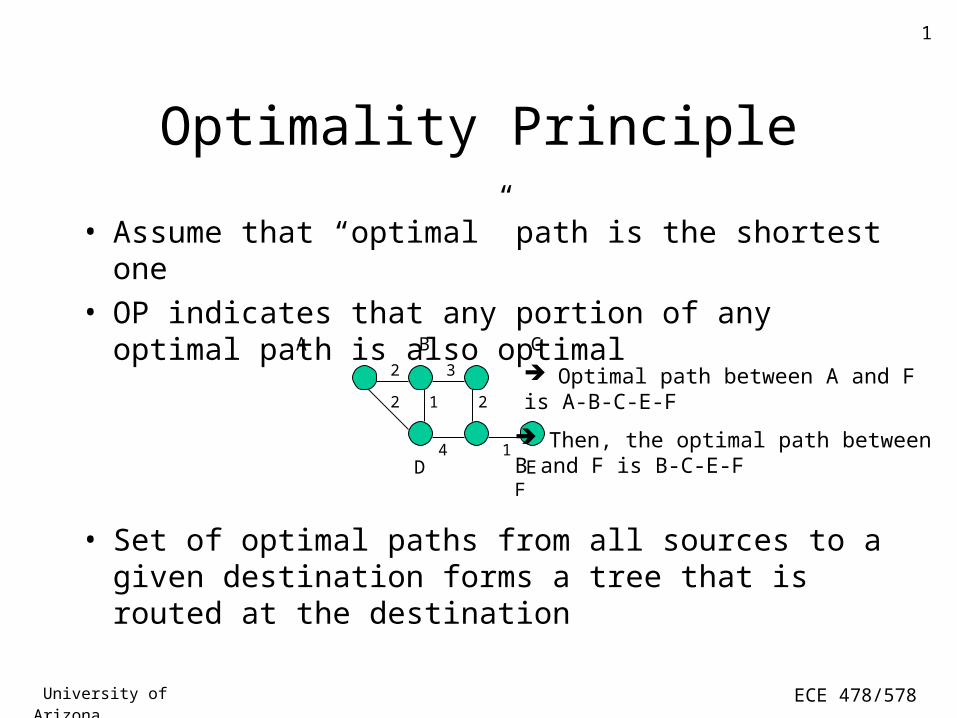
• Assume that “optimal” path is the shortest one

• OP indicates that any portion of any optimal path is also optimal

• Set of optimal paths from all sources to a given destination forms a tree that is routed at the destination

A B C

D E F

2 3

2 1 2

4 1

Optimal path between A and Fis A-B-C-E-F

Then, the optimal path betweenB and F is B-C-E-F


2

Shortest Path Algorithm

• “Shortest” in the sense of distance (e.g., total delay)

• Assume that distance is “additive”

• Two approaches to computing the shortest path:– Dijkstra’s algorithm (basis for link-state routing)

– Bellman-Ford algorithm (basis for distance-vector routing)


3

Dijkstra’s Algorithm

• Goal: find the shortest path from a given source to all destinations

• Network is represented by a graph G(V,E), where– V: set of nodes

– E: set of links (edges)

• Assume that each link is associated with a delay value

• Starting from the source node, the algorithm “discovers” remaining node in the order of their distances from the source


4

Dijkstra’s Algorithm (Cont.)

• Each node v V is associated with a label:– Current best distance from source s to v– Previous node from which distance was obtained

• Initially, all labels are tentative• If the distance is not known yet, it is set to infinity• In each iteration, the algorithm chooses a working

node from set of nodes with tentative nodes– Working node is one with smallest distance among

tentatively labeled nodes– Its label now becomes permanent


5


• Variables:– V: set of nodes in the graph

– s: source node

– dij: link cost from node i to node j (= if i is not a neighbor of j)

– M: set of permanently labeled nodes

– Un: current distance from s to node n


6


• Initialization:– M = {s}, Un = dsn , n s (= if n is not a neighbor of

s)

• Repeat until M = V:– Find working node v V-M such that Uv = min Un

– M = M v (v is permanently labeled)

– Un = min{Un, Uv+ dvn} for all n V-M

• Worst-case complexity is in the order of n2 (although, lower complexities can be achieved)


7

Example


8

Routing in the Internet

• Two general types of routing algorithms

1. Distance-vector

2. Link-state

• Common aspects – Each router knows the address of its neighbors

– Each router knows the cost of reaching its neighbors

– Router obtains global routing information by exchanging information with its neighbors only

distributed routing


9

Routing in the Internet (Cont.)

• Fundamental difference– Distance-vector: a node informs its neighbors of its

“distance” to every other node in the network

– Link-state: a node tells every other node in the network of its “distance” to its neighbors

– Distance can be interpreted in different ways


10

Distance-Vector Algorithm

• Developed by Bellman and Ford

• Each router maintains a distance vector

• Distance vector: list of [destination,cost] pairs– Cost is the cost of the shortest path from the router to a

given destination (initialized to )

• Router periodically broadcasts its distance vector

• When a router receives the distance vector of a neighbor, it updates its own distance vector


11

Example

A B C D

A

Initial

0 1 4 1 0 1 1

1 0 2

1 2 0

B

C

D 4

1 0 1 1

2 1 2 2

0 1 4

0 1 2 2

AB=1

Computation at A whenDV from B arrives

Cost to go to B from A

Cost to destn from B

Cost to destn via B

Current cost from A

MIN

Newcost = New DV for A

+

=

B BNext Hop

A

C

B

D1

41

1

4


12

1 1

Problem with Distance-Vector Routing

• Formation of loops after a link goes down

count-to-infinity problem

B -

A 2 B

B 1 C

A 2 B

B -

A -

B -

A 4 B

B 3 A

A -A B C

COSTTO C

NEXTHOP

INITIAL

1

Link BC GOESDOWN

2

EXCHANGE

3

EXCHANGE

4

EXCHANGE

5

STABLE

Portion of the RT at A

Portion of the RT at B


13

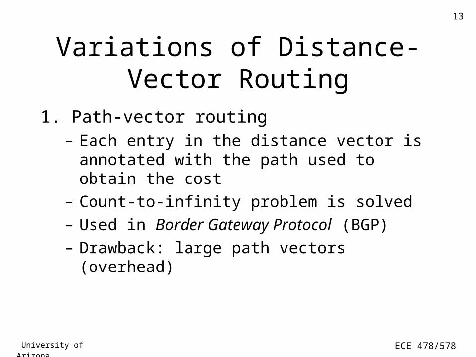
Variations of Distance-Vector Routing

1. Path-vector routing– Each entry in the distance vector is annotated with the

path used to obtain the cost

– Count-to-infinity problem is solved

– Used in Border Gateway Protocol (BGP)

– Drawback: large path vectors (overhead)


14

Variations of Distance-Vector Routing (Cont.)

2. Split-horizon routing– Router does not advertise the cost of a destination to a

neighbor if that neighbor is the next hop to that destination

– Solves count-to-infinity problem for two routers

– Does not work when three or more routers count to infinity

– Variant of split-horizon• split-horizon with poisonous reverse

• used in Routing Information Protocol (RIP)


15

Variations of Distance-Vector Routing (Cont.)

3. Distance-vector with source tracing– In addition to cost to destination, distance vector

includes the address of the router immediately preceding the destination

– Router can construct entire path to destination

– When router updates costs in its distance vector, it also updates preceding-router field


16

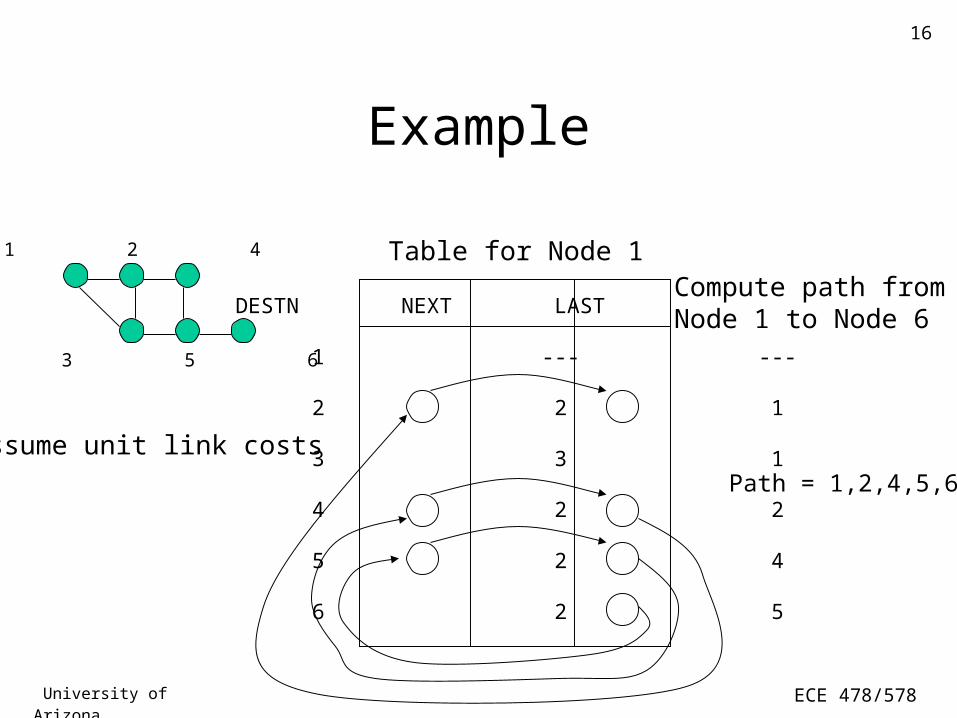
Example

DESTN NEXT LAST

1 --- ---

2 2 1

3 3 1

4 2 2

5 2 4

6 2 5

Path = 1,2,4,5,6

Table for Node 11 2 4

3 5 6

Assume unit link costs

Compute path from Node 1 to Node 6


17

Link-State Routing

• Principles– Each router discovers its neighbors (using “Hello” packets)

– Each router learns the cost of all links in the network (using topology/state dissemination)

– Each router computes the best path to every destination (using Dijkstra's shortest path algorithm)

• Topology dissemination– Routers generate link-state packets (LSPs), which contain

• Router's ID

• Neighbor's ID

• Cost of link to the neighbor


18

Link-State Routing (Cont.)

• LSPs are distributed using controlled flooding– Routers send LSPs to neighboring routers

– Routers maintain copies of LSPs

– Duplicate LSPs are not forwarded


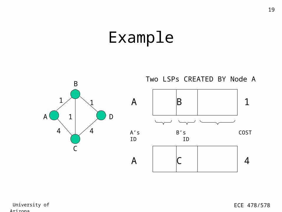
19

Example

C

A D

B

4

1

4

11 A B 1

A C 4

Two LSPs CREATED BY Node A

A’s B’s COSTID ID


20

Example (Cont.)

• A creates two LSPs: A,B,1 and A,C,4• Consider LSP A,B,1• When B receives LSP, it forwards it to C and D

• When C receives LSP from B, it forwards it to A and D

• A does not forward the LSP any further

• If D gets the LSP from B before it gets it from C, it only forwards it to C. Otherwise, it forwards it to B


21

Sequence Numbers in Topology Dissemination

• LSP consistency problem when a link/router goes down

• Solution: use a sequence number for every LSP

• LSP with a higher sequence number overwrites an LSP with lower number

• Wrap-around problem


22

Solutions to Wrap-Around Problem

1. Aging– LSP contains an “age” value

– When LSP is first created, its age is set to MAX_AGE

– When a router receives an LSP, it copies its current age to a per-LSP counter

– Counter is periodically decremented at router

– If age reaches zero, router discards the LSP

2. Lollipop sequence space


23

Link State Versus Distance Vector

• Arguments in favor of link-state algorithms1. Stability (no loops at steady state)

2. Multiple routing metrics can be used

3. Faster convergence than distance vector algorithms

• Counter arguments1. Transients loops can form

2. Modified distance-vector algorithms are also stable and can support multiple metrics


24

Link State Versus Distance Vector (Cont.)

• Arguments in favor of distance-vector algorithms1. Less overhead to maintain database consistency

2. Smaller routing tables

• Counter arguments– These advantages disappear when using modified

distance-vector algorithms (e.g., path vector approach)

• Internet uses both approaches– OSPF: link-state protocol

– BGP: path-vector protocol


25

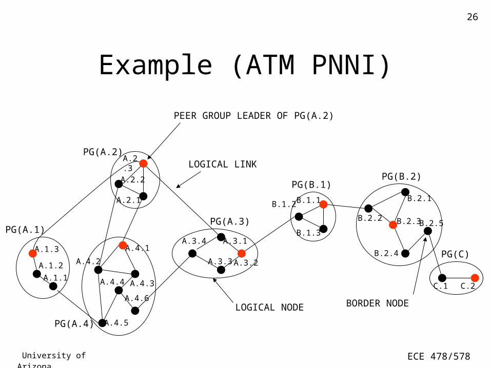
Hierarchical Routing

• For large networks, state dissemination poses a scalability problem

• Solution: cluster routers hierarchically into several peer groups (domains)

• Summarized reachability information is advertised outside a group

• Grouping can be done at multiple levels


26

Example (ATM PNNI)

PEER GROUP LEADER OF PG(A.2)

LOGICAL LINKPG(A.2)

PG(A.1)

PG(A.4)

PG(A.3)

PG(B.1)PG(B.2)

PG(C)

BORDER NODELOGICAL NODE

A.3.1

A.3.2A.3.3

A.3.4

A.2.3

A.2.1

A.2.2

A.1.3

A.1.2

A.1.1

A.4.1

A.4.2

A.4.3A.4.4

A.4.6

A.4.5

B.1.2

B.1.3

B.1.1 B.2.1

B.2.2 B.2.3

B.2.4

B.2.5

C.1 C.2


27

Traffic Management & Control

• Goals: – Guarantee applications QoS requirements

– Provide congestion control

– Utilize resources efficiently

• Above goals sometimes conflict with each other

• Common approach to traffic management:– Map applications QoS into few service classes

– Guarantee QoS associated with these classes


28

How Many Classes of Service?

• One class– Based on the most demanding traffic

– Simple traffic management

– Poor bandwidth utilization

• Many classes – Better utilization

– Traffic management is more complicated


29

1. Reactive control– Action is taken after congestion is detected– Essentially, closed-loop flow control– Network instructs users to reduce their rates

• end-to-end flow control (similar to TCP)• link-by-link flow control

– Problems • Too slow in a high-speed switching environment• Overreaction to temporary congestion• Fairness issues

Types of Traffic Control


30

Types of Traffic Control (Cont.)

2. Preventive control– Prevent the occurrence of congestion by means of

• call admission control (CAC)

• traffic policing (usage parameter control)

– Appropriate for real-time traffic (e.g., voice and video)


31

1. Connection admission control (CAC)

2. Traffic policing and shaping

3. Resource management– Scheduling

– Buffer management

– Priority mechanisms

– Bandwidth allocation

4. Flow control

Traffic Control Functions


32

• Also known as usage parameter control (UPC)

• Goals of UPC: – Ensure compliance with traffic contract

protect QoS of ongoing connections

– Traffic shaping (done by users and/or network)

– User identity verification

• Reasons for traffic violations:– Equipment malfunctioning

– Economical advantage (greedy users)

– Malicious behavior (degrade QoS of others)

Traffic Policing


33

Traffic Policing (Cont.)• Several levels of policing (VC, link, etc.)

• Actions taken when violations are detected– Packet discarding, or

– Packet tagging (marking packets with lower priority)

• Other possible actions at the connection level– Punitive charging

– Connection termination

– Problems with connection-level actions • long reaction time

• drastic penalty


34

Traffic Policing (Cont.)

• Locations at which traffic policing takes place– Entry nodes (network side of user-network interface)

– Boundaries between different networks

• Commonly policed parameters: 1. Peak cell rate (PCR)

2. Sustained cell rate (SCR)

3. Maximum burst size (MBS)


35

Issues in Traffic Policing

• Limitations of current set of traffic parameters

• How do users estimate their traffic parameters?

• Traffic parameters may change within CPE before reaching the policing function

tolerance levels are needed


36

Ideal Requirements in a Policing Mechanism

• Availability

• Online operation

• High probability of detecting violations

• Transparency to conforming connections very low probability of a wrong decision

• Short reaction time


37

• Set of traffic parameters describing a source• Used as basis for traffic contract• Often based on a traffic envelope

– Time-invariant bound on number of arrivals– Often, it represents the worst-case (deterministic) behavior– Also known as “traffic constraint function”– Examples:

• peak rate• (, ) model• linear bounded arrival processes (LBAP)

Traffic Descriptor


38

(,) Traffic Envelope

• Let A[t, t + ] = no. of arrivals in interval [t, t + ]

• Traffic envelope is the function A*() s.t.

A[t, t + ] A*(), t > 0

• In the (,) model, A*() = +

: burstiness parameter

: rate parameter


39

(, ) Traffic Envelope (Cont.)

CumulativeNumberof Arrivals

Window Size

slope =


40

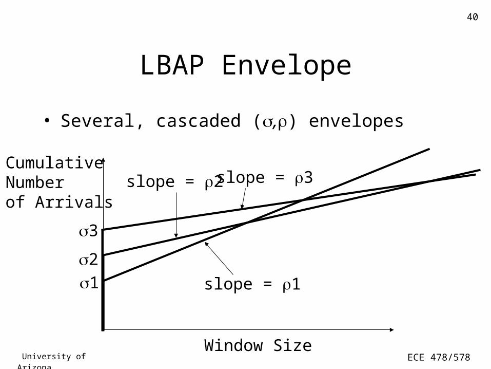
LBAP Envelope

• Several, cascaded (,) envelopes

CumulativeNumberof Arrivals

Window Size

slope = 11

2

3

slope = 2 slope = 3


41

Properties of a good traffic descriptor

1. Representativity

2. Verifiability

3. Preservability

4. Usability


42

Common Policing Mechanisms

1. Leaky bucket

2. Jumping window

3. Moving window

4. Triggered jumping window

5. Exponentially weighted moving average


43

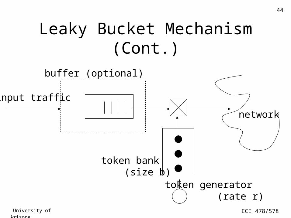
Leaky Bucket Mechanism

• Tokens are generated at rate r

• Token pool of size b (for unused tokens)

• Input buffer (optional)

• For simplicity, assume that packets are of fixed size

• A packet must obtain a token to enter the network

• Output traffic conforms to (, ) envelope

• Can be implemented using two counters


44

Leaky Bucket Mechanism (Cont.)

network

token generator (rate r)

token bank (size b)

buffer (optional)

input traffic


45

Jumping Window Mechanism

• Time is divided into fixed-length windows

• Number of packets per window less than or equal N

• Worst-case burst length = 2N

• Can be implemented using two counters


46

Moving Window Mechanism

• Time window is continuously sliding

• Number of packets per window at any time N

• Each packet is remembered for exactly one window

• Worst-case burst length = N

• Higher implementation complexity than JW


47

Composite Policing Mechanisms

• Previous mechanisms enforce simple envelopes

• To enforce more representative traffic envelopes,

composite policing mechanisms can be used

• A composite mechanism consists of several basic

policing mechanisms connected in cascade

• Example: Composite Leaky Bucket (i.e., LBAP)


48

Composite Leaky Bucket

Window size

AccumulatedNo. of Packets

compliance region

LB1LB2 LB3


49

• Adopted by ATM Forum for traffic policing

• Based on continuous-state leaky bucket

• Characterized by two parameters

– Increment (I)

– Limit (L)

Generic Cell Rate Algorithm (GCRA)


50

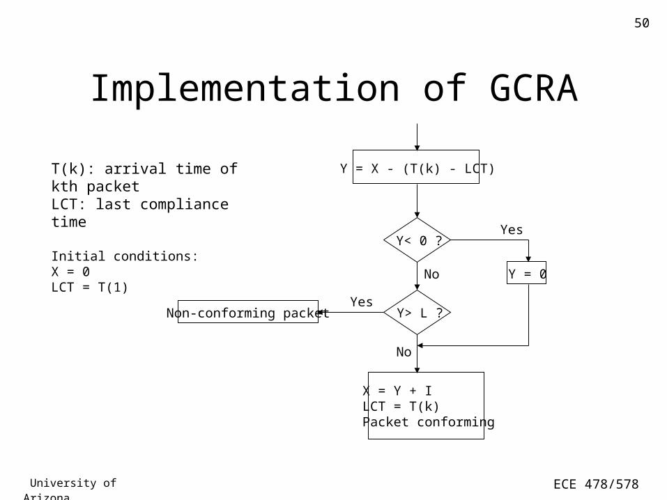
Y< 0 ?

Y = X - (T(k) - LCT)

Non-conforming packet

X = Y + ILCT = T(k)Packet conforming

Yes

No

Y = 0

T(k): arrival time of kth packetLCT: last compliance time

Initial conditions:X = 0LCT = T(1)

Y> L ?Yes

No

Implementation of GCRA


51

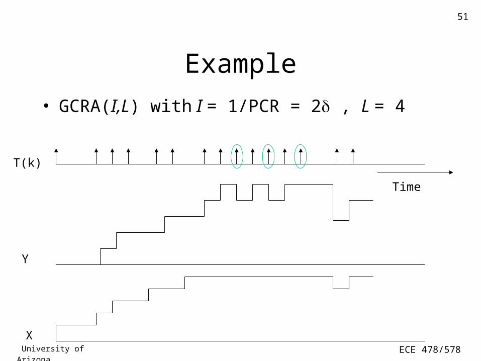
Example

• GCRA(I,L) with I = 1/PCR = 2 , L = 4

Time

T(k)

Y

X

university of arizona ece 478/578 258 optimality principle assume that “optimal” path is the...

Documents

node n slide

working node v v

distancevector algorithm

neighbors distance

university of arizona

distancevector routing

current distance

node i