moral hazard and the optimality of debt - · pdf filemoral hazard and the optimality of debt 3...
TRANSCRIPT
MORAL HAZARD AND THE OPTIMALITY OF DEBT
BENJAMIN HEBERT, STANFORD UNIVERSITY
ABSTRACT. I show that, in a benchmark model, debt securities minimize the welfare losses asso-ciated with the moral hazards of excessive risk-taking and lax effort. For any security design, thevariance of the security payoff is a statistic that summarizes these welfare losses. Debt securitieshave the least variance, among all limited liability securities with the same expected value. In othermodels, mixtures of debt and equity are exactly optimal, and pure debt securities are approximatelyoptimal. I study both static and dynamic security design problems, and show that these two typesof problems are equivalent. I use moral hazard in mortgage lending as a recurring example, but myresults apply to other corporate finance and principal-agent problems.
1. INTRODUCTION
Debt contracts are widespread, even though debt encourages excessive risk taking. In this paper,I show that debt is the optimal security design in a model in which both reduced effort and excessiverisk-taking are possible, even though debt leads to excessive risk taking. In the model, the sellerof the security can alter the probability distribution of outcomes in arbitrary ways. This allows theseller to both alter the mean value of the outcome (“effort”) and change the other moments of thedistribution of outcomes (“risk-shifting”). To minimize the welfare losses arising from this moralhazard, the security’s payout must be designed to minimize variance. Debt securities are optimalbecause, among all limited-liability securities with the same expected value, they have the leastvariance.
The model is motivated by settings in which debt contracts are prevalent and both reduced effortand risk-shifting are possible. For example, in residential mortgage origination, lenders mightbe able to both underwrite loans more or less diligently (effort) and use private information tochoose more or less risky borrowers (risk-shifting). Prior to the 2008 financial crisis, mortgage
Key words and phrases. security design, moral hazard, optimal contracts.Acknowledgments: I would like to thank, in no particular order, Emmanuel Farhi, Philippe Aghion, Alp Simsek, DavidLaibson, Alex Edmans, Luis Viceira, Jeremy Stein, Yao Zeng, John Campbell, Ming Yang, Oliver Hart, David Scharf-stein, Sam Hanson, Adi Sunderam, Guillaume Pouliot, Yuliy Sannikov, Zhiguo He, Lars Hansen, Roger Myerson,Michael Woodford, Gabriel Carroll, Drew Fudenberg, Scott Kominers, Eric Maskin, Mikkel Plagborg-Møller, BengtHolmstrom, Arvind Krishnamurthy, Peter DeMarzo, Sebastian Di Tella, and many seminar participants for helpfulfeedback. I would also like to thank Dimitri Vayanos (the editor) and three anonymous referees for comments thathelped improve the paper. A portion of this research was conducted while visiting the Becker Friedman Institute. Allremaining errors are my own. Email: [email protected].
1

MORAL HAZARD AND THE OPTIMALITY OF DEBT 2
lenders sold debt securities, backed by mortgage loans, to outside investors. The issuance of thesesecurities may have weakened the incentives of mortgage lenders to lend prudently. Despite thiseffect, I argue that debt can be optimal, because debt securities balance the need to encourage effortwith the need to avoid risk-shifting.
Many elements of the model are standard in the security design literature. The security is theportion of the asset value received by the outside investors, and is subject to limited liability con-straints. If the seller retains a levered equity claim, she1 has sold a debt security. There are gainsfrom trade, meaning that the outside investors value the security more than the seller does, holdingthe distribution of outcomes fixed. Both the outside investors and the seller are risk-neutral.
The key non-standard element of the model is a flexible form of moral hazard, which builds onthe work of Holmstrom and Milgrom (1987). The seller, through her actions, can create a “zero-cost” distribution of outcomes, which she will do if she has no stake in the outcome. If the sellercreates any other probability distribution, she incurs a cost. In my benchmark model, the cost to theseller of choosing a probability distribution p is proportional to the Kullback-Leibler divergence(or “relative entropy”) of p from the zero-cost distribution. Under this assumption, the combinedeffects of reduced effort and risk-shifting can be summarized by one statistic, the variance of thesecurity payoff. The gains from trade are proportional to another statistic, the mean security payoff.Debt securities maximize mean-variance tradeoffs over the set of limited liability securities, andare therefore optimal in this benchmark model.
Minimizing the variance of the security payoff is equivalent to making the security “as flat aspossible.” Intuitively, if the security pays the buyer more in state i than in state j, the seller willinefficiently act to ensure that state i is less likely than state j. Reducing the security payoffin state i and increasing it in state j would cause the seller to increase the likelihood of state irelative to state j, benefitting the buyer. Completely flat securities would be best, but becauseof the limited liability constraints, the security can only be completely flat if it pays nothing atall and foregoes all of the gains from trade. Debt securities are the optimal compromise: theyhave positive expected value, capturing some gains from trade, but are flat wherever possible,minimizing inefficient actions by the seller.
I also analyze larger classes of cost functions. When the cost function is not the KL divergence,but instead another α-divergence, the optimal security designs exist on a continuum, with the “live-or-die” security of Innes (1990) at one end (see the appendix, Figure A.1), equity at the other, anddebt in the middle. In some cases, the security design is upward sloping, and can be thought of as
1Throughout the paper, I will use she/her to refer to the seller and he/his to the buyer of the security. No association ofthe agents to particular genders is intended.
MORAL HAZARD AND THE OPTIMALITY OF DEBT 3
a mix of equity and debt. In other cases, the optimal security design is downward sloping. In thesecases, restricting security designs to be monotone for the buyer restores the optimality of debt.
Both the KL divergence and the other α-divergences are part of a broader class of divergences,the invariant divergences. For this class of divergences, I show that debt securities, and mixturesof debt and equity, are approximately optimal. The approximation I use applies when the moralhazard and gains from trade are small relative to scale of the assets. It is appropriate in settingsin which the difference, in utility terms, between a well-designed contract and a poorly designedcontract is comparable to the seller’s “value added.” I describe the approximation in more detail,and discuss when it is and is not appropriate, in section §5. Under this approximation, debt is first-order optimal, meaning that debt securities are a detail-free way to achieve nearly the same utilityas the optimal security design. Mixtures of debt and equity, which correspond to the optimalcontracts for α-divergences, are second-order optimal for all invariant divergences. This can beinterpreted as a “pecking order,” in which the security design grows more complex as the size ofboth the moral hazard problem and gains from trade grow, relative to the scale of the assets.
Finally, I provide a micro-foundation for the security design problem with the KL divergencecost function, using a dynamic model. I show that a continuous-time moral hazard problem, similarto Holmstrom and Milgrom (1987), is equivalent to the static moral hazard problem. The equiva-lence of the static and dynamic problems provides an intuitive explanation for how the seller cancreate any probability distribution of outcomes. The key distinction between the dynamic modelsI discuss and the principal-agent models of Holmstrom and Milgrom (1987) is limited liability. InHolmstrom and Milgrom (1987), linear contracts for the seller (agent) are optimal, because theyinduce the seller to take the same (efficient) action each period. In my model, because of limitedliability, the only way to implement the efficient action at every state and time is to offer the sellera very large share of the asset value. However, offering the seller a large share of the asset valuelimits the gains from trade. It is preferable to pay the seller nothing in the worst states of the world,and then at some point offer a linear payoff. Even though this design does not induce the seller totake the efficient action at every state and time, it achieves more gains from trade. The design forthe retained tranche that I have just described, levered equity, corresponds to selling a debt security.
This optimality of debt in my benchmark model illustrates a key distinction between my modeland the existing security design literature. The classic paper of Jensen and Meckling (1976) arguesthat debt securities are good at providing incentives for effort, but create incentives for risk-shifting,while equity securities avoid risk-shifting problems, but provide weak incentives for effort. A nat-ural conjecture, based on these intuitions, is that when both risk-shifting problems and effort incen-tives are important, the optimal security will be “in between” debt and equity. In my benchmarkmodel, contrary to this intuition, a debt security is optimal.
MORAL HAZARD AND THE OPTIMALITY OF DEBT 4
The argument of Jensen and Meckling (1976) that debt is best for inducing effort relies on arestriction to monotone security designs. The “live-or-die” result of Innes (1990) shows that whenthe seller can supply effort to improve the distribution of outcomes (in a monotone likelihoodratio property sense), it is efficient to give the seller all of the asset value when the asset valueis high, and nothing otherwise. A revised intuition, which I formalize in section §4, is that thesecurities (including debt) that optimally balance encouraging effort and avoiding risk-shifting are“in between” the live-or-die security and equity.2
The benchmark model in this paper takes the idea of flexibility in moral hazard problems to anextreme, allowing the seller to create any probability distribution of outcomes, subject to a cost.This approach to moral hazard problems was introduced by Holmstrom and Milgrom (1987). It isconceptually similar to the notion of flexible information acquisition, emphasized in Yang (2015).3
However, in this paper, the cost of choosing a probability distribution should be interpreted asa cost associated with the actions required to cause that distribution to occur (underwriting ornot underwriting mortgage loans, for example). In the rational inattention literature, which Yang(2015) builds on, gathering or processing information (as opposed to taking actions) is costly. Thisdistinction is blurred in the rational inattention micro-foundation in the online appendix, section §2.
In contrast, much of literature on security design with moral hazard allows the seller to controlonly one or two parameters of the probability distribution. These papers do not find that debt isoptimal. In Acharya et al. (2016), bank managers can both shift risk and pursue private benefits, butdo this by choosing amongst three possible investments. In Edmans and Liu (2010), who argue thatis efficient for the agent (not the principal) to hold debt claims, also have a binary project choice.Closer to this paper is Biais and Casamatta (1999), in which there are three possible states andtwo levels of effort and risk-shifting. Biais and Casamatta (1999) interpret the optimal contractsover those three states as mixtures of debt and equity. Hellwig (2009) has a two-parameter modelwith continuous choices for risk-shifting and effort, and finds that a mix of debt and equity areoptimal. In his model, risk-shifting is costless for the agent. Fender and Mitchell (2009) have amodel of screening and tranche retention, which is a single-parameter model. This paper differsfrom this literature by allowing for arbitrary outcome spaces, arbitrary probability distributions,and continuous moral hazard choices, which makes deriving general results difficult (Grossmanand Hart (1983)), and by considering flexible models of moral hazard. In the online appendix,section §1, I discuss how to extend my results to parametric models, relating the framework Idevelop to this literature.
2A similar result, derived from a robust contracting framework, appears in Antic (2015).3This paper also builds on some of the methods of Yang (2015) (see the appendix, section 3.15).

MORAL HAZARD AND THE OPTIMALITY OF DEBT 5
Innes (1990) advocates a moral-hazard theory of debt, but debt is optimal only when the sellercontrols a single parameter, and the security is constrained to be monotone. If the security doesnot need to be monotone, or if the seller controls both the mean and variance of a log-normaldistribution, the optimal contract is not debt.4 In the corporate finance setting, one argument formonotonicity is that a manager can borrow from a third party, claim higher profits, and then repaythe borrowed money from the extra contract payments. In addition to the accounting and legal bar-riers to this kind of “secret borrowing,” the third party might find it difficult to force repayment. Inthe context of asset-backed securities, where cash flows are more easily verified, secret borrowingis even less plausible. Another argument in favor of monotonicity concerns the possibility of thebuyer (principal, outside shareholders) sabotaging the project. In the context of securitization, thebuyer exerts minimal control over the securitization trust and sabotage is not a significant concern.
There is a large literature that justifies debt for reasons other than moral hazard. Papers invokingadverse selection include Nachman and Noe (1994), DeMarzo and Duffie (1999), Dang et al.(2011), Vanasco (2016) , and Yang (2015). In unreported results, I find that the benchmark modelof this paper and of Yang (2015) can be combined to produce debt as the optimal contract, whereasother parametric models of moral hazard, when combined with Yang (2015), would not generallyresult in debt. Other theories of debt include costly state verification (Townsend (1979); Gale andHellwig (1985)) and explanations based on control or limiting investment (Aghion and Bolton(1992), Jensen (1986), Hart and Moore (1994)).
I begin in section §2 by explaining the benchmark security design problem, whose structureis used throughout the paper. I then show in section §3 that for a particular cost function, debtis optimal, and explain how this relates to a mean-variance tradeoff. Next, I analyze other costfunctions in section §4, describing the optimal contracts and showing a related mean-variancetradeoff applies. I will then introduce an approximation in section §5, and show that for an evenlarger class of cost functions, the same tradeoffs hold in an approximate sense. In section §6 andsection §7, I provide micro-foundations for the non-parametric models, from a continuous timemodel. In the appendix, section §C, I discuss a calibration for the example of residential mortgagelending. In the online appendix, section §1, I discuss parametric models, and apply the results inonline appendix section §2 to a model of rational inattention in mortgage lending.
2. MODEL FRAMEWORK
In this section, I introduce the security design framework that I will discuss throughout the paper.The problem is close to Innes (1990) and other papers in the security design literature. There is arisk-neutral agent, called the “seller,” who owns an asset in the first period. In the second period,
4For brevity, I have omitted the result for log-normal distributions from the paper. It is available upon request.

MORAL HAZARD AND THE OPTIMALITY OF DEBT 6
one of N + 1 possible states, indexed by i ∈ Ω = 0, 1, . . . , N, occurs.5 In each of these states,the seller’s asset has an undiscounted value of vi. I assume that v0 = 0, vi is non-decreasing in i,and that vN > v0.
The seller discounts second period payoffs to the first period with a discount factor βs. Thereis a second risk-neutral agent, the “buyer,” who discounts second period payoffs to the first periodwith a larger discount factor, βb > βs. Because the buyer values second period cash flows morethan the seller, there are “gains from trade” if the seller gives the buyer a second period claim inexchange for a first period payment. I will refer to the parameter κ = βb−βs
βsas the gains from
trade.6
I assume there is limited liability, so that in each state the seller can credibly promise to pay atmost the value of the asset. I also assume that the seller must offer the buyer a security, meaningthat the second period payment to the buyer must be weakly positive. In this sense, the seller mustoffer the buyer an “asset-backed security.” When the asset takes on value vi in the second period,the security pays si ∈ [0, vi] to the buyer. Following the conventions of the literature, I will saythat the security is a debt security if si = min(vi, v) for some v ∈ (0, vN).
To simplify the exposition, I make particular assumptions about the timing of the events and thebargaining power of the agents. I will assume that, during the first period, the seller first designs thesecurity, and then makes a “take-it-or-leave-it” offer to the buyer at priceK. If the buyer rejects theoffer, the seller retains the entire asset. After the buyer accepts or rejects the offer, the seller takesactions that modify the value of the assets (the moral hazard). The first period ends, uncertainty isresolved, and then in the second period payoffs are determined.
This timing convention, which is standard in principal-agent models, is not appropriate for someapplications. For example, in mortgage origination, much of the lender’s moral hazard occurswhen the loans are being underwritten, before they are sold to outside investors. In the appendix,section §B, I show that this timing of events is not necessary for the main results. This robustnessto the timing of events contrasts with models based on adverse selection by the seller, such asDeMarzo and Duffie (1999), in which the timing of events is crucial. In the same appendix section,I also show that allowing the buyer and seller to Nash-bargain over the price, or over both the priceand security design, does not alter the main results.
The moral hazard problem occurs when the seller creates or modifies the asset. During thisprocess, the seller will take a variety of actions, and these actions will alter the probability dis-tribution of second period asset values. Following Holmstrom and Milgrom (1987), I model theseller as directly choosing a probability distribution, p, over the sample space Ω, subject to a cost
5Using a discrete outcome space simplifies the exposition, but is not necessary for the main results.6The gains from trade could also be motivated by a requirement that the seller raise a certain amount of funds from thebuyer (see appendix section §B).

MORAL HAZARD AND THE OPTIMALITY OF DEBT 7
ψ(p). I will focus models in which any probability distribution p can be chosen, which I will call“non-parametric.” In appendix section §1, I discuss models in which p must belong to a parametricfamily of distributions.7
I will make several assumptions about the cost function ψ(p). First, I assume that there is aunique probability distribution, q, with full support over Ω, that minimizes the cost. Second, be-cause I will not consider participation constraints for the seller, I assume without loss of generalitythat ψ(q) = 0. I also assume that ψ(p) is strictly convex and at least twice differentiable. Below,I will impose additional assumptions on the cost function, but first will describe the moral hazardand security design problems.
The moral hazard occurs because the seller cares only about maximizing the value of her payoff.When the value of the asset is vi, the discounted value of the seller’s retained tranche is
ηi = βs(vi − si).
Because of the assumption that v0 = 0, and limited liability, it is always the case that η0 = s0 = 0.Let pi denote the probability that state i ∈ Ω occurs, under probability distribution p. The moralhazard sub-problem of the seller can be written as
(2.1) φ(η) = supp∈M∑i>0
ηipi − ψ(p),
where M is the set of feasible probability distributions and φ(η) is the indirect utility function. Inthe non-parametric case, when M is the set of all probability distributions on the sample space, themoral hazard problem has a unique optimal p for each η. Moreover, the smoothness and convexityof ψ(p) guarantee that this optimal policy, p(η), is itself differentiable with respect to η. In contrast,for the parametric case (appendix section §1), there may be multiple p ∈ M that achieve the sameoptimal utility for the seller.
The buyer cannot observe p directly, but can infer the seller’s choice of p from the design of theretained tranche η. At the security design stage, the buyer’s valuation of a security s is determinedby both the structure of the security and the buyer’s inference about which probability distributionthe seller will choose, p(η). Without loss of generality, I will define the units of the seller’s andbuyer’s payoffs so that βs
∑i vip
i(βsvi) = 1. That is, if the seller retains the entire asset, andtakes actions in the moral hazard problem accordingly, the discounted asset value is one. I use thisconvention to ensure that the units correspond to a quantity that is at least potentially observable:the value of the assets, if those assets are retained by the seller. This convention is useful in thecalibration of the model in the appendix, section §C.7Because the sample space Ω is a finite set of outcomes, even in the “non-parametric” case, the choice of p can beexpressed as a choice over a finite number of parameters. I am using the terms non-parametric and parametric todenote whether the set M of feasible probability distributions is the entire simplex, or a restricted set.

MORAL HAZARD AND THE OPTIMALITY OF DEBT 8
Let si(η) be the security corresponding to retained tranche η. The security design problem is
(2.2) U(η∗) = maxηβb
∑i>0
pi(η)si(η) + φ(η),
subject to the limited liability constraint that ηi ∈ [0, βsvi]. From the seller’s perspective, when sheis designing the security, she internalizes the effect that her subsequent choice of p will have on thebuyer’s valuation, because that valuation determines the price at which she can sell the security.The security serves as a commitment device for the seller, providing an incentive for her to choosea favorable p. This commitment is costly, because allocating more of the available asset value tothe retained tranche necessarily reduces the payout of the security, reducing the gains from trade.
Many of the results in this paper are discussed using perturbation arguments. Any infinitesimalperturbation to the security design (and therefore retained tranche) has two effects on the seller’sutility in the security design problem. The first effect is the “direct” effect, which changes theseller’s utility by transferring more or less expected value from the seller to the buyer. In general,the size of this effect is controlled by the gains from trade parameter, κ. The second effect is the“indirect” effect, which changes the buyer’s valuation of the security, through the change in theseller’s behavior in the moral hazard problem. There is no “indirect” effect on the seller’s utility inthe moral hazard problem, because the seller is maximizing her utility in the moral hazard problemwhen she chooses the probability distribution (the envelope theorem).
Consider a differentiable perturbation around the optimal security design, η(ε), with η(0) = η∗,that is feasible for some ε > 0. As mentioned above, in the non-parametric models that I study,p(η) is differentiable. In this case, the two effects of a perturbation can be summarized by thefollowing first-order optimality condition with respect to ε, the size of the perturbation:
(2.3)∂U(η(ε))
∂ε|ε=0+ = −κ
∑i∈Ω
pi(η∗)∂ηi∂ε|ε=0+︸ ︷︷ ︸
direct effect
+ βb∑i,j∈Ω
s∗j∂pj(η)
∂ηi|η=η∗
∂ηi∂ε|ε=0+︸ ︷︷ ︸
indirect effect
≤ 0.
Below, I will further decompose the indirect effect into an indirect effect due to a change in effortand an indirect effect due to a change in risk-shifting. First, however, I will describe the costfunctions that I will be studying in more detail.
As discussed earlier, the cost function ψ(p) is convex and minimized at ψ(q) = 0. It followsthat the cost function is proportional to a divergence8 between p and the zero-cost distribution, q,defined for all p, q ∈M :
ψ(p) = θD(p||q).8A “divergence” is similar to a distance, except that there is no requirement that it be symmetric between p and q, orthat it satisfy the triangle inequality.

MORAL HAZARD AND THE OPTIMALITY OF DEBT 9
Here, the scalar parameter θ > 0 controls how costly it is for the seller to change the probabilitydistribution in the moral hazard problem. I introduce this parameter for the purpose of takingcomparative statics.
There are many divergences that have been defined in the information theory literature (e.g. Aliand Silvey (1966), Csiszar (1967), Amari and Nagaoka (2007)). In section §3, I begin the paperby focusing on a particular divergence, the Kullback-Leibler divergence. The KL divergence, alsocalled relative entropy, is defined as
DKL(p||q) =∑i∈Ω
pi ln(pi
qi).
The KL divergence has the assumed convexity and differentiability properties, and also guaranteesthat the p chosen by the seller will be mutually absolutely continuous with respect to q. The KLdivergence has been used in a variety of economic models, notably Hansen and Sargent (2008),who use it to describe the set of models a robust decision maker considers. It also has manyapplications in econometrics, statistics, and information theory, and the connection between thesecurity design problem and these topics will be discussed later in the paper. I will show that whenthe cost function is proportional to the KL divergence, debt is the optimal security design.
The KL divergence is a member of the family of α-divergences. These divergences are parametrizedby a real number, α, which controls how the curvature of the divergence changes as p moves awayfrom q. The α-divergences can be written, whenever |α| 6= 1, as
Dα(p||q) =∑i∈Ω
4
1− α2qi(1− (
pi
qi)12
(1−α) +1
2(1− α)(
pi
qi− 1)).
The limits of α → −1 and α → 1 correspond to the KL divergence and the “reversed” KLdivergence, respectively.9 For this class of divergences, in section §4 I will show that, for α ≤ −1,the optimal contracts are mixtures of debt and equity. Commonly discussed α-divergences includethe Hellinger distance (α = 0) and the χ2-divergence (α = −3).
I will also discuss a more general class of divergences, that contains the α-divergences, knownas the “f -divergences” . This class of divergences can be written as
(2.4) Df (p||q) =∑i∈Ω
qif(pi
qi),
where f(u) is a convex function on R+ with f(1) = 0. I adopt the convention (without loss ofgenerality) that f(u) ≥ 0.10 I will limit my discussion to sufficiently differentiable f -functions,
9Other authors use different sign conventions or scaling for the α parameter.10Under this convention, the KL divergence corresponds to f(u) = u lnu− u+ 1.

MORAL HAZARD AND THE OPTIMALITY OF DEBT 10
for mathematical convenience, and use the normalization that f ′′(1) = 1. The f -divergences areanalytically convenient because they are additively separable (or “decomposable”) across states.
The most general class of divergences that I will discuss are the “invariant divergences,” whichcontain the f -divergences, along with other divergences that are not additively separable, such asthe Chernoff and Bhattacharyya distances. Invariant divergences are defined by their invariancewith respect to sufficient statistics (Chentsov (2000), Amari and Nagaoka (2007)).The exact defi-nition of an invariant divergence is rather technical; for our purposes, what is special about thesedivergences is that, up to second order, they resemble the KL divergence, and up to third order,they resemble the α-divergences. In section §5, I will define this “resemblance” more precisely,and define how a security design can be “approximately optimal.” I will then show that debt, ormixtures of debt and equity, are approximately optimal as a result.
To summarize, the divergences I discuss are related in the following way:
KL ∈ α-divergences ⊂ f -divergences ⊂ Invariant Divergences ⊂ All Divergences.
The KL divergence, and the broader class of invariant divergences, are interesting because they areclosely related to ideas from information theory. In the appendix, section §2, I illustrate this in amodel based on rational inattention (Sims (2003)), in which the cost function is related to the KLdivergence. The KL divergence cost function can also be micro-founded from a dynamic moralhazard problem. In section §6, I show that a large class of continuous time problems are equivalentto the static moral hazard problem with a divergence cost function, and show that in a particularcase, that divergence is the KL divergence. In section §7, I extend this analysis to a more generalclass of continuous time problems and show that they are related, in a certain sense, to static moralhazard problems with invariant divergence cost functions.
I will refer throughout the paper to “effort” and “risk-shifting” as separate components of themoral hazard problem. Next, I will define “effort” and “risk-shifting” formally, and clarify the con-nection between this framework and more conventional models of moral hazard. I define “effort”as the change in the discounted expected value of the assets:
e = βs∑i∈Ω
(pi − qi)vi.
Given a retained tranche η, define the effort it induces as e(η). For any η, there is an “equivalent eq-uity share”, γ(η), for the seller that would induce the same amount of effort: e(η) = e(γ(η)βsv).11
11This equity share is not necessarily feasible– if η induces a very high or very low level effort, the equivalent equityshare might be more than 100% or less than 0% of the asset value. The probability distribution associated with theequivalent equity contract, p(γ(η)βsv), has the lowest cost among all probability distributions with the same effortlevel.

MORAL HAZARD AND THE OPTIMALITY OF DEBT 11
In the model of Innes (1990), the seller is restricted to choosing from a family of probabilitydistributions that satisfy a monotone likelihood ratio property. As a result, effort, defined in thisway, is one-to-one with the choice variable in Innes (1990). In models with more flexible moralhazard, effort is not one-to-one with the choices of the agent. In these models, we can define “risk-shifting” as the actions that the agent takes which change the probability distribution of outcomeswithout changing the expected value of asset. This includes actions that change the higher mo-ments of the asset distribution, and also actions that keep the distribution of asset values constant,but move probability between states with the same asset value (i, j ∈ Ω with vi = vj). Usingthese definitions of effort and risk-shifting, I decompose the indirect effect of any security designperturbation (equation (2.3)) into effort and risk-shifting components.
Lemma 1. The indirect effect of any security design perturbation can be decomposed into an effectdue to the change in effort, and an effect due to the change in risk shifting:
βb∑j∈Ω
s∗jdpj(η(ε))
dε|ε=0+︸ ︷︷ ︸
indirect effect
=βbβs
(1− γ(η∗))de(η(ε))
dε|ε=0+︸ ︷︷ ︸
indirect effect on effort
−
βbβs
∑j∈Ω
dpj(η(ε))
dε|ε=0+(η∗j − γ(η∗)βsvj)︸ ︷︷ ︸
indirect effect on risk shifting
.
Proof. See online appendix, section 3.1.
This decomposition is not unique; there are many other ways of decomposing the indirect ef-fects into different components. This particular decomposition connects the flexible moral hazardframework used in this paper to other models of moral hazard. Using this definition of effort andrisk-shifting, an equity contract causes no utility loss due to risk-shifting, because an equity con-tract is identical to its “equivalent equity” contract, consistent with the argument of Jensen andMeckling (1976). However, equity contracts might not be a very efficient way to induce effort bythe seller. If the effort level is one-to-one with the seller’s choices (as in Innes (1990)), there is nopossibility of risk-shifting, and this framework reduces to the classic model of moral hazard.
Moral hazard models with two choice parameters, such as Hellwig (2009), allow the seller torisk-shift in one dimension, while also incorporating an effort choice. The non-parametric model ofmoral hazard emphasized in this paper extends these models by allowing more dimensions of risk-shifting. In models with only one dimension of risk-shifting, if there are many possible outcomes(i.e. more than the three in Biais and Casamatta (1999)), there will in general be contracts otherthan equity contracts that also induce no risk-shifting. In contrast, in the non-parametric model ofmoral hazard, equity contracts are the only contracts that avoid risk-shifting entirely.

MORAL HAZARD AND THE OPTIMALITY OF DEBT 12
The decomposition also illustrates the externalities associated with the seller’s choices in themoral hazard problem. The buyer benefits from an increase in the seller’s effort, assuming thatthe seller’s equivalent equity share is less than one hundred percent. At the same time, the buyercan benefit or be harmed by the change in the seller’s risk shifting behavior, depending on whetherthe change in the security design induces more or less risk shifting. I will show in the followingsections that the effect of a perturbation to the security design on risk shifting depends on whetherthe security becomes more or less equity-like.
The models described in the paper use divergences to create cost functions, which rules out twointeresting cases: free disposal of output by the seller, and free risk-shifting. Free disposal of outputby the seller is a common assumption in security design problems, and is used to justify restrictingthe set of securities to designs for which the seller’s payoff is weakly increasing in the asset value.Free disposal of output does not change any of the results in the paper– all of the optimal securitydesigns without free disposal have monotone payoffs for the seller, and are therefore still optimalamong the set of monotone security designs. I discuss this more in the appendix, section §D.
Free risk-shifting is the assumption that only effort, and not risk-shifting, is costly for the agent.Formally, this would require that D(p||q) = D(p′||q) for all p, p′ with the same expected value.Technically, the assumptions of strict convexity forD(p||q) and thatD(p||q) = 0 only if p = q bothrule out this case. However, the analysis in this case is straightforward. As risk-shifting becomesfree, concerns about risk-shifting dominate concerns about effort, and equity contracts are optimal.This result is closely related to Ravid and Spiegel (1997), Carroll (2015), and Barron et al. (2017),and is also shown in the appendix, section §D.
In this section, I have introduced the framework that I will use throughout the paper. In the nextsection, I analyze the benchmark model, in which the cost function is the KL divergence.
3. THE BENCHMARK MODEL
In this section, I discuss the non-parametric version of the model, in which the set M of feasibleprobability distributions is the set of all probability distributions on Ω. I assume that the costfunction is proportional to the KL divergence between p and q,
ψ(p) = θDKL(p||q).
I will show that the optimal security design is a debt contract. In the text, I will outline theproof, using a perturbation argument; a complete proof can be found in the appendix, section 3.5.12
I will start by discussing the first-order condition of the moral hazard problem. The KL divergencecost function becomes infinitely sloped at the boundaries of the simplex, and therefore guarantees
12This perturbation argument builds on the suggestions of an anonymous referee.

MORAL HAZARD AND THE OPTIMALITY OF DEBT 13
an interior solution to the moral hazard problem, equation (2.1), for all η. The KL divergence isalso convex, consistent with the assumptions described in the previous section. As a result, thefirst-order condition in the moral hazard problem must hold. For any i > 0, we have
ηi = θ(ln(pi
qi)− ln(
p0
q0)).
Intuitively, if the seller receives a high payoff in state i, she will increase the probability of state irelative to state 0, in which she receives zero payoff.
From this first-order condition, we can observe that the semi-elasticities of the relative probabil-ities pi(η) and p0(η) to the payoff ηi satisfy
(3.1)∂ ln(pi(η))
∂ηi− ∂ ln(p0(η))
∂ηi= θ−1.
This constant difference of semi-elasticities property is part of what is special about the KL diver-gence. It is constant in two respects; first, the difference of the elasticities does not depend on howfar p(η) is from q, and second, it is symmetric across the states i ∈ Ω. The α-divergences that willbe discussed in the next section relax the first of these properties– the elasticity will depend on howfar the endogenous probability distribution is from the zero-cost distribution. The entire class ofinvariant divergences, which are used throughout the paper, share the second property, imposing asort of symmetry across states of the world (this is essentially the meaning of “invariant”).
Using this property, we can construct perturbations of the retained tranche (and therefore thesecurity design) that changes the probability in two different states, pi and pj , with i > 0 andj > 0, while leaving all other probabilities unchanged. Let η∗ be the optimal design for the retainedtranche. Suppose that, starting from η∗, we increase ηi by an amount ε
pi(η∗), while decreasing ηj by
an amount εpj(η∗)
. Conjecture that this perturbation, for infinitesimal values of ε, increases pi anddecreases pj by θ−1ε, while leaving all other probabilities, and in particular p0, unchanged. We canverify this conjecture by observing that equation (3.1) above is satisfied for all states, and that thesum of the probabilities across states remains equal to one.
Having constructed this perturbation, I now turn to the security design problem. Consider thefollowing property of debt: for a security s to be a debt, there must be no pairs si and sj , withi 6= j, such that sj < vj and sj < si. This property requires that if the limited liability constraintdoes not bind in either state i or state j, the security values must be equal, and if the constraintbinds only in one of the two states, the payoff in that state must be smaller than in the “flat” part ofthe debt contract. It is essentially the definition of a debt contract, subject to the caveat that “sellingeverything” and “selling nothing” also have this property.
Suppose that the optimal security design s∗ does not have this property (and therefore is notdebt). For this to be true, there must be no perturbation of the security design that is feasible and
MORAL HAZARD AND THE OPTIMALITY OF DEBT 14
can improve the seller’s utility in the security design problem. Using the perturbation describedabove, I will show that such a perturbation does exist, and therefore that the optimal contract is adebt (or selling everything/nothing, which are ruled out in the proof in the appendix).
We have supposed that, for the optimal security design s∗, there is a pair of states i, j ∈ Ω, i 6= j,with s∗j < vj and s∗j < s∗i . Now imagine that we increase sj by β−1
sε
pj(η∗)while decreasing si by
β−1s
εpi(η∗)
. The values of the retained tranche in those states, ηi and ηj , move opposite the securitydesign and are perturbed in exactly the manner discussed above. Note that, because s∗j < vj ands∗i > s∗j ≥ 0, this perturbation does not violate the limited liability constraints.
The effect of this perturbation on the utility in the security design problem is described by equa-tion (2.3) in the previous section. We can see that there is no “direct effect” of this perturbation;holding the probability distribution the seller chooses fixed, the perturbation does not affect theexpected value of the security design. The perturbation does increase the probability of state i byθ−1ε, and it decreases the probability of state j by θ−1ε, leaving the probability of all other statesthe same. Therefore, the “indirect” effect is θ−1(s∗i − s∗j), which was assumed to be greater thanzero. It follows that this perturbation improves the seller’s utility, and therefore the optimal con-tract must be a debt, selling everything, or selling nothing. This argument can be summarized asshowing that the security design should be “flat wherever possible.”
After introducing the formal result, I will apply the decomposition between effort and risk-shifting introduced in the previous section. The following proposition summarizes this perturbationargument, rules out selling everything and selling nothing, and also establishes a result about theface value of the debt contract.
Proposition 1. In the non-parametric model, with the cost function proportional to the Kullback-Leibler divergence, the optimal security design is a debt contract,
s∗j = min(vj, v),
for some v > 0. The face value of the debt satisfies
βbv − βb∑i∈Ω
pi(η∗)s∗i = κθ.
If the highest possible asset value is sufficiently large (vN >∑
i qivi + κ
βbθ), then v < vN .
Proof. The results are proven in the proof of proposition 3.
The result in proposition 1 shows that debt is optimal, for any full-support zero-cost distributionq. The condition that vN be “high enough” is weak. If it was not satisfied for some sample spaceΩ and zero-cost distribution q, one could include a new highest value vN+1 in Ω, occurring with

MORAL HAZARD AND THE OPTIMALITY OF DEBT 15
vanishingly small probability under q, such that the condition was satisfied. Intuitively, the samplespace must contain high enough values to observe the “flat” part of the debt security.
The perturbation argument described above lead to the conclusion that the security design shouldbe flat wherever possible. A different way to view the same idea, which is mathematically equiv-alent, can be derived by analyzing the indirect effect described above. The following corollarydescribes the direct and indirect effects of any perturbation in the security design problem, anddecomposes the “indirect effect” into effort-only and risk-shifting components.
Corollary 1. Under the conditions of proposition 1, the effect of any perturbation is
∂U(η(ε))
∂ε|ε=0+ = κ
∂
∂εEp(η∗)[βss(ε)]|ε=0+︸ ︷︷ ︸
direct effect
− 1
2
βbβsθ−1 ∂
∂εV p(η∗)[βss(ε)]|ε=0+︸ ︷︷ ︸
indirect effect
.
The indirect effect can be decomposed into an effort-only effect
βbβs
(1− γ(η∗))de(η(ε))
dε|ε=0+ = θ−1βb
βs(1− γ(η∗))
∂
∂εCovp(η
∗)[η(ε), βsv]|ε=0+ ,
where Covp(η∗) denotes covariance, and a risk shifting effect
−βbβs
∑j∈Ω
dpj(η(ε))
dε|ε=0+(η∗j − γ(η∗)βsvj) = −1
2θ−1βb
βs
∂
∂εV p(η∗)[η(ε)− γ(η∗)βsv]|ε=0+ .
Proof. The results are proven in the proof of corollary 3.
This corollary offers a different perspective on why the KL divergence cost function leads todebt contracts as the optimal security design. The perturbation argument discussed earlier lead tothe conclusion that the optimal security should be flat wherever possible. The perturbation wasdesigned to have zero direct effect, and therefore, by corollary 1, would only change utility to theextent that it changed the variance of the security payoff. Examining the equity, live-or-die, anddebt securities shown in the appendix, Figure A.1, it is clear why the debt security minimizes thevariance of the payout, among all limited-liability securities with the same expected value– becauseit is as flat as possible.13 The proof of proposition 1 shows both that the variance-minimizingsecurity is a debt contract, and that debt is optimal in the security design problem.
The corollary also discusses the role of effort and risk-shifting in the problem. Intuitively, if weperturb the security design to align the seller’s retained tranche with the value of the underlyingassets, this induces the seller to exert more effort. This extra effort benefits the buyer, assumingthat the seller is not the full residual claimant. The special property of the KL divergence is that thecorrect notion of “alignment” is covariance. Similarly, if we perturb the security design to cause13Shavell (1979) mentions that flat contracts minimize variance, in a context without limited liability. A related resultwith limited liability can be found in Plantin (2014).
MORAL HAZARD AND THE OPTIMALITY OF DEBT 16
the seller’s retained tranche to vary more, relative to the equity tranche that induces the same effort,we create more opportunities for risk-shifting, reducing the value of the buyer’s security. Again,the special property of the KL divergence is that the variance summarizes this effect.
Several of the assumptions in the benchmark model can be relaxed without altering the debtsecurity result of proposition 1. The lowest possible value, v0, can be greater than zero. Thebuyer can be risk-averse, with any increasing, differentiable utility function. As discussed in theappendix, section §B, the timing of the events and the bargaining power of the agents can be alteredwithout changing the result that debt is optimal.
The optimal security described in proposition 1 has an interesting comparative static. Define the“put option value” of a debt contract as the discounted difference between its maximum payoff vand its expected value. Proposition 1 states that
(3.2) P.O.V. = βbv − βbEp(η∗)[s∗] = κθ.
When the constant θ is large, meaning that it is costly for the seller to change the distribution, theput option will have a high value. Similarly, when the gains from trade, κ, are high, the put optionwill have a high value. For all distributions q, a higher put option value translates into a higher“strike” of the option, v, although the exact mapping depends on the distribution q and the samplespace Ω. Restated, when the agents know that the moral hazard is small, or that the gains fromtrade are large, they will use a large amount of debt, resulting in a riskier debt security.14
In this section, I have shown that using the KL divergence cost function leads to debt securitiesas the optimal contract. In the next section, I consider alternative cost functions, applying theintuitions developed in this section.
4. THE NON-PARAMETRIC MODEL WITH INVARIANT DIVERGENCES
In this section, I analyze more general classes of divergences as cost functions. First, I will showthat among the f -divergences, the Kullback-Leibler divergence is the only divergence that alwaysresults in debt as the optimal security design, allowing for non-monotone security designs, but thereare many f -divergences for which the optimal monotone security design is always a debt security.Second, in the particular case of the α-divergences, which are a subset of the f -divergences, I showthat the optimal contract is, for some parameter values, a mix of debt and equity.
14The model has ambiguous comparative statics for the zero-effort distribution q. A mean-preserving spread perturba-tion to q can decrease the optimal debt level, because higher volatility increases the value of the put option, or increaseit, because it can increase the mean of p∗, decreasing the value of the put option.

MORAL HAZARD AND THE OPTIMALITY OF DEBT 17
I assume that the cost function is proportional to an f -divergence (equation (2.4)):
ψ(p) = θDf (p||q),
with an associated f function that is continuous on [0,∞) and twice-differentiable on (0,∞).These divergences are analytically tractable because they are additive separable. That is, the cost ofchoosing some pi is not affected by value of pj, j 6= i, except through the constraint that probabilitydistributions must add up to one. In some cases, such as the Hellinger distance or KL divergence,the seller’s choice of p is guaranteed to be interior, but this is not true for all f -divergences.
Among this family of divergences, the KL divergence is special.
Proposition 2. In the non-parametric model, with an f -divergence cost function, if the optimalsecurity design is debt for all sample spaces Ω and zero-cost probability distributions q, then thatf -divergence is the Kullback-Leibler divergence.
Proof. See online appendix section 3.2.
The statement of proposition 2 shows that the KL divergence is special, in the sense that it is theonly continuous and twice-differentiable f -divergence that always results in debt as the optimalsecurity design. The proof uses a perturbation argument, similar to the one in the previous section.
Suppose that the solution to the moral hazard problem is interior. The first-order condition inthe moral hazard problem, for an arbitrary f -divergence and some i > 0, is
ηi = θ(f ′(pi(η)
qi)− f ′(p
0(η)
q0)).
The analog of the difference of elasticities equation used in the previous section (equation (3.1)) is
f ′′(pi(η)
qi)pi(η)
qi∂ ln(pi(η))
∂ηi− f ′′(p
0(η)
q0)p0(η)
q0
∂ ln(p0(η))
∂ηi= θ−1.
For the KL divergence, with f(u) = u lnu−u+1, we have uf ′′(u) = 1, and this equation reducesto the one introduced previously. For any other f -divergence, these terms are not constant.
There is still a perturbation to the retained tranche that changes the probabilities pi and pj , leav-ing all other probabilities unchanged. Suppose that we increase ηi by ε
qif ′′(p
i(η∗)qi
), and decrease ηjby ε
qjf ′′(p
j(η∗)qj
). Using the same logic described in the previous section, this perturbation increasespi by θ−1ε and decreases pj by the same amount, leaving all other probabilities unchanged.
Now suppose that a debt contract is the optimal security design, for an arbitrary f -divergence,and that there are two states associated with the flat part of the debt contract, i and j. Consider, asbefore, a perturbation that decreases the value of the security in state i, while increasing the valueof the security in state j, so that the values of the retained tranche, ηi and ηj , change as described in
MORAL HAZARD AND THE OPTIMALITY OF DEBT 18
the previous paragraph. Note that, because we have assumed that the states i and j are associatedwith the flat part of the debt contract, this perturbation is feasible.
By construction, the “indirect effect” (see equation (2.3)) of this perturbation is zero. The prob-ability of state i increases by θ−1ε, while the probability of state j decreases by the same amount,and we have assumed that si = sj . However, the “direct effect” is not necessary zero. We have
(4.1)∂U(η(ε))
∂ε= κ(
pj(η∗)
qjf ′′(
pj(η∗)
qj)− pi(η∗)
qif ′′(
pi(η∗)
qi)).
Of course, if uf ′′(u) is constant, then this effect is also zero (the KL divergence case). However,in general this will not be the case, and either this perturbation or the “reverse” perturbation (withrespect to the states i and j) can improve the seller’s utility. The proof of proposition 2 finishesthe argument by constructing samples spaces Ω and zero-cost distributions q such that, for debt toalways be optimal, uf ′′(u) must be constant for all u ∈ [0,∞).
This result depends crucially on the possibility of non-monotone security designs. I have arguedin the introduction that, in the context of securitization, there is no particular reason to think thatsecurity designs must be monotone. However, in other contexts, following many papers in thesecurity design literature, it may be appropriate to require that security designs result in payoffsthat are weakly increasing for both the buyer and the seller. If we impose this assumption, theperturbation logic described above leads to a very different conclusion– that debt securities areoptimal as long as uf ′′(u) is weakly decreasing in u.
I will say that a security design is weakly monotone for the buyer if vj ≥ vi implies that sj ≥ si.Suppose that vj ≥ vi and sj = si. In this case, ηj ≥ ηi, and therefore, by the seller’s first-ordercondition and the convexity of the f function, pj(η)
qj≥ pi(η)
qi. That is, because the seller’s payoff
is higher in state j than in state i, she acts to increase the likelihood of state j relative to statei. If uf ′′(u) is weakly decreasing in u, the perturbation analyzed in equation (4.1) (increasingsj and decreasing si), starting from a debt security design, reduces the seller’s welfare. Becauseof the requirement that security designs be monotone, the reverse perturbation (decreasing sj andincreasing si) is not feasible. As a result, there is no feasible perturbation that can increase welfare,and debt is optimal. The corollary below summarizes the result:
Corollary 2. In the non-parametric model, with an f -divergence cost function such that uf ′′(u)
is weakly decreasing in u, if security designs are required to be monotone for the buyer, then theoptimal security design is debt, selling nothing, or selling everything, for all sample spaces Ω andzero-cost probability distributions q.
Proof. See online appendix section 3.3.

MORAL HAZARD AND THE OPTIMALITY OF DEBT 19
The result of proposition 2 raises another question: absent monotonicity constraints, what are theoptimal security designs with this class of cost functions? The logic of the perturbation argumentabove leads us to conclude that the function uf ′′(u) plays a critical role in determining the shape ofthe contract. For a particular sub-class of f -divergences, the α-divergences, the resulting optimalcontracts are easy to characterize. Recall that, for the α-divergences,
f(u) =4
1− α2(1− u
12
(1−α) +1
2(1− α)(u− 1)).
For these divergences, when α < −1, it is possible that the seller will set pi = 0 for some i ∈ Ω.The proof of proposition 3 deals with this possibility; in the main text, I will assume that p(η) isinterior in the neighborhood of the optimal security design.
It follows from the iso-elastic nature of these f -functions that
uf ′′(u) = 1− 1 + α
2f ′(u).
The first-order condition of the moral hazard problem implies that, for any retained tranche η,
pj(η)
qjf ′′(
pj(η)
qj)− pi(η)
qif ′′(
pi(η)
qi) =
1 + α
2θ−1(ηi − ηj).
Consider the same perturbation discussed above: increasing ηi by εqif ′′(p
i(η∗)qi
), and decreasing
ηj by εqjf ′′(p
j(η∗)qj
). Suppose that this is feasible. As discussed above, this will increase pi by θ−1ε
and decrease pj by the same amount. If the security is not flat, the “indirect effect” is non-zero:
βb∑i,j∈Ω
s∗j∂pj(η)
∂ηi|η=η∗
∂ηi∂ε|ε=0+ = θ−1βb(si − sj)
Similarly, as argued above, the “direct effect” is non-zero:
−κ∑i∈Ω
pi(η∗)∂ηi∂ε|ε=0+ = κ(
pj(η∗)
qjf ′′(
pj(η∗)
qj)− pi(η∗)
qif ′′(
pi(η∗)
qi))
= κ1 + α
2θ−1(ηi − ηj).
It follows that ifβs(si − sj)ηi − ηj
= − κ
1 + κ
1 + α
2,
the indirect and direct effects will cancel, and this perturbation will not change the utility in thesecurity design problem. For the optimal security, for all i, j ∈ Ω such that the limited liabilityconstraints do not bind, the relative slopes of the security and retained tranche are the same.
For the α-divergences, the optimal contracts will be straight lines wherever the limited liabilityconstraints do not bind. When α = −1 (the KL divergence case), we recover the result that

MORAL HAZARD AND THE OPTIMALITY OF DEBT 20
the optimal contract is flat when the constraints don’t bind. For α < −1, the required constant ispositive, which implies that both the security design and the retained tranche are upward sloping (inthe region where the limited liability constraints do not bind). When α > −1, the required constantis negative, implying a downward sloping (and therefore non-monotone) security design. Theseare the α-divergences for which uf ′′(u) is decreasing in u. If the security design was required tobe monotone, corollary 2 would apply, and debt (or selling everything/nothing) would be optimal.The proposition below summarizes these ideas, describing the optimal contract for all α.
Proposition 3. Define sα,i as the optimal security design for the problem with an α-divergence costfunction. If α < 1 + 2
κ, there exists a constant v ≥ 0 such that
sα,i =
vi if vi < v
max[− κ(1+α)2+κ(1−α)
(vi − v) + v, 0] if vi ≥ v.
If α ≥ 1 + 2κ
, the optimal security design is the “live-or-die” contract,
sα,i =
vi if vi < v
0 if vi > v.
When α < −3, v is strictly greater than zero. In all of these cases, if the highest possible assetvalue is sufficiently large (vN >
∑i qivi + κ
βbθ), then v < vN .
Proof. See online appendix section 3.10.
The optimal security design can be thought of as a mixture of debt and equity (at least whenα ≤ −1), whose slope is determined by the gains from trade parameter κ and the parameter α. Forany α > −1, the optimal contract is non-monotonic, first increasing up to v, then decreasing, andfinally paying the buyer zero for the highest asset values. In Figure A.2, in the appendix, I illustratethe different optimal security designs associated with varying values of α, holding v fixed.
In corollary 1 below, I decompose the effects of any perturbation into direct and indirect effects,and then further decompose the indirect effects into effort and risk-shifting components. As inthe KL divergence case (corollary 1), expectations, variances, and covariances appear in theseexpressions. However, the variances and covariances are taken under a probability distributionp, which is a sort of weighted average of the probability distributions p∗(η) and q, for which theweights depend on the parameter α.
Because the optimal security designs are monotone for the seller, when α > −1, p(p(η∗)) placesmore mass on the best states of the world than p(η∗). In this case, the indirect effect is larger relativeto the direct effect, when compared with α = −1 (the KL divergence case). Put another way, themoral hazard concerns are larger relative to the gains from trade. As a result, the optimal security

MORAL HAZARD AND THE OPTIMALITY OF DEBT 21
design gives less to the buyer than a debt contract in the best states of the world. When α < −1,the reverse is true– in the best states of the world, p(η∗) > p(p(η∗)), and the direct effect is largerrelative to the indirect effect, when compared with α = −1. In this case, the gains from trade arelarger relative to the moral hazard concerns in the best states, and the optimal security design givesmore cashflows to the buyer than a debt contract. That is, the parameter α influences the balanceof concern about gains from trade and moral hazard across the various states.
This effect occurs because the parameter α controls the way the curvature of the cost functionchanges as the seller moves p(η) away from q. Recall that, for all f -divergences, including theα-divergences, we normalized the f function so that f ′′(1) = 1. For the α-divergences, we have
(4.2) f ′′′α (1) = −1
2(α + 3).
When α is large, the cost function becomes less curved as pi becomes large relative to qi, and morecurved as pi becomes small relative to qi. In the best states of the world, the seller increases pi
relative to qi under the optimal contract. Therefore, if a perturbation increased the variance of thesecurity design in the best states of the world, the seller would easily be able to alter her actionsin response. In contrast, when α is small, the increasing curvature of the cost function in the beststates of the world prevents the seller from responding to perturbations that affect those states.
Corollary 3. Defineθ(p) = θ(
∑j∈Ω
(pj)12
(α+3)(qj)−12
(α+1))−1,
pi(p) =θ(p)
θ(pi)
12
(α+3)(qi)−12
(α+1).
With an α-divergence cost function, the effect of any perturbation can be written as
∂U(η(ε))
∂ε|ε=0+ = κ
∂
∂εEp(η∗)[βss(ε)]|ε=0+︸ ︷︷ ︸
direct effect
− 1
2
βbβsθ(p(η∗))−1 ∂
∂εV p(p(η∗))[βss(ε)]|ε=0+︸ ︷︷ ︸
indirect effect
.
If the solution to the seller’s moral hazard problem is interior, the indirect effect can be decomposedinto an effort-only effect and a risk shifting effect,
βbβs
(1− γ(η∗))de(η(ε))
dε|ε=0+ = θ(p∗(η))−1βb
βs(1− γ(η∗))
∂
∂εCovp(p(η
∗))(η(ε), βsv)|ε=0+ ,
−βbβs
∑j∈Ω
dpj(η(ε))
dε|ε=0+(η∗j − γ(η∗)βsvj) = −1
2θ(p∗(η))−1βb
βs
∂
∂εV p(p(η∗))[η(ε)− γ(η∗)βsv]|ε=0+ .
Proof. See online appendix section 3.6.

MORAL HAZARD AND THE OPTIMALITY OF DEBT 22
This decomposition provides an additional perspective on why contracts with low values of αend up “equity-like” in the best states of the world. For these cost functions, p(p(η∗)) placeslow weight on the best states of the world. As a result, the increased effort that results froman alignment of the seller’s incentives and the asset value in those states (the covariance term incorollary 3) is small. The risk-shifting that occurs because the seller’s retained tranche does notresemble an equity claim (the variance term in corollary 3) in those states is also small. It istherefore efficient to give more of the cashflows to the buyer in the best states than it would beunder the KL divergence cost function, because the gains from trade effects are larger than themoral hazard effects, and this results in an increasing, equity-like security design.
In the next section, I will show that these results– the optimality of a mixture of equity anddebt for the alpha divergences and the notion of a mean-variance tradeoff for the security designproblem– apply in an approximate sense to a much larger class of cost functions.
5. APPROXIMATIONS
In this section, I will discuss “approximately optimal” security designs. The approximation ismotivated by the following observation: for the optimal security designs with an α-divergence costfunction (proposition 3), the slope of the security design depends on the gains from trade κ andthe parameter α. In many applications, the percentage gains from trade might be quite small. Forexample, in the context of collateralized loan obligations, Nadauld and Weisbach (2012) estimatesthe cost of capital advantage due to securitization at 17 basis points per year. Assuming a five-year maturity, this would imply that the buyer’s valuation of the security is roughly one percenthigher than the seller valuation of the security. This finding accords with intuition– there are manyeconomic forces (the availability of substitute securities that both the buyer and seller can trade,entry into the securitization business) that act to diminish differences in valuations.
For example, suppose the cost function is the χ2-divergence (α = −3), and the gains from tradeare one percent. In this case, the slope of the “equity portion” of the optimal security is
− κ(1 + α)
2 + κ(1− α)=
0.02
2 + 0.04≈ 1%.
The optimal contract is a debt plus a roughly one-percent equity claim for the buyer; intuitively, astandard debt contract cannot be substantially worse, from a welfare perspective. This argumentused a specific cost function, but the point holds generally– unless the curvature of the cost functionchanges rapidly (α is very large or small), the optimal security designs will resemble debt.
This argument leads to a second observation: that in models with small gains from trade, whichnevertheless result in a large quantity of trade, the moral hazard must also, in some sense, be small.Recall that we normalized the problem so that the expected value of the assets, if the seller retains

MORAL HAZARD AND THE OPTIMALITY OF DEBT 23
everything, is one. Suppose that the moral hazard is large (e.g. that the expected value of theassets, if the seller retains nothing, is one-half). If the gains from trade are one percent, then notrade is much better than selling everything. Inevitably, the optimal security design in this case willbe close to selling nothing. In the example of securitization, this is counter-factual; a substantialportion of the value of the underlying assets is sold in most securitizations.
This leads us to the conclusion that the moral hazard must also be small, in the sense that thedifference in the seller’s effort between when she sells everything and when she sells nothing mustbe of similar magnitude to the gains from trade. In the case of securitization, this is consistentwith empirical estimates (see the appendix, section §C). The smallness of the moral hazard meansthat poorly designed contracts cannot destroy entirely the value of the assets; however, they candestroy entirely the gains from trade. It does not mean that moral hazard is unimportant. In thecalibration for mortgage securitization in the appendix, section §C, I find that using the “right”security design can substantially increase the profitability of securitization. In this section, I willshow that, depending on the relative size of the moral hazard and gains from trade, no trade,trading everything, and many securities in between are consistent with both the moral hazard andgains from trade being small. In other words, the moral hazard can be small relative to the notional(asset) value being traded, but large relative to the profitability of trade, and the latter comparisonwill determine whether moral hazard impedes trade.
Formally, the approximations I consider are first- and second-order expansions of the utilityfunction in the security design problem. I approximate the utility of using an arbitrary securitydesign s, relative to selling nothing, to first or second order in θ−1 and κ. When θ−1 is small, andtherefore θ is large, it is difficult for the seller to change p. When κ is small, the gains from tradeare low. I take this approximation around the limit point θ−1 = κ = 0. This approximation applieswhen θ−1 and κ are small but positive, consistent with the arguments above. The limit point itselfis degenerate; because there is no moral hazard and no gains from trade, the security design doesnot matter. However, near the limit point (where the approximation applies), this is not the case;some security designs are better than other security designs. The relevance of the approximationwill depend on whether θ−1 and κ are small enough, relative to the higher order terms of the utilityfunction, for those terms to be negligible. This is a question that can only be answered in thecontext of a particular application. In the appendix, section §C, I discuss a calibration of the modelrelevant to mortgage origination, for which the approximation is accurate.
The results of this section apply to all invariant divergences, a class which includes all of thef -divergences, and therefore the KL divergence and the α-divergences. This class also includesdivergences, such as the Chernoff and Bhattacharyya distances, that are not additively separable.Using the approximation described above, I show that debt securities achieve, up to first order, the

MORAL HAZARD AND THE OPTIMALITY OF DEBT 24
same utility as the optimal security design, for any invariant divergence cost function. Moreover,only debt contracts have this property, and it arises through the mean-variance intuition discussedin the previous section. I also show that the optimal contracts corresponding to the α-divergencesachieve, up to second order, the same utility as the optimal security design, for any invariantdivergence cost function. This also follows from the mean-variance intuition discussed previously.
To further develop the intuition behind this result, consider the f -divergences. For any f -divergence, we can approximate the divergence to third order around p = q as∑
i∈Ω
qif(pi
qi) ≈
∑i∈Ω
qi(1
2(pi
qi− 1)2 − 1
12(α + 3)(
pi
qi− 1)3),
where we have defined α to satisfy
f ′′′(1) = −1
2(α + 3).
This definition of α extends the relationship between the third derivative of the f functions andthe parameter α of the α-divergences (equation (4.2)) to a definition of the parameter α for allf -divergences. The Taylor expansion shows that, up to third order, any f -divergence can be ap-proximated by an α-divergence. Additionally, up to second order, the α parameter plays no role,and all f -divergences, including the KL divergence, are identical. I will show that, for every f -divergence, the optimal contract associated with that f -divergence and the optimal contract for theKL divergence (debt) achieve, up to second order, the same utility in the security design problem.Moreover, the optimal contract associated with that f -divergence and the optimal contract for anα-divergence (with α defined as above) achieve the same utility up to third order. .
A different way to view the same results is through the lens of the perturbation argument em-ployed in the previous section. The indirect effect of the perturbation is governed by
pj(η∗)
qjf ′′(
pj(η∗)
qj)− pi(η∗)
qif ′′(
pi(η∗)
qi).
Using the first-order condition in the moral hazard problem, one can observe that as θ becomeslarge (θ−1 small), holding the retained tranche η fixed, p(η) converges to q. Intuitively, as it be-comes increasing costly for the seller to keep p away from q, she responds by moving p closer toq. In the limit, p reaches q, and the indirect effect of the utility perturbation is zero. With the KLdivergence, the indirect effect is always zero. When the indirect effect is zero, the perturbationargument described in section §2 applies, and the optimal contract is debt. The proposition andcorollary below make these arguments formally.
The argument above, including a definition of the parameter α, can be extended to all invariantdivergences, not just additively separable ones, using the results of Chentsov (2000) (see onlineappendix lemma 3). Up to third-order, all invariant divergences with continuous third derivatives
MORAL HAZARD AND THE OPTIMALITY OF DEBT 25
are equivalent to an α-divergence. The proposition below formalizes the approximation results. Iconsider a third-order asymptotic expansion of the security design problem utility, U(s; θ−1, κ),around the point θ−1 = κ = 0, holding βs fixed as κ changes. As in previous sections, theproposition applies to small perturbations of the security design, in the neighborhood of the optimalsecurity design.15
Proposition 4. In the non-parametric model, with a smooth, convex, invariant divergence costfunction, the effects of any security design perturbation (equation (2.3)) are, up to second order,
∂U(η(ε))
∂ε|ε=0+ = κ
∂
∂εEp(η∗)[βss(ε)]|ε=0+︸ ︷︷ ︸
direct effect
− 1
2(1 + κ)θ−1 ∂
∂εV p(p(η∗))[βss(ε)]|ε=0+︸ ︷︷ ︸
indirect effect
+O(θ−3+κθ−2),
wherepi(η) = qi + θ−1qi · (ηi −
∑j∈Ω
qjηj) +O(θ−2)
andpi(p(η)) = qi + (
3 + α
2)(pi(η)− qi).
To first order,
∂U(η(ε))
∂ε|ε=0+ = κ
∂
∂εEq[βss(ε)]|ε=0+︸ ︷︷ ︸
direct effect
− 1
2θ−1 ∂
∂εV q[βss(ε)]|ε=0+︸ ︷︷ ︸
indirect effect
+O(θ−2 + κθ−1).
Proof. See online appendix section 3.9.
The accuracy of the approximation that both the moral hazard and gains from trade are smallwill vary by application. The generality of proposition 4, which holds for all sample spaces, zero-cost distributions, and invariant divergences, suggests that as long as the moral hazard is not toolarge, the agents can neglect the details of the cost function.
The first-order and second-order results of proposition 4 are reminiscent of the perturbationresults (corollary 3) described in the previous sections. In both cases, the direct effect is the changein the expected value under an fixed, possibly endogenous probability distribution, and the indirecteffect is the change in the variance under another fixed, endogenous probability distribution. Tofirst-order, and to second-order when α = −1, the two probability distributions are the same. Thiswas also the case under the KL divergence, and as a result, debt securities are always first-orderoptimal, and second-order optimal when α = −1. When α 6= −1, the probability distributions are
15It is possible to characterize the utility in the security design problem up to second order, for all security designs, notjust those that are close to the optimal security design. In fact, to first order, the utility in the security design problemis exactly a mean-variance tradeoff (appendix proposition 3).

MORAL HAZARD AND THE OPTIMALITY OF DEBT 26
different, as in the general case of α-divergences. In this case, the optimal security design for thatα-divergence will be the second-order optimal security design.
Corollary 4. Under the assumptions of proposition 3, there exists a debt security, sdebt, for whichthe difference between the utility achieved by sdebt and the optimal security s∗ is second order:
U(s∗; θ−1, κ)− U(sdebt; θ−1, κ) = O(θ−2 + κθ−1).
Under those same assumptions, there exists a security, sα, that is the optimal security design foran α-divergence cost function (proposition 3), for which the difference between the utility achievedby sα and s∗ is third order:
U(s∗; θ−1, κ)− U(sα; θ−1, κ) = O(θ−3 + κθ−2).
Proof. See online appendix section 3.10.
The results for first-order and second-order optimal security designs can be summarized as atype of “pecking order” theory (when α ≥ −1). When the moral hazard and gains from trade aresmall, the agents can use debt contracts. As the stakes grow larger, so that both the moral hazardand gains from trade are bigger concerns, the agents can use a mix of debt and equity. For verylarge stakes, the security design will depend on the precise nature of the moral hazard problem.
The result of corollary 4 shows that when the gains from trade and moral hazard are small,but not zero, debt is approximately optimal in a way that other security designs are not. In theappendix, Figure A.3, I illustrate this idea. I assume an α-divergence cost function, with α = −7,which results in an optimal contract that is a mixture of debt and equity. I plot the utility ofthis optimal contract, as well as the best debt contract and best equity contract, relative to sellingeverything, for different values of θ, with κ = κθ−1. As θ becomes large, all security designsconverge to the same utility. For intermediate values of θ, the best debt contract achieves nearlythe same utility as the optimal contract, which is what the first-order approximation results show.For low values of θ, the gap between the optimal debt contract and optimal contract grows.
It is important to emphasize that the securities described in corollary 4 are not degenerate; thedebt security that is first-order optimal will not, in general, be selling everything or selling nothing.The level of the debt will be determined by the probability distribution q and the product of κ andθ, as described in proposition 1. The approximation I have employed assumes that κ is small and θis large, but makes no assumption about their product. If the gains from trade are large relative tothe moral hazard (κθ large), the level of the debt will be high. If the moral hazard is large relativeto the gains from trade (κθ small), the level of the debt will be small.

MORAL HAZARD AND THE OPTIMALITY OF DEBT 27
As in the previous sections, we can decompose the “indirect effects” of changing the securitydesign, which are captured by the variance term in the mean-variance tradeoff described in propo-sition 4, into effort and risk-shifting components, as described by lemma 1.
Corollary 5. Under the assumptions of proposition 3, the indirect effect can be decomposed intoan effort-only effect and a risk shifting effect,
βbβs
(1− γ(η∗))de(η(ε))
dε|ε=0+ = θ−1(1 + κ)(1− γ(η∗))
∂
∂εCovp(p(η
∗))(η(ε), βsv)|ε=0+
+O(θ−3 + κθ−2),
−βbβs
∑j∈Ω
dpj(η(ε))
dε|ε=0+(η∗j − γ(η∗)βsvj) = −1
2θ−1(1 + κ)
∂
∂εV p(p(η∗))[η(ε)− γ(η∗)βsv]|ε=0+
+O(θ−3 + κθ−2).
Proof. The corollary follows from proposition 4 and the proof of corollary 3.
The intuition discussed in the previous section holds. To first order, the effort and risk-shiftingeffects are the covariance and variance under the probability distribution q. To second order, therelevant probability distribution is distorted, in a direction that depends on whether α is greaterthan or less than negative one.
The exact and approximate results of the last two sections apply to non-parametric models, inwhich the seller can choose any distribution. In the appendix, sections 1 and 2, I analyze parametricmodels using similar methods. In the next two sections of the paper, I will discuss continuous timemodels of effort. I will show that these models are essentially equivalent to the non-parametricmodels analyzed thus far. As a result, the optimality of debt and the intuitions about mean-variancetradeoffs apply in to these models as well. These sections can also be thought of as providing amicro-foundation for the static models discussed thus far.
6. DYNAMIC MORAL HAZARD
In this section, I will analyze a continuous time effort problem. This problem is closely con-nected to the static models discussed previously. The role of this section is to explain how an agentcould “choose a distribution,” and show that the mean-variance intuition and optimality of debtdiscussed previously apply in dynamic models.
I will study models in which the seller controls the drift of a Brownian motion. The contractingmodels I discuss are similar to those found in Holmstrom and Milgrom (1987), Schaettler andSung (1993), and DeMarzo and Sannikov (2006), among others. The models can be thought of as
MORAL HAZARD AND THE OPTIMALITY OF DEBT 28
the continuous time limit of repeated effort models16, in which the seller has an opportunity eachperiod to improve the value of the asset. Two recent papers are particularly relevant. The models Idiscuss are a special case of Cvitanic et al. (2009). I build on the results of Bierkens and Kappen(2014), who study a single-agent control problem (e.g. the seller’s moral hazard problem) withquadratic effort costs, and show that it is equivalent to a relative entropy minimization problem.
Relative these papers, I make two contributions. First, I show that the entire class of mod-els studied by Cvitanic et al. (2009) can be rewritten as a static, non-parametric security designproblem. That is, the dynamic models discussed in this section can be thought of as providing amicro-foundation for the static problems discussed in the previous sections. For the particular caseof quadratic costs and a risk-neutral seller, the results of Cvitanic et al. (2009) imply that debt isoptimal. Combining my result with the results of Bierkens and Kappen (2014), dynamic modelswith quadratic effort costs are equivalent to static problems with a KL divergence cost function,which provides a different perspective on why debt is optimal in this setting.
Second, I show that for convex, but not necessarily quadratic, cost functions, debt contracts areapproximately optimal, and relate this to the intuitions discussed above. This can be viewed as amicro-foundation for the approximation results discussed in the previous section. The result is alsouseful because the optimal contracts in this case are quite complex; Cvitanic et al. (2009) studycontracts without the limited liability constraint, and show that they depend on the entire path, notjust the final value, of the state variables. There are, to my knowledge, no known results withlimited liability. My results can be viewed as showing that, when the approximation is applicable,simple, non-path-dependent contracts are close to optimal.
I will begin by describing the structure of the dynamic model. The timing follows the standardprincipal-agent convention. At time zero, the seller and buyer trade a security. Between times zeroand one, the seller will apply effort (or not) to change the value of the asset. At time one, the assetvalue is determined and the security payoffs occur.
Between times zero and one, the seller controls the drift of a Brownian motion. Define W asa Brownian motion on the canonical probability space, (Ω,F , P ), and let FWt be the standardaugmented filtration generated by W . Denote the asset value at time t as Vt, and let FVt be thefiltration generated by V . The seller observes the history of both Wt and Vt at each time, whereasthe buyer observes (or can contract on) only the history of Vt. This information asymmetry createsthe moral hazard problem.
The initial value, V0 > 0, is known to both the buyer and the seller. The asset value evolves as
16See Biais et al. (2007); Hellwig and Schmidt (2002); Sadzik and Stacchetti (2015) for analysis of the relationshipbetween discrete and continuous time models.

MORAL HAZARD AND THE OPTIMALITY OF DEBT 29
dVt = b(Vt, t)dt+ utσ(Vt, t)dt+ σ(Vt, t)dWt,
where b(Vt, t) and σ(Vt, t) > 0 satisfy standard conditions to ensure that, conditional on ut = 0
for all t, there is a unique, everywhere-positive solution to this SDE.17 The seller’s control, ut,should be thought of as instantaneous effort (and not “effort” in the sense of the effort/risk-shiftingdecomposition discussed earlier). There is a flow cost of instantaneous effort, a general form ofwhich is g(t, Vt, ut). The function g(·) is weakly positive, twice-differentiable, and strictly convexin instantaneous effort. For all t and Vt, g(t, Vt, 0) = 0. Instantaneous effort always improvesthe expected value of the asset, holding future effort constant; that is, for all t and Vt, Et[Vs] isincreasing in ut, for all s > t.
In the most general formulation, the seller’s information set at each time t consists of the currenttime, the histories of the Brownian motion W and asset value V , the history of her past actions,and any public or private randomization devices she chooses to employ. Using this information,the seller could pursue pure or mixed strategies over instantaneous effort levels. However, for themodels that I will discuss, it is without loss of generality to restrict the seller to strategies that area function of the history of the asset values and time (see Cvitanic et al. (2009)). Intuitively, theconvexity of the cost of instantaneous effort makes mixed strategies sub-optimal. Moreover, thesecurity is a function of the history of the asset values only. As a result, at any time t, if the sellerintends to pursue an instantaneous effort strategy that is FVs -measurable for all s > t, the optimaleffort at time t will be FVt -measurable. Formally, I define the set of admissible strategies U as theset of FVt -adapted, square-integrable controls such that E[exp(4
∫ 1
0usdBs − 2
∫ 1
0u2sds)] <∞.
The retained tranche, η(V ), is an FV1 -measurable random variable, meaning that it can dependon the entire path of the asset value. I continue to assume limited liability, meaning that η(V ) ∈[0, βsV1] for all paths V . The seller’s indirect utility function can be written as
(6.1) φCT (η) = suput∈U
φCT (η; ut) = suput∈U
EP [η(V )]− EP [
∫ 1
0
g(t, Vt, ut)dt],
where EP denotes the expectation at time zero under the physical probability measure.18 In sum-mary, given the retained tranche, the seller chooses a time-consistent instantaneous effort strategyto control the drift of the asset value.
17The following conditions are sufficient. For all V ∈ R+ and t ∈ [0, 1], σ(V, t) > 0 and |b(V, t)|+ |σ(V, t)| ≤ C(1+|V |) for some positive constantC. For all t ∈ [0, 1], V, V ′ ∈ R+, |b(V, t)−b(V ′, t)|+|σ(V, t)−σ(V ′, t)| ≤ D|V −V ′|,for some positive constant D. For all t ∈ [0, 1], limv→0+ σ(v, t) = 0, and limv→0+ b(t, v) ≥ 0.18If the buyer and seller were risk-averse, but shared a common risk-neutral measure P , the problem would be identi-cal. The key assumption in that case would be that the problem is small, in the sense that the outcome of this particularasset and security does not alter the common risk-neutral measure.
MORAL HAZARD AND THE OPTIMALITY OF DEBT 30
The security design problem is similar to the security design problem in the previous sections.The seller internalizes the effects of the security design on the price that the buyer is willing to pay:
UCT (s∗) = sups∈S
UCT (s)
= sups∈SβbEP [s(V )] + φCT (η),(6.2)
where S is the set of FV1 -measurable limited liability security designs and η(V ) = βs(V1− s(V )).
In the proposition below, I show that this problem is equivalent to a static, non-parametric se-curity design problem. Equivalent, in this context, means that the utility achieved by the seller inthe continuous time problem, for any admissible security design, is equal to the utility achieved bythat security in the static, non-parametric security design problem.
Proposition 5. There exists a probability space (Ω,F , Q), Brownian motion B defined on thatprobability space, and stochastic process
dXt = b(Xt, t)dt+ σ(Xt, t)dBt,
such that:
(1) For all strategies u ∈ U , there exists a measure P under which the law of X is equal tothe law of V under measure P .
(2) For all securities s ∈ S, the indirect utility function satisfies
φCT (η) = supP∈M
EP [η(X)]−Dg(P ||Q),
where Dg is a divergence and M is the set of measures on the probability space that areabsolutely continuous with respect to Q and for which EQ[(dP
dQ)4] <∞.
(3) For all securities s ∈ S, if there is a unique maximizer P (η) = arg maxP∈M EP [η(X)]−Dg(P ||Q), then security design utility function satisfies
U(s) = βbEP (η)[s(X)] + EP (η)[η(X)]−Dg(P (η)||Q).
Proof. See online appendix section 3.14. The proposition relies on Girsanov’s theorem and the“weak formulation” results of Schaettler and Sung (1993) and Cvitanic et al. (2009).
This proposition connects the dynamic problem introduced in this section to the static problemsdescribed in the previous sections. The intuition is that instantaneous effort strategies can be usedto create any probability measure over outcomes, where an outcome is a path of the asset value.Given any point in time and history of the asset value, if the seller would like to make paths thatmove upward at this point more likely than paths that move downward, she can exert instantaneous

MORAL HAZARD AND THE OPTIMALITY OF DEBT 31
effort. By doing this at each possible time and history, the seller can use her control to pick therelative likelihood of every possible path. Formally, this idea is captured by Girsanov’s theorem.
These results also show that the decomposition of the seller’s actions into “effort” and “risk-shifting”, as described by lemma 1, apply to these dynamic models as well. To prevent confusion,I will refer to the sort of effort described by lemma 1 as “cumulative effort,” and continue to usethe term “instantaneous effort” to refer to the control the seller uses. The distinction betweencumulative effort and instantaneous effort is related to another important point: even though theagent does not control the instantaneous variance of the asset value process, she can “spread out”the probability measure over asset value paths, creating risk-shifting effects.
The proof of the proposition shows that, for any measure P , there is a (stochastically) uniqueeffort strategy that will create that measure. The divergence Dg(P ||Q) is the expected cumulativeflow cost g(·) of this effort strategy. It satisfies the properties of a divergence– it is zero if P isidentical to Q, and positive otherwise. The measure Q is the measure that corresponds to zeroeffort; if the agent exerts zero effort for all possible histories, the law of X under measure Q willbe equal to the law of V under measure P .
One technical caveat is included in the third part of the proposition. Thus far, I have not madeenough assumptions about asset value process to ensure that there is a unique optimal measure,P (η), or that the seller’s utility is finite. When I discuss specific cost functions g below, I willintroduce additional assumptions about the asset value process to ensure utility is finite and thatthere is a unique measure that solves the moral hazard problem.
I have rewritten the continuous time moral hazard problem as a static problem, in which theseller chooses a probability measure subject to a cost that is described by a divergence. In light ofthe results for static models, two questions immediately arise. First, is there a g(·) function suchthat Dg(P ||Q) is the Kullback-Leibler divergence, in which case a debt security will be optimal?Second, are there g(·) functions such that Dg(P ||Q) is an invariant divergence, in which case adebt security will be approximately optimal?
The answer to the first question comes from the work of Bierkens and Kappen (2014) and thesources cited therein, who show that quadratic costs functions, g(t,Xt, ut) = θ
2u2t , lead to the
KL divergence.19 Intuitively, it follows that the optimal security design is a debt security. Thisintuition is confirmed by specializing of the results of Cvitanic et al. (2009) to the case of a risk-neutral agent. For completeness, I present this result below, and include a proof in appendix. Theproof also demonstrates that the decomposition of a perturbation’s effects into direct and indirect
19Note that this formulation rules out time discounting of the effort costs. One way to motivate this assumption is tosuppose that neither agent discounts the future, but the seller is required to raise I dollars to initiate the project. In thiscase, the gains from trade is the multiplier on this constraint (see appendix section §B).
MORAL HAZARD AND THE OPTIMALITY OF DEBT 32
effects, and the further decomposition of the indirect effect into cumulative effort and risk-shiftingeffects, discussed in previous sections, apply to these models as well.
For the quadratic flow cost function, it is sufficient to assume that the asset value, in the absenceof effort by the agent, satisfies EQ[exp(4θ−1X1)] <∞, which ensures that utility is finite and thatthere is a unique optimal policy for the seller.
Proposition 6. In the continuous time model, with the quadratic cost function, ifEQ[exp(4θ−1X1)] <
∞, the optimal security design is a debt contract,
s(X) = min(X, v),
for some v > 0. The decomposition of perturbations into direct and indirect effects applies:
∂UCT (η(X, ε))
∂ε|ε=0 = κ
∂
∂εEP ∗(η∗)[βss(X, ε)]︸ ︷︷ ︸
direct effect
− (1 + κ)1
2θ−1 ∂
∂εV P ∗(η∗)[βss(X, ε)]︸ ︷︷ ︸
indirect effect
.
The effort/risk-shifting decomposition also applies:
βbβs
(1− γ(η∗))de(η(ε))
dε|ε=0+ = θ−1βb
βs(1− γ(η∗))
∂
∂εCovP (η∗)[η(ε), βsX]|ε=0+ ,
βbβs
d
dεEP (η(ε))[η∗(X)− γ(η∗)βsX] =
1
2θ−1βb
βs
∂
∂εV P (η∗)[η(ε)− γ(η∗)βsX]|ε=0+ .
Proof. See online appendix section 3.15. The optimality of debt specializes Cvitanic et al. (2009).
Debt is the optimal security design in the continuous time model for same reasons it is optimal inthe non-parametric model. The perturbation used in section §3 applies with minor modifications.
The intersection of these results with Holmstrom and Milgrom (1987) is intuitive. In the principal-agent framework, when the asset value Ito process is an arithmetic Brownian motion and the flowcost function is quadratic, without limited liability, a constant security for the principal is opti-mal. With limited liability, in the security design framework, optimal security simply reduces theconstant payoff where necessary, and debt is optimal.
The debt security design may or may not be renegotiation-proof. Suppose that at some point,say time t = 1
2, the seller can offer the buyer a restructured security. Assume that at this time,
there are no gains from trade (otherwise, if the asset value has increased, the seller will “leverup” and sell more debt to the buyer). If the current asset value is low enough, the debt securityprovides little incentive for the seller to continue putting in effort in the future. In this state, thebuyer might agree to “write down” the debt security, even though he cannot receive any additional

MORAL HAZARD AND THE OPTIMALITY OF DEBT 33
payments from the seller, because the buyer’s gains from increased effort by the seller could morethan offset the loss of potential cash flows. In this model, write-downs can be Pareto-efficient ifthe time-zero expected value of the debt, EP [s(X)], is greater than θ.20 Write-downs will never bePareto-efficient when κ and θ−1 are both small, but could occur if both the gains from trade at timezero and the moral hazard were large.
In the next section, I turn to the second question: are there cost functions g(·) for which debtsecurities are approximately optimal?
7. A MEAN-VARIANCE APPROXIMATION FOR CONTINUOUS TIME MODELS
For the static models discussed earlier, invariant divergence cost functions lead to models inwhich debt was approximately optimal. In this section, I will not directly answer the question ofwhether there are functions g(·) such that Dg(P ||Q) is invariant. Instead, I will show that for allg(t,Xt, ut) = θψ(ut), where ψ(ut) is a convex function, debt is approximately optimal.21 Theapproximations used in this section are identical to the ones discussed previously, in section §5. Iconsider problems in which both the moral hazard and gains from trade are small, relative to thescale of the assets. I show that the utility of arbitrary security designs can be characterized, tofirst-order, by a mean-variance tradeoff.
The approximate optimality of debt is a surprising result in this setting. Without limited liability,Cvitanic et al. (2009) are able to characterize some properties optimal security designs, making ananalogy to the results of Holmstrom and Milgrom (1987). However, there is no explicit solution orimplementation available, and in general the optimal securities will be dependent on the entire pathof asset values, not just the final value, in a non-trivial way. There are no results, to my knowledge,about the model with limited liability.
I modify the models introduced in the previous section in several small ways. I will assume thatthe control is bounded, |ut| ≤ u (this is a restriction on the set U ). This assumption simplifies thediscussion of conditions to ensure finite utility. I assume ψ satisfies the conditions required for gin the previous section, and in addition that for all |u| ≤ u, ψ′′(u) ∈ [K1, K2] for some positiveconstants 0 < K1 < 1 < K2. That is, ψ is “strongly convex” over its domain. I also normalizeψ′′(0) = 1. I assume that, for bounded control strategies |ut| ≤ u, the asset value has a finite fourthmoment. That is, EP [(V1)4] <∞ under these bounded control strategies.
There is a sense in which any twice-differentiable, convex cost function ψ(ut) resembles thequadratic cost function, as ut becomes close to zero, because their second derivatives are the same.
20This condition is sufficient, not necessary. I have omitted the proof for brevity.21These flow cost functions will generate divergences Dg(P ||Q) that, like the KL divergence, have the property thattheir “second variations” are proportional to the Fisher information. This is the infinite-dimensional analog of themathematical property of invariant divergences that leads to the approximate optimality of debt.
MORAL HAZARD AND THE OPTIMALITY OF DEBT 34
Similarly, in static models, all invariant divergences resemble the KL divergence. I apply this ideato the divergences Dψ induced by the convex cost functions ψ (as defined in proposition 5).
I consider the same approximation discussed earlier, in which both θ−1 and κ are small. In thecontext of continuous time models, Sannikov (2014) discusses a related “large firm limit.” As thecost of effort rises, the seller will choose to respond less and less to the incentives provided bythe retained tranche. Regardless of the cost function ψ, the divergence Dψ(P ||Q) will approachDKL(P ||Q), and debt will be approximately optimal. Moreover, the distinction between the effortand risk-shifting components of utility that applied in the static approximations will apply to thesemodels as well. To make this argument rigorous, I use Malliavin calculus in a manner similar toMonoyios (2013) to prove the following theorem:
Proposition 7. For any limited liability security design s, the difference in utilities achieved by anarbitrary security s and the sell-nothing security is
U(s; θ−1, κ)− U(0; θ−1, κ) = κEQ[βss]− θ−1 1
2V Q[βss] +O(θ−2 + θ−1κ).
The direct and indirect effects of a perturbation, to first order, are the ones described in proposi-tion 6, under measure Q. The decomposition of the indirect effect into effort-only and risk-shiftingeffects is also, to first-order, identical to the one described in proposition 6, under measure Q.
Proof. See online appendix section 3.16.
In the continuous time effort problem with an arbitrary convex cost function, debt securities arefirst-order optimal. The same mean-variance intuition that I discussed in static models applies tocontinuous time models. The variance of the security payoff is again a summary statistic for theproblems of reduced effort and risk shifting associated with the moral hazard problem.
8. EXTENSIONS AND CONCLUSION
The appendix includes several extensions and applications of the model. In appendix section §B,I show that the main results of the paper continue to hold under alternative assumptions abouttiming and bargaining. The results hold if the seller first chooses a probability distribution, andthen offers a security to the buyer. They also hold as long as the seller has some bargaining power.They hold if the buyer and seller shared a common discount factor, but the seller was required toraise a positive amount of financing from the buyer. In section §D, I show that allowing for freedisposal of output would not change any of the results of the paper. However, allowing for freerisk shifting by the seller would cause equity to be the optimal contract.
In online appendix section §1, I apply the approximations of section §5 to parametric modelsof moral hazard (when the seller chooses from a family of probability distributions). I show that

MORAL HAZARD AND THE OPTIMALITY OF DEBT 35
debt guarantees the highest “worst case scenario” utility, where the worst case refers to the set ofactions available to the seller. I also show that as the flexibility of the sellers actions grows, thisbound becomes increasingly tight. I apply these results to provide a second micro-foundation forthe benchmark model, based on a rational inattention problem, in online appendix section §2. Ialso argue that the approximations I employ are appropriate in the context of mortgage origination,through a calibration exercise described in appendix section §C.
In this paper, I have analyzed a flexible form of moral hazard, which allows for both effort andrisk-shifting. In my benchmark model, with the KL divergence cost function, debt securities areexactly optimal. I provide a micro-foundation for this model in terms of a dynamic contractingproblem with quadratic costs of effort. Other security designs (in some cases, a mix of debt andequity) are exactly optimal with the α-divergence cost functions, and approximately optimal forthe larger class of invariant divergence cost functions. In all of these models, debt is optimal orapproximately optimal because it minimizes the variance of the security payout, balancing the needto provide incentives for effort, minimize risk-shifting, and maximize trade.
REFERENCES
V. Acharya, H. Mehran, and A. V Thakor. Caught between scylla and charybdis? regulating bankleverage when there is rent seeking and risk shifting. The Review of Corporate Finance Studies,5(1):36–75, 2016.
P. Aghion and P. Bolton. An incomplete contracts approach to financial contracting. The Reviewof Economic Studies, 59(3):473–494, 1992.
S.M. Ali and S.D. Silvey. A general class of coefficients of divergence of one distribution fromanother. Journal of the Royal Statistical Society. Series B (Methodological), pages 131–142,1966.
S. Amari and H. Nagaoka. Methods of information geometry, volume 191. American MathematicalSociety, 2007.
N. Antic. Contracting with unknown technologies. unpublished paper, Princeton University, 2015.Daniel Barron, George Georgiadis, and Jeroen Swinkels. Optimal contracts with a risk-taking
agent. Unpublished manuscript, 2017.B. Biais and C. Casamatta. Optimal leverage and aggregate investment. The Journal of Finance,
54(4):1291–1323, 1999.B. Biais, T. Mariotti, G. Plantin, and J.C. Rochet. Dynamic security design: Convergence to
continuous time and asset pricing implications. The Review of Economic Studies, 74(2):345–390, 2007.
MORAL HAZARD AND THE OPTIMALITY OF DEBT 36
Joris Bierkens and Hilbert J Kappen. Explicit solution of relative entropy weighted control. Sys-tems & Control Letters, 72:36–43, 2014.
G. Carroll. Robustness and linear contracts. The American Economic Review, 105(2):536–563,2015.
N.N. Chentsov. Statistical decision rules and optimal inference. (53), 2000.I. Csiszar. Information-type measures of difference of probability distributions and indirect obser-
vations. Studia Sci. Math. Hungar., 2:299–318, 1967.J. Cvitanic, X. Wan, and J. Zhang. Optimal compensation with hidden action and lump-sum
payment in a continuous-time model. Applied Mathematics and Optimization, 59(1):99–146,2009.
T.V. Dang, G. Gorton, and B. Holmstrom. Ignorance and the optimality of debt for liquidityprovision. Technical report, Working Paper, Yale University, 2011.
P. DeMarzo and D. Duffie. A liquidity-based model of security design. Econometrica, 67(1):65–99, 1999.
P. M. DeMarzo and Y. Sannikov. Optimal security design and dynamic capital structure in acontinuous-time agency model. The Journal of Finance, 61(6):2681–2724, 2006.
A. Edmans and Q. Liu. Inside debt. Review of Finance, 15(1):75–102, 2010.I. Fender and J. Mitchell. Incentives and tranche retention in securitisation: a screening model.
CEPR Discussion Paper No. DP7483, 2009.D. Gale and M. Hellwig. Incentive-compatible debt contracts: The one-period problem. The
Review of Economic Studies, 52(4):647–663, 1985.Sanford J Grossman and Oliver D Hart. An analysis of the principal-agent problem. Econometrica:
Journal of the Econometric Society, pages 7–45, 1983.L.P. Hansen and T.J. Sargent. Robustness. Princeton University Press, 2008.O. Hart and J. Moore. A theory of debt based on the inalienability of human capital. The Quarterly
Journal of Economics, 109(4):841–879, 1994.M. F. Hellwig and K. M. Schmidt. Discrete–time approximations of the holmstrom–milgrom
brownian–motion model of intertemporal incentive provision. Econometrica, 70(6):2225–2264,2002.
M.F. Hellwig. A reconsideration of the jensen-meckling model of outside finance. Journal ofFinancial Intermediation, 18(4):495–525, 2009.
B. Holmstrom and P. Milgrom. Aggregation and linearity in the provision of intertemporal incen-tives. Econometrica, pages 303–328, 1987.
R.D. Innes. Limited liability and incentive contracting with ex-ante action choices. Journal ofEconomic Theory, 52(1):45–67, 1990.

MORAL HAZARD AND THE OPTIMALITY OF DEBT 37
M.C. Jensen. Agency costs of free cash flow, corporate finance, and takeovers. The AmericanEconomic Review, 76(2):323–329, 1986.
M.C. Jensen and W. Meckling. Theory of the firm: Managerial behavior, agency costs and owner-ship structure. Journal of Financial Economics, 3(4):305–360, 1976.
M. Monoyios. Malliavin calculus method for asymptotic expansion of dual control problems.SIAM Journal on Financial Mathematics, 4(1):884–915, 2013.
D. C. Nachman and T. H. Noe. Optimal design of securities under asymmetric information. Reviewof Financial Studies, 7(1):1–44, 1994.
T. D. Nadauld and M. S. Weisbach. Did securitization affect the cost of corporate debt? Journalof Financial Economics, 105(2):332–352, 2012.
Guillaume Plantin. Shadow banking and bank capital regulation. Review of Financial Studies, (1):146–175, 2014.
S. Abraham Ravid and Matthew Spiegel. Optimal financial contracts for a start-up with unlimitedoperating discretion. Journal of Financial and Quantitative Analysis, 32(3):269–286, 1997.
T. Sadzik and E. Stacchetti. Agency models with frequent actions. Econometrica, 83(1):193–237,2015.
Y. Sannikov. Moral hazard and long-run incentives, 2014.H. Schaettler and J. Sung. The first-order approach to the continuous-time principal–agent problem
with exponential utility. Journal of Economic Theory, 61(2):331–371, 1993.S. Shavell. Risk sharing and incentives in the principal and agent relationship. The Bell Journal of
Economics, pages 55–73, 1979.C.A. Sims. Implications of rational inattention. Journal of Monetary Economics, 50(3):665–690,
2003.R. Townsend. Optimal contracts and competitive markets with costly state verification. Journal of
Economic Theory, 21(2):265–93, 1979.Victoria Vanasco. The downside of asset screening for market liquidity. The Journal of Finance,
2016.M. Yang. Optimality of debt under flexible information acquisition. Available at SSRN 2103971,
2015.

MORAL HAZARD AND THE OPTIMALITY OF DEBT 38
APPENDIX A. ADDITIONAL FIGURES
FIGURE A.1. POSSIBLE SECURITY DESIGNS. This figure illustrates several pos-sible security designs: a debt security, an equity security, and the “live-or-die” se-curity of Innes (1990). The x-axis, labeled βsvi, is the discounted value of the asset,and the y-axis, labeled βssi, is the discounted value of the security. The level ofdebt, the cutoff point for the live-or-die, and the fraction of equity are chosen forillustrative purposes. The discount factor for the seller is βs = 0.5. The outcomespace vi is a set of 401 evenly-spaced values ranging from zero to 8. The x-axis istruncated to make the chart clearer.

MORAL HAZARD AND THE OPTIMALITY OF DEBT 39
FIGURE A.2. SECOND-ORDER OPTIMAL SECURITY DESIGNS. This figureshows the second-order optimal security designs, for various values of the curva-ture parameter α. The x-axis, labeled βsvi, is the discounted value of the asset, andthe y-axis, labeled βssi, is the discounted value of the security. These securitiesare plotted with the same v for each α (not an optimal v). The value of κ used togenerate this figure is one-third, which was chosen to ensure that the slopes of thecontracts would be visually distinct (and not because it is economically reasonable).The outcome space v is a set of 401 evenly-spaced values ranging from zero to 8.
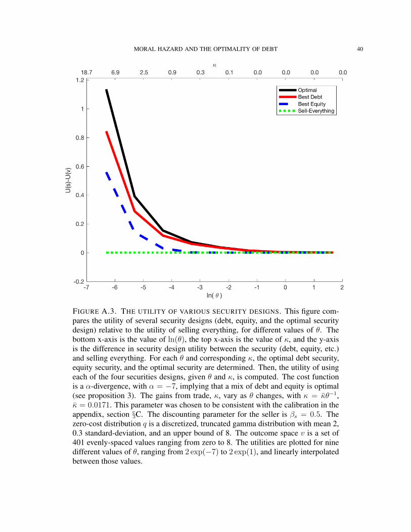
MORAL HAZARD AND THE OPTIMALITY OF DEBT 40
FIGURE A.3. THE UTILITY OF VARIOUS SECURITY DESIGNS. This figure com-pares the utility of several security designs (debt, equity, and the optimal securitydesign) relative to the utility of selling everything, for different values of θ. Thebottom x-axis is the value of ln(θ), the top x-axis is the value of κ, and the y-axisis the difference in security design utility between the security (debt, equity, etc.)and selling everything. For each θ and corresponding κ, the optimal debt security,equity security, and the optimal security are determined. Then, the utility of usingeach of the four securities designs, given θ and κ, is computed. The cost functionis a α-divergence, with α = −7, implying that a mix of debt and equity is optimal(see proposition 3). The gains from trade, κ, vary as θ changes, with κ = κθ−1,κ = 0.0171. This parameter was chosen to be consistent with the calibration in theappendix, section §C. The discounting parameter for the seller is βs = 0.5. Thezero-cost distribution q is a discretized, truncated gamma distribution with mean 2,0.3 standard-deviation, and an upper bound of 8. The outcome space v is a set of401 evenly-spaced values ranging from zero to 8. The utilities are plotted for ninedifferent values of θ, ranging from 2 exp(−7) to 2 exp(1), and linearly interpolatedbetween those values.

MORAL HAZARD AND THE OPTIMALITY OF DEBT 41
APPENDIX B. TIMING CONVENTIONS AND BARGAINING
In this appendix section, I will discuss several possible timing conventions for the sequence ofdecisions by the seller during the first period. In that period, the seller designs the security, sells itto the buyer (assuming the buyer accepts), and takes actions that will create or modify the assetsbacking the security. The timing convention refers to the order in which these three steps occur. Inthe first timing convention, the “shelf registration” convention (using the terminology of DeMarzoand Duffie (1999)), the security is designed before the assets are created, but sold afterward. In thesecond timing convention, the “origination” convention, the security is designed and sold after theassets are created. In the third timing convention, the “principal-agent” convention, the securityis designed and sold before the seller takes her actions. In this last convention, it is natural toassume that the asset exists before the security is designed, but its payoffs are modified by theseller’s actions after the security is traded. For the “principal-agent” timing convention, I will alsodiscuss the effects of Nash-bargaining of the security price, and over both the security design andthe security price. Finally, I point out that a requirement for the seller to raise a certain amount offunds from the buyer, as in standard corporate finance models, would also generate “gains fromtrade,” even if the buyer and seller shared a common discount rate.
There are asset securitization examples for each of these timing conventions. For some assetclasses, such as first-lien mortgages, the security design is standardized, and the “shelf registration”timing convention is appropriate. For more unusual assets, the security design varies deal-by-deal,and the “origination” timing convention is appropriate. In some cases, such as the “Bowie bonds”(securitizations of music royalties), maintaining incentives post-securitization is important, and theprincipal-agent timing convention applies.
TABLE 1. Timing Conventions During the First PeriodPrincipal-Agent Timing(1) Security Designed(2) Security Traded(3) Actions Taken
Origination Timing(1) Actions Taken(2) Security Designed(3) Security Traded
Shelf Registration Timing(1) Security Designed(2) Actions Taken(3) Security Traded
The principal-agent timing convention is the simplest convention to analyze. In any sub-gameperfect equilibrium, the seller takes actions that maximize the value of her retained tranche, becausethe price that she receives for the security has already been set. The buyer anticipates this, formingbeliefs about the distribution of outcomes based on the design of the security. The buyer’s beliefsaffect the price that he is willing to pay for the security, and the seller internalizes this when
MORAL HAZARD AND THE OPTIMALITY OF DEBT 42
designing the security. Multiple equilibria are possible if the seller’s optimal actions for a particularretained tranche are not unique, or if there are multiple security designs that maximize the seller’sutility. The moral hazard, in this timing convention, can occur either because the buyer is unawareof the seller’s actions, or because he can observe those actions but is powerless to enforce anyconsequences based on them.
Under the other two timing conventions, I use equilibrium refinements to argue that the optimalsecurity design and actions associated with the principal-agent timing convention describe the mostappealing equilibria of the game with those alternative timing conventions. I have drawn extensive-form game trees for these two timings in Figure B.1 and Figure B.2 below. The results I presentare related to the findings of Matthews (1995) and Matthews (2001). Matthews (1995) shows, ina closely related model in which contracts are renegotiable, and there is no limited liability, thatall equilibria are “second best efficient,” which is related to my result that the timing is irrelevant.Matthews (2001) extends the results of Matthews (1995) to a model with limited liability, but withonly one choice (effort) for the agent.
I assume that the actions of the seller are not observed by the buyer, ensuring there is stilla moral hazard. I will discuss the benchmark, non-parametric model described in section §2;the set of feasible actions by the seller, M , is the entire probability simplex. I use the notionof proper equilibrium defined by Myerson (1978), and developed for infinite action spaces bySimon and Stinchcombe (1995). I show that, if the principal-agent timing convention has a uniqueequilibrium security design, price, and set of actions taken by the seller, which involve acceptancewith certainty by the buyer, then this security design, price, set of actions, and acceptance withcertainty also characterize all strong proper equilibria22 of the game with the origination and shelfregistration timing conventions, subject to a technical assumption.
22I have not shown that there is a unique strong proper equilibrium– in theory, there could be multiple equilibria withdifferent acceptance strategies by the buyer for security/price combinations that never occur in equilibrium. However,results in the proof of proposition 8 lead me to believe this is not the case.
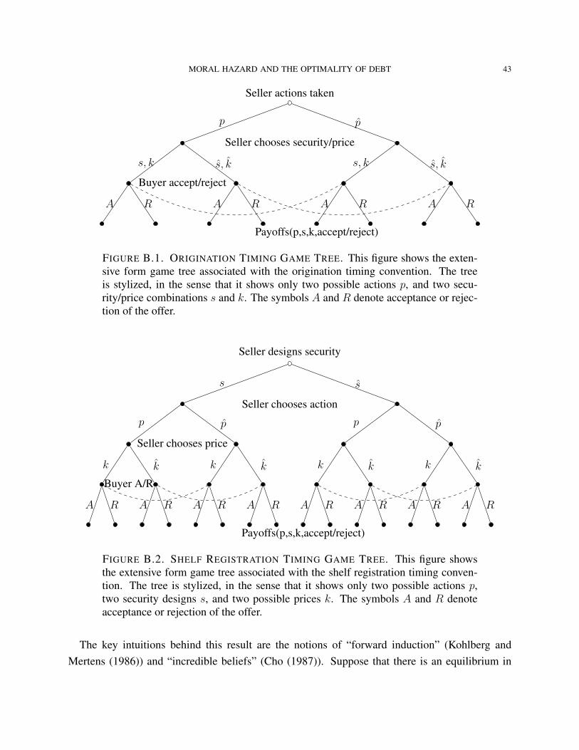
MORAL HAZARD AND THE OPTIMALITY OF DEBT 43
Seller actions taken
A R
s, k
A R
s, k
p
A R
s, k
A R
s, k
p
Seller chooses security/price
Buyer accept/reject
Payoffs(p,s,k,accept/reject)
FIGURE B.1. ORIGINATION TIMING GAME TREE. This figure shows the exten-sive form game tree associated with the origination timing convention. The treeis stylized, in the sense that it shows only two possible actions p, and two secu-rity/price combinations s and k. The symbols A and R denote acceptance or rejec-tion of the offer.
Seller designs security
A R
k
A R
k
p
A R
k
A R
k
p
s
A R
k
A R
k
p
A R
k
A R
k
p
s
Seller chooses action
Seller chooses price
Buyer A/R
Payoffs(p,s,k,accept/reject)
FIGURE B.2. SHELF REGISTRATION TIMING GAME TREE. This figure showsthe extensive form game tree associated with the shelf registration timing conven-tion. The tree is stylized, in the sense that it shows only two possible actions p,two security designs s, and two possible prices k. The symbols A and R denoteacceptance or rejection of the offer.
The key intuitions behind this result are the notions of “forward induction” (Kohlberg andMertens (1986)) and “incredible beliefs” (Cho (1987)). Suppose that there is an equilibrium in

MORAL HAZARD AND THE OPTIMALITY OF DEBT 44
the origination timing in which the buyer is always offered a particular security, s. Now imaginethat the seller plays an off-equilibrium strategy, and offers the buyer a different security, s. Whatshould the buyer believe about the unobservable actions taken by the seller? The notion of forwardinduction recognizes the seller controls both the security design and her actions, and infers fromthe seller’s offer of security s that the seller has taken actions consistent with the buyer acceptingor rejecting that offer. That is, the seller might have taken actions that anticipated a lower or higherprobability of the buyer accepting her offer, but the seller did not take actions that are not bestresponses to some acceptance strategy of the buyer, conditional on having offered the security s tothe buyer. As a result, the buyer should accept or reject the security s based on the belief that theseller has acted in this way, and not rely on “incredible beliefs.” In particular, these notions ruleout the idea that the buyer, when offered security s instead of the security s, can believe the selleris “out to get him,” in the sense that the seller took actions that reduced her own utility in order toharm the buyer.23 These beliefs are not credible; the buyer cannot pretend to hold these beliefs inorder to force the seller to offer him s instead of s.
The notions of forward induction and incredible beliefs, and their associated refinements, are notgenerally equivalent to the proper equilibrium concept. The proper equilibrium concept imposesthe constraint that, in the sequence of mixed strategies whose limit is the equilibrium, actions thatresult in greater utility for the seller must be more likely than actions resulting in lower utilityfor the seller. The buyer’s beliefs, which are governed by Bayes’ rule, must place relatively highweight on the seller playing best-response actions. As a result, in the game I study, proper equilib-rium, forward induction, and restrictions against incredible beliefs end up implementing the sameidea: that, off the equilibrium path, the buyer cannot believe the seller has played an action that isnot a best response, conditional on her observable choice of security design.
The game is structured so that, if the buyer rejects the seller’s take-it-or-leave-it offer, the sellerretains the entire asset (both the security and the retained tranche). For each security design, there isa one-dimensional manifold of best-response actions, each corresponding to a probability that theseller assigns to the buyer’s likelihood of acceptance. The worst case action in this one-dimensionalmanifold, from the perspective increasing the security’s value, is the action that corresponds tothe seller believing the buyer will accept the security with certainty. In that case, the seller hasno incentive to raise the value of the security. The other actions in this one-dimensional manifoldcorrespond to best-responses in which the seller believes she might retain the security, and thereforeacts to increase its value.24
23This argument uses the strategic form of the game, not the agent-strategic form (see Fudenberg and Tirole (1991),chapter 8.4). That is, off-equilibrium security designs are assumed to be correlated with off-equilibrium actions by theseller.24This result depends on the convexity of the set M .

MORAL HAZARD AND THE OPTIMALITY OF DEBT 45
Now consider the optimal security design and price from the principal-agent timing. If the buyeris offered this security design and price, he must be weakly willing to accept, because regardlessof the probabilities he assigns to the seller’s actions over this one-dimensional manifold, the priceis at least fair. The seller, recognizing that the buyer will accept this security and price25, must offerit– it maximizes her utility. This is a heuristic argument that outlines the proof in proposition 8,as it applies to the origination timing. I will now discuss the shelf registration timing, and thendiscuss the technical assumptions required by the proof.
In the shelf registration timing, the security is designed before the actions are taken. As aresult, one might appeal to a notion of sequential rationality to capture the idea that the sellerwould not play non-best-response actions, conditional on the security design that has already beendecided. However, the concept of sequential equilibrium is difficult to extend to games with infiniteaction spaces (see Myerson and Reny (2015)). I will instead use the proper equilibrium concept,recognizing that the results for the shelf registration timing might hold under a weaker equilibriumrefinement.
There is also a significant technical assumption required for the proof of proposition 8. Thetechnicality concerns the compactness of the action spaces available to the agents. The proof ofproposition 8 relies on the proof of existence of strong proper equilibria (theorem 3.1) in Simonand Stinchcombe (1995), which itself requires that the action spaces of the agents be compact.This is problematic, because the buyer’s action space is the set of functions Ab : S ×R→ 0, 1,where S is the set of limited liability securities, 0 represents rejection, and 1 represents acceptanceof the offered security and price. This is not a compact space; the buyer could (in theory) acceptsome particular security and price, while rejecting every offer of the same security with a pricearbitrarily close to the price the buyer would have accepted. The potential for this type of strategyleads Simon and Stinchcombe (1995) to require compact action spaces.
To circumvent these issues, I will require that the seller choose a security and price from a finiteaction space.26 That is, I will define the set S of feasible security designs to be a finite set ofpossible security designs, all of which satisfy the limited liability constraints. I will define the setK to be a finite set of feasible prices.
First, consider the principal-agent timing. Let a(s, k) be the buyer’s acceptance strategy. Thebuyer must accept if the price, k, is less than the buyer’s valuation, βb
∑i>0 p
i(η(s))si, reject if theprice is greater, and is indifferent if the price is equal to the buyer’s valuation. The seller’s payoff,25Actually, some price slightly lower but arbitrarily close to this price.26There are at least three possible alternative strategies. I could have required that the buyer’s strategy satisfy enoughconditions to ensure compactness. Alternatively, I could have pursued the “limit-of-finite” approach described inSimon and Stinchcombe (1995). Finally, I could have attempted to explicitly construct the sequence of mixed strategiesthat generate the proper equilibrium. Each of these seemed to require significant technical work that is beyond thescope of this paper.

MORAL HAZARD AND THE OPTIMALITY OF DEBT 46
given a particular acceptance strategy, is
U(s, k; a) = (1− a(s, k))φ(βsv) + a(s, k)(k + φ(η(s))).
I assume that there is a unique sub-game perfect equilibrium in the principal-agent timing, andthat this equilibrium involves acceptance by the buyer with certainty. Let the s∗ and k∗ denotethe security design and price in this equilibrium, and let p∗ = p(η(s∗)) denote the correspondingoptimal actions. I also assume that the security s∗ is not sell-nothing. I show that, under theseassumptions, all strong proper equilibria of the games with the origination and shelf registrationtiming conventions are also characterized by the security design s∗, the price k∗, the action p∗, andacceptance with certainty.
Proposition 8. In the non-parametric benchmark model described in section §2, if there is a uniquesub-game perfect equilibrium for the game with the principal-agent timing convention, character-ized by security design s∗ ∈ S, price k∗ ∈ K, actions p∗ ∈ M , and acceptance by the buyer,with s∗i > 0 for some i ∈ Ω, then all strong proper equilibrium (in the terminology of Simon andStinchcombe (1995)) of the origination timing and shelf registration timing are characterized bythat security design, price, and action, and the buyer accepting the seller’s offer with certainty.
Proof. See online appendix section 3.18.
The proposition argues that the timing of the game is, in essence, irrelevant. The analysis inthe main body of the paper, regarding when debt contracts are optimal or nearly optimal, appliesregardless of the timing. The proposition, as stated, relies on the strong proper equilibrium con-cept defined by Simon and Stinchcombe (1995), but also applies to those authors’ weak properequilibrium concept.
Next, I will discuss, under the principal-agent timing convention, alternatives to giving all ofthe bargaining power to the seller. I will discuss two alternatives: first, that the seller designs thesecurity, but then Nash-bargains with the buyer over the price, and second, that the seller and buyerbargain jointly over both the security design and price.
First, suppose that the seller and buyer bargain over the price K(η). Let 1− ρ > 0 and ρ > 0 betheir respective bargaining weights. The outside option is no trade: the seller retains everything,and the buyer pays and receives nothing. The price, as a function of the retained tranche (or,equivalently, of the security design), solves
K∗(η) ∈ arg maxK
(βbEp(η)[s(η)]−K)ρ(φ(η) +K − φ(βsv))1−ρ.
Using the first-order conditions to solve for K∗(η),
(B.1) K∗(η) = (1− ρ)βbEp(η)[s] + ρ(φ(βsv)− φ(η)).

MORAL HAZARD AND THE OPTIMALITY OF DEBT 47
The utility in the security design problem is
U(η) = (1− ρ)(βbEp(η)[s(η)] + φ(η)) + ρφ(βsv).
This is simply an affine transformation of the security design utility function described in the text(equation (2.2)), and it follows that the same security design will be optimal. The bargainingpower, in this case, changes only the price at which the agents trade the security. Note also that, ifthe buyer (instead of the seller) designs the security, and then the agents bargain over the price, asimilar result follows.
Now suppose that the agents bargain jointly over the security design and price. The agentsmaximize
U(s∗) = maxK,s∈S
(βbEp(η(s))[s]−K)ρ(φ(η(s)) +K − φ(βsv))1−ρ.
The optimal price, as a function of the optimal security design, is still described by equation (B.1).Substituting this in,
U(s∗) = maxs∈S
(1− ρ)1−ρρρ(βbEp(η(s))[s] + φ(η(s))− φ(βsv)),
which is also an affine transformation of the models described in the main text. It again followsthat, if the agents bargain jointly over both the security design and price, the same security designswould be optimal.
Finally, suppose that the seller and buyer share a common discount rate, β, but that the selleris required to raise a certain amount of funds, I > 0, from the buyer. Using the principal-agenttiming, in the security stage, the seller solves
maxηφ(η)
subject to the limited liability constraints (ηi ∈ [0, βvi]) and the fund raising constraint,
βEp(η)[s(η)] ≥ I.
Let λ ≥ 0 denote the multiplier on the fundraising constraint. For any perturbation η(ε) satisfyingthe limited liability constraints, the first-order condition for the Lagrangian of this problem is
−(λ− 1)∑i∈Ω
pi(η∗)∂ηi∂ε|ε=0+ + λβ
∑i,j∈Ω
s∗j∂pj(η)
∂ηi|η=η∗
∂ηi∂ε|ε=0+ ≤ 0.
If λ = 1 + κ > 1, this expression is identical to equation (2.3), and it follows that the optimalsecurity design in this case will be identical to the case studied in the main text.
MORAL HAZARD AND THE OPTIMALITY OF DEBT 48
I will prove that λ > 1 under the assumption that the solution to the moral hazard problem isalways interior (as in the KL divergence case). Observe that it is always feasible to set
∂ηi∂ε|ε=0+ = s∗i ,
a perturbation that gives some share of the security to the seller instead of the buyer. For thissecurity, we must have λ > 0, as λ = 0 would imply Ep(η)[s(η)] ≤ 0 < I . It follows that theconstraint binds, and therefore
(λ− 1)β−1I ≥ λβ∑i,j∈Ω
s∗j∂pj(η)
∂ηi|η=η∗s
∗i .
Noting that φ(η) is the convex conjugate of ψ(p), and therefore strictly convex, and that ∂pj(η)∂ηi
=
∂i∂jφ(η), the right hand side of the above expression is strictly positive, and therefore λ > 1,completing the proof.
APPENDIX C. CALIBRATION
In this section of the appendix, I will discuss possible calibration strategies for the static, non-parametric model of moral hazard discussed in the main text. I will focus on the context of mort-gage securitization, and how to calibrate the key parameters κ and θ, under the assumption thatthe cost function is the KL divergence, or that the cost function is an invariant divergence and thefirst-order approximation discussed in the text is accurate. In both of these cases, a debt securitydesign is optimal.
In the context of mortgage origination, there is empirical evidence for lax screening by origina-tors who intended to securitize their mortgage loans, which suggests that moral hazard is a rele-vant issue (see Demiroglu and James (2012); Elul (2016); Jiang et al. (2013); Keys et al. (2010);Krainer and Laderman (2014); Mian and Sufi (2009); Nadauld and Sherlund (2013); Purnanandam(2010); Rajan et al. (2015), although some of this evidence is disputed by Bubb and Kaufman(2014)). However, some of this evidence is consistent with information asymmetries but cannotdistinguish between moral hazard and adverse selection. There are also mechanisms to mitigateadverse selection by the seller, such as the inability to retain loans and random selection of loansinto securitization (Keys et al. (2010)).
I will discuss an “experimental” approach to calibration first. This approach is consistent in spiritwith the empirical literature on moral hazard in mortgage lending (Keys et al. (2010); Purnanandam(2010), others). In that literature, the quasi-experiment compares no securitization (ηi = βsvi)with securitization. If we assume securitization uses the optimal security design η∗, then θ can be

MORAL HAZARD AND THE OPTIMALITY OF DEBT 49
approximated (for any invariant divergence cost function, see section §5) as
θ−1 ≈ Ep(βsv)[vi] ·Ep(βsv)[vi]− Ep∗ [vi]
Covp∗(vi, s∗i ).
This formula illustrates the difficulties of calibrating the model using the empirical work onmoral hazard in mortgage lending. For the purposes of the model, what matters is the loss inexpected value due to securitization, relative to the risk taken on by the buyers, ex-ante. Theempirical literature estimates ex-post differences, and the magnitude of these differences variessubstantially, depending on whether the data sample is from before or during the recent crash inhome prices. Converting this into an ex-ante difference would require assigning beliefs to thebuyer and seller about the likelihood of a crash. Estimating the ex-ante covariance, which can beunderstood as a measure of the quantity of “skin in the game,” is even more fraught. For thesereasons, I have not pursed this calibration strategy further.
The second calibration strategy, which is somewhat more promising, is to use the design ofmortgage securities to infer θ. Essentially, by (crudely) estimating the other terms in the “putoption value” equation (equation (3.2)), and assuming the model is correct, we can infer what thesecurity designers thought the moral hazard was. Rearranging that equation,
βbv − βbEp∗ [si]
βbEp∗ [si]︸ ︷︷ ︸Spread
Ep∗ [si]
Ep∗ [vi]︸ ︷︷ ︸Share
(1− Ep(βsv)[vi]− Ep∗ [vi]
Ep(βs(v))[vi]︸ ︷︷ ︸Moral Hazard
)κ−1 = θ.
The spread term should be thought of as reflecting the initial spread between the assets purchasedby the buyer and the discount rate, under the assumption that the bonds will not default. Using a90/10 weighting on the initial AAA and BBB 06-2 ABX coupons reported in Gorton (2008), Iestimate this as 34 basis points per year. In a different setting (CLOs), the work of Nadauld andWeisbach (2012) estimates the cost of capital advantage (gains from trade) due to securitization at17 basis points per year. The “share” term is the ratio of the initial market value of the securityto the initial market value of the assets. Begley and Purnanandam (2016) document that the valueof the non-equity tranches was roughly 99% of the principal value in their sample of residentialmortgage securitizations. Similarly, the moral hazard term is likely to be small. The estimatesof Keys et al. (2010), whose interpretation is disputed by Bubb and Kaufman (2014), imply thatpre-crisis, securitized mortgage loans defaulted at a 3% higher rate27 than loans held in portfolio.Assuming a 50% recovery rate, and using this as an estimate of the ex-ante expected differencein asset value, this suggests that the moral hazard term is roughly 1.5%, and therefore negligiblein this calibration. Combining all of these estimates, I find θ of 2 is consistent with the empirical
27After about one year, ˜11% of securitized loans were in default, compared to ˜8% of loans held in portfolio.

MORAL HAZARD AND THE OPTIMALITY OF DEBT 50
literature on securitization. This calibration assumed that the security design problem with the KLdivergence was being solved. However, this formula also holds (approximately) under invariantdivergences, conditional on the assumption that θ−1 and κ are small enough.
The value of θ = 2 can be compared with the results of Figure A.3. Under the assumptions usedto generate that figure, which are described in its caption, I find that with θ = 2 and κ = 0.85
(17 basis points per year times 5 years), debt would be achieve 99.96% of gains achieved by theoptimal contract, relative to selling everything (and an even larger fraction of the gains relative toselling nothing). Under these parameters, the utility difference between the best debt security andselling nothing would be roughly 0.73% of the total asset value. While that might seem like aneconomically small gain, for a single deal described in Gorton (2008), SAIL 2005-6, the privategains of securitization would be roughly $16.4mm. In contrast, the utility difference between thebest equity security and selling nothing is about 0.56% of the total asset value. The private costof using the optimal equity contract, instead of the optimal debt contract, would be roughly $4mmfor this particular securitization deal.
The numbers discussed in this calculation depend on the assumptions used in Figure A.3, someof which are ad hoc. Nevertheless, they illustrate the general point that it is simultaneously possiblefor debt to be approximately optimal, and for the private gains of securitization to be large.
APPENDIX D. FREE DISPOSAL AND FREE RISK-SHIFTING
In this section, I will discuss the impact that free disposal of output by the seller and free risk-shifting would have on the models discussed in the main. For the static, non-parametric moralhazard problems discussed in sections 3, 4, and 5, the optimal security designs feature monotoneretained tranches. In the proofs, in online appendix lemma 1, I show this is true for any static,non-parametric security design problem with an invariant divergence cost function whose gradient(in p) is continuous in q.
Intuitively, because the optimal retained tranche is monotone even without free disposal, allow-ing for free disposal does not change the optimal security design. To see this formally, I will showthat, with free disposal, it is without loss of generality to consider monotone retained tranches andignore the disposal option. Imagine that there is free disposal. We can write the agent’s moralhazard problem as
φ(η) = supp∈F (r),r∈M
∑i>0
ηipi − ψ(r),
where F (r) is the set of probability distributions first-order stochastically dominated by r, underthe ordering given by Ω. The agent, in effect, makes two choices– first choosing r using thetechnology discussed in the text, then following a (possibly random) output destruction strategy to
MORAL HAZARD AND THE OPTIMALITY OF DEBT 51
create p. The buyer still receives payoff βbEp[s], and therefore the security design utility describedin equation (2.2) is still valid.
Define, for any retained tranche η, the “monotone version”
ηi(η) = maxj∈0,...,i
ηj.
Note that, because vi is weakly increasing in i, such a design does not violate the limited liabilityconstraints. Note also that, because of the monotonicity of ηi(η),∑
i>0
[pi(η)− ri(η)]ηi(η) = 0.
We can rewrite the moral hazard problem as
φ(η) = supp∈F (r),r∈M
∑i>0
(ηi − ηi(η))pi +∑i>0
ηi(η)ri − ψ(r).
It immediately follows that the behavior without output destruction is the same for the two securi-ties: r(η) = r(η(η)).
By the definition of the retained tranche, if ηi < ηj for some i > j, then si > sj . As a result,output destruction hurts the value of the buyer’s security:∑
i>0
[pi(η)− ri(η)]si(η) ≤ 0
for all η. Therefore, utility in in the security design problem is weakly higher under η(η) thanunder η, and it is without loss of generality to consider monotone security designs.
I have shown that free disposal does not affect the static problems discussed in the text– it isequivalent to a restriction to monotone security designs in the absence of free disposal, and theoptimal security designs were monotone even without such a restriction. Conveniently, essentiallythe same proof applies to the dynamic security design problems.
Suppose we modify the stochastic process for the asset value described in section §6 to allowfor output destruction:
dVt = b(Vt, t)dt+ utσ(Vt, t)dt− dYt + σ(Vt, t)dWt,
where dYt ≥ 0 is the seller’s destruction of asset value at time t. To allow such a modification, weneed use as the space of asset values processes the space of RCLL functions on [0, 1], which I willdenote Ω, instead of the space of continuous functions, which I will continue to denote Ω. We alsoneed to allow the security design to be a function on Ω.
I will say that a retained tranche is monotonic in asset value if, for all t ∈ [0, 1], and all V ∈ Ω,η(V ) is weakly increasing in Vt. Using this definition, debt contracts are monotonic in asset value.

MORAL HAZARD AND THE OPTIMALITY OF DEBT 52
It follows immediately that if the seller is given a retained tranche that is monotonic in asset value,she will not destroy asset value. We can define the “monotone version” of the retained tranche inthe following way. Let F (V ) be the set of all RCLL functions on [0, 1] for which, for all f ∈ F (V )
and t ∈ [0, 1],ft ≤ Vt.
The monotone version of η(V ) is
η(η, V ) = supf∈F (V )
η(f).
Note that, because f1 ≤ V1, this retained tranche satisfies the limited liability constraints.The “weak formulation” approach, based on Girsanov’s theorem and described in proposition 5,
can be applied. We can defined an alternative probability space, with measure Q, on which
dXt = b(Xt, t)dt− dYt + σ(Xt, t)dBt,
and a measure P , absolutely continuous with respect to Q, such that, under P , X has the same lawas V under measure P .
Suppose that the retained tranche is not monotonic in asset value. There is some t and someX such that, if the seller reaches state (t,Xt), she will wish to destroy output. If such a state isnever reached with positive probability under measure P (η) (and hence Q), the retained trancheand its monotone version achieve the same utility in the security design problem, holding themeasure P (η) constant. Such a state can never be reached under any measure that is absolutelycontinuous with respect to Q, and therefore the monotone version of the retained tranche will notaffect the agent’s choice of P . It follows, in this case, that it is without loss of generality to assumemonotonicity.
Assume, going forward, that if a non-monotonicity exists, it is reached with positive probability.I will show that, for any retained tranche that induces the seller to destroy some asset value, thereis another retained tranche that does not induce the seller to destroy asset value and achieves higherutility in the security design problem. As a result, the optimal security design is monotone.
Define a modified version of the retained tranche in the following way: for each B ∈ Ω, letXY (η,B) ∈ Ω denote the asset value path that occurs under the seller’s optimal output destructionplan, given retained tranche η and brownian motion B, and let X(B) be the asset value path thatwould occur in the absence of output destruction. Note that X(B) is not affected by the design ofthe retained tranche, and that there is a one-to-one mapping between X and B. We can defined amodified version of the retained tranche, for X ∈ Ω, as
η(X, η) = η(XY (η,B(X))),

MORAL HAZARD AND THE OPTIMALITY OF DEBT 53
where B(X) is the Brownian motion that induces X in the absence of asset value destruction. Fordiscontinuous X , let η(X, η) = 0. Note that, because asset value destruction decreases X1, thismodified retained tranche satisfies the limited liability constraints.
By revealed preference, η(X) does not induce output destruction– if it did, the seller’s outputdestruction given η would not have been optimal. Moreover, η must also induce the same choiceof P ; again, if some different choice of P was preferable, it would also be preferable under thecontract η. It follows that the seller receives the same utility from η and η.
The buyer, however, receives weakly higher utility from η. By the assumptions discussed insection §6, for any realization of the Brownian motion ω ∈ Ω, destruction of output at time tlowers the value of the asset for all times s ≥ t, relative to the asset values that would have beengenerated in the absence of destruction. Et[V1] is always decreased by destruction (by assumption),and s(X) = X1 − β−1
s η(X). As a result, η delivers weakly higher utility than η, and it is withoutloss of generality to study monotone security designs and assume no output destruction.
Finally, I will discuss “free risk-shifting.” As discussed in the text, the strict convexity assump-tion on the divergences I study rules out risk-shifting that is completely free. One implication offree risk-shifting is that there is not necessarily a unique optimal probability distribution for theseller to choose in the moral hazard problem. For the purposes of discussion, suppose that there issome convention by which a single p(η) is determined for each η.
The utility of any security design can be decomposed (along the lines of lemma 1), with freerisk-shifting,as
U(η) = βb∑i∈Ω
qivi − κ∑i∈Ω
pi(η)[ηi − γ(η)βsvi]+
βbβse(η)− c(e(η))− κ
∑i∈Ω
pi(γ(η)βsv)γ(η)βsvi,
where M(e) ⊂M is the set of probability distributions associated with effort level e and
c(e) = minp∈M(e)
ψ(p).
The moral hazard problem can be written as
φ(η) = maxe,p∈M(e)
∑i∈Ω
pi[ηi − γ(η)βsvi]
+∑i∈Ω
pie(e)γ(η)βsvi − c(e),
wherepe(e) = arg min
p∈M(e)ψ(p).

MORAL HAZARD AND THE OPTIMALITY OF DEBT 54
By the seller’s optimal choice of p in the moral hazard problem, it must be the case that∑i∈Ω
pi(η)[ηi − γ(η)βsvi] ≥ 0.
It follows immediately that the equivalent equity tranche delivers higher utility in the securitydesign problem, if it is feasible. If γ(η) > 1, then
U(η) ≤ (1 + κ)βs∑i∈Ω
qivi + (1 + κ)e(η)
− c(e(η))− κ(e+ βs∑i∈Ω
qivi)
≤ βs∑i∈Ω
qivi + e(η)− c(e(η))
≤ βs∑i∈Ω
qivi + e(βsv)− c(e(βsv)),
implying that ηi = βsvi is preferable, and hence γ(η) > 1 is never optimal. Negative effort is alsosub-optimal, and hence the optimal design features γ(η) ∈ [0, 1], and therefore that the equivalentequity tranche is feasible. It follows that, with free risk-shifting, an equity security is always anoptimal security design.
APPENDIX E. APPENDIX REFERENCES
Taylor A. Begley and Amiyatosh K. Purnanandam. Design of financial securities: Empirical evi-dence from private-label rmbs deals. The Review of Financial Studies, 30(1):120–161, 2016.
R. Bubb and A. Kaufman. Securitization and moral hazard: Evidence from credit score cutoffrules. Journal of Monetary Economics, 63:1–18, 2014.
I. K. Cho. A refinement of sequential equilibrium. Econometrica: Journal of the EconometricSociety, pages 1367–1389, 1987.
P. DeMarzo and D. Duffie. A liquidity-based model of security design. Econometrica, 67(1):65–99, 1999.
C. Demiroglu and C. James. How important is having skin in the game? originator-sponsor affilia-tion and losses on mortgage-backed securities. Review of Financial Studies, 25(11):3217–3258,2012.
R. Elul. Securitization and mortgage default. Journal of Financial Services Research, 49(2-3):281–309, 2016.
D. Fudenberg and J. Tirole. Game theory. 1991.G. Gorton. The panic of 2007. Technical report, National Bureau of Economic Research, 2008.

MORAL HAZARD AND THE OPTIMALITY OF DEBT 55
R.D. Innes. Limited liability and incentive contracting with ex-ante action choices. Journal ofEconomic Theory, 52(1):45–67, 1990.
W. Jiang, A. A. Nelson, and E. Vytlacil. Securitization and loan performance: Ex ante and ex postrelations in the mortgage market. Review of Financial Studies, 27(2):454–483, 2013.
B.J. Keys, T. Mukherjee, A. Seru, and V. Vig. Did securitization lead to lax screening? evidencefrom subprime loans. The Quarterly Journal of Economics, 125(1):307–362, 2010.
E. Kohlberg and J. F. Mertens. On the strategic stability of equilibria. Econometrica: Journal ofthe Econometric Society, pages 1003–1037, 1986.
J. Krainer and E. Laderman. Mortgage loan securitization and relative loan performance. Journalof Financial Services Research, 45(1):39–66, 2014.
Steven A Matthews. Renegotiation of sales contracts. Econometrica: Journal of the EconometricSociety, pages 567–589, 1995.
Steven A Matthews. Renegotiating moral hazard contracts under limited liability and monotonicity.Journal of Economic Theory, 97(1):1–29, 2001.
Atif Mian and Amir Sufi. The consequences of mortgage credit expansion: Evidence from the usmortgage default crisis. The Quarterly Journal of Economics, 124(4):1449–1496, 2009.
R. B. Myerson. Refinements of the nash equilibrium concept. International journal of gametheory, 7(2):73–80, 1978.
R. B. Myerson and P. J. Reny. Sequential equilibria of multi-stage games with infinite sets of typesand actions. manuscript, University of Chicago, 2015.
T. D. Nadauld and S. M. Sherlund. The impact of securitization on the expansion of subprimecredit. Journal of Financial Economics, 107(2):454–476, 2013.
T. D. Nadauld and M. S. Weisbach. Did securitization affect the cost of corporate debt? Journalof Financial Economics, 105(2):332–352, 2012.
A. Purnanandam. Originate-to-distribute model and the subprime mortgage crisis. Review ofFinancial Studies, 24(6):1881–1915, 2010.
U. Rajan, A. Seru, and V. Vig. The failure of models that predict failure: distance, incentives anddefaults. Journal of Financial Economics, 115(2):237–260, 2015.
L. K. Simon and M. B. Stinchcombe. Equilibrium refinement for infinite normal-form games.Econometrica: Journal of the Econometric Society, pages 1421–1443, 1995.