introduction to inverse problems the optimality criterion ... to inverse problems the optimality...
TRANSCRIPT

Introduction to inverse problemsThe optimality criterion
Results and examplesConclusion
Optimal design for inverse problems
Stefanie BiedermannSchool of Mathematics and Statistical Sciences Research Institute
University of Southampton, UK
Joint work withNicolai Bissantz, Holger Dette (both Ruhr-Universitat Bochum)
and Edmund Jones (University of Bristol)
Workshop: Experiments for Processes With Time or SpaceDynamics
Isaac Newton Institute, Cambridge, 20 July 2011
Stefanie Biedermann Optimal design for inverse problems

Introduction to inverse problemsThe optimality criterion
Results and examplesConclusion
1 Introduction to inverse problemsWhat is an inverse problem?The modelEstimation
2 The optimality criterion
3 Results and examplesOptimal designsExample in one dimensionSome examples in two dimensions
4 Conclusion
Stefanie Biedermann Optimal design for inverse problems

Introduction to inverse problemsThe optimality criterion
Results and examplesConclusion
What is an inverse problem?The modelEstimation
Example of an inverse problem
Stefanie Biedermann Optimal design for inverse problems

Introduction to inverse problemsThe optimality criterion
Results and examplesConclusion
What is an inverse problem?The modelEstimation
Example of an inverse problem
Stefanie Biedermann Optimal design for inverse problems

Introduction to inverse problemsThe optimality criterion
Results and examplesConclusion
What is an inverse problem?The modelEstimation
Example of an inverse problem
Stefanie Biedermann Optimal design for inverse problems
Introduction to inverse problemsThe optimality criterion
Results and examplesConclusion
What is an inverse problem?The modelEstimation
Example of an inverse problem
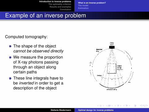
Computed tomography:
The shape of the objectcannot be observed directlyWe measure the proportionof X-ray photons passingthrough an object alongcertain pathsThese line integrals have tobe inverted in order to get adescription of the object
Stefanie Biedermann Optimal design for inverse problems
Introduction to inverse problemsThe optimality criterion
Results and examplesConclusion
What is an inverse problem?The modelEstimation
Applications
Inverse problems occur in many different areas, e.g.
Medical imagingComputed tomographyMagnetic resonance imagingUltrasound
Materials’ Science – find cracks in objects using computedtomography
Geophysics – Borehole tomography
Astrophysics – Imaging of galaxies
All these applications have in common that the feature of interestcannot be observed directly.
Stefanie Biedermann Optimal design for inverse problems
Introduction to inverse problemsThe optimality criterion
Results and examplesConclusion
What is an inverse problem?The modelEstimation
The model - random design
The observations are independent pairs (Xi ,Yi ), i = 1, . . . ,n, where
E[Yi |Xi = x ] = (Km)(x) and Var(Yi |Xi = x) = σ2(x).
m(x) is the object of interest – requires estimationK : L2(µ1)→ L2(µ2) is a compact and injective linear operatorbetween L2-spaces with respect to the probability measures µ1and µ2
X1, . . . ,Xn are the design points drawn randomly from a density hσ2(x) is a positive and finite variance function
Stefanie Biedermann Optimal design for inverse problems
Introduction to inverse problemsThe optimality criterion
Results and examplesConclusion
What is an inverse problem?The modelEstimation
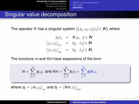
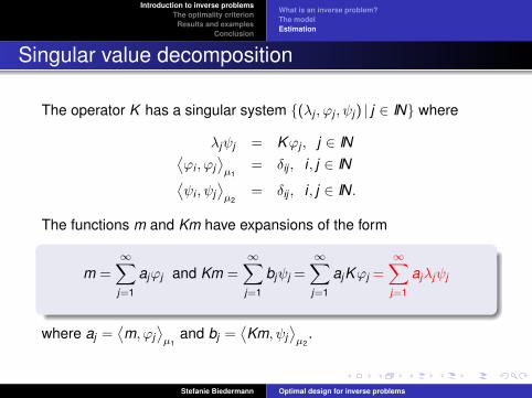
Singular value decomposition
The operator K has a singular system {(λj , ϕj , ψj ) | j ∈ IN} where
λjψj = Kϕj , j ∈ IN⟨ϕi , ϕj
⟩µ1
= δij , i , j ∈ IN⟨ψi , ψj
⟩µ2
= δij , i , j ∈ IN.
The functions m and Km have expansions of the form
m =∞∑j=1
ajϕj and Km =∞∑j=1
bjψj =∞∑j=1
ajKϕj =∞∑j=1
ajλjψj
where aj =⟨m, ϕj
⟩µ1
and bj =⟨Km, ψj
⟩µ2
.
Stefanie Biedermann Optimal design for inverse problems
Introduction to inverse problemsThe optimality criterion
Results and examplesConclusion
What is an inverse problem?The modelEstimation
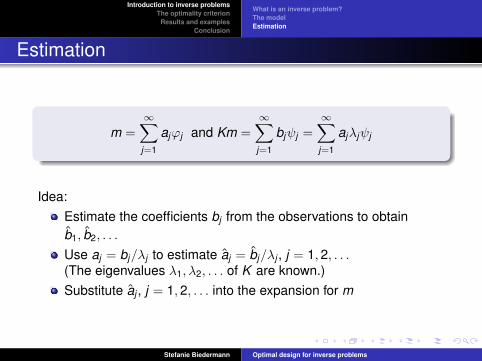
Estimation
m =∞∑j=1
ajϕj and Km =∞∑j=1
bjψj =∞∑j=1
ajλjψj
Idea:Estimate the coefficients bj from the observations to obtainb1, b2, . . .
Use aj = bj/λj to estimate aj = bj/λj , j = 1,2, . . .(The eigenvalues λ1, λ2, . . . of K are known.)Substitute aj , j = 1,2, . . . into the expansion for m
Stefanie Biedermann Optimal design for inverse problems
Introduction to inverse problemsThe optimality criterion
Results and examplesConclusion
What is an inverse problem?The modelEstimation
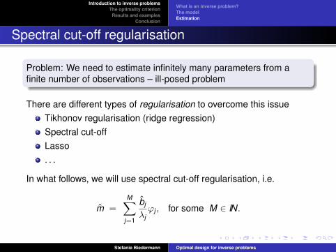
Spectral cut-off regularisation
Problem: We need to estimate infinitely many parameters from afinite number of observations – ill-posed problem
There are different types of regularisation to overcome this issueTikhonov regularisation (ridge regression)Spectral cut-offLasso. . .
In what follows, we will use spectral cut-off regularisation, i.e.
m =M∑
j=1
bj
λjϕj , for some M ∈ IN.
Stefanie Biedermann Optimal design for inverse problems

Introduction to inverse problemsThe optimality criterion
Results and examplesConclusion
The optimality criterion
The goal is to minimise the Integrated Mean Squared Error forestimating m, Φ(h), with respect to the design density h(x).
Φ(h) =1n
∫gM(x)(σ2(x) + (Km)2(x))
h(x)dµ2(x)
+∞∑
j=M+1
b2j
λ2j− 1
n
M∑j=1
b2j
λ2j
where gM(x) =M∑
j=1
ψ2j (x)
λ2j
Note thatOnly the first term of the IMSE depends on hThis term also depends on the unknown functionsσ2(x), (Km)(x) and the unknown regularisation parameter M
Stefanie Biedermann Optimal design for inverse problems
Introduction to inverse problemsThe optimality criterion
Results and examplesConclusion
Optimal designsExample in one dimensionSome examples in two dimensions
The optimal design density
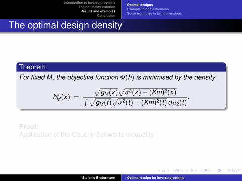
Theorem
For fixed M, the objective function Φ(h) is minimised by the density
h∗M(x) =
√gM(x)
√σ2(x) + (Km)2(x)∫ √
gM(t)√σ2(t) + (Km)2(t) dµ2(t)
.
Proof:Application of the Cauchy-Schwartz inequality
Stefanie Biedermann Optimal design for inverse problems
Introduction to inverse problemsThe optimality criterion
Results and examplesConclusion
Optimal designsExample in one dimensionSome examples in two dimensions
The optimal design density
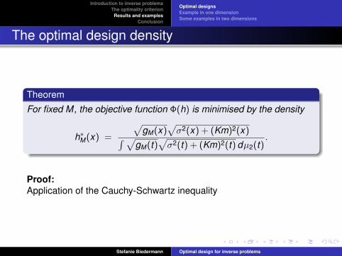
Theorem
For fixed M, the objective function Φ(h) is minimised by the density
h∗M(x) =
√gM(x)
√σ2(x) + (Km)2(x)∫ √
gM(t)√σ2(t) + (Km)2(t) dµ2(t)
.
Proof:Application of the Cauchy-Schwartz inequality
Stefanie Biedermann Optimal design for inverse problems
Introduction to inverse problemsThe optimality criterion
Results and examplesConclusion
Optimal designsExample in one dimensionSome examples in two dimensions
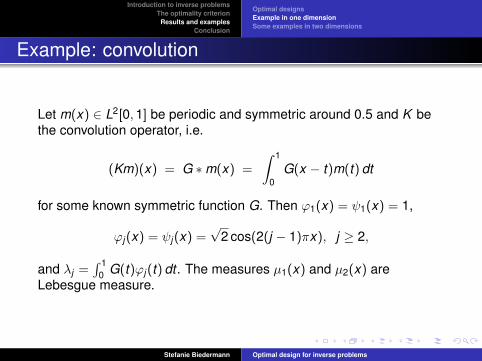
Example: convolution
Let m(x) ∈ L2[0,1] be periodic and symmetric around 0.5 and K bethe convolution operator, i.e.
(Km)(x) = G ∗m(x) =
∫ 1
0G(x − t)m(t) dt
for some known symmetric function G. Then ϕ1(x) = ψ1(x) = 1,
ϕj (x) = ψj (x) =√
2 cos(2(j − 1)πx), j ≥ 2,
and λj =∫ 1
0 G(t)ϕj (t) dt . The measures µ1(x) and µ2(x) areLebesgue measure.
Stefanie Biedermann Optimal design for inverse problems
Introduction to inverse problemsThe optimality criterion
Results and examplesConclusion
Optimal designsExample in one dimensionSome examples in two dimensions
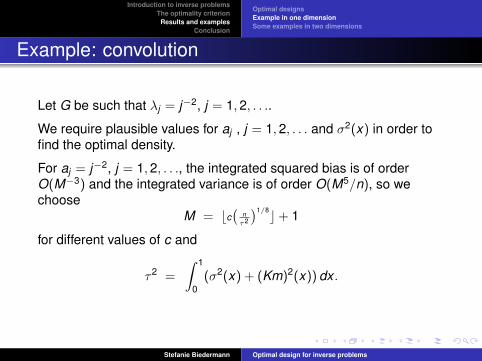
Example: convolution
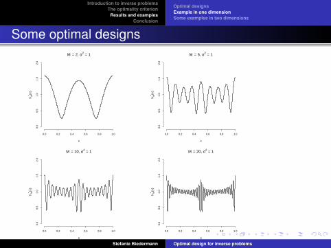
Let G be such that λj = j−2, j = 1,2, . . ..
We require plausible values for aj , j = 1,2, . . . and σ2(x) in order tofind the optimal density.
For aj = j−2, j = 1,2, . . ., the integrated squared bias is of orderO(M−3) and the integrated variance is of order O(M5/n), so wechoose
M = bc(
nτ2
)1/8c+ 1
for different values of c and
τ2 =
∫ 1
0(σ2(x) + (Km)2(x)) dx .
Stefanie Biedermann Optimal design for inverse problems
Introduction to inverse problemsThe optimality criterion
Results and examplesConclusion
Optimal designsExample in one dimensionSome examples in two dimensions
Some optimal designs
0.0 0.2 0.4 0.6 0.8 1.0
0.0
0.5
1.0
1.5
2.0
M = 2, σ2 = 1
x
hM*
(x)
0.0 0.2 0.4 0.6 0.8 1.0
0.0
0.5
1.0
1.5
2.0
M = 5, σ2 = 1
x
hM*
(x)
0.0 0.2 0.4 0.6 0.8 1.0
0.0
0.5
1.0
1.5
2.0
M = 10, σ2 = 1
x
hM*
(x)
0.0 0.2 0.4 0.6 0.8 1.0
0.0
0.5
1.0
1.5
2.0
M = 20, σ2 = 1
x
hM*
(x)
Stefanie Biedermann Optimal design for inverse problems
Introduction to inverse problemsThe optimality criterion
Results and examplesConclusion
Optimal designsExample in one dimensionSome examples in two dimensions
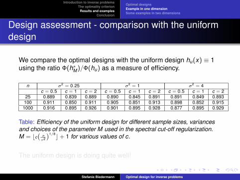
Design assessment - comparison with the uniformdesign
We compare the optimal designs with the uniform design hu(x) ≡ 1using the ratio Φ(h∗M)/Φ(hu) as a measure of efficiency.
n σ2 = 0.25 σ2 = 1 σ2 = 4c = 0.5 c = 1 c = 2 c = 0.5 c = 1 c = 2 c = 0.5 c = 1 c = 2
25 0.889 0.839 0.889 0.890 0.845 0.891 0.891 0.849 0.893100 0.911 0.850 0.911 0.905 0.851 0.913 0.898 0.852 0.915
1000 0.916 0.895 0.926 0.901 0.895 0.928 0.877 0.895 0.929
Table: Efficiency of the uniform design for different sample sizes, variancesand choices of the parameter M used in the spectral cut-off regularization.M = bc
(nτ2
)1/8c+ 1 for various values of c.
The uniform design is doing quite well!
Stefanie Biedermann Optimal design for inverse problems

Introduction to inverse problemsThe optimality criterion
Results and examplesConclusion
Optimal designsExample in one dimensionSome examples in two dimensions
Design assessment - comparison with the uniformdesign
We compare the optimal designs with the uniform design hu(x) ≡ 1using the ratio Φ(h∗M)/Φ(hu) as a measure of efficiency.
n σ2 = 0.25 σ2 = 1 σ2 = 4c = 0.5 c = 1 c = 2 c = 0.5 c = 1 c = 2 c = 0.5 c = 1 c = 2
25 0.889 0.839 0.889 0.890 0.845 0.891 0.891 0.849 0.893100 0.911 0.850 0.911 0.905 0.851 0.913 0.898 0.852 0.915
1000 0.916 0.895 0.926 0.901 0.895 0.928 0.877 0.895 0.929
Table: Efficiency of the uniform design for different sample sizes, variancesand choices of the parameter M used in the spectral cut-off regularization.M = bc
(nτ2
)1/8c+ 1 for various values of c.
The uniform design is doing quite well!
Stefanie Biedermann Optimal design for inverse problems
Introduction to inverse problemsThe optimality criterion
Results and examplesConclusion
Optimal designsExample in one dimensionSome examples in two dimensions
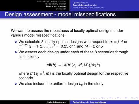
Design assessment - model misspecifications
We want to assess the robustness of locally optimal designs undervarious model misspecifications.
We calculate 8 locally optimal designs with respect to aj = j−2 orj−1.25 (j = 1,2, . . .), σ2 = 0.25 or 1 and M = 2 or 5We assess each design under each of these 8 scenarios throughits efficiency
eff(h) = Φ(h∗(aj , σ2,M))/Φ(h)
where h∗(aj , σ2,M) is the locally optimal design for the respective
scenarioWe also include the uniform design hu in the study
Stefanie Biedermann Optimal design for inverse problems
Introduction to inverse problemsThe optimality criterion
Results and examplesConclusion
Optimal designsExample in one dimensionSome examples in two dimensions
Design assessment - model misspecifications
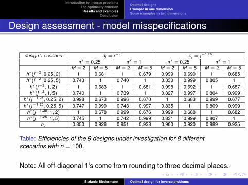
design \ scenario aj = j−2 aj = j−1.25
σ2 = 0.25 σ2 = 1 σ2 = 0.25 σ2 = 1M = 2 M = 5 M = 2 M = 5 M = 2 M = 5 M = 2 M = 5
h∗(j−2, 0.25, 2) 1 0.681 1 0.679 0.999 0.690 1 0.685h∗(j−2, 0.25, 5) 0.743 1 0.740 1 0.830 0.999 0.805 1
h∗(j−2, 1, 2) 1 0.683 1 0.681 0.998 0.692 1 0.687h∗(j−2, 1, 5) 0.740 1 0.739 1 0.827 0.997 0.804 0.999
h∗(j−1.25, 0.25, 2) 0.998 0.673 0.996 0.670 1 0.683 0.999 0.677h∗(j−1.25, 0.25, 5) 0.747 0.999 0.743 0.997 0.835 1 0.809 0.999
h∗(j−1.25, 1, 2) 1 0.678 0.999 0.676 0.999 0.688 1 0.682h∗(j−1.25, 1, 5) 0.745 1 0.742 0.999 0.831 0.999 0.807 1
hu 0.850 0.926 0.851 0.928 0.900 0.920 0.889 0.925
Table: Efficiencies of the 9 designs under investigation for 8 differentscenarios with n = 100.
Note: All off-diagonal 1’s come from rounding to three decimal places.
Stefanie Biedermann Optimal design for inverse problems

Introduction to inverse problemsThe optimality criterion
Results and examplesConclusion
Optimal designsExample in one dimensionSome examples in two dimensions
Design assessment - model misspecifications
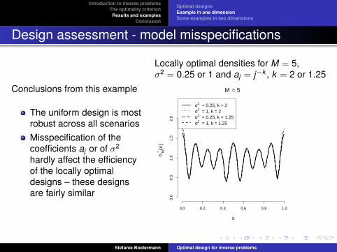
Conclusions from this example
The uniform design is mostrobust across all scenariosMisspecification of thecoefficients aj or of σ2
hardly affect the efficiencyof the locally optimaldesigns – these designsare fairly similar
Stefanie Biedermann Optimal design for inverse problems
Introduction to inverse problemsThe optimality criterion
Results and examplesConclusion
Optimal designsExample in one dimensionSome examples in two dimensions
Design assessment - model misspecifications
Conclusions from this example
The uniform design is mostrobust across all scenariosMisspecification of thecoefficients aj or of σ2
hardly affect the efficiencyof the locally optimaldesigns – these designsare fairly similar
Locally optimal densities for M = 5,σ2 = 0.25 or 1 and aj = j−k , k = 2 or 1.25
0.0 0.2 0.4 0.6 0.8 1.0
0.0
0.5
1.0
1.5
2.0
M = 5
x
hM*
(x)
σ2 = 0.25, k = 2σ2 = 1, k = 2σ2 = 0.25, k = 1.25σ2 = 1, k = 1.25
Stefanie Biedermann Optimal design for inverse problems

Introduction to inverse problemsThe optimality criterion
Results and examplesConclusion
Optimal designsExample in one dimensionSome examples in two dimensions
Radon transform
TomographyWe want to recover thedensity m(r , θ) of an objectfrom line integrals througha sliceEach line or path isparametrised through thedistance s and the angle φThe paths are drawnrandomly from the designdensity h(s, φ)
We observe photon counts→ Poisson distribution
Stefanie Biedermann Optimal design for inverse problems
Introduction to inverse problemsThe optimality criterion
Results and examplesConclusion
Optimal designsExample in one dimensionSome examples in two dimensions
Radon transform
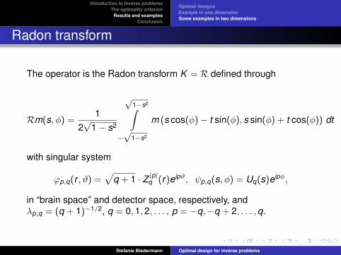
The operator is the Radon transform K = R defined through
Rm(s, φ) =1
2√
1− s2
√1−s2∫
−√
1−s2
m (s cos(φ)− t sin(φ), s sin(φ) + t cos(φ)) dt
with singular system
ϕp,q(r , ϑ) =√
q + 1 · Z |p|q (r)eipϑ, ψp,q(s, φ) = Uq(s)eipφ,
in “brain space” and detector space, respectively, andλp,q = (q + 1)−1/2, q = 0,1,2, . . . , p = −q,−q + 2, . . . ,q.
Stefanie Biedermann Optimal design for inverse problems
Introduction to inverse problemsThe optimality criterion
Results and examplesConclusion
Optimal designsExample in one dimensionSome examples in two dimensions
Radon transform
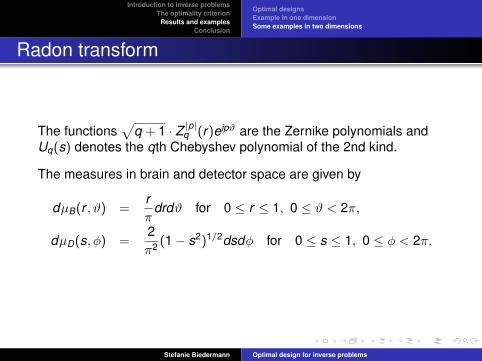
The functions√
q + 1 · Z |p|q (r)eipϑ are the Zernike polynomials andUq(s) denotes the qth Chebyshev polynomial of the 2nd kind.
The measures in brain and detector space are given by
dµB(r , ϑ) =rπ
drdϑ for 0 ≤ r ≤ 1, 0 ≤ ϑ < 2π,
dµD(s, φ) =2π2 (1− s2)1/2dsdφ for 0 ≤ s ≤ 1, 0 ≤ φ < 2π.
Stefanie Biedermann Optimal design for inverse problems
Introduction to inverse problemsThe optimality criterion
Results and examplesConclusion
Optimal designsExample in one dimensionSome examples in two dimensions
The optimal design
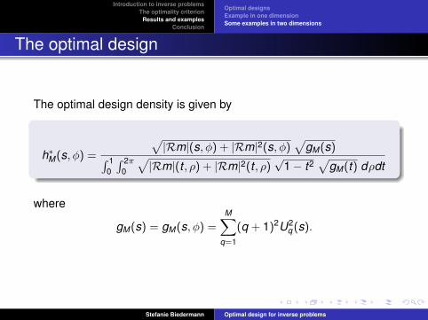
The optimal design density is given by
h∗M(s, φ) =
√|Rm|(s, φ) + |Rm|2(s, φ)
√gM(s)∫ 1
0
∫ 2π0
√|Rm|(t , ρ) + |Rm|2(t , ρ)
√1− t2
√gM(t) dρdt
where
gM(s) = gM(s, φ) =M∑
q=1
(q + 1)2U2q (s).
Stefanie Biedermann Optimal design for inverse problems
Introduction to inverse problemsThe optimality criterion
Results and examplesConclusion
Optimal designsExample in one dimensionSome examples in two dimensions
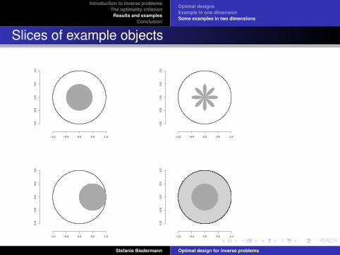
Slices of example objects
−1.0 −0.5 0.0 0.5 1.0
−1.
0−
0.5
0.0
0.5
1.0
−1.0 −0.5 0.0 0.5 1.0
−1.
0−
0.5
0.0
0.5
1.0
−1.0 −0.5 0.0 0.5 1.0
−1.
0−
0.5
0.0
0.5
1.0
−1.0 −0.5 0.0 0.5 1.0
−1.
0−
0.5
0.0
0.5
1.0
Stefanie Biedermann Optimal design for inverse problems

Introduction to inverse problemsThe optimality criterion
Results and examplesConclusion
Optimal designsExample in one dimensionSome examples in two dimensions
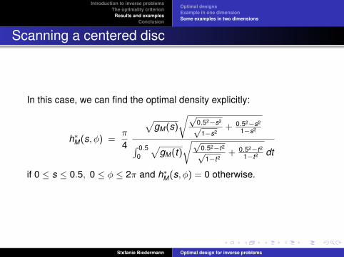
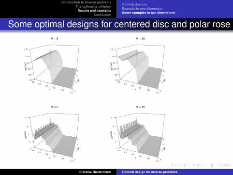
Scanning a centered disc
Suppose we want to scan a solid disc of radius 0.5 positioned in themiddle of the scan field.
−1.0 −0.5 0.0 0.5 1.0
−1.
0−
0.5
0.0
0.5
1.0
Then for each slice,
m(r , θ) =
{1 if 0 ≤ r ≤ 0.50 otherwise.
The Radon transform of this function is given by
Rm(s, φ) =√
0.52 − s2/(√
1− s2)I[0,0.5](s).
Stefanie Biedermann Optimal design for inverse problems
Introduction to inverse problemsThe optimality criterion
Results and examplesConclusion
Optimal designsExample in one dimensionSome examples in two dimensions
Scanning a centered disc
In this case, we can find the optimal density explicitly:
h∗M(s, φ) =π
4
√gM(s)
√√0.52−s2√
1−s2+ 0.52−s2
1−s2∫ 0.50
√gM(t)
√√0.52−t2√
1−t2+ 0.52−t2
1−t2 dt
if 0 ≤ s ≤ 0.5, 0 ≤ φ ≤ 2π and h∗M(s, φ) = 0 otherwise.
Stefanie Biedermann Optimal design for inverse problems

Introduction to inverse problemsThe optimality criterion
Results and examplesConclusion
Optimal designsExample in one dimensionSome examples in two dimensions
Scanning a polar rose
For the polar rose with 8 petals and radius 0.5,
−1.0 −0.5 0.0 0.5 1.0
−1.
0−
0.5
0.0
0.5
1.0
m(r , θ) = 1 if 0 ≤ r ≤ 0.5 | cos(4θ)|, 0 ≤ θ ≤ 2π
and m(r , θ) = 0 otherwise.
Here, the optimal density has to be found numerically.
Stefanie Biedermann Optimal design for inverse problems
Introduction to inverse problemsThe optimality criterion
Results and examplesConclusion
Optimal designsExample in one dimensionSome examples in two dimensions
Some optimal designs for centered disc and polar rose
s
0.00.2
0.40.6
0.81.0
phi
0
2
4
6
h*(s,phi)
0.0
0.5
1.0
1.5
2.0
2.5
.
M = 5
s
0.00.2
0.40.6
0.81.0
phi
0
2
4
6
h*(s,phi)
0.0
0.5
1.0
1.5
2.0
2.5
.
M = 10
s
0.00.2
0.40.6
0.81.0
phi
0
2
4
6
h*(s,phi)
0
1
2
3
4
.
M = 5
s
0.00.2
0.40.6
0.81.0
phi
0
2
4
6
h*(s,phi)
0
1
2
3
4
.
M = 10
Stefanie Biedermann Optimal design for inverse problems

Introduction to inverse problemsThe optimality criterion
Results and examplesConclusion
Optimal designsExample in one dimensionSome examples in two dimensions
Design assessment - comparison with the uniformdesign
n centered disc polar rosec = 0.5 c = 1 c = 2 c = 0.5 c = 1 c = 2
25 .751 (2) .696 (3) .607 (6) .830 (2) .691 (4) .632 (8)100 .833 (3) .658 (5) .611 (9) .910 (3) .725 (6) .646 (11)1000 .915 (4) .733 (8) .620 (15) .950 (5) .842 (9) .679 (18)
10000 .962 (7) .801 (13) .623 (26) .981 (8) .901 (16) .661 (32)
Table: Efficiency of the uniform design on [0, 1]× [0, 2π], in brackets: M.
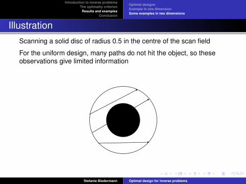
Why is the uniform design doing so poorly this time?
Many observations are made along paths which do not hit the object!
Stefanie Biedermann Optimal design for inverse problems

Introduction to inverse problemsThe optimality criterion
Results and examplesConclusion
Optimal designsExample in one dimensionSome examples in two dimensions
Design assessment - comparison with the uniformdesign
n centered disc polar rosec = 0.5 c = 1 c = 2 c = 0.5 c = 1 c = 2
25 .751 (2) .696 (3) .607 (6) .830 (2) .691 (4) .632 (8)100 .833 (3) .658 (5) .611 (9) .910 (3) .725 (6) .646 (11)1000 .915 (4) .733 (8) .620 (15) .950 (5) .842 (9) .679 (18)
10000 .962 (7) .801 (13) .623 (26) .981 (8) .901 (16) .661 (32)
Table: Efficiency of the uniform design on [0, 1]× [0, 2π], in brackets: M.
Why is the uniform design doing so poorly this time?
Many observations are made along paths which do not hit the object!
Stefanie Biedermann Optimal design for inverse problems
Introduction to inverse problemsThe optimality criterion
Results and examplesConclusion
Optimal designsExample in one dimensionSome examples in two dimensions
IllustrationScanning a solid disc of radius 0.5 in the centre of the scan field
For the uniform design, many paths do not hit the object, so theseobservations give limited information
Stefanie Biedermann Optimal design for inverse problems
Introduction to inverse problemsThe optimality criterion
Results and examplesConclusion
Optimal designsExample in one dimensionSome examples in two dimensions
Design assessment - comparison with the uniformdesign
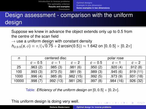
Suppose we knew in advance the object extends only up to 0.5 fromthe centre of the scan field→ use a uniform design with constant densityhU,0.5(s, φ) ≡ π/(
√0.75 + 2 arcsin(0.5)) ≈ 1.642 on [0,0.5]× [0,2π]
n centered disc polar rosec = 0.5 c = 1 c = 2 c = 0.5 c = 1 c = 2
25 .963 (2) .985 (3) .981 (6) .950 (2) .920 (4) .912 (8)100 .993 (3) .973 (5) .981 (9) .989 (3) .945 (6) .919 (11)1000 .996 (4) .985 (8) .982 (15) .992 (5) .973 (9) .931 (18)
10000 .998 (7) .992 (13) .981 (26) .997 (8) .984 (16) .926 (32)
Table: Efficiency of the uniform design on [0, 0.5]× [0, 2π].
This uniform design is doing very well.Stefanie Biedermann Optimal design for inverse problems
Introduction to inverse problemsThe optimality criterion
Results and examplesConclusion
Optimal designsExample in one dimensionSome examples in two dimensions
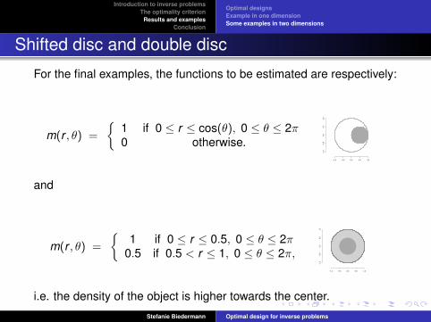
Shifted disc and double disc
For the final examples, the functions to be estimated are respectively:
m(r , θ) =
{1 if 0 ≤ r ≤ cos(θ), 0 ≤ θ ≤ 2π0 otherwise.
−1.0 −0.5 0.0 0.5 1.0
−1.
0−
0.5
0.0
0.5
1.0
and
m(r , θ) =
{1 if 0 ≤ r ≤ 0.5, 0 ≤ θ ≤ 2π
0.5 if 0.5 < r ≤ 1, 0 ≤ θ ≤ 2π,−1.0 −0.5 0.0 0.5 1.0
−1.
0−
0.5
0.0
0.5
1.0
i.e. the density of the object is higher towards the center.
Stefanie Biedermann Optimal design for inverse problems
Introduction to inverse problemsThe optimality criterion
Results and examplesConclusion
Optimal designsExample in one dimensionSome examples in two dimensions
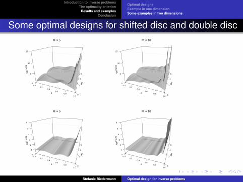
Some optimal designs for shifted disc and double disc
s
0.00.2
0.40.6
0.81.0
phi
0
2
4
6
h*(s,phi)
0
5
10
15
.
M = 5
s
0.00.2
0.40.6
0.81.0
phi
0
2
4
6
h*(s,phi)
0
5
10
15
.
M = 10
s
0.00.2
0.40.6
0.81.0
phi
0
2
4
6
h*(s,phi)
0
1
2
3
4
5
6
.
M = 5
s
0.00.2
0.40.6
0.81.0
phi
0
2
4
6
h*(s,phi)
0
1
2
3
4
5
6
.
M = 10
Stefanie Biedermann Optimal design for inverse problems

Introduction to inverse problemsThe optimality criterion
Results and examplesConclusion
Optimal designsExample in one dimensionSome examples in two dimensions
Design assessment - comparison with the uniformdesign
n shifted disc double discc = 0.5 c = 1 c = 2 c = 0.5 c = 1 c = 2
25 .679 (2) .568 (3) .541 (6) .856 (2) .860 (3) .863 (5)100 .693 (3) .581 (5) .543 (9) .873 (2) .866 (4) .866 (7)1000 .864 (4) .644 (8) .554 (15) .920 (3) .873 (6) .866 (12)
10000 .923 (7) .702 (13) .559 (26) .937 (5) .879 (10) .867 (20)
Table: Efficiency of the uniform design on [0, 1]× [0, 2π].
For the double disc, the uniform design is doing reasonably well. Forthe shifted disc it’s performing quite poorly.
Stefanie Biedermann Optimal design for inverse problems

Introduction to inverse problemsThe optimality criterion
Results and examplesConclusion
Conclusion
The locally optimal designs rarely outperform the uniform designconsiderably . . .
and if they do it can often be remedied using prior knowledge . . .
but not always
The uniform design appears to be more robust with respect tomodel misspecifications
Any prior knowledge on m should be incorporated in the design
Stefanie Biedermann Optimal design for inverse problems

Introduction to inverse problemsThe optimality criterion
Results and examplesConclusion
Future work
Investigate the performance of sequential designs
Consider optimal design for different methods ofmodelling/estimation/regularisation in inverse problems
Consider dynamic problems in this context, e.g. images of abeating heart in real time
Stefanie Biedermann Optimal design for inverse problems

Introduction to inverse problemsThe optimality criterion
Results and examplesConclusion
Thank You!
Stefanie Biedermann Optimal design for inverse problems

Introduction to inverse problemsThe optimality criterion
Results and examplesConclusion
Some references
Biedermann, S.G.M, Bissantz, N., Dette, H. and Jones, E. (2011).Optimal designs for indirect regression. Under review.
Bissantz, N. and Holzmann, H. (2008). Statistical inference for inverseproblems. Inverse problems, 24, 17pp.doi: 10.1088/0266-5611/24/3/034009
Johnstone, I. M. and Silverman, B. W. (1990). Speed of estimation inpositron emission tomography and related inverse problems. Annals ofStatistics, 18, 251-280.
Stefanie Biedermann Optimal design for inverse problems

Introduction to inverse problemsThe optimality criterion
Results and examplesConclusion
Stefanie Biedermann Optimal design for inverse problems
Introduction to inverse problemsThe optimality criterion
Results and examplesConclusion
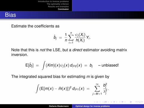
Bias
Estimate the coefficients as
bj =1n
n∑i=1
ψj (Xi )
h(Xi )Yi .
Note that this is not the LSE, but a direct estimator avoiding matrixinversion.
E[bj ] =
∫(Km)(x)ψj (x) dµ2(x) = bj – unbiased!
The integrated squared bias for estimating m is given by∫(E[m(x)− m(x)])2 dµ1(x) =
∞∑j=M+1
b2j
λ2j.
Stefanie Biedermann Optimal design for inverse problems
Introduction to inverse problemsThe optimality criterion
Results and examplesConclusion
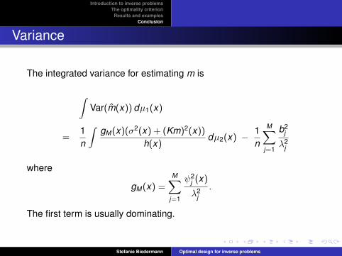
Variance
The integrated variance for estimating m is
∫Var(m(x)) dµ1(x)
=1n
∫gM(x)(σ2(x) + (Km)2(x))
h(x)dµ2(x) − 1
n
M∑j=1
b2j
λ2j
where
gM(x) =M∑
j=1
ψ2j (x)
λ2j.
The first term is usually dominating.
Stefanie Biedermann Optimal design for inverse problems