inverse stieltjes-like functions and inverse problems for systems

Operator Theory:Advances and Applications, Vol. 197, 21–49c© 2009 Birkhauser Verlag Basel/Switzerland

Inverse Stieltjes-like Functionsand Inverse Problems for Systemswith Schrodinger Operator

Sergey Belyi and Eduard Tsekanovskii

To the memory of Moshe Livsic, a remarkable human beingand a great mathematician

Abstract. A class of scalar inverse Stieltjes-like functions is realized as linear-fractional transformations of transfer functions of conservative systems basedon a Schrodinger operator Th in L2[a, +∞) with a non-selfadjoint boundarycondition. In particular it is shown that any inverse Stieltjes function of thisclass can be realized in the unique way so that the main operator A possessesa special semi-boundedness property. We derive formulas that restore thesystem uniquely and allow to find the exact value of a non-real boundaryparameter h of the operator Th as well as a real parameter µ that appearsin the construction of the elements of the realizing system. An elaborateinvestigation of these formulas shows the dynamics of the restored parametersh and µ in terms of the changing free term α from the integral representationof the realizable function.

Mathematics Subject Classification (2000). Primary 47A10, 47B44; Secondary46E20, 46F05.

Keywords. Operator colligation, conservative and impedance system, transfer(characteristic) function.

1. Introduction

The role of realizations of different classes of holomorphic operator-valued func-tions is universally recognized in the spectral analysis of non-self-adjoint operators,interpolation problems, and system theory, with the attention to them growing overthe years. The literature on realization theory is too extensive to be discussed thor-oughly in this paper. We refer a reader, however, to [2], [3], [7], [8], [9], [10], [11],[12], [20], [27], [26], and the literature therein. This paper is the second in a series

22 S.V. Belyi and E.R. Tsekanovskiı

where we study realizations of a subclass of Herglotz-Nevanlinna functions withthe systems based upon a Schrodinger operator. In [14] we have considered a classof scalar Stieltjes-like functions. Here we focus our attention on another impor-tant subclass of Herglotz-Nevanlinna functions, the so-called inverse Stieltjes-likefunctions.

We recall that an operator-valued function V (z) acting on a finite-dimensionalHilbert space E belongs to the class of operator-valued Herglotz-Nevanlinna func-tions if it is holomorphic on C \ R, if it is symmetric with respect to the real axis,i.e., V (z)∗ = V (z), z ∈ C \ R, and if it satisfies the positivity condition

Im V (z) ≥ 0, z ∈ C+.

It is well known (see, e.g., [18], [19]) that operator-valued Herglotz-Nevanlinnafunctions admit the following integral representation:

V (z) = Q + Lz +∫

R

(1

t − z− t

1 + t2

)dG(t), z ∈ C \ R, (1.1)

where Q = Q∗, L ≥ 0, and G(t) is a nondecreasing operator-valued function on R

with values in the class of nonnegative operators in E such that∫R

(dG(t)x, x)E

1 + t2< ∞, x ∈ E. (1.2)

The realization of a selected class of Herglotz-Nevanlinna functions is provided bya linear conservative system Θ of the form{

(A − zI)x = KJϕ−ϕ+ = ϕ− − 2iK∗x (1.3)

or

Θ =(

A K JH+ ⊂ H ⊂ H− E

). (1.4)

In this system A, the main operator of the system, is a so-called (∗)-extension,which is a bounded linear operator from H+ into H− extending a symmetricoperator A in H, where H+ ⊂ H ⊂ H− is a rigged Hilbert space. Moreover, K isa bounded linear operator from the finite-dimensional Hilbert space E into H−,while J = J∗ = J−1 is acting on E, are such that Im A = KJK∗. Also, ϕ− ∈ Eis an input vector, ϕ+ ∈ E is an output vector, and x ∈ H+ is a vector of thestate space of the system Θ. The system described by (1.3)–(1.4) is called a riggedcanonical system of the Livsic type [24] or (in operator theory) the Brodskiı-Livsicrigged operator colligation, cf., e.g., [11], [12], [15]. The operator-valued function

WΘ(z) = I − 2iK∗(A − zI)−1KJ (1.5)

is a transfer function (or characteristic function) of the system Θ. It was shownin [11] that an operator-valued function V (z) acting on a Hilbert space E of theform (1.1) can be represented and realized in the form

V (z) = i[WΘ(z) + I]−1[WΘ(z) − I] = K∗(AR − zI)−1K, (1.6)

Inverse Stieltjes-like Functions and Schrodinger Systems 23

where WΘ(z) is a transfer function of some canonical scattering (J = I) systemΘ, and where the “real part” AR = 1

2 (A + A∗) of A satisfies AR ⊃ A = A∗ ⊃ A ifand only if the function V (z) in (1.1) satisfies the following two conditions:{

L = 0,Qx =

∫R

t1+t2 dG(t)x when

∫R

(dG(t)x, x)E < ∞.(1.7)

In the current paper we specialize in an important subclass of Herglotz-Nevanlinna functions, the class of inverse Stieltjes-like functions that also includesinverse Stieltjes functions (see [13]). In Section 4 we specify a subclass of realizableinverse Stieltjes operator-functions and show that any member of this subclass canbe realized by a system of the form (1.4) whose main operator A satisfies inequality

(ARf, f) ≤ (A∗f, f) + (f, A∗f), f ∈ H+.

In Section 5 we introduce a class of scalar inverse Stieltjes-like functions.Then we rely on the general realization results developed in Section 4 (see also[13] and [14]) to restore a system Θ of the form (1.4) containing the Schrodingeroperator in L2[a, +∞) with non-self-adjoint boundary conditions{

Thy = −y′′ + q(x)yy′(a) = hy(a) ,

(q(x) = q(x), Im h �= 0

).

We show that if a non-decreasing function σ(t) is the spectral distribution functionof a positive self-adjoint boundary value problem{

Aθy = −y′′ + q(x)yy′(a) = θy(a)

and satisfies conditions∞∫

0

dσ(t) = ∞,

∞∫

0

dσ(t)t + t2

< ∞,

then for every real α an inverse Stieltjes-like function

V (z) = α +

∞∫

0

(1

t − z− 1

t

)dσ(t)

can be realized in the unique way as V (z) = VΘ(z) = i[WΘ(z) + I]−1[WΘ(z)− I],where WΘ(z) is the transfer function of a rigged canonical system Θ containingsome Schrodinger operator Th. In particular, it is shown that for every α ≤ 0 aninverse Stieltjes function V (z) with integral representation above can be realizedby a system Θ whose main operator A is a (∗)-extension of a Schrodinger operatorTh and satisfies (2.7).

In addition to the general realization results, Section 5 provides the readerwith formulas that allow to find the exact value of a non-real parameter h in thedefinition of Th of the realizing system Θ. A somewhat similar study is presentedin Section 6 to describe the real parameter µ that appears in the construction ofthe elements of the realizing system. An elaborate investigation of these formulas


shows the dynamics of the restored parameters h and µ in terms of a changingfree term α in the integral representation of V (z) above. It will be shown andgraphically presented that the parametric equations for the restored parameter hrepresent different circles whose centers and radii are completely determined by thefunction V (z). Similarly, the behavior of the restored parameter µ are describedby straight lines.

2. Some preliminaries

For a pair of Hilbert spaces H1, H2 we denote by [H1,H2] the set of all boundedlinear operators from H1 to H2. Let A be a closed, densely defined, symmetricoperator in a Hilbert space H with inner product (f, g), f, g ∈ H. Consider therigged Hilbert space

H+ ⊂ H ⊂ H−,

where H+ = D(A∗) and

(f, g)+ = (f, g) + (A∗f, A∗g), f, g ∈ D(A∗).

Note that identifying the space conjugate to H± with H∓, we get that if A ∈[H+,H−] then A∗ ∈ [H+,H−].

Definition 2.1. An operator A ∈ [H+,H−] is called a self-adjoint bi-extension of asymmetric operator A if A = A∗, A ⊃ A, and the operator

Af = Af, f ∈ D(A) = {f ∈ H+ : Af ∈ H}is self-adjoint in H.

The operator A in the above definition is called a quasi-kernel of a self-adjointbi-extension A (see [30]) .

Definition 2.2. An operator A ∈ [H+,H−] is called a (∗)-extension (or correctbi-extension) of an operator T (with non-empty set ρ(T ) of regular points) if

A ⊃ T ⊃ A, A∗ ⊃ T ∗ ⊃ A

and the operator AR = 12 (A + A∗) is a self-adjoint bi-extension of an operator A.

The existence, description, and analog of von Neumann’s formulas for self-adjoint bi-extensions and (∗)-extensions were discussed in [30] (see also [4], [5],[11]). For instance, if Φ is an isometric operator from the defect subspace Ni ofthe symmetric operator A onto the defect subspace N−i, then the formulas belowestablish a one-to one correspondence between (∗)-extensions of an operator Tand Φ

Af = A∗f + iR(Φ − I)x, A∗f = A∗f + iR(Φ− I)y, (2.1)

where x, y ∈ Ni are uniquely determined from the conditions

f − (Φ + I)x ∈ D(T ), f − (Φ + I)y ∈ D(T ∗)


and R is the Riesz-Berezanskii operator of the triplet H+ ⊂ H ⊂ H− that mapsH+ isometrically onto H− (see [30]). If the symmetric operator A has deficiencyindices (n, n), then formulas (2.1) can be rewritten in the following form

Af = A∗f +n∑

k=1

∆k(f)Vk, A∗f = A∗f +

n∑k=1

δk(f)Vk, (2.2)

where {Vj}n1 ∈ H− is a basis in the subspace R(Φ − I)Ni, and {∆k}n

1 , {δk}n1 , are

bounded linear functionals on H+ with the properties

∆k(f) = 0, ∀f ∈ D(T ), δk(f) = 0, ∀f ∈ D(T ∗). (2.3)

Let H = L2[a, +∞) and l(y) = −y′′+q(x)y where q is a real locally summablefunction. Suppose that the symmetric operator{

Ay = −y′′ + q(x)yy(a) = y′(a) = 0 (2.4)

has deficiency indices (1,1). Let D∗ be the set of functions locally absolutely con-tinuous together with their first derivatives such that l(y) ∈ L2[a, +∞). ConsiderH+ = D(A∗) = D∗ with the scalar product

(y, z)+ =∫ ∞

a

(y(x)z(x) + l(y)l(z)

)dx, y, z ∈ D∗.

LetH+ ⊂ L2[a, +∞) ⊂ H−

be the corresponding triplet of Hilbert spaces. Consider operators{Thy = l(y) = −y′′ + q(x)yhy(a) − y′(a) = 0 ,

{T ∗

hy = l(y) = −y′′ + q(x)yhy(a) − y′(a) = 0

, (2.5)

{Ay = l(y) = −y′′ + q(x)yµy(a) − y′(a) = 0

, Im µ = 0.

It is well known [1] that A = A∗. The following theorem was proved in [6].

Theorem 2.3. The set of all (∗)-extensions of a non-self-adjoint Schrodinger op-erator Th of the form (2.5) in L2[a, +∞) can be represented in the form

Ay = −y′′ + q(x)y − 1µ − h

[y′(a) − hy(a)] [µδ(x − a) + δ′(x − a)],

A∗y = −y′′ + q(x)y − 1

µ − h[y′(a) − hy(a)] [µδ(x − a) + δ′(x − a)].

(2.6)

In addition, the formulas (2.6) establish a one-to-one correspondence between theset of all (∗)-extensions of a Schrodinger operator Th of the form (2.5) and all realnumbers µ ∈ [−∞, +∞].

Definition 2.4. An operator T with the domain D(T ) and ρ(T ) �= ∅ acting on aHilbert space H is called accretive if

Re (Tf, f) ≥ 0, ∀f ∈ D(T ).


Definition 2.5. An accretive operator T is called [22] α-sectorial if there exists avalue of α ∈ (0, π/2) such that

cotα |Im (Tf, f)| ≤ Re (Tf, f), f ∈ D(T ).

An accretive operator is called extremal accretive if it is not α-sectorial forany α ∈ (0, π/2).

Definition 2.6. A (∗)-extensions A in Definition 2.2 is called accumulative if

(ARf, f) ≤ (A∗f, f) + (f, A∗f), f ∈ H+. (2.7)

Consider the symmetric operator A of the form (2.4) with defect indices (1,1),generated by the differential operation l(y) = −y′′ + q(x)y. Let ϕk(x, λ) (k = 1, 2)be the solutions of the following Cauchy problems:

l(ϕ1) = λϕ1

ϕ1(a, λ) = 0ϕ′

1(a, λ) = 1,

l(ϕ2) = λϕ2

ϕ2(a, λ) = −1ϕ′

2(a, λ) = 0.

It is well known [1] that there exists a function m∞(λ) (called the Weyl-Titchmarsh function) for which

ϕ(x, λ) = ϕ2(x, λ) + m∞(λ)ϕ1(x, λ)

belongs to L2[a, +∞).Suppose that the symmetric operator A of the form (2.4) with deficiency

indices (1,1) is nonnegative, i.e., (Af, f) ≥ 0 for all f ∈ D(A)). It was shown in[28] that the Schrodinger operator Th of the form (2.5) is accretive if and only if

Re h ≥ −m∞(−0). (2.8)

For real h such that h ≥ −m∞(−0) we get a description of all nonnegative self-adjoint extensions of an operator A. For h = −m∞(−0) the corresponding operator{

AK y = −y′′ + q(x)yy′(a) + m∞(−0)y(a) = 0 (2.9)

is the Kreın-von Neumann extension of A and for h = +∞ the correspondingoperator {

AF y = −y′′ + q(x)yy(a) = 0 (2.10)

is the Friedrichs extension of A (see [28], [6]).

3. Rigged canonical systems with Schrodinger operator

Let A be (∗)-extension of an operator T , i.e.,

A ⊃ T ⊃ A, A∗ ⊃ T ∗ ⊃ A

where A is a symmetric operator with deficiency indices (n, n) and D(A) = D(T )∩D(T ∗). In what follows we will only consider the case when the symmetric operatorA has dense domain, i.e., D(A) = H.


Definition 3.1. A system of equations{(A − zI)x = KJϕ−ϕ+ = ϕ− − 2iK∗x ,

or an array

Θ =(

A K JH+ ⊂ H ⊂ H− E

)(3.1)

is called a rigged canonical system of the Livsic type if:1) E is a finite-dimensional Hilbert space with scalar product (·, ·)E and the

operator J in this space satisfies the conditions J = J∗ = J−1,2) K ∈ [E,H−], kerK = {0},3) Im A = KJK∗, where K∗ ∈ [H+, E] is the adjoint of K.

In the definition above ϕ− ∈ E stands for an input vector, ϕ+ ∈ E is anoutput vector, and x is a state space vector in H. An operator A is called amain operator of the system Θ, J is a direction operator, and K is a channeloperator. A system Θ of the form (3.1) is called an accretive system [14] if its mainoperator A is accretive and accumulative if its main operator A is accumulative,i.e., satisfies (2.7).

An operator-valued function

WΘ(λ) = I − 2iK∗(A − λI)−1KJ (3.2)

defined on the set ρ(T ) of regular points of an operator T is called the transferfunction (characteristic function) of the system Θ, i.e., ϕ+ = WΘ(λ)ϕ−. It isknown [28], [30] that any (∗)-extension A of an operator T (A∗ ⊃ T ⊃ A), whereA is a symmetric operator with deficiency indices (n, n) (n < ∞), D(A) = D(T )∩D(T ∗), can be included as a main operator of some rigged canonical system withdim E < ∞ and invertible channel operator K.

It was also established [28], [30] that

VΘ(λ) = K∗(Re A − λI)−1K (3.3)

is a Herglotz-Nevanlinna operator-valued function acting on a Hilbert space E,satisfying the following relation for λ ∈ ρ(T ), Im λ �= 0

VΘ(λ) = i[WΘ(λ) − I][WΘ(λ) + I]−1J. (3.4)

Alternatively,WΘ(λ) = (I + iVΘ(λ)J)−1(I − iVΘ(λ)J)

= (I − iVΘ(λ)J)(I + iVΘ(λ)J)−1.(3.5)

Let us recall (see [30], [6]) that a symmetric operator with dense domain D(A)is called prime if there is no reducing, nontrivial invariant subspace on which Ainduces a self-adjoint operator. It was established in [29] that a symmetric operatorA is prime if and only if

c.l.s.λ�=λ

Nλ = H. (3.6)


We call a rigged canonical system of the form (3.1) prime if

c.l.s.λ�=λ, λ∈ρ(T )

Nλ = H.

One easily verifies that if system Θ is prime, then a symmetric operator A of thesystem is prime as well.

The following theorem [6], [14] and corollary [14] establish the connectionbetween two rigged canonical systems with equal transfer functions.

Theorem 3.2. Let Θ1 =(

A1 K1 JH+1 ⊂ H1 ⊂ H−1 E

)and

Θ2 =(

A2 K2 JH+2 ⊂ H2 ⊂ H−2 E

)be two prime rigged canonical systems of the

Livsic type with

A1 ⊃ T1 ⊃ A1, A∗1 ⊃ T ∗

1 ⊃ A1,

A2 ⊃ T2 ⊃ A2, A∗2 ⊃ T ∗

2 ⊃ A2,(3.7)

and such that A1 and A2 have finite and equal defect indices.If

WΘ1(λ) = WΘ2(λ), (3.8)

then there exists an isometric operator U from H1 onto H2 such that U+ = U |H+1

is an isometry1 from H+1 onto H+2, U∗− = U∗

+ is an isometry from H−1 ontoH−2, and

UT1 = T2U, A2 = U−A1U−1+ , U−K1 = K2. (3.9)

Corollary 3.3. Let Θ1 and Θ2 be the two prime systems from the statement ofTheorem 3.2. Then the mapping U described in the conclusion of the theorem isunique.

Now we shall construct a rigged canonical system based on a non-self-adjointSchrodinger operator. One can easily check that the (∗)-extension

Ay = −y′′ + q(x)y − 1µ − h

[y′(a) − hy(a)] [µδ(x − a) + δ′(x − a)], Im h > 0

of the non-self-adjoint Schrodinger operator Th of the form (2.5) satisfies the con-dition

Im A =A − A

∗

2i= (., g)g, (3.10)

where

g =(Im h)

12

|µ − h| [µδ(x − a) + δ′(x − a)] (3.11)

1It was shown in [6] that the operator U+ defined this way is an isometry from H+1 onto H+2.

It is also shown there that the isometric operator U∗ : H+2 → H+1 uniquely defines operatorU− = (U∗)∗ : H−1 → H−2.


and δ(x − a), δ′(x − a) are the delta-function and its derivative at the point a.Moreover,

(y, g) =(Im h)

12

|µ − h| [µy(a) − y′(a)], (3.12)

wherey ∈ H+, g ∈ H−,H+ ⊂ L2(a, +∞) ⊂ H−

and the triplet of Hilbert spaces is as discussed in Theorem 2.3. Let E = C,Kc = cg (c ∈ C). It is clear that

K∗y = (y, g), y ∈ H+ (3.13)

and Im A = KK∗. Therefore, the array

Θ =(

A K 1H+ ⊂ L2[a, +∞) ⊂ H− C

)(3.14)

is a rigged canonical system with the main operator A of the form (2.6), thedirection operator J = 1 and the channel operator K of the form (3.13). Our nextlogical step is finding the transfer function of (3.14). It was shown in [6] that

WΘ(λ) =µ − h

µ − h

m∞(λ) + h

m∞(λ) + h, (3.15)

and

VΘ(λ) =(m∞(λ) + µ) Im h

(µ − Re h)m∞(λ) + µRe h − |h|2 . (3.16)

4. Realization of inverse Stieltjes functions

Let E be a finite-dimensional Hilbert space. The scalar versions of the definitionsbelow can be found in [21]. We recall (see [14], [21]) that an operator-valuedHerglotz-Nevanlinna function V (z) is Stieltjes if it is holomorphic in Ext[0, +∞)and

Im [zV (z)]Im z

≥ 0.

Definition 4.1. We will call an operator-valued Herglotz-Nevanlinna functionV (z) ∈ [E, E] by an inverse Stieltjes if V (z) admits the following integral rep-resentation

V (z) = α + β · z +∫ ∞

0

(1

t − z− 1

t

)dG(t), (4.1)

where α ≤ 0, β ≥ 0, and G(t) is a non-decreasing on [0, +∞) operator-valuedfunction such that ∫ ∞

0

(dG(t)e, e)t + t2

< ∞, ∀e ∈ E.


Alternatively (see [21]) an operator-valued function V (z) is inverse Stieltjesif it is holomorphic in Ext[0, +∞) and V (z) ≤ 0 in (−∞, 0). It is known [21] thata function V (z) �= 0 is an inverse Stieltjes function iff the function −(V (z))−1 isStieltjes.

The following definition was given in [13] and provides the description of allrealizable inverse Stieltjes operator-valued functions.

Definition 4.2. An operator-valued inverse Stieltjes function V (z) ∈ [E, E] is saidto be a member of the class S−1(R) if in the representation (4.1) we have

i) β = 0,

ii) αe =∫ ∞

0

1tdG(t)e = 0,

for all e ∈ E with ∫ ∞

0

(dG(t)e, e)E < ∞. (4.2)

In what follows we will, however, be mostly interested in the following sub-class of S−1(R) that was also introduced in [13].

Definition 4.3. An operator-valued inverse Stieltjes function V (z) ∈ S−1(R) is amember of the class S−1

0 (R) if∫ ∞

0

(dG(t)e, e)E = ∞, (4.3)

for all e ∈ E, e �= 0.

It is not hard to see that S−10 (R) is the analogue of the class N0(R) introduced

in [12] and of the class S0(R) discussed in [14].The following statement [13] is the direct realization theorem for the functions

of the class S−10 (R).

Theorem 4.4. Let Θ be an accumulative system of the form (3.1). Then the opera-tor-function VΘ(z) of the form (3.3), (3.4) belongs to the class S−1

0 (R).

The inverse realization theorem can be stated and proved (see [13]) for theclass S−1

0 (R) as follows.

Theorem 4.5. Let a operator-valued function V (z) belong to the class S−10 (R).

Then V (z) admits a realization by an accumulative prime system Θ of the form(3.1) with J = I.

Proof. It was shown in [13] that any member of the class S−10 (R) is realizable by

an accumulative system Θ of the form (3.1) with J = I. Thus all we actually haveto show is that the model system Θ that was constructed in [13] is prime.

As it was also shown in [11], [12], and [13], the symmetric operator A of themodel system Θ is prime and positive, and hence (3.6) takes place. We are goingto show that in this case the system Θ is also prime, i.e.,

c.l.s.λ�=λ, λ∈ρ(T )

Nλ = H. (4.4)


Consider the operator Uλ0λ = (A − λ0I)(A − λI)−1, where A is an arbitrary self-adjoint extension of A. By a simple check one confirms that Uλ0λNλ0 = Nλ. Toprove (4.4) we assume that there is a function f ∈ H such that

f ⊥ c.l.s.λ�=λ, λ∈ρ(T )

Nλ.

Then (f, Uλ0λg) = 0 for all g ∈ Nλ0 and all λ ∈ ρ(T ). But since the system Θ isaccumulative, it follows that there are regular points of T in the upper and lowerhalf-planes. This leads to a conclusion that the function φ(λ) = (f, Uλ0λg) ≡ 0for all λ �= λ. Combining this with (3.6) we conclude that f = 0 and thus (4.4)holds. �

5. Restoring a non-self-adjoint Schrodinger operator Th

In this section we are going to use the realization technique and results developedfor inverse Stieltjes functions in section 4 to obtain the solution of inverse spectralproblem for Schrodinger operator of the form (2.5) in L2[a, +∞) with non-self-adjoint boundary conditions{

Thy = −y′′ + q(x)yy′(a) = hy(a) ,

(q(x) = q(x), Im h �= 0

). (5.1)

Following the framework of [14] we let H = L2[a, +∞) and l(y) = −y′′+q(x)ywhere q is a real locally summable function. We consider a symmetric operatorwith defect indices (1, 1) {

By = −y′′ + q(x)yy′(a) = y(a) = 0

(5.2)

together with its positive self-adjoint extension of the form{Bθy = −y′′ + q(x)yy′(a) = θy(a)

(5.3)

defined in H = L2[a, +∞). A non-decreasing function σ(λ) defined on [0, +∞)is called the distribution function (see [25]) of an operator pair Bθ, B, where Bθ

of the form (5.3) is a self-adjoint extension of symmetric operator B of the form(5.2), and if the formulas

ϕ(λ) = Uf(x),

f(x) = U−1ϕ(λ),(5.4)

establish one-to-one isometric correspondence U between

Lσ2 [0,+∞) and L2[a,+∞).

Moreover, this correspondence is such that the operator Bθ is unitarily equivalentto the operator

Λσϕ(λ) = λϕ(λ), (ϕ(λ) ∈ Lσ2 [0, +∞)) (5.5)


in Lσ2 [0, +∞) while symmetric operator B in (5.2) is unitarily equivalent to the

symmetric operator

Λ0σϕ(λ) = λϕ(λ), D(Λ0

σ) ={

ϕ(λ) ∈ Lσ2 [0, +∞) :

∫ +∞

0

ϕ(λ)dσ(λ) = 0}

.

(5.6)

Definition 5.1. A scalar Herglotz-Nevanlinna function V (z) is called an inverseStieltjes-like function if it has an integral representation

V (z) = α +∫ ∞

0

(1

t − z− 1

t

)dτ(t),

∫ ∞

0

dτ(t)t + t2

< ∞ (5.7)

similar to (4.1) but with an arbitrary (not necessarily non-positive) constant α.

We are going to introduce a new class of realizable scalar inverse Stieltjes-likefunctions whose structure is similar to that of S−1

0 (R) of Section 4.

Definition 5.2. An inverse Stieltjes-like function V (z) is said to be a member ofthe class SL−1

0 (R) if it admits an integral representation

V (z) = α +∫ ∞

0

(1

t − z− 1

t

)dτ(t), (5.8)

where non-decreasing function τ(t) satisfies the following conditions∫ ∞

0

dτ(t) = ∞,

∫ ∞

0

dτ(t)t + t2

< ∞. (5.9)

Consider the following subclasses of SL−10 (R).

Definition 5.3. A function V (z) ∈ SL−10 (R) belongs to the class SL−1

0 (R, K) if∫ ∞

0

dτ(t)t

= ∞. (5.10)

Definition 5.4. A function V (z) ∈ SL−10 (R) belongs to the class SL−1

01 (R, K) if∫ ∞

0

dτ(t)t

< ∞. (5.11)

The following theorem describes the realization of the class SL−10 (R).

Theorem 5.5. Let V (z) ∈ SL−10 (R). Then it can be realized by a prime system Θ

of the form (3.1).

Proof. We start by applying the general realization theorems from [11] and [13] toa Herglotz-Nevanlinna function V (z) and obtain a rigged canonical system of theLivsic type

ΘΛ =(

Λ Kτ 1Hτ

+ ⊂ Lτ2 [0, +∞) ⊂ Hτ− C

), (5.12)


such that V (z) = VΘΛ(z). Following the steps for construction of the model systemdescribed in [11] and [13], we note that

Λ = ReΛ + iKτ(Kτ )∗

is a correct (∗)-extension of an operator T τ such that Λ ⊃ T τ ⊃ Λ0τ where Λ0

τ isdefined in (5.6). The real part ReΛ is a self-adjoint bi-extension of Λ0

τ that hasa quasi-kernel Λτ of the form (5.5). It was also shown in [13] that the operatorΛ possess the accumulative property (2.7). The operator Kτ in the above system(see [11], [13]) is defined by

Kτc = c · α, (Kτ )∗x = (x, α) c ∈ C, α ∈ Hτ−, x(t) ∈ Hτ

+.

In addition we can observe that the function η(λ) ≡ 1 belongs to Hτ−. To confirm

this we need to show that (x, 1) defines a continuous linear functional for everyx ∈ Hτ

+. It was shown in [11], [12] that

Hτ+ = D(Λ0

τ ) �{

c1

1 + t2

}�{

c2t

1 + t2

}, c1, c2 ∈ C. (5.13)

Consequently, every vector x ∈ Hτ+ has three components x = x1 + x2 + x3

according to the decomposition (5.13) above. Obviously, (x1, 1) and (x2, 1) yieldconvergent integrals while (x3, 1) boils down to

∫ ∞

0

t

1 + t2dτ(t).

The convergence of the latter is guaranteed by the definition of inverse Stieltjes-like function. The state space of the system ΘΛ is Hτ

+ ⊂ Lτ2 [0, +∞) ⊂ Hτ

−, whereHτ

+ = D((Λ0τ )∗).

We can also show that the system ΘΛ is a prime system. In order to do sowe need to show that

c.l.s.λ�=λ, λ∈ρ(T τ )

Nλ = Lτ2 [0, +∞), (5.14)

where Nλ are defect subspaces of the symmetric operator Λ0τ . It is known (see [11],

[13]) that Λ0τ is a non-negative prime operator. Hence we can follow the reasoning

of the proof of theorem 4.5 and only confirm that operator T τ has regular pointsin the upper and lower half-planes. To see this we first note that non-negativeoperator Λ0

τ has no kernel spectrum [1] on the left real half-axis. Then we applyTheorem 1 of [1] (see page 149 of vol. 2 of [1]) that gives the complete descriptionof the spectrum of T τ . This theorem implies that there are regular points of T τ

on the left real half-axis. Since ρ(T τ ) is an open set we confirm the presence ofnon-real regular points of T τ in both half-planes. Thus (5.14) holds and ΘΛ is aprime system.

In order to complete the proof of the theorem we merely set

A = Λ = ReΛ + iKτ (Kτ )∗ and K = Kτ . �


At this point we are ready to state and prove the main realization result ofthis paper.

Theorem 5.6. Let V (z) ∈ SL−10 (R) and the function τ(t) be the distribution func-

tion of an operator pair Bθ of the form (5.2) and B of the form (5.3). Then thereexist unique Schrodinger operator Th (Im h > 0) of the form (5.1), operator A

given by (2.6), operator K as in (3.13), and the rigged canonical system of theLivsic type

Θ =(

A K 1H+ ⊂ L2[a, +∞) ⊂ H− C

), (5.15)

of the form (3.14) so that V (z) is realized by Θ, i.e., V (z) = VΘ(z).

Proof. Since τ(t) is the distribution function of the positive self-adjoint operator,then (see [25]) we can completely restore the operator Bθ of the form (5.3) aswell as a symmetric operator B of the form (5.2). It follows from the definition ofthe distribution function above that there is operator U defined in (5.4) establish-ing one-to-one isometric correspondence between Lτ

2 [0, +∞) and L2[a, +∞) whileproviding for the unitary equivalence between the operator Bθ and operator ofmultiplication by independent variable Λτ of the form (5.5).

Let us consider the system ΘΛ of the form (5.12) constructed in the proofof Theorem 5.5. Applying Theorem 3.2 on unitary equivalence to the isometry Udefined in (5.4) we obtain a triplet of isometric operators U+, U , and U−, where

U+ = U∣∣Hτ

+, U∗

− = U∗+.

This triplet of isometric operators will map the rigged Hilbert space of ΘΛ, thatis Hτ

+ ⊂ Lτ2 [0, +∞) ⊂ Hτ

−, into another rigged Hilbert space H+ ⊂ Lτ2 [a, +∞) ⊂

H−. Moreover, U+ is an isometry from Hτ+ = D(Λ0∗

τ ) onto H+ = D(B∗), andU∗− = U∗

+ is an isometry from Hτ+ onto H−. This is true since the operator U

provides the unitary equivalence between the symmetric operators B and Λ0τ .

Now we construct a system

Θ =(

A K 1H+ ⊂ L2[a, +∞) ⊂ H− C

)

where K = U−Kτ and A = U−ΛU−1+ is a correct (∗)-extension of operator T =

UT τU−1 such that A ⊃ T ⊃ B. The real part ReA contains the quasi-kernel Bθ.This construction of A is unique due to the theorem on the uniqueness of a (∗)-extension for a given quasi-kernel (see [30]). On the other hand, all (∗)-extensionsbased on a pair B, Bθ must take form (2.6) for some values of parameters h and µ.Consequently, our function V (z) is realized by the system Θ of the form (5.15) and

V (z) = VΘΛ(z) = VΘ(z). �

The theorem below gives the criteria for the operator Th of the realizingsystem to be accretive.


Theorem 5.7. Let V (z) ∈ SL−10 (R) satisfy the conditions of Theorem 5.5. Then

the operator Th in the conclusion of the Theorem 5.5 is accretive if and only if

α2 − α

∫ ∞

0

dτ(t)t

+ 1 ≥ 0. (5.16)

The operator Th is φ-sectorial for some φ ∈ (0, π/2) if and only if the inequality(5.16) is strict. In this case the exact value of angle φ can be calculated by theformula

tanφ =

∫∞0

dτ(t)t

α2 − α∫∞0

dτ(t)t + 1

. (5.17)

Proof. It was shown in [29] that for the system Θ in (5.15) described in the previoustheorem the operator Th is accretive if and only if the function

Vh(z) = −i[W−1Θ (−1)WΘ(z) + I]−1[W−1

Θ (−1)WΘ(z) − I]

= −i1 − [(m∞(z) + h)/(m∞(z) + h)][(m∞(−1) + h)/(m∞(−1) + h)]1 + [(m∞(z) + h)/(m∞(z) + h)][(m∞(−1) + h)/(m∞(−1) + h)]

,

(5.18)is holomorphic in Ext[0, +∞) and satisfies the following inequality

1 + Vh(0)Vh(−∞) ≥ 0. (5.19)

Here WΘ(z) is the transfer function of (5.15). It is also shown in [29] that theoperator Th is α-sectorial for some α ∈ (0, π/2) if and only if the inequality (5.19)is strict while the exact value of angle α can be calculated by the formula

cotα =1 + Vh(0)Vh(−∞)|Vh(−∞) − Vh(0)| . (5.20)

According to Theorem 5.5 and equation (3.5)

WΘ(z) = (I − iV (z)J)(I + iV (z)J)−1.

By direct calculations one obtains

WΘ(−1) =1 − i

[α − ∫∞

0dτ(t)t+t2

]

1 + i[α − ∫∞0 dτ(t)

t+t2

] , W−1Θ (−1) =

1 + i[α − ∫∞

0dτ(t)t+t2

]

1 − i[α − ∫∞0 dτ(t)

t+t2

] . (5.21)

Using the following notations

c = α −∫ ∞

0

dτ(t)t + t2

and d = α −∫ ∞

0

dτ(t)t

,

and performing straightforward calculations we obtain

WΘ(−1) =1 − i c

1 + i c, WΘ(−∞) =

1 − i d

1 + i d,

and

Vh(0) =c − α

1 + c αand Vh(−∞) =

c − d

1 + c d. (5.22)


Substituting (5.22) into (5.20) and performing the necessary steps we get

cotφ =1 + α d

α − d=

α2 − α∫∞0

dτ(t)t + 1∫∞

0dτ(t)

t

. (5.23)

Taking into account that α− d > 0 we combine (5.19), (5.20) with (5.23) and thiscompletes the proof of the theorem. �

Below we will derive the formulas for calculation of the boundary parameterh in the restored Schrodinger operator Th of the form (5.1). We consider two majorcases.Case 1. In the first case we assume that

∫∞0

dτ(t)t < ∞. This means that our

function V (z) belongs to the class SL−101 (R, K). In what follows we denote

b =∫ ∞

0

dτ(t)t

and m = m∞(−0).

Suppose that b ≥ 2. Then the quadratic inequality (5.16) implies that for all αsuch that

α ∈(−∞,

b −√b2 − 42

]∪[

b +√

b2 − 42

, +∞)

(5.24)

the restored operator Th is accretive. Clearly, this operator is extremal accretive if

α =b ±√

b2 − 42

.

In particular if b = 2 then α = 1 and the function

V (z) = 1 +∫ ∞

0

(1

t − z− 1

t

)dτ(t)

is realized using an extremal accretive Th.Now suppose that 0 < b < 2. Then for every α ∈ (−∞, +∞) the restored

operator Th will be accretive and φ-sectorial for some φ ∈ (0, π/2). Consider afunction V (z) defined by (5.8). Conducting realizations of V (z) by operators Th

for different values of α ∈ (−∞, +∞) we notice that the operator Th with thelargest angle of sectoriality occurs when

α =b

2, (5.25)

and is found according to the formula

φ = arctanb

1 − b2/4. (5.26)

This follows from the formula (5.17), the fact that α2 − α b + 1 > 0 for all α, andthe formula

α2 − α b + 1 =(

α − b

2

)2

+(

1 − b2

4

).


Now we will focus on the description of the parameter h in the restored operatorTh. It was shown in [6] that the quasi-kernel A of the realizing system Θ fromtheorem 5.5 takes a form{

Ay = −y′′ + qyy′(a) = ηy(a)

, η =µRe h − |h|2

µ − Reh(5.27)

On the other hand, since σ(t) is also the distribution function of the positive self-adjoint operator, we can conclude that A equals to the operator Bθ of the form(5.3). This connection allows us to obtain

θ = η =µRe h − |h|2

µ − Re h. (5.28)

Assuming thath = x + iy

we will use (5.28) to derive the formulas for x and y in terms of γ. First, toeliminate parameter µ, we notice that (3.15) and (3.5) imply

WΘ(λ) =µ − h

µ − h

m∞(λ) + h

m∞(λ) + h=

1 − iV (z)1 + iV (z)

. (5.29)

Passing to the limit in (5.29) when λ → −∞ and taking into account thatV (−∞) = α − b and m∞(−∞) = ∞ (see [14]) we obtain

µ − h

µ − h=

1 − i(α − b)1 + i(α − b)

.

Let us denote

a =1 − i(α − b)1 + i(α − b)

. (5.30)

Solving (5.30) for µ yields

µ =h − ah

1 − a.

Substituting this value into (5.28) after simplification produces

x + iy − a(x − iy)x − (x2 + y2)(1 − a)x + iy − a(x − iy) − x(1 − a)

= θ.

After straightforward calculations targeting to represent numerator and denomi-nator of the last equation in standard form one obtains the following relation

x − (α − b) y = θ. (5.31)

It was shown in [29] that the φ-sectoriality of the operator Th and (5.20) lead to

tanφ =Im h

Reh + m∞(−0)=

y

x + m∞(−0). (5.32)

Combining (5.31) and (5.32) one obtains

x − (α − b)(x tan φ + m∞(−0) tan φ) = θ,


or

x =θ + (α − b)m∞(−0) tan φ

1 − (α − b) tan φ.

But tanφ is also determined by (5.17). Direct substitution of

tanφ =b

1 + α(α − b)

into the above equation yields

x = θ +

[θ + m∞(−0)

]b(α − b)

1 + (α − b)2.

Using the short notation and finalizing calculations we get

h = x + iy, x = θ +(α − b)[θ + m]b

1 + (α − b)2, y =

[θ + m]b1 + (α − b)2

. (5.33)

At this point we can use (5.33) to provide analytical and graphical interpre-tation of the parameter h in the restored operator Th. Let

c = (θ + m)b.

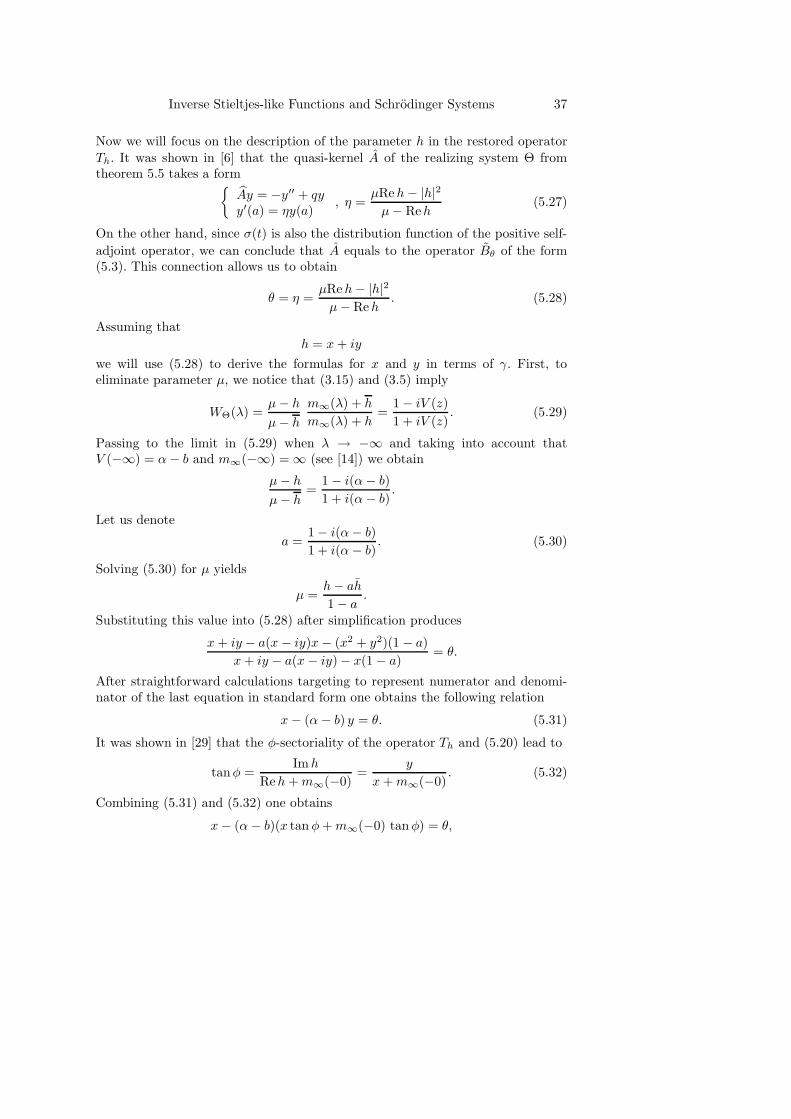
Again we consider three subcases.Subcase 1. b > 2 Using basic algebra we transform (5.33) into

(x − θ)2 +(y − c

2

)2

=c2

4. (5.34)

Since in this case the parameter α belongs to the interval in (5.24), we can seethat h traces the highlighted part of the circle on Figure 1 as α moves from−∞ towards +∞. We also notice that the removed point (θ, 0) correspondsto the value of α = ±∞ while the points h1 and h2 correspond to the valuesα1 = b−√

b2−42 and α2 = b+

√b2−42 , respectively (see Figure 1).

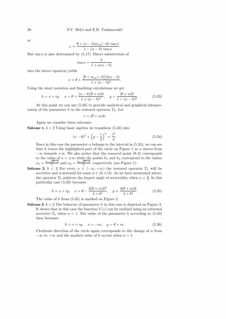
Subcase 2. b < 2 For every α ∈ (−∞, +∞) the restored operator Th will beaccretive and φ-sectorial for some φ ∈ (0, π/2). As we have mentioned above,the operator Th achieves the largest angle of sectoriality when α = b

2 . In thisparticular case (5.33) becomes

h = x + iy, x = θ − 2(θ + m)b2

4 + b2, y =

4(θ + m)b4 + b2

. (5.35)

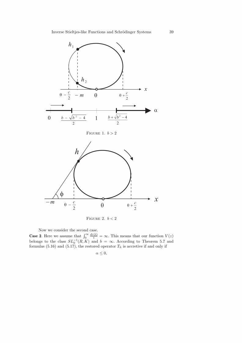
The value of h from (5.35) is marked on Figure 2.Subcase 3. b = 2 The behavior of parameter h in this case is depicted on Figure 3.

It shows that in this case the function V (z) can be realized using an extremalaccretive Th when α = 1. The value of the parameter h according to (5.33)then becomes

h = x + iy, x = −m, y = θ + m. (5.36)

Clockwise direction of the circle again corresponds to the change of α from−∞ to +∞ and the marked value of h occurs when α = 1.


Figure 1. b > 2

Figure 2. b < 2

Now we consider the second case.Case 2. Here we assume that

∫∞0

dτ(t)t = ∞. This means that our function V (z)

belongs to the class SL−10 (R, K) and b = ∞. According to Theorem 5.7 and

formulas (5.16) and (5.17), the restored operator Th is accretive if and only if

α ≤ 0,


Figure 3. b = 2

and φ-sectorial if and only if α < 0. It directly follows from (5.17) that the exactvalue of the angle φ is then found from

tan φ = − 1α

. (5.37)

The latter implies that the restored operator Th is extremal if α = 0. This meansthat a function V (z) ∈ SL−1

0 (R, K) is realized by a system with an extremaloperator Th if and only if

V (z) =∫ ∞

0

(1

t − z− 1

t

)dτ(t). (5.38)

On the other hand since α ≤ 0 the function V (z) is an inverse Stieltjes functionof the class S−1

0 (R). Applying realization theorems from [13] we conclude thatV (z) admits realization by an accumulative system Θ of the form (3.1) with AR

containing the Friedrichs extension AF as a quasi-kernel. Here AF is defined by(2.10). This yields

θ =µx − (x2 + y2)

µ − x= ∞, (5.39)

and hence µ = x. As in the beginning of the previous case we derive the formulasfor x and y, where h = x + iy. Assuming that α �= 0 and using (5.32) and (5.37)leads to

x = µ, y = −x + m

α. (5.40)

To proceed, we first notice that our function V (z) satisfies the conditions ofTheorem 4.9 of [6]. Indeed, the inequality

µ ≥ (Im h)2

m∞(−0) + Re h+ Reh,


that is required to apply this theorem, in our case turns into

µ ≥ − 1α

+ µ,

that is obvious if α < 0. Applying Theorem 4.9 of [6] yields

∞∫

0

dτ(t)1 + t2

=Im h

|µ − h|2

sup

y∈D(AF )

|µy(a) − y′(a)|(∞∫a

(|y(x)|2 + |l(y)|2) dx

) 12

2

. (5.41)

Taking into account that for the case of AF

|µy(a) − y′(a)| = |y′(a)|

and setting

d1/2 = supy∈D(AF )

|y′(a)|(∞∫a

(|y(x)|2 + |l(y)|2) dx

) 12, (5.42)

we obtain

Im h

|µ − h|2 d =

∞∫

0

dτ(t)1 + t2

. (5.43)

Considering that Imh = y and µ = x, solving (5.43) for y yields

y =d∫∞

0dτ(t)1+t2

. (5.44)

Consequently, equations (5.40) describing h = x + iy take form

x = −m +α d∫∞

0dτ(t)1+t2

, y =d∫∞

0dτ(t)1+t2

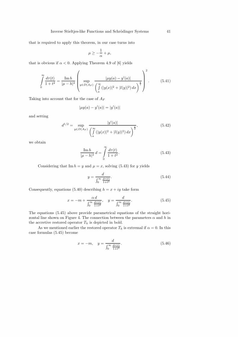
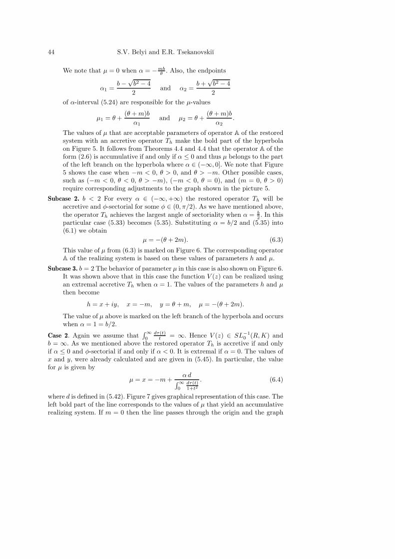
. (5.45)

The equations (5.45) above provide parametrical equations of the straight hori-zontal line shown on Figure 4. The connection between the parameters α and h inthe accretive restored operator Th is depicted in bold.

As we mentioned earlier the restored operator Th is extremal if α = 0. In thiscase formulas (5.45) become

x = −m, y =d∫∞

0dτ(t)1+t2

. (5.46)


Figure 4. b = ∞

6. Realizing systems with Schrodinger operator

Now once we described all the possible outcomes for the restored accretive operatorTh, we can concentrate on the main operator A of the system (5.15). We recallthat A is defined by formulas (2.6) and beside the parameter h above contains alsoparameter µ. We will obtain the behavior of µ in terms of the components of ourfunction V (z) the same way we treated the parameter h. As before we considertwo major cases dividing them into subcases when necessary.

Case 1. Assume that b =∫∞0

dτ(t)t < ∞. In this case our function V (z) belongs to

the class SL−101 (R, K). First we will obtain the representation of µ in terms of x

and y, where h = x + iy. We recall that

µ =h − ah

1 − a,

where a is defined by (5.30). By direct computations we derive that

a =1 − (α − b)2

1 + (α − b)2− 2(α − b)

1 + (α − b)2i, 1 − a =

2(α − b)2

1 + (α − b)2+

2(α − b)1 + (α − b)2

i,

and

h− ah =(

2(α − b)2

1 + (α − b)2x +

2(α − b)1 + (α − b)2

y

)+(

21 + (α − b)2

y +2(α − b)

1 + (α − b)2x

)i.


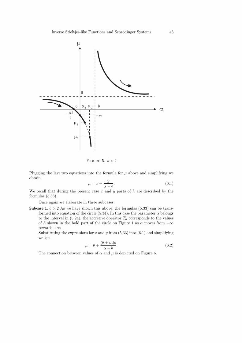
Figure 5. b > 2

Plugging the last two equations into the formula for µ above and simplifying weobtain

µ = x +y

α − b. (6.1)

We recall that during the present case x and y parts of h are described by theformulas (5.33).

Once again we elaborate in three subcases.Subcase 1. b > 2 As we have shown this above, the formulas (5.33) can be trans-

formed into equation of the circle (5.34). In this case the parameter α belongsto the interval in (5.24), the accretive operator Th corresponds to the valuesof h shown in the bold part of the circle on Figure 1 as α moves from −∞towards +∞.Substituting the expressions for x and y from (5.33) into (6.1) and simplifyingwe get

µ = θ +(θ + m)b

α − b. (6.2)

The connection between values of α and µ is depicted on Figure 5.


We note that µ = 0 when α = −mbθ . Also, the endpoints

α1 =b −√

b2 − 42

and α2 =b +

√b2 − 42

of α-interval (5.24) are responsible for the µ-values

µ1 = θ +(θ + m)b

α1and µ2 = θ +

(θ + m)bα2

.

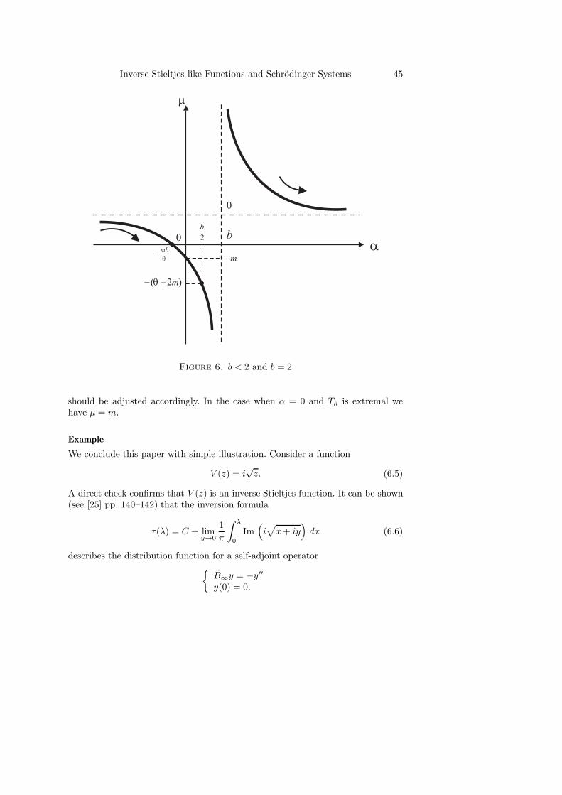
The values of µ that are acceptable parameters of operator A of the restoredsystem with an accretive operator Th make the bold part of the hyperbolaon Figure 5. It follows from Theorems 4.4 and 4.4 that the operator A of theform (2.6) is accumulative if and only if α ≤ 0 and thus µ belongs to the partof the left branch on the hyperbola where α ∈ (−∞, 0]. We note that Figure5 shows the case when −m < 0, θ > 0, and θ > −m. Other possible cases,such as (−m < 0, θ < 0, θ > −m), (−m < 0, θ = 0), and (m = 0, θ > 0)require corresponding adjustments to the graph shown in the picture 5.

Subcase 2. b < 2 For every α ∈ (−∞, +∞) the restored operator Th will beaccretive and φ-sectorial for some φ ∈ (0, π/2). As we have mentioned above,the operator Th achieves the largest angle of sectoriality when α = b

2 . In thisparticular case (5.33) becomes (5.35). Substituting α = b/2 and (5.35) into(6.1) we obtain

µ = −(θ + 2m). (6.3)

This value of µ from (6.3) is marked on Figure 6. The corresponding operatorA of the realizing system is based on these values of parameters h and µ.

Subcase 3. b = 2 The behavior of parameter µ in this case is also shown on Figure 6.It was shown above that in this case the function V (z) can be realized usingan extremal accretive Th when α = 1. The values of the parameters h and µthen become

h = x + iy, x = −m, y = θ + m, µ = −(θ + 2m).

The value of µ above is marked on the left branch of the hyperbola and occurswhen α = 1 = b/2.

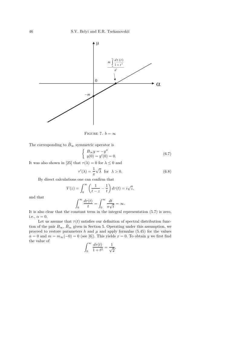
Case 2. Again we assume that∫∞0

dτ(t)t = ∞. Hence V (z) ∈ SL−1

0 (R, K) andb = ∞. As we mentioned above the restored operator Th is accretive if and onlyif α ≤ 0 and φ-sectorial if and only if α < 0. It is extremal if α = 0. The values ofx and y, were already calculated and are given in (5.45). In particular, the valuefor µ is given by

µ = x = −m +α d∫∞

0dτ(t)1+t2

. (6.4)

where d is defined in (5.42). Figure 7 gives graphical representation of this case. Theleft bold part of the line corresponds to the values of µ that yield an accumulativerealizing system. If m = 0 then the line passes through the origin and the graph


Figure 6. b < 2 and b = 2

should be adjusted accordingly. In the case when α = 0 and Th is extremal wehave µ = m.

Example

We conclude this paper with simple illustration. Consider a function

V (z) = i√

z. (6.5)

A direct check confirms that V (z) is an inverse Stieltjes function. It can be shown(see [25] pp. 140–142) that the inversion formula

τ(λ) = C + limy→0

1π

∫ λ

0

Im(i√

x + iy)

dx (6.6)

describes the distribution function for a self-adjoint operator{

B∞y = −y′′

y(0) = 0.


Figure 7. b = ∞

The corresponding to B∞ symmetric operator is{B∞y = −y′′

y(0) = y′(0) = 0.(6.7)

It was also shown in [25] that τ(λ) = 0 for λ ≤ 0 and

τ ′(λ) =1π

√λ for λ > 0. (6.8)

By direct calculations one can confirm that

V (z) =∫ ∞

0

(1

t − z− 1

t

)dτ(t) = i

√z,

and that ∫ ∞

0

dτ(t)t

=∫ ∞

0

dt

π√

t= ∞.

It is also clear that the constant term in the integral representation (5.7) is zero,i.e., α = 0.

Let us assume that τ(t) satisfies our definition of spectral distribution func-tion of the pair B∞, B∞ given in Section 5. Operating under this assumption, weproceed to restore parameters h and µ and apply formulas (5.45) for the valuesα = 0 and m = m∞(−0) = 0 (see [6]). This yields x = 0. To obtain y we first findthe value of ∫ ∞

0

dτ(t)1 + t2

=1√2,


and then use formula (5.42) to get the value of d. This yields d = 1/√

2. Conse-quently,

y =d∫∞

0dτ(t)1+t2

= 1,

and hence h = yi = i. From (6.4) we have that µ = 0 and (2.6) becomes

A y = −y′′ − [iy′(0) + y′(0)]δ′(x). (6.9)

The operator Th in this case is {Thy = −y′′

y′(0) = iy(0).

The channel vector g of the form (3.11) then equals

g = δ′(x), (6.10)

satisfying

Im A =A − A∗

2i= KK∗ = (., g)g,

and channel operator Kc = cg, (c ∈ C) with

K∗y = (y, g) = y′(0). (6.11)

The real part of A

Re A y = −y′′ − y(0)δ′(x)contains the self-adjoint quasi-kernel{

Ay = −y′′

y(0) = 0.

A system of the Livsic type with Schrodinger operator of the form (5.15) thatrealizes V (z) can now be written as

Θ =(

A K 1H+ ⊂ L2[a, +∞) ⊂ H− C

).

where A and K are defined above. Now we can back up our assumption on τ(t) tobe the spectral distribution function of the pair B∞, B∞. Indeed, calculating thefunction VΘ(z) for the system Θ above directly via formula (3.16) with µ = 0 andcomparing the result to V (z) gives the exact value of h = i. Using the uniquenessof the unitary mapping U in the definition of spectral distribution function (seeRemark 5.6 of [14]) we confirm that τ(t) is the spectral distribution function ofthe pair B∞, B∞.

Remark 6.1. All the derivations above can be repeated for an inverse Stieltjes-likefunction

V (z) = α + i√

z, −∞ < α < +∞,

with very minor changes. In this case the restored values for h and µ are describedas follows:

h = x + iy, x = α, y = 1, µ = α.


The dynamics of changing h according to changing α is depicted on Figure 4where the horizontal line has a y-intercept of 1. The behavior of µ is described bya sloped line µ = α (see Figure 7 with m = 0). In the case when α ≤ 0 our functionbecomes inverse Stieltjes and the restored system Θ is accretive. The operators A

and K of the restored system are given according to the formulas (2.6) and (3.13),respectively.

References

[1] N.I. Akhiezer and I.M. Glazman. Theory of linear operators. Pitman Advanced Pub-lishing Program, 1981.

[2] D. Alpay, I. Gohberg, M.A. Kaashoek, A.L. Sakhnovich, “Direct and inverse scat-tering problem for canonical systems with a strictly pseudoexponential potential”,Math. Nachr. 215 (2000), 5–31.

[3] D. Alpay and E.R. Tsekanovskiı, “Interpolation theory in sectorial Stieltjes classesand explicit system solutions”, Lin. Alg. Appl., 314 (2000), 91–136.

[4] Yu.M. Arlinskiı. On regular (∗)-extensions and characteristic matrix-valued functionsof ordinary differential operators. Boundary value problems for differential operators,Kiev, 3–13, 1980.

[5] Yu. Arlinskiı and E. Tsekanovskiı. Regular (∗)-extension of unbounded operators,characteristic operator-functions and realization problems of transfer functions oflinear systems. Preprint, VINITI, Dep.-2867, 72p., 1979.

[6] Yu.M. Arlinskiı and E.R. Tsekanovskiı, “Linear systems with Schrodinger operatorsand their transfer functions”, Oper. Theory Adv. Appl., 149, 2004, 47–77.

[7] D. Arov, H. Dym, “Strongly regular J-inner matrix-valued functions and inverseproblems for canonical systems”, Oper. Theory Adv. Appl., 160, Birkhauser, Basel,(2005), 101–160.

[8] D. Arov, H. Dym, “Direct and inverse problems for differential systems connectedwith Dirac systems and related factorization problems”, Indiana Univ. Math. J. 54(2005), no. 6, 1769–1815.

[9] J.A. Ball and O.J. Staffans, “Conservative state-space realizations of dissipativesystem behaviors”, Integr. Equ. Oper. Theory, 54 (2006), no. 2, 151–213.

[10] H. Bart, I. Gohberg, and M.A. Kaashoek, Minimal Factorizations of Matrix and Op-erator Functions, Operator Theory: Advances and Applications, Vol. 1, Birkhauser,Basel, 1979.

[11] S.V. Belyi and E.R. Tsekanovskiı, “Realization theorems for operator-valued R-functions”, Oper. Theory Adv. Appl., 98 (1997), 55–91.

[12] S.V. Belyi and E.R. Tsekanovskiı, “On classes of realizable operator-valued R-functions”, Oper. Theory Adv. Appl., 115 (2000), 85–112.

[13] S.V. Belyi, S. Hassi, H.S.V. de Snoo, and E.R. Tsekanovskiı, “On the realizationof inverse of Stieltjes functions”, Proceedings of MTNS-2002, University of NotreDame, CD-ROM, 11p., 2002.


[14] S.V. Belyi and E.R. Tsekanovskiı, “Stieltjes-like functions and inverse problems forsystems with Schrodinger operator”, Operators and Matrices., vol. 2, no. 2, (2008),pp. 265–296.

[15] Brodskii, M.S., Triangular and Jordan Representations of Linear Operators, Amer.Math. Soc., Providence, RI, 1971.

[16] M.S. Brodskii, M.S. Livsic. Spectral analysis of non-selfadjoint operators and inter-mediate systems, Uspekhi Matem. Nauk, XIII, no. 1 (79), [1958], 3–84.

[17] V.A. Derkach, M.M. Malamud, and E.R. Tsekanovskiı, Sectorial extensions of a pos-itive operator, and the characteristic function, Sov. Math. Dokl. 37, 106–110 (1988).

[18] F. Gesztesy and E.R. Tsekanovskiı, “On matrix-valued Herglotz functions”, Math.Nachr., 218 (2000), 61–138.

[19] F. Gesztesy, N.J. Kalton, K.A. Makarov, E. Tsekanovskii, “Some Applications ofOperator-Valued Herglotz Functions”, Operator Theory: Advances and Applications,123, Birkhauser, Basel, (2001), 271–321.

[20] S. Khrushchev, “Spectral Singularities of dissipative Schrodinger operator withrapidly decreasing potential”, Indiana Univ. Math. J., 33 no. 4, (1984), 613–638.

[21] I.S. Kac and M.G. Krein, R-functions – analytic functions mapping the upper half-plane into itself, Amer. Math. Soc. Transl. (2) 103, 1–18 (1974).

[22] Kato T.: Perturbation Theory for Linear Operators, Springer-Verlag, 1966

[23] B.M. Levitan, Inverse Sturm-Liouville Problems, VNU Science Press, Utrecht, 1987.

[24] M.S. Livsic, Operators, oscillations, waves, Moscow, Nauka, 1966 (Russian).

[25] M.A. Naimark, Linear Differential Operators II, F. Ungar Publ., New York, 1968.

[26] O.J. Staffans, “Passive and conservative continuous time impedance and scatteringsystems, Part I: Well-posed systems”, Math. Control Signals Systems, 15, (2002),291–315.

[27] O.J. Staffans, Well-posed linear systems, Cambridge University Press, Cambridge,2005.

[28] E.R. Tsekanovskiı, “Accretive extensions and problems on Stieltjes operator-valuedfunctions realizations”, Oper. Theory Adv. Appl., 59 (1992), 328–347.

[29] E.R. Tsekanovskii. “Characteristic function and sectorial boundary value problems”,Investigation on geometry and math. analysis, Novosibirsk, 7, (1987), 180–194.

[30] E.R. Tsekanovskiı and Yu.L. Shmul’yan, “The theory of bi-extensions of operators onrigged Hilbert spaces. Unbounded operator colligations and characteristic functions”,Russ. Math. Surv., 32 (1977), 73–131.

Sergey BelyiDepartment of MathematicsTroy State UniversityTroy, AL 36082, USAe-mail: [email protected]

Eduard TsekanovskiiDepartment of MathematicsNiagara University, NY 14109, USAe-mail: [email protected]

inverse stieltjes-like functions and inverse problems for systems

Documents