universidade de coimbra faculdade de ciˆencias e tecnologia · universidade de coimbra faculdade...
TRANSCRIPT
UNIVERSIDADE DE COIMBRA
Faculdade de Ciencias e Tecnologia
Departamento de Quımica
Accurate ab initio-based doublemany-body expansion potentialenergy surfaces and dynamics for
sulfur-hydrogen molecules
Yu Zhi Song
COIMBRA
2011

UNIVERSIDADE DE COIMBRA
Faculdade de Ciencias e Tecnologia
Departamento de Quımica
Accurate ab initio-based doublemany-body expansion potentialenergy surfaces and dynamics for
sulfur-hydrogen molecules
Dissertation presented for fulfillment
of the requirements for the degree of
“Doutor em Ciencias, especialidade em
Quımica Teorica”
Yu Zhi Song
COIMBRA2011


Dedicated to my family


Acknowledgments
First and foremost, I would like to express my sincere thanks to my supervisor,
Professor Antonio J. C. Varandas, for his inspirational instructions, patient guid-
ance and invaluable encouragement throughout my PhD study at the Department
of Chemistry, University of Coimbra, Portugal. I greatly admire and appreciate
his comprehensive knowledge of Theoretical Chemistry and perseverance attitude
toward scientific research. His effort, knowledge and attitude lead me step by step
to advance in my study, and finally make this dissertation possible.
Besides, I would like to thank all the members of the Theoretical and Com-
putational Chemistry (T&CC) Group. They have created a friendly and warm
atmosphere. Especially, I acknowledge Dr. Sergio P. J. Rodrigues, Dr. Pedro
J. S. B. Caridade and Dr. Luıs A. Poveda for their instructions, discussions
and comments. Much thanks should also be given to all the other members in
our group: Yongqing Li, Vinıcius C. Mota, Luıs P. Viegas, Breno R. L. Galvao,
Maikel B. Furones, Jing Li, Biplab Sarkar, Angel C. G. Fontes, Alexander Alijah,
and Flavia Rolim.
I deeply express my thanks to my MSc supervisor, Professor Chuankui Wang,
for his supervision and guidance during my MSc study at Shandong Normal
University. I take this opportunity to thank Professor Qingtian Meng and Shenglu
Lin. I managed to join the T&CC group with their recommendation. I am also
grateful to Professor Keli Han for his help during my study in Dalian.
I wish to thank the financial support from Fundacao para a Ciencia e a Tec-
nologia, Portugal, with the reference SFRH/BD/28069/2006.
Finally, in particular, I would like to thank my parents, my wife and my
daughter for their unlimited love, understanding, encouragement and countless
support all these years.

Contents
Acknowledgments v
Foreword 1
Bibliography . . . . . . . . . . . . . . . . . . . . . . . . . . . . . . . . 3
I Theoretical framework 7
1 Concept of potential energy surface 9
1.1 Adiabatic representation . . . . . . . . . . . . . . . . . . . . . . . 9
1.2 Born-Oppenheimer approximation . . . . . . . . . . . . . . . . . . 12
1.3 Crossing of adiabatic potentials . . . . . . . . . . . . . . . . . . . 13
1.4 Features of potential energy surface . . . . . . . . . . . . . . . . . 14
Bibliography . . . . . . . . . . . . . . . . . . . . . . . . . . . . . . . . 15
2 Calculation and representation of potential energy surface 17
2.1 Hartree-Fock theory . . . . . . . . . . . . . . . . . . . . . . . . . 17
2.1.1 Derivation of the expectation value . . . . . . . . . . . . . 18
2.1.2 Derivation of the Hartree-Fock equation . . . . . . . . . . 21
2.2 Koopmans’ theorem . . . . . . . . . . . . . . . . . . . . . . . . . . 23
2.3 Configuration interaction method . . . . . . . . . . . . . . . . . . 24
2.4 Multiconfigurational SCF method . . . . . . . . . . . . . . . . . . 26
2.5 Multireference CI method . . . . . . . . . . . . . . . . . . . . . . 27
2.6 Møller-Plesset perturbation theory . . . . . . . . . . . . . . . . . 30
2.7 Coupled cluster theory . . . . . . . . . . . . . . . . . . . . . . . . 31
2.8 Basis sets . . . . . . . . . . . . . . . . . . . . . . . . . . . . . . . 34
viii Contents
2.8.1 Slater and Gaussian type orbitals . . . . . . . . . . . . . . 34
2.8.2 Classification of basis sets . . . . . . . . . . . . . . . . . . 36
2.8.3 Basis set superposition error . . . . . . . . . . . . . . . . . 37
2.9 Semiempirical correction of ab initio energies . . . . . . . . . . . . 38
2.9.1 Scaling the external correlation energy . . . . . . . . . . . 38
2.9.2 Extrapolation to complete basis set limit . . . . . . . . . . 39
2.10 Analytical representation of potential energy surface . . . . . . . . 42
2.10.1 The many-body expansion method . . . . . . . . . . . . . 43
2.10.2 The double many-body expansion method . . . . . . . . . 44
2.10.3 Approximate single-sheeted representation . . . . . . . . . 45
Bibliography . . . . . . . . . . . . . . . . . . . . . . . . . . . . . . . . 47
3 Exploring PESs via dynamics calculations 57
3.1 Quantum dynamics . . . . . . . . . . . . . . . . . . . . . . . . . . 57
3.2 The QCT method . . . . . . . . . . . . . . . . . . . . . . . . . . . 59
3.2.1 Unimolecular decomposition . . . . . . . . . . . . . . . . . 61
3.2.2 Bimolecular reaction . . . . . . . . . . . . . . . . . . . . . 61
3.3 Excitation function and rate constant . . . . . . . . . . . . . . . . 64
3.3.1 Reaction with barrier . . . . . . . . . . . . . . . . . . . . . 64
3.3.2 Barrier-free reaction . . . . . . . . . . . . . . . . . . . . . 65
3.4 Electronic degeneracy factor . . . . . . . . . . . . . . . . . . . . . 66
3.5 Products properties from QCT runs . . . . . . . . . . . . . . . . . 67
3.5.1 Relative velocity and translational energy . . . . . . . . . 68
3.5.2 Velocity scattering angle . . . . . . . . . . . . . . . . . . . 69
3.5.3 Internal energy . . . . . . . . . . . . . . . . . . . . . . . . 69
3.5.4 Rotational angular momentum . . . . . . . . . . . . . . . . 70
3.5.5 Rotational and vibrational energies . . . . . . . . . . . . . 70
Bibliography . . . . . . . . . . . . . . . . . . . . . . . . . . . . . . . . 71
II Case Studies 77
4 CR-CC and MRCI(Q) studies for representative cuts of H2S 79
Contents ix
A comparison of single-reference coupled-cluster and multi-reference
configuration interaction methods for representative cuts of the
H2S(1A′) potential energy surface . . . . . . . . . . . . . . . . . . 81
5 Accurate DMBE/CBS PES for ground-state H2S 105
Accurate ab initio double many-body expansion potential energy surface
for ground-state H2S by extrapolation to the complete basis set limit107
Supporting Information . . . . . . . . . . . . . . . . . . . . . . . . . . 135
6 Accurate DMBE/SEC PES for ground-state H2S 141
Potential energy surface for ground-state H2S via scaling of the external
correlation, comparison with extrapolation to complete basis set
limit, and use in reaction dynamics . . . . . . . . . . . . . . . . . 143
Supporting Information . . . . . . . . . . . . . . . . . . . . . . . . . . 165
7 Accurate DMBE/CBS PES for ground-state HS2 173
Accurate DMBE potential energy surface for ground-state HS2 based
on ab initio data extrapolated to the complete basis set limit . . . 175
Supporting Information . . . . . . . . . . . . . . . . . . . . . . . . . . 205
8 Conclusions and outlook 211
Mathematical appendices 213

Foreword
Atmospheric sulfur chemistry has played a significant role in the early atmosphere
of Earth [1, 2]. In particular, independent isotope fractionation studies are pro-
viding new insight into our understanding of the role that sulfur played in the
early Earth atmosphere [3–6]. Recent studies are also revealing that sulfur chem-
istry is important in the chemical evolution of the atmospheres of giant planets
such as Jupiter [13] and also in the atmosphere of ancient Mars [14]. Reduced
sulfur-containing molecules also show their importance in biochemistry [7–10] and
combustion chemistry [11, 12]. One of the major sulfur-bearing species present
in the atmosphere of the large planets is H2S. The earliest laboratory studies of
the photochemistry of H2S had HS as a major species resulting from the photo-
chemistry [15–17]. Secondary photodissociation of HS radicals has been observed
to produce S atoms [18]. Due to the important role that H2S plays in the various
areas of chemistry, it received much theoretical [19–22] and experimental [23–25]
consideration over the years. Moreover, the HS2 radical plays an important role
in a variety of environments, notably combustion and the oxidation of reduced
forms of sulfur [11, 12, 26, 27]. Amounts of investigation [28–34] have been carried
on HS2 both experimentally and theoretically since Porter [15] first proposed that
the HS2 radical was produced during the photolysis of HSSH. Thus, the model-
ing of accurate global potential energy surfaces (PESs) of H2S and HS2 molecular
systems, combined with dynamics studies, may enhance the understanding of the
atmospheric sulfur chemistry.
The PES of a molecule is a function of the relative positions of the nuclei
whose description is justified within the Born-Oppenheimer [35] separation. An
analytical representation of the PES is achieved using different formalisms, such
as the double many-body expansion (DMBE) method [36–38]. The latter consist
2 Foreword
of expanding the potential energy function of a given molecular system in terms of
the potential energies of its fragments. Information about a PES can be obtained
both from the analysis of experimental data and from ab initio calculations. At
present, robust theoretical frameworks and computational resources make possi-
ble to extensively explore the configuration space with the aim of constructing
accurate and global ab initio-based PESs.
The main goal of the present doctoral thesis is the construction of DMBE
PESs for the electronic ground-state H2S and HS2 molecular system, as well
as the studies of structure, energetics, and spectroscopy. The obtained PESs are
also used for exploratory quasi-classical trajectory calculations of the thermal rate
constants and cross sections of gas-phase reactions. The present PESs for H2S
and HS2 can be employed as building-blocks of DMBE PESs of larger molecular
systems, such as SH3 and H2S2, which contain the mentioned triatoms.
This thesis is divided in two parts. The first part concerns with the theo-
retical framework, while the case studies are presented in the second part. In
the first part, Chapter 1 presents the concept of PES. Chapter 2 gives a survey
of the ab initio methods and the formalisms used to construct analytical repre-
sentations of PES, while Chapter 3 deals with methods here employed to study
dynamics properties using the obtained PESs. In Chapter 4, we compared the re-
sults of the conventional CCSD, CCSD(T), the renormalized CR-CCSD(T), CR-
CCSD(TQ), CR-CC(2,3) and CR-CC(2,3)+Q calculations with the MRCI(Q)
results for the three important cuts of the H2S(X 1A′) PES. In Chapter 5, a
DMBE/CBS PES is reported for H2S(X 1A′) on the basis of a least-squares fit to
MRCI(Q)/AV(T,Q)Z energies which are extrapolated to the complete basis-set
(CBS) limit. While, a DMBE/SEC PES is presented in Chapter 6, which is ob-
tained from a least-squares fit to MRCI(Q)/AVQZ energies which are semiempir-
ically corrected by the DMBE scaled external correlation (DMBE-SEC) method.
Quasiclassical trajectory studies have been carried out on both PESs. In Chapter
7, a DMBE/CBS PES is reported for HS2(X 2A′′
) on the basis of a least-squares
fit to MRCI(Q)/AV(T,Q)dZ extrapolated to the CBS limit. Finally, the main
achievements are summarized and further possible applications are outlined in
Chapter 8.
Foreword 3
Bibliography
[1] J. Farquhar, H. Bao and M. Thiemens, Science 289, 756 (2000).
[2] K. S. Habicht, M. Gade, B. Thamdrup, P. Berg and D. E. Canfield, Science
298, 2372 (2002).
[3] U. H. Wiechert, Science 298, 2341 (2002).
[4] J. Farquhar, B. A. Wing, K. D. McKeegan, J. W. Harris, P. Cartigny and
M. H. Thiemens, Science 298, 2369 (2002).
[5] J. Savarino, A. Romero, J. Cole-Dai, S. Bekki and M. H. Thiemens, Geophys.
Res. Lett. 30, 2131 (2003).
[6] G. A. Blake, E. F. Van Dishoek, D. J. Jansen, T. D. Groesbeck and L. G.
Mundy, Astrophys. J. 428, 680 (1994).
[7] P. C. Jocelyn, Biochemistry of the SH-Group, (Academic Press, London,
New York, 1972).
[8] K. Abe and H. Kimura, J. Neurosci. 16, 1066 (1996).
[9] M. Whiteman, N. S. Cheung, Y.-Z. Zhu, S. H. Chu, J. L. Siau, B. S. Wong,
J. S. Armstrong and P. K. Moore, Biochem. Biophys. Res. Commun. 326,
794 (2004).
[10] M. Sendra, S. Ollagnier de Choudens, D. Lascoux, Y. Sanakis and M. Fonte-
cave, FEBS Lett. 581, 1362 (2007).
[11] I. A. Gargurevich, Ind. Eng. Chem. Res. 44, 7706 (2005).
[12] K. Sendt, M. Jazbec and B. S. Haynes, Proc. Combust. Inst. 29, 2439 (2002).
[13] C. Visscher, K. Lodders and B. Fegley Jr., Astrophys. J. 648, 1181 (2006).
[14] J. Farquhar, J. Savarino, T. L. Jackson and M. H. Thiemens, Nature 404,
50 (2000).
[15] G. Porter, Discuss. Faraday Soc. 9, 60 (1950).
4 Foreword
[16] W. G. Hawkins, J. Chem. Phys. 73, 297 (1980).
[17] M. D. Person, K. Q. Lao, B. J. Eckholm and L. J. Butler, J. Chem. Phys.
91, 812 (1989).
[18] R. E. Continetti, B. A. Balko and Y. T. Lee, Chem. Phys. Lett. 182, 400
(1991).
[19] A. S. Zyubin, A. M. Mebel, S. D. Chao and R. T. Skodje, J. Chem. Phys.
114, 320 (2001).
[20] T.-S. Ho, T. Hollebeek, H. Rabitz, S. D. Chao, R. T. Skodje, A. S. Zyubin
and A. M. Mebel, J. Chem. Phys. 116, 4124 (2002).
[21] B. Maiti, G. C. Schatz and G. Lendvay, J. Phys. Chem. A 108, 8772 (2004).
[22] S. D. Chao and R. T. Skodje, J. Phys. Chem. A 105, 2474 (2001).
[23] S.-H. Lee and K. Liu, Chem. Phys. Lett. 290, 323 (1998).
[24] J. D. Cox, D. D. Wagman and V. A. Medvedev, CODATA Keyvalues for
Thermodynamic (Hemispher, New York, 1984).
[25] X. Xie, L. Schnieder, H. Wallmeier, R. Boettner, K. H. Welge and M. N. R.
Ashfold, J. Phys. Chem. 92, 1608 (1990).
[26] S. Glavas and S. Toby, J. Phys. Chem. 79, 779 (1975).
[27] I. R. Slagle, R. E. Graham and D. Gutman, Int. J. Chem. Kinetics 8, 451
(1976).
[28] S. Yamamoto and S. Saito, Can. J. Phys. 72, 954 (1994).
[29] E. Isoniemi, L. Khriachtchev, M. Pettersson, and M. Rasanen, Chem. Phys.
Lett. 311, 47 (1999).
[30] S. H. Ashworth and E. H. Fink, Mol. Phys. 105, 715 (2007).
[31] Z. T. Owens, J. D. Larkin, and H. F. Schaefer III, J. Chem. Phys. 125,
164322 (2006).
Foreword 5
[32] P. A. Denis, Chem. Phys. Lett. 422, 434 (2006).
[33] J. S. Francisco, J. Chem. Phys. 126, 214301 (2007).
[34] K. A. Peterson, A. Mitrushchenkov, and J. S. Francisco, Chem. Phys. 346,
34 (2008).
[35] M. Born and J. R. Oppenheimer, Ann. Phys. 84, 457 (1927).
[36] A. J. C. Varandas, Mol. Phys. 53, 1303 (1984).
[37] A. J. C. Varandas, Adv. Chem. Phys. 74, 255 (1988).
[38] A. J. C. Varandas, in Lecture Notes in Chemistry , edited by A. Lagana and
A. Riganelli (Springer, Berlin, 2000), vol. 75, pp. 33–56.

Part I
Theoretical framework

Chapter 1
Concept of potential energysurface
Potential energy surfaces (PESs) play an important role in the application of
electronic structure methods to the study of molecular structures, properties and
reactivities [1–5]. The concept of a PES is a consequence of the separation of
the nuclear and electronic motions as proposed by Born-Oppenheimer approx-
imation [6]. The PES is a hyper surface defined by the potential energy of a
collection of atoms over all possible atomic arrangements [7], which has 3N − 6
coordinate dimensions, where N is the number of atoms (N ≥ 3). More detailed
discussion on PES can be found elsewhere [2–4, 8–10]. In the following, we review
the main ideas related to molecular PES.
1.1 Adiabatic representation
Given a molecular system, the stationary Schrodinger equation is written as:
Htot(R, r)Ψtot(R, r) = EtotΨtot(R, r), (1.1)
where Ψtot(R, r) and Etot are the eigenfunctions and eigenvalues of the molecular
system. Htot(R, r) is total electron-nuclei Hamiltonian, which can be written as
Htot(R, r) = Tn(R) + He(R, r) (1.2)
where Tn represents nuclear kinetic operator, He is the electronic Hamiltonian.
R and r are the nuclear and electron coordinates respectively. The electronic
10 Concept of potential energy surface
Hamiltonian, depending also on nuclear coordinates, can be written as
He(R, r) = Te(r) + Vee(r) + Ven(R, r) + Vnn(R) (1.3)
with Te being the electrons kinetic energy operator, Ven includes all electron-
nucleus interactions and Vnn stands for nuclei-nuclei interactions.
For a system with N nuclei and ne electrons, the above presented terms are
given by (using atomic units [11])
Tn = −N∑
k
(1
2Mk
)∇2
k ≡ ∇2n (1.4)
where Mk is the mass of the kth nucleus. We have here introduced the symbol of
∇2n, which includes the mass dependence, sign and summation.
Te = −1
2
ne∑
i
∇2i (1.5)
Vee =1
2
ne∑
i6=j
1
rij
(1.6)
Ven = −N∑
k
ne∑
i
Zk
|Rk − ri|(1.7)
Vnn =1
2
N∑
k 6=k′
ZkZk′
Rkk′
(1.8)
where Zk is the charge number of the kth nucleus, rij = |ri − rj|, and Rkk′ =
|Rk − Rk′|.Assume for the moment that all nuclei were fixed in the space, the motion of
the electrons would be governed by the electronic Schrodinger equation:
He(R, r)φi(R, r) = Ei(R)φi(R, r) (1.9)
where φi(R, r) and Ei(R) are the adiabatic eigenfunctions and eigenvalues of the
electrons with the fixed nuclear coordinates R as parameters, for a given ith
electronic state. The adiabatic eigenfunctions can be chosen to be orthogonal
and normalized (orthonormal) complete basis set
δij =
∫φ∗
i (R, r)φj(R, r)dR =
{1; i = j0; i 6= j
(1.10)
1.1 Adiabatic representation 11
The total wave function can then be written as an expansion in the com-
plete set of electronic adiabatic eigenfunctions [8, 12, 13], with the expansion
coefficients being functions of the nuclear coordinates.
Ψtot(R, r) =∞∑
i
ψi(R)φi(R, r) (1.11)
where ψi(R) is the nuclear wave function in the adiabatic representation. Sub-
stituting (1.11) into (1.1), making use of the expressions of the terms in the total
Hamiltonian Htot(R, r) as described above, the following coupled equations are
obtained,
∞∑
i
[Tn(R) + He(R, r)
]ψi(R)φi(R, r) = Etot(R, r)
∞∑
i
ψi(R)φi(R, r) (1.12)
considering the fact that φi(R, r) are the eigenfunctions of the electronic Schrodinger
equation (1.9) and orthonormal. If we multiply φ∗j(R, r) to (1.12) and integrate
over all the electron coordinates, the right term of (1.12) can be reduced to
∞∑
i
∫φ∗
j (R, r)Etot(R, r)ψi(R)φi(R, r)dr = Etot(R, r)ψj(R) (1.13)
while the second term in the left of (1.12) can be simplified as
∞∑
i
∫φ∗
j(R, r)He(R, r)ψi(R)φi(R, r)dr = Ej(R)ψj(R) (1.14)
Substituting (1.13), (1.14) and (1.4) into (1.12), one can obtain that (the coordi-
nate dependence is omitted for simplicity)
∞∑
i
∫φ∗
j Tnψiφidr + Ejψj = Etotψj
∞∑
i
∫φ∗
j∇2nψiφidr + Ejψj = Etotψj
∞∑
i
∫φ∗
j
[φi∇2
nψi + ψi∇2nφi
+2(∇nφi)(∇nψi)
]dr + Ejψj = Etotψj
∇2nψj + Ejψj +
∞∑
i
Λjiψj = Etotψj (1.15)
12 Concept of potential energy surface
where Λji are the elements of the coupling matrix operator Λ, which arises from
the action of the nuclear kinetic energy operator Tn on the electron wavefunction
φi(R, r), given by:
Λji = 2Fji · ∇n +Gji (1.16)
where
Fji =
∫φ∗
j∇nφidr (1.17)
and
Gji =
∫φ∗
j∇2nφidr (1.18)
are the first- and second-order non-adiabatic coupling elements, which are respon-
sible for non-adiabatic transitions. The direct calculation of the nonadiabatic cou-
pling matrix is usually a very difficult task in quantum chemistry. However, what
makes the adiabatic representation so powerful is the use of adiabatic approxi-
mation [14] in which the off-diagonal couplings Λji(i 6= j) are discarded. This
approximation is based on the rationale that the nuclear mass is much larger
than the electron mass, and therefore the nuclei move much slower than the elec-
trons. Thus the nuclear kinetic energies are generally much smaller than those of
electrons and consequently the nonadiabatic coupling matrices in (1.15), which
result from nuclear motions, are generally small. Thus, we obtain the adiabatic
approximation for the nuclear wavefunction
(Tn + Ej(R) + Λjj
)ψj(R) = Etotψj(R) (1.19)
where Λjj = 2Fjj · ∇n +Gjj is the diagonal correction.
1.2 Born-Oppenheimer approximation
In the Born-Oppenheimer approximation (BOA) [6, 15], the diagonal correction
term Λjj in (1.19) is neglected, as it is smaller than Ej(R) by a factor roughly
equal to the ratio of the electronic and nuclear masses, which is usually very small
(even for a H atom, the ratio is ∼ 5 × 10⁻⁴). Thus, (1.19) takes the following
form, where the electronic energy plays the role of a potential energy.
(Tn + Ej(R)
)ψj(R) = Etotψj(R) (1.20)
1.3 Crossing of adiabatic potentials 13
Until now, we achieved a complete separation of electronic motion from that
of nuclei in the adiabatic BOA, by first solving for the electronic eigenvalues
Ej(R) at given nuclear geometries and then the nuclear dynamics problem for the
nuclei that move on a PES [16], which is a solution to the electronic Schrodinger
equation (1.9). The general criterion for the validity of the adiabatic BOA is that
the nuclear kinetic energy be small relative the energy gaps between electronic
states such that the nuclear motion does not cause transitions between electronic
states.
1.3 Crossing of adiabatic potentials
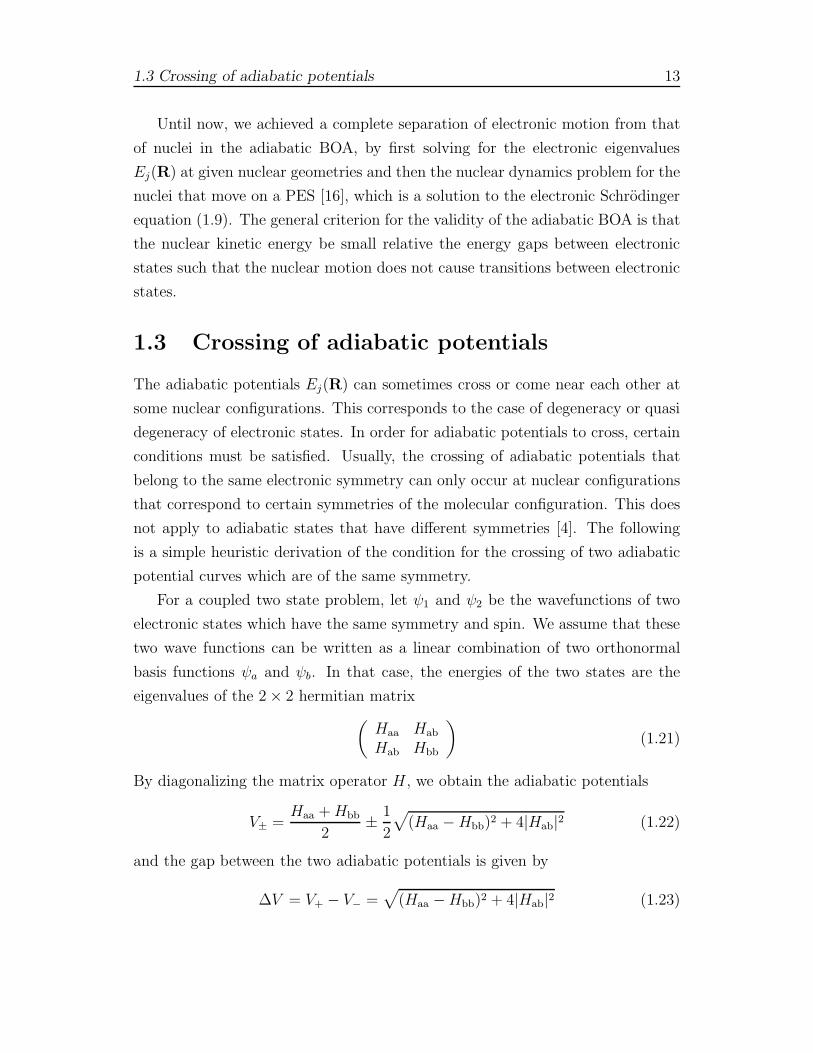
The adiabatic potentials Ej(R) can sometimes cross or come near each other at
some nuclear configurations. This corresponds to the case of degeneracy or quasi
degeneracy of electronic states. In order for adiabatic potentials to cross, certain
conditions must be satisfied. Usually, the crossing of adiabatic potentials that
belong to the same electronic symmetry can only occur at nuclear configurations
that correspond to certain symmetries of the molecular configuration. This does
not apply to adiabatic states that have different symmetries [4]. The following
is a simple heuristic derivation of the condition for the crossing of two adiabatic
potential curves which are of the same symmetry.
For a coupled two state problem, let ψ1 and ψ2 be the wavefunctions of two
electronic states which have the same symmetry and spin. We assume that these
two wave functions can be written as a linear combination of two orthonormal
basis functions ψa and ψb. In that case, the energies of the two states are the
eigenvalues of the 2 × 2 hermitian matrix
(Haa Hab
Hab Hbb
)(1.21)
By diagonalizing the matrix operator H , we obtain the adiabatic potentials
V± =Haa +Hbb
2± 1
2
√(Haa −Hbb)2 + 4|Hab|2 (1.22)
and the gap between the two adiabatic potentials is given by
∆V = V+ − V− =√
(Haa −Hbb)2 + 4|Hab|2 (1.23)
14 Concept of potential energy surface
For two adiabatic potentials to cross, the two positive terms in (1.23) must satisfy
the following equations simultaneously
{Haa(R) = Hbb(R)Hab(R) = 0
(1.24)
If ψa and ψb have different symmetries then Hab will be zero for all values of R.
In that case there may be a point or points at which (1.24) is satisfied, i.e. the
energies of two states are equal. These points will then be crossing points of the
potential energy curves [2, 17, 18].
1.4 Features of potential energy surface
The stationary points are the most important features of a PES, which have zero
gradient components (∂V/∂ρk = 0). These stationary points can be of several
types, depending on the second derivatives of the potential energy. The second
order derivatives of the potential energy at a stationary point can be expressed,
in terms of the internal coordinates ρi, as the (3N−6)× (3N−6) Hessian matrix
with elements defined by
∂2V/∂ρi∂ρj (1.25)
If all eigenvalues of the Hessian matrix are positive, the stationary point is a
minimum on the surface, at which an infinitesimal step in any direction leads
to an increase in potential energy. The minimum may correspond to reactants,
products or intermediates. Likewisely, maxima on the surface has all the negative
eigenvalues of the Hessian matrix, at which an infinitesimal step in any direction
leads to a decrease in potential. However, maxima are not generally of special
physical significance.
Saddle points are of particular interest in chemical kinetics because they lie
on the paths between points on the surface identified with reactant molecules
and points on the surface identified with product molecules. A saddle point is
the highest point on the path which involves the lowest increase in the potential
on passing from reactants to products. Stationary points also exist which have
more than one negative curvature along the principal axes. If there are k negative
second order derivative, then it is called k-th order saddle point. However, these
1.4 Bibliography 15
do not generally have any special kinetic significance because once a transition
state has been located, it should be verified that it indeed connects the desired
minima. At the saddle point, the vibrational normal coordinate associated with
the imaginary frequency is the reaction coordinate, and an inspection of the
corresponding atomic motion may be a strong indication that it is the correct
transition state.
Many methods are developed to locate stationary points on PESs, such as
Refs. [19–24] and the references cited therein.
Bibliography
[1] A. J. C. Varandas, Conical Intersections Electronic Structure, Dynamics and
Spectroscopy (World Scientific, 2004), chap. Modeling and interpolation of
global multi-sheeted potential energy surfaces, p. 205.
[2] J. N. Murrell, S. Carter, S. C. Farantos, P. Huxley, and A. J. C. Varandas,
Molecular Potential Energy Functions (Wiley, Chichester, 1984).
[3] A. J. C. Varandas, in Lecture Notes in Chemistry , edited by A. Lagana and
A. Riganelli (Springer, Berlin, 2000), vol. 75, pp. 33–56.
[4] J. Z. H. Zhang, Theory and Applications of Quantum Molecular Dynamics
(World Scientific, Singapore, 1999).
[5] A. J. C. Varandas, Int. Rev. Phys. Chem. 19, 199 (2000).
[6] M. Born and J. R. Oppenheimer, Ann. Phys. 84, 457 (1927).
[7] C. J. Cramer, Essentials of Computational Chemistry: Theories and Models
(John Wiley & Sons, 2004).
[8] A. S. Davidov, Quantum Mechanics (Pergamon, Oxford, 1965).
[9] H. Eyring and S. H. Lin, in Physical Chemistry, An Advanced Treatise, Vol.
VIA, Kinetics of Gas Reactions, edited by H. Eyring, D. Henderson, and
W. Jost (Academic, New York, 1974), p. 121.

16 Concept of potential energy surface
[10] R. Jaquet, Potential Energy Surfaces (Springer, 1999), chap. Interpolation
and fitting of potential energy surfaces, Lecture Notes in Chemistry.
[11] M. Piris, Fısica Cuantica (Editorial ISCTN, La Habana, 1999).
[12] F. Jensen, Introduction to Computational Chemistry (John Wiley & Sons,
2007).
[13] A. Messiah, Quantum Mechenics (Wiley, New York, 1966).
[14] M. Born and K. Huang, Dynamical Theory of Crystal Lattices (Clarendon
Press, Oxford, 1954).
[15] A. C. Hurley, Introduction to the Electron Theory of Small Molecules (Aca-
demic Press: London, 1976).
[16] N. C. Handy and A. M. Lee, Chem. Phys. Lett. 252, 425 (1996).
[17] C. A. Mead, J. Chem. Phys. 70, 2276 (1982).
[18] H. C. Longuet-Higgins, Proc. R. Soc. Ser. A 344, 147 (1975).
[19] H. B. Schlegel, Ab Initio Meth. Quant. Chem. I, 249 (1987).
[20] T. Schlick, Rev. Comput. Chem 3, 1 (1992).
[21] M. L. McKee and M. Page, Rev. Comput. Chem 4, 35 (1993).
[22] R. Fletcher, Practical Methods of Optimization (Wiley, Chichester, 1987).
[23] J. D. Head, B. Weiner, and M. C. Zerner, Int. J. Quantum Chem. 33, 177
(1988).
[24] K. Bondensgard and F. Jensen, J. Chem. Phys. 104, 8025 (1996).
Chapter 2
Calculation and representation ofpotential energy surface
The potential energy surface (PES), which is indeed a function obtained by fitting
to the ab initio energies, should describe the molecular energy as the internuclear
distance is changing continuously. Ab initio energies used to map a PES can be
gathered by solving the electronic problem represented in (1.9). Methods aimed
at solving (1.9) are broadly referred to the electronic structure calculation [1] and
significant advances have been made over many years [2] in the accurate ab initio
evaluation of the molecular energy within the Born-Oppenheimer approximation
(BOA) [3, 4]. The most common type of ab initio calculation is the Hartree-Fock
(HF) calculation [5, 6]. At higher levels of approximation, the quality of the wave
function is improved, so as to yield more and more elaborate solutions.
A large number of ab initio methods are available in many package program
to perform high level electronic structure calculations, such as Gaussian03 [7],
GAMESS [8] and Molpro [9]. In the following sections, a brief discussion of ab
initio methods, adopted for the calculation of PESs is presented.
2.1 Hartree-Fock theory
This section is divided into two parts. In the first part, the formula for the
expectation value E = 〈ΦA|He|ΦA〉 is deduced for the case in which ΦA is a
Slater determinant. While in the second part we derive the HF equation by
minimizing the expectation value E. Detailed treatments of the derivation of the
18 Calculation and representation of potential energy surface
HF equations may be found in Refs. [5, 6].
2.1.1 Derivation of the expectation value
HF theory is one of the simplest approximate theories for solving the many-body
Hamiltonian. For a molecular system consisting of N electrons and Nn nuclei,
the electronic Hamiltonian for a fixed nuclear configuration can be written as
He =
N∑
i
h(i) +1
2
∑
i6=j
1
rij(2.1)
where the second term represents the electron-electron interaction Vee and the
one electron Hamiltonian is given by:
h(i) = −1
2∇2
i +Nn∑
k
Zk
rik(2.2)
where rik = |ri − Rk|, rij = |ri − rj| and Zk is the electric charge of the kth
nucleus. Thus, (1.9) becomes:
(N∑
i
h(i) +1
2
∑
i6=j
1
rij
)φn(r) = Enφn(r) (2.3)
where the dependence of h(i), En and φn on R has been omitted for clarity and
nuclear-nuclear interactions have also been excluded.
It is not feasible to solve (2.3) exactly, as it is a complex many body problem.
Thus, usually further approximations are needed. One of the most important ap-
proximations in solving the electron problem is the HF approximation. The basic
idea of the HF approximation is as follows. It is well known that we can get the
exact solution of the electronic problem for the simplest atom, hydrogen, which
has only one electron. We imagine that if we add another electron to hydrogen, to
obtain H−. Assuming that the electrons do not interact with each other (i.e., that
Vee = 0), then the Hamiltonian would be separable. Thus, the total electronic
wavefunction φ(r1; r2) describing the motions of the two electrons can be written
as the product of two hydrogen atom wavefunctions, ψH(r1)ψH(r2). In the same
way, for the general problem, the electron wavefunction φ is approximated by the
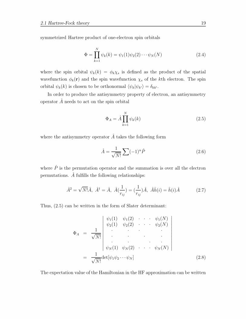
2.1 Hartree-Fock theory 19
symmetrized Hartree product of one-electron spin orbitals
Φ =
N∏
k=1
ψk(k) = ψ1(1)ψ2(2) · · ·ψN(N) (2.4)
where the spin orbital ψk(k) = φkχs is defined as the product of the spatial
wavefunction φk(r) and the spin wavefunction χs of the kth electron. The spin
orbital ψk(k) is chosen to be orthonormal 〈ψk|ψk′〉 = δkk′.
In order to produce the antisymmetry property of electron, an antisymmetry
operator A needs to act on the spin orbital
ΦA = A
N∏
k=1
ψk(k) (2.5)
where the antisymmetry operator A takes the following form
A =1√N !
∑(−1)αP (2.6)
where P is the permutation operator and the summation is over all the electron
permutations. A fulfills the following relationships:
A2 =√N !A, A† = A, A(
1
rij) = (
1
rij)A, Ah(i) = h(i)A (2.7)
Thus, (2.5) can be written in the form of Slater determinant:
ΦA =1√N !
∣∣∣∣∣∣∣∣∣∣∣∣
ψ1(1) ψ1(2) · · · ψ1(N)ψ2(1) ψ2(2) · · · ψ2(N)
· · · ·· · · ·· · · ·
ψN (1) ψN (2) · · · ψN(N)
∣∣∣∣∣∣∣∣∣∣∣∣
=1√N !
det[ψ1ψ2 · · ·ψN ] (2.8)
The expectation value of the Hamiltonian in the HF approximation can be written
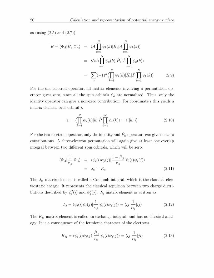
20 Calculation and representation of potential energy surface
as (using (2.5) and (2.7))
E = 〈ΦA|He|ΦA〉 = 〈AN∏
k=1
ψk(k)|He|AN∏
k=1
ψk(k)〉
=√n!〈
N∏
k=1
ψk(k)|He|AN∏
k=1
ψk(k)〉
=∑
α
(−1)α〈N∏
k=1
ψk(k)|He|PN∏
k=1
ψk(k)〉 (2.9)
For the one-electron operator, all matrix elements involving a permutation op-
erator gives zero, since all the spin orbitals ψk are normalized. Thus, only the
identity operator can give a non-zero contribution. For coordinate i this yields a
matrix element over orbital i.
εi = 〈N∏
k=1
ψk(k)|hi|PN∏
k=1
ψk(k)〉 = 〈i|hi|i〉 (2.10)
For the two-electron operator, only the identity and Pij operators can give nonzero
contributions. A three-electron permutation will again give at least one overlap
integral between two different spin orbitals, which will be zero.
〈ΦA|1
rij|ΦA〉 = 〈ψi(i)ψj(j)|
1 − Pij
rij|ψi(i)ψj(j)〉
= Jij −Kij (2.11)
The Jij matrix element is called a Coulomb integral, which is the classical elec-
trostatic energy. It represents the classical repulsion between two charge distri-
butions described by ψ2i (i) and ψ2
j (j). Jij matrix element is written as
Jij = 〈ψi(i)ψj(j)|1
rij|ψi(i)ψj(j)〉 = 〈ij| 1
rij|ij〉 (2.12)
The Kij matrix element is called an exchange integral, and has no classical anal-
ogy. It is a consequence of the fermionic character of the electrons.
Kij = 〈ψi(i)ψj(j)|Pij
rij|ψi(i)ψj(j)〉 = 〈ij| 1
rij|ji〉 (2.13)
2.1 Hartree-Fock theory 21
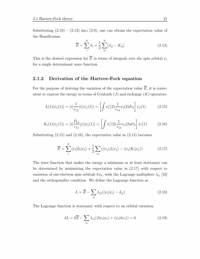
Substituting (2.10) – (2.13) into (2.9), one can obtain the expectation value of
the Hamiltonian
E =
N∑
i
hi +1
2
N∑
ij
[Jij −Kij] (2.14)
This is the desired expression for E in terms of integrals over the spin orbital ψi
for a single determinant wave function.
2.1.2 Derivation of the Hartree-Fock equation
For the purpose of deriving the variation of the expectation value E, it is conve-
nient to express the energy in terms of Coulomb (J) and exchange (K) operators.
Ji(1)|ψj(1)〉 = 〈i| 1
r12|i〉|ψj(1)〉 =
[∫ψ∗
i (2)1
r12ψi(2)dτ2
]ψj(1) (2.15)
Ki(1)|ψj(1)〉 = 〈i| P12
r12|j〉|ψj(1)〉 =
[∫ψ∗
i (2)1
r12ψj(2)dτ2
]ψi(1) (2.16)
Substituting (2.15) and (2.16), the expectation value in (2.14) becomes
E =
N∑
i
〈ψi|hi|ψi〉 +1
2
∑
ij
(〈ψj |Ji|ψj〉 − 〈ψj |Ki|ψj〉) (2.17)
The wave function that makes the energy a minimum or at least stationary can
be determined by minimizing the expectation value in (2.17) with respect to
variation of one-electron spin orbitals δψk, with the Lagrange multipliers λij [10]
and the orthogonality condition. We define the Lagrange function as
L = E −∑
ij
λij(〈ψi|ψi〉 − δij) (2.18)
The Lagrange function is stationary with respect to an orbital variation
δL = δE −∑
ij
λij(〈δψi|ψi〉 + 〈ψi|δψi〉) = 0 (2.19)
22 Calculation and representation of potential energy surface
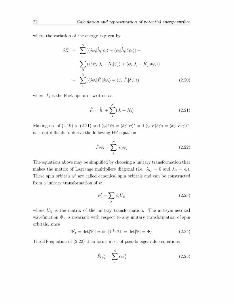
where the variation of the energy is given by
δE =
N∑
i
(〈δψi|hi|ψi〉 + 〈ψi|hi|δψi〉) +
∑
ij
(〈δψj |Ji −Ki|ψj〉 + 〈ψi|Jj −Kj |δψi〉)
=N∑
i
(〈δψi|Fi|δψi〉 + 〈ψi|Fi|δψi〉) (2.20)
where Fi is the Fock operator written as
Fi = hi +
N∑
i
(Ji −Ki) (2.21)
Making use of (2.19) to (2.21) and 〈ψ|δψ〉 = 〈δψ|ψ〉∗ and 〈ψ|F |δψ〉 = 〈δψ|F |ψ〉∗,it is not difficult to derive the following HF equation
Fiψi =N∑
j
λijψj (2.22)
The equations above may be simplified by choosing a unitary transformation that
makes the matrix of Lagrange multipliers diagonal (i.e. λij = 0 and λii = ǫi).
These spin orbitals ψ′ are called canonical spin orbitals and can be constructed
from a unitary transformation of ψ.
ψ′i =
∑
j
ψiUji (2.23)
where Uij is the matrix of the unitary transformation. The antisymmetrized
wavefunction ΦA is invariant with respect to any unitary transformation of spin
orbitals, since
Φ′A = det|Ψ′| = det|U†ΨU| = det|Ψ| = ΦA (2.24)
The HF equation of (2.22) then forms a set of pseudo-eigenvalue equations
Fiψ′i =
N∑
i
ǫiψ′i (2.25)
2.2 Koopmans’ theorem 23
A set of functions that are a solution to (2.25) are called self-consistent field
(SCF) orbitals. The orbital energy ǫi derived from the above equations is
ǫi = 〈ψ′i|ǫi|ψ′
i〉 = hi +
N∑
j
(Jij −Kij) (2.26)
The total energy can be written either as (2.9) or in terms of HF orbital energies
ǫi
E =N∑
i
ǫi −1
2
N∑
ij
(Jij −Kij) (2.27)
The total electronic energy is not simply a sum of HF orbital energies. The Fock
operator contains terms describing the repulsion to all other electrons and the
sum over spin orbital energies, therefore counts the electron-electron repulsion
twice which must be corrected for.
Although HF theory often gives useful and even accurate results for quantities
like equilibrium geometries of molecules, it neglects correlation between electrons
by assuming a single-determinant form for the wavefunction. The electrons are
subject to an average potential arising from the other electrons, which neglects
the instantaneous or correlated motions of electrons. It is useful to define the
difference between the exact energy of the electron system and HF energy as
electron correlation energy.
2.2 Koopmans’ theorem
It is still possible to relate ǫi to physical measurements, although the fact that
the total energy is not given by the sum of HF orbital energies. If certain assump-
tions are made, we are able to equate orbital energies with molecular ionization
energies or electron affinities. This identification is related to a theorem due to
Koopmans [11]. For a neutral molecular containing N electrons, the total energy
in the HF approximation is given by (2.27) and we write it again here.
ENg =
N∑
i
ǫi −1
2
N∑
ij
(Jij −Kij) (2.28)
24 Calculation and representation of potential energy surface
If one electron is removed from the kth orbital, the remaining N − 1 electrons
remain unchanged, the HF energy for this N − 1 electron system is given by
EN−1k =
N∑
i6=k
ǫi −1
2
N∑
i6=k,j 6=k
(Jij −Kij)
= ENg − hk −
1
2
N∑
i
(Jik −Kik) − 1
2
N∑
j
(Jkj −Kkj)
= ENg −
[hk +
N∑
j
(Jkj −Kkj)
](2.29)
because Jik = Jki and Kik = Kki. Subtracting the two total energies given by
(2.28) and (2.29), we can obtain the ionization energy (IE) [12] from the kth
orbital
IE = ENg − EN−1
k = hk +
N∑
j
(Jkj −Kkj) = εk (2.30)
As seen from (2.27), this is exactly the orbital energy εk. Similarly, the elec-
tron affinity (EA) of a neutral molecule is given as the orbital energy of the
corresponding anion, i.e. the energy for adding an extra electron to the sth
unoccupied orbital
EA = EN+1s −EN
g = εs (2.31)
(2.30) and (2.31) are the result known as Koopmans’ theorem [11], which gives
physical meaning to orbital energies and thus a means of calculation approximate
ionization energies and electron affinities. However, the theorem is very approxi-
mate [13]. First, the Koopermans’ theorem assumes that spin orbitals are frozen
after losing or adding an electron. In reality, the spin orbitals will relax and the
optimized orbitals will be different from the original ones after losing or adding an
electron. Secondly, the Koopermans’ theorem is based on the HF approximation
and neglects electron correlations.
2.3 Configuration interaction method
Configuration interaction (CI) [14] is one of the most general ways to improve
upon HF theory by adding a description of the correlations between electron
2.3 Configuration interaction method 25
motions. CI uses a variational wave function that is a linear combination [15] of
configuration state functions (CSFs) built from HF spin orbitals
Φ =∑
k
ckΦk (2.32)
In order to keep track of all the possible HF orbitals, we often write the
ground-state HF wave function as Φ0, the Slater determinant with an electron
“excited” from the ith occupied orbital to the ath unoccupied orbital as Φai , the
“doubly-excited” Slater determinants as Φabij , etc.. With this notation, we can
rewrite the wave function in (2.32) as
Φ = c0Φ0 +
N∑
i=1
M∑
a=N+1
cai Φai +
N∑
i>j=1
M∑
a>b=N+1
cabij Φab
ij + · · · (2.33)
where N is the number of electrons, so M is the total number of the HF orbitals.
Sometimes, it is helpful to abbreviate the indices on the Slater determinants
by introducing vectors, i and a, whose components are the orbitals from which an
electron is removed (i1, i2, . . .) and the orbitals to which it is excited (a1, a2, . . .),
respectively. By convention, the (2.33) is written as the form
Φ = c[1,2,...N ][1,2,...N ]Φ
[1,2,...N ][1,2,...N ] +
N∑
i1=1
M∑
a=N+1
c[a1,i2,...iN ][i1,i2,...iN ] Φ
[a1,i2,...iN ][i1,i2,...iN ]
+N∑
i1>i2=1
M∑
a1>a2=N+1
c[a1,a2,...iN ][i1,i2,...iN ] Φ
[a1,a2,...iN ][i1,i2,...iN ] + · · · =
∑
i,a
cai Φai (2.34)
To compute the configuration interaction wave function, we start with the
Shrodinger equation HΦ = EΦ. We then left multiply a Slater determinant Φai
to the both sides of the Shrodinger equation
Φai HΦ = Φa
iEΦ (2.35)
Substituting the (2.34) into the above equation, one gets
Φai H∑
j,b
cbjΦbj = Φa
iE∑
j,b
cbjΦbj (2.36)
and integrate the (2.36), we can obtain∑
j,b
〈Φai |H|Φb
j〉cbj = E∑
j,b
〈Φai |Φb
j〉cbj = E∑
j,b
δijδabcbj = Ecai (2.37)
26 Calculation and representation of potential energy surface
If we define the Hamiltonian matrix as Ha,b
i,j = 〈Φai |H|Φb
j〉, then the CI procedure
leads to a general matrix eigenvalue equation and (2.37) becomes
∑
j,b
Ha,b
i,j cbj = Ecai (2.38)
The solution of the CI procedure are the eigenvalues E and their corresponding
eigenvectors cai .
Configuration interaction calculations are classified by the number of excita-
tions used to make each determinant. When we truncate at zeroth-order, we have
the HF approximation [5, 6]. At first order, we have only one electron has been
moved for each determinant, it is called a Configuration Interaction with Single
excitation (CIS) [1]. CIS calculations give an approximation to the excited states
of the molecule, but do not change the ground state energy. At second order, we
have Configuration Interaction with Single and Double excitation (CISD) [1, 16]
yielding a ground-state energy that has been corrected for correlation. Triple-
excitation (CISDT) [1] and quadruple-excitation(CISDTQ) [1] calculations are
done only when very high accuracy results are desired. When we include all
possible excitations, we say that we are doing a Full Configuration Interaction
calculation, which is called Full CI (FCI) [15]. The number of all the possible ex-
citations is given by the number of determinants in an FCI wave function, which
has the following expression [12]
Ntot =
(M
N
)=
M !
N !(M −N)!(2.39)
For sufficiently large M , the FCI calculation will give an essentially exact result.
However, full CI calculations are rarely done due to the immense amount of
computer power required. For most applications, the CIS and CISD can give
good description of the electronic correlation energy.
2.4 Multiconfigurational SCF method
The Multiconfigurational Self Consistent Field (MCSCF) [17–19] method can be
considered a combination between the CI method (where the molecular orbitals
are not varied but the expansion of the wave functions) and the HF approximation
2.5 Multireference CI method 27
(where there is only one determinant but the molecular orbitals are varied). Si-
multaneous optimization of two sets of parameters is a difficult nonlinear problem,
and in practice severely restricts the length of the MCSCF expansions relative to
those of CI wave functions. Then, a compromise appears between generation of a
configuration space sufficiently flexible to describe the molecular system and the
number of variables to be computationally tractable.
A successful approach to select the MCSCF configurations is to partition
the molecular orbital space into three subspaces, containing inactive, active and
virtual (or unoccupied) orbitals respectively, which is known as the complete
active space self-consistent field (CASSCF) method [18, 19]. Typically, the core
orbitals of the system are treated as inactive and the valence orbitals as active.
Thus, the complete active space (CAS) consists in all configurations obtained
by distributing the valence electrons in all possible ways in the active orbitals,
keeping the core orbitals doubled occupied in all configurations, which is usually
called full valence complete active space (FVCAS) [19]. The configuration so
obtained is often referred to as reference configuration and the corresponding
space spanned is called the reference space.
In a CASSCF wave function, a part of the electronic correlation is covered,
called static or nondynamical correlation which arise from the strong interaction
between configurations nearly degenerated and is unrelated to the instantaneous
repulsion between the electrons. This last energy contribution constitutes the dy-
namical correlation energy. For high accuracy treatment of dynamical correlation,
additional calculations must be carried out based on the initial MCSCF method,
such as multirefernce CI (MRCI) method [20–24], which has been extensively
employed in this thesis.
2.5 Multireference CI method
The multireference configuration interaction (MRCI) method is a powerful one
to calculate accurate PESs. The general form of the MRCI method is MRCISD,
which includes only all the single and double excitations, i.e., neglects configura-
tions with more than two electrons in external orbitals. Its wavefunction can be
28 Calculation and representation of potential energy surface
written as [25]
|Ψ〉 =∑
I
CI |ΨI〉 +∑
S
∑
a
CSa |Ψa
S〉 +∑
P
∑
ab
CPab|Ψab
P 〉 (2.40)
where a and b refer to external orbitals, i.e., those not occupied in the reference
configurations, I denotes an orbital configuration with N electrons in the internal
orbital space while S and P denote internal N − 1 and N − 2 electronic hole
states [25–27]. |ΨI〉, |ΨaS〉 and |Ψab
P 〉 are internal, singly external and doubly
external configurations containing 0, 1, 2 occupied external orbitals, respectively.
Since there are usually many more external orbitals than internal ones, the
double external CSF’s |ΨabP 〉 are the most numerous in (2.40). If this number
is denoted as NP and the number of external orbitals denoted as N , then the
number of operations per iteration is proportional to NPN4 + Nx
pN3 [25], where
1 < x < 2. For this reason, it is difficult to perform uncontracted MRCI calcu-
lations with large reference configuration spaces (and large basis sets) which is
generated by two electron excitations from each individual reference configura-
tion. In order to reduce the computational effort, different contraction schemes
have been proposed [25, 28–31]. In the hybrid internally contracted MRCI (ICM-
RCI) [23, 25, 32], the internal configurations Ψklij and singly external configura-
tions Ψkaij are not contracted, while the doubly external configurations Ψab
ij are
contracted.
Using the configuration basis defined above, the total wavefunction maybe
written as [33]
|Ψ〉 =∑
I
CI |ΨI〉 +∑
S
∑
a
CSa |Ψa
S〉 +∑
ω=±1
∑
ab
∑
t≥u
Ctu,ωab |Ψab
tu,ω〉 (2.41)
where Ctu,ωab = ωCtu,ω
ba and the internally contracted doubly external configurations
are defined as
|Ψabtu,ω〉 =
1
2
(Eat,bu + ωEbt,au
)|Ψref〉 (2.42)
where ω = 1 for external singlet pairs and ω = −1 for external triplet pairs, and
|Ψref〉 is a reference wavefunction, which may be composed of many configurations
|Ψref〉 =∑
R
αR|ΨR〉 (2.43)
2.5 Multireference CI method 29
The internally contracted configurations |Ψabtu,w〉 can be expanded in terms of
the set of standard uncontracted doubly external CSFs |Ψabp 〉 according to
|Ψabtu,ω〉 =
∑
P
〈ΨabP |Ψab
tu,ω〉|ΨabP 〉 (2.44)
where the contraction coefficients are given by
〈ΨabP |Ψab
tu,ω〉 =1
2
∑
R
αR〈ΨabP |Eat,bu + ωEbt,au|ΨR〉 (2.45)
showing that these configurations are obtained by contracting different internal
states.
The configurations in (2.42) can be orthogonalized using the overlap matrix
S(ω) with its elements given by
S(ω)tu,rs = 〈Ψref |Etr,us + ωEts,ur|Ψref〉 (2.46)
so that the new orthonormal basis is obtained as
|ΨabD,ω〉 =
∑
t≥u
T(ω)D,tu|Ψab
tu,ω〉 T(ω) = (S(ω))−1/2 (2.47)
Substituting (2.47) into (2.41), the wavefunction becomes
|Ψ〉 =∑
I
CI |ΨI〉 +∑
S
∑
a
CSa |Ψa
S〉 +∑
ω=±1
∑
ab
∑
D
CD,ωab |Ψab
D,ω〉 (2.48)
This representation of the wavefunction is equivalent to (2.41), with D denotes
the orthogonalized internally contracted N − 2 electron states. The Hamiltonian
matrix can be diagonalized by using the popular procedure of Davidson [34–36],
which relies upon the formation of residual vectors that can then be used to
generate an updated vector of CI expansion coefficients. The residual vector can
be expressed as
〈ΨabD,ω|H −E|Ψ〉 =
{1
2
[GD,ω + ω(GD,ω)†
]−ECD,ω
}
ab
(2.49)
〈Ψas |H −E|Ψ〉 = (gs − ECs)a (2.50)
〈Ψas |H − E|Ψ〉 = gI −ECI (2.51)
The explicit formulas for the quantities GD,ω, gs and gI can be found in Refs. [23,
34, 37], which are calculated using an efficient direct CI method [34, 38].
30 Calculation and representation of potential energy surface
2.6 Møller-Plesset perturbation theory
In order to apply perturbation theory [39] to the calculation of the correlation
energy, the unperturbed Hamiltonian must be selected. The most common choice
is to take this as a sum over Fock operators [12], leading to Møller Plesset (MP)
perturbation theory [40–42], within which the unperturbed Hamiltonian is written
as
H0 =
N∑
i=1
Fi =
N∑
i=1
(hi +
N∑
j=1
gij
)=
N∑
i=1
hi +
N∑
i=1
N∑
j=1
gij (2.52)
where we write gij = (Jij − Kij) for simplicity. The perturbed Hamiltonian can
be expressed as
H =
N∑
i=1
hi +
N∑
i=1
N∑
j>i
gij (2.53)
So, we can write the perturbation as the difference between the perturbed and
unperturbed Hamiltonians.
H ′ = H − H0 =
N∑
i=1
N∑
j>i
gij −N∑
i=1
N∑
j=1
gij = −1
2
N∑
i=1
N∑
j=1
gij (2.54)
which is the difference between the instantaneous and average electron-electron
interaction. This perturbation is sometimes called the fluctuation potential as one
imagine that it measures the deviation from the mean of the electron interaction.
The zeroth-order wavefunction is the HF determinant, and the zeroth-order
energy is just a sum of one electron energies of the occupied spin orbitals
E(0) = 〈Ψ0|H0|Ψ0〉 = 〈Ψ0|N∑
i=1
Fi|Ψ0〉 =
N∑
i=1
ǫi (2.55)
The first order correction to the energy is the average of the perturbation over
the unperturbed wavefunction, which is given by
E(1) = 〈Ψ0|H ′|Ψ0〉 = −1
2
N∑
i=1
N∑
j=1
〈Ψ0|gij|Ψ0〉 = −1
2(Jij −Kij) (2.56)
Comparing (2.56) with the expression for the total energy in (2.27), it is seen
that the first-order energy (sum of E0 and E1) is exactly the HF energy. The
2.7 Coupled cluster theory 31
total energies MPn up to nth order can be written as
MP0 = E(0) =N∑
i=1
ǫi
MP1 = E(0) + E(1) = EHF (2.57)
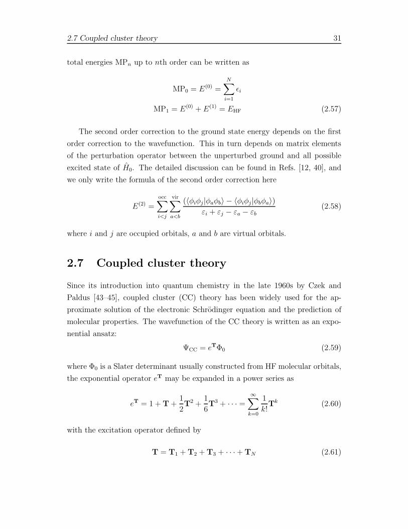
The second order correction to the ground state energy depends on the first
order correction to the wavefunction. This in turn depends on matrix elements
of the perturbation operator between the unperturbed ground and all possible
excited state of H0. The detailed discussion can be found in Refs. [12, 40], and
we only write the formula of the second order correction here
E(2) =
occ∑
i<j
vir∑
a<b
(〈φiφj|φaφb〉 − 〈φiφj|φbφa〉)εi + εj − εa − εb
(2.58)
where i and j are occupied orbitals, a and b are virtual orbitals.
2.7 Coupled cluster theory
Since its introduction into quantum chemistry in the late 1960s by Czek and
Paldus [43–45], coupled cluster (CC) theory has been widely used for the ap-
proximate solution of the electronic Schrodinger equation and the prediction of
molecular properties. The wavefunction of the CC theory is written as an expo-
nential ansatz:
ΨCC = eTΦ0 (2.59)
where Φ0 is a Slater determinant usually constructed from HF molecular orbitals,
the exponential operator eT may be expanded in a power series as
eT = 1 + T +1
2T2 +
1
6T3 + · · · =
∞∑
k=0
1
k!Tk (2.60)
with the excitation operator defined by
T = T1 + T2 + T3 + · · · + TN (2.61)
32 Calculation and representation of potential energy surface
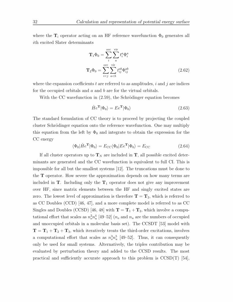
where the Ti operator acting on an HF reference wavefunction Φ0 generates all
ith excited Slater determinants
T1Φ0 =occ∑
i
vir∑
a
tai Φai
T2Φ0 =
occ∑
i<j
vir∑
a<b
tabij Φab
ij (2.62)
where the expansion coefficients t are referred to as amplitudes, i and j are indices
for the occupied orbitals and a and b are for the virtual orbitals.
With the CC wavefunction in (2.59), the Schrodinger equation becomes
HeT|Φ0〉 = EeT|Φ0〉 (2.63)
The standard formulation of CC theory is to proceed by projecting the coupled
cluster Schrodinger equation onto the reference wavefunction. One may multiply
this equation from the left by Φ0 and integrate to obtain the expression for the
CC energy
〈Φ0|HeT|Φ0〉 = ECC〈Φ0|EeT|Φ0〉 = ECC (2.64)
If all cluster operators up to TN are included in T, all possible excited deter-
minants are generated and the CC wavefunction is equivalent to full CI. This is
impossible for all but the smallest systems [12]. The truncations must be done to
the T operator. How severe the approximation depends on how many terms are
included in T. Including only the T1 operator does not give any improvement
over HF, since matrix elements between the HF and singly excited states are
zero. The lowest level of approximation is therefore T = T2, which is referred to
as CC Doubles (CCD) [46, 47], and a more complete model is referred to as CC
Singles and Doubles (CCSD) [46, 48] with T = T1 + T2, which involve a compu-
tational effort that scales as n2on
4u [49–52] (no and nu are the numbers of occupied
and unoccupied orbitals in a molecular basis set). The CCSDT [53] model with
T = T1 + T2 + T3, which iteratively treats the third-order excitations, involves
a computational effort that scales as n3on
5u [49–52]. Thus, it can consequently
only be used for small systems. Alternatively, the triples contribution may be
evaluated by perturbation theory and added to the CCSD results. The most
practical and sufficiently accurate approach to this problem is CCSD(T) [54],
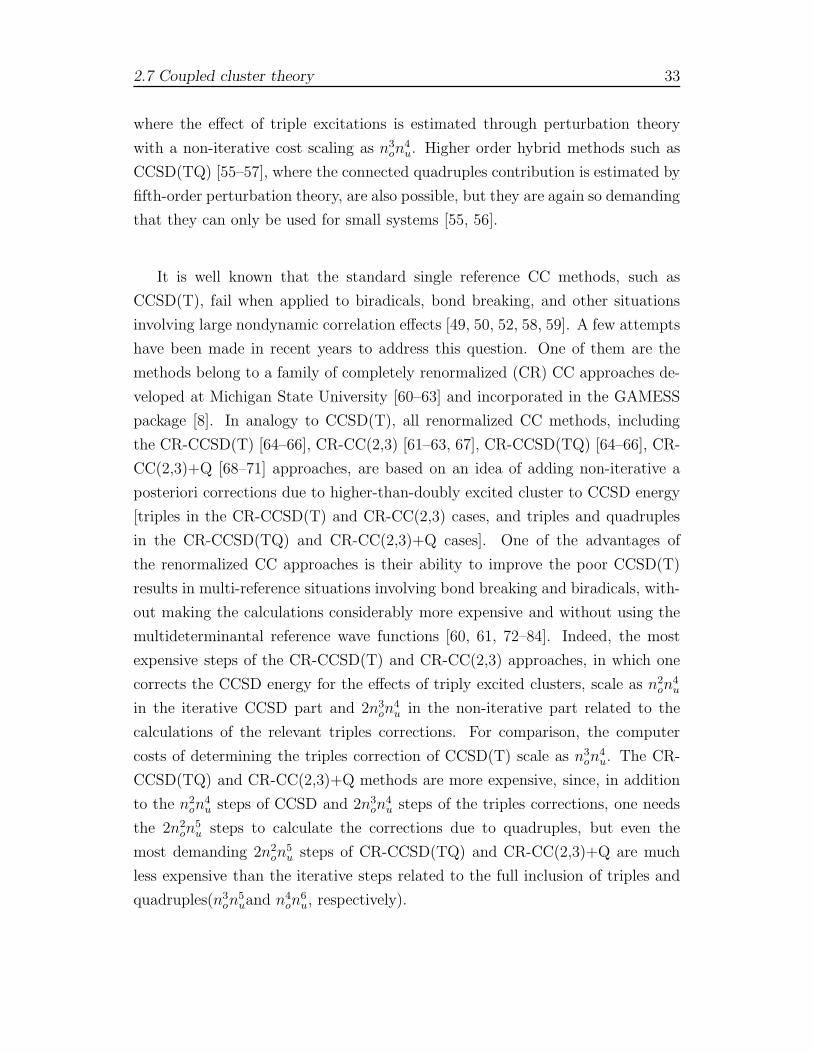
2.7 Coupled cluster theory 33
where the effect of triple excitations is estimated through perturbation theory
with a non-iterative cost scaling as n3on
4u. Higher order hybrid methods such as
CCSD(TQ) [55–57], where the connected quadruples contribution is estimated by
fifth-order perturbation theory, are also possible, but they are again so demanding
that they can only be used for small systems [55, 56].
It is well known that the standard single reference CC methods, such as
CCSD(T), fail when applied to biradicals, bond breaking, and other situations
involving large nondynamic correlation effects [49, 50, 52, 58, 59]. A few attempts
have been made in recent years to address this question. One of them are the
methods belong to a family of completely renormalized (CR) CC approaches de-
veloped at Michigan State University [60–63] and incorporated in the GAMESS
package [8]. In analogy to CCSD(T), all renormalized CC methods, including
the CR-CCSD(T) [64–66], CR-CC(2,3) [61–63, 67], CR-CCSD(TQ) [64–66], CR-
CC(2,3)+Q [68–71] approaches, are based on an idea of adding non-iterative a
posteriori corrections due to higher-than-doubly excited cluster to CCSD energy
[triples in the CR-CCSD(T) and CR-CC(2,3) cases, and triples and quadruples
in the CR-CCSD(TQ) and CR-CC(2,3)+Q cases]. One of the advantages of
the renormalized CC approaches is their ability to improve the poor CCSD(T)
results in multi-reference situations involving bond breaking and biradicals, with-
out making the calculations considerably more expensive and without using the
multideterminantal reference wave functions [60, 61, 72–84]. Indeed, the most
expensive steps of the CR-CCSD(T) and CR-CC(2,3) approaches, in which one
corrects the CCSD energy for the effects of triply excited clusters, scale as n2on
4u
in the iterative CCSD part and 2n3on
4u in the non-iterative part related to the
calculations of the relevant triples corrections. For comparison, the computer
costs of determining the triples correction of CCSD(T) scale as n3on
4u. The CR-
CCSD(TQ) and CR-CC(2,3)+Q methods are more expensive, since, in addition
to the n2on
4u steps of CCSD and 2n3
on4u steps of the triples corrections, one needs
the 2n2on
5u steps to calculate the corrections due to quadruples, but even the
most demanding 2n2on
5u steps of CR-CCSD(TQ) and CR-CC(2,3)+Q are much
less expensive than the iterative steps related to the full inclusion of triples and
quadruples(n3on
5uand n4
on6u, respectively).
34 Calculation and representation of potential energy surface
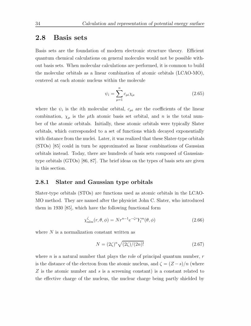
2.8 Basis sets
Basis sets are the foundation of modern electronic structure theory. Efficient
quantum chemical calculations on general molecules would not be possible with-
out basis sets. When molecular calculations are performed, it is common to build
the molecular orbitals as a linear combination of atomic orbitals (LCAO-MO),
centered at each atomic nucleus within the molecule
ψi =n∑
µ=1
cµiχµ (2.65)
where the ψi is the ith molecular orbital, cµi are the coefficients of the linear
combination, χµ is the µth atomic basis set orbital, and n is the total num-
ber of the atomic orbitals. Initially, these atomic orbitals were typically Slater
orbitals, which corresponded to a set of functions which decayed exponentially
with distance from the nuclei. Later, it was realized that these Slater-type orbitals
(STOs) [85] could in turn be approximated as linear combinations of Gaussian
orbitals instead. Today, there are hundreds of basis sets composed of Gaussian-
type orbitals (GTOs) [86, 87]. The brief ideas on the types of basis sets are given
in this section.
2.8.1 Slater and Gaussian type orbitals
Slater-type orbitals (STOs) are functions used as atomic orbitals in the LCAO-
MO method. They are named after the physicist John C. Slater, who introduced
them in 1930 [85], which have the following functional form
χζnlm(r, θ, φ) = Nrn−1e−ζrY m
l (θ, φ) (2.66)
where N is a normalization constant written as
N = (2ζ)n√
(2ζ)/(2n)! (2.67)
where n is a natural number that plays the role of principal quantum number, r
is the distance of the electron from the atomic nucleus, and ζ = (Z−s)/n (where
Z is the atomic number and s is a screening constant) is a constant related to
the effective charge of the nucleus, the nuclear charge being partly shielded by
2.8 Basis sets 35
electrons. It is common to use the spherical harmonics Y ml (r) depending on the
polar coordinates of the position vector r as the angular part of the Slater orbital.
The exponential dependence ensures a fairly rapid convergence with increasing
numbers of functions. However, the calculation of three- and four-center two-
electron integrals cannot be performed analytically [12]. Thus, STOs are only
used for atomic and diatomic systems where high accuracy is required, and in
semi-empirical methods where all three- and four-center integrals are neglected.
To speed up molecular integral evaluation, GTOs were first proposed by
Boys [86] in 1950, which can be written in terms of polar or Cartesian coor-
dinates as
χζnlm(r, θ, φ) = Nr2n−2−le−ζr2
Y ml (θ, φ)
χζlxly lz
(r, θ, φ) = Nxlxylyzlze−ζr2
(2.68)
The sum of the exponents of the Cartesian coordinates, l = lx + ly + lz, is used
to mark functions as s-type (l=0), p-type (l=1), d-type (l=2), and so on. The
main difference to the STOs is that the variable r in the exponential function is
squared. Thus, Gaussian Product Theorem [88] guarantees that the product of
two GTOs centered on two different atoms is a finite sum of Gaussians centered on
a point along the axis connecting them. In this manner, four-center integrals can
be reduced to finite sums of two-center integrals, and in a next step to finite sums
of one-center integrals. This speeds up by 4–5 orders of magnitude compared to
Slater orbitals more than outweighs the extra cost entailed by the larger number
of basis functions generally required in a Gaussian calculation.
However, GTOs have two major problems compared with STOs. First, GTOs
do not have a cusp at r = 0. The other problem is that GTOs fall off too rapidly
for large r. It is known from (2.68) that GTOs with large α are very much
concentrated around the origin (in the limit of infinite α they tend to a Dirac
delta function) and can mimic the correct cusp, while GTOs with small α are
very diffuse (spread out) and can describe the behavior of a molecular orbital
(MO) at large r. Thus, these problems can be corrected by linear combinations
of GTOs, which leads to the introduction of contracted sets of primitive GTOs
36 Calculation and representation of potential energy surface
(CGTOs) [89, 90], which take the following formation
χν =M∑
ν=1
dµνgν(αν) (2.69)
where M is the length of the contraction, the gν ’s are primitive Gaussians func-
tions, dµν and is contraction coefficients which can be determined by least-square
fits to accurate atomic orbital or by minimization of the total HF energy.
2.8.2 Classification of basis sets
Once the type of function (STO or GTO) is selected, the next step is to choose
the number of functions to be used. The smallest number of functions possible,
to contain all the electrons in a neutral atom, is called minimum basis set. Thus,
for hydrogen (and helium) it means a single s-function, for the first row elements
of the periodic table, it requires two s-functions (1s, 2s) and one set of p-functions
(2px, 2py, 2pz), and so on. The next improvement is to double all basis functions,
producing a Double zeta (DZ) type basis, which employs two s-functions for
hydrogen (1s and 1s′), four s and two p-functions for the elements on the first
row, and so on. One can also go further to Triple Zeta (TZ), Quadruple Zeta
(QZ), Quintuple Zeta (5Z) and so on.
Often it takes too much effort to calculate a DZ for every orbital. Instead,
many scientists simplify matters by calculating a DZ only for the valence orbital.
Since the inner-shell electrons are not as vital to the calculation, they are de-
scribed with a single Slater Orbital. This method is called a split-valence basis
set. The n − ijG or n − ijkG split-valence basis sets are due to Pople and co-
workers [91–93], where n is the number of primitives summed to describe the
inner shells, ij or ijk is the number of primitives for contractions in the valence
shell. In the 6 − 31G basis, for example, the core orbitals are described by a
contraction of six GTOs, whereas the inner part of the valence orbitals is a con-
traction of three GTOs and the outer part of the valence is represented by one
GTOs. Including polarization functions give more angular freedom so that the
basis is able to represent bond angles more accurately, especially in strained ring
molecules. For example, 6−31G∗∗ basis set, the first asterisk indicate the addition
of d functions on the non-hydrogen atoms and the second asterisk a p function
2.8 Basis sets 37
on hydrogen atom [94]. Another type of functions can be added to the basis for
a good description of the wavefunction far from the nucleus are the diffuse func-
tions, which are additional GTOs with small exponents. The diffuse functions
are usually indicated with a notation “+”. For example, in the 6-31++G basis
set, the ”++” means the addition of a set of s and p function to the heavy atoms,
while an additional s diffuse GTO for hydrogen.
For correlated calculations, the basis set requirements are different and more
demanding since we must then describe the polarizations of the charge distri-
bution and also provide an orbital space suitable for recovering correlation ef-
fects. For this purpose, the correlation consistent basis sets are very suited,
which is usually denoted as cc-pVXZ [95, 96]. The “cc” denotes that this is a
correlation-consistent basis, meaning that the functions were optimized for best
performance with correlated calculations. The “p” denotes that polarization func-
tions are included on all atoms. The“VXZ” stands for valence with the cardinal
number X = D, T,Q, . . . indicate double-, triple- or quadruple-zeta respectively.
The inclusion of diffuse functions, which can improve the flexibility in the outer
valence region, leads to the augmented correlation-consistent basis sets aug-cc-
pVXZ [95, 96], where one set of diffuse functions is added in cc-pVXZ basis.
2.8.3 Basis set superposition error
In quantum chemistry, calculations of molecular properties are all done using a
finite set of basis functions, which may lead to an important phenomenon referred
as the basis-set superposition error (BSSE) [97, 98]. As the atoms of interacting
molecules (or of different parts of the same molecule) approach one another, their
basis functions overlap. Each monomer ”borrows” functions from other nearby
components, effectively increasing its basis set and improving the calculation of
derived properties such as energy. If the total energy is minimized as a function of
the system geometry, the short-range energies from the mixed basis sets must be
compared with the long-range energies from the unmixed sets, and this mismatch
introduces an error. Other than using infinite basis sets, the counterpoise method
(CP) [99] is used to account for the BSSE. In the CP method, the BSSE is
calculated by re-performing all the calculations using the mixed basis sets, and
the error is then subtracted a posterior from the uncorrected energy. On the other
38 Calculation and representation of potential energy surface
hand, the BSSE can be corrected by scaling [100] or extrapolating [101–104] the
ab initio energies to the complete basis set limit as discussed in the next section.
2.9 Semiempirical correction of ab initio ener-
gies
2.9.1 Scaling the external correlation energy
The truncate CI wave function lacks of size-extensivity, as it does not include
as much of the dynamical or external electron correlation effects. A method to
incorporate semiempirically the external valence correlation energy was proposed
by Brown and Truhlar [105]. In such approach the non-dynamical (static) or
internal correlation energy is obtained by an MCSCF calculation and the part
of external valence correlation energy by an MRCISD calculation based on the
MCSCF wave functions as references. Then, it is assumed that the MRCISD
includes a constant (geometry independent) fraction F of the external valence
correlation energy, which can be extrapolated with the formula
ESEC (R) = EMCSCF (R) +EMRCISD (R) − EMCSCF (R)
F(2.70)
where ESEC (R) denotes the scaled external correlation (SEC) energy, and the
empirical factor F is chosen for diatomics to reproduce a bond energy, and for
systems with more atoms chosen to reproduce more than one bond energy in an
average sense [105].
As pointed out by these authors [105], the SEC method requires a large enough
MCSCF calculation and one-electron basis sets, in order to include dominant
geometry dependent internal correlation effects and an appreciable fraction of
the external valence correlation energy.
By including information relative to experimental dissociation energies, the
SEC method attempts to account for the incompleteness of the one-electron basis
set [106]. MRCISD calculation based on large enough basis set contributes to
minimize undesirable BSSE, which may be corrected subsequently by scaling the
external correlation energy.
Varandas [106] suggested a generalization of the SEC method by noticing the
conceptual relationship between it and the double many-body expansion (DMBE)
2.9 Semiempirical correction of ab initio energies 39
method [107]. In fact, in the DMBE scheme each n-body potential energy term is
partitioned into extended-Hartree-Fock (internal correlation) and dynamic corre-
lation (external correlation) parts. In his proposal, denoted as DMBE-SEC [106],
this author writes the total interaction energy, relative to infinitely separated
atoms in the appropriate electronic states, in the form
V (R) = VMCSCF (R) + VSEC (R) (2.71)
where
VMCSCF (R) =∑
V(2)AB,MCSCF (RAB) +
∑V
(3)ABC,MCSCF (RAB, RBC, RAC) + . . . (2.72)
VSEC (R) =∑
V(2)AB,SEC (RAB) +
∑V
(3)ABC,SEC (RAB, RBC, RAC) + . . . (2.73)
and the summations run over the subcluster of atoms (dimers, trimers, ...) which
compose the molecule.
The scaled external correlation energy component for the n-th terms is given
by
V(n)AB...,SEC =
V(n)AB...,MRCISD − V
(n)AB...,MCSCF
F (n)AB
(2.74)
where F (n)AB... is the n-body geometry independent scaling factor.
As in the original SEC method, optimal values for two-body factors F (2)AB are
chosen to reproduce experimental dissociation energies, a criterion which may
be adopted for higher-order terms if accurate dissociation energies exist for the
relevance subsystems [106]. For the triatomic case a good guess for F (3)ABC can be
the average of the two-body factors
F (3)ABC =
1
3
[F (2)
AB + F (2)BC + F (2)
AC
](2.75)
Improved agreement with experiment and best theoretical estimates, is ob-
tained when ab initio energies are corrected with the DMBE–SEC method. Par-
ticularly important, for dynamics calculations, are the correct exothermicities for
all arrangement channels, exhibited by the DMBE–SEC potential surfaces [106].
2.9.2 Extrapolation to complete basis set limit
The large majority of electronic structure calculations employ an expansion of
the orbitals in a basis set, almost always of the Gaussian type and located at the
40 Calculation and representation of potential energy surface
nuclear positions. The basis set incompleteness is one of the factors that limits
the ultimate accuracy. For small molecule, a significant enhancement to progress
in electronic structure calculations has become possible with the introduction of
correlation-consistent basis sets developed by Dunning [95]. The most common
family of Dunning basis sets are denoted as cc-pVXZ, especially the augmented
ones (aug-cc-pVXZ). More recently there has been much interest in exploiting
the systematic behavior of these basis sets with respect to the cardinal number
X by carrying out calculations for several values of X and extrapolating to the
complete basis set (CBS) limit. Much effort has been put onto the extrapolation
schemes to obtain the molecular energy at the CBS limit at a computational
cost as low as possible [96, 108–119]. In most recent articles [110–114], Varandas
proposed a practical scheme for extrapolating electronic energies calculated with
correlation consistent basis sets of Dunning. The MRCI(Q) electronic energy is
best treated in split form by writing [110]
EX(R) = ECAS(R) + Edc(R) (2.76)
where R specifies the three-dimensional vector of space coordinate, the subscript
X indicates that the energy has been calculated in the AVXZ basis and the su-
perscripts CAS and dc stand for complete-active space and dynamical correlation
energies, respectively. For CAS (uncorrelated in the sense of lacking dynamical
correlation energies), several schemes have been advanced [108–112]. To extrap-
olate Hartree-Fock energies using AVTZ and AVQZ basis sets, the most reliable
protocol is possibly the one due to Karton and Martin [108] denoted as KM(T,Q).
Our past experience [111] with AV5Z and AV6Z energies suggests that the same
protocol can be successfully utilized with the CAS energy component, hence we
will adopt the KM(T,Q) protocol in the present work. This assumes the form
ECASX (R) = ECAS
∞ (R) +B/Xα (2.77)
where α = 5.34 is an effective decay exponent.
To extrapolate the dynamic correlation (dc) energy, the uniform singlet- and
triplet-pair extrapolation (USTE) scheme [110] developed by Varandas has shown
great promise in extrapolating from (T,Q) cardinal-number pairs, which assumes
2.9 Semiempirical correction of ab initio energies 41
the following formation
EdcX (R) = Edc
∞(R) +A3
(X + α)3+
A5
(X + α)5(2.78)
with A5 being determined by the auxiliary relation
A5 = A5(0) + cA5/43 (2.79)
where A5(0) = 0.0037685459Eh, c = −1.17847713E−5/4h , and α = −3/8, with
E∞ and A3 are determined from a fit to the dc energies with the AVTdZ and
AVQdZ basis sets [110].
The computational cost can be further reduced by obtaining the dynamical
correlation energy at MRCI(Q)/AVQZ basis set via correlation scaling (CS) at
one [112] or more [113] pivotal geometries, heretofore denoted as CSN where N
is the number of pivots. It is the joint use of the CSN and USTE(T,Q) methods.
The full approach, hereafter called CSN/USTE(T,Q), involves six basic steps:
(a) calculation of the PES at Nt points with the X−2 and X−1 basis sets using
MRCI(Q), and N(= 1 − 4) such calculations with the target basis set of rank X
at the pivots; (b) calculation of all the considered geometries of the PES at the
CAS level with the target X basis set level; (c) extrapolation to the CBS limit
(i.e., X = ∞) of the CAS energies using (2.77); (d) prediction by extrapolation to
X = ∞ of the dc energy at the pivots by using (2.78); (e) prediction of the CBS
dc energies of the remaining Nt −N points by CS [112, 113] using the X = D, T
and CBS dc energies at the pivots; (f) calculation of the full CBS PES by adding
the CAS/CBS and extrapolated dynamical correlation energies from steps (c)–
(e). In case of single pivot, which is denoted by CS1/USTE(T,Q) method [112],
assumes the form
Edc(R)=χ∞,3(R)Edc3 (R) (2.80)
where the scaling function χ assumes the form
χ∞,3(R)=1 +S3,2(R) − 1
S3,2(Re) − 1[S∞,3(Re) − 1] (2.81)
where Re indicates the pivotal geometry, and
Sm,n(R)=Edc
m (R)
Edcn (R)
(2.82)
42 Calculation and representation of potential energy surface
Thus, CBS extrapolation via (2.80)–(2.82) utilizes the correlation energies calcu-
lated with AVDZ and AVTZ basis sets using a single pivotal geometry at which
the dc energy has also been calculated with the AVQZ basis set.
2.10 Analytical representation of potential en-
ergy surface
Once enough information on the potential energy of the system under study has
been gathered, it is necessary to present it in a realistic global functional form, in
order to carry out dynamics studies. Nevertheless, a choice of suitable function
is not an easy task. A successful representation of a global PES for dynamical
calculations should satisfy certain criteria, as discussed by Wright and Gray [120]
and remarked by Varandas [121]:
1. “It should accurately characterize the asymptotic reactant and product
molecules (or more generally any fragment of the full system).”
2. “It should have correct symmetry properties of the system.”
3. “It should represent the true PES in interaction regions for which experi-
mental or non-empirical theoretical data are available (including, in prin-
ciple, the very short-range and long-range regions associated with various
asymptotic channels [122]).”
4. “It should behave in a physically reasonable manner in those parts of the
interaction region for which no experimental or theoretical data are avail-
able.”
5. “It should smoothly connect the asymptotic and interaction region in a
physically reasonable way.”
6. “The function and its derivatives should have as simple an algebraic form
as possible consistent with the desired quality of the fit.”
7. “It should require as small a number of data points as possible to achieve
an accurate fit.”
2.10 Analytical representation of potential energy surface 43
8. “It should converge to the true surface as more data become available.”
9. “It should indicate where it is most meaningful to compute the data points.”
10. “It should have a minimal amount of ad hoc or ’patched up character’.”
Criteria from 1 to 5 must be obeyed in order to obtain reasonable results in
subsequent calculations using the function. Criteria from 6 to 10 are desirable
for practical reasons. Finding a function that meets these criteria requires skill
and experience, and considerable amount of patience [123].
Methods to construct analytical PESs have been developed for many years.
Among them are the semiempirical London-Eyring-Polanyi-Sato (LEPS) [124–
126] and diatomics-in-molecules (DIM) [127–129] methods, which use theoretical
and experimental information to fit a functional form derived from simple molecu-
lar orbital theory. A more general approach is the many-body expansion (MBE)
method developed by Murrel and co-workers [130–132], which proposed to de-
scribe the total interaction of the polyatomic system by adding all the many-body
interactions of each fragment. The PESs discussed in the present thesis are rep-
resented using an improved version of MBE due to Varandas [100, 107, 122, 133]:
the double many-body expansion (DMBE) method, which consists in partitioning
each n-body contribution in short-range and long-rang parts. The more detailed
discussion of MBE and DMBE methods is given in the following sections.
2.10.1 The many-body expansion method
The many-body expansion (MBE) for a single-valued PES of an N -atomic system
is written as [131]:
VABC···N(R) =∑
V(1)A +
∑V
(2)AB (RAB) +
∑V
(3)ABC(RAB, RAC, RBC) + · · ·
+V(N)ABC···N(R) (2.83)
where V(1)A is the energy of the atom A, and the summation runs over all the
one-body terms. If the reference energy is taken as the energy of all the atoms
in their ground states, then V(1)A will be zero. V
(2)AB (RAB) is a two-body energy
term, depending on the distance separating the two atoms, and which goes to
zero as RAB tends to infinity. V(3)ABC(RAB, RAC, RBC) is a three-body energy which
44 Calculation and representation of potential energy surface
depends on the three distances of the triangle ABC. The last term in the expan-
sion V(N)ABC···N(R) is the n-body energy. It depends, as the total potential function,
on the 3N − 6 internal coordinates.The MBE function is designed to satisfy all
dissociation limits, and it also provides a strategy for building up PESs of larger
polyatomic systems. Once the potentials of all the fragments are deduced, they
can be used in all the polyatomics containing such fragments.
2.10.2 The double many-body expansion method
MBE method is proposed to provide an analytical representation of PESs for all
possible configurations of the system. Then, its functional form must properly
reproduce all the regions, from short range interactions to long range ones. How-
ever, the method fails in keeping only one function to reproduce both ranges.
Thus, the idea of splitting each many-body terms into two parts arises. In such
spirit, Varandas [100, 107, 122, 133] extended the many-body expansion to the
double many-body expansion (DMBE) in which each many-body term is splitted
into two parts: one accounting for the long range or dynamical correlation (dc)
energy and the other describing the short range or extended-Hartree-Fock (EHF)
energies.
V (RN) =N∑
n=1
∑
Rn⊂RN
[V
(n)EHF(Rn) + V n
dc(Rn)]
(2.84)
where, Rn denotes any set of n(n−1)/2 coordinates of the fragment containing n
atoms, which is a subset of RN ≡ [R1, R2, . . .RN(N−1)/2], and last sum is carried
out over all such subsets.
In a series of papers Varandas and coworkers [107, 122, 134–137] proposed
general expressions for the n-body dynamic correlation energy term, to repro-
duce the proper anisotropy and asymptotic behavior of the PES for the entire
configuration space (for details see cases studies). An important result refers to
the introduction of an universal charge-overlap damping function to account for
the damping of the dispersion coefficients for intermediate and small interatomic
separations [134].
Extended Hartree-Fock approximate correlation energy for two- and three-
body interactions (EHFACE2 and EHFACE3) models have been proposed [135],
2.10 Analytical representation of potential energy surface 45
from simple, yet reliable, physical motivated forms. To represent the global short-
range energy for two-body potentials, a screened extended-Rydberg form (with an
extra R−1 term) can be adapted, which reproduces the exact ZAZB/R behavior
at the united atom limit (EHFACE2U model [137]). In turn, the three-body
EHF potential is represented by the following three-body distributed-polynomial
form [138]
V(3)EHF (R) =
m∑
i=1
P (i) (Q1, Q2, Q3)
3∏
j=1
{1 − tanh
[γ
(i)j
(Rj − Ri,ref
j
)]}(2.85)
where P (i) (Q1, Q2, Q3) are polynomials in the symmetric coordinates {Qk}, ex-
pressed as combinations of the internuclear coordinates {Rj}, which transform
as irreducible representations of the permutation group of the molecule [132]. In
turn, Ri,refj represents a convenient reference geometry to which the i-th com-
ponent of (2.85) is referred to [138]. If extensive ab initio data is available, the
optimized coefficients for the two-body and three-body terms can be obtained
using linear or non-linear least-square fits [139].
2.10.3 Approximate single-sheeted representation
When two or more potential energy surfaces cross, an exact treatment demands
a multi-sheeted representation of the PES. Such representation of the potential
can be expressed as the lowest eigenvalues of a square matrix of order equal to
the number of states involved [140]. Thus, the elements of the diabatic potential
matrix can be written as many-body expansions or double-many body expansions
involving the appropriate electronic states of the fragments.
However, for many situations an approximated single-sheeted representation
can provide a good analytical form for dynamical purposes. For example, if a
crossing between states is present, it can be avoided in such a way that the po-
tential function smooths the region around the intersection point. If the crossing
is located well above the dissociation channels or the stationary points of the
molecule, it is expected to have a minor influence in the dynamics of the system.
In the present work, DMBE potential energy surfaces for the systems H2S (1A′)
and HS2 (2A′′) were calibrated following this procedure. Further dynamics calcu-
lations using the obtained DMBE-PES for H2S were carried out for the reaction
46 Calculation and representation of potential energy surface
S (1D) + H2
(X 3Σ+
g
)→ SH (X 2Π)+ H (2S) showing the reliability of the approx-
imated single-sheeted form.
A single-sheeted representation uses switching functions to account for the
presence of different states of fragments for different regions of the configuration
space. The switching function was firstly applied by Murrel and Carter [141]
to construct a MBE PES for ground-state H2O. These authors introduced a
switching one-body term for oxygen, allowing that in the PES the atomic state
O (1D) is connected for the channel H2
(X1Σ+
g
)+ O (1D) and disconnected for
the other dissociation limits. A smooth description of the PES which accounted
for such a behavior of the oxygen atomic state, is warrant employing a switching
function in the form
f (x) =1
2[1 − tanh (αx)] (2.86)
which has the limits unity as x→ −∞ and zero as x→ +∞.
By choosing the variable x as
x = nρ3 − ρ1 − ρ2 (2.87)
where ρi = Ri − R0i are the displacements of the internuclear distances from a
reference structure (R3 the H–H distance, and R1, R2 the OH distance), then it
is easy to see that x takes the limit −∞ for dissociation into H2 + O and +∞ for
dissociation to OH + H provided n ≥ 2.
Although the function (2.86) shows a proper behavior for short and interme-
diate distances of the triatomic, it cannot reach a unique value at the three-atom
limit [141]. In fact, even for large H–H separation, the function (2.86) switches
from 0 to 1 when oxygen moves far away from the diatomic. To correct such
unphysical behavior, Varandas and Poveda [142] have suggested an improved
switching function in their work on DMBE PES of NH2(2A′′). The same func-
tional form is employed in the construction of an approximated single-valued
DMBE PES for H2S (X 1A′), which can be written as
V (R) = V(1)
S(1D)f(R) +3∑
i=1
V (2)(Ri) + V (3)(R) (2.88)
where V(1)
S(1D) represents the energy difference between the 1D and 3P states of
atomic sulfur, f(R) is the switching function used to warrant the correct behav-
ior at the H2(X1Σ+
g ) + S(1D) and SH(X 2Π) + H(2S) dissociation limits, while
2.10 Bibliography 47
V (2)(Ri) and V (3)(R) represent the two-body and three-body energy terms re-
spectively.
Bibliography
[1] T. Helgaker, P. Jørgensen, and J. Olsen, Molecular Electronic-Structure
Theory (Wiley, Chichester, 2000).
[2] J. Almlof, in Modern Electronic Structure Theory (World Scientific, Singa-
pore, 1995).
[3] A. C. Hurley, Introduction to the Electron Theory of Small Molecules (Aca-
demic Press: London, 1976).
[4] M. Born and J. R. Oppenheimer, Ann. Phys. 84, 457 (1927).
[5] C. C. J. Roothaan, Rev. Mod. Phys. 23, 69 (1951).
[6] J. A. Pople and D. L. Beveridge, Approximate Molecular Orbital Theory
(McGraw-Hill, New York, 1970).
[7] M. J. Frisch, G. W. Trucks, H. B. Schlegel, G. E. Scuseria, M. A. Robb,
J. R. Cheeseman, J. A. Montgomery, Jr., T. Vreven, K. N. Kudin, J. C.
Burant, J. M. Millam, S. S. Iyengar, J. Tomasi, V. Barone, B. Mennucci,
M. Cossi, G. Scalmani, N. Rega, G. A. Petersson, H. Nakatsuji, M. Hada,
M. Ehara, K. Toyota, R. Fukuda, J. Hasegawa, M. Ishida, T. Nakajima,
Y. Honda, O. Kitao, H. Nakai, M. Klene, X. Li, J. E. Knox, H. P. Hratchian,
J. B. Cross, V. Bakken, C. Adamo, J. Jaramillo, R. Gomperts, R. E. Strat-
mann, O. Yazyev, A. J. Austin, R. Cammi, C. Pomelli, J. W. Ochterski,
P. Y. Ayala, K. Morokuma, G. A. Voth, P. Salvador, J. J. Dannenberg,
V. G. Zakrzewski, S. Dapprich, A. D. Daniels, M. C. Strain, O. Farkas,
D. K. Malick, A. D. Rabuck, K. Raghavachari, J. B. Foresman, J. V. Ortiz,
Q. Cui, A. G. Baboul, S. Clifford, J. Cioslowski, B. B. Stefanov, G. Liu,
A. Liashenko, P. Piskorz, I. Komaromi, R. L. Martin, D. J. Fox, T. Keith,
M. A. Al-Laham, C. Y. Peng, A. Nanayakkara, M. Challacombe, P. M. W.
48 Calculation and representation of potential energy surface
Gill, B. Johnson, W. Chen, M. W. Wong, C. Gonzalez, and J. A. Pople,
Gaussian 03, Revision C.02, Gaussian, Inc., Wallingford, CT, 2004.
[8] M. W. Schmidt, K. K. Baldridge, J. A. Boats, S. T. Elbert, M. S. Gorgon,
J. H. Jensen, S. Koseki, N. Matsunaga, K. A. Nguyen, S. Su, T. L. Windus,
M. Dupuis, and J. Montgomery, Jr., J. Comput. Chem. 14, 1347 (1993).
[9] H.-J. Werner and P. J. Knowles, MOLPRO is a package of ab initio pro-
grams written by H.-J. Werner, P. J. Knowles, with contributions from R.
D. Amos, A. Bernhardsson, A. Berning, P. Celani, D. L. Cooper, M. J. O.
Deegan, A. J. Dobbyn, F. Eckert, C. Hampel, G. Hetzer, T. Korona, R.
Lindh, W. Lloyd, S. J. McNicholas, F. R. Manby, W. Meyer, M. E. Mura,
A. Nicklass, P. Palmieri, R. Pitzer, G. Rauhut, M. Schtz, H. Stoll, A. J.
Stone, R. Tarroni, and T. Thorsteinsson, (2000).
[10] H. Margenau and G. M. Murphy, The Mathematics of Physics and Chem-
istry (Van Nostrand-Reinhold, Princeton, New Jersey, 1956).
[11] T. A. Koopmans, Physica 1, 104 (1933).
[12] F. Jensen, Introduction to Computational Chemistry (John Wiley & Sons,
2007).
[13] J. Z. H. Zhang, Theory and Applications of Quantum Molecular Dynamics
(World Scientific, Singapore, 1999).
[14] C. D. Sherrill and H. F. Schaefer, Adv. Quant. Chem. 34, 143 (1999).
[15] J. L. Jackon and R. E. Wyatt, Chem. Phys. Lett 4, 643 (1970).
[16] G. Jolicard, C. Leforestier, and E. J. Austin, J. Chem. Phys. 88, 1026
(1987).
[17] A. C. Wahl and G. Das, Methods of Electronic Structure Theory (Plenum
Press, New York, 1977).
[18] B. O. Roos, in Ab Initio Methods in Quantum Chemistry , edited by K. Law-
ley (Wiley, New York, 1987), p. 399.
2.10 Bibliography 49
[19] B. O. Roos, P. R. Taylor, and P. E. M. Siegbahn, Chem. Phys. 48, 157
(1980).
[20] H.-J. Werner and P. J. Knowles, J. Chem. Phys. 89, 5803 (1988).
[21] H.-J. Werner, in Ab Initio Methods in Quantum Chemistry , edited by
K. Lawley (Wiley, New York, 1987), p. 1.
[22] P. E. M. Siegbahn, Int. J. Quantum Chem. 23, 1869 (1983).
[23] P. E. M. Siegbahn, Int. J. Quantum. Chem. 18, 1229 (1977).
[24] J. H. van Lenthe, J. G. C. M. van Duijneveldt-van de Rijdt, and F. B.
van Duijneveldt, in Ab Initio Methods in Quantum Chemistry , edited by
K. Lawley (Wiley, New York, 1987), p. 521.
[25] H. Szichman and M. Baer, Chem. Phys. Lett. 242, 285 (1995).
[26] N. Moiseyev, Mol. Phys. 37, 1621 (1979).
[27] O. Atabek and R. Lefebvre, Phys. Rev. 22, 1817 (1980).
[28] H. Szichman, M. Baer, and A. J. C. Varandas, J. Phys. Chem. 102, 8909
(1998).
[29] H. Szichman, A. J. C. Varandas, and M. Baer, J. Chem. Phys. 102, 3474
(1995).
[30] A. J. C. Varandas, Int. Rev. Phys. Chem. 19, 199 (2000).
[31] H. Szichman, M. Baer, and A. J. C. Varandas, J. Phys. Chem. A 101, 8817
(1997).
[32] H.-J. Werner and E. A. Reinsch, J. Chem. Phys. 76, 3144 (1982).
[33] H.-J. Werner, Adv. Chem. Phys. 69, 1 (1987).
[34] H.-J. Werner and P. J. Knowles, J. Chem. Phys. 89, 5803 (1989).
[35] E. R. Davidson, J. Comput. Phys. 17, 87 (1975).
50 Calculation and representation of potential energy surface
[36] E. R. Davidson, Comput. Phys. Commun 53, 49 (1989).
[37] P. E. M. Siegbahn, Chem. Phys. 25, 197 (1977).
[38] B. O. Roos, Adv. Chem. Phys. 15, 153 (1972).
[39] A. S. Davydov, Quantum Mechanics (Edicion Revolucionaria, La Habana,
1965).
[40] C. Møller and M. S. Plesset, Phys. Rev 46, 618 (1934).
[41] J. A. Pople, J. S. Binkley, and R. Seeger, Int. J. Quant. Chem. Symp. 10,
1 (1976).
[42] R. Krishnan and J. A. Pople, Int. J. Quantum Chem. 14, 91 (1978).
[43] J. Cızek, J. Chem. Phys. 45, 4256 (1966).
[44] J. Cızek, Adv. Chem. Phys. 14, 35 (1969).
[45] J. Cızek and J. Paldus, Int. J. Quantum Chem. 5, 359 (1971).
[46] G. D. Purvis III and R. J. Bartlett, J. Chem. Phys 76, 1910 (1982).
[47] G. E. Scuseria and H. F. Schaefer, Chem. Phys. Lett. 142, 354 (1987).
[48] P. Piecuch and J. Paldus, J. Quantum Chem. 36, 429 (1998).
[49] P. Piecuch, K. Kowalski, I. S. O. Pimienta, and M. J. McGuire, Int.Rev.
Phys. Chem. 21, 527 (2002).
[50] J. Paldus and X. Li, Adv. Chem. Phys. 110, 1 (1999).
[51] R. J. Bartlett and J. F. Stanton, Rev. Comput. Chem 5, 65 (1994).
[52] P. Piecuch, K. Kowalski, I. S. O. Pimienta, and M. J. McGuire, Int. Rev.
Phys. Chem. 112, 349 (2004).
[53] J. Noga and R. J. Bartlett, J. Chem. Phys. 86, 7041 (1987).
[54] G. E. Scuseria and T. J. Lee, J. Chem. Phys. 93, 5851 (1990).

2.10 Bibliography 51
[55] K. Raghavachari, J. A. Pople, E. S. Replogle, and M. Head-Gordon, J.
Phys. Chem. 94, 5579 (1990).
[56] R. J. Bartlett, J. D. Watts, S. A. Kucharski, and J. Noga, Chem. Phys.
Lett. 165, 513 (1990).
[57] Z. He and D. Cremer, Theor Chim Acta 85, 305 (1993).
[58] P. Piecuch, K. Kowalski, P. D. Fan, and I. S. O. Pimienta, Progress in The-
oretical Chemistry and Physics (Kluwer, Dordrecht, 2003), vol. 12, chap.
Advanced Topics in Theoretical Chemical Physics, pp. 119–206.
[59] P. Piecuch, M. W loch, M. Lodriguito, and J. R. Gour, Progress in Theoreti-
cal Chemistry and Physics (Springer, 2006), vol. 15, chap. Recent Advances
in the Theory of Chemical and Physical Systems, pp. 45–106.
[60] P. Piecuch, S. A. Kucharski, K. Kowalski, and M. Musia l, Comp. Phys.
Comm. 149, 71 (2002).
[61] P. Piecuch and M. W loch, J. Chem. Phys. 123, 224105 (2005).
[62] P. Piecuch, M. W loch, J. R. Gour, and A. Kinal, Chem. Phys. Lett. 418,
467 (2006).
[63] M. W loch, J. R. Gour, and P. Piecuch, J. Phys. Chem. A 111, 11359 (2007).
[64] K. Kowalski and P. Piecuch, J. Chem. Phys 113, 5644 (2000).
[65] K. Kowalski and P. Piecuch, J. Chem. Phys 113, 18 (2000).
[66] P. Piecuch and K. Kowalsk, Computational Chemistry: Reviews of Current
Trends, vol. 5 (World Scientific, Singapore, 2000).
[67] M. W loch, M. D. Lodriguito, P. Piecuch, and J. R. Gour, Mol. Phys. 104,
2149 (2006).
[68] P. Piecuch, M. W loch, and A. J. C. Varandas, Progress in Theoretical Chem-
istry and Physics (Springer, Berlin, 2007), vol. 16, p. 65.
52 Calculation and representation of potential energy surface
[69] P. Piecuch, M. W loch, and A. J. C. Varandas, Theoretical Chemistry Ac-
counts: Theory, Computation, and Modeling (Theoretica Chimica Acta)
120, 59 (2008), 10.1007/s00214-007-0297-3.
[70] C. J. Cramer, M. W loch, P. Piecuch, C. Puzzarini, and L. Gagliardi, J.
Phys. Chem. A 110, 1991 (2006).
[71] C. J. Cramer, P. P. A. Kinal, M. W loch, and L. Gagliardi, J. Phys. Chem.
A 110, 11557 (2006).
[72] Y. Ge, M. S. Gordon, and P. Piecuch, J. Chem. Phys. 127, 174106 (2007).
[73] A. Kinal and P. Piecuch, J. Phys. Chem. A 110, 367 (2006).
[74] A. Kinal and P. Piecuch, J. Phys. Chem. A 111, 734 (2007).
[75] M. J. McGuire and P. Piecuch, J. Am. Chem. Soc. 127, 2608 (2005).
[76] P. Piecuch, S. Hirata, K. Kowalski, P. D. Fan, and T. Windus, J. Am.
Chem. Soc. 106, 79 (2006).
[77] K. Kowalski and P. Piecuch, J. Chem. Phys. 122, 074107 (2005).
[78] S. Hirata, P.-D. Fan, A. A. Auer, M. Nooijen, and P. Piecuch, J. Chem.
Phys. 121, 12197 (2004).
[79] M. J. McGuire, K. Kowalski, S. A. K. P. Piecuch, and M. Musia l, J. Phys.
Chem. A 108, 8878 (2004).
[80] M. J. McGuire, K. Kowalski, and P. Piecuch, J. Chem. Phys. 117, 3617
(2002).
[81] C. D. Sherrill and P. Piecuch, J. Chem. Phys. 122, 124104 (2005).
[82] K. Kowalski and P. Piecuch, Chem. Phys. Lett. 344, 165 (2001).
[83] P. Piecuch, S. A. Kucharski, V. Spirko, and K. Kowalski, J. Chem. Phys.
115, 5796 (2001).
2.10 Bibliography 53
[84] P. Piecuch, K. Kowalski, I. S. O. Pimienta, and S. A. Kucharski, Low-
Lying Potential Energy Surfaces , vol. 828 of ACS Symposium (American
Chemican Society, Washington, D.C., 2002).
[85] J. C. Slater, Phys. Rev. 36, 57 (1930).
[86] S. F. Boys, Proc. R. Soc., London A200, 542 (1950).
[87] J. Almlof, T. Helgaker, and P. R. Taylor, J. Phys. Chem. 92, 3029 (1988).
[88] R. Ahlrichs and P. R. Taylor, J. Chem. Phys. 78, 315 (1981).
[89] J. Almlof and P. Taylor, J. Chem. Phys. 86, 4070 (1987).
[90] A. D. McLean and G. S. Chandler, J. Chem. Phys. 72, 5639 (1980).
[91] M. S. Gordon, J. S. Binkley, J. A. Pople, W. J. Pietro, and W. J. Hehre, J.
Am. Chem. Soc. 104, 2797 (1982).
[92] J. S. Binkley, J. A. Pople, and W. J. Hehre, J. Am. Chem. Soc. 102, 939
(1980).
[93] M. J. Frish, J. A. Pople, and J. S. Binkley, J. Chem. Phys. 50, 3265 (1984).
[94] P. C. Hariharan and J. A. Popel, Theor. Chim. Acta. 28, 213 (1973).
[95] T. H. Dunning Jr., J. Chem. Phys. 90, 1007 (1989).
[96] R. A. Kendall, T. H. Dunning Jr., and R. J. Harrison, J. Chem. Phys. 96,
6769 (1992).
[97] H. B. Jansen and P. Ross, Chem. Phys. Lett. 3, 140 (1969).
[98] B. Liu and A. D. McLean, J. Chem. Phys. 59, 4557 (1973).
[99] F. Boys and F. Bernardi, Mol. Phys. 19, 553 (1970).
[100] A. J. C. Varandas, Chem. Phys. Lett. 194, 333 (1992).
[101] A. J. C. Varandas, Theo. Chem. Acc. 119, 511 (2008).

54 Calculation and representation of potential energy surface
[102] A. J. C. Varandas, J. Comput. Chem. 30, 379 (2009).
[103] A. J. C. Varandas, J. Phys. Chem. A 114, 8505 (2010).
[104] A. J. C. Varandas, Int. J. Quantum. Chem. 111, 416 (2011).
[105] F. B. Brown and D. G. Truhlar, Chem. Phys. Lett. 117, 307 (1985).
[106] A. J. C. Varandas, J. Chem. Phys. 90, 4379 (1989).
[107] A. J. C. Varandas, Mol. Phys. 53, 1303 (1984).
[108] A. Karton and J. M. L. Martin, Theor. Chem. ACC. 115, 330 (2006).
[109] D. G. Truhlar, Chem. Phys. Lett. 294, 45 (1998).
[110] A. J. C. Varandas, J. Chem. Phys. 126, 244105 (2007).
[111] A. J. C. Varandas, J. Chem. Phys. 127, 114316 (2007).
[112] A. J. C. Varandas and P. Piecuch, Chem. Phys. Lett. 430, 448 (2006).
[113] A. J. C. Varandas, Chem. Phys. Lett. 443, 398 (2007).
[114] A. J. C. Varandas, J. Chem. Phys. 113, 8880 (2000).
[115] D. E. Woon and T. H. Dunning Jr., J. Chem. Phys. 103, 4572 (1995).
[116] T. Helgaker, W. Klopper, H. Koch, and J. Noga, J. Chem. Phys. 106, 9639
(1997).
[117] R. J. Gdanitz, J. Chem. Phys. 113, 5145 (2000).
[118] W. Klopper, Mol. Phys. 6, 481 (2001).
[119] W. Klopper, J. Chem. Phys. 115, 761 (2001).
[120] J. S. Wright and S. K. Gray, J. Chem. Phys. 69, 67 (1978).
[121] A. J. C. Varandas, Conical Intersections Electronic Structure, Dynamics
and Spectroscopy (World Scientific, 2004), chap. Modeling and interpolation
of global multi-sheeted potential energy surfaces, p. 205.
2.10 Bibliography 55
[122] A. J. C. Varandas, Adv. Chem. Phys. 74, 255 (1988).
[123] D. C. Young, Computational Chemistry (John Wiley & Sons, New York,
2001).
[124] F. London, Z. Electrochem. 35, 552 (1929).
[125] S. Sato, J. Chem. Phys. 23, 2465 (1955).
[126] H. Eyring and M. Polanyi, Z. Phys. Chem. B 12, 279 (1931).
[127] F. O. Ellison, J. Am. Chem. Soc. 85, 3540 (1963).
[128] J. C. Tully, in Potential Energy Surfaces , edited by K. Lawley (Wiley, New
York, 1980), p. 63.
[129] P. J. Kuntz, in Atom-Molecule Collision Theory , edited by R. Bernstein
(Plenum, New York, 1979), pp. 79–110.
[130] K. S. Sorbie and J. N. Murrell, Mol. Phys. 29, 1387 (1975).
[131] A. J. C. Varandas and J. N. Murrell, Faraday Discuss. Chem. Soc. 62, 92
(1977).
[132] J. N. Murrell, S. Carter, S. C. Farantos, P. Huxley, and A. J. C. Varandas,
Molecular Potential Energy Functions (Wiley, Chichester, 1984).
[133] A. J. C. Varandas, in Lecture Notes in Chemistry , edited by A. Lagana and
A. Riganelli (Springer, Berlin, 2000), vol. 75, pp. 33–56.
[134] A. J. C. Varandas and J. Brandao, Mol. Phys. 45, 857 (1982).
[135] A. J. C. Varandas, J. Mol. Struct. Theochem. 120, 401 (1985).
[136] A. J. C. Varandas and J. Brandao, Mol. Phys. 57, 387 (1986).
[137] A. J. C. Varandas and J. D. Silva, J. Chem. Soc., Faraday Trans. 2 82, 593
(1986).
[138] E. Martınez-Nunez and A. J. C. Varandas, J. Phys. Chem. A 105, 5923
(2001).

56 Calculation and representation of potential energy surface
[139] W. H. Press, S. A. Teukolski, W. T. Vetterling, and B. P. Flannery, Nu-
merical Recipes in Fortran: the Art of Scientific Computing (Cambridge
University Press, New York, 1992).
[140] J. N. Murrell and A. J. C. Varandas, Mol. Phys. 57, 415 (1986).
[141] J. N. Murrell and S. Carter, J. Phys. Chem. 88, 4887 (1984).
[142] A. J. C. Varandas and L. A. Poveda, Theor. Chem. Acc. 116, 404 (2006).
Chapter 3
Exploring PESs via dynamicscalculations
Reaction dynamics deals with the intra- and inter-molecular motions that char-
acterize the elementary act of a chemical reaction. It also deals with the quantum
states of the reactants and products. Once the electronic problem is solved, result-
ing in an appropriate representation of the potential energy function as referred
in the previous part, a chemical reaction may be understood as the motion of
atomic nuclei through such a potential. Thus, classical or quantum mechanical
methods can be used to characterize the chemical reaction. For the study of reac-
tions presented in this thesis, a quasiclassical trajectory (QCT) method [1–4] was
used. The basis of QCT as well as some features of molecular reaction dynamics
are briefly reviewed in this chapter.
3.1 Quantum dynamics
The exact way to treat the dynamics of molecular collisions is to use quantum
scattering methods. A consistent and comprehensive treatment of quantum scat-
tering can be found in a recent book by Zhang [5]. The motion of the atomic
nuclei is given by the time-dependent Schrodinger equation (TDSE)
ih∂
∂tΨ(R, t) = HΨ(R, t)
= TnucΨ(R, t) + E(R)Ψ(R, t) (3.1)
58 Exploring PESs via dynamics calculations
where Tnuc is the operator for the kinetic energy of the nuclei, E(R) is the elec-
tronic energy, i.e., the potential energy surface, and Ψ(R, t) the wave function as
a function of all the nuclear coordinates R. The TDSE is a first-order differential
equation in time, and the time evolution is given once the initial state is specified.
Assume that the initial state is given by Ψ(R, t0), then
Ψ(R, t) = U(t, t0)Ψ(R, t) (3.2)
where the propagator U(t, t0) satisfies the initial condition U(t0, t0) = 1 and is
given by
U(t, t0) = e−iH(t−t0)/h
≡ 1 − iH(t− t0)/h− H2(t− t0)2/2h2 + · · · (3.3)
that is the exponential of an operator is defined by its (formal) Taylor expansion.
(3.2) is seen to be a solution by direct substitution into (3.1). This method
for solving the TDSE is known as the time-dependent wave packet (TDWP)
approach, also known as the grid method, which involves the following steps: (i)
representing the initial wave function Ψ(R, t0) on a finite grid, (ii) propagating
the wave function from time t0 to time t, till the end of the dynamical event and
(iii) analyzing the final wave function for reaction attributes.
The initial wave function is discretised on a finite grid, the size of which should
be large enough to contain all asymptotic channels, and care should be taken to
avoid the wave function reaching grid boundaries during time evolution. Once
the initial wave function is chosen, the next step is its propagation in time. This
involves the calculation of the HΨ(R, t) as well as the time derivative of the wave
function. First let us consider the evaluation of the action of the Hamiltonian
operator on the wave function. The evaluation of HΨ(R, t) consists of two parts:
TnucΨ(R, t) and E(R)Ψ(R, t). The latter is obtained by a simple, multiplication
of Ψ(R, t) at each grid point by E(R). Evaluation of TnucΨ(R, t) is a bottleneck
in all time-dependent quantal calculations as the kinetic energy operator Tnuc is
nonlocal in the coordinate representation. The introduction of the fast Fourier
transform (FFT) method by Feit et al. [6–8] and Kosloff et al. [9] for computing
the action of the kinetic energy part of the Hamiltonian on the wave function
was a significant development in the area of time-dependent quantum mechanical
3.2 The QCT method 59
(TDQM) calculations. Alternatively, the discrete variable representation (DVR)
method [10–15] was originally introduced by Light and coworkers [13, 14], can be
used for calculating the second derivative of the wave function. Computationally,
the DVR method scales as N2 compared to N lnN of the FFT method [16, 17],
with N the number of grid points.
Once an appropriate spatial discretisation scheme is chosen, and the initial
wave function on the grid is set up, the next step in the TDQM approach is
the time propagation of the wave function. In doing this, the action of the time
propagator on Ψ(R, t) has to be evaluated. A number of methods to carry out
this forward in time wave function propagation have been developed, basically:
The second-order differencing scheme [18], the split-operator method [19, 20],
the Chebyshev polynomial expansion method [21–23], and the Lanczos recursion
scheme [24–26].
The most active development in the field of quantum scattering on bimolecu-
lar chemical reactions in the gas phase has been in the theory and applications of
TDQM methods, where the wave packet methodology is establishing as a major
technique in the field [27]. An important advantage of the wave packet approach is
that by an appropriate choice of a single initial wave packet and time evolution,
one can obtain scattering information at a number of energies. Various meth-
ods [28–32] have been developed for obtaining energy- as well as state-resolved
reaction probabilities or cross sections from the scattered wave packet. The basic
idea behind all these methods is to project the outgoing wave packet on to the
asymptotic fragment states and use a time-energy or a coordinate-momentum
Fourier transform to obtain the scattering amplitude as a function of energy.
3.2 The QCT method
Classical trajectories are the limits of high particle masses and high energies of
quantum-mechanical scattering process [3, 33]. They are used when dealing with
a molecular process in all the complexity and reality. They provide a feasible
connection between experimental observations and the interaction potential of
the atoms. When using classical trajectories one question arises: are chemical
reactions close to classical simplicity or do they require the detailed attention of
60 Exploring PESs via dynamics calculations
quantum considerations? The answer is that we usually think of these processes
as classical ones, with quantum corrections required under certain conditions
[34]. A qualitative argument is that de Broglie wavelength are short enough and
that so far has not been shown that tunneling corrections are very important to
classical interpretations [3]. Besides, as remarked in a series of works by Karplus et
al. [2, 35, 36], in a classical and quantum treatment of the same molecular system,
no significant differences have been obtained. Of course, some discrepancies might
appear for low translational energy processes when quantum effects are expected
to be significant [3].
In a classical trajectory study, the motions of the individual atoms are simu-
lated by solving Hamilton’s or Newton’s equations of motion expressed in terms
of the coordinates q and momentum p of the system. In the Hamilton for-
mulation [37], propagation is done by numerical integration of the first-order
differentialdqidt
=∂H (q,p)
∂pi
,dpi
dt= −∂H (q,p)
∂qi(3.4)
where the Hamiltonian function of the system (H) is the sum of the kinetic
Tkin(p,q) and potential Vpot(q) energies:
H (q,p) = Tkin (q,p) + Vpot (q) (3.5)
The potential energy function Vpot(q) is the already mentioned PES, which is
represented by an analytic DMBE function. Hamilton’s equations (3.4) are solved
numerically and numerous algorithms have been developed for this task [3]. When
a set of trajectories is completed, the final values of momenta and coordinates are
transformed into quantities, like reaction rate constants. A significant aspect of a
trajectory simulation is the choice of the initial coordinates and momenta. These
initial conditions are chosen such that results from an ensemble of trajectories
may be compared with experiment and theory and be used for predictions about
the system’s molecular dynamics. Monte Carlo methods are commonly used [1,
2, 4] for sampling appropriate distributions of initial values of coordinates and
momenta.
As was mentioned above, a dynamical study of a molecular collision can be car-
ried out by means of classical equations. However, once configurations of the sep-
arated reagents are described by their vibrational and rotational (ro-vibrational)
3.2 The QCT method 61
quantum states, initial conditions of the collision should be generated account-
ing for them. This is the idea of QCT method [35]: to solve classical equations
of motion considering the initial conditions of the reactants according to their
quantum states. Similarly, the states of the product molecules can be assigned
by determining the quantum numbers describing the best their ro-vibrational
motion.
3.2.1 Unimolecular decomposition
In the unimolecular dissociation, a molecule is prepared in a vibrational-rotational
excited state A∗ above the unimolecular threshold from which the molecule has
a probability to dissociated to products. Assuming that the system is initially
excited with a microcanonical ensemble and its intramolecular dynamics is er-
godic [38–40], the probability of decomposition per unit time will be [41–43]
P (t) = k (E) exp [−k (E) t] (3.6)
given equal probability during any time interval for reaction to occur. k(E) is the
classical microcanonical unimolecular rate constant, which is expressed as [43]
k(E) =N(E)
hρ(E)(3.7)
where N(e) is the sum of states at the transition state for the decomposition
and ρ(E) is the density of states for A∗. According to the classical/quantum
correspondence principle [44, 45], the classical and quantum k(E) become equiv-
alent at high energies. However, for E near the unimolecular threshold E0, the
classical k(E) may be significantly larger than the quantum k(E), since classical
mechanics allows the transition state to be crossed and products to be performed
without the presence of zero-point energy [45].
3.2.2 Bimolecular reaction
For bimolecular reaction, let us consider two reactant molecules A and B, ap-
proaching with a relative velocity vrel (with module vrel), which may be oriented
such that the reactants approach head-on (along a line connecting the center of
62 Exploring PESs via dynamics calculations
masses) or with a glancing blow collision. The difference between these two en-
counters is quantified by the impact parameter of the collision b, which is defined
as the distance of closest approach of the reactants in the absence of any interac-
tions between them. Thus, head-on collision occurs when b=0, and b>0 stands
for oblique direction or glancing blow collision. The maximum value of b which
leads to reaction is called maximum impact parameter, bmax. Beyond bmax, the
collisions are so glancing that probability of reaction is vanishingly small.
A measure of the effective collision area is given by the cross section. The
cross section for the reaction between A and B to form products:
A+B → products (3.8)
may be expressed as σR (vrel, ν, J) [46], where ν and J denote the vibrational
and rotational quantum numbers of the reactants respectively. Assuming Boltz-
mann distributions of vibrational-rotational levels specified by temperature T ,
the reactive Boltzmann-average cross-section can be obtained as
σr(Etr, T ) =∑
v
∑
J
σR(vrel, v, J)Pv(T )PJ(T ) (3.9)
where Pv(T ) and PJ(T ) are the normalized Boltzmann distributions of the vi-
brational and rotational quantum numbers of the reactants respectively.
Multiplying σ(Etr;T ) by the relative velocity vrel and integrating over the
Boltzmann distribution one gets the bimolecular thermal rates constant:
k (T ) =
∫ ∞
0
vrelσr (vrel;T )P (vrel;T ) dvrel (3.10)
Inserting the Maxwell-Boltzmann distribution for P (vrel;T ) into (3.10) and
introducing the translational energy by the relation Etr = µABv2rel/2, the thermal
rate constant can be written as
k (T ) =
(8kBT
πµ
)1/2
〈σr (Etr)〉 (3.11)
where the average cross section for temperature T will be
〈σr (Etr)〉 =
∫ ∞
0
σr (Etr)Etr
(kBT )2 e−Etr/kTdEtr (3.12)
3.2 The QCT method 63
Then, the integral (3.12) can be evaluated by sampling randomly the transla-
tional energy Etr by the von Neumann rejection method [45] or by the cumulative
distribution function (CDF) [3]
Etr = −kBT ln(ξ
(1)tr ξ
(2)tr
)(3.13)
where ξ(1)tr and ξ
(2)tr are independent random numbers.
In turn, a simple expression for the reaction cross section can be derived from
the classical mechanical expression for this quantity [47]
σr =
∫ bmax
0
Pr (b) 2πbdb (3.14)
where b is the collision impact parameter, bmax is its largest value that leads to
reaction and Pr (b) is the so-called opacity function given the impact parameter
distribution.
From (3.14) it is derived [1] that
σr = 〈Pr (b)〉πb2max (3.15)
Random values of b between 0 and bmax may be sampled with the CDF:
ξ =
∫ b
0
P (b) db (3.16)
where ξ is a random number. Then, the average reaction probability is 〈Pr (b)〉 =
Nr/N , where N is the total number of trajectories and Nr the subset of N
representing the number of reactive trajectories. By substituting in (3.15), the
reaction cross-section is [4]
σr =Nr
Nπb2max (3.17)
In the same way, as the translational energies are randomly sampled, the
bimolecular rate constant in (3.11) may be expressed as [4]
k (T ) =
(8kBT
πµ
)1/2Nr
Nπb2max (3.18)
64 Exploring PESs via dynamics calculations
3.3 Excitation function and rate constant
Molecular beam experiments provide high initial collision energy resolution [48].
That is why they are often employed to measure the translational energy depen-
dence of the reaction cross section (excitation function). Much of the interesting
information about an elementary chemical reaction can be summarized in such
a function [49]. Besides, it is also needed to calculate the rate constant for spe-
cific ro-vibrational states of the reactants. Once its value is obtained for a given
translational energy, some models are used to represent it.
3.3.1 Reaction with barrier
Based on the fitting of available data, LeRoy [49] proposed some particular mod-
els:
Class I reactions
σ(Etr) =
{C(Etr − Eth
tr )ne−m(Etr−Ethtr
) Etr ≥ Ethtr
0 Etr < 0(3.19)
where m,n ≥ 0. Those functions increase from 0 at Etr = Ethtr , the exponential
term causes the excitation function to pass through a maximum as the energy in-
crease. Such a dependence describe properly the excitation functions for neutral-
neutral reactions. The H + SO2 reaction studied by Ballester et al. [50] properly
fit to this model.
By substituting (3.19) into (3.12), an analytical expression for the rate con-
stant is obtained:
k(T ) = C
(8kBT
πµ
)1/2(kBT )ne−Eth
tr/kBT
(1 +mkBT )n+2×
×[Γ(n + 2) + Γ(n+ 1)
(1 +mkBT )Ethtr
kBT
](3.20)
where Γ is the Gamma function, see appendix.
Class II reactions
σ(Etr) =
{C(Etr−Eth
tr)n
Etre−m(Etr−Eth
tr) Etr ≥ Eth
tr
0 Etr < 0(3.21)
3.3 Excitation function and rate constant 65
these functions are very similar to the previous one, however they include the
excitation function for the collision of hard spheres which requires a critical energy
Ethtr [48]. This excitation function yields to a rate constant:
k(T ) = C
(8kBT
πµ
)1/2(kBT )n−1Γ(n+ 1)e−Eth/kBT
(1 +mkBT )n+1(3.22)
Class III reactions
σ(Etr) =
{CEn
tr Etr ≥ Ethtr
0 Etr < 0(3.23)
This type of functions applies for collisions between low energy ions and polariz-
able molecules [49]. For these functions, the rate constant becomes:
k(T ) = C
(8kBT
πµ
)1/2
(kBT )n[Γ(n+ 2) − P (n+ 2, Ethtr /kBT )] (3.24)
being P the incomplete Gamma function, see appendix.
3.3.2 Barrier-free reaction
In the collision of two particles (with masses m1 and m2) interacting along the
centers of mass line, the two-body problem can be simplified into a one-body
problem. There, a particle of mass µ (µ=m1m2/(m1 +m2)) moves under the in-
fluence of an effective potential (Veff) given by the sum of the interaction between
both particles and a centrifugal potential [51].
For reactions which proceed through an attractive potential energy surface,
without a barrier (capture-like), the centrifugal barrier on the effective potential
Veff may still prevent reaction. To obtain a simple model of such a kind of collision,
structureless reactants will be assumed. Considering also a long-range attractive
potential in the form:
V (R) = −Cn
Rn(3.25)
where Cn and n are parameters depending on the interaction type, with n = 3
when there are dipole-dipole like, n = 4 for quadrupole-dipole and so on [52,
53]. The distance between reactants is represented by R. Of course the above
assumption is a large simplification of the problem as in real collisions we deal
with reactants having different electric multipoles and also their values can change
66 Exploring PESs via dynamics calculations
as the reaction proceeds. However, these effects are supposed to be included in
the values on n and Cn with some intermediate values, not corresponding exactly
to any specific multipole interaction, but to a mixture of them.
The effective potential becomes:
Veff(R) = Etrb2
R2− Cn
Rn(3.26)
where b is the impact parameter. Veff(R) has a maximum value at R = R0:
R0 =
(nCn
2Etrb2
)1/(n−2)
(3.27)
With the condition that the translational energy must equal the maximum value
of the effective potential for b=bmax, the excitation function then becomes:
σ(Etr) = πb2max = nπ(n− 2)(2−n)/n
(Cn
2Etr
)2/n
(3.28)
By substituting the previous expression into (3.12), the rate constant is obtained
as:
k(T ) = 2nπ(n− 2)(2−n)/n
(2
πµ
)1/2(Cn
2
)2/n
Γ
(2n− 2
n
)(kBT )(n−4)/2n (3.29)
Even when this result was obtained for a simplified model of interaction, it fits
particularly well the radical-radical reactions [54].
3.4 Electronic degeneracy factor
In calculating cross sections and rate constants for molecular collision processes,
one must consider all the possible potential energy surfaces upon which collision
occur [55–60]. As early as 1936, it was pointed out by Ravinowich [61], that
theoretically calculated rate constants differ in a factor from experimental re-
sults. This factor depends upon the electronic degeneracy of the involved species.
Bunker and Davidson [62, 63] remarked the role of such a factor. In the work
of Truhlar [55] the proper inclusion of the electronic degeneracy was presented
while Muckerman and Newton [56] pointed out its dependence on temperature.
Main ideas of the degeneracy factor are briefly presented in the following.

3.5 Products properties from QCT runs 67
In some collision processes (e.g. He + Ne), both collision partners are nonde-
generate [55]. In some other systems (e.g., H + H2), both the separated collision
partners and the lowest energy state have the same degeneracy g (g = 2). It is a
good approximation to consider that the internuclear motion is governed by one
PES, corresponding to the lowest energy electronic state of the system. For most
collision problems, however, one must consider more than one electronic state:
e.g., I(2P3/2) has g = 4 so the collision partners in I + I have g = 16. However,
the ground state of I2 is non-degenerate. Coupling between the 16 states of I2
is expected at large internuclear distances where the states are nearly degener-
ate. In the absence of a detailed treatment of this non-adiabatic coupling it is
reasonable to use Born-Oppenheimer approximation at all internuclear distances.
In this approximation each collision occurs on one potential energy surface, but
only 1/16 of the collisions occur in the ground state surface [55, 62–64].
Thus, when comparing rate constants with experimental values, an electronic
degeneracy factor [56, 57]
ge(T ) =gcomp
greact1greact2
(3.30)
should be included. The numerator denotes the degeneracy of the whole molecular
system and the denominator accounts for the degeneracies of the reactants. Note
that these factors must include the dependence on temperature of spin orbit
splitting. In this way, the rate constant in (3.18) will be expressed as
k (T ) = ge (T )
(8kBT
πµ
)1/2Nr
Nπb2max (3.31)
where ge (T ) is the temperature-dependent electronic degeneracy factor [55, 56,
63, 65], introduced to account for the probability of a collision occurring on a
particular surface.
3.5 Products properties from QCT runs
In QCT calculations, the end point of a trajectory occurs when it enters a region
of phase space designated as reactants or products space [4, 66–68]. Once the
product molecules have been determined by testing interatomic distances using
68 Exploring PESs via dynamics calculations
geometric and energetic criteria, it can be determined whether the molecules are
in bound, quasi-bound or dissociative states.
In the chemical reaction:
A + B → C + D (3.32)
the properties with interest are commonly: the C + D relative translational en-
ergy, the C and D vibrational and rotational energies and the scattering angle
between the initial A + B and the final C + D relative velocity vectors. These
properties are calculated from space-fixed Cartesian coordinates and momenta at
the termination of a classical trajectory. The procedures here described are incor-
porated in the general chemical dynamics program VENUS [69] used to calculate
the trajectories for the reactions studied in this thesis.
3.5.1 Relative velocity and translational energy
The product relative velocity is the difference between the velocities of the centers
of mass of C and D. For example for the x component of the center of mass
position and velocity of product D is given by:
XD =
nD∑
i=1
mixi/MD , XD =
nD∑
i=1
mixi/MD (3.33)
where the sum is over nD, the number of atoms in D, mi are the masses and xi
are the x coordinates of the atoms. MD is the mas of D, upper case variables
identify the center of mass position and velocity. The product relative velocity is
the time derivative of the relative coordinate:
R = RD − RC
= (XD −XC)i + (YD − YC)j + (ZD − ZC)k (3.34)
= Rxi +Ryj +Rzk
R = Rxi + Ryj + Rzk
where i, j,k are the unitary vectors in the x,y,z directions respectively. The pro-
duct translational energy is:
Erel =µCDR · R
2(3.35)
3.5 Products properties from QCT runs 69
where µCD = MCMD/(MC + MD) is the CD reduced mass. Erel may also be
written as the sum of the relative translational energy along the line of centers
C − D and the energy of the orbital (angular) motion:
Erel =µCDR
2
2+
l2
2µCDR2(3.36)
being R the module of the velocity along line of centers (radial velocity), and R
the distance between them:
R = (R · R)1/2 , R =RxRx +RyRy +RzRz
R(3.37)
l is the orbital angular momentum (and l its module):
l = µCDR × R = lxi + lyj + lzk (3.38)
3.5.2 Velocity scattering angle
The velocity scattering angle θv is the angle between the relative velocity vector
for the reactants R0 and the product’s relative velocity vector R, given by:
θv = cos−1
(R · R0
RR0
)(3.39)
3.5.3 Internal energy
To calculate the internal rotational and vibrational energy of the products requires
the coordinates and velocities of each atom of the molecule in the center of mass
frame of the molecule:
x′i = xi −XD , x′i = xi − XD , i = 1, nD (3.40)
the internal energy of D is:
ED = TD + VD (3.41)
where TD and VD are the kinetic and vibrational energies of D respectively. VD is
determined from the potential energy function and TD is given by:
TD =
nD∑
i=1
mi(x2i + y2
i + z2i )
2(3.42)

70 Exploring PESs via dynamics calculations
3.5.4 Rotational angular momentum
The rotational angular momentum j of the product molecule D is the sum of the
angular momentum ji of the individual atoms of D relative to its center of mass:
jD =
nD∑
i=1
ji = jxi + jyj + jzk (3.43)
the atomic angular momentum is given by:
ji = mir′i × r′i (3.44)
The total angular momentum of the C + D products is the vector sum:
L = l + jC + jD (3.45)
3.5.5 Rotational and vibrational energies
If the product correspond to a diatomic species, same procedure as previously
described in equations (3.35-3.38) can be used. The internal energy TD of a
diatomic molecule 1-2, can be written:
TD =µ12r
2
2+
j2
2µ12r2(3.46)
where µ12 is the reduced mass of D, r is the 1-2 bond length. Similar expressions
than (3.35-3.38) are used for r and r. The rotational quantum number J for D
is found from the expression:
j =√J(J + 1)h (3.47)
Since calculation is classical, non-integer values are obtained for J ; then, rounding
is often used.
The vibrational quantum number is obtained with help of semi-classical quan-
tization condition [70, p71]:∮prdr = (n +
1
2)2πh (3.48)
where the momentum pr = µr and the cyclic integral denotes integration over
one orbit. From the equations (3.41) and (3.46) pr is given by:
pr =
[2µ12
(ED − j2
2µ12r2− VD(r)
)]1/2
(3.49)
3.5 Bibliography 71
as for J , non-integer values of n are often obtained.
If D is a polyatomic species it is not a simple to calculate rotational and
vibrational quantum numbers [4]. Semi-classical quantization can be used as
in case of diatomic molecules, presented above. However, mostly because of
the multidimensional character, such a task is tedious. As a result most of the
semi-classical quantization has been limited to triatomics. So far, there is not a
general form to calculate both rotational and vibrational quantum numbers from
its Cartesian coordinates [4].
It is always possible to calculate the average vibrational and rotational energies
of a polyatomic product:
ED = 〈EvibD 〉 + 〈Erot
D 〉 (3.50)
Because of the ro-vibrational coupling the vibrational and rotational energies
of D, EvibD and Erot
D , will fluctuate as the molecule vibrates. An instantaneous
rotational energy for D may be calculated from:
ErotD =
1
2ωD · jD (3.51)
jD has been defined in (3.43) and ωD is the angular velocity of D.
The average rotational energy is computed by averaging over the longest vi-
brational period of the product. Then, by means of equation (3.51), the average
vibrational energy can also be obtained.
Bibliography
[1] G. H. Peslherbe, H. Wang, and W. L. Hase, Adv. Chem. Phys. 105, 171
(1999).
[2] M. Karplus, R. N. Porter, and R. D. Sharma, J. Chem. Phys. 43, 3259
(1965).
[3] D. L. Bunker, Meth. Comp. Physics 10, 287 (1971).
[4] W. L. Hase, Encyclopedia of Computational Chemistry (Wiley, New York,
1998).
72 Exploring PESs via dynamics calculations
[5] J. Z. H. Zhang, Theory and Applications of Quantum Molecular Dynamics
(World Scientific, Singapore, 1999).
[6] M. D. Feit, J. A. Fleck, and A. Steiger, J. Comput. Phys. 47, 412 (1982).
[7] M. D. Feit and J. A. Fleck, Jr., J. Chem. Phys. 80, 2578 (1984).
[8] M. D. Feit and J. A. Fleck, Jr., J. Chem. Phys. 78, 301 (1983).
[9] D. Kosloff and R. Kosloff, J. Comput. Phys. 52, 35 (1983).
[10] G. C. Coredy, J. W. Tromp, and D. Lemoine, Numerical Grid Methods and
Their Application to Schødinger Equation (Kluwer Academic, Dordrecht,
1993), p. 1.
[11] F. J. Lin and J. T. Muckerman, Comp. Phys. Comm 63, 538 (1991).
[12] F. L. Quere and C. Leforestier, J. Chem. Phys. 94, 1118 (1991).
[13] J. C. Light, I. P. Hamilton, and J. V. Lill, J. Chem. Phys. 82, 1400 (1985).
[14] J. V. Lill, G. A. Parker, and J. C. Light, Chem. Phys. Lett. 89, 483 (1982).
[15] O. Sharafeddin and J. Z. H. Zhang, Chem. Phys. Lett. 204, 190 (1993).
[16] G. D. Billing and K. V. Mikkelsen, Advanced Molecular Dynamics and Chem-
ical Kinetics (Wiley, New York, 1997).
[17] N. Balakrishnan, C. Kalyanaraman, and N. Sathyamurthy, Phys. Rep. 280,
79 (1997).
[18] L. C. Snyder and T. A. Weber, J. Chem. Phys. 68, 2974 (1978).
[19] M. D. Feit and J. A. Fleck, Appl. Opt. 17, 3990 (1978).
[20] A. D. Bandrauk and H. Shen, Chem. Phys. Lett. 176, 428 (1991).
[21] R. Kosloff, Annu. Rev. Phys. Chem. 45, 145 (1994).
[22] H. Tal-Ezer and R. Kosloff, J. Chem. Phys. 81, 3967 (1984).
3.5 Bibliography 73
[23] R. F. Salzgeber, V. Mandelshtam, C. Schlier, and H. S. Taylor, J. Chem.
Phys. 109, 937 (1998).
[24] T. J. Park and J. C. Light, J. Chem. Phys. 85, 5870 (1986).
[25] C. Leforestier, R. H. Bisseling, C. Cerjan, M. D. Feit, R. Friesner, A. Guld-
berg, A. Hammerich, G. Jolicard, and W. Karrlein ... , J. Comput. Phys. 94,
59 (1991).
[26] N. Markovic and G. D. Billing, J. Chem. Phys. 97, 8201 (1992).
[27] S. C. Althorpe and D. C. Clary, Annu. Rev. Phys. Chem. 54, 493 (2003).
[28] C. Leforestier, Chem. Phys. 87, 241 (1984).
[29] G. D. Billing and N. Markovic, J. Chem. Phys. 99, 2674 (1993).
[30] N. Markovic and G. D. Billing, J. Chem. Phys. 100, 1085 (1994).
[31] D. H. Zhang and J. Z. H. Zhang, J. Chem. Phys. 100, 2697 (1994).
[32] D. H. Zhang and J. Z. H. Zhang, J. Chem. Phys. 101, 1146 (1994).
[33] I. R. Levine, Molecular Spectroscopy (Wiley, New York, 1975).
[34] A. J. C. Varandas, Chem. Phys. Lett. 225, 18 (1994).
[35] M. Karplus, R. N. Porter, and R. D. Sharma, J. Chem. Phys. 40, 2033
(1964).
[36] M. Karplus and K. T. Tang, Discuss. Faraday Soc. 44, 56 (1967).
[37] H. Goldstein, Classical Mechanics (Addison- Wesley, Reading, 1980).
[38] R. A. Marcus and O. K. Rice, J. Phys. and Colloid Chem. 55, 894 (1951).
[39] R. A. Marcus, J. Chem. Phys. 20, 359 (1952).
[40] D. M. Wardlaw and R. A. Marcus, Adv. Chem. Phys. 70, 231 (1988).
[41] D. L. Bunker, J. Chem. Phys. 40, 1946 (1964).
74 Exploring PESs via dynamics calculations
[42] D. L. Bunker and W. L. Hase, J. Chem. Phys. 54, 4621 (1973).
[43] D. L. Bunker, Unimolecular Reaction Dynamics. Theory and Experiments
(Oxford University Press, New York, 1996).
[44] M. C. Gutzwiller, Chaos in Classical and Quantum Mechanics (Springer-
Verlag, Heidelberg, 1990).
[45] J. H. Hammersley and D. C. Handscomb, Monte Carlo Methods (Chapman
and Hall, London, 1964).
[46] R. D. Levine and R. B. Bernstein, Molecular Reaction Dynamics and Chem-
ical Reactivity (Oxford University Press, New York, 1987).
[47] G. D. Billing, Introduction to Molecular Dynamics and Chemical Kinetics
(Wiley, New York, 1996).
[48] M. Brouard, Reaction Dynamics (Oxford University Press, 1998).
[49] R. L. Le Roy, J. Chem. Phys. 73, 4338 (1969).
[50] M. Y. Ballester, P. J. S. B. Caridade, and A. Varandas, Chem. Phys. Lett.
439, 301 (2007).
[51] H. Goldstein, Classical Mechanics (Addison- Wesley, London, 1950).
[52] J. D. Jackson, Classical Electrodynamics (Academic Press, New York, 1999),
3rd edn.
[53] J. O. Hirschfelder, C. F. Curtis, and R. B. Bird, Molecular Theory of Gases
and Liquids (Wiley, New York, 1954).
[54] A. J. C. Varandas, in Conferencias Plenarias de la XXIII Reunin Bienal de
Quımica, edited by A. S. Feliciano, M. Grande, and J. Casado (Universidad
de Salamanca, Salamanca, 1991), p. 321.
[55] D. G. Truhlar, J. Chem. Phys. 56, 3189 (1972).
[56] J. T. Muckerman and M. D. Newton, J. Chem. Phys. 56, 3191 (1972).
3.5 Bibliography 75
[57] M. M. Graff and A. F. Wagner, J. Chem. Phys. 92, 2423 (1990).
[58] H. S. Johnston, Gas Phase Reaction Rate Theory (Ronald, New York, 1966).
[59] J. C. Slater, Quantum Theory of Matter (McGraw-Hill, New York, 1966).
[60] M. Karplus, Molecular Beams and Reaction Kinetics (Academic, New York,
1970).
[61] E. Ravinowich, Trans. Faraday Soc. 33, 283 (1936).
[62] D. L. Bunker and N. Davidson, J. Am. Chem. Soc. 80, 5090 (1958).
[63] D. L. Bunker, J. Chem. Phys. 32, 1001 (1960).
[64] D. L. Bunker, Theory of Elementory Gas Reaction Rates (Pergamon, Lon-
don, 1966).
[65] J. Keck, J. Chem. Phys. 29, 410 (1958).
[66] A. Einstein, Verh. Dtsch. Phys. Ges. (Berlin) 19, 82 (1917).
[67] L. Brillouin, J. Phys. Radium 7, 353 (1926).
[68] J. B. Keller, Ann. Phys. (NY) 4, 180 (1958).
[69] W. L. Hase, MERCURY: a general Monte-Carlo classical trajectory com-
puter program, QCPE#453. An updated version of this code is VENUS96:
W. L. Hase, R. J. Duchovic, X. Hu, A. Komornik, K. F. Lim, D.-H. Lu, G.
H. Peslherbe, K. N. Swamy, S. R. van de Linde, A. J. C. Varandas, H. Wang,
R. J. Wolf, QCPE Bull 1996, 16, 43.
[70] A. S. Davydov, Quantum Mechanics (Edicion Revolucionaria, La Habana,
1965).


Part II
Case Studies


Chapter 4
CR-CC and MRCI(Q) studies forrepresentative cuts of H2S

J. Mol. Struct. Theochem 859, 22-29 (2008).
A comparison of single-reference coupled-clusterand multi-reference configuration interactionmethods for representative cuts of the H2S(1A′)potential energy surface
Y. Z. Song, A. Kinal, P.J.S.B. Caridade, P. Piecuch and A.J.C. Varandas
Departamento de Quımica, Universidade de Coimbra
3004-535 Coimbra Codex, Portugal.
(Received: May 24, 2007; accepted: February 26, 2008)
Abstract
Three cuts of the H2S(1A′) potential energy surface, which correspond to the dissocia-
tion of a single S–H bond [cut (i)], the simultaneous dissociation of both S–H bonds [cut
(ii)], and the C2v dissociation pathway leading to H2(X1Σ+
g ) and S(3p4 1D) [cut (iii)],
are examined with the conventional and completely renormalized (CR) coupled-cluster
(CC) methods and the multi-reference configuration interaction approach [MRCI(Q)].
The size extensive CR-CC method with singles, doubles, and non-iterative triples,
termed CR-CC(2,3), provides the results of the MRCI(Q) quality for cuts (i) and (iii).
To obtain a similar quality for cut (ii), the CR-CC(2,3) energy must be corrected for
the effect of quadruply excited clusters.
82 Y. Z. Song, A. Kinal, P.J.S.B. Caridade, P. Piecuch and A.J.C. Varandas
1 Introduction
Atmospheric sulfur plays a major role in environmental studies, particularly
in areas such as acid rain, air pollution, and global climate change, with the
S(3P, 1D) + H2 reaction receiving much theoretical and experimental considera-
tion over the years. Amongst the many experiments that have been performed
are those by Lee and Liu,1 who carried out molecular beam experiments to mea-
sure the integral cross sections and vibrational state-resolved differential cross
sections in collisions of S(1D) with H2, D2, and HD. Equilibrium geometries
and dissociation energies of H2S have been studied experimentally as well.2–4
There have been several theoretical investigations of the S(1D) + H21, 5–9 and
S(3P ) + H28, 10 reactions. In particular, Zyubin et al.6 studied the dynamics of
the S(1D) + H2/D2 reactions using an ab initio potential energy surface (PES)
calculated at the multi-reference configuration interaction (MRCI) level with a
multi-configuration self-consistent field (MCSCF) reference wave function and a
number of correlation-consistent basis sets ,11, 12 including the simplified variant
of the aug-cc-pVQZ basis set, abbreviated as pvqz′+. Ho et al.7 studied the
S(1D) + H2 reaction using a PES obtained by an improved interpolation of the
MRCI data of Zyubin et al.6 on a three-dimensional regular grid in Jacobi co-
ordinates. Both calculations6, 7 indicate a barrier-free insertion pathway along
T-shaped geometries.
In this paper, we examine representative cuts of the H2S(1A′) PES using a
number of cost-effective, conventional as well as completely renormalized (CR),
single-reference coupled-cluster (CC) methods, as recently incorporated 13, 14 in
the GAMESS package,15 and the internally contracted variant of the MRCI ap-
proach including the quasi-degenerate Davidson correction [MRCI(Q)],16, 17 as
implemented in MOLPRO.18 Amongst the former methods, we consider the ba-
sic CCSD (CC singles and doubles)19–21 approach and the widely used CCSD(T)
approximation,22 in which a non-iterative, quasi-perturbative correction due to
triply excited clusters is added to the CCSD energy, as well as the completely
renormalized extensions of CCSD(T), including the original CR-CCSD(T) ap-
proach23–25 and its improved, size extensive generalization termed CR-CC(2,3)26–28
(see Refs. [29–33], for selected reviews). As in the case of CCSD(T), the CR-
J. Mol. Struct. Theochem 859, 22-29 (2008). 83
CCSD(T) and CR-CC(2,3) energies are calculated by adding the a posteriori
corrections due to triply excited clusters to the CCSD energy, and the differ-
ence only is in the equations defining the triples corrections, which in the case
of CR-CCSD(T) and CR-CC(2,3) are derived from the asymmetric energy ex-
pressions defining the method of moments of CC equations.23–26, 29–33 Since the
triples levels of the single-reference CC and CR-CC theories may not be suffi-
cient to handle the fragmentation of H2S into non-interacting atoms, which one
of the cuts of the H2S(1A′) PES examined in this work leads to, in addition
to the CCSD(T), CR-CCSD(T) and CR-CC(2,3) approaches, we consider the
CR-CCSD(TQ) method,23–25 in which the suitably renormalized non-iterative
correction due to a combined effect of triply and quadruply excited clusters is
added to the CCSD energy, as well as the augmented variant of CR-CC(2,3),
termed CR-CC(2,3)+Q, in which the CR-CC(2,3) approach is corrected for the
dominant quadruples effects by adding the difference of the CR-CCSD(TQ) and
CR-CCSD(T) energies to the CR-CC(2,3) energy (cf., e.g., Refs. [33–36]).
The common characteristics of the CC and CR-CC approaches examined in
this work, which make them particularly appealing in the context of laborious
and repetitive single-point calculations that are needed to generate PESs for dy-
namical and spectroscopic studies, is the ease-of-use, related to the fact that these
are all single-reference methods, and the relatively low computer costs, which do
not exceed the iterative n2on
4u and non-iterative n3
on4u or n2
on5u steps (no and nu
are the numbers of occupied and unoccupied orbitals in a molecular basis set
used in correlated calculations). The potential problem that all single-reference
methods face is the difficulty with describing bond breaking situations (cf., e.g.,
Refs. [13, 14, 23–34, 37], and references therein), which traditionally require a
multi-reference description represented in this study by the MRCI(Q) approach.
Thus, one of the main objectives of this work is to establish the minimum level
of the single-reference CC theory that would be appropriate for examining the
H2S(1A′) PES, so that we could either eliminate the need for laborious MRCI(Q)
calculations or, with the help of the energy switching/morphing38 procedures,
reduce the usage of MRCI(Q) to a minimum.
In order to address the above objective and examine the relative performance
of the CC, CR-CC, and MRCI(Q) approaches in calculations for H2S, which is
84 Y. Z. Song, A. Kinal, P.J.S.B. Caridade, P. Piecuch and A.J.C. Varandas
a system whose dynamics and spectroscopy we would like to investigate in the
future, the following three important cuts of the H2S(1A′) PES are considered in
this study: (i) the dissociation of a single S–H bond which correlates with the
H(1s 2S) + SH(X 2Π) asymptote, (ii) the simultaneous, C2v-symmetric, disso-
ciation of both S–H bonds correlating with the 2H(1s 2S) + S(3p4 3P ) channel,
and (iii) the C2v-symmetric, minimum energy dissociation pathway leading to
H2(X 1Σ+g ) and S(3p4 1D) obtained with MRCI(Q). By probing the above three
cuts of the H2S(1A′) surface, which correspond to different types of bond breaking
situations in H2S and widely varying energy regions, and by comparing various CC
and CR-CC results with the reliable MRCI(Q) data, we can determine what level
of single-reference CC theory is capable of producing the results of the MRCI(Q)
or similar quality. In order to make sure that our conclusions are not affected
by a particular choice of a basis set, the CC, CR-CC, and MRCI(Q) calculations
are performed with a number of basis sets belonging to the correlation-consistent
aug-cc-pCVXZ variety.11, 12, 39 Although for the general purpose use in dynamics
applications, one might also wish to consider the S(3P ) + H2 reaction and the
corresponding triplet surface, that in itself would be an independent and labori-
ous study, which we plan to pursue in a future work. The present paper focuses
on the lowest-energy singlet surface.
2 Computational details
The MRCI(Q) approach of Refs. [16, 17], implemented in MOLPRO18 and ex-
ploited in this work, is based on the usual idea of generating all single and double
excitations from the multi-dimensional reference space (MRCISD), which is com-
bined with the internal contraction scheme that reduces the huge dimensionality
of the resulting CI eigenvalue problem to manageable sizes and with the a pos-
teriori quasi-degenerate Davidson corrections that take care of the higher-order
excitations neglected at the MRCISD level. The MRCI(Q) calculations reported
in this work were carried out using the multi-determinantal reference function
obtained in the single-root complete-active-space self-consistent-field (CASSCF)
calculations. The active space used in the CASSCF and subsequent MRCI(Q)
calculations consisted of valence orbitals that correlate with the 1s shells of the hy-
J. Mol. Struct. Theochem 859, 22-29 (2008). 85
drogen atoms and the 3s and 3p shells of the sulfur. Since core electrons affect the
energy differences between different points on the PES (cf., e.g., Refs. [40, 41]), all
electrons were correlated in the MRCI(Q) calculations, i.e., the single and double
excitations from both the core and valence orbitals in each reference determinant
were allowed in the relevant CI wave function expansions.
For consistency, all electrons were also correlated in the single-reference CC
and CR-CC calculations, which used the spin- and symmetry-adapted restricted
Hartree-Fock (RHF) determinant as a reference and which were performed using
the original computer programs developed at Michigan State University13, 14, 26, 28
and incorporated into the GAMESS package.15 As explained in the Introduction,
in addition to the conventional CCSD and CCSD(T) approximations, in this
study we used a few methods that belong to a family of renormalized CC ap-
proaches13, 14, 23–28 (cf. Refs. [29–33] for reviews).
In analogy to CCSD(T), all renormalized CC methods, including the CR-
CCSD(T),23–25 CR-CC(2,3),14, 26–28 CR-CCSD(TQ),23–25 and CR-CC(2,3)+Q33–36
approaches used in this work, are based on an idea of adding non-iterative a poste-
riori corrections due to higher–than–doubly excited clusters to the CCSD energy
[triples in the CR-CCSD(T) and CR-CC(2,3) cases, and triples and quadruples
in the CR-CCSD(TQ) and CR-CC(2,3)+Q cases]. One of the main advantages
of the renormalized CC approaches is their ability to improve the poor CCSD(T)
results in multi-reference situations involving bond breaking and biradicals, with-
out making the calculations considerably more expensive and without using the
multi-determinantal reference wave functions (cf., e.g., Refs. [13, 14, 23–37, 42–53]
for selected examples). Indeed, the most expensive steps of the CR-CCSD(T)23–25
and CR-CC(2,3)14, 26–28 approaches scale as n2on
4u in the iterative CCSD part and
2n3on
4u in the non-iterative part related to the calculations of the relevant triples
corrections. For comparison, the computer costs of determining the triples correc-
tion of CCSD(T) scale as n3on
4u. The CR-CCSD(TQ)23–25 and CR-CC(2,3)+Q33–36
methods, in which the suitably renormalized non-iterative corrections due to
triply and quadruply excited clusters are added to the CCSD energy, are more
expensive, since, in addition to the n2on
4u steps of CCSD and 2n3
on4u steps of the
triples corrections, one needs the 2n2on
5u steps to calculate the corrections due
to quadruples, but even the most demanding 2n2on
5u steps of CR-CCSD(TQ) and
86 Y. Z. Song, A. Kinal, P.J.S.B. Caridade, P. Piecuch and A.J.C. Varandas
CR-CC(2,3)+Q are much less expensive than the iterative steps related to the full
inclusion of triply and quadruply excited clusters (n3on
5u and n4
on6u, respectively).
One can propose a few variants of the CR-CC(2,3), CR-CCSD(TQ), and CR-
CC(2,3)+Q approaches. In this work, we focus on the two basic variants of
the CR-CC(2,3) approach, namely, the full CR-CC(2,3) method, as described in
Refs. [14, 26–28], and the simplest CR-CC(2,3),A variant, in which the diago-
nal matrix elements of the similarity-transformed Hamiltonian of CCSD involv-
ing triply excited determinants, 〈Φabcijk |H(CCSD)|Φabc
ijk〉 that enter the CR-CC(2,3)
triples correction are replaced by the spin-orbital energy differences character-
izing triple excitations, (ǫa + ǫb + ǫc − ǫi − ǫj − ǫk), where ǫp are the usual
spin-orbital energies (see, e.g., Ref. [28]; particularly Eq. (23)). It is interest-
ing to examine the full implementation of CR-CC(2,3) as well as its simplified
CR-CC(2,3),A version, since the CR-CC(2,3),A approach is equivalent to the
CCSD(2)T method of Ref. [48], which also aims at improving the performance
of CCSD(T) at larger internuclear separations when the RHF orbitals used in
this study are employed. The CR-CCSD(TQ) calculations were performed us-
ing the most complete variant ‘b’ of this approach [CR-CCSD(TQ),b], intro-
duced in Ref. [25] and reviewed in Ref. [29, 31] (see Eqs. (87)-(94) in Ref. [29] or
Eqs. (62), (65) and (68) in Ref. [31]). The same variant ‘b’ of CR-CCSD(TQ) is
used to correct the CR-CC(2,3) results for the effect of quadruples through the
CR-CC(2,3)+Q method. The CR-CC(2,3)+Q energy is calculated in as {CR-
CC(2,3) + [CR-CCSD(TQ),b - CR-CCSD(T)]}, where CR-CC(2,3) is the full
CR-CC(2,3) defined in Refs. [14, 26–28] and where we use the energy difference
[CR-CCSD(TQ),b - CR-CCSD(T)] to estimate the effect of quadruply excited
clusters, neglected in the CR-CC(2,3) calculations.
The biggest advantage of the CR-CC methods, when compared to multi-
reference approaches, is their black-box character. In contrast to the MRCI(Q)
and other multi-reference calculations, one does not have to choose active orbitals
or perform additional operations, such as internal contractions of numerous con-
figuration state functions (CSFs) that the MRCISD algorithms produce, to carry
out the CR-CC calculations. The CR-CC methods, particularly CR-CCSD(T)
and CR-CC(2,3), are also cost effective when compared to the MRCISD-based
approaches. For example, the CPU operation count of a typical MRCISD calcu-
J. Mol. Struct. Theochem 859, 22-29 (2008). 87
lation scales as ∼ MkMRCIn2on
4u, where M is the number of the reference CSFs
and kMRCI is the number of MRCISD iterations required to achieve convergence.
For comparison, the CPU operation count of the CR-CCSD(T) and CR-CC(2,3)
calculations scales as ∼ τkCCSDn2on
4u + 2n3
on4u, where τ = 1 for CR-CCSD(T),
τ = 2 for CR-CC(2,3) [which requires to converge the standard and then left
CCSD equations14, 26–28], and kCCSD is the number of CCSD iterations required
to achieve convergence (we have assumed that no ≪ nu). Assuming that kCCSD
is similar to kMRCI and that M ≫ 1, which is often the case, the CR-CCSD(T)
and CR-CC(2,3) calculations are less expensive than the MRCISD calculations
as long as 2no < kCCSD(M − τ) ≈ kMRCIM . This condition is satisfied in the
calculations performed in this work, where no = 9, M = 65(assuming the Cs
symmetry), and kCCSD ≈ kMRCI ≈ 10 − 15 if the convergence threshold is set
at 10−7 hartree. The internal contractions of CSFs and other commonly used
procedures, such as selection thresholds for the dominant configurations, reduce
the costs of MRCISD calculations, but, ultimately, the CR-CCSD(T) and CR-
CC(2,3) methods can certainly be regarded as cost-effective compared to MRCI
techniques. After all, one could also try to reduce costs of the CR-CCSD(T), CR-
CC(2,3), and other CR-CC calculations by using selection thresholds for cluster
amplitudes and higher-than-double excitations. The CR-CCSD(TQ) and CR-
CC(2,3)+Q methods are more expensive than the CR-CCSD(T) and CR-CC(2,3)
approaches, but they can also be less expensive than the MRCISD calculations
as long as 2nu < kCCSDM (again, we have assumed that kCCSD ≈ kMRCI, M ≫ 1,
and no ≪ nu). In our case, nu = 45, 112, and 217 for the aug-cc-pCVXZ basis
sets with X = 2 − 4, respectively, used in this study, so that the CPU operation
counts characterizing the CR-CCSD(TQ) and CR-CC(2,3)+Q calculations for
H2S are smaller than those of the corresponding MRCISD calculations, although
the benefits of using the CR-CCSD(TQ) and CR-CC(2,3)+Q approaches, when
compared to MRCI techniques, in calculations with very large basis sets, where
nu can be very large, are less obvious. We have to point out though that the CR-
CCSD(TQ) and CR-CC(2,3)+Q methods use a single Hartree–Fock determinant
as a reference, whereas all MRCI methods rely on multi-determinantal references
and the idea of selecting appropriate active orbitals, which is not always obvi-
ous. We should also mention that as all CC approaches, the CR-CCSD(TQ) and
88 Y. Z. Song, A. Kinal, P.J.S.B. Caridade, P. Piecuch and A.J.C. Varandas
CR-CC(2,3)+Q methods offer a significantly better treatment of dynamical cor-
relation effects, when compared to MRCI. The above discussion of the relative
computer costs, combined with the black-box character of the CR-CC approaches,
make the CR-CC methods an attractive alternative to multi-reference techniques.
All calculations employed the standard aug-cc-pCVXZ basis sets, with X =
D,T,Q,11, 12, 39 in which additional tight functions are added to the valence basis
sets of the aug-cc-pVXZ quality to improve the description of core and core-
valence correlation effects, as given in Ref. [54]. To facilitate our presentation, we
use a simplified notation in which we refer to the aug-cc-pCVXZ basis set via the
cardinal number X (X = 2 for aug-cc-pCVDZ, X = 3 for aug-cc-pCVTZ, X = 4
for aug-cc-pCVQZ).
3 Results and discussion
To explore the benefits of exploiting the renormalized CC methods in studies
of the H2S(1A′) PES, particularly those offered by the CR-CC(2,3) and the
CR-CC(2,3)+Q method, as compared to the MRCI(Q) approach which pro-
vides an accurate representation of the global PES of H2S, we performed the
CCSD, CCSD(T), CR-CCSD(T), CR-CC(2,3),A≡CCSD(2)T , CR-CC(2,3), CR-
CCSD(TQ)≡CR-CCSD(TQ),b, CR-CC(2,3)+Q, and MRCI(Q) calculations for
cuts (i) to (iii) of the global H2S PES mentioned in the Introduction. Specif-
ically, in cut (i), one of the S–H bonds and the H–S–H angle were kept fixed
at the equilibrium values taken from Ref. [2] (Re = 1.3356 A and αe = 92.12
degree, respectively), while the other S–H bond length was varied from R = Re
to R = 5Re, which is essentially equivalent to the single-bond dissociation of H2S
into H(1s 2S)+SH(X 2Π). In the case of cut (ii), the H–S–H angle was kept fixed
at its equilibrium value, while the two S–H bonds were symmetrically stretched,
from R = Re to R = 5Re, i.e., until the C2v-symmetry-preserving dissociation of
H2S into 2H(1s 2S)+S(3p4 3P ) occurs. Finally, in the C2v-symmetric cut (iii), we
followed the approximate minimum energy path toward the dissociation of H2S
into H2(X1Σ+
g ) and S(3p4 1D), as defined by the coordinate Y that measures the
distance between the S nucleus and the line connecting both H nuclei, with the
H–S–H angle α optimized at each value of Y ranging from 0.8 A to 2.0 A. The
J. Mol. Struct. Theochem 859, 22-29 (2008). 89
optimization of the α angle for each value of Y along this pathway was performed
at the MRCI(Q)/X=4 level. The equilibrium values of Y and α are Ye = 0.9268
A and αe = 92.12 degree.
The CC, CR-CC, and MRCI(Q) results for the three PES cuts (i)–(iii) and
three aug-cc-pCVXZ basis sets examined in this work are summarized in Ta-
bles 1–3. The corresponding total electronic energies at the equilibrium geometry
are given in Table 4. In each case, the energy is calculated relative to the corre-
sponding energy at the minimum taken from Ref. [2], as [E −E(Re, αe)] for cuts
(i) and (ii), and [E − E(Ye, αe)] for cut (iii). The single S–H bond dissociation
pathway of cut (i) is characterized by the lowest energies, which do not exceed
40,000 cm−1 (∼ 32, 000 − 34, 000 cm−1 if the most accurate CR-CC(2,3)+Q and
MRCI(Q) approaches are exploited). The C2v-symmetric minimum energy disso-
ciation path leading to H2(X 1Σ+g ) + S(3p4 1D) defining cut (iii) goes to similar
energies, while the much higher energies, on the order of ∼ 60, 000−70, 000 cm−1
(∼ 60, 000− 65, 000 cm−1 in the CR-CC(2,3)+Q and MRCI(Q) calculations) are
reached for the simultaneous dissociation of both S–H bonds defining cut (ii).
To facilitate the analysis, we show in Figure 1 the differences ∆E between the
CC/CR-CC and the corresponding MRCI(Q) energies, defined for each method
as [E − E(Re, αe)] ([E − E(Ye, αe)] for cut (iii)). As in Tables 1–3, this is done
for each of the three aug-cc-pCVXZ basis sets used in our calculations.
The last Table 4 compares the approximate dissociation energies correspond-
ing to cuts (i) (the H2S → H + SH dissociation) and (ii) (the H2S → 2H + S
dissociation) calculated from the various ab initio approaches examined in this
work with the corresponding experimental and other theoretical values. For each
electronic structure method, the corresponding dissociation energy is defined as a
difference between the energy at largest internuclear separation in a given cut and
the corresponding energy at the equilibrium geometry used in this work, taken
from Ref. [2]. We should note that for some of the CC/CR-CC methods, includ-
ing the CCSD(T) approach for cuts (i) and (ii), and the CCSD, CR-CCSD(T),
CR-CC(2,3),A, and CR-CC(2,3) approaches for cut (ii), the calculated dissoci-
ation energies are meaningless, since the corresponding potential functions have
well-pronounced humps at larger S–H separations and are, therefore, useless for
the dissociation energy calculations. However, the CCSD, CR-CCSD(T), CR-
90 Y. Z. Song, A. Kinal, P.J.S.B. Caridade, P. Piecuch and A.J.C. Varandas
CC(2,3),A, CR-CC(2,3), CR-CCSD(TQ), and CR-CC(2,3)+Q dissociation ener-
gies obtained for cut (i) and the CR-CCSD(TQ) and CR-CC(2,3)+Q dissociation
energies obtained for cut (ii) are quite meaningful, since the corresponding poten-
tial energy curves along the relevant bond breaking coordinates behave in at least
qualitatively correct manner. It is clear from Table 5 that for both types of frag-
mentations of H2S, represented by cuts (i) and (ii), the approximate dissociation
energies resulting from the CR-CC(2,3)+Q calculations show very small differ-
ences with the corresponding MRCI(Q) and experimental values, being within
the accuracy expected for the best theoretical values currently available in the
literature [∼ 1 kcal/mol for cut (i) and ∼ 2 − 5 kcal/mol for cut (ii)]. Table 5
shows that the CR-CC(2,3) dissociation energy obtained for cut (i) is in excellent
agreement with the MRCI(Q), experimental, and other theoretical data as well.
This can be understood, since this is the case of the H2S → H + SH single-bond
dissociation, which can be well described at the triples level of the CC theory
if the triply excited clusters are incorporated in the CC calculations in a proper
manner, as is done in the CR-CC(2,3) and other CR-CC approaches. The stan-
dard way of incorporating triples via the CCSD(T) theory is clearly insufficient,
producing humps on the CCSD(T) PES at larger S–H separations of cuts (i) and
(ii) (see Tables 1 and 2, and the discussion below). This is reflected in the poor
and apparently meaningless dissociation energies resulting from the CCSD(T)
calculations, even for the single-bond dissociation corresponding to the ‘easier’
cut (i) (see Table 5).
Tables 1–3 and Figure 1 shows the challenges facing the single-reference CC
methods when describing PESs along bond breaking coordinates, while emphasize
the usefulness of the three selected dissociation pathways in examining the relative
performance of the CC/CR-CC and MRCI(Q) methods, since cuts (i)–(iii) probe
different types of bond stretching/breaking situations. They also enable us to
demonstrate that the single-reference CR-CC methods, particularly CR-CC(2,3)
and CR-CC(2,3)+Q, can provide reliable information about the PES of H2S.
We begin with the discussion of the CR-CC(2,3) and CR-CC(2,3)+Q results
obtained for cut (i). Not surprisingly, the CCSD approach is qualitatively correct
in this case. Cut (i) corresponds to single-bond breaking, which is, in a zero-
order approximation, a two-electron process. In consequence, the CCSD approach
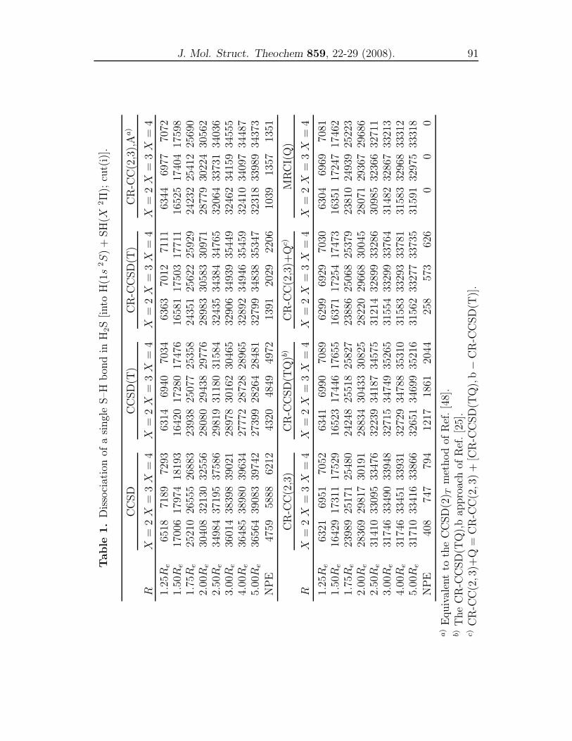
J. Mol. Struct. Theochem 859, 22-29 (2008). 91
Table
1.
Dis
soci
atio
nof
asi
ngl
eS
–Hb
ond
inH
2S
[into
H(1s
2S
)+
SH
(X2Π
);cu
t(i)
].
CC
SD
CC
SD
(T)
CR
-CC
SD
(T)
CR
-CC
(2,3
),A
a)
RX
=2X
=3X
=4
X=
2X
=3X
=4
X=
2X
=3X
=4
X=
2X
=3X
=4
1.25R
e65
1871
8972
9363
1469
4070
3463
6370
1271
1163
4469
7770
721.
50R
e17
006
1797
418
193
1642
017
280
1747
616
581
1750
317
711
1652
517
404
1759
81.
75R
e25
210
2655
526
883
2393
825
077
2535
824
351
2562
225
929
2423
225
412
2569
02.
00R
e30
408
3213
032
556
2808
029
438
2977
628
983
3058
330
971
2877
930
224
3056
22.
50R
e34
984
3719
537
586
2981
931
180
3158
432
435
3438
434
765
3206
433
731
3403
63.
00R
e36
014
3839
839
021
2897
830
162
3046
532
906
3493
935
449
3246
234
159
3455
54.
00R
e36
485
3898
039
634
2777
228
728
2896
532
892
3494
635
459
3241
034
097
3448
75.
00R
e36
564
3908
339
742
2739
928
264
2848
132
799
3483
835
347
3231
833
989
3437
3
NP
E47
5958
8862
1243
2048
4949
7213
9120
2922
0610
3913
5713
51
CR
-CC
(2,3
)C
R-C
CS
D(T
Q)b)
CR
-CC
(2,3
)+Q
c)M
RC
I(Q
)
RX
=2X
=3X
=4
X=
2X
=3X
=4
X=
2X
=3X
=4
X=
2X
=3X
=4
1.25R
e63
2169
5170
5263
4169
9070
8962
9969
2970
3063
0469
6970
811.
50R
e16
429
1731
117
529
1652
317
446
1765
516
371
1725
417
473
1635
117
247
1746
21.
75R
e23
989
2517
125
480
2424
825
518
2582
723
886
2506
825
379
2381
024
939
2522
32.
00R
e28
369
2981
730
191
2883
430
433
3082
528
220
2966
830
045
2807
129
367
2968
62.
50R
e31
410
3309
533
476
3223
934
187
3457
531
214
3289
933
286
3098
532
366
3271
13.
00R
e31
746
3349
033
948
3271
534
749
3526
531
554
3329
933
764
3148
232
867
3321
34.
00R
e31
746
3345
133
931
3272
934
788
3531
031
583
3329
333
781
3158
332
968
3331
25.
00R
e31
710
3341
633
866
3265
134
699
3521
631
562
3327
733
735
3159
132
975
3331
8
NP
E40
874
779
412
1718
6120
4425
857
362
60
00
a)
Equ
ival
ent
toth
eC
CS
D(2
) Tm
eth
od
ofR
ef.
[48]
.b)
Th
eC
R-C
CS
D(T
Q),
bap
pro
ach
ofR
ef.
[25]
.c)
CR
-CC
(2,3
)+Q
=C
R-C
C(2,3
)+
[CR
-CC
SD
(TQ
),b−
CR
-CC
SD
(T)]
.
92 Y. Z. Song, A. Kinal, P.J.S.B. Caridade, P. Piecuch and A.J.C. Varandas
produces errors relative to MRCI(Q) that monotonically increase with the S–H
distance R. The most accurate non-iterative treatment of triply excited clusters
offered by the CR-CC(2,3) approach is sufficient in this case to produce a highly
accurate description. Indeed, the CR-CC(2,3) method reduces the 4,973, 6108,
and 6,424 cm−1 maximum errors in the CCSD/X= 2−4 results for cut (i), relative
to MRCI(Q), to 425, 729, and 765 cm−1, respectively (see Table 1 and Figure 1).
The CR-CC(2,3)+Q approach reduces these maximum errors even further, to 229,
533, and 575 cm−1, respectively. These are impressive improvements if we realize
the serious difficulties the traditional CC approaches, such as CCSD(T), have in
describing the PES of H2S, and the fact that the energies characterizing cut (i)
exceed 30, 000 cm−1 as the S–H bond is significantly stretched. The differences
between the CR-CC(2,3) or CR-CC(2,3)+Q and MRCI(Q) energies on the order
of a few hundred cm−1 at larger S–H separations are within the accuracy of the
MRCI(Q) calculation, so that we can regard the CR-CC(2,3), CR-CC(2,3)+Q,
and MRCI(Q) results as essentially equivalent. This is emphasized by the small
non-parallelity errors (NPEs) relative to MRCI(Q) characterizing the CR-CC(2,3)
and CR-CC(2,3)+Q data in Table 1 (NPE is defined as the difference between
the maximum and minimum signed errors relative to MRCI(Q) along a PES cut).
The situation created by cut (ii) is entirely different and more challenging.
In this case, the CCSD approach is no longer qualitatively correct, producing a
large, unphysical hump in the region of the intermediate R values. This can be
understood if we realize that cut (ii) corresponds to a double S–H dissociation,
which is, in a zero-order description, a four-electron process that requires the
explicit inclusion of the triply as well as quadruply excited clusters. The proper
treatment of these clusters offered by the CR-CC(2,3)+Q method leads to a
highly accurate description of cut (ii), which can compete with the MRCI(Q)
results (see Table 2 and Figure 1). For example, the CR-CC(2,3)+Q approach
reduces the 5989 and 8402 cm−1 errors relative to MRCI(Q) in the CCSD results
at R = 2Re and R = 3Re obtained with the X = 4 basis set, where the MRCI(Q)
energies become as high as 58,056 and 63,560 cm−1, respectively, to as little as 580
and 684 cm−1, while providing a smooth description of cut (ii), with the energies
monotonically increasing R. The relative small NPE values relative to MRCI(Q)
characterizing the CR-CC(2,3)+Q results, which range, depending on the basis
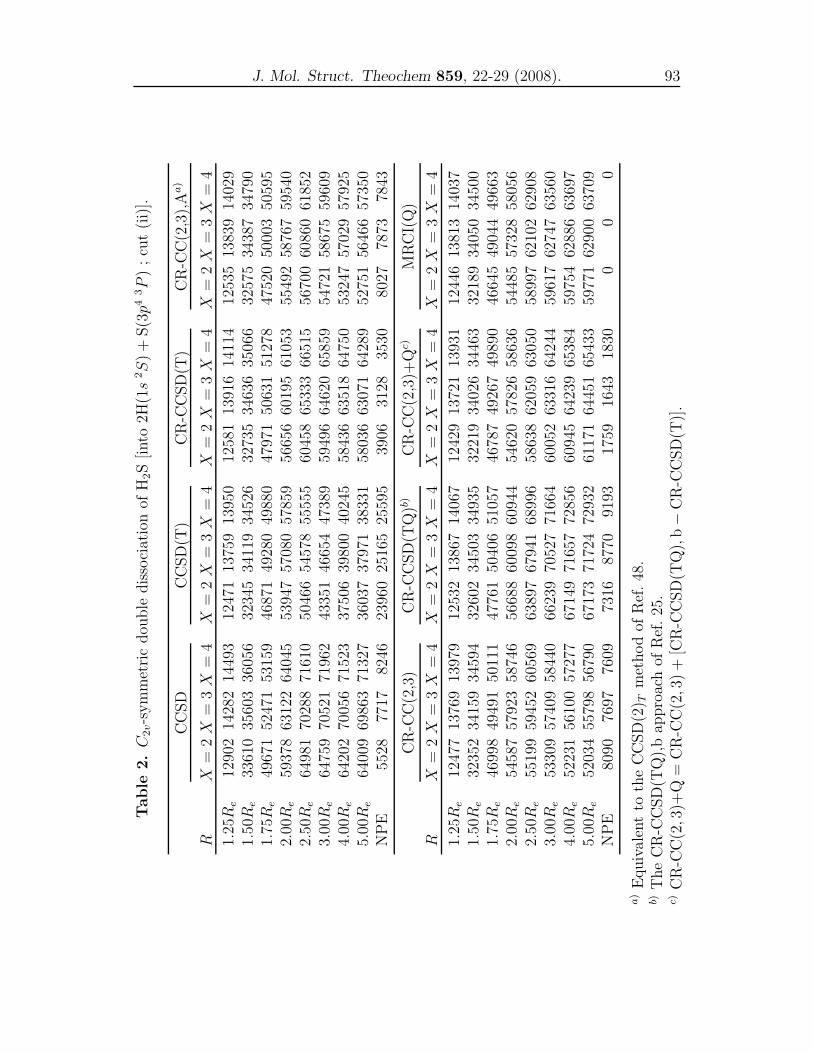
J. Mol. Struct. Theochem 859, 22-29 (2008). 93
Table
2.C
2v-s
ym
met
ric
dou
ble
dis
soci
atio
nof
H2S
[into
2H(1s
2S
)+
S(3p4
3P
);
cut
(ii)
].
CC
SD
CC
SD
(T)
CR
-CC
SD
(T)
CR
-CC
(2,3
),A
a)
RX
=2X
=3X
=4
X=
2X
=3X
=4
X=
2X
=3X
=4
X=
2X
=3X
=4
1.25R
e12
902
1428
214
493
1247
113
759
1395
012
581
1391
614
114
1253
513
839
1402
91.
50R
e33
610
3560
336
056
3234
534
119
3452
632
735
3463
635
066
3257
534
387
3479
01.
75R
e49
671
5247
153
159
4687
149
280
4988
047
971
5063
151
278
4752
050
003
5059
52.
00R
e59
378
6312
264
045
5394
757
080
5785
956
656
6019
561
053
5549
258
767
5954
02.
50R
e64
981
7028
871
610
5046
654
578
5555
560
458
6533
366
515
5670
060
860
6185
23.
00R
e64
759
7052
171
962
4335
146
654
4738
959
496
6462
065
859
5472
158
675
5960
94.
00R
e64
202
7005
671
523
3750
639
800
4024
558
436
6351
864
750
5324
757
029
5792
55.
00R
e64
009
6986
371
327
3603
737
971
3833
158
036
6307
164
289
5275
156
466
5735
0N
PE
5528
7717
8246
2396
025
165
2559
539
0631
2835
3080
2778
7378
43
CR
-CC
(2,3
)C
R-C
CS
D(T
Q)b)
CR
-CC
(2,3
)+Q
c)M
RC
I(Q
)
RX
=2X
=3X
=4
X=
2X
=3X
=4
X=
2X
=3X
=4
X=
2X
=3X
=4
1.25R
e12
477
1376
913
979
1253
213
867
1406
712
429
1372
113
931
1244
613
813
1403
71.
50R
e32
352
3415
934
594
3260
234
503
3493
532
219
3402
634
463
3218
934
050
3450
01.
75R
e46
998
4949
150
111
4776
150
406
5105
746
787
4926
749
890
4664
549
044
4966
32.
00R
e54
587
5792
358
746
5668
860
098
6094
454
620
5782
658
636
5448
557
328
5805
62.
50R
e55
199
5945
260
569
6389
767
941
6899
658
638
6205
963
050
5899
762
102
6290
83.
00R
e53
309
5740
958
440
6623
970
527
7166
460
052
6331
664
244
5961
762
747
6356
04.
00R
e52
231
5610
057
277
6714
971
657
7285
660
945
6423
965
384
5975
462
886
6369
75.
00R
e52
034
5579
856
790
6717
371
724
7293
261
171
6445
165
433
5977
162
900
6370
9N
PE
8090
7697
7609
7316
8770
9193
1759
1643
1830
00
0
a)
Equ
ival
ent
toth
eC
CS
D(2
) Tm
eth
od
ofR
ef.
48.
b)T
he
CR
-CC
SD
(TQ
),b
app
roac
hof
Ref
.25
.c)
CR
-CC
(2,3
)+Q
=C
R-C
C(2,3
)+
[CR
-CC
SD
(TQ
),b−
CR
-CC
SD
(T)]
.
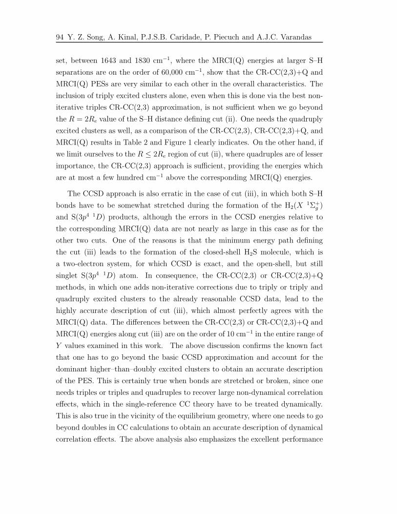
94 Y. Z. Song, A. Kinal, P.J.S.B. Caridade, P. Piecuch and A.J.C. Varandas
set, between 1643 and 1830 cm−1, where the MRCI(Q) energies at larger S–H
separations are on the order of 60,000 cm−1, show that the CR-CC(2,3)+Q and
MRCI(Q) PESs are very similar to each other in the overall characteristics. The
inclusion of triply excited clusters alone, even when this is done via the best non-
iterative triples CR-CC(2,3) approximation, is not sufficient when we go beyond
the R = 2Re value of the S–H distance defining cut (ii). One needs the quadruply
excited clusters as well, as a comparison of the CR-CC(2,3), CR-CC(2,3)+Q, and
MRCI(Q) results in Table 2 and Figure 1 clearly indicates. On the other hand, if
we limit ourselves to the R ≤ 2Re region of cut (ii), where quadruples are of lesser
importance, the CR-CC(2,3) approach is sufficient, providing the energies which
are at most a few hundred cm−1 above the corresponding MRCI(Q) energies.
The CCSD approach is also erratic in the case of cut (iii), in which both S–H
bonds have to be somewhat stretched during the formation of the H2(X1Σ+
g )
and S(3p4 1D) products, although the errors in the CCSD energies relative to
the corresponding MRCI(Q) data are not nearly as large in this case as for the
other two cuts. One of the reasons is that the minimum energy path defining
the cut (iii) leads to the formation of the closed-shell H2S molecule, which is
a two-electron system, for which CCSD is exact, and the open-shell, but still
singlet S(3p4 1D) atom. In consequence, the CR-CC(2,3) or CR-CC(2,3)+Q
methods, in which one adds non-iterative corrections due to triply or triply and
quadruply excited clusters to the already reasonable CCSD data, lead to the
highly accurate description of cut (iii), which almost perfectly agrees with the
MRCI(Q) data. The differences between the CR-CC(2,3) or CR-CC(2,3)+Q and
MRCI(Q) energies along cut (iii) are on the order of 10 cm−1 in the entire range of
Y values examined in this work. The above discussion confirms the known fact
that one has to go beyond the basic CCSD approximation and account for the
dominant higher–than–doubly excited clusters to obtain an accurate description
of the PES. This is certainly true when bonds are stretched or broken, since one
needs triples or triples and quadruples to recover large non-dynamical correlation
effects, which in the single-reference CC theory have to be treated dynamically.
This is also true in the vicinity of the equilibrium geometry, where one needs to go
beyond doubles in CC calculations to obtain an accurate description of dynamical
correlation effects. The above analysis also emphasizes the excellent performance
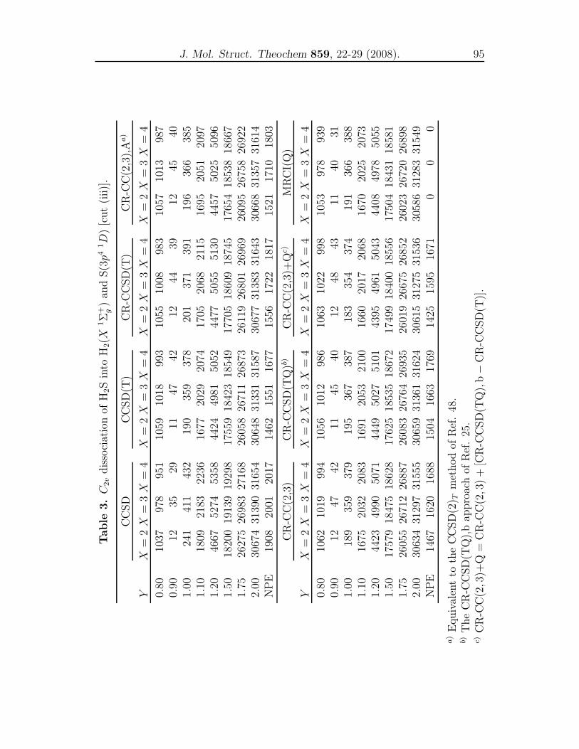
J. Mol. Struct. Theochem 859, 22-29 (2008). 95
Table
3.C
2v
dis
soci
atio
nof
H2S
into
H2(X
1Σ
+ g)
and
S(3p4
1D
)[c
ut
(iii
)].
CC
SD
CC
SD
(T)
CR
-CC
SD
(T)
CR
-CC
(2,3
),A
a)
YX
=2X
=3X
=4
X=
2X
=3X
=4
X=
2X
=3X
=4
X=
2X
=3X
=4
0.80
1037
978
951
1059
1018
993
1055
1008
983
1057
1013
987
0.90
1235
2911
4742
1244
3912
4540
1.00
241
411
432
190
359
378
201
371
391
196
366
385
1.10
1809
2183
2236
1677
2029
2074
1705
2068
2115
1695
2051
2097
1.20
4667
5274
5358
4424
4981
5052
4477
5055
5130
4457
5025
5096
1.50
1820
019
139
1929
817
559
1842
318
549
1770
518
609
1874
517
654
1853
818
667
1.75
2627
526
983
2716
826
058
2671
126
873
2611
926
801
2696
926
095
2675
826
922
2.00
3067
431
390
3165
430
648
3133
131
587
3067
731
383
3164
330
668
3135
731
614
NP
E19
0820
0120
1714
6215
5116
7715
5617
2218
1715
2117
1018
03
CR
-CC
(2,3
)C
R-C
CS
D(T
Q)b)
CR
-CC
(2,3
)+Q
c)M
RC
I(Q
)
YX
=2X
=3X
=4
X=
2X
=3X
=4
X=
2X
=3X
=4
X=
2X
=3X
=4
0.80
1062
1019
994
1056
1012
986
1063
1022
998
1053
978
939
0.90
1247
4211
4540
1248
4311
4031
1.00
189
359
379
195
367
387
183
354
374
191
366
388
1.10
1675
2032
2083
1691
2053
2100
1660
2017
2068
1670
2025
2073
1.20
4423
4990
5071
4449
5027
5101
4395
4961
5043
4408
4978
5055
1.50
1757
918
475
1862
817
625
1853
518
672
1749
918
400
1855
617
504
1843
118
581
1.75
2605
526
712
2688
726
083
2676
426
935
2601
926
675
2685
226
023
2672
026
898
2.00
3063
431
297
3155
530
659
3136
131
624
3061
531
275
3153
630
586
3128
331
549
NP
E14
6716
2016
8815
0416
6317
6914
2515
9516
710
00
a)
Equ
ival
ent
toth
eC
CS
D(2
) Tm
eth
od
ofR
ef.
48.
b)T
he
CR
-CC
SD
(TQ
),b
app
roac
hof
Ref
.25
.c)
CR
-CC
(2,3
)+Q
=C
R-C
C(2,3
)+
[CR
-CC
SD
(TQ
),b−
CR
-CC
SD
(T)]
.
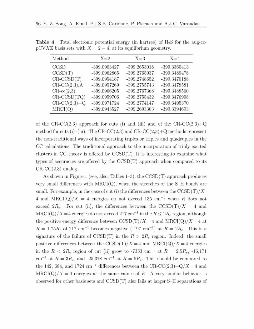
96 Y. Z. Song, A. Kinal, P.J.S.B. Caridade, P. Piecuch and A.J.C. Varandas
Table 4. Total electronic potential energy (in hartree) of H2S for the aug-cc-pCVXZ basis sets with X = 2 − 4, at its equilibrium geometry.
Method X=2 X=3 X=4
CCSD -399.0903427 -399.2653018 -399.3360413CCSD(T) -399.0962865 -399.2765937 -399.3489478CR-CCSD(T) -399.0954187 -399.2748652 -399.3470188CR-CC(2,3),A -399.0957269 -399.2755743 -399.3478581CR-cc(2,3) -399.0966205 -399.2767368 -399.3488560CR-CCSD(TQ) -399.0959706 -399.2755432 -399.3476998CR-CC(2,3)+Q -399.0971724 -399.2774147 -399.3495370MRCI(Q) -399.0943527 -399.2693303 -399.3394693
of the CR-CC(2,3) approach for cuts (i) and (iii) and of the CR-CC(2,3)+Q
method for cuts (i)–(iii). The CR-CC(2,3) and CR-CC(2,3)+Q methods represent
the non-traditional ways of incorporating triples or triples and quadruples in the
CC calculations. The traditional approach to the incorporation of triply excited
clusters in CC theory is offered by CCSD(T). It is interesting to examine what
types of accuracies are offered by the CCSD(T) approach when compared to its
CR-CC(2,3) analog.
As shown in Figure 1 (see, also, Tables 1–3), the CCSD(T) approach produces
very small differences with MRCI(Q), when the stretches of the S–H bonds are
small. For example, in the case of cut (i) the differences between the CCSD(T)/X=
4 and MRCI(Q)/X = 4 energies do not exceed 135 cm−1 when R does not
exceed 2Re. For cut (ii), the differences between the CCSD(T)/X = 4 and
MRCI(Q)/X=4 energies do not exceed 217 cm−1 in the R ≤ 2Re region, although
the positive energy difference between CCSD(T)/X = 4 and MRCI(Q)/X = 4 at
R = 1.75Re of 217 cm−1 becomes negative (-197 cm−1) at R = 2Re. This is a
signature of the failure of CCSD(T) in the R > 2Re region. Indeed, the small
positive differences between the CCSD(T)/X = 4 and MRCI(Q)/X = 4 energies
in the R < 2Re region of cut (ii) grow to -7353 cm−1 at R = 2.5Re, -16,171
cm−1 at R = 3Re, and -25,378 cm−1 at R = 5Re. This should be compared to
the 142, 684, and 1724 cm−1 differences between the CR-CC(2,3)+Q/X=4 and
MRCI(Q)/X = 4 energies at the same values of R. A very similar behavior is
observed for other basis sets and CCSD(T) also fails at larger S–H separations of
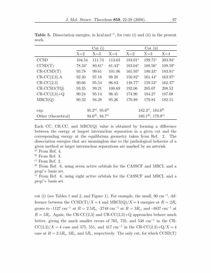
J. Mol. Struct. Theochem 859, 22-29 (2008). 97
Table 5. Dissociation energies, in kcal mol−1, for cuts (i) and (ii) in the presentwork.
Cut (i) Cut (ii)
X=2 X=3 X=4 X=2 X=3 X=4
CCSD 104.54 111.74 113.63 183.01∗ 199.75∗ 203.94∗
CCSD(T) 78.34∗ 80.81∗ 81.43∗ 103.04∗ 108.56∗ 109.59∗
CR-CCSD(T) 93.78 99.61 101.06 165.93∗ 180.33∗ 183.81∗
CR-CC(2,3),A 92.40 97.18 98.28 150.82∗ 161.44∗ 163.97∗
CR-CC(2,3) 90.66 95.54 96.83 148.77∗ 159.53∗ 162.37∗
CR-CCSD(TQ) 93.35 99.21 100.69 192.06 205.07 208.52
CR-CC(2,3)+Q 90.24 95.14 96.45 174.90 184.27 187.08
MRCI(Q) 90.32 94.28 95.26 170.89 179.84 182.15
exp. 95.2a), 95.6b) 182.3c), 184.6b)
Other (theoretical) 94.6d), 94.7e) 180.1d), 179.8e)
Each CC, CR-CC, and MRCI(Q) value is obtained by forming a differencebetween the energy at largest internuclear separation in a given cut and thecorresponding energy at the equilibrium geometry taken from Ref. 2. Thedissociation energies that are meaningless due to the pathological behavior of agiven method at larger internuclear separations are marked by an asterisk.a) From Ref. 4.b) From Ref. 3.c) From Ref. 2.d) From Ref. 6, using seven active orbitals for the CASSCF and MRCI, and apvqz′+ basis set.e) From Ref. 6, using eight active orbitals for the CASSCF and MRCI, and apvqz′+ basis set.
cut (i) (see Tables 1 and 2, and Figure 1). For example, the small, 90 cm−1, dif-
ference between the CCSD(T)/X = 4 and MRCI(Q)/X = 4 energies at R = 2Re
grows to -1127 cm−1 at R = 2.5Re, -2748 cm−1 at R = 3Re, and -4837 cm−1 at
R = 5Re. Again, the CR-CC(2,3) and CR-CC(2,3)+Q approaches behave much
better, giving the much smaller errors of 765, 735, and 548 cm−1 in the CR-
CC(2,3)/X = 4 case and 575, 551, and 417 cm−1 in the CR-CC(2,3)+Q/X = 4
case at R = 2.5Re, 3Re, and 5Re, respectively. The only cut, for which CCSD(T)
98 Y. Z. Song, A. Kinal, P.J.S.B. Caridade, P. Piecuch and A.J.C. Varandas
works well, is cut (iii), where, in analogy to CR-CC(2,3), the differences between
the CCSD(T) and MRCI(Q) energies are on the order of 10 cm−1 in the entire
Y = 0.8 − 2.0 A region.
The approximate variant of CR-CC(2,3), termed CR-CC(2,3),A, which, as
stated earlier, is equivalent to the CCSD(2)T method of Ref. [48], and the CR-
CCSD(T) approach of Refs. [23–25], which also aim at improving the CCSD(T)
results are larger internuclear separations via non-iterative corrections due to
triples added to the CCSD energy, are not as effective as the full CR-CC(2,3)
method. Similarly, the CR-CC(2,3)+Q approach is more effective than the orig-
inal CR-CCSD(TQ),b method of Ref. [25]. For example, in the case of cut (i)
the relatively small errors in the CR-CC(2,3)/X=4 energies relative to the cor-
responding MRCI(Q)/X = 4 energies at R = 2Re, 3Re, and 5Re of 505, 735,
and 548 cm−1, respectively, are considerably smaller than the analogous errors
obtained with the CR-CC(2,3),A and CR-CCSD(T) approaches, which give 876,
1342, and 1055 cm−1 in the CR-CC(2,3),A case and 1285, 2236, and 2029 cm−1
in the CR-CCSD(T) case. The 2888, 8104, and 9223 cm−1 errors relative to
MRCI(Q) obtained with CR-CCSD(TQ)/X = 4 [i.e., CR-CCSD(TQ),b/X = 4]
method at R = 2Re, 3Re, and 5Re for cut (ii) reduce to 580, 684, and 1724 cm−1,
respectively, when the CR-CC(2,3)+Q/X = 4 method is employed (see Tables 1
and 2, and Figure 1). Similar improvements in the CR-CCSD(T), CR-CC(2,3),A,
and CR-CCSD(TQ) results offered by the CR-CC(2,3) and CR-CC(2,3)+Q ap-
proaches are observed for other basis sets. The CR-CCSD(T), CR-CC(2,3),A,
and CR-CCSD(TQ) methods improve the poor description of cuts (i) and (ii) in
regions of larger S–H distances by the CCSD(T) approach, but they are not as
effective as the CR-CC(2,3) and CR-CC(2,3)+Q approximations, The only cut
where the CR-CCSD(T), CR-CC(2,3),A, and CR-CCSD(TQ) methods are more
or less as effective as the CR-CC(2,3) and CR-CC(2,3)+Q approaches is cut (iii),
although even in that case the CR-CC(2,3) and CR-CC(2,3)+Q methods are
somewhat more accurate.
4 Summary and concluding remarks
We have compared the results of the conventional CCSD and CCSD(T), and
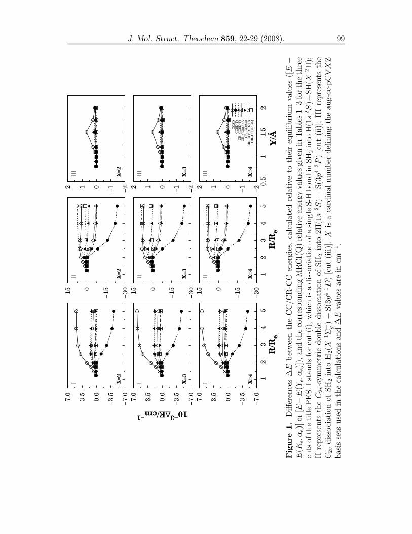
J. Mol. Struct. Theochem 859, 22-29 (2008). 99
−7
.0
−3
.5
0.0
3.5
7.0
1 2
3 4
5
R/R
e
X=4
Ι
−7
.0
−3
.5
0.0
3.5
7.0
10−3
∆E/cm−1
X=3
Ι
−7
.0
−3
.5
0.0
3.5
7.0
X=2
Ι
−3
0
−1
50
15
12
34
5
R/R
e
X=4
ΙΙ
−3
0
−1
50
15
X=3
ΙΙ
−3
0
−1
50
15
X=2
ΙΙ
−2
−1012 0
.51
1.5
2
Y/Å
X=4
ΙΙΙ
CC
SD
CC
SD
(T)
CR
−C
CS
D(T
)C
R−
CC
(2,3
),A
CR
−C
C(2
,3)
CR
−C
CS
D(T
Q),
BC
R−
CC
(2,3
)+Q
−2
−1012
X=3
ΙΙΙ
−2
−1012
X=2
ΙΙΙ
Fig
ure
1.
Diff
eren
ces
∆E
bet
wee
nth
eC
C/C
R-C
Cen
ergi
es,
calc
ula
ted
rela
tive
toth
eir
equ
ilib
riu
mva
lues
([E
−E
(Re,α
e)]
or[E
−E
(Ye,α
e)]
),an
dth
eco
rres
pon
din
gM
RC
I(Q
)re
lati
veen
ergy
valu
esgi
ven
inT
able
s1–
3fo
rth
eth
ree
cuts
ofth
eti
tle
PE
S.
Ist
and
sfo
rcu
t(i
),w
hic
his
ad
isso
ciat
ion
ofa
sin
gle
S-H
bon
din
SH
2in
toH
(1s
2S
)+S
H(X
2Π
);II
rep
rese
nts
theC
2v-s
ym
met
ric
dou
ble
dis
soci
atio
nof
SH
2in
to2H
(1s
2S
)+
S(3p4
3P
)[c
ut
(ii)
];II
Ire
pre
sents
the
C2v
dis
soci
atio
nof
SH
2in
toH
2(X
1Σ
+ g)
+S
(3p4
1D
)[c
ut
(iii
)].X
isa
card
inal
nu
mb
erd
efin
ing
the
aug-
cc-p
CVX
Zb
asis
sets
use
din
the
calc
ula
tion
san
d∆E
valu
esar
ein
cm−
1.
100Y. Z. Song, A. Kinal, P.J.S.B. Caridade, P. Piecuch and A.J.C. Varandas
the renormalized renormalized CR-CCSD(T), CR-CCSD(TQ), CR-CC(2,3), and
CR-CC(2,3)+Q calculations with the MRCI(Q) results for the three important
cuts of the H2S(1A′) PES, including the dissociation of a single S–H bond, which
correlates with the H(1s 2S) + SH(X 2Π) asymptote, the simultaneous dissoci-
ation of both S–H bonds, which leads to the 2H(1s 2S) + S(3p4 3P ) products,
and the C2v-symmetric minimum energy dissociation path into H2(X1Σ+
g ) and
S(3p4 1D). We have found that all renormalized CC methods reduce the failures
of the conventional CCSD and CCSD(T) approaches in the bond stretching re-
gions of the H2S potential, with the CR-CC(2,3) and CR-CC(2,3)+Q methods
being most effective in this regard. The size extensive CR-CC(2,3) method em-
ploying the standard RHF reference provides the results of the MRCI(Q) quality
for the dissociation of a single S–H bond and for the C2v-symmetric dissocia-
tion of H2S into H2(X 1Σ+g ) + S(3p4 1D). The CR-CC(2,3) approach corrected
for the effect of quadruply excited clusters via the CR-CC(2,3)+Q method im-
proves these results even further, while producing a highly accurate description
of the simultaneous dissociation of both S–H bonds that can compete with the
high-quality data obtained in the CASSCF-based MRCI(Q) calculations. At the
same time, the CR-CC(2,3) approach is as accurate as CCSD(T) in the equi-
librium region, with CR-CC(2,3)+Q providing additional small improvements.
The fact that the CR-CC(2,3)+Q approach works well in the outer regions of the
challenging cut (ii) is most encouraging, since it is difficult to obtain reliable in-
formation about the energetics of such regions, particularly with single-reference
methods. In the PES regions relevant to reaction dynamical applications, where
the outer part of path (ii) is energetically not accessible, the relative performance
of CR-CC(2,3)+Q is even better.
Acknowledgments
This work has the supported of Fundacao para a Ciencia e Tecnologia, Portugal,
and the U.S. Department of Energy.
J. Mol. Struct. Theochem 859, 22-29 (2008). 101
References
[1] S.-H. Lee and K. Liu, Chem. Phys. Lett. 290, 323 (1998).
[2] M. W. Chase Jr., C. A. Davies, J. R. Downey Jr., D. J. Frurip, R. A. McDon-
ald, and A. N. Syveraud, JANAF Thermodynamic Tables, 3rd. ed. (Amer-
ican Chemical Society and American Institute for Physics for the National
Bureau of Standards, New York, 1985).
[3] J. D. Cox, D. D. Wagmann, and V. A. Medvedev, CODATA Keyvalues for
Thermodynamic (Hemispher, New York, 1984).
[4] X. Xie, H. Wallmeier, R. Boettner, K. H. Welge, and M. N. R. Ashfold, J.
Phys. Chem. 92, 1608 (1990).
[5] S.-H. Lee and K. Liu, Appl. Phys. B 71, 627 (2000).
[6] A. S. Zyubin, A. M. Mebel, S. D. Chao, and R. T. Skodje, J. Chem. Phys.
114, 320 (2001).
[7] T.-S. Ho, T. Hollebeek, H. Rabitz, S. D. Chao, R. T. Skodje, A. S. Zyubin,
and A. M. Mebel, J. Chem. Phys. 116, 4124 (2002).
[8] B. Maiti, G. C. Schatz, and G. Lendvay, J. Phys. Chem. A 108, 8772 (2004).
[9] S. D. Chao and R. T. Skodje, J. Phys. Chem. A 105, 2474 (2001).
[10] H. Shiina, A. Miyoshi, and H. Matsui, J. Phys. Chem. A 102, 3556 (1998).
[11] T. H. Dunning Jr., J. Chem. Phys. 90, 1007 (1989).
[12] D. E. Woon and T. H. Dunning Jr., J. Chem. Phys. 98, 1358 (1993).
[13] P. Piecuch, S. A. Kucharski, K. Kowalski, and M. Musia l, Comp. Phys.
Comm. 149, 71 (2002).
[14] P. Piecuch and M. W loch, J. Chem. Phys. 123, 224105 (2005).
[15] M. W. Schmidt, K. K. Baldridge, J. A. Boatz, S. T. Elbert, M. S. Gordon,
J. H. Jensen, S. Koseki, N. Matsunaga, K. A. Nguyen, S. J. Su, T. L. Windus,
M. Dupuis, and J. A. Montgomery, Jr., J. Comput. Chem. 14, 1347 (1993).
102Y. Z. Song, A. Kinal, P.J.S.B. Caridade, P. Piecuch and A.J.C. Varandas
[16] H.-J. Werner and P. J. Knowles, J. Chem. Phys. 89, 5803 (1988).
[17] P. J. Knowles and H.-J. Werner, Chem. Phys. Lett. 145, 514 (1988).
[18] H.-J. Werner et al.,MOLPRO, version 2002.6;a package of ab initio programs;
Available from: http://www.molpro.net (Birmingham, UK, 2003).
[19] G. D. Purvis III and R. J. Bartlett, J. Chem. Phys. 76, 1910 (1982).
[20] G. E. Scuseria, A. C. Scheiner, T. J. Lee, J. E. Rice, and H. F. Schaefer III,
J. Chem. Phys. 86, 2881 (1987).
[21] P. Piecuch and J. Paldus, Int. J. Quantum Chem. 36, 429 (1989).
[22] K. Raghavachari, G. W. Trucks, J. A. Pople, and M. H. Gordon, Chem.
Phys. Lett. 157, 479 (1989).
[23] P. Piecuch and K. Kowalski, in: Computational Chemistry: Reviews of Cur-
rent Trends, edited by J. Leszczynski (World Scientific, Singapore, 2000),
Vol. 5, pp. 1-104.
[24] K. Kowalski and P. Piecuch, J. Chem. Phys. 113, 18 (2000).
[25] K. Kowalski and P. Piecuch, J. Chem. Phys. 113, 5644 (2000).
[26] P. Piecuch, M. W loch, J. R. Gour, and A. Kinal, Chem. Phys. Lett. 418,
467 (2005).
[27] M. W loch, M. D. Lodriguito, P. Piecuch, and J. R. Gour, Mol. Phys. 104,
2149 (2006).
[28] M. W loch, J. R. Gour, and P. Piecuch, J. Phys. Chem. A, submitted (2007).
[29] P. Piecuch, K. Kowalski, I. S. O. Pimienta, and M. J. McGuire, Int. Rev.
Phys. Chem. 21, 527 (2002).
[30] P. Piecuch, K. Kowalski, P.-D. Fan, and I. S. O. Pimienta, in: Progress in
Theoretical Chemistry and Physics, Vol. 12, Advanced Topics in Theoreti-
cal Chemical Physics, edited by J. Maruani, R. Lefebvre, and E. Brandas
(Kluwer, Dordrecht, 2003), pp. 119-206.
J. Mol. Struct. Theochem 859, 22-29 (2008). 103
[31] P. Piecuch, K. Kowalski, I. S. O. Pimienta, P.-D. Fan, M. Lodriguito, M. J.
McGuire, S. A. Kucharski, T. Kus, and M. Musia l, Theor. Chem. Acc. 112,
349 (2004).
[32] P. Piecuch, M. W loch, M. Lodriguito, and J. R. Gour, in: Progress in
Theoretical Chemistry and Physics, Vol. 15, Recent Advances in the The-
ory of Chemical and Physical Systems, edited by J.-P. Julien, J. Maruani,
D. Mayou, S. Wilson, and G. Delgado-Barrio (Springer, Berlin, 2006), pp.
45-106.
[33] P. Piecuch, M. W loch, and A. J. C. Varandas, in: Progress in Theoretical
Chemistry and Physics, Vol. 16, edited by S. Lahmar, J. Maruani, S. Wilson,
and G. Delgado-Barrio (Springer, Berlin, 2007), pp. 65-133.
[34] P. Piecuch, M. W loch, and A. J. C. Varandas, Theor. Chem. Acc., in press
(2007).
[35] C. J. Cramer, M. W loch, P. Piecuch, C. Puzzarini, and L. Gagliardi, J. Phys.
Chem. A 110, 1991 (2006).
[36] C. J. Cramer, A. Kinal, M. W loch, P. Piecuch, and L. Gagliardi, J. Phys.
Chem. A 110, 11557 (2006).
[37] Y. Ge, M. S. Gordon and P. Piecuch, J. Chem. Phys. 127, 10548 (2007).
[38] A. J. C. Varandas, J. Chem. Phys. 105, 3524 (1996).
[39] K. A. Peterson and T. H. Dunning Jr., J. Chem. Phys. 117, 10548 (2002).
[40] O. L. Polyansky, A. G. Csaszar, S. V. Shirin, N. F. Zobov, P. Bartletta, J.
Tennyson, D. W. Schwenke, and P. J. Knowles, Science 299, 539 (2003).
[41] E. F. Valeev, W. D. Allen, H. F. Schaefer III, and A. G. Csaszar, J. Chem.
Phys. 114, 2875 (2001).
[42] C. D. Sherrill and P. Piecuch, J. Chem. Phys. 122, 124104 (2005)

104Y. Z. Song, A. Kinal, P.J.S.B. Caridade, P. Piecuch and A.J.C. Varandas
[43] P. Piecuch, K. Kowalski, I. S. O. Pimienta, and S. A. Kucharski, in: Low-
Lying Potential Energy Surfaces, ACS Symposium Series, Vol. 828, edited by
M.R. Hoffmann and K.G. Dyall (American Chemican Society, Washington,
D.C., 2002), pp. 31-64.
[44] K. Kowalski and P. Piecuch, Chem. Phys. Lett. 344, 165 (2001).
[45] P. Piecuch, S. A. Kucharski, V. Spirko, and K. Kowalski, J. Chem. Phys.
115, 5796 (2001).
[46] M. J. McGuire, K. Kowalski, and P. Piecuch, J. Chem. Phys. 117, 3617
(2002).
[47] M. J. McGuire, K. Kowalski, P. Piecuch, S. A. Kucharski, and M. Musia l,
J. Phys. Chem. A 108, 8878 (2004).
[48] S. Hirata, P.-D. Fan, A. A. Auer, M. Nooijen, and P. Piecuch, J. Chem.
Phys. 121, 12197 (2004).
[49] K. Kowalski and P. Piecuch, J. Chem. Phys. 122, 074107 (2005).
[50] P. Piecuch, S. Hirata, K. Kowalski, P.-D. Fan, and T. L. Windus, Int. J.
Quantum Chem. 106, 79 (2006).
[51] M. J. McGuire and P. Piecuch, J. Am. Chem. Soc. 127, 2608 (2005).
[52] A. Kinal and P. Piecuch, J. Phys. Chem. A 110, 367 (2006).
[53] A. Kinal and P. Piecuch, J. Phys. Chem. A 111, 734 (2007).
[54] Basis sets were obtained from the Extensible Computational Chemistry Envi-
ronment Basis Set Database, Version 02/02/06, as developed and distributed
by the Molecular Science Computing Facility, Environmental and Molecu-
lar Sciences Laboratory which is part of the Pacific Northwest Laboratory,
P.O. Box 999, Richland, Washington 99352, USA, and funded by the U.S.
Department of Energy. The Pacific Northwest Laboratory is a multiprogram
laboratory operated by Battelle Memorial Institute for the U.S. Department
of Energy under contract DE-AC06-76RLO 1830. Contact Karen Schuchardt
for further information.
Chapter 5
Accurate DMBE/CBS PES forground-state H2S

J. Chem. Phys 130, 134317-134326 (2009).
Accurate ab initio double many-body expansionpotential energy surface for ground-state H2S byextrapolation to the complete basis set limit
Y. Z. Song and A.J.C. Varandas
Departamento de Quımica, Universidade de Coimbra
3004-535 Coimbra Codex, Portugal.
(Received: January 15, 2009; accepted: March 2, 2009)
Abstract
A single-sheeted potential energy surface is reported for the ground-state H2S by fit-
ting accurate multireference configuration interaction energies calculated using aug-cc-
pVTZ and aug-cc-pVQZ basis sets with extrapolation of the electron correlation energy
to the complete basis set limit, plus extrapolation to the complete basis set limit of
the complete-active-space self-consistent field energy. A switching function has been
used to warrant the correct behavior at the H2(X1Σ+
g )+S(1D) and SH(X 2Π)+H(2S)
dissociation limits. The topographical features of the novel global potential energy sur-
face are examined in details, with the former being used for exploratory quasi-classical
trajectory calculations of the thermal rate constants for the S(1D)+H2, S(1D)+D2,
and S(1D)+HD reactions at room temperature. A comparison with other available
potential energy surfaces as well as kinetics data is also provided.
108 Y.Z. Song and A.J.C. Varandas
1 Introduction
Recently, the research on the potential energy surface (PES) and dynamics of H2S
has been the subject of considerable experimental and theoretical work. Among
the many experiments that have been reported are those by Lee and Liu1, 2 who
employed a Doppler-selected time-of-flight technique in combination with crossed
molecular beam experiment to measure integral cross sections and vibrational
state-resolved differential cross sections in collisions of S(1D) with H2 reactions
at translational energies from 0.6 to 6 kcal/mol. Accurate equilibrium geometry
and local PES have also been explored by a large number of experiment studies.3–6
Theoretically, much research has been carried out on the PES and dynam-
ics for the reaction S(1D) + H2.7–13 In particular, Zyubin et al.7 studied the
dynamics of the S(1D) + H2/D2 reactions using an ab initio PES calculated at
the multi-reference configuration interaction14 (MRCI) level with a multiconfig-
uration self-consistent field (MCSCF) reference wave function and a number of
correlation-consistent basis sets,15, 16 including the simplified variant of the aug-
cc-pVQZ basis set (such basis are generally denoted as AVXZ, with X being
usually referred to as the basis-set cardinal number), commonly abbreviated as
pvqz′+. In turn, Ho et al.10 studied the S(1D) + H2 reaction using a PES ob-
tained by an improved interpolation of the MRCI data of Zyubin et al.7 on a
three-dimensional regular grid in Jacobi coordinates. Both calculations7, 10 indi-
cate a barrier-free insertion pathway along T-shaped geometries. Recently, we
also obtained a quite reliable global PES for H2S(1A′)13 based on double many-
body expansion (DMBE) 17–19 theory, which is calibrated using 1972 MRCI points
based on the full valence complete active space (FVCAS) (Ref. 20) reference func-
tion and the AVQZ15, 21 basis set. As usual in our group, the MRCI energies cal-
culated in this way have been subsequently corrected semiempirically using the
double many-body expansion-scaled external correlation (DMBE-SEC) (Ref. 22)
method to mimic the complete basis set plus full configuration interaction limit.
The PES so obtained (hereinafter referred to as DMBE/SEC) shows the correct
long range behavior and provides a realistic representation of the PES features
at all interatomic separations.
However, the PESs mentioned above depend on the one-electron basis set

J. Chem. Phys 130, 134317-134326 (2009). 109
used for the calculation or contain some empiricism. To obtain a high-accuracy
PES using only conventional ab initio calculations, one must extrapolate to the
one-electron complete basis set (CBS) limit.23–25 Much effort has been put to
devise efficient, yet simple, extrapolation schemes.26–34 In particular, Varandas31
suggested a dual-level approach referred to as uniform singlet- and triplet-pair
extrapolation (USTE) protocol, which has been now amply tested. In particular,
the USTE scheme has been shown to extrapolate the full correlation energies
for seven closed-shell systems CH2(1A1), H2O, HF, N2, CO, Ne, and F2 at their
equilibrium geometries with a similar, often better, accordance with the target
results than the traditional and rather successful Klopper’s extrapolations pro-
tocol.28 It has also been shown35 to compare favorably with the akin numeri-
cal scheme devised by Schwenke.36 Such good performance in comparison with
the best estimates of the extrapolated energies has been observed even when
the extrapolation employs a pair of correlation-consistent basis sets with cardi-
nal numbers as low as (D, T ).37 Of particular relevance for the present work is
Varandas’ extrapolation32 of the potential energy curve of CO(A 1Π) where an
excellent agreement with experiment is obtained, especially for the minimum well
depth and location of equilibrium CO. We follow here a similar route, with our
results corroborating the findings reported in Ref. 32, which suggest that our
strategy33, 38, 39 can provide a general approach for accurate potentials of larger
dimensionality at costs that can be drastically smaller than the traditional ones.
The major goal of the current work is therefore to obtain a high quality PES of
H2S(X 1A′) via extrapolation of the electron correlation energy to the CBS limit
plus extrapolation to the CBS limit of the complete-active-space self-consistent
field energy. For this, we employ a generalization31, 32 of the scheme proposed by
Karton and Martin30 for the Hartree-Fock energies, while the dynamical correla-
tion is extrapolated using the USTE (Ref. 31) protocol. This will be done using
two relatively inexpensive basis sets for the title system, namely, the AVTZ and
AVQZ ones, although as noted above the approach has shown to yield promising
results even when employing more modest correlation consistent basis sets.
The paper is organized as follows. Section 2 describes the ab initio calculations
carried out in the present work, while the extrapolation procedure is described
in Section 3. The analytical modeling of the PES is presented in Section 4.
110 Y.Z. Song and A.J.C. Varandas
Specifically, Section 4.1 focuses on the switching function formalism, Section 4.2
on the two-body energy terms, Section 4.3 on the three-body ones. The main
topographical features of the DMBE/CBS PES are discussed in Section 5. In
Section 6, a comparison of the quasiclassical trajectory (QCT) calculations for
the S(1D)+H2 thermal rate constant and its various isotopomers at T = 300 K
with the experimental and the other theoretical results is also given. Section 7
gathers the concluding remarks.
2 Ab initio calculations
All electronic structure calculations have been carried out at the MRCI (Ref. 14)
[including the popular quasidegenerate Davidson correction, MRCI(Q)] level us-
ing the FVCAS (Ref. 20) wave function as reference. The aug-cc-pVTZ (AVTZ)
and aug-cc-pVQZ (AVQZ) basis sets of Dunning15, 21 have been employed40 and
the calculations carried out using the MOLPRO (Ref. 41) package. The core
orbitals have been kept frozen in all calculations, with the result of this being
briefly commented later. A total of 1984 grid points have been chosen to map the
PES over the S−H2 region defined by 1.4 ≤ RH2/a0 ≤ 3.4, 1.0 ≤ rS−H2
/a0 ≤ 10.0
and 0.0 ≤ γ/ deg ≤ 90. For the H − SH interactions, a grid defined by 2.0 ≤RSH/a0 ≤ 3.6, 1.0 ≤ rH−SH/a0 ≤ 10.0 and 0.0 ≤ γ/deg ≤ 180 has been chosen.
For both channels, r, R and γ are the atom-diatom Jacobi coordinates.
Test MRCI(Q) calculations have also been performed using the standard aug-
cc-pVXZ basis set plus core-polarization high-exponent d functions (AVXdZ) as
recommended42, 43 for compounds containing second-row atoms such as the title
one. It should be noted at this point that a detailed study44 on the importance
of higher order corrections has shown that the inclusion of core-valence effects
into the ab initio calculation has a very large effect on the predicted vibrational
spectroscopy when the surface is calculated at the coupled cluster level of theory.
Such an effect is, however, partially canceled when relativistic corrections are
also included. Since we wanted to keep the calculations tractable, valence-only
calculations have in this case too been performed. Such results will also be
discussed in Section 4.
J. Chem. Phys 130, 134317-134326 (2009). 111
3 Extrapolation to CBS limit
The MRCI(Q) electronic energy is best treated in split form by writing31
EX = ECASX + Edc
X (1)
where the subscript X indicates that the energy has been calculated in the AVXZ
basis and the superscripts CAS and dc stand for complete-active-space and dy-
namical correlation energies, respectively. For CAS (uncorrelated in the sense
of lacking dynamical correlation) energies, several schemes have been advanced
(Refs. 30–32, and references therein). To extrapolate Hartree–Fock energies using
AVTZ and AVQZ basis sets, the best available protocol is possibly the one due to
Karton and Martin30 denoted as KM(T,Q). Our past experience with AV5Z and
AV6Z energies [hereinafter denoted (5,6)] suggests that the same protocol can be
successfully utilized with the CAS energy component, hence we will adopt the
KM(T,Q) protocol in the present work. This assumes the form
ECASX = ECAS
∞ +B/Xα (2)
where α = 5.34 is an effective decay exponent and ECAS∞ is the energy when
X → ∞.
To extrapolate the dynamic correlation energy in MRCI calculation, we have
been successfully using the USTE31 protocol (see also Ref. 26),
EdcX = Edc
∞ +A3
(X + α)3+
A5
(X + α)5(3)
with A5 being determined by the auxiliary relation
A5 = A5(0) + cA5/43 (4)
where E∞, A5(0), A3, c and α are parameters. By fixing α, A5(0), and c from
other criteria (entirely ab initio), Eq. (3) can be transformed into an (E∞, A3)
two-parameter rule.31 Indeed, using the USTE model in Eqs (3) and (4), it
has been shown31, 35 that both the full correlation in systems studied by the
popular single-reference Møller-Plesset (MP2) and coupled cluster [CCSD and
CCSD(T)] methods as well as its dynamical part in MRCI(Q) calculations can
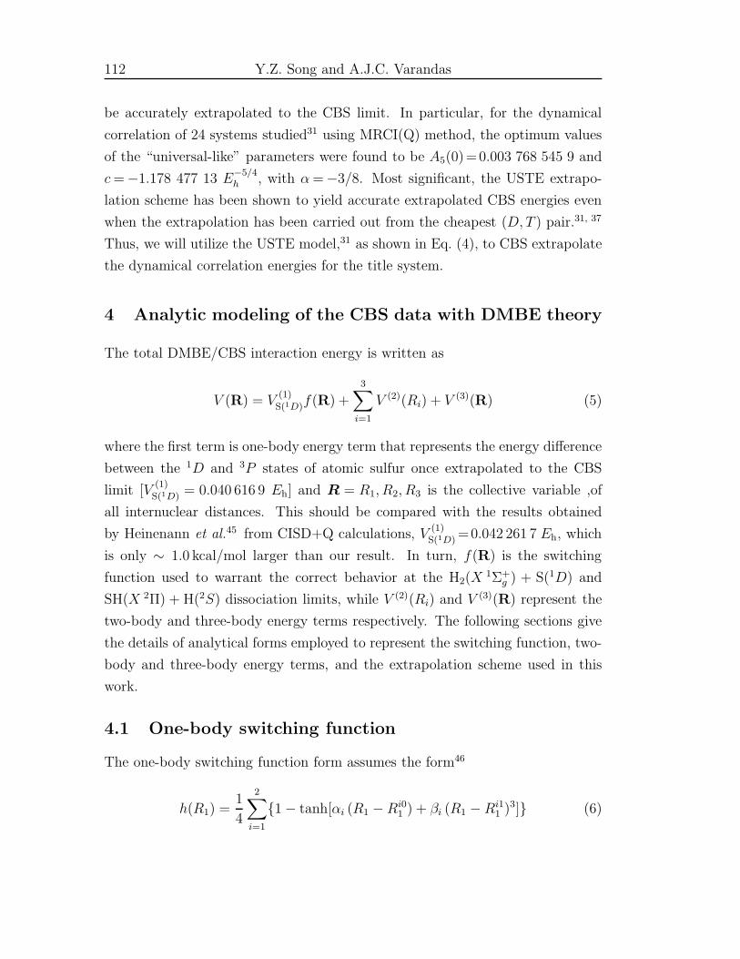
112 Y.Z. Song and A.J.C. Varandas
be accurately extrapolated to the CBS limit. In particular, for the dynamical
correlation of 24 systems studied31 using MRCI(Q) method, the optimum values
of the “universal-like” parameters were found to be A5(0) = 0.003 768 545 9 and
c= −1.178 477 13 E−5/4h , with α= −3/8. Most significant, the USTE extrapo-
lation scheme has been shown to yield accurate extrapolated CBS energies even
when the extrapolation has been carried out from the cheapest (D, T ) pair.31, 37
Thus, we will utilize the USTE model,31 as shown in Eq. (4), to CBS extrapolate
the dynamical correlation energies for the title system.
4 Analytic modeling of the CBS data with DMBE theory
The total DMBE/CBS interaction energy is written as
V (R) = V(1)
S(1D)f(R) +
3∑
i=1
V (2)(Ri) + V (3)(R) (5)
where the first term is one-body energy term that represents the energy difference
between the 1D and 3P states of atomic sulfur once extrapolated to the CBS
limit [V(1)
S(1D) = 0.040 616 9 Eh] and R = R1, R2, R3 is the collective variable ,of
all internuclear distances. This should be compared with the results obtained
by Heinenann et al.45 from CISD+Q calculations, V(1)S(1D) =0.042 261 7 Eh, which
is only ∼ 1.0 kcal/mol larger than our result. In turn, f(R) is the switching
function used to warrant the correct behavior at the H2(X1Σ+
g ) + S(1D) and
SH(X 2Π) + H(2S) dissociation limits, while V (2)(Ri) and V (3)(R) represent the
two-body and three-body energy terms respectively. The following sections give
the details of analytical forms employed to represent the switching function, two-
body and three-body energy terms, and the extrapolation scheme used in this
work.
4.1 One-body switching function
The one-body switching function form assumes the form46
h(R1) =1
4
2∑
i=1
{1 − tanh[αi (R1 − Ri01 ) + βi (R1 − Ri1
1 )3]} (6)
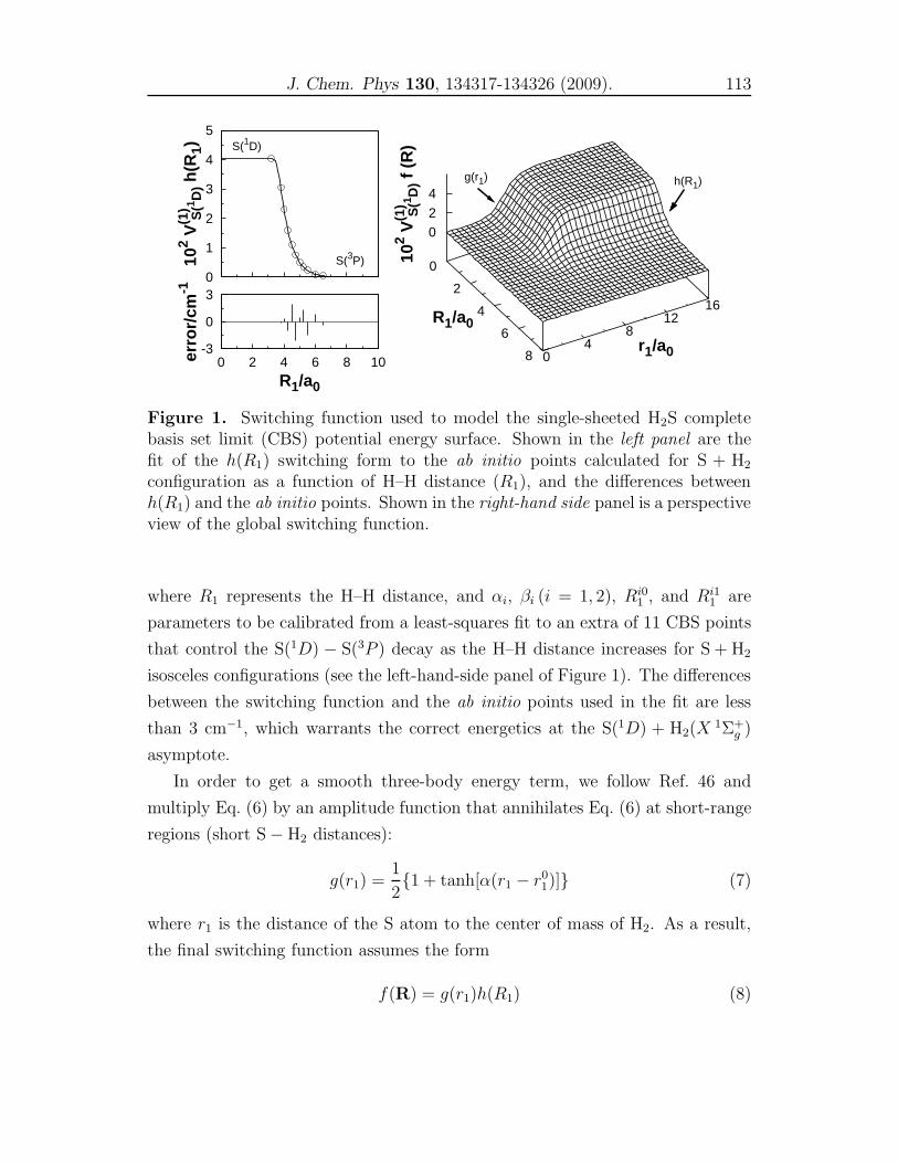
J. Chem. Phys 130, 134317-134326 (2009). 113
0
1
2
3
4
5
102 V
(1) S(1 D
) h(R
1) S(1D)
S(3P)
-3
0
3
0 2 4 6 8 10erro
r/cm
-1
R1/a0
102 V
(1) S(1 D
) f(R
)
g(r1) h(R1)
0
2
4
6
8
R1/a0
04
812
16
r1/a0
024
Figure 1. Switching function used to model the single-sheeted H2S completebasis set limit (CBS) potential energy surface. Shown in the left panel are thefit of the h(R1) switching form to the ab initio points calculated for S + H2
configuration as a function of H–H distance (R1), and the differences betweenh(R1) and the ab initio points. Shown in the right-hand side panel is a perspectiveview of the global switching function.
where R1 represents the H–H distance, and αi, βi (i = 1, 2), Ri01 , and Ri1
1 are
parameters to be calibrated from a least-squares fit to an extra of 11 CBS points
that control the S(1D) − S(3P ) decay as the H–H distance increases for S + H2
isosceles configurations (see the left-hand-side panel of Figure 1). The differences
between the switching function and the ab initio points used in the fit are less
than 3 cm−1, which warrants the correct energetics at the S(1D) + H2(X1Σ+
g )
asymptote.
In order to get a smooth three-body energy term, we follow Ref. 46 and
multiply Eq. (6) by an amplitude function that annihilates Eq. (6) at short-range
regions (short S − H2 distances):
g(r1) =1
2{1 + tanh[α(r1 − r0
1)]} (7)
where r1 is the distance of the S atom to the center of mass of H2. As a result,
the final switching function assumes the form
f(R) = g(r1)h(R1) (8)
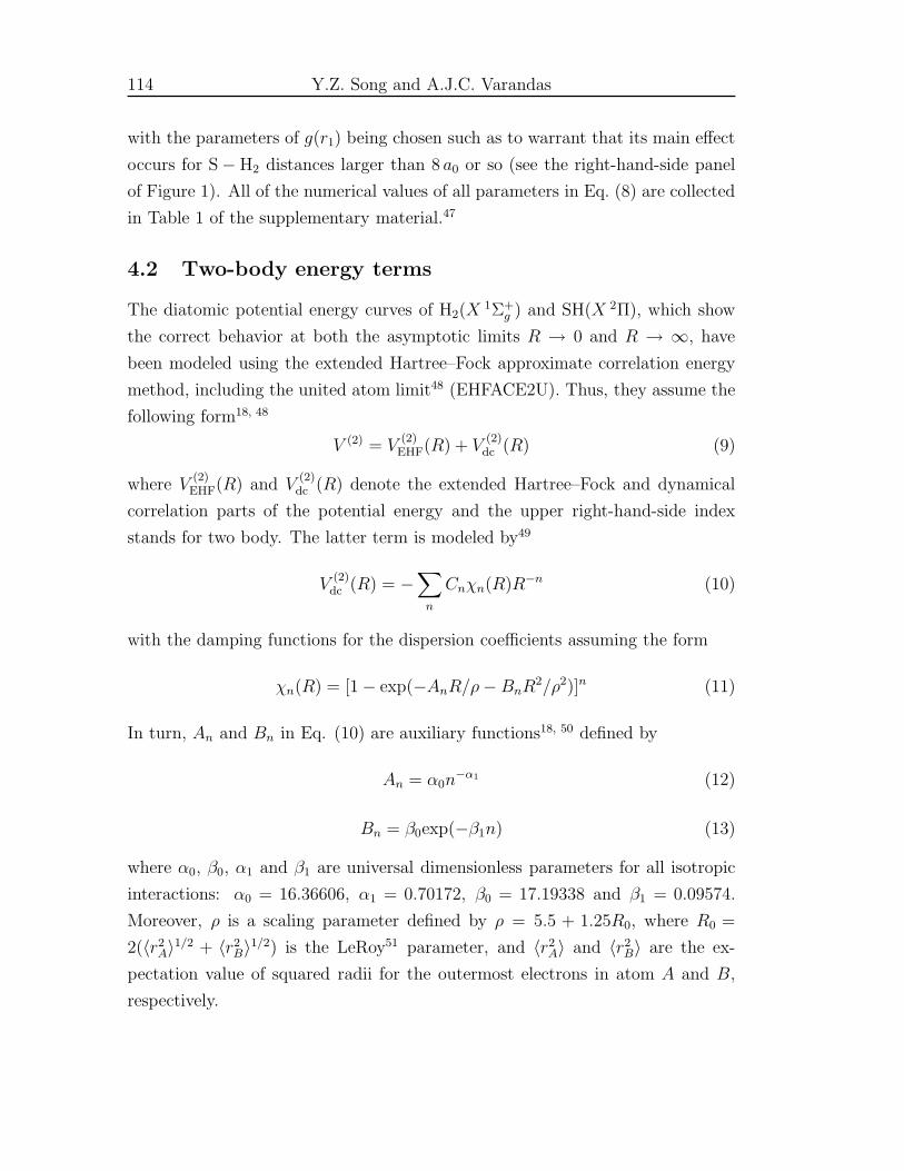
114 Y.Z. Song and A.J.C. Varandas
with the parameters of g(r1) being chosen such as to warrant that its main effect
occurs for S − H2 distances larger than 8 a0 or so (see the right-hand-side panel
of Figure 1). All of the numerical values of all parameters in Eq. (8) are collected
in Table 1 of the supplementary material.47
4.2 Two-body energy terms
The diatomic potential energy curves of H2(X 1Σ+g ) and SH(X 2Π), which show
the correct behavior at both the asymptotic limits R → 0 and R → ∞, have
been modeled using the extended Hartree–Fock approximate correlation energy
method, including the united atom limit48 (EHFACE2U). Thus, they assume the
following form18, 48
V (2) = V(2)EHF(R) + V
(2)dc (R) (9)
where V(2)EHF(R) and V
(2)dc (R) denote the extended Hartree–Fock and dynamical
correlation parts of the potential energy and the upper right-hand-side index
stands for two body. The latter term is modeled by49
V(2)dc (R) = −
∑
n
Cnχn(R)R−n (10)
with the damping functions for the dispersion coefficients assuming the form
χn(R) = [1 − exp(−AnR/ρ− BnR2/ρ2)]n (11)
In turn, An and Bn in Eq. (10) are auxiliary functions18, 50 defined by
An = α0n−α1 (12)
Bn = β0exp(−β1n) (13)
where α0, β0, α1 and β1 are universal dimensionless parameters for all isotropic
interactions: α0 = 16.36606, α1 = 0.70172, β0 = 17.19338 and β1 = 0.09574.
Moreover, ρ is a scaling parameter defined by ρ = 5.5 + 1.25R0, where R0 =
2(〈r2A〉1/2 + 〈r2
B〉1/2) is the LeRoy51 parameter, and 〈r2A〉 and 〈r2
B〉 are the ex-
pectation value of squared radii for the outermost electrons in atom A and B,
respectively.
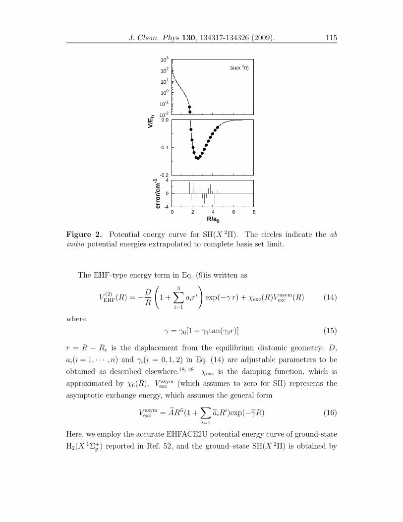
J. Chem. Phys 130, 134317-134326 (2009). 115
-0.2
-0.1
0.0
V/E
h
-4
0
4
0 2 4 6 8
err
or/
cm-1
R/a0
10-2
10-1
100
101
102
103
SH(X 2Π)
Figure 2. Potential energy curve for SH(X 2Π). The circles indicate the ab
initio potential energies extrapolated to complete basis set limit.
The EHF-type energy term in Eq. (9)is written as
V(2)EHF(R) = −D
R
(1 +
3∑
i=1
airi
)exp(−γ r) + χexc(R)V asym
exc (R) (14)
where
γ = γ0[1 + γ1tan(γ2r)] (15)
r = R − Re is the displacement from the equilibrium diatomic geometry; D,
ai(i = 1, · · · , n) and γi(i = 0, 1, 2) in Eq. (14) are adjustable parameters to be
obtained as described elsewhere.18, 48 χexc is the damping function, which is
approximated by χ6(R). V asymexc (which assumes to zero for SH) represents the
asymptotic exchange energy, which assumes the general form
V asymexc = AReα(1 +
∑
i=1
aiRi)exp(−γR) (16)
Here, we employ the accurate EHFACE2U potential energy curve of ground-state
H2(X 1Σ+g ) reported in Ref. 52, and the ground–state SH(X 2Π) is obtained by
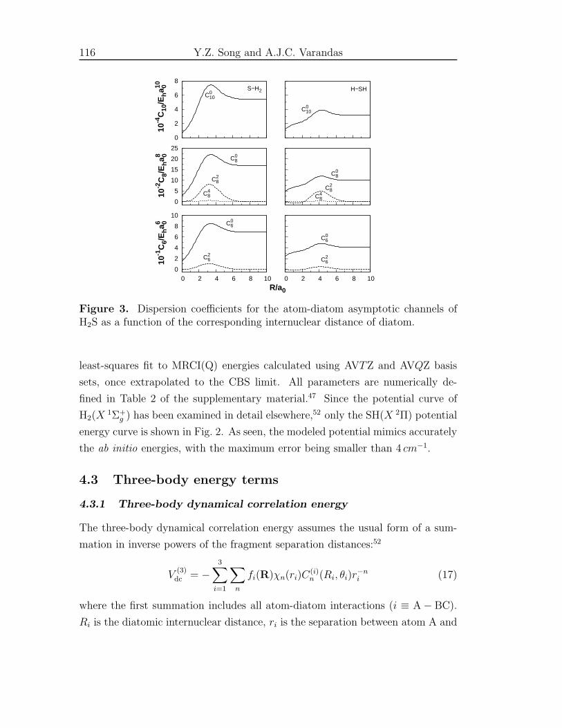
116 Y.Z. Song and A.J.C. Varandas
0
2
4
6
8
10
0 2 4 6 8 10
10-1
C6/
Eha6 0
R/a0
C26
C06
0 2 4 6 8 10
C26
C06
0
5
10
15
20
25
10-2
C8/
Eha8 0
C48
C28
C08
C48
C28
C08
0
2
4
6
8
10-4
C10
/Eha10 0
C010
S−H2
C010
H−SH
Figure 3. Dispersion coefficients for the atom-diatom asymptotic channels ofH2S as a function of the corresponding internuclear distance of diatom.
least-squares fit to MRCI(Q) energies calculated using AVTZ and AVQZ basis
sets, once extrapolated to the CBS limit. All parameters are numerically de-
fined in Table 2 of the supplementary material.47 Since the potential curve of
H2(X 1Σ+g ) has been examined in detail elsewhere,52 only the SH(X 2Π) potential
energy curve is shown in Fig. 2. As seen, the modeled potential mimics accurately
the ab initio energies, with the maximum error being smaller than 4 cm−1.
4.3 Three-body energy terms
4.3.1 Three-body dynamical correlation energy
The three-body dynamical correlation energy assumes the usual form of a sum-
mation in inverse powers of the fragment separation distances:52
V(3)dc = −
3∑
i=1
∑
n
fi(R)χn(ri)C(i)n (Ri, θi)r
−ni (17)
where the first summation includes all atom-diatom interactions (i ≡ A − BC).
Ri is the diatomic internuclear distance, ri is the separation between atom A and
J. Chem. Phys 130, 134317-134326 (2009). 117
the center-of-mass of the BC diatomic internuclear coordinate, and θi is the angle
between these two vectors (see Figure 1 of Ref. 53). fi = 12{1 − tanh[ξ(ηRi −
Rj − Rk)]} is a convenient switching function; corresponding expressions apply
to Rj , Rk, fj , and fk. Following the recent work on NH2,46 we have fixed η= 6
and ξ = 1.0 a−10 . χn(ri) is the damping function, which still takes the forms in
Eq. (11), but replace Ri by the center-of-mass separation for the relevant atom-
diatom channel, ri.
The atom-diatom dispersion coefficients in Eq. (17) is given by
C(i)n =
∑
L
CLnPL(cosθi) (18)
where PL(cosθi) denotes the L-th term of Legendre polynomial expansion and
CLn is the associated expansion coefficient. The expansion in Eq. (18) has been
truncated by considering only the coefficients C06 , C
26 , C
08 , C
28 , C
48 , and C0
10; all
other coefficients have been assumed to make a negligible contribution, and hence
neglected. To estimate the dispersion coefficients, we utilized the generalized
Slater-Kirkwood approximation54 and dipolar polarizabilities calculated in the
present work at the MRCI/AVQZ level.
As usual, the atom-diatom dispersion coefficients so calculated for a set of
nuclear distances have then been fitted to the form
CL,A−BCn (R) = CL,AB
n + CL,ACn +DM(1 +
3∑
i=1
airi)exp(−
3∑
i=1
biri) (19)
where r=R − RM is the displacement relative to the position of the maximum
and b1 = a1. CL,ABn (L = 0), the atom-atom dispersion coefficients, are given in
Table 2 of the supplementary material. Similarly, the least-squares parameters
DM , ai, and bi are collected in Table 3 of the same supplementary information.
In turn, the internuclear dependence are displayed in Fig. 3. Note that, for R=0,
the isotropic component of the dispersion coefficient is fixed at the corresponding
value in the A–X pair, where X represents the united atom of BC at the limit of
a vanishingly small internuclear separation.
As pointed out elsewhere,52 Eq. (17) causes an overestimation of the dynamical
correlation energy at the atom-diatom dissociation channel. To correct such a
behavior, we have multiplied the two-body dynamical correlation energy for i-
pair by Πj 6=i(1 − fj), correspondingly for channels j and k. This ensures that
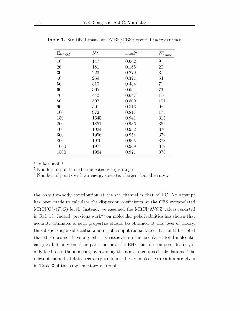
118 Y.Z. Song and A.J.C. Varandas
Table 1. Stratified rmsds of DMBE/CBS potential energy surface.
Energy Na rmsda N b>rmsd
10 147 0.062 920 181 0.185 2030 223 0.279 3740 269 0.371 5450 310 0.434 7160 365 0.631 7370 442 0.647 11080 502 0.809 10190 591 0.816 98100 972 0.817 175150 1645 0.941 315200 1861 0.936 362400 1924 0.952 370600 1956 0.954 379800 1970 0.965 3781000 1977 0.969 3791500 1984 0.971 378
a In kcal mol−1.b Number of points in the indicated energy range.c Number of points with an energy deviation larger than the rmsd.
the only two-body contribution at the ith channel is that of BC. No attempt
has been made to calculate the dispersion coefficients at the CBS extrapolated
MRCI(Q)/(T,Q) level. Instead, we assumed the MRCI/AVQZ values reported
in Ref. 13. Indeed, previous work55 on molecular polarizabilities has shown that
accurate estimates of such properties should be obtained at this level of theory,
thus dispensing a substantial amount of computational labor. It should be noted
that this does not have any effect whatsoever on the calculated total molecular
energies but only on their partition into the EHF and dc components, i.e., it
only facilitates the modeling by avoiding the above-mentioned calculations. The
relevant numerical data necessary to define the dynamical correlation are given
in Table 3 of the supplementary material.
J. Chem. Phys 130, 134317-134326 (2009). 119
4.3.2 Three-body extended Hartree-Fock energy
By removing, for a given triatomic geometry, the sum of the one-body and two-
body energy terms from the corresponding DMBE/CBS interaction energies in
Eq. (8), which was defined with respect to the infinitely separated ground-state
atoms, one obtains the total three-body energy. Then, by subtracting the three-
body dynamical correlation contribution Eq. (17) from the total three-body en-
ergy that is calculated in that way, one obtains the three-body extended Hartree-
Fock energy. This following three-body EHF energy can be represented by the
following three-body distributed-polynomial56 form
V(3)EHF =
3∑
j=1
P j(Q1, Q2, Q3) ×3∏
i=1
{1 − tanh[γji (Ri − Rj,ref
i )]} (20)
where P j(Q1, Q2, Q3) is the j-th polynomial up to six-order for j = 1, 2 and
second order for j=3. As usual, we obtain the reference geometries Rj,refi by first
assuming their values to coincide with bond distances of the associated stationary
points. Subsequently, we relax this condition via a trial-and-error least-squares
fitting procedure. Similarly, the nonlinear range-determining parameters γji have
been optimized in this way. The complete set of parameters amounts to a total
of 107 linear coefficients ci, 9 nonlinear coefficients γji , and 9 reference geometries
Rj,refi . All the numerical values of the least-squares parameters are gathered in
Table 4–6 of the supplementary material.47 Table 1 shows the stratified root-
mean-squared deviations (rmsd) values of the final potential energy surface with
respect to all the fitted ab initio energies. As shown in Table 1, a total of 1984
CBS points [as obtained from the corresponding CBS/MRCI(Q)/(T,Q) energies]
have been used for the calibration procedure, thus covering a range up to ∼1500 kcal mol−1 above the H2S global minimum. The fit shows the total root
mean square derivation is rmsd=0.97 kcal mol−1.
5 Features of the DMBE/CBS potential energy surface
Figures 4 - 8 illustrate the major topographical features of the H2S DMBE/CBS
PES reported in the present work. A characterization of their attributes (geom-
etry, energy, and vibrational frequencies) is given in Table 2 and 3. The results
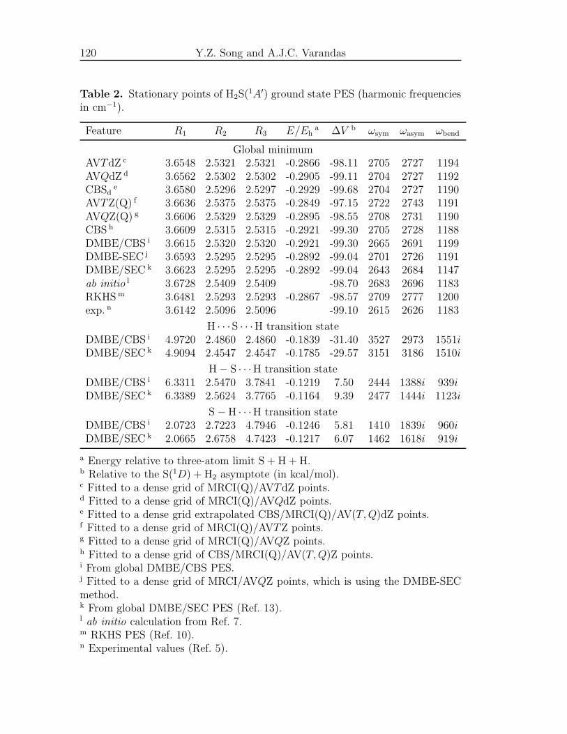
120 Y.Z. Song and A.J.C. Varandas
Table 2. Stationary points of H2S(1A′) ground state PES (harmonic frequenciesin cm−1).
Feature R1 R2 R3 E/Eha ∆V b ωsym ωasym ωbend
Global minimumAVTdZ c 3.6548 2.5321 2.5321 -0.2866 -98.11 2705 2727 1194AVQdZ d 3.6562 2.5302 2.5302 -0.2905 -99.11 2704 2727 1192CBSd
e 3.6580 2.5296 2.5297 -0.2929 -99.68 2704 2727 1190AVTZ(Q) f 3.6636 2.5375 2.5375 -0.2849 -97.15 2722 2743 1191AVQZ(Q) g 3.6606 2.5329 2.5329 -0.2895 -98.55 2708 2731 1190CBS h 3.6609 2.5315 2.5315 -0.2921 -99.30 2705 2728 1188DMBE/CBS i 3.6615 2.5320 2.5320 -0.2921 -99.30 2665 2691 1199DMBE-SEC j 3.6593 2.5295 2.5295 -0.2892 -99.04 2701 2726 1191DMBE/SEC k 3.6623 2.5295 2.5295 -0.2892 -99.04 2643 2684 1147ab initio l 3.6728 2.5409 2.5409 -98.70 2683 2696 1183RKHS m 3.6481 2.5293 2.5293 -0.2867 -98.57 2709 2777 1200exp. n 3.6142 2.5096 2.5096 -99.10 2615 2626 1183
H · · ·S · · ·H transition stateDMBE/CBS i 4.9720 2.4860 2.4860 -0.1839 -31.40 3527 2973 1551iDMBE/SEC k 4.9094 2.4547 2.4547 -0.1785 -29.57 3151 3186 1510i
H − S · · ·H transition stateDMBE/CBS i 6.3311 2.5470 3.7841 -0.1219 7.50 2444 1388i 939iDMBE/SEC k 6.3389 2.5624 3.7765 -0.1164 9.39 2477 1444i 1123i
S − H · · ·H transition stateDMBE/CBS i 2.0723 2.7223 4.7946 -0.1246 5.81 1410 1839i 960iDMBE/SEC k 2.0665 2.6758 4.7423 -0.1217 6.07 1462 1618i 919i
a Energy relative to three-atom limit S + H + H.b Relative to the S(1D) + H2 asymptote (in kcal/mol).c Fitted to a dense grid of MRCI(Q)/AVTdZ points.d Fitted to a dense grid of MRCI(Q)/AVQdZ points.e Fitted to a dense grid extrapolated CBS/MRCI(Q)/AV(T,Q)dZ points.f Fitted to a dense grid of MRCI(Q)/AVTZ points.g Fitted to a dense grid of MRCI(Q)/AVQZ points.h Fitted to a dense grid of CBS/MRCI(Q)/AV(T,Q)Z points.i From global DMBE/CBS PES.j Fitted to a dense grid of MRCI/AVQZ points, which is using the DMBE-SECmethod.k From global DMBE/SEC PES (Ref. 13).l ab initio calculation from Ref. 7.m RKHS PES (Ref. 10).n Experimental values (Ref. 5).
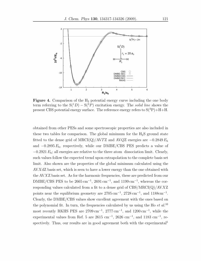
J. Chem. Phys 130, 134317-134326 (2009). 121
-14
-10
-6
-2
2
1 2 3 4 5 6
102 V
/Eh
R1/a0
S(3P) + 2H
CBSDMBE-SECDMBE/CBSDMBE/SEC
RKHS
H H
S(1D)
R1
r1 = 20a0
Figure 4. Comparison of the H2 potential energy curve including the one bodyterm referring to the S(1D) − S(3P ) excitation energy. The solid line shows thepresent CBS potential energy surface. The reference energy refers to S(3P)+H+H.
obtained from other PESs and some spectroscopic properties are also included in
these two tables for comparison. The global minimum for the H2S ground state
fitted to the dense grid of MRCI(Q)/AVTZ and AVQZ energies are −0.2849Eh
and −0.2895Eh, respectively, while our DMBE/CBS PES predicts a value of
−0.2921Eh; all energies are relative to the three atom dissociation limit. Clearly,
such values follow the expected trend upon extrapolation to the complete basis set
limit. Also shown are the properties of the global minimum calculated using the
AVXdZ basis set, which is seen to have a lower energy than the one obtained with
the AVXZ basis set. As for the harmonic frequencies, these are predicted from our
DMBE/CBS PES to be 2665 cm−1, 2691 cm−1, and 1199 cm−1, whereas the cor-
responding values calculated from a fit to a dense grid of CBS/MRCI(Q)/AVXZ
points near the equilibrium geometry are 2705 cm−1, 2728 cm−1, and 1188cm−1.
Clearly, the DMBE/CBS values show excellent agreement with the ones based on
the polynomial fit. In turn, the frequencies calculated by us using the Ho et al.10
most recently RKHS PES are 2709 cm−1, 2777 cm−1, and 1200 cm−1, while the
experimental values from Ref. 5 are 2615 cm−1, 2626 cm−1, and 1183 cm−1, re-
spectively. Thus, our results are in good agreement both with the experimental5
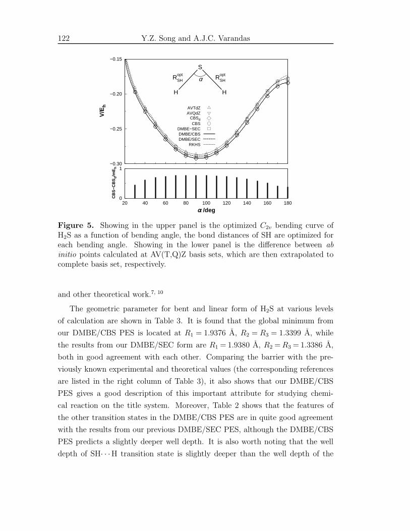
122 Y.Z. Song and A.J.C. Varandas
−0.30
−0.25
−0.20
−0.15
V/E
h AVTdZAVQdZ
CBSdCBS
DMBE−SECDMBE/CBSDMBE/SEC
RKHS
0
1
20 40 60 80 100 120 140 160 180
CB
S−C
BS
d/m
Eh
α /deg
H H
S
RoptSH Ropt
SHα
Figure 5. Showing in the upper panel is the optimized C2v bending curve ofH2S as a function of bending angle, the bond distances of SH are optimized foreach bending angle. Showing in the lower panel is the difference between ab
initio points calculated at AV(T,Q)Z basis sets, which are then extrapolated tocomplete basis set, respectively.
and other theoretical work.7, 10
The geometric parameter for bent and linear form of H2S at various levels
of calculation are shown in Table 3. It is found that the global minimum from
our DMBE/CBS PES is located at R1 = 1.9376 A, R2 = R3 = 1.3399 A, while
the results from our DMBE/SEC form are R1 = 1.9380 A, R2 =R3 = 1.3386 A,
both in good agreement with each other. Comparing the barrier with the pre-
viously known experimental and theoretical values (the corresponding references
are listed in the right column of Table 3), it also shows that our DMBE/CBS
PES gives a good description of this important attribute for studying chemi-
cal reaction on the title system. Moreover, Table 2 shows that the features of
the other transition states in the DMBE/CBS PES are in quite good agreement
with the results from our previous DMBE/SEC PES, although the DMBE/CBS
PES predicts a slightly deeper well depth. It is also worth noting that the well
depth of SH· · ·H transition state is slightly deeper than the well depth of the
J. Chem. Phys 130, 134317-134326 (2009). 123
HS· · ·H transition state, a result also in agreement with the one extracted from
our DMBE/SEC (Ref. 13) PES.
Figure 4 shows the H2 potential energy curve (including the one-body term re-
ferring to the energy difference between the 1D and 3P electronic states of atomic
sulfur). Shown by the dotted line is the H2 curve obtained by RKHS (Ref. 10)
PES, with the corresponding dissociation energy is De =−0.129 614 36Eh. This
may be compared with the value of De =−0.13136974Eh from our DMBE/SEC
PES, where the dynamical correlation energy has been corrected by scaling us-
ing the DMBE-SEC method, thus about 1.1 kcal/mol lower. In turn, the H2 +
S dissociation energy of H2 from the DMBE/CBS PES (solid line) is De =
−0.133 857 84Eh, thus 1.56 kcal/mol lower than our DMBE/SEC result. In the
long-range regions, where H2S species dissociates to three atom limit, S(3P ) +
H(2S) + H(2S), the three curves run nearly parallel to each other and show the
correct behavior. The open circles indicate the ab initio CBS/MRCI(Q) points,
clearly showing the solid line provides a high-accuracy fit to the ab initio data.
Figure 5 compares the optimized C2v bending curves for DMBE/SEC and
RKHS PES with the one obtained from the DMBE/CBS PES here reported.
Note that the latter mimics well the ab initio CBS/MRCI(Q)/(T,Q) points shown
by the open circles (these correspond to energies computed for an optimized
bond length at each value of the valence 6 HSH angle). We observe that the
DMBE/CBS PES predicts a lower well depth than the RKHS and DMBE/SEC
PESs, a trend clearly visible from Figure 5. This is not unexpected since the
Davidson correction itself for a fixed basis set has yielded slightly more attractive
energies than the DMBE-SEC method for the NH2 system.46 Table 3 gathers
the extensive work that has been done on the geometric parameters and barrier
height of linear (HSH 6 HSH = 180o). Tarczay et al.57 expected that rSH in
the linear form of H2S is shorter than the equilibrium rSH bond distance, which
is confirmed at all high levels of theory applied in their work. Nevertheless,
some of the other published PESs for H2S in Table 3 lack this feature.58–62 In
turn, the barriers for linearity calculated from these PESs58–63 are ranging from
18 792 cm−1 (Ref. 61) to 31 326 cm−1 (Ref. 62), thus showing rather big difference.
The bond distance of linear HSH from our DMBE/CBS PES is rSH = 1.3155 A,
which is also shorter than the equilibrium rSH = 1.3399 A; and the barrier to
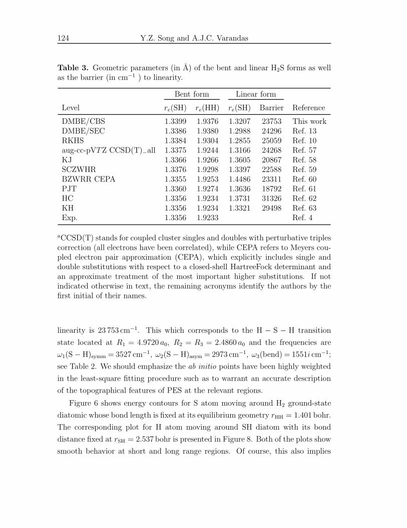
124 Y.Z. Song and A.J.C. Varandas
Table 3. Geometric parameters (in A) of the bent and linear H2S forms as wellas the barrier (in cm−1 ) to linearity.
Bent form Linear form
Level re(SH) re(HH) re(SH) Barrier Reference
DMBE/CBS 1.3399 1.9376 1.3207 23753 This workDMBE/SEC 1.3386 1.9380 1.2988 24296 Ref. 13RKHS 1.3384 1.9304 1.2855 25059 Ref. 10aug-cc-pVTZ CCSD(T)−all 1.3375 1.9244 1.3166 24268 Ref. 57KJ 1.3366 1.9266 1.3605 20867 Ref. 58SCZWHR 1.3376 1.9298 1.3397 22588 Ref. 59BZWRR CEPA 1.3355 1.9253 1.4486 23311 Ref. 60PJT 1.3360 1.9274 1.3636 18792 Ref. 61HC 1.3356 1.9234 1.3731 31326 Ref. 62KH 1.3356 1.9234 1.3321 29498 Ref. 63Exp. 1.3356 1.9233 Ref. 4
aCCSD(T) stands for coupled cluster singles and doubles with perturbative triplescorrection (all electrons have been correlated), while CEPA refers to Meyers cou-pled electron pair approximation (CEPA), which explicitly includes single anddouble substitutions with respect to a closed-shell HartreeFock determinant andan approximate treatment of the most important higher substitutions. If notindicated otherwise in text, the remaining acronyms identify the authors by thefirst initial of their names.
linearity is 23 753 cm−1. This which corresponds to the H − S − H transition
state located at R1 = 4.9720 a0, R2 = R3 = 2.4860 a0 and the frequencies are
ω1(S − H)symm = 3527 cm−1, ω2(S − H)asym = 2973 cm−1, ω3(bend) = 1551i cm−1;
see Table 2. We should emphasize the ab initio points have been highly weighted
in the least-square fitting procedure such as to warrant an accurate description
of the topographical features of PES at the relevant regions.
Figure 6 shows energy contours for S atom moving around H2 ground-state
diatomic whose bond length is fixed at its equilibrium geometry rHH = 1.401 bohr.
The corresponding plot for H atom moving around SH diatom with its bond
distance fixed at rSH = 2.537 bohr is presented in Figure 8. Both of the plots show
smooth behavior at short and long range regions. Of course, this also implies
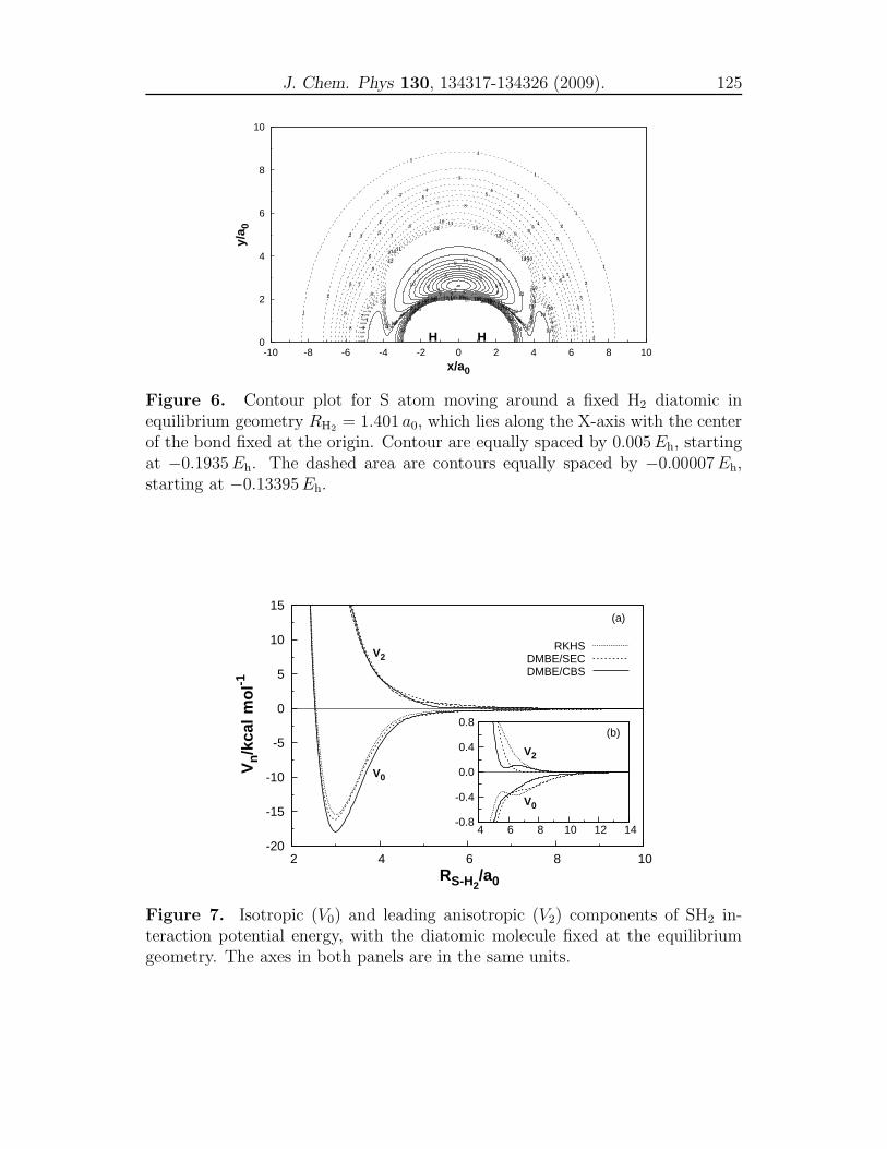
J. Chem. Phys 130, 134317-134326 (2009). 125
0
2
4
6
8
10
-10 -8 -6 -4 -2 0 2 4 6 8 10
y/a 0
x/a0
20
20
19
19
18
18
16
16
16
H
15 15
14
14
14
13
13 13
12
H
12
12
12
11
11 11
10
10
10
9
9
8
8
7
7
6
6
5
5 4 3 2
13
13
13 13 13
12
12
12
12
12
12
11
11
11
11
11
11
10
10
10
10
10
10
9
9
9 9 9
9 8
8
8
8
8
8
8
8
8
8
7
7
7
7
7
7
7
7
7
7
6
6
6
6
6
6
6
6
5
5
5
5
5
5
5 5
5
5
4 4
4
4 4
4
4
4
4 4
4
3
3
3
3
3
3
3
3
3
3
2
2
2
2
2
2
2
2
2
1
1
1 1
1
1
1
1
1
1
Figure 6. Contour plot for S atom moving around a fixed H2 diatomic inequilibrium geometry RH2
= 1.401 a0, which lies along the X-axis with the centerof the bond fixed at the origin. Contour are equally spaced by 0.005Eh, startingat −0.1935Eh. The dashed area are contours equally spaced by −0.00007Eh,starting at −0.13395Eh.
-20
-15
-10
-5
0
5
10
15
2 4 6 8 10
Vn/k
cal
mo
l-1
RS-H2/a0
V2
V0
(a)
RKHSDMBE/SECDMBE/CBS
-0.8
-0.4
0.0
0.4
0.8
4 6 8 10 12 14
V2
V0
(b)
Figure 7. Isotropic (V0) and leading anisotropic (V2) components of SH2 in-teraction potential energy, with the diatomic molecule fixed at the equilibriumgeometry. The axes in both panels are in the same units.
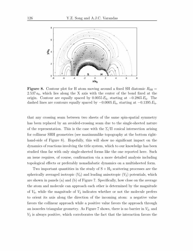
126 Y.Z. Song and A.J.C. Varandas
0
2
4
6
8
-8 -6 -4 -2 0 2 4 6 8
y/a 0
x/a0
35
34
34
33
33
32
32
31
31
S 30
30
30 29 29
29 29
28
28
H
28 27
27
27
27
27
27
26
26
26
26
26
25
25
25
25
25
24
24
24
24
24
23
23
23
23
23
22
22
22
22
22
21 21
21
21
20
20
20
20
19
19
19
19
18
18
18
18
17
17
17
16
16
16
15
15 15
14
14
14
13
13
13
12
12
11
11
11
10
10
9
9
8
8
8
7
7
6
6
5
4
4
3
2
6 6
6
6
6
6
5 5
5
5
5
5
5
4
4
4
4
4
4
4
3
3
3
3
3
3
3
3
2 2
2
2 2
2
2
2
2
2
2
1
1
1
1
1
Figure 8. Contour plot for H atom moving around a fixed SH diatomic RSH =2.537 a0, which lies along the X axis with the center of the bond fixed at theorigin. Contour are equally spaced by 0.0055Eh, starting at −0.2865Eh. Thedashed lines are contours equally spaced by −0.0005Eh, starting at −0.1395Eh.
that any crossing seam between two sheets of the same spin-spatial symmetry
has been replaced by an avoided-crossing seam due to the single-sheeted nature
of the representation. This is the case with the Σ/Π conical intersection arising
for collinear SHH geometries (see maximumlike topography at the bottom right-
hand-side of Figure 8). Hopefully, this will show no significant impact on the
dynamics of reactions involving the title system, which to our knowledge has been
studied thus far with only single-sheeted forms like the one reported here. Such
an issue requires, of course, confirmation via a more detailed analysis including
topological effects or preferably nonadiabatic dynamics on a multisheeted form.
Two important quantities in the study of S + H2 scattering processes are the
spherically averaged isotropic (V0) and leading anisotropic (V2) potentials, which
are shown in panels (a) and (b) of Figure 7. Specifically, how close on the average
the atom and molecule can approach each other is determined by the magnitude
of V0, while the magnitude of V2 indicates whether or not the molecule prefers
to orient its axis along the direction of the incoming atom: a negative value
favors the collinear approach while a positive value favors the approach through
an isosceles triangular geometry. As Figure 7 shows, there is no barrier in V2, and
V2 is always positive, which corroborates the fact that the interaction favors the
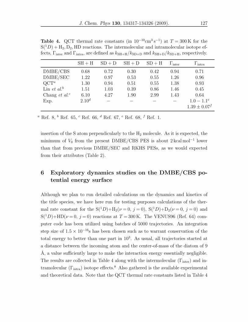
J. Chem. Phys 130, 134317-134326 (2009). 127
Table 4. QCT thermal rate constants (in 10−10cm3 s−1) at T = 300 K for theS(1D) + H2,D2,HD reactions. The intermolecular and intramolecular isotope ef-fects, Γinter and Γintra, are defined as kSH+H/kSD+D and kSH+D/kSD+H, respectively.
SH + H SD + D SH + D SD + H Γinter Γintra
DMBE/CBS 0.68 0.72 0.30 0.42 0.94 0.71DMBE/SEC 1.22 0.97 0.53 0.55 1.26 0.96QCTa 1.30 0.94 0.51 0.55 1.38 0.93Lin et al.b 1.51 1.03 0.39 0.86 1.46 0.45Chang et al.c 6.10 4.27 1.90 2.99 1.43 0.64Exp. 2.10d − − − − 1.0 − 1.1e
1.39 ± 0.07f
a Ref. 8, b Ref. 65, c Ref. 66, d Ref. 67, e Ref. 68, f Ref. 1.
insertion of the S atom perpendicularly to the H2 molecule. As it is expected, the
minimum of V0 from the present DMBE/CBS PES is about 2 kcal mol−1 lower
than that from previous DMBE/SEC and RKHS PESs, as we would expected
from their attributes (Table 2).
6 Exploratory dynamics studies on the DMBE/CBS po-
tential energy surface
Although we plan to run detailed calculations on the dynamics and kinetics of
the title species, we have here run for testing purposes calculations of the ther-
mal rate constant for the S(1D)+H2(ν = 0, j = 0), S(1D)+D2(ν = 0, j = 0) and
S(1D)+HD(ν = 0, j = 0) reactions at T = 300 K. The VENUS96 (Ref. 64) com-
puter code has been utilized using batches of 5000 trajectories. An integration
step size of 1.5 × 10⁻¹⁶s has been chosen such as to warrant conservation of the
total energy to better than one part in 103. As usual, all trajectories started at
a distance between the incoming atom and the center-of-mass of the diatom of 9
A, a value sufficiently large to make the interaction energy essentially negligible.
The results are collected in Table 4 along with the intermolecular (Γinter) and in-
tramolecular (Γintra) isotope effects.8 Also gathered is the available experimental
and theoretical data. Note that the QCT thermal rate constants listed in Table 4
128 Y.Z. Song and A.J.C. Varandas
have been divided by 5 to account for the multisurface factor, since 1D state of
S atom is five-fold degenerate.
As mentioned in the Ref. 8, 65, 66, the ordering for the isotope systems is
kH2> kHD > kD2
, a conclusion similar to the one obtained in the present work.
As can be seen, the QCT thermal rate constant for the reaction S(1D) + H2
is calculated to be 0.68 × 10⁻¹⁰cm3 s−1, which is in reasonably good agreement
with the value from our previous DMBE/SEC PES 1.22 × 10⁻¹⁰cm3 s−1 and the
experimental data 2.1 × 10⁻¹⁰cm3 s−1 by Black and Junsinski.67 In addition,
the intramolecular isotope effect Γintra = 0.71 is in excellent agreement with the
recent experiment result Γintra = 1.39 ± 0.07 from Lee et al.1 Unfortunately, no
experimental data on the intermolecular isotope effect is available that would
help confirm the good performance of our calculations in reproducing the kinetic
isotope effect for the title reaction. Yet, they match well the results from other
theoretical work.8, 65, 66
7 Concluding remarks
A global single-sheeted potential energy surface has been reported for the ground
electronic state of hydrogen sulfide on the basis of a least-squares fit to nearly
two thousand MRCI(Q) energies calculated using AVTZ and AVQZ basis sets
subsequently extrapolated to the CBS limit. The various topographical features
of the novel PES obtained via an analytical fit with DMBE theory have been
carefully examined and compared with other realistic PESs as well as experimen-
tal results available in the literature. Based on such features, it is concluded
that an accurate extrapolation to the CBS limit of the CASSCF and dynamical
correlation energies, and hence of the H2S PES, has been achieved. In summary,
the DMBE/CBS PES reported in the present work provides an accurate global
fit to all such calculated ab initio energy points. Reaction probabilities at room
temperature employing the novel DMBE/CBS PES have also been calculated for
the S(1D)+H2 and its isotopic variants S(1D)+D2 and S(1D)+HD. The results
have shown good agreement with the ones obtained from other theoretical work
and with available experimental data.
J. Chem. Phys 130, 134317-134326 (2009). 129
Acknowledgments
This work has the support of Fundacao para a Ciencia e a Tecnologia, Portu-
gal (Contract Nos. POCI/QUI/60501/ 2004 and REEQ/128/QUI/2005) under
the auspices of POCI 2010 of Quadro Comunitrio de Apoio III co-financed by
FEDER.
References
[1] S.-H. Lee and K. Liu, Chem. Phys. Let 290, 323 (1998).
[2] S.-H. Lee and K. Liu, Appl. Phys. B 71, 627 (2000).
[3] T. H. Edeards, N. K. Moncur, and L. E. Snyder, J. Chem. Phys. 46, 2139
(1967).
[4] R. L. Cook, F. C. DeLucia, and P. Helminger, J. Mol. Struct. 28, 237 (1975).
[5] M. W. Chase Jr., C. A. Davies, J. R. Downey Jr., D. J. Frurip, R. A. McDon-
ald, and A. N. Syveraud, JANAF Thermodinamic Tables, 3rd. ed. (American
Chemical Society and American Institute for Physics for the National Bureau
of Standards, New York, 1985).
[6] H. Shiina, M. Oya, K. Yamashita, A. Miyoshi, and H. Matsui, J. Phys.
Chem. 100, 2136 (1996).
[7] A. S. Zyubin, A. M. Mebel, M. Mebel, S. D. Chao, and R. T. Skodj, J. Chem.
Phys 114, 320 (2001).
[8] L. Banares, J. F. Castillo, P. Honvault, and J. Launay, Phys. Chem. Chem.
Phys. 7, 627 (2005).
[9] S. D. Chao and R. T. Skodje, J. Phys. Chem. A 105, 2474 (2001).
[10] T. S. Ho, T. Hollebeek, H. Rabitz, S. D. Chao, R. T. Skodje, A. S. Zyubin,
and A. M. Mebel, J. Chem. Phys. 116, 4124 (2002).
[11] B. Maiti, G. C. Schatz, and G. Lendvay, J. Phys. Chem. A 108, 8772 (2004).
130 Y.Z. Song and A.J.C. Varandas
[12] Y. Z. Song, A. Kinal, P. J. S. B. Caridade, A. J. C. Varandas, and P. Piecuch,
J. Mol. Struct. Theochem 859, 22 (2008).
[13] Y. Z. Song, P. J. S. B. Caridade and A. J. C. Varandas, J. Phys. Chem. A
113, 9213 (2009).
[14] H.-J. Werner and P. J. knowles, J. Chem. Phys. 89, 5803 (1988)
[15] T. H. Dunning Jr., J. Chem. Phys. 90, 1007 (1989).
[16] D. Woon and T. H. Dunning Jr., J. Chem. Phys. 98, 1358 (1993).
[17] A. J. C. Varandas, Conical Intersections: Electronic Structure, Spectroscopy
and Dynamics (World Scientific Publishing, 2004), chap. 5, p. 91, Advanced
Series in Physical Chemistry.
[18] A. J. C. Varandas, Adv. Chem. Phys. 74, 255 (1988).
[19] A. J. C. Varandas, in Lecture Notes in Chemistry , edited by A. Lagana and
A. Riganelli (Springer, Berlin, 2000), vol. 75, pp. 33–56.
[20] P. J. Knowles and H.-J. Werner, Chem. Phys. Lett. 115, 259 (1985).
[21] R. A. Kendall, T. H. Dunning Jr., and R. J. Harrison, J. Chem. Phys. 96,
6796 (1992).
[22] A. J. C. Varandas, J. Chem. Phys. 90, 4379 (1989).
[23] D. Feller, J. Chem. Phys. 96, 6104 (1992).
[24] S. S. Xantheas and T. H. Dunning Jr., J. Phys. Chem. 97, 18 (1993).
[25] D. Feller and J. A. Sordo, J. Chem. Phys. 113, 485 (2000).
[26] A. J. C. Varandas, J. Chem. Phys. 113, 8880 (2000).
[27] W. Klopper, J. Chem. Phys. 115, 761 (2001).
[28] W. Klopper, Mol. Phys. 6, 481 (2001).
[29] F. Jensen, Theoret. Chim. Acta 113, 267 (2005).
J. Chem. Phys 130, 134317-134326 (2009). 131
[30] A. Karton and J. M. L. Martin, Theoret. Chim. Acta 115, 330 (2006).
[31] A. J. C. Varandas, J. Chem. Phys. 126, 244105 (2007).
[32] A. J. C. Varandas, J. Chem. Phys. 127, 114316 (2007).
[33] A. J. C. Varandas, Chem. Phys. Lett. 443, 398 (2007).
[34] A. J. C. Varandas and P. Piecuch, Chem. Phys. Lett. 430, 448 (2006).
[35] A. J. C. Varandas, Physica Scripta 76, C28 (2007).
[36] D. W. Schwenke, J. Chem. Phys. 122, 014107 (2005).
[37] A. J. C. Varandas, J. Chem. Phys. 129, 234103 (2008).
[38] A. J. C. Varandas, Chem. Phys. Lett. 463, 225 (2008).
[39] A. J. C. Varandas, J. Comput. Chem. 30, 379 (2009).
[40] Basis sets were obtained from the Extensible Computational Chemistry Envi-
ronment Basis Set Database, Version 02/02/06, as developed and distributed
by the Molecular Science Computing Facility, Environmental and Molecu-
lar Sciences Laboratory which is part of the Pacific Northwest Laboratory,
P.O. Box 999, Richland, Washington 99352, USA, and funded by the U.S.
Department of Energy. The Pacific Northwest Laboratory is a multiprogram
laboratory operated by Battelle Memorial Institute for the U.S. Department
of Energy under contract DE-AC06-76RLO 1830. Contact Karen Schuchardt
for further information.
[41] H.-J. Werner, P. J. Knowles, R. Lindh, and et al., MOLPRO, version 2002.6,
a package of ab initio programs (2003), see http://www.molpro.net.
[42] J. M. L. Martin and O. Uzan, Chem. Phys. Lett. 282, 16 (1998).
[43] T. H. Dunning Jr., K. A. Peterson, and A. K. Wilson, J. Chem. Phys. 114,
9244 (2001).
[44] G. Tarczay, A. G. Csaszar, O. L. Polyanski, and J. Tennyson, J. Chem. Phys.
115, 1229 (2001).
132 Y.Z. Song and A.J.C. Varandas
[45] C. Heinemann, W. K loch, G.-G. Lindner, and D. Reinen, Phys. Rev. A 52,
1024 (1995).
[46] A. J. C. Varandas and L. A. Poveda, Theor. Chem. Acc. 116, 404 (2006).
[47] See EPAPS Document No. E-JCPSA6-130-034913 for the numerical data
necessary to construct the analytical DMBE/CBS potential energy sur-
face. For more information on EPAPS, see http://www.aip.org/pubservs/
epaps.html.
[48] A. J. C. Varandas and J. D. Silva, J. Chem. Soc. Faraday Trans. 88, 941
(1992).
[49] A. J. C. Varandas, Mol. Phys. 60, 527 (1987).
[50] A. J. C. Varandas, J. Mol. Struct. Theochem. 120, 401 (1985).
[51] R. J. Le Roy, Spec. Period. Rep. Chem. Soc. Mol. Spectrosc. 1, 113 (1973).
[52] A. J. C. Varandas, J. Chem. Phys. 105, 3524 (1996).
[53] A. J. C. Varandas, Chem. Phys. Lett. 194, 333 (1992).
[54] M. A. Matıas and A. J. C. Varandas, Mol. Phys. 70, 623 (1990).
[55] G. M. A. Junqueira and A. J. C. Varandas, J. Phys. Chem. A 112, 10413
(2008).
[56] E. Martınez-Nunez and A. J. C. Varandas, J. Phys. Chem. A 105, 5923
(2001).
[57] G. Tarczay, A. G. Csaszar, M. L. Leininger, and W. Klopper, Chem. Phys.
Lett 322, 119 (2000).
[58] I. Kozin and P. Jensen, J. Molec. Spectrosc. 163, 483 (1994).
[59] J. Senekowitsch, S. Carter, A. Zilch, H.-J. Werner, N. C. Handy, and P. Ros-
mus, J. Chem.Phys. 90, 783 (1989).
J. Chem. Phys 130, 134317-134326 (2009). 133
[60] P. Botschwina, A. Zilch, H.-J. Werner, P. Rosmus, and E.-A. Reinsch, J.
Chem. Phys. 85, 5107 (1986).
[61] O. L. Polyansky, P. Jensen, and J. Tennyson, J. Molec. Spectrosc. 178, 184
(1996).
[62] L. Halonen and T. Carrington Jr., J. Chem. Phys. 88, 4171 (1988).
[63] E. Kauppi and L. Halonen, J. Phys. Chem. 94, 5779 (1990).
[64] W. L. Hase, MERCURY: a general Monte-Carlo classical trajectory com-
puter program, QCPE#453. An updated version of this code is VENUS96:
W. L. Hase, R. J. Duchovic, X. Hu, A. Komornik, K. F. Lim, D.-H. Lu, G.
H. Peslherbe, K. N. Swamy, S. R. van de Linde, A. J. C. Varandas, H. Wang,
R. J. Wolf, QCPE Bull 1996, 16, 43.
[65] S. Y. Lin and H. Guo, J. Chem. Phys. 122, 074304 (2005).
[66] A. H. H. Chang and S. H. Lin, Chem. Phys. Lett. 320, 161 (2000).
[67] G. Black and L. E. Jusinski, J. Chem. Phys. 82, 789 (1985).
[68] Y. Inagaki, S. M. Shamsuddin, Y. Matsumi, and M. Kawasaki, Laser Chem.
14, 235 (1994).

J. Chem. Phys 130, 134317-134326 (2009): SI.
Accurate ab initio double many-body expansionpotential energy surface for ground-state H2S byextrapolation to the complete basis set limit
Y. Z. Song and A.J.C. Varandas
Departamento de Quımica, Universidade de Coimbra
3004-535 Coimbra Codex, Portugal.
(Received: January 15, 2009; accepted: March 2, 2009)
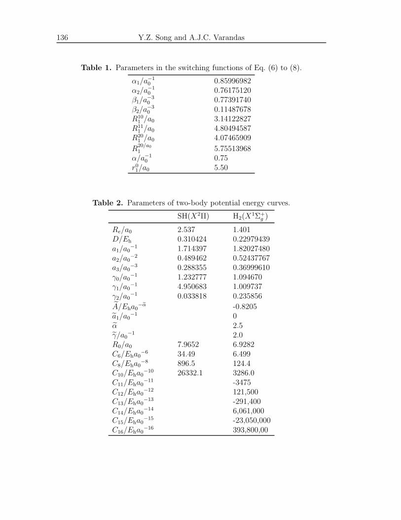
136 Y.Z. Song and A.J.C. Varandas
Table 1. Parameters in the switching functions of Eq. (6) to (8).
α1/a−10 0.85996982
α2/a−10 0.76175120
β1/a−30 0.77391740
β2/a−30 0.11487678
R101 /a0 3.14122827
R111 /a0 4.80494587
R201 /a0 4.07465909
R20/a0
1 5.75513968α/a−1
0 0.75r01/a0 5.50
Table 2. Parameters of two-body potential energy curves.
SH(X2Π) H2(X1Σ+g )
Re/a0 2.537 1.401D/Eh 0.310424 0.22979439a1/a0
−1 1.714397 1.82027480a2/a0
−2 0.489462 0.52437767a3/a0
−3 0.288355 0.36999610γ0/a0
−1 1.232777 1.094670γ1/a0
−1 4.950683 1.009737γ2/a0
−1 0.033818 0.235856
A/Eha0−eα -0.8205
a1/a0−1 0
α 2.5γ/a0
−1 2.0R0/a0 7.9652 6.9282C6/Eha0
−6 34.49 6.499C8/Eha0
−8 896.5 124.4C10/Eha0
−10 26332.1 3286.0C11/Eha0
−11 -3475C12/Eha0
−12 121,500C13/Eha0
−13 -291,400C14/Eha0
−14 6,061,000C15/Eha0
−15 -23,050,000C16/Eha0
−16 393,800,00
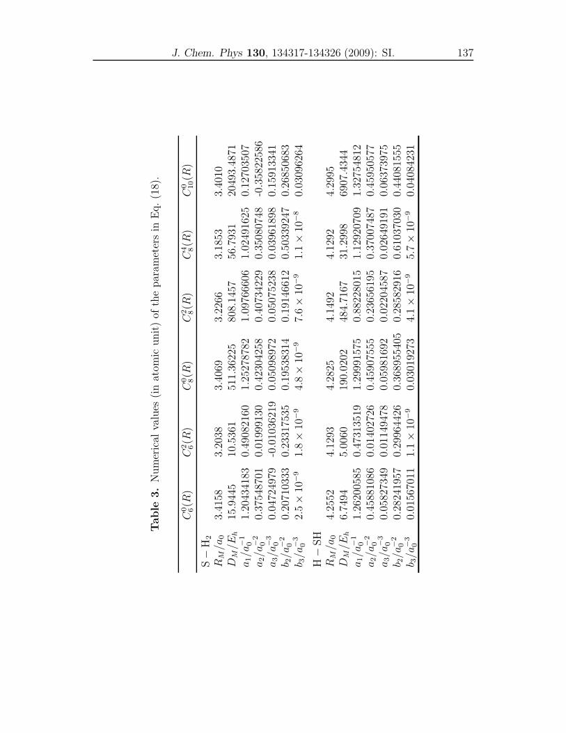
J. Chem. Phys 130, 134317-134326 (2009): SI. 137
Table
3.
Nu
mer
ical
valu
es(i
nat
omic
un
it)
ofth
ep
aram
eter
sin
Eq.
(18)
.
C0 6(R
)C
2 6(R
)C
0 8(R
)C
2 8(R
)C
4 8(R
)C
0 10(R
)
S−
H2
RM/a
03.
4158
3.20
383.
4069
3.22
663.
1853
3.40
10D
M/E
h15
.944
510
.536
151
1.36
225
808.
1457
56.7
931
2049
3.48
71a
1/a
−1
01.
2043
4183
0.49
0821
601.
2527
8782
1.09
7666
061.
0249
1625
0.12
7035
07a
2/a
−2
00.
3754
8701
0.01
9991
300.
4230
4258
0.40
7342
290.
3508
0748
-0.3
5822
586
a3/a
−3
00.
0472
4979
-0.0
1036
219
0.05
0989
720.
0507
5238
0.03
9618
980.
1591
3341
b 2/a
−2
00.
2071
0333
0.23
3175
350.
1953
8314
0.19
1466
120.
5033
9247
0.26
8506
83b 3/a
−3
02.
5×
10−
91.
8×
10−
94.
8×
10−
97.
6×
10−
91.
1×
10−
80.
0309
6264
H−
SH
RM/a
04.
2552
4.12
934.
2825
4.14
924.
1292
4.29
95D
M/E
h6.
7494
5.00
6019
0.02
0248
4.71
6731
.299
869
07.4
344
a1/a
−1
01.
2620
0585
0.47
3135
191.
2999
1575
0.88
2280
151.
1292
0709
1.32
7548
12a
2/a
−2
00.
4588
1086
0.01
4027
260.
4590
7555
0.23
6561
950.
3700
7487
0.45
9505
77a
3/a
−3
00.
0582
7349
0.01
1494
780.
0598
1692
0.02
2045
870.
0264
9191
0.06
3739
75b 2/a
−2
00.
2824
1957
0.29
9644
260.
3689
5540
50.
2858
2916
0.61
0370
300.
4408
1555
b 3/a
−3
00.
0156
7011
1.1×
10−
90.
0301
9273
4.1×
10−
95.
7×
10−
90.
0408
4231
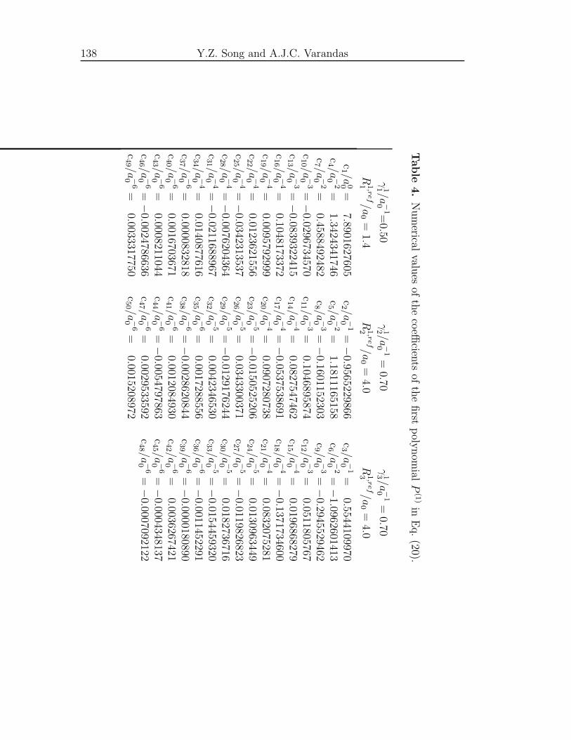
138 Y.Z. Song and A.J.C. Varandas
Table
4.
Nu
merical
values
ofth
eco
efficien
tsof
the
first
poly
nom
ialP
(1)
inE
q.
(20).
γ11 /a
−1
0=
0.50γ
12 /a−
10
=0.70
γ13 /a
−1
0=
0.70
R1,r
ef1
/a0
=1.4
R1,r
ef2
/a0
=4.0
R1,r
ef3
/a0
=4.0
c1 /a
00=
7.8901627605c2 /a
−1
0=
−0.9565229866
c3 /a
−1
0=
0.5544109970c4 /a
−2
0=
1.3424341746c5 /a
−2
0=
1.1811165158c6 /a
−2
0=
−1.0962601413
c7 /a
−2
0=
0.4588492482c8 /a
−3
0=
−0.1601152303
c9 /a
−3
0=
−0.2945529462
c10 /a
−3
0=
−0.0296734570
c11 /a
−3
0=
0.1046895874c12 /a
−3
0=
0.0511805767c13 /a
−3
0=
−0.0839322415
c14 /a
−4
0=
0.0827547462c15 /a
−4
0=
0.0196868279c16 /a
−4
0=
0.1048173372c17 /a
−4
0=
−0.0537538691
c18 /a
−4
0=
−0.1371734600
c19 /a
−4
0=
0.0095792999c20 /a
−4
0=
0.0907280738c21 /a
−4
0=
0.0832075281c22 /a
−4
0=
0.0123621556c23 /a
−5
0=
−0.0150525206
c24 /a
−5
0=
0.0130963449c25 /a
−4
0=
−0.0342313537
c26 /a
−5
0=
0.0343300371c27 /a
−5
0=
−0.0119826823
c28 /a
−4
0=
−0.0076204364
c29 /a
−5
0=
−0.0129176244
c30 /a
−5
0=
0.0182736716c31 /a
−4
0=
−0.0211688967
c32 /a
−5
0=
0.0042346530c33 /a
−5
0=
−0.0154459320
c34 /a
−4
0=
0.0140877616c35 /a
−6
0=
0.0017288556c36 /a
−6
0=
−0.0011452291
c37 /a
−6
0=
0.0000832818c38 /a
−6
0=
−0.0028620844
c39 /a
−6
0=
−0.0000180890
c40 /a
−6
0=
0.0016703671c41 /a
−6
0=
0.0012084930c42 /a
−6
0=
0.0036267421c43 /a
−6
0=
0.0008211044c44 /a
−6
0=
−0.0054797863
c45 /a
−6
0=
−0.0004348137
c46 /a
−6
0=
−0.0024786636
c47 /a
−6
0=
0.0029533592c48 /a
−6
0=
−0.0007092122
c49 /a
−6
0=
0.0033317750c50 /a
−6
0=
0.0015208972
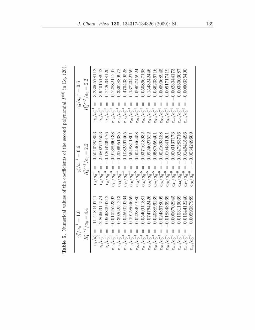
J. Chem. Phys 130, 134317-134326 (2009): SI. 139
Table
5.
Nu
mer
ical
valu
esof
the
coeffi
cien
tsof
the
seco
nd
pol
yn
omia
lP
(2)
inE
q.
(20)
.
γ2 1/a
−1
0=
1.0
γ2 2/a
−1
0=
0.6
γ2 3/a
−1
0=
0.6
R2,r
ef1
/a0
=4.
4R
2,r
ef2
/a0
=2.
2R
2,r
ef3
/a0
=2.
2
c 1/a
0 0=
−11.4
1804
9741
c 2/a
−1
0=
−0.
5040
2858
53c 3/a
−1
0=
−3.
2306
5781
12c 4/a
−2
0=
−2.
8666
3115
74c 5/a
−2
0=
−2.
6802
7195
53c 6/a
−2
0=
−3.
9401
5189
42c 7/a
−2
0=
0.96
6809
9212
c 8/a
−3
0=
−0.
1264
2091
76c 9/a
−3
0=
−0.
7426
3481
20c 1
0/a
−3
0=
−0.
0102
5223
92c 1
1/a
−3
0=
−0.
9738
9601
38c 1
2/a
−3
0=
0.72
8821
1207
c 13/a
−3
0=
−0.
3926
2512
13c 1
4/a
−4
0=
−0.
2006
9513
85c 1
5/a
−4
0=
−0.
3362
8899
72c 1
6/a
−4
0=
−0.
0459
0292
64c 1
7/a
−4
0=
0.10
8259
7465
c 18/a
−4
0=
−0.
4704
3395
28c 1
9/a
−4
0=
0.19
1586
4659
c 20/a
−4
0=
−0.
5648
8118
01c 2
1/a
−4
0=
0.13
7234
2759
c 22/a
−4
0=
−0.
0228
4919
80c 2
3/a
−5
0=
0.00
4404
6458
c 24/a
−5
0=
−0.
0962
7459
24c 2
5/a
−4
0=
−0.
0540
9118
81c 2
6/a
−5
0=
−0.
0371
6189
32c 2
7/a
−5
0=
0.05
0896
7168
c 28/a
−4
0=
−0.
0747
6424
26c 2
9/a
−5
0=
0.09
2402
7522
c 30/a
−5
0=
−0.
1543
2424
46c 3
1/a
−4
0=
0.04
0889
6239
c 32/a
−5
0=
0.06
8705
9401
c 33/a
−5
0=
0.03
6233
6716
c 34/a
−4
0=
−0.
0248
6780
09c 3
5/a
−6
0=
−0.
0021
6931
88c 3
6/a
−6
0=
−0.
0009
0689
45c 3
7/a
−6
0=
−0.
0188
4869
69c 3
8/a
−6
0=
−0.
0104
3412
01c 3
9/a
−6
0=
0.00
9171
7419
c 40/a
−6
0=
0.00
0670
2945
c 41/a
−6
0=
0.00
0313
7173
c 42/a
−6
0=
−0.
0023
0441
73c 4
3/a
−6
0=
0.01
0311
6039
c 44/a
−6
0=
−0.
0247
2837
16c 4
5/a
−6
0=
0.00
3300
3087
c 46/a
−6
0=
0.01
0441
2240
c 47/a
−6
0=
−0.
0149
4154
96c 4
8/a
−6
0=
−0.
0060
3354
90c 4
9/a
−6
0=
0.00
9908
7989
c 50/a
−6
0=
−0.
0034
2496
09
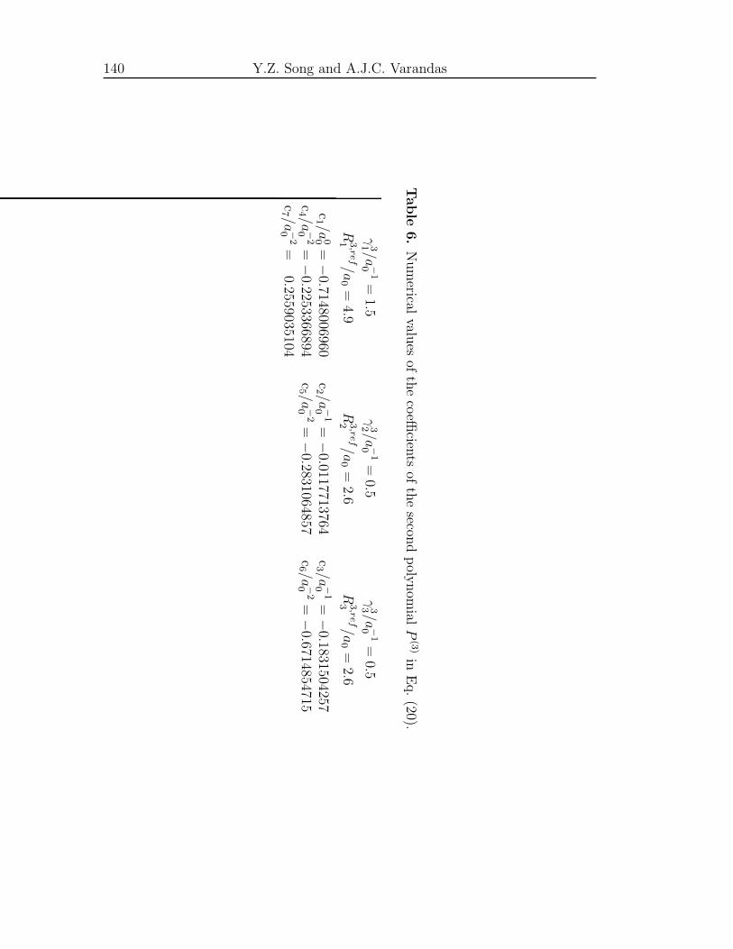
140 Y.Z. Song and A.J.C. Varandas
Table
6.
Nu
merical
values
ofth
eco
efficien
tsof
the
second
poly
nom
ialP
(3)
inE
q.
(20).
γ31 /a
−1
0=
1.5γ
32 /a−
10
=0.5
γ33 /a
−1
0=
0.5
R3,r
ef1
/a0
=4.9
R3,r
ef2
/a0
=2.6
R3,r
ef3
/a0
=2.6
c1 /a
00=
−0.7148006960
c2 /a
−1
0=
−0.0117713764
c3 /a
−1
0=
−0.1831504257
c4 /a
−2
0=
−0.2253366894
c5 /a
−2
0=
−0.2831064857
c6 /a
−2
0=
−0.6714854715
c7 /a
−2
0=
0.2559035104
Chapter 6
Accurate DMBE/SEC PES forground-state H2S

J. Phys. Chem. A 113, 9213-9219 (2009).
Potential energy surface for ground-state H2S viascaling of the external correlation, comparison withextrapolation to complete basis set limit, and use inreaction dynamics
Y. Z. Song, P. J. S. B. Caridade and A.J.C. Varandas
Departamento de Quımica, Universidade de Coimbra
3004-535 Coimbra Codex, Portugal.
(Received: April 24, 2009; Revised Manuscript Received: June 26, 2009)
Abstract
A global double many-body expansion potential energy surface is reported for the
electronic ground state of H2S by fitting accurate ab initio energies calculated at the
multireference configuration interaction level with the aug-cc-pVQZ basis set, after
slightly correcting semiempirically the dynamical correlation by the double many-body
expansion-scaled external correlation method. The function so obtained has been com-
pared in detail with a potential energy surface of the same type recently reported (Song,
Y. Z.; Varandas, A. J. C. J. Chem. Phys. 2009, 130, 134317.) by extrapolating the
calculated raw energies to the complete basis set limit, eschewing any use of information
alien to ab initio theory. The new potential energy surface is also used for studying the
dynamics and kinetics of the S(1D)+H2/D2/HD reactions.
144 Y. Z. Song, P. J. S. B. Caridade and A. J. C. Varandas
1 Introduction
The S(1D,3 P )+H2 reaction and its isotopic variants have been the subject of con-
siderable theoretical and experimental work due to its major role in environmental
issues, particularly in areas such as acid rain, air pollution, and global climate
change. Specially, the reactions of S(1D) with H2 and its isotopic are known to
proceed via an insertion path way, as demonstrated in many experimental ob-
servations1–4 and theoretical work.5–12 In a series of experiments, Inagaki et al.1
measured doppler profiles of H and D atoms from the reaction S(1D) + HD by a
laser-induced fluorescence technique with a vacuum ultraviolet laser. They have
observed an isotopic channel branching ratio of φ(SD + H)/φ(SH + D) is mea-
sured to be 0.9±0.1 for the reaction of S(1D) + HD at average collision energy of
1.2 kcal mol−1. Such a measured branching ratio and translational energy release
suggest that the reaction proceeds by insertion via formation of a long-lived com-
plex. Lee et al.2–4 measured the integral cross sections (ICSs) and vibrational
state-resolved differential cross sections (DCSs) for S(1D) + H2/D2/HD reactions
at several collision energies, which showed the ICSs decay monotonically with the
collision energy.
Theoretically, much research has been explored on the potential energy sur-
face (PES) and dynamics for the reaction S(1D) + H2.5–13 Specially, Zyubin et
al.6 obtained the electronic ground-state PES by fitting to a grid of over 2000
points based on the reproducing kernel Hilbert space (RKHS) approach and a
many-body expansion14 of the energy. The results indicate a barrierless insertion
pathway along the T-shaped geometry and an 8 kcal/mol barrier for abstrac-
tion along a collinear path. Subsequently, Chao et al.7 reported an extensive
quasiclassical trajectory (QCT) study of the S(1D) + H2/D2/HD reactions using
the PES of Zyubin et al.,6 which qualitatively reproduced the nearly symmet-
ric forward/backward DCSs, the monotonically decaying ICSs, and the product
internal state distributions observed in the experiment.2–4 Later, Ho et al.8 pro-
vided a new interpolation of the ab initio data of Zyubin et al.6 to obtain an
improved PES by fitting the same set of ab initio data, which also indicates a
barrierless insertion path along the T-shape geometry. Recently, Lin et al.12 car-
ried out quantum statistical and wave packet studies of the title reaction. The
J. Phys. Chem. A 113, 9213-9219 (2009). 145
total ICSs have been predicted to decay monotonically with the collision energy
thus supporting a barrierless insertion mechanism. Most recently,15 we reported
a PES for ground-state H2S by fitting accurate ab initio energies calculated using
Dunning’s16, 17 aug-cc-pVTZ and aug-cc-pVQZ (simply, AVTZ and AVQZ) basis
sets via extrapolation of the electron correlation energy to the complete basis set
limit (CBS) plus extrapolation to CBS of the complete-active-space self-consistent
field energy (this PES hereafter denoted as DMBE/CBS). Exploratory dynamics
calculation on the DMBE/CBS PES led to a prediction of 0.71 for the intramolec-
ular isotope effect (Γintra = kSD+H/kSH+D) for S(1D) + HD, which reproduces the
recent experiment result of Γintra = 1.39 ± 0.07 by Lee and Liu.2
In this work, we report a realistic global PES for H2S(1A′) based on DMBE18–22
theory that is calibrated from 1972 ab initio points that were calculated at the
multireference configuration interaction (MRCI)23 level, using the full valence
complete active space (FVCAS)24 reference with the AVQZ basis set. The cal-
culated ab initio energies are then corrected semiempirically using the double
many-body expansion-scaled external correlation method (DMBE-SEC)25 to ex-
trapolate to the limit of a one-electron CBS and full CI expansion and are subse-
quently modeled using DMBE theory. As usual, the resulting PES (DMBE/SEC)
shows the correct long-range behavior at all dissociation channels, while providing
an accurate fit of the calculated data at all separations.
This paper is organized as follows. Section 2 reports the ab initio calcula-
tions, and Section 3 reports the formalism used for the analytical modeling. The
discussion of its major topographical features is in Section 4, while Section 5
probes its dynamics performance when used to calculate thermal rate constants
and vibrational state-resolved ICSs. The concluding remarks are in Section 6.
2 Ab initio calculations and scaling of the external corre-
lation
The ab initio calculations have been carried out at the MRCI23 level using the
FVCAS24 wave function as reference and Dunning’s16, 17 AVQZ basis set. All cal-
culations have been performed with the Molpro26 package for electronic structure
calculation. A grid of 1972 raw ab initio points have been chosen to map the PES
146 Y. Z. Song, P. J. S. B. Caridade and A. J. C. Varandas
over the S−H2 region defined by 1.4 ≤ RH2/a0 ≤ 3.4, 1.0 ≤ rS−H2
/a0 ≤ 10.0 and
0.0 ≤ γ/ deg ≤ 90. For the H−SH interactions, a grid defined by 2.0 ≤ RSH/a0 ≤3.6, 1.0 ≤ rH−SH/a0 ≤ 10.0 and 0.0 ≤ γ/deg ≤ 180 has been chosen. As usual, r,
R and γ are the atom-diatom Jacobi coordinates for relevant channel.
The raw ab initio energies calculated above have been subsequently corrected
semiempirically with the DMBE-SEC25 method such as to account for electronic
excitations beyond singles and doubles and, most importantly, for the incom-
pleteness of the basis set. The total DMBE-SEC interaction energy assumes the
form
V (R)=VFV CAS(R) + VSEC(R) (1)
where
VFV CAS(R)=∑
AB
V(2)AB,FV CAS(RAB) + V
(3)ABC,FV CAS(RAB, RBC, RAC) (2)
VSEC(R)=∑
AB
V(2)AB,SEC(RAB) + V
(3)ABC,SEC(RAB, RBC, RAC) (3)
where R = {RAB, RBC, RAC} being a collective variable of all internuclear dis-
tances. Explicitly, the expansion of the terms in Eq. (3) assume the form:
V(2)AB,SEC(RAB)=
V(2)AB,FV CAS−CISD(RAB) − V
(2)AB,FV CAS(RAB)
F(2)AB
(4)
V(3)ABC,SEC(R)=
V(2)AB,FV CAS−CISD(R) − V
(3)ABC,FV CAS(R)
F(3)ABC
(5)
Following the previous work,25 F(2)AB in Eq. (4) is chosen to reproduce the bond
dissociation energy of the corresponding AB diatomic, while F(3)ABC in Eq. (5) is
estimated as the average of the three two-body F−factors. For the AVQZ basis
set, such a procedure yields F(2)HH =0.9773, F
(2)SH =0.8877, and F
(3)SHH =0.9176.
3 Double many-body expansion representation
Within the framework of DMBE theory,18–22 the single-sheeted PES for H2S(1A′)
assumes the form
V (R)=V(1)
S(1D)f(R) +
3∑
i=1
[V
(2)EHF(Ri) + V
(2)dc (Ri)
]+ V
(3)EHF(R) + V
(3)dc (R) (6)
J. Phys. Chem. A 113, 9213-9219 (2009). 147
where V(1)S(1D) represents the energy difference between the 1D and 3P states of
atomic sulfur: V(1)S(1D) =0.0431045Eh, f(R) is the switching function used to war-
rant the correct behavior at the H2(X 1Σ+g ) + S(1D) and SH(X 2Π) + H(2S) dis-
sociation limits. In turn, the two-body and three-body energy terms are splitted
into extended Hartree-Fock (EHF) and dynamical correlation (dc) contributions.
Because the formalism is close to the one used for the DMBE/CBS PES,15 only
a brief sketch will be presented here (see also Refs. 27, 28).
3.1 Dissociation scheme and one-body switching function
The title system has the following dissociation scheme:
H2S(1A′
) → H2 (X 1Σ+g ) + S(1D) (7)
→ SH (X 2Π) + H( 2S) (8)
Because SH (X 2Π) dissociates to ground-state atoms S(3P ) and H(2S), it is nec-
essary to introduce a function to remove the S(1D) state from this channel. Fol-
lowing Ref. 27, this is accomplished by using the switching function
f(R)=g(r1)h(R1) (9)
with the parameters of g(r1) being chosen such as to warrant that its main effect
occurs for S − H2 distances larger than 8 a0 or so (see the right-hand-side panel
of Figure 1 in the Supporting Information). In turn, the parameters in h(R1) are
calibrated from a least-squares fit to an extra of 10 AVQZ points that control
the S(1D) − S(3P ) decay with a growing H − H distance (see the left-hand-side
panel of Figure 1 in the Supporting Information). All parameters in Eq. (9) are
numerically defined in Table 1 of the Supporting Information.
3.2 Two-body energy terms
The potential energy curves of the diatomic fragments have been modeled with
the extended Hartree-Fock approximate correlation energy method including the
united atom limit (EHFACE2U),29 which shows the correct behavior at the
asymptotes R → 0 and R → ∞. Specifically, the EHF energy part assumes
148 Y. Z. Song, P. J. S. B. Caridade and A. J. C. Varandas
the form
V(2)EHF(R) = −D
R
(1 +
3∑
i=1
airi
)exp(−γ r) + χexc(R)V asym
exc (R) (10)
where
γ = γ0[1 + γ1tan(γ2r)] (11)
r = R − Re is the displacement from the equilibrium diatomic geometry; D,
ai(i = 1, · · · , n) and γi(i = 0, 1, 2) in Eq. (14) are adjustable parameters to
be obtained as described elsewhere.19, 29 χexc is the damping function, which is
approximated by χ6(R). V asymexc (which assumes to be zero for SH) represents the
asymptotic exchange energy, which assumes the general form
V asymexc = AReα(1 +
∑
i=1
aiRi)exp(−γR) (12)
In turn, the dc part is written as30
Vdc(R)=−∑
n=6,8,10
Cnχn(R)R−n (13)
where Cn are dispersion coefficients and χn are damping functions. For H2 (X 1Σ+g ),
we will utilize the accurate potential energy curve of Ref. 28, while SH (X 2Π)
is modeled from our own ab initio energies and the experimental dissociation
energy.31, 32 The relevant numerical data are gathered in Table 2 of the Support-
ing Information. Because the H2 (X 1Σ+g ) potential function is examined in detail
elsewhere,28 Figure 2 of Supporting Information illustrates only SH (X 2Π), which
is seen to mimic accurately the calculated ab initio energies.
3.3 Three-body energy terms
3.3.1 Three-body dc energy
The three-body dc energy assumes the usual form of a summation in inverse
powers of the fragment separation distances28
V(3)dc =−
∑
i
∑
n
fi(R)χn(ri)C(i)n (Ri, θi)r
−ni (14)
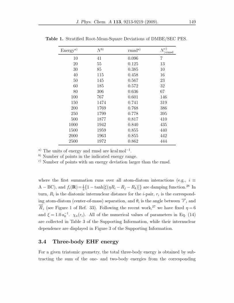
J. Phys. Chem. A 113, 9213-9219 (2009). 149
Table 1. Stratified Root-Mean-Square Deviations of DMBE/SEC PES.
Energya) N b) rmsda) Nc)>rmsd
10 41 0.096 720 55 0.125 1330 85 0.385 1040 115 0.458 1650 145 0.567 2360 185 0.572 3280 306 0.636 67
100 767 0.601 146150 1474 0.741 319200 1769 0.768 386250 1799 0.778 395500 1877 0.817 410
1000 1942 0.840 4351500 1959 0.855 4402000 1963 0.855 4422500 1972 0.862 444
a) The units of energy and rmsd are kcal mol−1.b) Number of points in the indicated energy range.c) Number of points with an energy deviation larger than the rmsd.
where the first summation runs over all atom-diatom interactions (e.g., i ≡A − BC), and fi(R)= 1
2{1− tanh[ξ(ηRi −Rj −Rk)]} are damping function.28 In
turn, Ri is the diatomic internuclear distance for the i-pair, ri is the correspond-
ing atom-diatom (center-of-mass) separation, and θi is the angle between −→r i and−→R i (see Figure 1 of Ref. 33). Following the recent work,27 we have fixed η = 6
and ξ = 1.0 a−10 . χn(ri). All of the numerical values of parameters in Eq. (14)
are collected in Table 3 of the Supporting Information, while their internuclear
dependence are displayed in Figure 3 of the Supporting Information.
3.4 Three-body EHF energy
For a given triatomic geometry, the total three-body energy is obtained by sub-
tracting the sum of the one- and two-body energies from the corresponding
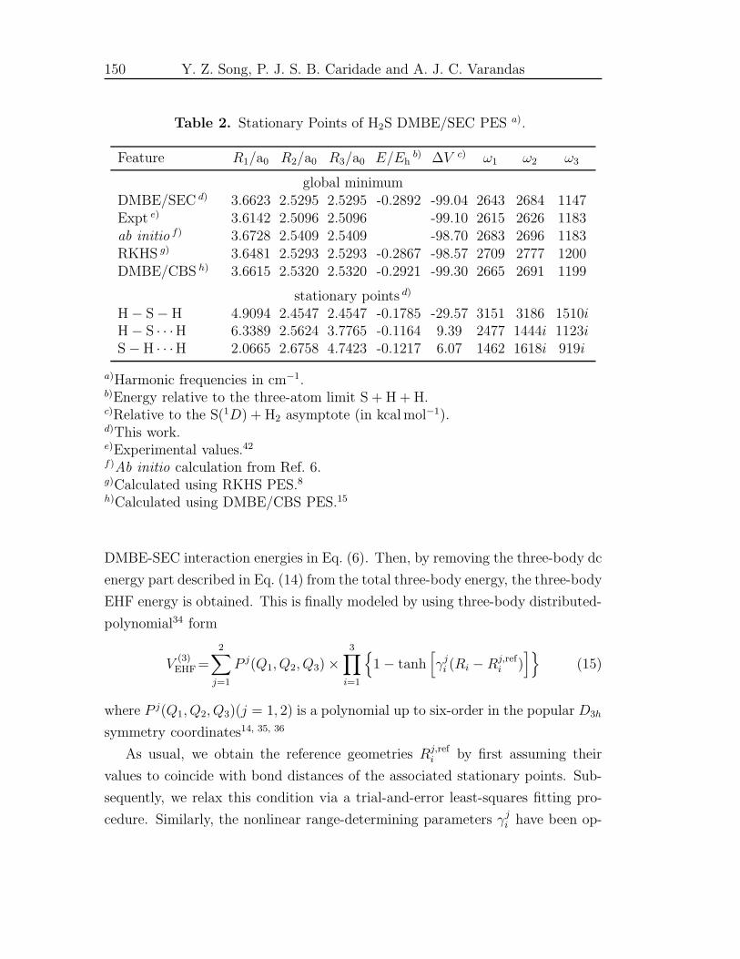
150 Y. Z. Song, P. J. S. B. Caridade and A. J. C. Varandas
Table 2. Stationary Points of H2S DMBE/SEC PES a).
Feature R1/a0 R2/a0 R3/a0 E/Ehb) ∆V c) ω1 ω2 ω3
global minimumDMBE/SEC d) 3.6623 2.5295 2.5295 -0.2892 -99.04 2643 2684 1147Expt e) 3.6142 2.5096 2.5096 -99.10 2615 2626 1183ab initio f) 3.6728 2.5409 2.5409 -98.70 2683 2696 1183RKHS g) 3.6481 2.5293 2.5293 -0.2867 -98.57 2709 2777 1200DMBE/CBS h) 3.6615 2.5320 2.5320 -0.2921 -99.30 2665 2691 1199
stationary points d)
H − S − H 4.9094 2.4547 2.4547 -0.1785 -29.57 3151 3186 1510iH − S · · ·H 6.3389 2.5624 3.7765 -0.1164 9.39 2477 1444i 1123iS − H · · ·H 2.0665 2.6758 4.7423 -0.1217 6.07 1462 1618i 919i
a)Harmonic frequencies in cm−1.b)Energy relative to the three-atom limit S + H + H.c)Relative to the S(1D) + H2 asymptote (in kcal mol−1).d)This work.e)Experimental values.42f)Ab initio calculation from Ref. 6.g)Calculated using RKHS PES.8h)Calculated using DMBE/CBS PES.15
DMBE-SEC interaction energies in Eq. (6). Then, by removing the three-body dc
energy part described in Eq. (14) from the total three-body energy, the three-body
EHF energy is obtained. This is finally modeled by using three-body distributed-
polynomial34 form
V(3)EHF =
2∑
j=1
P j(Q1, Q2, Q3) ×3∏
i=1
{1 − tanh
[γj
i (Ri − Rj,refi )
]}(15)
where P j(Q1, Q2, Q3)(j = 1, 2) is a polynomial up to six-order in the popular D3h
symmetry coordinates14, 35, 36
As usual, we obtain the reference geometries Rj,refi by first assuming their
values to coincide with bond distances of the associated stationary points. Sub-
sequently, we relax this condition via a trial-and-error least-squares fitting pro-
cedure. Similarly, the nonlinear range-determining parameters γji have been op-
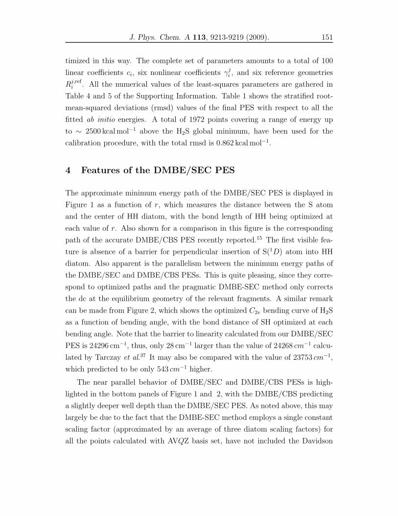
J. Phys. Chem. A 113, 9213-9219 (2009). 151
timized in this way. The complete set of parameters amounts to a total of 100
linear coefficients ci, six nonlinear coefficients γji , and six reference geometries
Rj,refi . All the numerical values of the least-squares parameters are gathered in
Table 4 and 5 of the Supporting Information. Table 1 shows the stratified root-
mean-squared deviations (rmsd) values of the final PES with respect to all the
fitted ab initio energies. A total of 1972 points covering a range of energy up
to ∼ 2500 kcal mol−1 above the H2S global minimum, have been used for the
calibration procedure, with the total rmsd is 0.862 kcal mol−1.
4 Features of the DMBE/SEC PES
The approximate minimum energy path of the DMBE/SEC PES is displayed in
Figure 1 as a function of r, which measures the distance between the S atom
and the center of HH diatom, with the bond length of HH being optimized at
each value of r. Also shown for a comparison in this figure is the corresponding
path of the accurate DMBE/CBS PES recently reported.15 The first visible fea-
ture is absence of a barrier for perpendicular insertion of S(1D) atom into HH
diatom. Also apparent is the parallelism between the minimum energy paths of
the DMBE/SEC and DMBE/CBS PESs. This is quite pleasing, since they corre-
spond to optimized paths and the pragmatic DMBE-SEC method only corrects
the dc at the equilibrium geometry of the relevant fragments. A similar remark
can be made from Figure 2, which shows the optimized C2v bending curve of H2S
as a function of bending angle, with the bond distance of SH optimized at each
bending angle. Note that the barrier to linearity calculated from our DMBE/SEC
PES is 24296 cm−1, thus, only 28 cm−1 larger than the value of 24268 cm−1 calcu-
lated by Tarczay et al.37 It may also be compared with the value of 23753 cm−1,
which predicted to be only 543 cm−1 higher.
The near parallel behavior of DMBE/SEC and DMBE/CBS PESs is high-
lighted in the bottom panels of Figure 1 and 2, with the DMBE/CBS predicting
a slightly deeper well depth than the DMBE/SEC PES. As noted above, this may
largely be due to the fact that the DMBE-SEC method employs a single constant
scaling factor (approximated by an average of three diatom scaling factors) for
all the points calculated with AVQZ basis set, have not included the Davidson
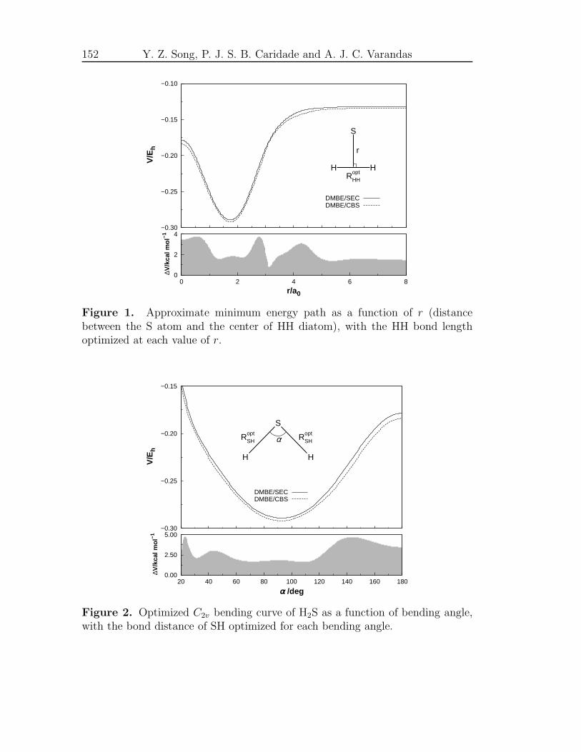
152 Y. Z. Song, P. J. S. B. Caridade and A. J. C. Varandas
−0.30
−0.25
−0.20
−0.15
−0.10
V/E
h
DMBE/SECDMBE/CBS
0
2
4
0 2 4 6 8
∆V
/kca
l mol
−1
r/a0
H H
S
RoptHH
r
Figure 1. Approximate minimum energy path as a function of r (distancebetween the S atom and the center of HH diatom), with the HH bond lengthoptimized at each value of r.
−0.30
−0.25
−0.20
−0.15
V/E
h
DMBE/SECDMBE/CBS
0.00
2.50
5.00
20 40 60 80 100 120 140 160 180
∆V
/kca
l mol
−1
α /deg
H H
S
RoptSH Ropt
SHα
Figure 2. Optimized C2v bending curve of H2S as a function of bending angle,with the bond distance of SH optimized for each bending angle.
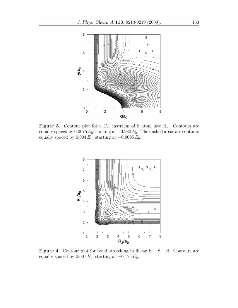
J. Phys. Chem. A 113, 9213-9219 (2009). 153
0
2
4
6
8
0 2 4 6 8
y/a 0
x/a0
42
41
41
40
40
38
38
37
37
36
35
35
34
34
33
32
32
31
30
30
29
28
28
28
27
27
26
26
26
25
25
24
24
24
23
22
22
21
21
20
19
19
18
17
17
16
15
15
14
13
12
12
11
10 9
8 7
5 4 2
H H
S
x
y
Figure 3. Contour plot for a C2v insertion of S atom into H2. Contours areequally spaced by 0.0075Eh, starting at −0.280Eh. The dashed areas are contoursequally spaced by 0.004Eh, starting at −0.0095Eh.
1
2
3
4
5
6
7
8
1 2 3 4 5 6 7 8
R3/
a 0
R2/a0
25
25 25
24
24 24
23
23
22
22
21
21
21
20
20
20 20
19
19
18
18
18 18
17
16
16
16 16
15
14
14
14 14
13
13
13 12
12
12
11
11
11 11
10
10
10 10
9
9
9
8
8
8
8
7
7 7 5
2
H S HR2 R3
Figure 4. Contour plot for bond stretching in linear H − S − H. Contours areequally spaced by 0.007Eh, starting at −0.175Eh.
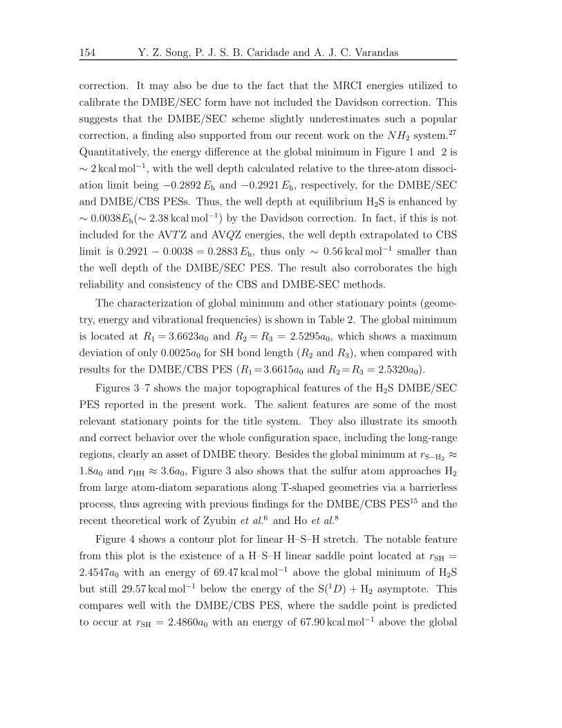
154 Y. Z. Song, P. J. S. B. Caridade and A. J. C. Varandas
correction. It may also be due to the fact that the MRCI energies utilized to
calibrate the DMBE/SEC form have not included the Davidson correction. This
suggests that the DMBE/SEC scheme slightly underestimates such a popular
correction, a finding also supported from our recent work on the NH2 system.27
Quantitatively, the energy difference at the global minimum in Figure 1 and 2 is
∼ 2 kcal mol−1, with the well depth calculated relative to the three-atom dissoci-
ation limit being −0.2892Eh and −0.2921Eh, respectively, for the DMBE/SEC
and DMBE/CBS PESs. Thus, the well depth at equilibrium H2S is enhanced by
∼ 0.0038Eh(∼ 2.38 kcal mol−1) by the Davidson correction. In fact, if this is not
included for the AVTZ and AVQZ energies, the well depth extrapolated to CBS
limit is 0.2921 − 0.0038 = 0.2883Eh, thus only ∼ 0.56 kcal mol−1 smaller than
the well depth of the DMBE/SEC PES. The result also corroborates the high
reliability and consistency of the CBS and DMBE-SEC methods.
The characterization of global minimum and other stationary points (geome-
try, energy and vibrational frequencies) is shown in Table 2. The global minimum
is located at R1 = 3.6623a0 and R2 = R3 = 2.5295a0, which shows a maximum
deviation of only 0.0025a0 for SH bond length (R2 and R3), when compared with
results for the DMBE/CBS PES (R1 =3.6615a0 and R2 =R3 = 2.5320a0).
Figures 3–7 shows the major topographical features of the H2S DMBE/SEC
PES reported in the present work. The salient features are some of the most
relevant stationary points for the title system. They also illustrate its smooth
and correct behavior over the whole configuration space, including the long-range
regions, clearly an asset of DMBE theory. Besides the global minimum at rS−H2≈
1.8a0 and rHH ≈ 3.6a0, Figure 3 also shows that the sulfur atom approaches H2
from large atom-diatom separations along T-shaped geometries via a barrierless
process, thus agreeing with previous findings for the DMBE/CBS PES15 and the
recent theoretical work of Zyubin et al.6 and Ho et al.8
Figure 4 shows a contour plot for linear H–S–H stretch. The notable feature
from this plot is the existence of a H–S–H linear saddle point located at rSH =
2.4547a0 with an energy of 69.47 kcal mol−1 above the global minimum of H2S
but still 29.57 kcal mol−1 below the energy of the S(1D) + H2 asymptote. This
compares well with the DMBE/CBS PES, where the saddle point is predicted
to occur at rSH = 2.4860a0 with an energy of 67.90 kcal mol−1 above the global
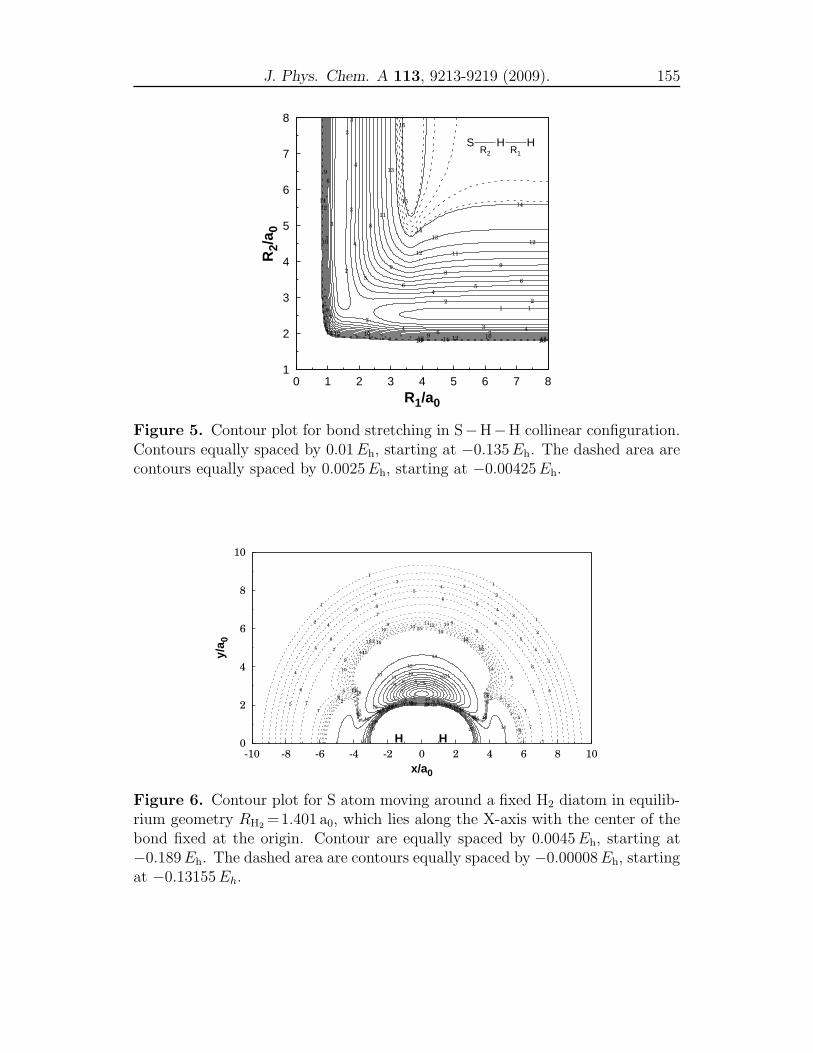
J. Phys. Chem. A 113, 9213-9219 (2009). 155
1
2
3
4
5
6
7
8
0 1 2 3 4 5 6 7 8
R2/
a 0
R1/a0
16 16
15
15
15 15
14
14 14
14
14
13
13
13 13
12
12
12
12 12
11
11
10
10 10
9 9
9
9
9
8
8
7
7 7
6 6
6
6
6
5
5
4
4
4
4 4
3
3
3
3
3
2
2
2 2
1 1
S H HR2 R1
Figure 5. Contour plot for bond stretching in S−H−H collinear configuration.Contours equally spaced by 0.01Eh, starting at −0.135Eh. The dashed area arecontours equally spaced by 0.0025Eh, starting at −0.00425Eh.
0
2
4
6
8
10
-10 -8 -6 -4 -2 0 2 4 6 8 10
y/a 0
x/a0
20
19
19
18
18
17
17
16
16
H
15
15
14
14
14
13
13
13 13
H
12
12 12
11 11
11
10 10
10
9
9
8
8
7
7
6
6
5
5
4 3 2
16
16
16
16
16
15
15
15
15
15
14
14
14
14
14
13
13
13
13
13
13
12
12
12
12
12 12
11
11
11
11
11
10
10
10
10
10
10
9 9
9
9
9
9
8
8
8
8 8
8
7
7
7
7
7
7
7
7
7
6
6
6
6
6
6
6
6
5
5 5
5
5
5
5
5
5
5
5
5
4
4
4
4
4
4
4
4
4
3
3
3
3
3
3
3
2
2 2
2
2
2
2
1 1
1
1
1
1
1
Figure 6. Contour plot for S atom moving around a fixed H2 diatom in equilib-rium geometry RH2
=1.401 a0, which lies along the X-axis with the center of thebond fixed at the origin. Contour are equally spaced by 0.0045Eh, starting at−0.189Eh. The dashed area are contours equally spaced by −0.00008Eh, startingat −0.13155Eh.
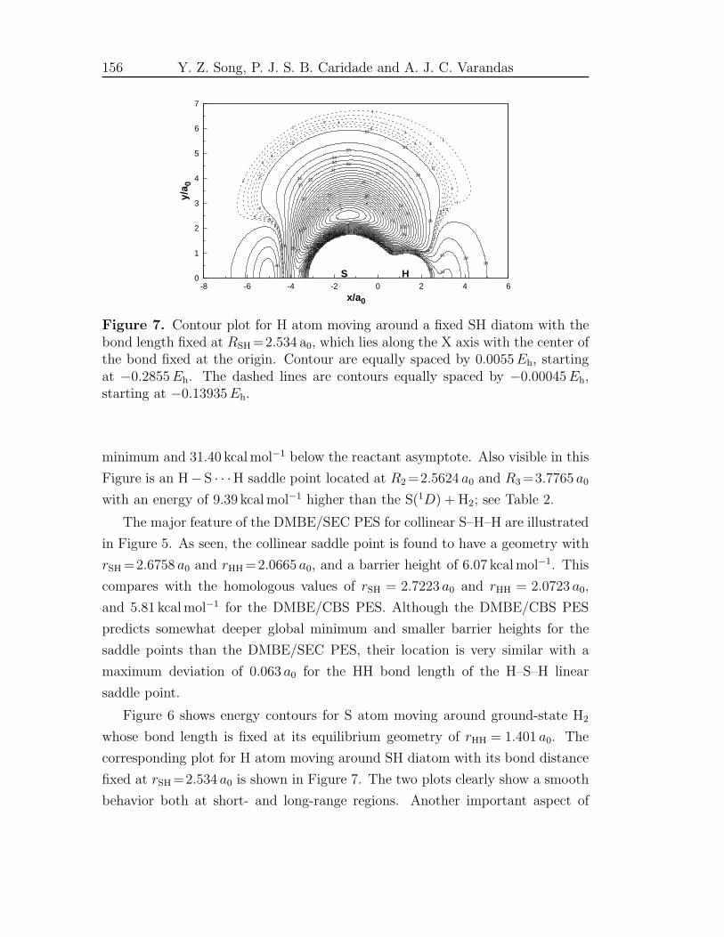
156 Y. Z. Song, P. J. S. B. Caridade and A. J. C. Varandas
0
1
2
3
4
5
6
7
-8 -6 -4 -2 0 2 4 6
y/a 0
x/a0
35
34
33
32
31
31 30
30 29
S 28
28 27
27
27
26
26
26
25
H
25
24
24
24
24
23
23
23
23
22
22
22
21
21 21
20
20
19
19
19
18
18
18 17
17
17
16
16
15
15
15
14
14 13
13
12
11
11
10 9
8
7
6
5
4
2
1
6
6
6
6
6
5 5
5
5
5 4
4
4
4
4
4
3
3
3
3
3
3
2
2
2
2
2
1
1
1
1
1
1
1
Figure 7. Contour plot for H atom moving around a fixed SH diatom with thebond length fixed at RSH =2.534 a0, which lies along the X axis with the center ofthe bond fixed at the origin. Contour are equally spaced by 0.0055Eh, startingat −0.2855Eh. The dashed lines are contours equally spaced by −0.00045Eh,starting at −0.13935Eh.
minimum and 31.40 kcal mol−1 below the reactant asymptote. Also visible in this
Figure is an H− S · · ·H saddle point located at R2 =2.5624 a0 and R3 =3.7765 a0
with an energy of 9.39 kcal mol−1 higher than the S(1D) + H2; see Table 2.
The major feature of the DMBE/SEC PES for collinear S–H–H are illustrated
in Figure 5. As seen, the collinear saddle point is found to have a geometry with
rSH =2.6758 a0 and rHH =2.0665 a0, and a barrier height of 6.07 kcal mol−1. This
compares with the homologous values of rSH = 2.7223 a0 and rHH = 2.0723 a0,
and 5.81 kcal mol−1 for the DMBE/CBS PES. Although the DMBE/CBS PES
predicts somewhat deeper global minimum and smaller barrier heights for the
saddle points than the DMBE/SEC PES, their location is very similar with a
maximum deviation of 0.063 a0 for the HH bond length of the H–S–H linear
saddle point.
Figure 6 shows energy contours for S atom moving around ground-state H2
whose bond length is fixed at its equilibrium geometry of rHH = 1.401 a0. The
corresponding plot for H atom moving around SH diatom with its bond distance
fixed at rSH =2.534 a0 is shown in Figure 7. The two plots clearly show a smooth
behavior both at short- and long-range regions. Another important aspect of
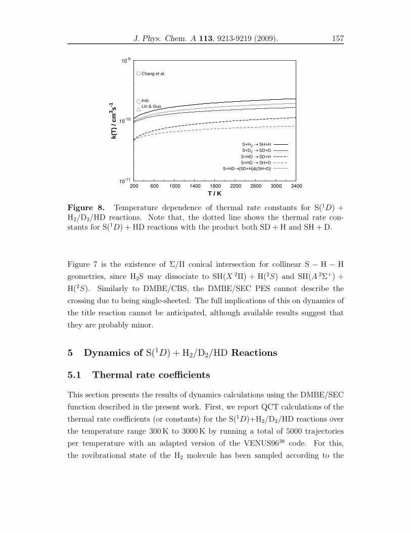
J. Phys. Chem. A 113, 9213-9219 (2009). 157
10-11
10-10
10-9
200 600 1000 1400 1800 2200 2600 3000 3400
k(T
) / c
m3 s-1
T / K
Chang et al.
exp.Lin & Guo
S+H2 ➝ SH+HS+D2 ➝ SD+D
S+HD ➝ SD+HS+HD ➝ SH+D
S+HD➝ (SD+H)&(SH+D)
Figure 8. Temperature dependence of thermal rate constants for S(1D) +H2/D2/HD reactions. Note that, the dotted line shows the thermal rate con-stants for S(1D) + HD reactions with the product both SD + H and SH + D.
Figure 7 is the existence of Σ/Π conical intersection for collinear S − H − H
geometries, since H2S may dissociate to SH(X 2Π) + H(2S) and SH(A 2Σ+) +
H(2S). Similarly to DMBE/CBS, the DMBE/SEC PES cannot describe the
crossing due to being single-sheeted. The full implications of this on dynamics of
the title reaction cannot be anticipated, although available results suggest that
they are probably minor.
5 Dynamics of S(1D) + H2/D2/HD Reactions
5.1 Thermal rate coefficients
This section presents the results of dynamics calculations using the DMBE/SEC
function described in the present work. First, we report QCT calculations of the
thermal rate coefficients (or constants) for the S(1D)+H2/D2/HD reactions over
the temperature range 300 K to 3000 K by running a total of 5000 trajectories
per temperature with an adapted version of the VENUS9638 code. For this,
the rovibrational state of the H2 molecule has been sampled according to the

158 Y. Z. Song, P. J. S. B. Caridade and A. J. C. Varandas
Table 3. Least-Squares Parameters in Eq. (16) for S+H2/D2/HD Reaction RateConstants.
A/cm3 s−1 K−n n B/K
S + H2 → SH + H 3.08 × 10⁻¹¹ 0.25 13.20S + D2 → SD + D 3.71 × 10⁻¹¹ 0.18 12.44S + HD → SH + D 1.19 × 10⁻¹¹ 0.27 13.12S + HD → SD + H 2.06 × 10⁻¹¹ 0.17 12.48
procedure of Ref. 39 but with the rovibrational partition function weighted for
the ortho-para symmetry of the hydrogen molecule. An integration step size of
1.5 × 10⁻¹⁶s has been chosen such as to warrant conservation of the total energy
to better than one part in 103. The trajectories are started at an atom-diatom
distance of 9 A, a value sufficiently large to make the interaction energy essentially
negligible.
To model the temperature dependence of the calculated rate constants, a
three-parameter Arrhenius equation has been utilized
k(T )=AT nexp(−BT
) (16)
with the parameters being numerically defined in Table 3. Figure 8 illustrates
the temperature dependence of thermal rate coefficients for the various isotopic
reactions here studied. They are found to be ordered for the various isotopes
as kH2> kHD > kD2
, at all temperatures. For S(1D)+H2 reaction at 300 K, the
rate constant is found to be 1.22 × 10⁻¹⁰cm3 s−1, thus, is in reasonably good
agreement with the experiment40 (2.1 × 10⁻¹⁰cm3 s−1) and the quantum sta-
tistical result (1.51 × 10⁻¹⁰cm3 s−1 for para-H2; 1.48 × 10⁻¹⁰cm3 s−1 for ortho-
H2) of Lin et al.12 The thermal rate constants for S(1D) + HD reaction with
the product SH + D and SD + H are calculated to be 0.53 × 10⁻¹⁰cm3 s−1 and
0.55× 10⁻¹⁰cm3 s−1, respectively. Thus, the intramolecular isotope effect defined
is Γintra = kSH+D/kSD+H = 0.96, which is slightly larger than the value of 0.71 ob-
tained from DMBE/CBS PES,15 but is close to the Lee and Liu2, 3 experimental
result of 1.39 ± 0.07 and the value of (0.9 ± 0.1) observed by Inagaki et al.1 and
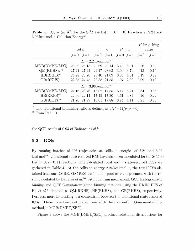
J. Phys. Chem. A 113, 9213-9219 (2009). 159
Table 4. ICS σ (in A2) for the S(1D) + H2(ν = 0, j = 0) Reaction at 2.24 and3.96 kcal mol−1 Collision Energya).
ν ′ branchingtotal ν ′ = 0 ν ′ = 1 ratio
j=0 j=1 j=0 j=1 j=0 j=1 j=0 j=1
Ec =2.24 kcal mol−1
MGB(DMBE/SEC) 26.09 26.15 20.69 20.14 5.40 6.01 0.26 0.30QM(RKHS)/b) 27.21 27.42 24.17 23.63 3.04 3.79 0.13 0.16HB(RKHS)b) 24.28 25.70 20.40 21.09 3.88 4.61 0.19 0.22GB(RKHS)b) 22.85 24.45 20.88 21.55 1.97 2.90 0.09 0.13
Ec =3.96 kcal mol−1
MGB(DMBE/SEC) 24.16 23.76 18.02 17.55 6.14 6.21 0.34 0.35HB(RKHS)b) 22.06 22.14 17.45 17.30 4.61 4.84 0.26 0.22GB(RKHS)b) 21.76 21.99 18.01 17.88 3.74 4.11 0.21 0.23
a) The vibrational branching ratio is defined as σ(ν ′=1)/σ(ν ′ =0).b) From Ref. 10.
the QCT result of 0.93 of Banares et al.11
5.2 ICSs
By running batches of 105 trajectories at collision energies of 2.24 and 3.96
kcal mol−1, vibrational state-resolved ICSs have also been calculated for the S(1D)+
H2(ν = 0, j= 0, 1) reactions. The calculated total and ν ′ state-resolved ICSs are
gathered in Table 4. At the collision energy 2.24 kcal mol−1, the total ICSs ob-
tained from our DMBE/SEC PES are found in good overall agreement with the re-
sult calculated by Banares et al.10 with quantum mechanical, QCT histogramatic
binning and QCT Gaussian-weighted binning methods using the RKHS PES of
Ho et al.8 denoted as QM(RKHS), HB(RKHS), and GB(RKHS), respectively.
Perhaps, more interesting is a comparison between the vibrational state-resolved
ICSs. These have been calculated here with the momentum Gaussian-binning
method,41 MGB(DMBE/SEC).
Figure 9 shows the MGB(DMBE/SEC) product rotational distributions for
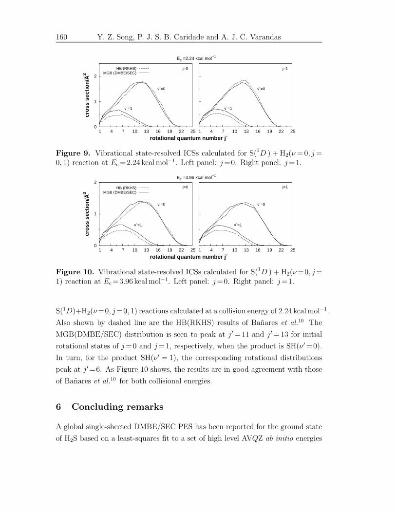
160 Y. Z. Song, P. J. S. B. Caridade and A. J. C. Varandas
0
1
2
1 4 7 10 13 16 19 22 25
cros
s se
ctio
n/Å
2
rotational quantum number j´
v´=0
v´=1
j=0
Ec =2.24 kcal mol−1
HB (RKHS)MGB (DMBE/SEC)
1 4 7 10 13 16 19 22 25
v´=0
v´=1
j=1
Figure 9. Vibrational state-resolved ICSs calculated for S(1D ) + H2(ν = 0, j=0, 1) reaction at Ec =2.24 kcal mol−1. Left panel: j=0. Right panel: j=1.
0
1
2
1 4 7 10 13 16 19 22 25
cros
s se
ctio
n/Å
2
rotational quantum number j´
v´=0
v´=1
j=0
Ec =3.96 kcal mol−1
HB (RKHS)MGB (DMBE/SEC)
1 4 7 10 13 16 19 22 25
v´=0
v´=1
j=1
Figure 10. Vibrational state-resolved ICSs calculated for S(1D ) + H2(ν=0, j=1) reaction at Ec =3.96 kcal mol−1. Left panel: j=0. Right panel: j=1.
S(1D)+H2(ν=0, j=0, 1) reactions calculated at a collision energy of 2.24 kcal mol−1.
Also shown by dashed line are the HB(RKHS) results of Banares et al.10 The
MGB(DMBE/SEC) distribution is seen to peak at j′ = 11 and j′ = 13 for initial
rotational states of j=0 and j=1, respectively, when the product is SH(ν ′ =0).
In turn, for the product SH(ν ′ = 1), the corresponding rotational distributions
peak at j′=6. As Figure 10 shows, the results are in good agreement with those
of Banares et al.10 for both collisional energies.
6 Concluding remarks
A global single-sheeted DMBE/SEC PES has been reported for the ground state
of H2S based on a least-squares fit to a set of high level AVQZ ab initio energies
J. Phys. Chem. A 113, 9213-9219 (2009). 161
that have been corrected by the DMBE-SEC method. The various topographical
features of the novel PES have been examined in detail and compared with the
DMBE/CBS PES and other PESs, as well as experimental results available in
the literature. The accuracy and consistency of the DMBE-SEC approach have
also been confirmed by comparing the corrected energies with those obtained
from CBS extrapolation to the one-electron CBS limit. Finally, the QCT ther-
mal rate constants calculated with the DMBE/SEC PES for S(1D)+H2/D2/HD
reactions have been shown to be in good agreement with available experimen-
tal and theoretical data and so did the vibrational state-resolved ICSs for the
S(1D) + H2(ν=0, j=0, 1) reactions. On the basis of the above, the DMBE/SEC
PES here reported may be recommended for dynamics studies of any type.
Having reported15 another PES for the title system out of the same raw ab
initio energies, one may wonder about their relative merits. As far as the accu-
racy of the fits is concerned, they can hardly be discriminated since they have
rather similar rmsd. Of course, the DMBE/CBS PES has been constructed in
a purely ab initio fashion, whereas the DMBE/SEC one here reported entails a
small degree of empiricism via scaling of the external (or dynamical) correlation.
The fact that they are so similar can therefore be regarded as an asset on the
consistency of both schemes. Regarding the performance of the two PESs against
experimental data, an answer must await until an extensive dynamics analysis
that goes beyond the rate constant data is reported for both. However, even then,
any superior agreement of one against the other must be qualified as discarding
nonadiabatic effects due to the single-sheeted nature of both PESs. Such studies
are currently in progress.
Acknowledgments
This work has been supported by the Fundacao para a Ciencia e Tecnologia,
Portugal.
Supporting Information Available:
Tables showing parameters and numerical values and figures showing the switch-
ing function used to model the single-sheeted H2S DMBE/SEC PES, EHFACE2U
162 Y. Z. Song, P. J. S. B. Caridade and A. J. C. Varandas
PEC for SH(X 2Π), dispersion coefficients for the atom-diatom asymptotic chan-
nels of H2S, and contour plot for bond stretching. This material is available free
of charge via the Internet at http://pubs.acs.org.
References
[1] Inagaki, Y.; Shamsuddin, S. M.; Matsumi, Y.; Kawasaki, M. Laser Chem.
1994, 14, 235–244.
[2] Lee, S.-H.; Liu, K. Chem. Phys. Let 1998, 290, 323.
[3] Lee, S.-H.; Liu, K. Appl. Phys. B 2000, 71, 627.
[4] Lee, S.-H.; Liu, K. J. Phys. Chem. A 1998, 102, 8637.
[5] Chang, A. H. H.; Lin, S. H. Chem. Phys. Lett. 2000, 320, 161.
[6] Zyubin, A. S.; Mebel, A. M.; Chao, S. D.; Skodje, R. T. J. Chem. Phys
2001, 114, 320.
[7] Chao, S. D.; Skodje, R. T. J. Phys. Chem. A 2001, 105, 2474.
[8] Ho, T.-S.; Hollebeek, T.; Rabitz, H.; Chao, S. D.; Skodje, R. T.; Zyubin,
A. S.; Mebel, A. M. J. Chem. Phys. 2002, 116, 4124.
[9] Maiti, B.; Schatz, G. C.; Lendvay, G. J. Phys. Chem. A 2004, 108, 8772.
[10] Banares, L.; Aoiz, F. J.; Honvault, P.; Launay, J.-M. J. Phys. Chem. A
2004, 108, 1616.
[11] Banares, L.; Castillo, J. F.; Honvault, P.; Launay, J.-M. Phys. Chem. Chem.
Phys. 2005, 7, 627–634.
[12] Lin, S. Y.; Guo, H. J. Chem. Phys. 2005, 122, 074304.
[13] Song, Y. Z.; Kinal, A.; Caridade, P. J. S. B.; Varandas, A. J. C.; Piecuch,
P. J. Mol. Struct. Theochem 2008, 859(1-3), 22–29.
[14] Murrell, J. N.; Carter, S.; Farantos, S. C.; Huxley, P.; Varandas, A. J. C.
Molecular Potential Energy Functions; Wiley: Chichester, 1984.
J. Phys. Chem. A 113, 9213-9219 (2009). 163
[15] Song, Y. Z.; Varandas, A. J. C. J. Chem. Phys. 2009, 130, 134317.
[16] Kendall, R. A.; Dunning Jr., T. H.; Harrison, R. J. J. Chem. Phys. 1992,
96, 6769.
[17] Dunning Jr., T. H. J. Chem. Phys. 1989, 90, 1007.
[18] Varandas, A. J. C.; World Scientific Publishing, 2004; chapter 5, p 91;
Advanced Series in Physical Chemistry.
[19] Varandas, A. J. C. Adv. Chem. Phys. 1988, 74, 255.
[20] Varandas, A. J. C. J. Mol. Struct. Theochem. 19850, 120, 401.
[21] Varandas, A. J. C. Mol. Phys. 1984, 53, 1303.
[22] Varandas, A. J. C. Lecture Notes in Chemistry; Lagana, A., Riganelli, A.,
Eds.; Springer: Berlin, 2000; Vol. 75, pp 33–56.
[23] Werner, H.-J.; Knowles, P. J. J. Chem. Phys. 1988, 89, 5803.
[24] Knowles, P. J.; Werner, H.-J. Chem. Phys. Lett. 1985, 115, 259.
[25] Varandas, A. J. C. J. Chem. Phys. 1989, 90, 4379–4391.
[26] Werner, H.-J.; Knowles, P. J.; Lindh, R.; Schutz, M.; Celani, P.; Korona,
T.; Manby, F. R.; Rauhut, G.; Amos, R. D.; Bernhardsson, A.; Berning,
A.; Cooper, D. L.; Deegan, M. J. O.; Dobbyn, A. J.; Eckert, F.; Hampel,
C.; Hetzer, G.; Lloyd, A. W.; McNicholas, S. J.; Meyer, W.; Mura, M. E.;
Nicklass, A.; Palmieri, P.; Pitzer, R.; Schumann, U.; Stoll, H.; Stone, A. J.;
Tarroni, R.; Thorsteinsson, T., Molpro, version 2002.6, a package of ab initio
programs. 2003.
[27] Varandas, A. J. C.; Poveda, L. A. Theor. Chem. Acc. 2006, 116, 404.
[28] Varandas, A. J. C. J. Chem. Phys. 1996, 105, 3524.
[29] Varandas, A. J. C.; Silva, J. D. J. Chem. Soc. Faraday Trans. 1992, 88, 941.
[30] Varandas, A. J. C. Mol. Phys. 1987, 60, 527.
164 Y. Z. Song, P. J. S. B. Caridade and A. J. C. Varandas
[31] Huber, K. P.; Herzberg, G., Molecular spectra and molecular structure con-
stants of diatomic molecules (van nostrand reinhold, New York, 1979).
[32] Lodders, K. J. Phys. Chem. Ref. Data. 2004, 33, 357.
[33] Varandas, A. J. C. Chem. Phys. Lett. 1992, 194, 333.
[34] Martınez-Nunez, E.; Varandas, A. J. C. J. Phys. Chem. A 2001, 105, 5923–
5932.
[35] Murrell, J. N.; Sorbie, K. S.; Varandas, A. J. C. Mol. Phys. 1976, 32, 1359.
[36] Varandas, A. J. C.; Murrell, J. N. Faraday Discuss. Chem. Soc. 1977, 62,
92.
[37] Tarczay, G.; Csaszar, A. G.; Leininger, M. L.; Klopper, W. Chem. Phys.
Lett. 2000, 322, 119.
[38] Hase, W. L.; Duchovic, R. J.; Hu, X.; Komornicki, A.; Lim, K. F.; Lu, D.;
Peslherbe, G. H.; Swamy, K. N.; Linde, S. R. V.; Varandas, A. J. C.; Wang,
H.; Wolf, R. J. QCPE Bull. 1996, 16, 43.
[39] Caridade, P. J. S. B.; Varandas, A. J. C. J. Phys. Chem. A 2004, 108, 3556.
[40] Black, G.; Jusinski, L. E. J. Chem. Phys. 1985, 82, 789.
[41] Varandas, A. J. C. Chem. Phys. Lett. 2007, 439, 386.
[42] Chase Jr., M. W.; Davies, C. A.; Downey Jr., J. R.; Frurip, D. J.; McDonald,
R. A.; Syveraud, A. N. JANAF Thermodinamic Tables, 3rd. ed.; American
Chemical Society and American Institute for Physics for the National Bureau
of Standards: New York, 1985.
J. Phys. Chem. A 113, 9213-9219 (2009): SI.
Potential energy surface for ground-state H2S viascaling of the external correlation, comparison withextrapolation to complete basis set limit, and use inreaction dynamics
Y. Z. Song, P. J. S. B. Caridade and A.J.C. Varandas
Departamento de Quımica, Universidade de Coimbra
3004-535 Coimbra Codex, Portugal.
(Received: April 24, 2009; Revised Manuscript Received: June 26, 2009)
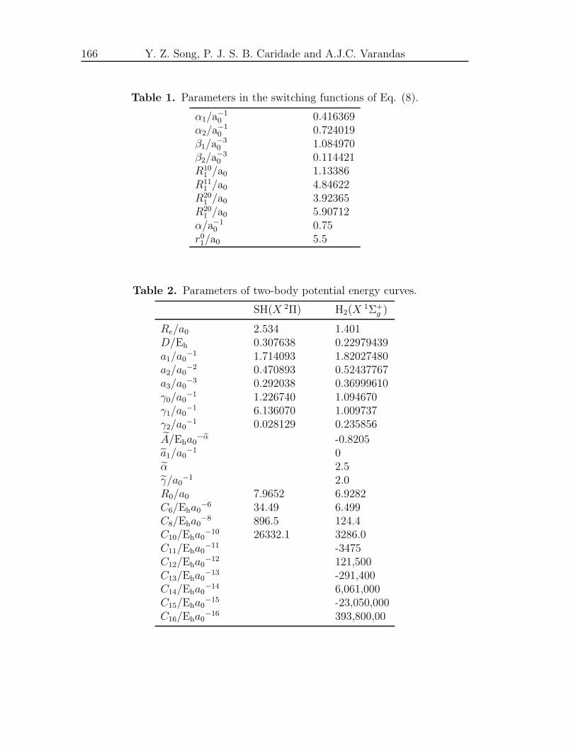
166 Y. Z. Song, P. J. S. B. Caridade and A.J.C. Varandas
Table 1. Parameters in the switching functions of Eq. (8).
α1/a−10 0.416369
α2/a−10 0.724019
β1/a−30 1.084970
β2/a−30 0.114421
R101 /a0 1.13386
R111 /a0 4.84622
R201 /a0 3.92365
R201 /a0 5.90712
α/a−10 0.75
r01/a0 5.5
Table 2. Parameters of two-body potential energy curves.
SH(X 2Π) H2(X 1Σ+g )
Re/a0 2.534 1.401D/Eh 0.307638 0.22979439a1/a0
−1 1.714093 1.82027480a2/a0
−2 0.470893 0.52437767a3/a0
−3 0.292038 0.36999610γ0/a0
−1 1.226740 1.094670γ1/a0
−1 6.136070 1.009737γ2/a0
−1 0.028129 0.235856
A/Eha0−eα -0.8205
a1/a0−1 0
α 2.5γ/a0
−1 2.0R0/a0 7.9652 6.9282C6/Eha0
−6 34.49 6.499C8/Eha0
−8 896.5 124.4C10/Eha0
−10 26332.1 3286.0C11/Eha0
−11 -3475C12/Eha0
−12 121,500C13/Eha0
−13 -291,400C14/Eha0
−14 6,061,000C15/Eha0
−15 -23,050,000C16/Eha0
−16 393,800,00

J. Phys. Chem. A 113, 9213-9219 (2009): SI. 167
Table
3.
Nu
mer
ical
valu
es(i
nat
omic
un
it)
ofth
ep
aram
eter
sin
Eq.
(18)
.
C0 6(R
)C
2 6(R
)C
0 8(R
)C
2 8(R
)C
4 8(R
)C
0 10(R
)
S−
H2
RM/a
03.
4158
3.20
383.
4069
3.22
663.
1853
3.40
10D
M/E
h15
.944
510
.536
151
1.36
225
808.
1457
56.7
931
2049
3.48
71a
1/a
−1
01.
2043
4183
0.49
0821
601.
2527
8782
1.09
7666
061.
0249
1625
0.12
7035
07a
2/a
−2
00.
3754
8701
0.01
9991
300.
4230
4258
0.40
7342
290.
3508
0748
-0.3
5822
586
a3/a
−3
00.
0472
4979
-0.0
1036
219
0.05
0989
720.
0507
5238
0.03
9618
980.
1591
3341
b 2/a
−2
00.
2071
0333
0.23
3175
350.
1953
8314
0.19
1466
120.
5033
9247
0.26
8506
83b 3/a
−3
02.
5×
10−
91.
8×
10−
94.
8×
10−
97.
6×
10−
91.
1×
10−
80.
0309
6264
H−
SH
RM/a
04.
2552
4.12
934.
2825
4.14
924.
1292
4.29
95D
M/E
h6.
7494
5.00
6019
0.02
0248
4.71
6731
.299
869
07.4
344
a1/a
−1
01.
2620
0585
0.47
3135
191.
2999
1575
0.88
2280
151.
1292
0709
1.32
7548
12a
2/a
−2
00.
4588
1086
0.01
4027
260.
4590
7555
0.23
6561
950.
3700
7487
0.45
9505
77a
3/a
−3
00.
0582
7349
0.01
1494
780.
0598
1692
0.02
2045
870.
0264
9191
0.06
3739
75b 2/a
−2
00.
2824
1957
0.29
9644
260.
3689
5540
50.
2858
2916
0.61
0370
300.
4408
1555
b 3/a
−3
00.
0156
7011
1.1×
10−
90.
0301
9273
4.1×
10−
95.
7×
10−
90.
0408
4231
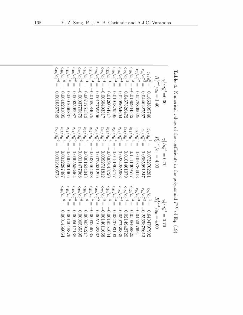
168 Y. Z. Song, P. J. S. B. Caridade and A.J.C. Varandas
Table
4.
Nu
merical
values
ofth
eco
efficien
tsin
the
poly
nom
ialP
(1)
ofE
q.
(19).
γ11 /a
−1
0=
0.30γ
12 /a−
10
=0.70
γ13 /a
−1
0=
0.70
R1,ref
1/a
0=
1.40R
1,ref
2/a
0=
4.00R
1,ref
3/a
0=
4.00
c1 /a
00=
0.1863809740c2 /a
−1
0=
0.0732702281c3 /a
−1
0=
0.6404797902c4 /a
−2
0=
0.0446227567c5 /a
−2
0=
0.0685991247c6 /a
−2
0=−
0.2569878613c7 /a
−2
0=
0.0578809025c8 /a
−3
0=
0.0059786913c9 /a
−3
0=−
0.0450976941c10 /a
−3
0=−
0.0180934342c11 /a
−3
0=
0.1111309577c12 /a
−3
0=
0.0508468820c13 /a
−3
0=
0.0457526472c14 /a
−4
0=
0.0101461079c15 /a
−4
0=
0.0214942720c16 /a
−4
0=
0.0209654604c17 /a
−4
0=
0.0234285683c18 /a
−4
0=−
0.0507736835c19 /a
−4
0=
0.0191879595c20 /a
−4
0=−
0.0151803777c21 /a
−4
0=
0.0343793193c22 /a
−4
0=
0.0126054717c23 /a
−5
0=−
0.0009143720c24 /a
−5
0=−
0.0019551634c25 /a
−4
0=−
0.0060493317c26 /a
−5
0=
0.0092731812c27 /a
−5
0=−
0.0014011668c28 /a
−4
0=
0.0017759506c29 /a
−5
0=−
0.0073031290c30 /a
−5
0=
0.0051938362c31 /a
−4
0=−
0.0168584075c32 /a
−5
0=−
0.0037464038c33 /a
−5
0=−
0.0003256735c34 /a
−4
0=
0.0071751313c35 /a
−6
0=
0.0001634043c36 /a
−6
0=
0.0009391217c37 /a
−6
0=−
0.0003775879c38 /a
−6
0=−
0.0011477968c39 /a
−6
0=
0.0006535595c40 /a
−6
0=
0.0003599987c41 /a
−6
0=
0.0005556464c42 /a
−6
0=−
0.0005017138c43 /a
−6
0=
0.0001666837c44 /a
−6
0=−
0.0006301966c45 /a
−6
0=
0.0010048876c46 /a
−6
0=
0.0010231005c47 /a
−6
0=
0.0012287487c48 /a
−6
0=
0.0001456064c49 /a
−6
0=
0.0010567549c50 /a
−6
0=
0.0012160573
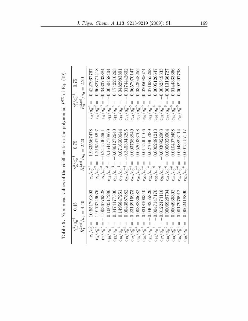
J. Phys. Chem. A 113, 9213-9219 (2009): SI. 169
Table
5.
Nu
mer
ical
valu
esof
the
coeffi
cien
tsin
the
pol
yn
omia
lP
(2)
ofE
q.
(19)
.
γ2 1/a
−1
0=
0.45
γ2 2/a
−1
0=
0.75
γ2 3/a
−1
0=
0.75
R2,r
ef1
/a0
=4.
40R
2,r
ef2
/a0
=2.
20R
2,r
ef3
/a0
=2.
20
c 1/a
0 0=−
10.5
5179
1893
c 2/a
−1
0=−
1.93
3556
7478
c 3/a
−1
0=−
0.42
2796
7767
c 4/a
−2
0=−
1.91
7374
9076
c 5/a
−2
0=−
1.21
9547
9297
c 6/a
−2
0=
0.96
8277
1418
c 7/a
−2
0=−
1.00
3677
6328
c 8/a
−3
0=−
0.24
1506
2961
c 9/a
−3
0=−
0.34
3373
3884
c 10/a
−3
0=
0.10
0351
7286
c 11/a
−3
0=
0.16
4477
0879
c 12/a
−3
0=−
0.00
5045
8404
c 13/a
−3
0=
0.34
7417
7500
c 14/a
−4
0=−
0.08
6127
2640
c 15/a
−4
0=
0.17
4221
0263
c 16/a
−4
0=
0.14
9584
7251
c 17/a
−4
0=
0.07
1660
0644
c 18/a
−4
0=
0.04
8298
3891
c 19/a
−4
0=
0.00
4358
7882
c 20/a
−4
0=−
0.34
5394
3295
c 21/a
−4
0=−
0.01
7444
2602
c 22/a
−4
0=−
0.23
1391
5973
c 23/a
−5
0=
0.00
3758
3849
c 24/a
−5
0=
0.06
5797
0147
c 25/a
−4
0=−
0.00
3883
0682
c 26/a
−5
0=
0.05
2003
3708
c 27/a
−5
0=
0.03
4394
8252
c 28/a
−4
0=−
0.03
1810
0340
c 29/a
−5
0=
0.01
1500
1166
c 30/a
−5
0=−
0.02
0508
5674
c 31/a
−4
0=−
0.04
6825
5826
c 32/a
−5
0=
0.02
7096
5389
c 33/a
−5
0=
0.07
1985
5268
c 34/a
−4
0=−
0.00
4714
7170
c 35/a
−6
0=
0.00
0248
1213
c 36/a
−6
0=
0.00
0512
6647
c 37/a
−6
0=−
0.01
2247
4116
c 38/a
−6
0=−
0.00
3092
2963
c 39/a
−6
0=−
0.00
8254
9333
c 40/a
−6
0=
0.00
0692
9704
c 41/a
−6
0=
0.00
0602
0904
c 42/a
−6
0=−
0.00
1313
6727
c 43/a
−6
0=
0.00
0493
5302
c 44/a
−6
0=
0.01
0407
9458
c 45/a
−6
0=
0.01
4433
3366
c 46/a
−6
0=−
0.00
1797
6912
c 47/a
−6
0=
0.00
4889
3114
c 48/a
−6
0=
0.00
9229
7798
c 49/a
−6
0=
0.00
6241
8890
c 50/a
−6
0=−
0.00
7515
7117
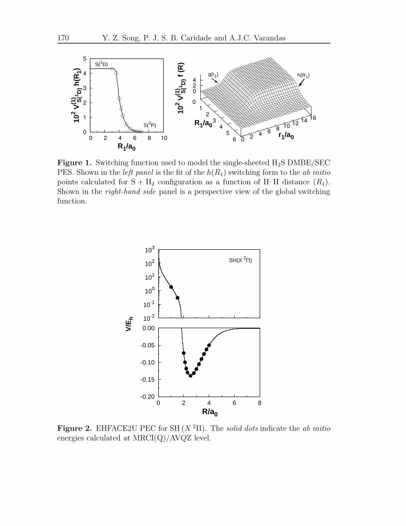
170 Y. Z. Song, P. J. S. B. Caridade and A.J.C. Varandas
0
1
2
3
4
5
0 2 4 6 8 10
102 V
(1) S(1 D
) h(R
1)
R1/a0
S(1D)
S(3P)
102 V
(1) S(1 D
) f(R
)
g(r1) h(R1)
0
1
2
3
4
5
6
R1/a0
02
46
810
1214
16
r1/a0
0
2
4
Figure 1. Switching function used to model the single-sheeted H2S DMBE/SECPES. Shown in the left panel is the fit of the h(R1) switching form to the ab initio
points calculated for S + H2 configuration as a function of H–H distance (R1).Shown in the right-hand side panel is a perspective view of the global switchingfunction.
-0.20
-0.15
-0.10
-0.05
0.00
0 2 4 6 8
V/E
h
R/a0
10-2
10-1
100
101
102
103
SH(X 2Π)
Figure 2. EHFACE2U PEC for SH (X 2Π). The solid dots indicate the ab initio
energies calculated at MRCI(Q)/AVQZ level.
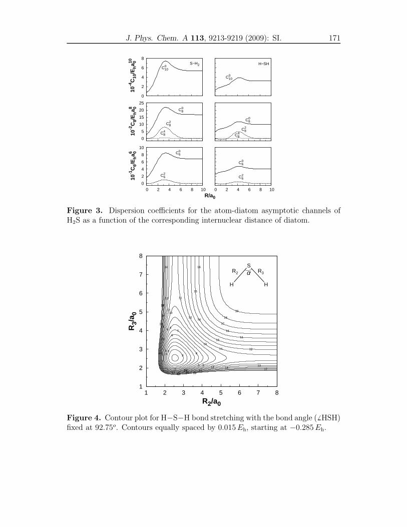
J. Phys. Chem. A 113, 9213-9219 (2009): SI. 171
0
2
4
6
8
10
0 2 4 6 8 10
10-1
C6/
Eha6 0
R/a0
C26
C06
0 2 4 6 8 10
C26
C06
0
5
10
15
20
25
10-2
C8/
Eha8 0
C48
C28
C08
C48
C28
C08
0
2
4
6
8
10-4
C10
/Eha10 0
C010
S−H2
C010
H−SH
Figure 3. Dispersion coefficients for the atom-diatom asymptotic channels ofH2S as a function of the corresponding internuclear distance of diatom.
1
2
3
4
5
6
7
8
1 2 3 4 5 6 7 8
R3/
a 0
R2/a0
19
19
19
18
18
18
17
17
17
17
16
16
16
16
15
15
15
15
14
14
14
14
13
13
13
13
12
12
12
12
11
11
11
11
10
10
10
9
9
8
8
7
7
6
6
5
4
3
2
H H
SR2 R3α
Figure 4. Contour plot for H−S−H bond stretching with the bond angle (6 HSH)fixed at 92.75o. Contours equally spaced by 0.015Eh, starting at −0.285Eh.


Chapter 7
Accurate DMBE/CBS PES forground-state HS2

J. Phys. Chem. A XXX, XXXX-XXXX (2011).
Accurate DMBE potential energy surface forground-state HS2 based on ab initio dataextrapolated to the complete basis set limit
Y. Z. Song and A.J.C. Varandas
Departamento de Quımica, Universidade de Coimbra
3004-535 Coimbra Codex, Portugal.
(Received: XXXX XX, 2011; Revised Manuscript Received: XXXX XX, 2011)
Abstract
A double many-body expansion potential energy surface is reported for the electronic
ground state of HS2 by fitting accurate multireference configuration interaction energies
calculated with aug-cc-pVTdZ and aug-cc-pVQdZ basis sets upon separate extrapola-
tion of the complete-active-space self-consistent field and dynamical correlation com-
ponents of the total energy to the complete basis set limit. The major topographical
features of the potential energy surface are examined in detail, and the model function
used for a thermalized calculation of the rate constants for the S + SH → H + S2 reac-
tion at 298 and 400K. A value of (1.44 ± 0.06) × 10−11cm3 s−1 at 298K is obtained,
providing perhaps the most reliable estimate of the rate constant known thus far for
such a reaction.
176 Y.Z. Song and A.J.C. Varandas
1 Introduction
The HS2 radical plays an important role in a variety of environments, notably
in combustion and the oxidation of reduced forms of sulfur.1–4 A vast amount
of investigation has been carried on HS2 both experimentally and theoretically
since the pioneering work by Porter5 who has first proposed that the HS2 radical
was produced during the photolysis of H2S2.
The first millimeter-wave spectra of HS2 reported by Yamamoto and Saito6
provided the first experimental information about the ground state structure of
HS2. Isoniemi et al.7 has subsequently investigated the infrared spectroscopy of
the HS2 radical in an Ar matrix following the 266 nm photolysis of H2S2. The
absorption bands for two vibrational motions of HS2 radical, namely the H-S
stretch and the HSS bend, are observed to be 2463 and 903 cm−1. In a recent
experiment, Ashworth and Fink8 have recorded the chemiluminescence spectrum
of the HS2 radical with a high-resolution Fouriertransform spectrometer. The
overview spectrum in the region between 4000 cm−1 and 9000 cm−1 has been
analyzed and the so obtained vibrational parameters presented.
Out of a vast theoretical work, Sannigrahi et al.9 pioneered the ab initio
calculations on the ground and excited states of HS2, which provided both struc-
tural and vibrational information. Owens et al.10 investigated HX2 radicals
(X = Al, Si, P, and S) using coupled cluster theory, CCSD(T), having reported
the equilibrium structure and vibrational frequencies at the global minimum.
Later, Denis11 reported more accurate structural and thermodynamic properties
of both ground and excited states of HS2 and HS+2 at the CCSD(T) and B3LYP
density functional levels of theory. Moreover, the structural and energetic prop-
erties of ground state HS2 and HSS → SSH transition state have been examined
using the CCSD(T) method by Francisco,12 who estimated the energy change
for the isomerization reaction to be of 31.7 ± 1 kcal mol−1. Quite recently, Peter-
son et al.13 calculated the equilibrium geometry of the ground and first excited
electronic states of HS2 with highly correlated coupled cluster methods followed
by basis set extrapolation. The centrifugal distortion constants, harmonic fre-
quencies, and vibration-rotation coupling constants have then been calculated
for both electronic states of HS2 and DS2 using accurate three-dimensional, near-
J. Phys. Chem. A XXX, XXXX-XXXX (2011). 177
equilibrium potential energy and dipole moment functions.
All the above studies have focused mainly on the structural and spectroscopic
constants of the HS2 radical at its global minimum. Indeed, as far as we are
aware, no work toward obtaining a global potential energy surface (PES) for
ground-state HS2(X 2A′′) has been reported thus far. In this work, we present
a realistic global PES for HS2(X 2A′′) based on double many-body expansion
(DMBE)14–17 theory by accurately fitting to the ab initio physically motivated
forms to the calculated ab initio energies once extrapolated to the complete basis
set (CBS) limit.
The paper is organized as follows. Section 2 describes the ab initio calculations
employed in the present work, while Section 3 provides a survey of the procedure
utilized to CBS extrapolate the calculated energies. The analytical modeling of
the DMBE/CBS PES is presented in Section 4. The major topographical features
of the resulting PES are discussed in section 5. Section 6 gathers the concluding
remarks.
2 Ab initio calculations
The ab initio calculations are carried out at the multi-reference configuration
interaction level18, 19 of theory, including the popular quasi-degenerate David-
son correction for quadruple excitations [MRCI(Q)],20 using the full-valence-
complete-active space (CASSCF21) wave function as reference (abbreviated as
CAS). All calculations are performed using the MOLPRO22 package. The stan-
dard aug-cc-pVXZ (AVXZ) basis set of Dunning23, 24 plus core-polarization high-
exponent d functions (AVXdZ)25 has been used for the S atom and AVXZ for
the H atoms, with X = T,Q. A grid of 1601 ab initio points have been cho-
sen to map the PES over the H − S2 region defined by 3.0 ≤ RS2/a0 ≤ 4.5,
2 ≤ rH−S2/a0 ≤ 10 and 0 ≤ γ/deg ≤ 90. For the S − SH interactions, a grid
defined by 2 ≤ RSH/a0 ≤ 4, 2 ≤ rS−SH/a0 ≤ 10 and 0 ≤ γ/deg ≤ 180 has been
chosen. For both channels, r, R and γ are the atom-diatom Jacobi coordinates.
178 Y.Z. Song and A.J.C. Varandas
3 Extrapolation to CBS limit
The ab initio energies calculated in this way have been subsequently extrapolated
to CBS limit. To perform the extrapolation, the MRCI(Q) energy is treated in
split form by writing26
EX(R) = ECASX (R) + Edc
X (R) (1)
where the subscript X indicates that the energy has been calculated in the
AVXdZ basis and the superscripts CAS and dc stand for complete-active-space
and dynamical correlation energies, respectively. Note that all extrapolations
are carried out pointwise, and hence, the vector R of the nuclear geometrical
coordinates will be omitted for simplicity.
To extrapolate the CAS (uncorrelated in the sense of lacking dynamical corre-
lation) energies, we have adopted the two-point extrapolation protocol proposed
by Karton and Martin (KM):27
ECASX = ECAS
∞ +B/Xα (2)
where α is an effective decay exponent. Being a two-parameter protocol (ECAS∞ , B),
a minimum of two raw energies will be required for the extrapolation. Specially,
Eq. (2) will be calibrated from the CAS/AV(T,Q)dZ energy pairs using a value
of α=5.34; note that this value has been found optimal when extrapolating HF
energies to the CBS limit, and has been suggested26 to be valid also for the CAS
energy.
To extrapolate the dynamic correlation (dc) energy, we utilize our own uni-
form singlet- and triplet-electron pair (USTE26, 28) scheme, which has already
been successfully utilized to construct global DMBE/CBS PESs of H2S(X 1A′)29
and NH2(1 2A′)30 (and partly also for ground-state H2O31 as well as jointly with
correlation scaling for the quartet ground-state of N332). It assumes the form.
EdcX = Edc
∞ +A3
(X + α)3+
A5
(X + α)5(3)
with A5 being determined by the auxiliary relation
A5 = A5(0) + cA5/43 (4)
J. Phys. Chem. A XXX, XXXX-XXXX (2011). 179
with A5(0) = 0.0037685459Eh, c = −1.17847713E−5/4h , and α = −3/8 are the
universal-type parameters. Thus, E∞ and A3 are the unknown to be determined
from a fit to the dc energies calculated with the AVTdZ and AVQdZ basis sets
[USTE(T,Q)]. Note that the USTE model suitably calibrated for a specific theory
has been shown26 to yield both the CBS extrapolated full correlation in systems
studied that by the popular single-reference Møller-Plesset (MP2) and coupled
cluster [CCSD and CCSD(T)] methods as well as its dynamical part in MRCI(Q)
calculations in very good agreement with the best available estimates. Since the
method has been described in detail in various papers ever since its proposal,
we refer the reader to Ref. [33] from which other references can be obtained by
cross-referencing.
4 Single-sheeted DMBE potential energy surface
Within the framework of DMBE14–17 theory, the single-sheeted PES is written as
V (R)=3∑
i=1
[V
(2)EHF(Ri) + V
(2)dc (Ri)
]+ V
(3)dc (R) + V
(3)ele (R) + V
(3)EHF(R) (5)
where R = {R1, R2, R3} is a collective diatomic internuclear separation of tri-
atomic, and the three-body electrostatic term (only present in the presence of
overlapping polarizable species) has been separated from the corresponding EHF
energy for clarity. Thus, the two-body energy terms are split into two contribu-
tions: the extended Hartree- Fock (EHF) and dynamical correlation (dc) energies.
Although a similar partition applies to all other n-body energy terms, the electro-
static (ele) long-range contribution has been separated for clarity as noted above,
since it varies at long-range with a form akin to three-body dynamical correlation
terms. The following subsections give a detailed description of the two-body and
three-body energy terms employed in Eq. (5).
4.1 Two-body energy terms
The diatomic potential energy curves of S2(X3Σ−
g ) and SH(X 2Π), have been
calibrated by fitting ab initio energies extrapolated as described in the previous
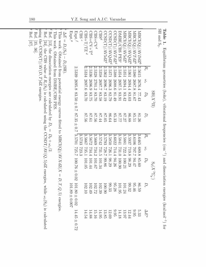
180 Y.Z. Song and A.J.C. Varandas
Table
1.
Equ
ilibriu
mgeom
etries(b
ohr),
vib
rational
frequ
encies
(cm−
1)an
dd
issociation
energies
(kcalmol −
1)for
SH
and
S2 .
SH
(X2Π
)S
2 (X3Σ
−g)
Re
ωe
D0
De
Re
ωe
D0
De
∆E
a
MR
CI(Q
)/AVD
dZ
b2.5615
2676.477.43
81.263.6465
689.885.60
86.595.33
MR
CI(Q
)/AVT
dZ
b2.5380
2687.881.67
85.513.6106
707.794.47
95.469.95
MR
CI(Q
)/AVQ
dZ
b2.5361
2694.483.03
86.883.5937
719.898.29
99.3212.44
MR
CI(Q
)/AV
5dZ
b2.5351
2694.183.42
87.273.5881
722.4100.21
101.2413.97
DM
BE
/CB
SP
ES
c2.5354
2697.583.91
87.773.5841
731.0100.90
101.9514.18
CC
SD
(T)/A
VT
dZ
d2.5388
2688.681.49
85.333.6022
714.494.26
95.289.95
CC
SD
(T)/A
VQ
dZ
d2.5371
2696.382.79
86.643.5850
726.198.29
99.3312.69
CC
SD
(T)/A
V5d
Zd
2.53622696.7
83.1987.05
3.5793728.7
99.86100.90
13.85C
BS
d2.5358
2697.783.58
87.443.5742
731.5101.34
102.3914.95
CB
S+
CV
d2.5328
2701.283.70
87.563.5669
734.2101.67
102.7215.16
CB
S+
CV
+T
d2.5336
2696.983.75
87.613.5672
734.4101.44
102.4914.88
CB
S+
T/T
Zd
2.53342697.6
83.7087.56
3.5667735.1
101.05102.10
14.54C
BS
e3.5733
723.3E
xp
t. f2.5339
2695.883.50±
0.787.35±
0.73.5701
725.7100.76±
0.02101.80±
0.0214.45±
0.72E
xp
t. g101.89±
0.007a
∆E
=D
e (S2 )−
De (S
H).
bT
his
work
.O
btain
edfrom
poten
tialen
ergycu
rvesfi
ttedto
MR
CI(Q
)/AVX
dZ
(X=D,T,Q,5)
energies.
cT
his
work
.O
btain
edfrom
DM
BE
/CB
SP
ES
.d
Ref.
[13],th
ed
issociation
energies
arecalcu
latedbyD
e=D
0+ω
e /2.e
Ref.
[34],th
eC
BS
value
ofR
e (S2 )
iscalcu
latedu
sing
the
CC
SD
T/A
V(Q,5)d
Zen
ergies,w
hile
ωe (S
2 )is
calculated
usin
gth
eC
CS
D(T
)/AV
(D,T
)dZ
energies.
fR
ef.[35,
36].g
Ref.
[37].
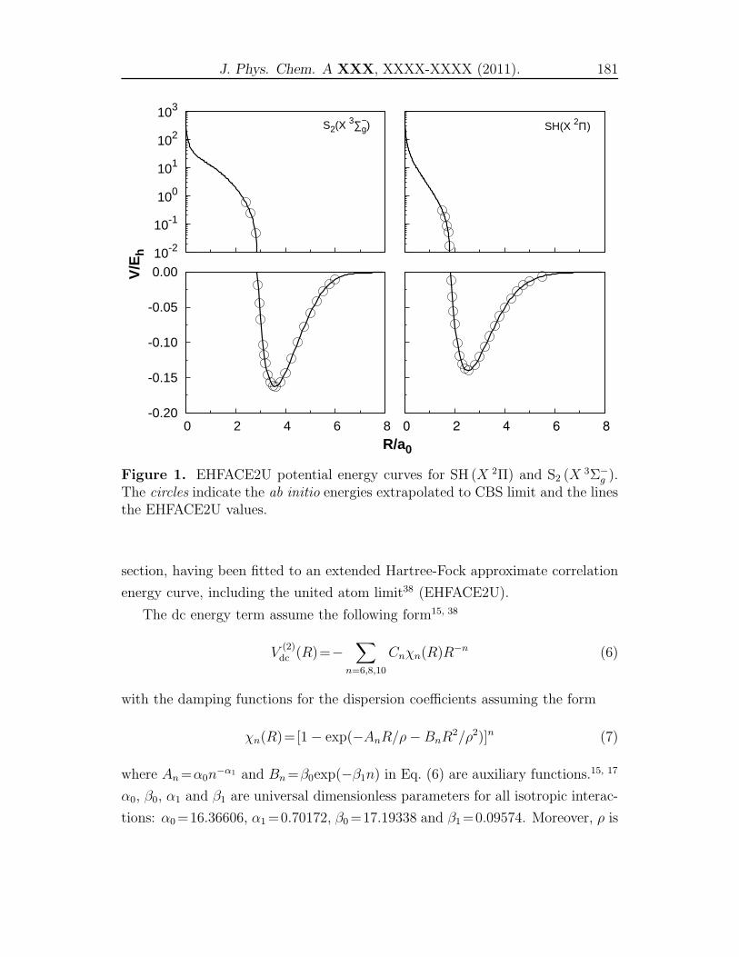
J. Phys. Chem. A XXX, XXXX-XXXX (2011). 181
SH(X 2Π)
10-2
10-1
100
101
102
103
S2(X 3∑−g)
-0.20
-0.15
-0.10
-0.05
0.00
0 2 4 6 8
V/E
h
R/a0
0 2 4 6 8
Figure 1. EHFACE2U potential energy curves for SH (X 2Π) and S2 (X 3Σ−g ).
The circles indicate the ab initio energies extrapolated to CBS limit and the linesthe EHFACE2U values.
section, having been fitted to an extended Hartree-Fock approximate correlation
energy curve, including the united atom limit38 (EHFACE2U).
The dc energy term assume the following form15, 38
V(2)dc (R)=−
∑
n=6,8,10
Cnχn(R)R−n (6)
with the damping functions for the dispersion coefficients assuming the form
χn(R)=[1 − exp(−AnR/ρ−BnR2/ρ2)]n (7)
where An =α0n−α1 and Bn =β0exp(−β1n) in Eq. (6) are auxiliary functions.15, 17
α0, β0, α1 and β1 are universal dimensionless parameters for all isotropic interac-
tions: α0 =16.36606, α1 =0.70172, β0 =17.19338 and β1 =0.09574. Moreover, ρ is
182 Y.Z. Song and A.J.C. Varandas
a scaling parameter defined by ρ/a0 =5.5+1.25R0, where R0 =2(〈r2X〉1/2+〈r2
Y 〉1/2)
is the LeRoy39 parameter, and 〈r2X〉 is the expectation value of squared radius for
the outermost electron in atom X (X=A,B).
The exponential decaying portion of the EHF-type energy term is written as
V(2)EHF(R) = −D
R
(1 +
5∑
i=1
airi
)exp(−γ r) (8)
where
γ = γ0[1 + γ1tan(γ2r)] (9)
r = R − Re is the displacement from the equilibrium diatomic geometry; D,
ai(i = 1, · · · , n) and γi in Eq. (8) are adjustable parameters to be obtained as
described elsewhere.15, 38
The numerical values of all the parameters for both diatomic potentials are
gathered in Table 1 of the Supporting Information, while their internuclear depen-
dences are shown in Figure 1. As seen, the modeled potentials mimic accurately
the ab initio energies. Equilibrium geometry, vibrational frequencies and dissocia-
tion energy are collected in Table 1. For both S2 and SH, the dissociation energies
increase monotonously as the size of basis sets increasing from AVDdZ to AV5dZ
and the DMBE/CBS PES gives the deepest well depth. Comparing with the CBS
results by Peterson et al.13 which are extrapolated using CCSD(T)/AV(Q, 5)dZ
energies, our results for the SH diatomic predict a difference of 0.0004 a0 in the
equilibrium geometry, give vibrational frequencies 0.2 cm−1 smaller and dissoci-
ation energies only 0.33 kcal mol−1 smaller. For the S2 diatom, the variations
are 0.0099 a0, 0.5 cm−1 and 0.44 kcal mol−1, respectively. This may be considered
quite good since we have avoided any expensive MRCI(Q)/AV5dZ calculations.
Comparing with the experimental values, our results also provide an excellent
agreement. Table 1 also shows the difference of SH and S2 dissociation energies
[De(S2)−De(SH)]. The first observation goes to the AVDdZ result which as might
be expected is poor, with the AVTdZ result still giving an error of more than
4 kcal mol−1 when comparing with the experimental value. Naturally, the AVQdZ
and AV5dZ results show enhanced agreement with experiment, with differences of
2.01 kcal mol−1 and 0.48 kcal mol−1, respectively. Notably, the DMBE/CBS PES
predicts a value of 14.18 kcal mol−1, which differs by 0.77 kcal mol−1 from the CBS
J. Phys. Chem. A XXX, XXXX-XXXX (2011). 183
results by Peterson et al.13 and 0.27 kcal mol−1 from the experimental value.
4.2 Three-Body Energy Terms
4.2.1 Three-body Dynamical Correlation Energy
The three-body dynamical correlation energy assumes the usual form of a sum-
mation in inverse powers of the fragment separation distances:40
V(3)dc = −
3∑
i=1
∑
n
fi(R)χn(ri)C(i)n (Ri, θi)r
−ni (10)
where the first summation includes all atom-diatom interactions (i ≡ A − BC).
Ri is the diatomic internuclear distance, ri is the separation between atom A and
the center-of-mass of the BC diatomic internuclear coordinate, and θi is the angle
between these two vectors (see Figure 1 of Ref. 41). fi = 12{1 − tanh[ξ(ηRi −
Rj − Rk)]} is a convenient switching function, where we have fixed η = 6 and
ξ = 0.6 a−10 ; corresponding expressions apply to Rj , Rk, fj, and fk. χn(ri) is
the damping function, which still takes the forms in Eq. (7), but replace R by
the center-of-mass separation for the relevant atom-diatom channel. The atom-
diatom dispersion coefficients in Eq. (10) is given by
C(i)n =
∑
L
CLnPL(cosθi) (11)
where PL(cosθi) denotes the L-th term of Legendre polynomial expansion and CLn
is the associated expansion coefficient. The expansion in Eq. (11) has been trun-
cated by considering only the coefficients C06 , C
26 , C
08 , C
28 , C
48 , and C0
10; all other
coefficients have been assumed to make a negligible contribution, and hence ne-
glected. To estimate the dispersion coefficients, we have utilized the generalized
Slater-Kirkwood approximation.42 As usual, the atom-diatom dispersion coeffi-
cients so calculated for a set of nuclear distances have then been fitted to the
form
CL,A−BCn (R) = CL,AB
n + CL,ACn +DM(1 +
3∑
i=1
airi)exp(−
3∑
i=1
biri) (12)
where r = R − RM is the displacement relative to the position of the maximum
and b1 = a1. CL,ABn , for L = 0, are the corresponding atom-atom dispersion
184 Y.Z. Song and A.J.C. Varandas
coefficients(for L 6= 0, CL,ABn = 0). The least-squares parameters that result
from such fits are collected in Table 2 of the Supporting Information, while their
internuclear dependences are displayed in Figure 1 of the Supporting Information.
Note that, for R = 0, the isotropic component of the dispersion coefficient is fixed
at the corresponding value in the A–X pair, where X represents the united atom
of BC at the limit of a vanishingly small internuclear separation. As pointed
out elsewhere,40 Eq. (10) causes an overestimation of the dynamical correlation
energy at the atom-diatom dissociation channel. To correct such a behavior, we
have multiplied the two-body dynamical correlation energy for i-pair by Πj 6=i(1−fj), correspondingly for channels j and k. This ensures that the only two-body
contribution at the i-th channel is that of BC.
4.2.2 Three-body electrostatic energy
Since the H atom has spherical symmetry, the long-range electrostatic potential
terms of HS2 only arise from the interaction of the permanent quadrupole moment
of the sulfur atom with the permanent dipole and quadruple moments of SH
diatom. Following the previous work43–45 , the electrostatic energy is written as
V(3)ele = f(R){C4(R, r)ADQ(θa, θ, φab))r−4 + C5(R, r)AQQ(θa, θ, φab))r−5} (13)
where the f(R), R, r and θ have the same meaning as in Section 4.2.1, the
θa is the angle that defines the atomic quadrupole orientation, and φab is the
corresponding dihedral angle. The coefficients C4(R, r) and C5(R, r) are given by
C4(R, r) =3
2QSDSH(R)χ4(r)
C5(R, r) =3
4QSQSH(R)χ5(r) (14)
where the DSH(R) and QSH(R) are the permanent electric dipole and quadru-
ple moments of SH, and QS is the quadruple moment of the sulfur atom. The
functional form of the angular variations of ADQ and AQQ take the expressions em-
ployed in previous work?, 45, 46 based on the classical-optimized-quadruple (COQ)
model.47–51
The analytical expression for the SH dipole has been obtained by fitting our
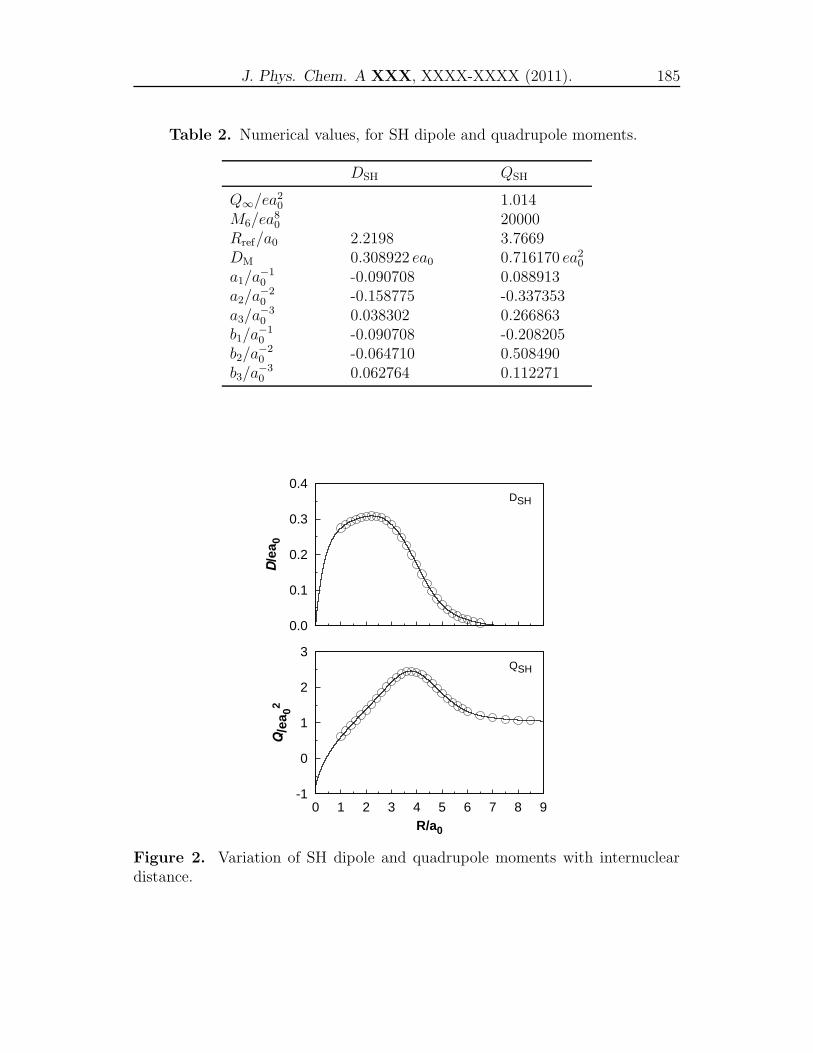
J. Phys. Chem. A XXX, XXXX-XXXX (2011). 185
Table 2. Numerical values, for SH dipole and quadrupole moments.
DSH QSH
Q∞/ea20 1.014
M6/ea80 20000
Rref/a0 2.2198 3.7669DM 0.308922 ea0 0.716170 ea2
0
a1/a−10 -0.090708 0.088913
a2/a−20 -0.158775 -0.337353
a3/a−30 0.038302 0.266863
b1/a−10 -0.090708 -0.208205
b2/a−20 -0.064710 0.508490
b3/a−30 0.062764 0.112271
0.0
0.1
0.2
0.3
0.4
D/e
a 0
DSH
-1
0
1
2
3
0 1 2 3 4 5 6 7 8 9
Q/e
a 02
R/a0
QSH
Figure 2. Variation of SH dipole and quadrupole moments with internucleardistance.
186 Y.Z. Song and A.J.C. Varandas
own ab initio results to the form52
D(R) = DM(1 +
3∑
i=1
ai ri) exp(−
3∑
i=1
bi ri) (15)
where r = R−Rref and Rref is the reference distance corresponding to the maxi-
mum in the D(R) curve, and b1 ≡ a1. In turn, the variation of the SH quadrupole
moment with the internuclear distance has been fitted to the following model51
Q(R) = DM(1 +
3∑
i=1
ai ri) exp(−
3∑
i=1
bi ri) +Q∞ + χ8(R)
M6
R6(16)
where r = R − Rref with Rref being the reference distance corresponding to the
maximum in the Q(R) curve. Q∞ is the value of the separated-atoms quadrupole
limit. The parameters in Eq. (15) and (16) are collected in Table 2, while their
graphical view of the modeled functions can be seen in Figure 2.
4.2.3 Three-body extended Hartree-Fock energy
By removing, for a given triatomic geometry, the sum of the two-body energy
terms from the corresponding DMBE interaction energies Eq. (5), which was de-
fined with respect to the infinitely separated ground-state atoms, one obtains
the total three-body energy. Then by subtracting the three-body dynamical cor-
relation contribution Eq. (10) and the three-body electrostatic energy Eq. (13)
from the total three-body energy, one obtains the three-body extended Hartree-
Fock energy. This can be represented by the following three-body distributed-
polynomial45 form
V(3)EHF =
3∑
j=1
P j(Q1, Q2, Q3) ×3∏
i=1
{1 − tanh[γji (Ri − Rj,ref
i )]} (17)
where P j(Q1, Q2, Q3) is the j-th polynomial up to six-order in the symmetry
coordinates. As usual, we obtain the reference geometries Rj,refi by first assuming
their values to coincide with bond distances of the associated stationary points.
Subsequently, we relax this condition via a trial-and-error least-squares fitting
procedure. Similarly, the nonlinear range-determining parameters γji have been
optimized in this way. The complete set of parameters amounts to a total of 150
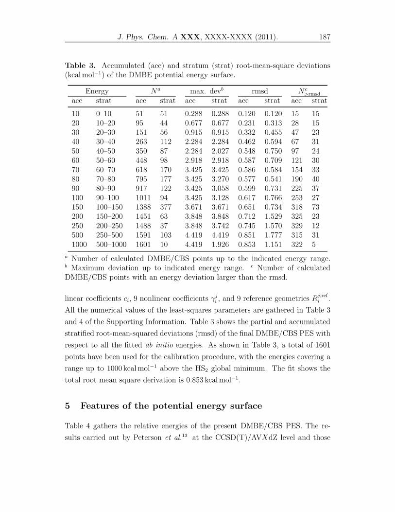
J. Phys. Chem. A XXX, XXXX-XXXX (2011). 187
Table 3. Accumulated (acc) and stratum (strat) root-mean-square deviations(kcal mol−1) of the DMBE potential energy surface.
Energy Na max. devb rmsd N c>rmsd
acc strat acc strat acc strat acc strat acc strat
10 0–10 51 51 0.288 0.288 0.120 0.120 15 1520 10–20 95 44 0.677 0.677 0.231 0.313 28 1530 20–30 151 56 0.915 0.915 0.332 0.455 47 2340 30–40 263 112 2.284 2.284 0.462 0.594 67 3150 40–50 350 87 2.284 2.027 0.548 0.750 97 2460 50–60 448 98 2.918 2.918 0.587 0.709 121 3070 60–70 618 170 3.425 3.425 0.586 0.584 154 3380 70–80 795 177 3.425 3.270 0.577 0.541 190 4090 80–90 917 122 3.425 3.058 0.599 0.731 225 37100 90–100 1011 94 3.425 3.128 0.617 0.766 253 27150 100–150 1388 377 3.671 3.671 0.651 0.734 318 73200 150–200 1451 63 3.848 3.848 0.712 1.529 325 23250 200–250 1488 37 3.848 3.742 0.745 1.570 329 12500 250–500 1591 103 4.419 4.419 0.851 1.777 315 311000 500–1000 1601 10 4.419 1.926 0.853 1.151 322 5
a Number of calculated DMBE/CBS points up to the indicated energy range.b Maximum deviation up to indicated energy range. c Number of calculatedDMBE/CBS points with an energy deviation larger than the rmsd.
linear coefficients ci, 9 nonlinear coefficients γji , and 9 reference geometries Rj,ref
i .
All the numerical values of the least-squares parameters are gathered in Table 3
and 4 of the Supporting Information. Table 3 shows the partial and accumulated
stratified root-mean-squared deviations (rmsd) of the final DMBE/CBS PES with
respect to all the fitted ab initio energies. As shown in Table 3, a total of 1601
points have been used for the calibration procedure, with the energies covering a
range up to 1000 kcal mol−1 above the HS2 global minimum. The fit shows the
total root mean square derivation is 0.853 kcal mol−1.
5 Features of the potential energy surface
Table 4 gathers the relative energies of the present DMBE/CBS PES. The re-
sults carried out by Peterson et al.13 at the CCSD(T)/AVXdZ level and those
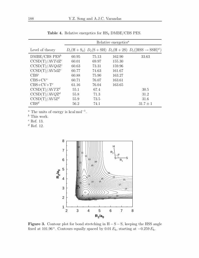
188 Y.Z. Song and A.J.C. Varandas
Table 4. Relative energetics for HS2 DMBE/CBS PES.
Relative energeticsa
Level of theory De(H + S2) De(S + SH) De(H + 2S) De([HSS → SSH]6=)
DMBE/CBS PESb 60.95 75.13 162.90 33.63CCSD(T)/AVTdZc 60.01 69.97 155.30CCSD(T)/AVQdZc 60.63 73.31 159.96CCSD(T)/AV5dZc 60.77 74.63 161.67CBSc 60.88 75.90 163.27CBS+CVc 60.71 76.07 163.61CBS+CV+Tc 61.16 76.04 163.65CCSD(T)/AVTZd 55.1 67.4 30.5CCSD(T)/AVQZd 55.8 71.3 31.2CCSD(T)/AV5Zd 55.9 73.5 31.6CBSd 56.2 74.1 31.7 ± 1
a The units of energy is kcal mol−1.b This work.c Ref. 13.d Ref. 12.
1
2
3
4
5
6
7
8
2 3 4 5 6 7 8
R2/
a 0
R1/a0
24
67
8
9
9 10
11
11
11
12
12
13
13
13
14
1414
15
15
15
16
17
1717
18
18
18
19
19
21
2121
22
22 22
23
23
23
H
S S
R2
R1
α
Figure 3. Contour plot for bond stretching in H− S− S, keeping the HSS anglefixed at 101.96 o. Contours equally spaced by 0.01Eh, starting at −0.259Eh.
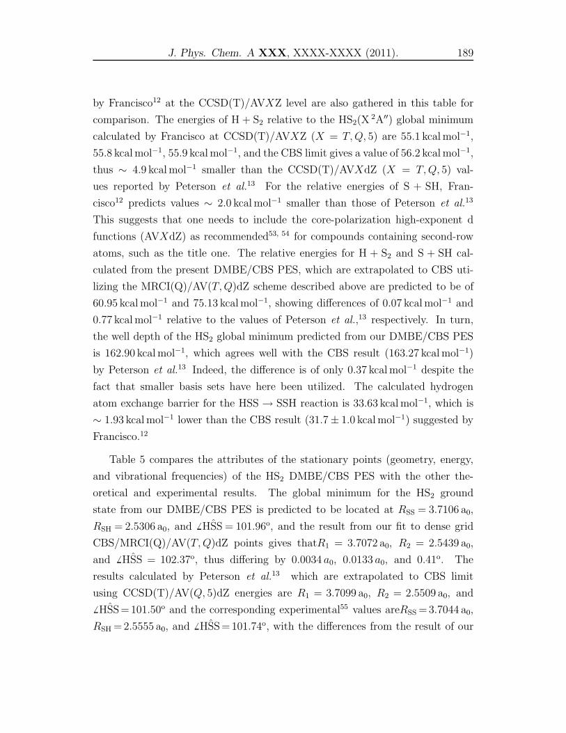
J. Phys. Chem. A XXX, XXXX-XXXX (2011). 189
by Francisco12 at the CCSD(T)/AVXZ level are also gathered in this table for
comparison. The energies of H + S2 relative to the HS2(X2A′′) global minimum
calculated by Francisco at CCSD(T)/AVXZ (X = T,Q, 5) are 55.1 kcal mol−1,
55.8 kcal mol−1, 55.9 kcal mol−1, and the CBS limit gives a value of 56.2 kcal mol−1,
thus ∼ 4.9 kcal mol−1 smaller than the CCSD(T)/AVXdZ (X = T,Q, 5) val-
ues reported by Peterson et al.13 For the relative energies of S + SH, Fran-
cisco12 predicts values ∼ 2.0 kcal mol−1 smaller than those of Peterson et al.13
This suggests that one needs to include the core-polarization high-exponent d
functions (AVXdZ) as recommended53, 54 for compounds containing second-row
atoms, such as the title one. The relative energies for H + S2 and S + SH cal-
culated from the present DMBE/CBS PES, which are extrapolated to CBS uti-
lizing the MRCI(Q)/AV(T,Q)dZ scheme described above are predicted to be of
60.95 kcal mol−1 and 75.13 kcal mol−1, showing differences of 0.07 kcal mol−1 and
0.77 kcal mol−1 relative to the values of Peterson et al.,13 respectively. In turn,
the well depth of the HS2 global minimum predicted from our DMBE/CBS PES
is 162.90 kcal mol−1, which agrees well with the CBS result (163.27 kcal mol−1)
by Peterson et al.13 Indeed, the difference is of only 0.37 kcal mol−1 despite the
fact that smaller basis sets have here been utilized. The calculated hydrogen
atom exchange barrier for the HSS → SSH reaction is 33.63 kcal mol−1, which is
∼ 1.93 kcal mol−1 lower than the CBS result (31.7 ± 1.0 kcal mol−1) suggested by
Francisco.12
Table 5 compares the attributes of the stationary points (geometry, energy,
and vibrational frequencies) of the HS2 DMBE/CBS PES with the other the-
oretical and experimental results. The global minimum for the HS2 ground
state from our DMBE/CBS PES is predicted to be located at RSS = 3.7106 a0,
RSH = 2.5306 a0, and 6 HSS = 101.96o, and the result from our fit to dense grid
CBS/MRCI(Q)/AV(T,Q)dZ points gives thatR1 = 3.7072 a0, R2 = 2.5439 a0,
and 6 HSS = 102.37o, thus differing by 0.0034 a0, 0.0133 a0, and 0.41o. The
results calculated by Peterson et al.13 which are extrapolated to CBS limit
using CCSD(T)/AV(Q, 5)dZ energies are R1 = 3.7099 a0, R2 = 2.5509 a0, and
6 HSS = 101.50o and the corresponding experimental55 values areRSS = 3.7044 a0,
RSH = 2.5555 a0, and 6 HSS = 101.74o, with the differences from the result of our
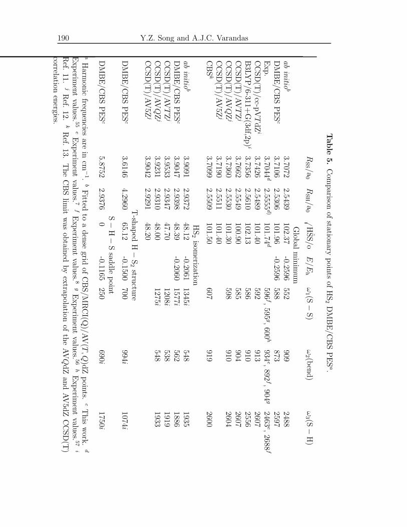
190 Y.Z. Song and A.J.C. Varandas
Table
5.
Com
parison
ofstation
aryp
oints
ofH
S2
DM
BE
/CB
SP
ES
a.
RSS /a
0R
SH/a
06
HS
S/o
E/E
hω
1 (S−
S)
ω2 (b
end
)ω
3 (S−
H)
Glob
alm
inim
um
ab
initio
b3.7072
2.5439102.37
-0.2596552
9092488
DM
BE
/CB
SP
ES
c3.7106
2.5306101.96
-0.2596588
8732597
Exp
.3.7044
d2.5555
d)
101.74d
596f,
595g,
600h
934e,
892f,
904g
2463e,
2688f
CC
SD
(T)/cc-p
VT
dZ
i3.7426
2.5489101.40
592913
2607B
3LY
P/6-311+
G(3d
f,2p)i
3.73562.5610
102.13586
9102556
CC
SD
(T)/A
VT
Zj
3.76622.5549
100.90585
9042607
CC
SD
(T)/A
VQ
Zj
3.73602.5530
101.30598
9102604
CC
SD
(T)/A
V5Z
j3.7190
2.5511101.40
CB
Sk
3.70992.5509
101.50607
9192600
HS
2isom
erizationab
initio
b3.9091
2.937248.12
-0.20611345i
5481935
DM
BE
/CB
SP
ES
c3.9047
2.939848.39
-0.20601577i
5621886
CC
SD
(T)/A
VT
Zj
3.95332.9347
47.701208i
5381919
CC
SD
(T)/A
VQ
Zj
3.92312.9310
48.001275i
5481933
CC
SD
(T)/A
V5Z
j3.9042
2.929148.20
T-sh
aped
H−
S2
structu
reD
MB
E/C
BS
PE
Sc
3.61464.2960
65.12-0.1500
700994i
1074i
S−
H−
Ssad
dle
poin
tD
MB
E/C
BS
PE
Sc
5.87522.9376
0-0.1165
250690i
1750i
aH
armon
icfreq
uen
ciesare
incm
−1.
bF
ittedto
ad
ense
gridof
CB
S/M
RC
I(Q)/A
V(T,Q
)dZ
poin
ts.c
Th
isw
ork.
d
Exp
erimen
tvalu
es. 55
eE
xp
erimen
tvalu
es. 7f
Exp
erimen
tvalu
es. 8g
Exp
erimen
tvalu
es. 56
hE
xp
erimen
tvalu
es. 57
i
Ref.
11.j
Ref.
12.k
Ref.
13.T
he
CB
Slim
itw
asob
tained
by
extrap
olationof
the
AVQ
dZ
and
AV
5dZ
CC
SD
(T)
correlationen
ergies.
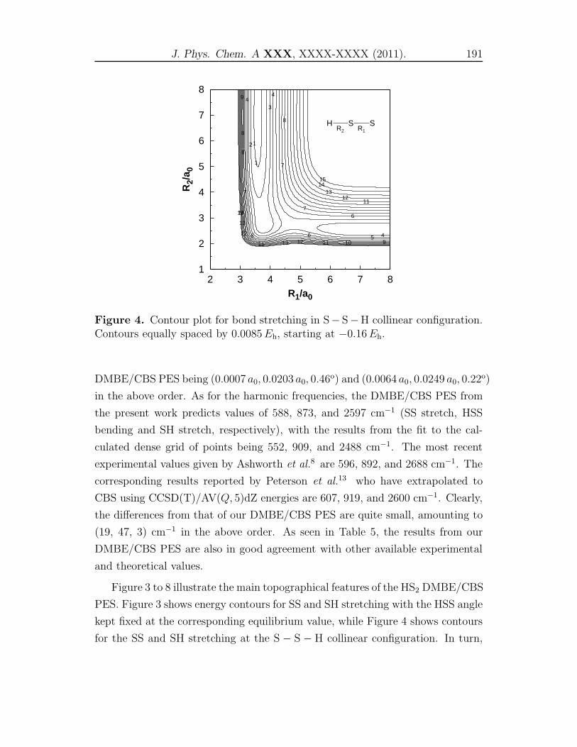
J. Phys. Chem. A XXX, XXXX-XXXX (2011). 191
1
2
3
4
5
6
7
8
2 3 4 5 6 7 8
R2/
a 0
R1/a0
1
1
2
34
4
45
6
6 6
7
7
7
8
8
8
9
910
11
11 11
12
12
12
13
13
13
14
14
15
15
H S SR2 R1
Figure 4. Contour plot for bond stretching in S− S−H collinear configuration.Contours equally spaced by 0.0085Eh, starting at −0.16Eh.
DMBE/CBS PES being (0.0007 a0, 0.0203 a0, 0.46o) and (0.0064 a0, 0.0249 a0, 0.22o)
in the above order. As for the harmonic frequencies, the DMBE/CBS PES from
the present work predicts values of 588, 873, and 2597 cm−1 (SS stretch, HSS
bending and SH stretch, respectively), with the results from the fit to the cal-
culated dense grid of points being 552, 909, and 2488 cm−1. The most recent
experimental values given by Ashworth et al.8 are 596, 892, and 2688 cm−1. The
corresponding results reported by Peterson et al.13 who have extrapolated to
CBS using CCSD(T)/AV(Q, 5)dZ energies are 607, 919, and 2600 cm−1. Clearly,
the differences from that of our DMBE/CBS PES are quite small, amounting to
(19, 47, 3) cm−1 in the above order. As seen in Table 5, the results from our
DMBE/CBS PES are also in good agreement with other available experimental
and theoretical values.
Figure 3 to 8 illustrate the main topographical features of the HS2 DMBE/CBS
PES. Figure 3 shows energy contours for SS and SH stretching with the HSS angle
kept fixed at the corresponding equilibrium value, while Figure 4 shows contours
for the SS and SH stretching at the S − S − H collinear configuration. In turn,
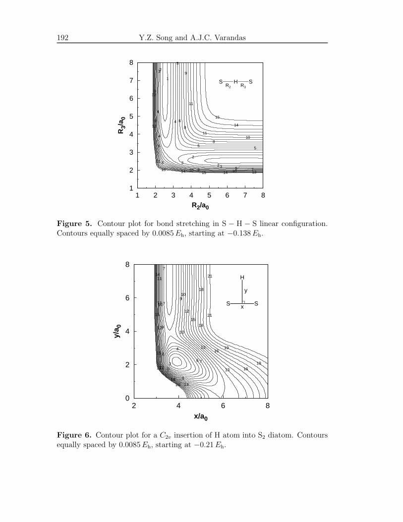
192 Y.Z. Song and A.J.C. Varandas
1
2
3
4
5
6
7
8
1 2 3 4 5 6 7 8
R3/
a 0
R2/a0
1
2
2
2
3
33
4
4
4
5
5
5
6
66
7
8
8
8
8
9
9
9
10
10 10
11
11
11
12
12
13
14
14 14
15
1515
S H SR2 R3
Figure 5. Contour plot for bond stretching in S − H − S linear configuration.Contours equally spaced by 0.0085Eh, starting at −0.138Eh.
0
2
4
6
8
2 4 6 8
y/a 0
x/a0
2
4
5
6 7
7
7
8
8
9
910
10
10
11
11
12
12
12
13
13
13
14
15
15
15
16
16
16
18
18
19
19
19
20
21
21
S S
H
x
y
Figure 6. Contour plot for a C2v insertion of H atom into S2 diatom. Contoursequally spaced by 0.0085Eh, starting at −0.21Eh.
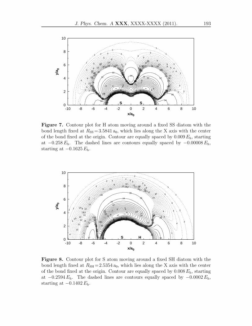
J. Phys. Chem. A XXX, XXXX-XXXX (2011). 193
0
2
4
6
8
10
-10 -8 -6 -4 -2 0 2 4 6 8 10
y/a 0
x/a0
S S
3
3
4
45
5
6
67
7
7
8
88
99
910
10 10
11
11
1111
12
12
12
12
12
13
1313
13
14
14
14
14
15
161617
17
1818
19
20
20
21 2222
23
24
24 25
1
1
1
1
1
1
1
1
1
2
2
22
2
2
2
2
2
2
3
3
333
3
3
33
4
4
44
4
4
44
5
5
5
5
55
5
6
6
6
6
6
6
66
7
7
7
7
7
77
8
8
8
8
8
8
8
9
9
9
9
99
10
10
10
10
10 10
11
11
11
11
1111
12
1212
12
12
12
131313
13
13 13
14
14
14
14 14
14
15
15
15
15
1515
16
16
16
16
16
16
17
17
17
17
17
17
18
1818
18
18 18
19
19
19
19 19
19
202020
20 20
21
2121
21
21
21
22
22
22
22
22
22
23
2323
23
23
23
2424
24
2424
252525
25
25
25
26
2626
26
26
26
272727
27 27
2828
28
28 28
29
29
29
29
29
3030
3030
30
Figure 7. Contour plot for H atom moving around a fixed SS diatom with thebond length fixed at RSS =3.5841 a0, which lies along the X axis with the centerof the bond fixed at the origin. Contour are equally spaced by 0.009Eh, startingat −0.258Eh. The dashed lines are contours equally spaced by −0.00008Eh,starting at −0.1625Eh.
0
2
4
6
8
10
-10 -8 -6 -4 -2 0 2 4 6 8 10
y/a 0
x/a0
S H
34
45
5
66 77
8
8
8
9
99
1010
10
11
11
11
12
12
12
13
13 13
14
14
14 14
15
15
15
15
15
1616
16
16
1617
17
17
18
18
18
19
19
20
20
21
21222323 24
24
25
25
25
26
1
1 1
1
1
1
1
1
2
2
2
2
2
2
2
3
3
3
3
3
3
3
4
4 4
4
44
4
4
5
5
55
55
5
5
6 6
6
6
6
6
67 7
7
7
8
88
8
8
8
8
9
9
9
9
9
9
10
10
10
1010
10
10
11
1111
11
11
11
11
11
12 12
12
12
12
12 13 13
13
13
13
13
14
14
14
14
14
14
1515
1515
15
1616
1616
16
16
17 17
17
17
17
17
18
18
Figure 8. Contour plot for S atom moving around a fixed SH diatom with thebond length fixed at RSH =2.5354 a0, which lies along the X axis with the centerof the bond fixed at the origin. Contour are equally spaced by 0.008Eh, startingat −0.2594Eh. The dashed lines are contours equally spaced by −0.0002Eh,starting at −0.1402Eh.
194 Y.Z. Song and A.J.C. Varandas
Figure 5 shows a contour plot for the stretching of the two SH bonds at a S−H−S
linear configuration. The notable features from Figure 5 are the two equivalent
asymmetric hydrogen bonded minima which are separated by a barrier lying half
way between them. The location of the barrier is found to be RSS =5.8752 a0 and
RSH = 2.9376 a0, with the harmonic frequencies at the top being 250, 690i, and
1750i cm−1, respectively.
Figure 6 shows a contour plot for the C2v insertion of H into the S2 diatomic.
The important features from this Figure are the saddle point structure for the
HSS → SSH isomerization (see text before) and the barrier for the H + S2 reac-
tion. The saddle point for isomerization is found to be located at RSS =3.9047 a0,
RSH =2.9398 a0, and 6 HSS=48.39o, with the barrier height lying at −0.2060Eh,
and the harmonic frequencies being 1577i, 562, and 1886 cm−1. Comparing
with the results of Francisco,12 the agreement is good. The barrier is located
at RSS = 3.6146 a0 and RSH = 4.2960 a0, with the well depth being −0.1500Eh.
The vibrational frequencies are also gathered in Table 5.
Figure 7 shows a contour plot for a H atom moving around a SS diatom
with the bond length fixed at RSS = 3.5841 a0, which lies along the X-axis with
the center of the bond fixed at the origin. The two salient features are the deep
minima connected by a C2v saddle point which allows scrambling of the two sulfur
atoms. Also visible along the C2v line is a closed contour apparently showing a
maximum. It is indeed a conical intersection that is undescribable within the
present single-sheeted DMBE formalism. In turn, Figure 8 shows a contour plot
for S atom moving around a fixed SH diatom with the bond length fixed at
RSH =2.5354 a0, which lies along the X-axis with the center of the bond fixed at
the origin. The two plots clearly reveal a smooth behavior both at short and long
range regions.
Shown in Figures 9 and 10 are the spherically averaged isotropic (V0) and lead-
ing anisotropic potentials for H + S2(V2) and S + SH(V1, V2) scattering processes
with the diatom fixed at its equilibrium geometry. Note that the magnitude of
the isotropic average potential V0 determines how close on average the atom and
molecule can approach each other, while the sign of V2 indicates whether or not
the molecule prefers to orient its axis along the direction of the incoming atom:
a negative value favors the collinear approach while a positive value favors the
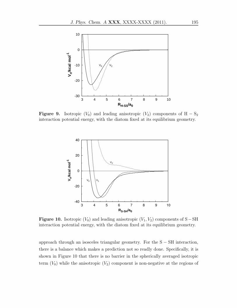
J. Phys. Chem. A XXX, XXXX-XXXX (2011). 195
-30
-20
-10
0
10
3 4 5 6 7 8 9 10
Vn/k
cal
mo
l-1
RH-SS/a0
V2V0
Figure 9. Isotropic (V0) and leading anisotropic (V2) components of H − S2
interaction potential energy, with the diatom fixed at its equilibrium geometry.
-40
-20
0
20
40
3 4 5 6 7 8 9 10
Vn/k
cal m
ol-1
RS-SH/a0
V2
V0 V1
Figure 10. Isotropic (V0) and leading anisotropic (V1, V2) components of S−SHinteraction potential energy, with the diatom fixed at its equilibrium geometry.
approach through an isosceles triangular geometry. For the S − SH interaction,
there is a balance which makes a prediction not so readly done. Specifically, it is
shown in Figure 10 that there is no barrier in the spherically averaged isotropic
term (V0) while the anisotropic (V2) component is non-negative at the regions of
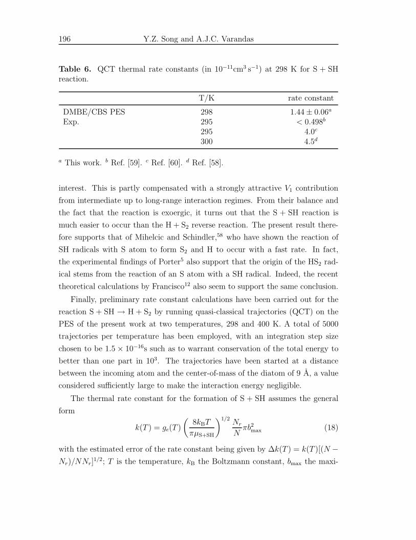
196 Y.Z. Song and A.J.C. Varandas
Table 6. QCT thermal rate constants (in 10−11cm3 s−1) at 298 K for S + SHreaction.
T/K rate constant
DMBE/CBS PES 298 1.44 ± 0.06a
Exp. 295 < 0.498b
295 4.0c
300 4.5d
a This work. b Ref. [59]. c Ref. [60]. d Ref. [58].
interest. This is partly compensated with a strongly attractive V1 contribution
from intermediate up to long-range interaction regimes. From their balance and
the fact that the reaction is exoergic, it turns out that the S + SH reaction is
much easier to occur than the H + S2 reverse reaction. The present result there-
fore supports that of Mihelcic and Schindler,58 who have shown the reaction of
SH radicals with S atom to form S2 and H to occur with a fast rate. In fact,
the experimental findings of Porter5 also support that the origin of the HS2 rad-
ical stems from the reaction of an S atom with a SH radical. Indeed, the recent
theoretical calculations by Francisco12 also seem to support the same conclusion.
Finally, preliminary rate constant calculations have been carried out for the
reaction S + SH → H + S2 by running quasi-classical trajectories (QCT) on the
PES of the present work at two temperatures, 298 and 400 K. A total of 5000
trajectories per temperature has been employed, with an integration step size
chosen to be 1.5 × 10⁻¹⁶s such as to warrant conservation of the total energy to
better than one part in 103. The trajectories have been started at a distance
between the incoming atom and the center-of-mass of the diatom of 9 A, a value
considered sufficiently large to make the interaction energy negligible.
The thermal rate constant for the formation of S + SH assumes the general
form
k(T ) = ge(T )
(8kBT
πµS+SH
)1/2Nr
Nπb2max (18)
with the estimated error of the rate constant being given by ∆k(T ) = k(T )[(N −Nr)/NNr]
1/2; T is the temperature, kB the Boltzmann constant, bmax the maxi-
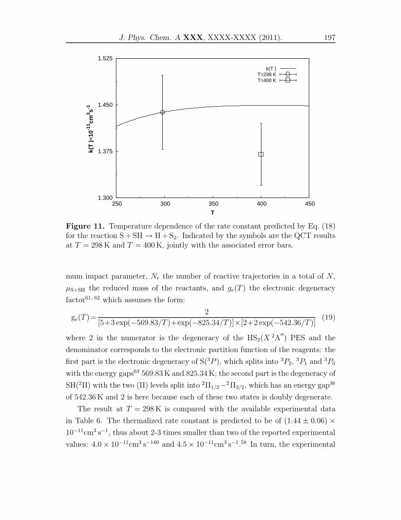
J. Phys. Chem. A XXX, XXXX-XXXX (2011). 197
1.300
1.375
1.450
1.525
250 300 350 400 450
k(T
)×1
0-11 cm
3 s-1
T
k(T )T=298 KT=400 K
Figure 11. Temperature dependence of the rate constant predicted by Eq. (18)for the reaction S + SH → H + S2. Indicated by the symbols are the QCT resultsat T = 298 K and T = 400 K, jointly with the associated error bars.
mum impact parameter, Nr the number of reactive trajectories in a total of N ,
µS+SH the reduced mass of the reactants, and ge(T ) the electronic degeneracy
factor61, 62 which assumes the form:
ge(T )=2
[5+3 exp(−569.83/T )+exp(−825.34/T )]×[2+2 exp(−542.36/T )](19)
where 2 in the numerator is the degeneracy of the HS2(X 2A′′) PES and the
denominator corresponds to the electronic partition function of the reagents: the
first part is the electronic degeneracy of S(3P ), which splits into 3P2,3P1 and 3P0
with the energy gaps63 569.83 K and 825.34 K; the second part is the degeneracy of
SH(2Π) with the two (Π) levels split into 2Π1/2−2 Π3/2, which has an energy gap36
of 542.36 K and 2 is here because each of these two states is doubly degenerate.
The result at T = 298 K is compared with the available experimental data
in Table 6. The thermalized rate constant is predicted to be of (1.44 ± 0.06) ×10−11cm3 s−1, thus about 2-3 times smaller than two of the reported experimental
values: 4.0 × 10⁻¹¹cm3 s−160 and 4.5 × 10⁻¹¹cm3 s−1.58 In turn, the experimental
198 Y.Z. Song and A.J.C. Varandas
result of 0.498 × 10⁻¹¹cm3 s−1 by Nicholas et al.59 underestimates our predic-
tion by about a similar factor as above. The temperature dependence of the
rate constant predicted by Eq. (18) is depicted in Figure 11. Also shown are
the actually calculated QCT results at T = 298 and 400K, as well as the associ-
ated error bars. Not surprisingly, the rate constant value of 1.45 × 10⁻¹¹cm3 s−1
predicted by Eq. (18) at T = 400 K slightly overestimates our test calculation of
1.37 ± 0.05 × 10⁻¹¹cm3 s−1 at 400 K, since the former is based on the average
velocity for 298 K. In fact, a decreasing trend with temperature of the rate con-
stant is to be expected since the title reaction occurs on a barrier-free PES. A
full detailed analysis of the dynamics and kinetics will be reported elsewhere.
6 Concluding remarks
We have reported a global DMBE/CBS PES for the electronic ground state of
HS2, on the basis of fitting ab initio energies extrapolated to CBS limit. The
USTE(T,Q) extrapolation scheme is employed to warrant CBS-limit accuracy
even though the calculations employed relatively inexpensive basis sets. As shown
above, the DMBE/CBS PES describes all major topographical features of the HS2
PES but those forbidden within the employed single-sheeted approach. Indeed,
a comparison of its attributes with experimental and other accurate theoretical
values shows quite a good agreement. This and the results of preliminary rate
constant calculations clearly commends the use of the current PES for more
detailed adiabatic dynamics studies of the title reaction.
Acknowledgments
This work has the support of Fundacao para a Ciencia e a Tecnologia, Portugal.
Supporting Information Available
Tables of parameters in the two-body energy curves, numerical values of pa-
rameter in Eqs. (12) and (17), and plots of dispersion coefficients for the atom-
diatom channels. This material is available free of charge via the Internet at
http://pubs.acs.org.
J. Phys. Chem. A XXX, XXXX-XXXX (2011). 199
References
[1] S. Glavas and S. Toby, J. Phys. Chem. 79, 779 (1975).
[2] I. R. Slagle, R. E. Graham, and D. Gutman, Int. J. Chem. Kinetics 8, 451
(1976).
[3] I. A. Gargurevich, Ind. Eng. Chem. Res. 44, 7706 (2005).
[4] K. Sendt, M. Jazbec, and B. S. Haynes, Proc. Combust. Inst. 29, 2439
(2002).
[5] G. Porter, Discuss. Farad. Soc. 9, 60 (1950).
[6] S. Yamamoto and S. Saito, Can. J. Phys. 72, 954 (1994).
[7] E. Isoniemi, L. Khriachtchev, M. Pettersson, and M. Rasanen, Chem. Phys.
Lett. 311, 47 (1999).
[8] S. H. Ashworth and E. H. Fink, Mol. Phys. 105, 715 (2007).
[9] A. B. Sannigrahi, S. D. Peyerimhoff, and R. J. Buenker, Chem. Phys. Lett.
46, 415 (1977).
[10] Z. T. Owens, J. D. Larkin, and H. F. Schaefer III, J. Chem. Phys. 125,
164322 (2006).
[11] P. A. Denis, Chem. Phys. Lett. 422, 434 (2006).
[12] J. S. Francisco, J. Chem. Phys. 126, 214301 (2007).
[13] K. A. Peterson, A. Mitrushchenkov, and J. S. Francisco, Chem. Phys. 346,
34 (2008).
[14] A. J. C. Varandas, Conical Intersections: Electronic Structure, Spectroscopy
and Dynamics (World Scientific Publishing, 2004), chap. 5, p. 91, Advanced
Series in Physical Chemistry.
[15] A. J. C. Varandas, Adv. Chem. Phys. 74, 255 (1988).
200 Y.Z. Song and A.J.C. Varandas
[16] A. J. C. Varandas, in Lecture Notes in Chemistry , edited by A. Lagana and
A. Riganelli (Springer, Berlin, 2000), vol. 75, pp. 33–56.
[17] A. J. C. Varandas, J. Mol. Struct. Theochem. 120, 401 (1985).
[18] H.-J. Werner and P. J. Knowles, J. Chem. Phys. 89, 5803 (1988).
[19] H.-J. Werner and P. J. Knowles, Chem. Phys. Lett 145, 514 (1988).
[20] S. R. Langhoff and E. R. Davidson, Int. J. Quantum Chem. 8, 61 (1974).
[21] P. J. Knowles and H.-J. Werner, Chem. Phys. Lett. 115, 259 (1985).
[22] H.-J. Werner, P. J. Knowles, R. Lindh, M. Schutz, P. Celani, T. Korona,
F. R. Manby, G. Rauhut, R. D. Amos, A. Bernhardsson, A. Berning, D. L.
Cooper, M. J. O. Deegan, A. J. Dobbyn, F. Eckert, C. Hampel, G. Het-
zer, A. W. Lloyd, S. J. McNicholas, W. Meyer, M. E. Mura, A. Nicklass,
P. Palmieri, R. Pitzer, U. Schumann, H. Stoll, A. J. Stone, R. Tarroni, and
T. Thorsteinsson, MOLPRO, version 2002.6, a package of ab initio programs
(2003), see http://www.molpro.net.
[23] T. H. Dunning Jr., J. Chem. Phys. 90, 1007 (1989).
[24] R. A. Kendall, T. H. Dunning Jr., and R. J. Harrison, J. Chem. Phys. 96,
6769 (1992).
[25] Basis sets were obtained from the Extensible Computational Chemistry Envi-
ronment Basis Set Database, Version 01/15/07, as developed and distributed
by the Molecular Science Computing Facility, Environmental and Molecular
Sciences Laboratory which is part of the Pacific Northwest Laboratory, P.O.
Box 999, Richland, Washington 99352, USA, and funded by the U.S. De-
partment of Energy. The Pacific Northwest Laboratory is a multi-program
laboratory operated by Battelle Memorial Institute for the U.S. Department
of Energy under contract DE-AC06-76RLO 1830. Contact Karen Schuchardt
for further information.
[26] A. J. C. Varandas, J. Chem. Phys. 126, 244105 (2007).
J. Phys. Chem. A XXX, XXXX-XXXX (2011). 201
[27] A. Karton and J. M. L. Martin, Theor. Chem. ACC. 115, 330 (2006).
[28] A. J. C. Varandas, J. Chem. Phys. 113, 8880 (2000).
[29] Y. Z. Song and A. J. C. Varandas, J. Chem. Phys. 130, 134317 (2009).
[30] Y. Q. Li and A. J. C. Varandas, J. Phys. Chem. A 114, 9644 (2010).
[31] B. R. L. Galvao, S. P. J. Rodrigues, and A. J. C. Varandas, J. Chem. Phys.
129, 044302 (2008).
[32] B. R. L. Galvao and A. J. C. Varandas, J. Phys. Chem. A 113, 14424 (2009).
[33] A. J. C. Varandas, J. Phys. Chem. A 114, 8505 (2010).
[34] P. A. Denis, J. Phys. Chem. A 108, 11092 (2004).
[35] R. E. Continetti, B. A. Balko, and Y. T. Lee, Chem. Phys. Lett. 182, 400
(1991).
[36] K. P. Huber and G. Herzberg, Molecular Spectra and Molecular Structure.
IV Constants of Diatomic Molecules (Van Nostrand, New York, 1979).
[37] P. W. J. M. Frederix, C.-H. Yang, G. C. Groenenboom, D. H. Parker, K. Al-
nama, C. M. Western, and A. J. Orr-Ewing, J. Phys. Chem. A 113, 14995
(2009).
[38] A. J. C. Varandas and J. D. Silva, J. Chem. Soc. Faraday Trans. 88, 941
(1992).
[39] R. J. Le Roy, Spec. Period. Rep. Chem. Soc. Mol. Spectrosc. 1, 113 (1973).
[40] A. J. C. Varandas, J. Chem. Phys. 105, 3524 (1996).
[41] A. J. C. Varandas, Chem. Phys. Lett. 194, 333 (1992).
[42] M. A. Matıas and A. J. C. Varandas, Mol. Phys. 70, 623 (1990).
[43] A. J. C. Varandas and S. P. J. Rodrigues, J. Phys. Chem A 110, 485 (2006).
202 Y.Z. Song and A.J.C. Varandas
[44] S. P. J. Rodrigues, J. A. Sabın, and A. J. C. Varandas, J. Phys. Chem. A
106, 556 (2002).
[45] E. Martınez-Nunez and A. J. C. Varandas, J. Phys. Chem. A 105, 5923
(2001).
[46] A. J. C. Varandas and S. P. J. Rodrigues, J. Phys. Chem. A 111, 4869
(2007).
[47] A. J. C. Varandas and S. P. J. Rodrigues, J. Chem. Phys. 106, 9647 (1997).
[48] A. J. C. Varandas, J. Mol. Struct. Theochem 166, 59 (1988).
[49] A. J. C. Varandas, J. Brandao, and L. A. M. Quintales, J. Phys. Chem. 92,
3732 (1988).
[50] A. J. C. Varandas and A. A. C. C. Pais, Mol. Phys. 65, 843 (1988).
[51] S. P. J. Rodrigues and A. J. C. Varandas, Phys. Chem. Chem. Phys. 2, 435
(2000).
[52] A. J. C. Varandas, in Conferencias Plenarias de la XXIII Reuniøn Bienal de
Quımica, edited by A. S. Feliciano, M. Grande, and J. Casado (Universidad
de Salamanca, Salamanca, 1991), p. 321.
[53] J. M. L. Martin and O. Uzan, Chem. Phys. Lett. 282, 16 (1998).
[54] T. H. Dunning Jr., K. A. Peterson, and A. K. Wilson, J. Chem. Phys. 114,
9244 (2001).
[55] M. Tanimoto, T. Klaus, H. S. P. Muller, and G. Winnewisser, J. Mol. Spec-
trosc. 199, 73 (2000).
[56] K. J. Holstein, E. H. Fink, J. Wildt, and F. Zabel, Chem. Phys. Lett. 113,
1 (1985).
[57] M. Entfellner and U. Boesl, Phys. Chem. Chem. Phys. 11, 2657 (2009).
[58] D. Mihelcic and R. N. Schindler, Ber. Bunsenges. Phys. Chem. 74, 1280
(1970).
J. Phys. Chem. A XXX, XXXX-XXXX (2011). 203
[59] J. E. Nicholas, C. A. Amodio, and M. J. Baker, J. Chem. Soc., Faraday
Trans. 1 75, 1868 (1979).
[60] K. Schofield, J. Phys. Chem. Ref. Data 2, 25 (1973).
[61] D. G. Truhlar, J. Chem. Phys. 56, 3189 (1972).
[62] J. T. Muckerman and M. D. Newton, J. Chem. Phys. 56, 3191 (1972).
[63] W. C. Martin, R. Zalubas, and A. Musgrove, J. Phys. Chem. Ref. Data 19,
821 (1990).

J. Phys. Chem. A XXX, XXXX-XXXX (2011).
Accurate DMBE potential energy surface for HS2
electronic ground state extrapolated to completebasis set limit
Y. Z. Song and A.J.C. Varandas
Departamento de Quımica, Universidade de Coimbra
3004-535 Coimbra Codex, Portugal.
(Received: XXXX XX, 2011; Revised Manuscript Received: XXXX XX, 2011)

206 Y.Z. Song and A.J.C. Varandas
Table 1. Parameters of two-body potential energy curves.
SH(X 2Π) S2(X 3Σ−g )
Re/a0 2.5354 3.5841D/Eh 0.31033012 0.51296953a1/a0
−1 1.67410759 1.68786700a2/a0
−2 0.74475240 0.76016264a3/a0
−3 0.82143960 0.79472876a4/a0
−4 0.16174114 0.22948982a5/a0
−5 0.14533900 0.21061607γ0/a0
−1 1.18919093 1.31585703γ1/a0
−1 1.17024046 8.33849756γ2/a0
−1 0.38831750 0.04799128R0/a0 7.9652 9.0601C6/Eha0
−6 34.49 107.21C8/Eha0
−8 896.50 3192.10C10/Eha0
−10 26332.10 124580.72
0
5
10
15
20
0 2 4 6 8 10
10-1
C6/
Eha6 0
R/a0
C26
C06
0 2 4 6 8 10
C26
C06
0
10
20
30
40
50
10-2
C8/
Eha8 0
C48
C28
C08
C48
C28
C08
5
10
15
20
10-4
C10
/Eha10 0
C010
H−S2 C0
10
S−SH
Figure 1. Dispersion coefficients for the atom-diatom asymptotic channels ofHS2 as a function of the corresponding internuclear distance of diatom.
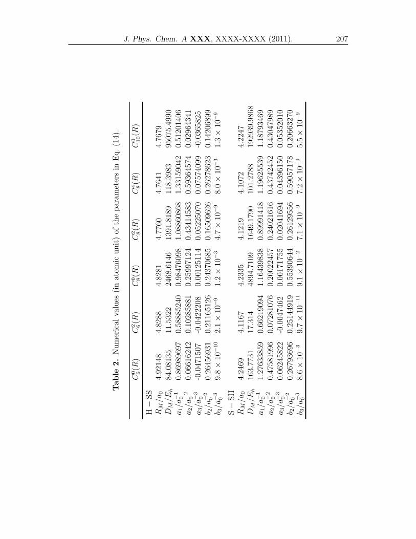
J. Phys. Chem. A XXX, XXXX-XXXX (2011). 207
Table
2.
Nu
mer
ical
valu
es(i
nat
omic
un
it)
ofth
ep
aram
eter
sin
Eq.
(14)
.
C0 6(R
)C
2 6(R
)C
0 8(R
)C
2 8(R
)C
4 8(R
)C
0 10(R
)
H−
SS
RM/a
04.
9214
84.
8288
4.82
814.
7760
4.76
414.
7679
DM/E
h84
.081
3511
.532
224
68.6
146
1391
.818
911
8.39
8395
075.
4990
a1/a
−1
00.
8698
9697
0.58
8852
400.
9847
6098
1.08
8608
681.
3315
9042
0.51
2014
06a
2/a
−2
00.
0661
6242
0.10
2858
810.
2599
7124
0.43
4145
830.
5936
4574
0.02
9643
41a
3/a
−3
0-0
.047
1507
-0.0
4222
080.
0012
5114
0.05
2250
700.
0757
4099
-0.0
3658
25b 2/a
−2
00.
2645
6931
0.21
1651
260.
2437
0685
0.16
5096
260.
2627
8623
0.14
2068
99b 3/a
−3
09.
8×
10−
10
2.1×
10−
91.
2×
10−
34.
7×
10−
98.
0×
10−
31.
3×
10−
9
S−
SH
RM/a
04.
2469
4.11
674.
2335
4.12
194.
1072
4.22
47D
M/E
h16
3.77
3117
.314
4894
.710
916
49.1
790
101.
2788
1929
39.9
868
a1/a
−1
01.
2763
3859
0.66
2190
941.
1643
9838
0.89
9914
181.
1962
5539
1.18
7934
69a
2/a
−2
00.
4758
1996
0.07
2810
760.
2002
2457
0.24
0216
160.
4374
2452
0.43
0479
89a
3/a
−3
00.
0624
5822
-0.0
0474
620.
0017
1755
0.02
0416
940.
0439
6150
0.05
3520
10b 2/a
−2
00.
2679
3696
0.25
1449
190.
5539
0644
0.26
1295
560.
5905
7178
0.20
6632
70b 3/a
−3
08.
6×
10−
39.
7×
10−
11
9.1×
10−
27.
1×
10−
97.
2×
10−
95.
5×
10−
9
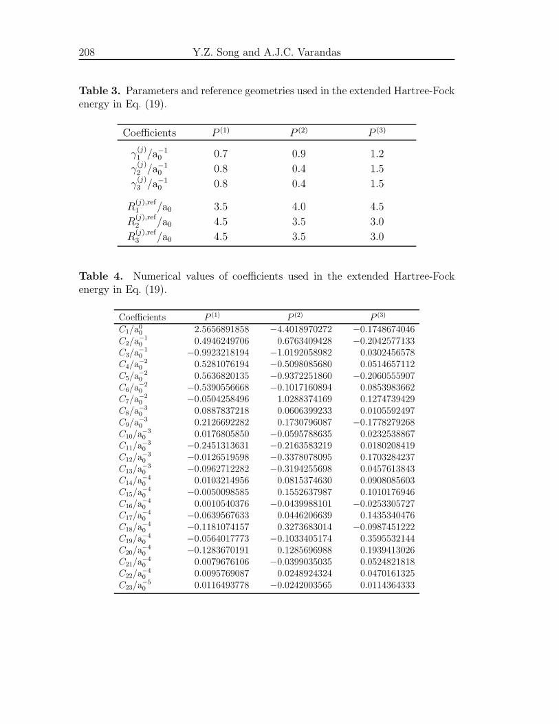
208 Y.Z. Song and A.J.C. Varandas
Table 3. Parameters and reference geometries used in the extended Hartree-Fockenergy in Eq. (19).
Coefficients P (1) P (2) P (3)
γ(j)1 /a−1
0 0.7 0.9 1.2
γ(j)2 /a−1
0 0.8 0.4 1.5
γ(j)3 /a−1
0 0.8 0.4 1.5
R(j),ref1 /a0 3.5 4.0 4.5
R(j),ref2 /a0 4.5 3.5 3.0
R(j),ref3 /a0 4.5 3.5 3.0
Table 4. Numerical values of coefficients used in the extended Hartree-Fockenergy in Eq. (19).
Coefficients P (1) P (2) P (3)
C1/a00 2.5656891858 −4.4018970272 −0.1748674046
C2/a−10 0.4946249706 0.6763409428 −0.2042577133
C3/a−10 −0.9923218194 −1.0192058982 0.0302456578
C4/a−20 0.5281076194 −0.5098085680 0.0514657112
C5/a−20 0.5636820135 −0.9372251860 −0.2060555907
C6/a−20 −0.5390556668 −0.1017160894 0.0853983662
C7/a−20 −0.0504258496 1.0288374169 0.1274739429
C8/a−30 0.0887837218 0.0606399233 0.0105592497
C9/a−30 0.2126692282 0.1730796087 −0.1778279268
C10/a−30 0.0176805850 −0.0595788635 0.0232538867
C11/a−30 −0.2451313631 −0.2163583219 0.0180208419
C12/a−30 −0.0126519598 −0.3378078095 0.1703284237
C13/a−30 −0.0962712282 −0.3194255698 0.0457613843
C14/a−40 0.0103214956 0.0815374630 0.0908085603
C15/a−40 −0.0050098585 0.1552637987 0.1010176946
C16/a−40 0.0010540376 −0.0439988101 −0.0253305727
C17/a−40 −0.0639567633 0.0446206639 0.1435340476
C18/a−40 −0.1181074157 0.3273683014 −0.0987451222
C19/a−40 −0.0564017773 −0.1033405174 0.3595532144
C20/a−40 −0.1283670191 0.1285696988 0.1939413026
C21/a−40 0.0079676106 −0.0399035035 0.0524821818
C22/a−40 0.0095769087 0.0248924324 0.0470161325
C23/a−50 0.0116493778 −0.0242003565 0.0114364333
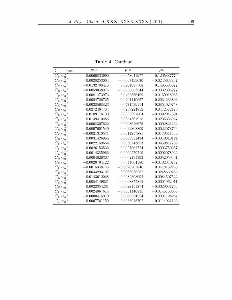
J. Phys. Chem. A XXX, XXXX-XXXX (2011). 209
Table 4. Continue
Coefficients P (1) P (2) P (3)
C24/a−50 0.0060833990 0.0058941977 0.1205887776
C25/a−50 0.0028253004 −0.0067499030 −0.0245638837
C26/a−50 −0.0132788415 0.0264087708 0.1485535677
C27/a−50 −0.0059048074 −0.0088883544 −0.0032306277
C28/a−50 −0.0081473976 −0.0499356499 −0.0150918965
C29/a−50 −0.0054726725 −0.0201440657 0.2034233803
C30/a−50 −0.0038568823 0.0471539114 0.0851029758
C31/a−50 0.0272467784 0.0258224852 0.0412572170
C32/a−50 0.0189176130 0.0083891864 −0.0092047391
C33/a−50 0.0149410485 −0.0354861918 −0.0235335967
C34/a−50 −0.0008307622 0.0008626675 0.0092821262
C35/a−60 −0.0007601549 0.0022808809 −0.0022078766
C36/a−60 −0.0021310571 0.0014257881 0.0179511439
C37/a−60 0.0031426954 0.0068931434 −0.0019840124
C38/a−60 0.0022159664 0.0050743053 0.0459817788
C39/a−60 −0.0026153532 0.0027061724 0.0003750257
C40/a−60 −0.0014385966 −0.0009279219 0.0092078922
C41/a−60 0.0004026307 0.0002131393 −0.0052059461
C42/a−60 −0.0020704122 0.0044064586 −0.0132840747
C43/a−60 −0.0015348145 −0.0020707846 0.0478452266
C44/a−60 −0.0043293107 0.0083085287 0.0248669465
C45/a−60 0.0143612048 0.0082398092 0.0084507522
C46/a−60 0.0054149621 −0.0068855815 −0.0001962011
C47/a−60 0.0022354201 0.0022151274 −0.0329637753
C48/a−60 0.0024867614 −0.0031146835 −0.0146158653
C49/a−60 −0.0000415079 0.0000954224 −0.0001198254
C50/a−60 −0.0007761159 0.0033918702 0.0114931122

Chapter 8
Conclusions and outlook
In the present thesis we reported a series of published results, mainly focused on
the ab initio calculation and modeling of DMBE PESs for the electronic ground-
state H2S and HS2. We have compared the results of the conventional CCSD and
CCSD(T), and the renormalized CR-CCSD(T), CR-CCSD(TQ), CR-CC(2,3),
and CR-CC(2,3)+Q calculations with the MRCI(Q) results for the three impor-
tant cuts of the H2S(1A′) PES. We have found that all renormalized CC methods
reduce the failures of the conventional CCSD and CCSD(T) approaches in the
bond stretching regions of the H2S potential, with the CR-CC(2,3) and CR-
CC(2,3)+Q methods being most effective in this regard.
A global single-sheeted DMBE/CBS PES has been reported for the electronic
ground state of hydrogen sulfide on the basis of a least-squares fit to MRCI(Q)
energies calculated using AVTZ and AVQZ basis sets subsequently extrapolated
to the CBS limit. A global single-sheeted DMBE/SEC PES has also been reported
based on a least-squares fit to MRCI(Q) energies calculated using AVQZ basis sets
subsequently corrected by the DMBE-SEC method. The various topographical
features of the novel DMBE/CBS and DMBE/SEC PESs have been examined in
detail and compared with the other PESs, as well as experiments available in the
literature. The accuracy and consistency of the DMBE-SEC approach has also
been confirmed by comparing the corrected energies with those obtained from
CBS extrapolation. Quasiclassical trajectory studies are also carried out on the
thermal rate constants for S(1D)+H2/D2/HD reactions, which have been shown
to be in good agreement with available experimental and theoretical data, and so
did the vibrational state-resolved ICSs for the S(1D)+H2(ν=0, j=0, 1) reactions.
212 Conclusions and outlook
We have reported a global DMBE/CBS PES for the electronic ground-state
HS2, on the basis of fitting MRCI(Q)/AV(T,Q)dZ energies which are extrapo-
lated to CBS limit. The USTE(T,Q) extrapolation scheme is employed to war-
rant the accuracy of the CBS limit. The DMBE/CBS PES describes all major
topographical features of HS2 PES. Indeed, a comparison of its attributes with
experimental and other accurate theoretical values shows quite a good agreement.
This and the results of preliminary rate constant calculations for S+SH → H+S2
reaction clearly commends the use of the current PES for more detailed adiabatic
dynamics studies of the title reaction.
The PESs reported in the present thesis give a good description of H2S and
HS2 molecular systems. They can be further used to study other reactive pro-
cesses. Finally, they may enable the construction of larger polyatomic DMBE
PES in which H2S and/or HS2 are contained, such as SH3 and H2S2.
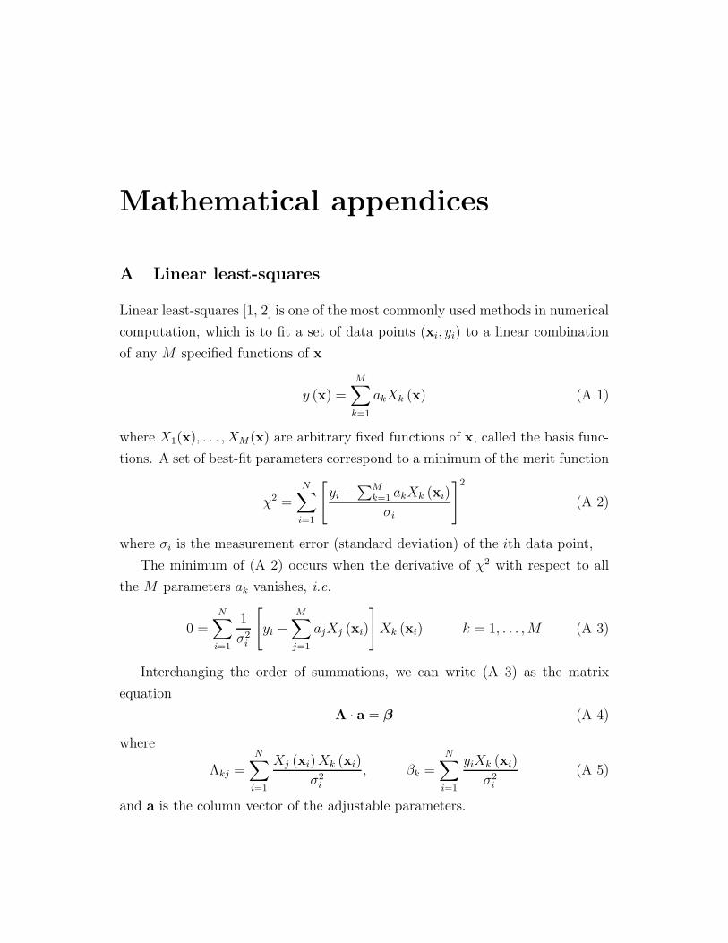
Mathematical appendices
A Linear least-squares
Linear least-squares [1, 2] is one of the most commonly used methods in numerical
computation, which is to fit a set of data points (xi, yi) to a linear combination
of any M specified functions of x
y (x) =
M∑
k=1
akXk (x) (A 1)
where X1(x), . . . , XM(x) are arbitrary fixed functions of x, called the basis func-
tions. A set of best-fit parameters correspond to a minimum of the merit function
χ2 =
N∑
i=1
[yi −
∑Mk=1 akXk (xi)
σi
]2
(A 2)
where σi is the measurement error (standard deviation) of the ith data point,
The minimum of (A 2) occurs when the derivative of χ2 with respect to all
the M parameters ak vanishes, i.e.
0 =
N∑
i=1
1
σ2i
[yi −
M∑
j=1
ajXj (xi)
]Xk (xi) k = 1, . . . ,M (A 3)
Interchanging the order of summations, we can write (A 3) as the matrix
equation
Λ · a = β (A 4)
where
Λkj =N∑
i=1
Xj (xi)Xk (xi)
σ2i
, βk =N∑
i=1
yiXk (xi)
σ2i
(A 5)
and a is the column vector of the adjustable parameters.
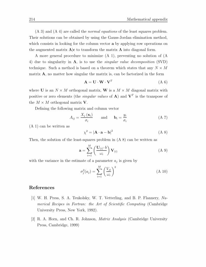
214 Mathematical appendix
(A 3) and (A 4) are called the normal equations of the least squares problem.
Their solutions can be obtained by using the Gauss-Jordan elimination method,
which consists in looking for the column vector a by applying row operations on
the augmented matrix Λ|c to transform the matrix Λ into diagonal form.
A more general procedure to minimize (A 1), preventing no solution of (A
4) due to singularity in Λ, is to use the singular value decomposition (SVD)
technique. Such a method is based on a theorem which states that any N ×M
matrix A, no matter how singular the matrix is, can be factorized in the form
A = U ·W · VT (A 6)
where U is an N ×M orthogonal matrix, W is a M ×M diagonal matrix with
positive or zero elements (the singular values of A) and VT is the transpose of
the M ×M orthogonal matrix V.
Defining the following matrix and column vector
Aij =Xj (xi)
σiand bi =
yi
σi(A 7)
(A 1) can be written as
χ2 = |A · a − b|2 (A 8)
Then, the solution of the least-squares problem in (A 8) can be written as
a =M∑
i=1
(U(i)· bωi
)V(i) (A 9)
with the variance in the estimate of a parameter aj is given by
σ2j (aj) =
M∑
i=1
(Vji
ωi
)2
(A 10)
References
[1] W. H. Press, S. A. Teukolsky, W. T. Vetterling, and B. P. Flannery, Nu-
merical Recipes in Fortran: the Art of Scientific Computing (Cambridge
University Press, New York, 1992).
[2] R. A. Horn, and Ch. R. Johnson, Matrix Analysis (Cambridge University
Press, Cambridge, 1999)
Mathematical appendix 215
B Gamma Function
The Gamma function is defined1 by the integral
Γ(z) ≡∫ ∞
0
tz−1e−tdt (B 1)
When the argument z is an integer, the Gamma function can be written in the
form of a factorial function:
Γ(n+ 1) = n! (B 2)
Gamma function satisfies recurrence relation:
Γ(z + 1) = zΓ(z) (B 3)
The natural logarithm of the Gamma function is implemented in the gammln
function from Numerical recipes.
The Incomplete Gamma Functionis defined by:
P (a, x) ≡ γ(a, x)
Γ(a)≡ 1
Γ(a)
∫ x
0
ta−1e−tdt, (a > 0) (B 4)
It has the limiting values
P (a, 0) = 0 and P (a,∞) = 1 (B 5)
The complement Q(a, x) is:
Q(a, x) ≡ 1 − P (a, x) ≡ 1
Γ(a)
∫ ∞
x
ta−1e−tdt, (a > 0) (B 6)
Functions gammp and gammq from Numerical recipes provides P and Q functions
respectively.
1All definitions and properties from “Numerical Recipes in Fortran ’77”