Unit 3: Computer System Evolution

3.1 Unit Introduction

Welcome to the third unit of Module 1, Computer System Evolution. In

unit 2, you were introduced to computer architecture as comprising the

design of a computer system. In particular, you gained insight into the main

structural components that make up a computer system’s architecture and

into the interactions among these components to achieve the overall

function of a computer, that is, program execution. So far, the previous two

units have introduced computer systems as we know and use them today.

However, as I am sure you are aware, if using computers makes life easier

for us today, we can thank a number of people for their discoveries and

inventions in the computing field.

The field of computing is incredibly fast paced, with dramatic changes

seeming to occur every few years. You only have to look at advances in the

fields of machine learning, automation and artificial intelligence to realise

that the field of computing may look like a very different world in a decade’s

time. Yet it all mostly stems from those simple discoveries made by a

handful of individuals between the late 1930s and the early 1980s.

As I am sure you are aware, a study of history in any field helps us

understand the different changes that have taken place over time and how

these events have influenced the world we live in today. In this unit, you will

be introduced to a number of significant inventions that have taken place

over time in the rapidly changing world of computing. You will also learn

about the direction in which developments in computer architecture are

heading.

3.2 Unit Aims

The aim of this unit is to introduce you to a number of significant

inventions that have taken place over time in the rapidly changing world

of computing.

3.3 Unit Objectives

By the end of this unit, you should be able to:

● Present an overview of the evolution of computer technology from

early human computers to the latest electronic computers.

● Describe the key performance issues that relate to the design of a

computer system.

3.4 Origins of Computation

Electronic computers maybe relatively new, but the need for computation is

not.

The Abacus

The earliest recognised device for computing was the abacus, Figure 3-1, invented in

Mesopotamia around 2700 – 2500 BCE. It’s essentially a hand operated calculator, that

helps add and subtract many numbers. It also stores the current state of the computation,

much like your hard drive does today. Before computers, calculators, or even arithmetic

using paper and pencil, the abacus was the most advanced device for crunching

numbers. Before the abacus, the only methods people had to use for their mathematical

calculations were their fingers and toes, or stones in the dirt.

Figure 3-1: The Abacus

To use the abacus, lay it on a flat surface and set it to zero by making sure no beads are

touching the reckoning bar. To count on the abacus start on the far right side of the

abacus, and slide one earthly bead up to the reckoning bar. For example, in the picture,

the abacus is equal to "283" with nine beads moved towards the reckoning bar.

Figure 3-2: Abacus equal to 283

The third column (100's column) has two beads counted for 200. The second column

(10's column) has a Heavenly bead counted for 50, and three Earthly beads counted for

30 giving it a total of 80. Finally, the first column (1's column) has three beads counted.

Adding all columns together (200 + 80 + 3) gives you the total of 283.

Over the next thousands of years, humans developed all sorts of clever computing

devices, each one of these devices making something that was previously laborious to

calculate much faster, easier, and often more accurate. Two prominent examples are

Napier’s Bones and the Slide Rule.

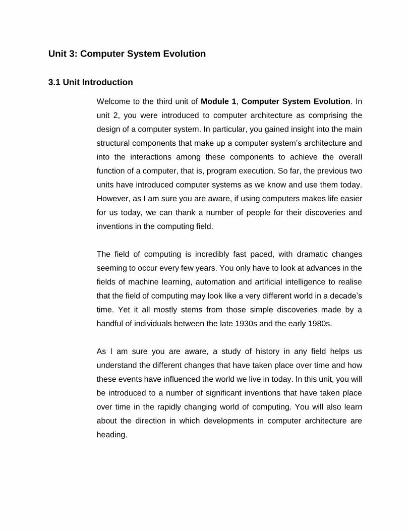
Napier’s Bones - 1614

John Napier invented this aid that reduced division to a process of subtraction and

multiplication to a process of addition.

Figure 3-3: The Slide Rule

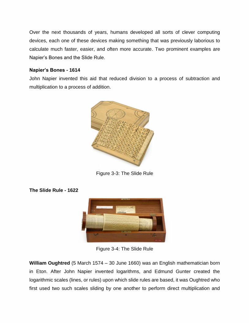
The Slide Rule - 1622

Figure 3-4: The Slide Rule

William Oughtred (5 March 1574 – 30 June 1660) was an English mathematician born

in Eton. After John Napier invented logarithms, and Edmund Gunter created the

logarithmic scales (lines, or rules) upon which slide rules are based, it was Oughtred who

first used two such scales sliding by one another to perform direct multiplication and

division; and he is credited as the inventor of the slide rule in 1622. Oughtred also

introduced the "×" symbol for multiplication as well as the abbreviations "sin" and "cos"

for the sine and cosine functions.

3.5 Mechanical Computation

A mechanical computer is one that is built from mechanical components such

as levers and gears.

These devices were unlike the previous simple inventions. The most common types of

mechanical computers are adding machines and mechanical counters, which use the

turning of gears to increment numbers. Some notable examples include:

Wilhelm Schickard’s Calculator – Around 1623

Figure 3-5: Schickard’s Calculator

Wilhelm Schickard, a German astronomer and mathematician, is credited for inventing

the world’s first mechanical calculator. The machine could add and subtract six-digit

numbers, and indicated an overflow of this capacity by ringing a bell; to add more complex

calculations, a set of Napier's bones were mounted on it. Unlike other devices of its time

which relied on a human operator to change different portions, his device was a state

machine. In different situations, gears would be placed and interact with each other

mechanically. It was also the first calculator that was active, meaning that each number

inputted modified others.

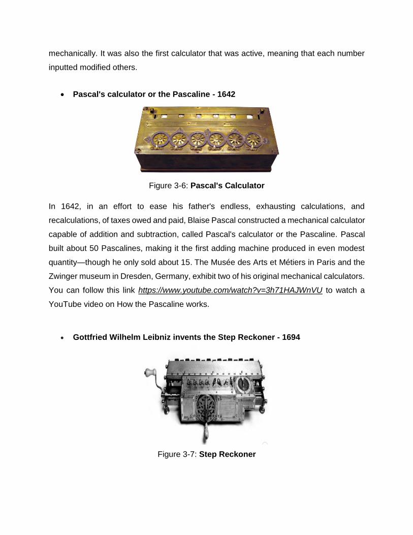
Pascal's calculator or the Pascaline - 1642

Figure 3-6: Pascal's Calculator

In 1642, in an effort to ease his father's endless, exhausting calculations, and

recalculations, of taxes owed and paid, Blaise Pascal constructed a mechanical calculator

capable of addition and subtraction, called Pascal's calculator or the Pascaline. Pascal

built about 50 Pascalines, making it the first adding machine produced in even modest

quantity—though he only sold about 15. The Musée des Arts et Métiers in Paris and the

Zwinger museum in Dresden, Germany, exhibit two of his original mechanical calculators.

You can follow this link https://www.youtube.com/watch?v=3h71HAJWnVU to watch a

YouTube video on How the Pascaline works.

Gottfried Wilhelm Leibniz invents the Step Reckoner - 1694

Figure 3-7: Step Reckoner

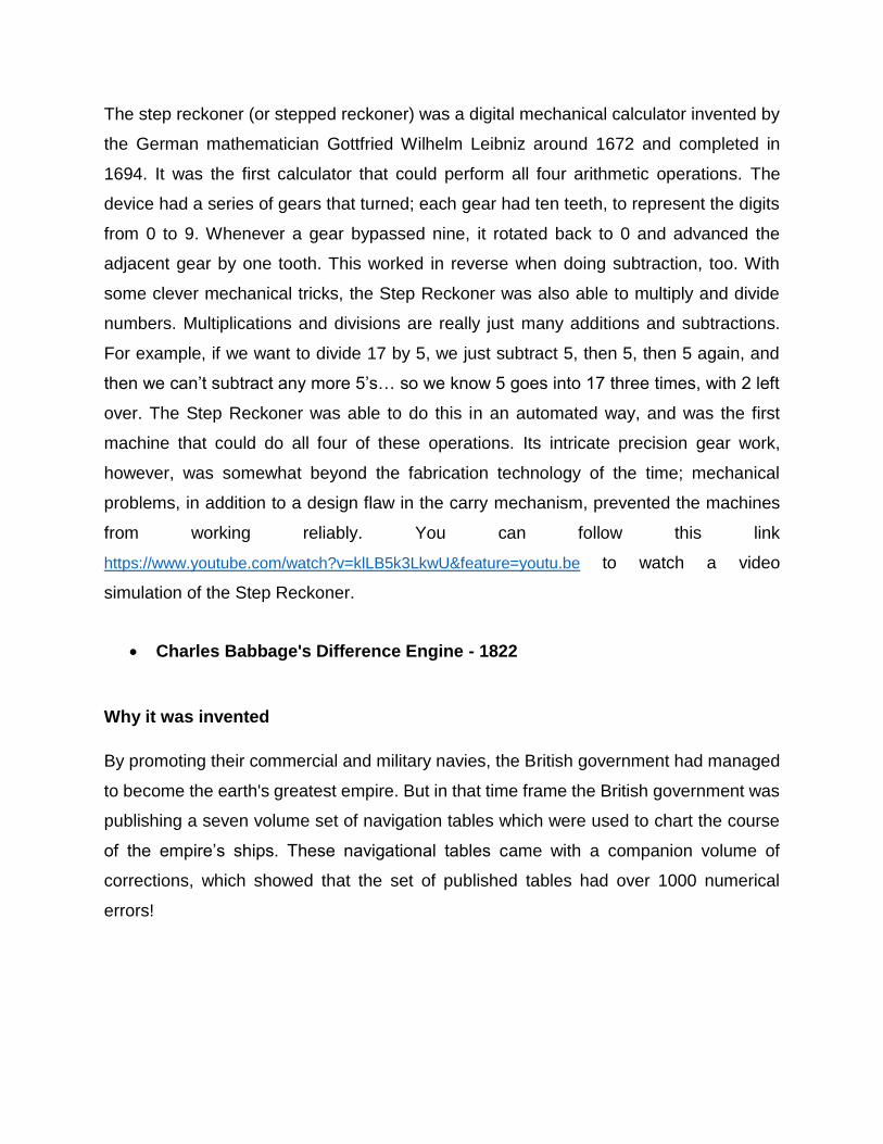
The step reckoner (or stepped reckoner) was a digital mechanical calculator invented by

the German mathematician Gottfried Wilhelm Leibniz around 1672 and completed in

1694. It was the first calculator that could perform all four arithmetic operations. The

device had a series of gears that turned; each gear had ten teeth, to represent the digits

from 0 to 9. Whenever a gear bypassed nine, it rotated back to 0 and advanced the

adjacent gear by one tooth. This worked in reverse when doing subtraction, too. With

some clever mechanical tricks, the Step Reckoner was also able to multiply and divide

numbers. Multiplications and divisions are really just many additions and subtractions.

For example, if we want to divide 17 by 5, we just subtract 5, then 5, then 5 again, and

then we can’t subtract any more 5’s… so we know 5 goes into 17 three times, with 2 left

over. The Step Reckoner was able to do this in an automated way, and was the first

machine that could do all four of these operations. Its intricate precision gear work,

however, was somewhat beyond the fabrication technology of the time; mechanical

problems, in addition to a design flaw in the carry mechanism, prevented the machines

from working reliably. You can follow this link

https://www.youtube.com/watch?v=klLB5k3LkwU&feature=youtu.be to watch a video

simulation of the Step Reckoner.

Charles Babbage's Difference Engine - 1822

Why it was invented

By promoting their commercial and military navies, the British government had managed

to become the earth's greatest empire. But in that time frame the British government was

publishing a seven volume set of navigation tables which were used to chart the course

of the empire’s ships. These navigational tables came with a companion volume of

corrections, which showed that the set of published tables had over 1000 numerical

errors!

Figure 3.8: A small section of the type of mechanism employed in Babbage's

Difference Engine [photo © 2002 IEEE]

The Proposed Mechanical Computer Solution

Charles Babbage proposed a new mechanical device called the Difference Engine, a

much more complex machine that could approximate polynomials. Polynomials describe

the relationship between several variables - like range and air pressure, Polynomials

could also be used to approximate logarithmic and trigonometric functions, which are a

real hassle to calculate by hand. Babbage started construction in 1823, and over the next

two decades, tried to fabricate and assemble the 25,000 components, collectively

weighing around 15 tons. Unfortunately, the project was ultimately abandoned. But, in

1991, historians finished constructing a Difference Engine based on Babbage's drawings

and writings - and it worked! Check it out at this link, https://youtu.be/be1EM3gQkAY

(Difference Engine No. 2, built faithfully to the original drawings, consists of 8,000 parts,

weighs five tons, and measures 11 feet long.

Charles Babbage's Analytical Engine

During construction of the Difference Engine, Babbage imagined an even more complex

machine - the Analytical Engine. Unlike the Difference Engine, Step Reckoner and all

other computational devices before it - the Analytical Engine was a “general purpose

computer”. It could be used for many things, not just one particular computation; it could

be given data and run operations in sequence; it had memory and even a primitive printer.

Like the Difference Engine, it was ahead of its time, and was never fully constructed.

However, the idea of an “automatic computer” – one that could guide itself through a

series of operations automatically, was a huge deal, and would foreshadow computer

programs.

English mathematician Ada Lovelace wrote hypothetical programs for the Analytical

Engine. For her work, Ada is often considered the world’s first programmer. The Analytical

Engine would inspire, arguably, the first generation of computer scientists, who

incorporated many of Babbage’s ideas in their machines. This is why Babbage is often

considered the "father of computing".

Over many years, a number of inventors proposed a variety of mechanical computers.

Unfortunately, even with mechanical calculators, most real world problems required many

steps of computation before an answer was determined. It could take hours or days to

generate a single result. Also, these hand-crafted machines were expensive, and not

accessible to most of the population.

Activity 3.1: Using the Internet, search for information on the Hollerith

desk.

1. When was it invented, and by whom?

2. What computational challenge did the inventor address?

3. What was the proposed solution? Did it work?

1.5 Electromechanical Computation

The second mechanisms invented for the purpose of performing calculations were

electromechanical computers.

An electromechanical computer is one that was built from both electronic

components such as relays (i.e., electrically-controlled mechanical switches) and

mechanical components such as levers and gears.

These devices were unlike the previous purely mechanical inventions. One notable

example is the Harvard Mark I:

Howard Aiken’s Mark I - 1944

Figure 3-9: Harvard Mark I

In 1944 IBM introduced the automatic sequence controlled calculator (ASCC), the largest

electromechanical calculator built. It was a general-purpose electromechanical computer

that was used in the war effort during the last part of World War II. The original concept

for this giant calculator was presented to IBM by Dr. Howard Aiken in November of 1937.

The ASCC was developed and built by IBM then shipped to Harvard in February 1944

where it became known as the Harvard mark 1 by University staff and others. The mark

1 was the first operating machine that could execute long computations automatically.

The Mark I was:

51 feet long,

used 500 miles of wire

had over 3 million connections

3500 relays and thousands of counters and switches

It read its instructions from a 24 channel punched paper tape

Check it out at this link, https://www.youtube.com/watch?v=bN7AdQmd8So&t=29s

One limitation of electromechanical devices is wear and tear. Anything mechanical that

moves will wear over time. Some things break entirely, and other things start getting

sticky, slow, and just plain unreliable. And as the number of relays increases, the

probability of a failure increases too. The Harvard Mark I had roughly 3500 relays.

These huge, dark, and warm machines also attracted insects. In September 1947,

operators on version two, the Harvard Mark II pulled a dead moth from a malfunctioning

relay. From then on, when anything went wrong with a computer, they said it had bugs

in it. And that’s where the term computer bug comes from. In 1959 after 15 years of

service the mark 1 was officially taken offline. Portions of it remain at Harvard University

today.

Other notable examples of electromechanical computers include the Mark

II, and Zuse Computers (Z2, Z3). You can look up information on these examples to widen

your knowledge on the era of electromechanical computers.

It was clear that a faster, more reliable alternative to electromechanical relays was

needed if computing was going to advance further, and fortunately that alternative already

existed! In 1904, English physicist John Ambrose Fleming developed a new electrical

component called a thermionic valve, which housed two electrodes inside an airtight glass

bulb - this was the first vacuum tube. The use of vacuum tubes in computation devices

ushered in the era of electronic computation.

3.6 Electronic Computation

An electronic computer is one that is built from electronic components such as

vacuum tubes, transistors and integrated circuits, rather than mechanical components

such as levers and gears.

The inventions of electronic computers can be organised according to the different types

of electronic technology they used. These electronic technologies are vacuum tubes,

transistors and integrated circuits. Let us examine how each type of these electronic

technologies changed the history of computing.

3.6.1 The First Generation: Vacuum Tubes

The first generation of electronic computers used vacuum tubes (see Figure 1.2).

A vacuum tube is an electronic device that controls the flow of electrons (primary

carriers of electricity) in a vacuum (a space from which almost all air or gas has been

evacuated).

Please note: the focus of this unit are the technological advances in the history of

computers. As such, only a brief overview of the electronic devices is provided for

introductory purposes.

Figure 3-10: A Basic Vacuum Tube [photo © Collectors Weekly]

How a Vacuum Tube Works

Current passing through the filament (or cathode) heats it up so that it gives off electrons.

These, being negatively charged, are attracted to the positive plate (or anode). A grid of

wires between the filament and the plate is negative, which repels the electrons and

hence controls the current to the plate. When used as on/off switches, vacuum tubes

allowed the first electronic computers to perform digital computations. That is, to

generate, store, and process data (any set of values) in terms of two states: positive and

non-positive. Other than electronic computers, some other applications of vacuum tubes

you might be familiar with are switches, audio amplifiers and television display screens.

Let us now examine two notable electronic computer inventions that used vacuum tubes:

the Colossus and ENIAC (Electronic Numerical Integrator and Computer).

Colossus (Tommy Flowers) - 1943

The first large-scale use of vacuum tubes for computing was the Colossus designed by

engineer Tommy Flowers and completed in December of 1943. The Colossus was

installed at Bletchley Park, in the UK, and helped to decrypt Nazi communications. The

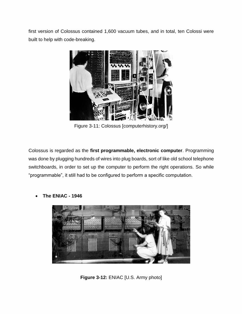
first version of Colossus contained 1,600 vacuum tubes, and in total, ten Colossi were

built to help with code-breaking.

Figure 3-11: Colossus [computerhistory.org/]

Colossus is regarded as the first programmable, electronic computer. Programming

was done by plugging hundreds of wires into plug boards, sort of like old school telephone

switchboards, in order to set up the computer to perform the right operations. So while

“programmable”, it still had to be configured to perform a specific computation.

The ENIAC - 1946

Figure 3-12: ENIAC [U.S. Army photo]

In computing history, the ENIAC is believed to be the world’s first truly general purpose,

programmable, electronic computer. It was designed and constructed at the University

of Pennsylvania in the United States (U.S.) between 1943 and 1946 by two professors,

John Mauchly, a professor of electrical engineering, and John Eckert, one of his graduate

students. ENIAC was enormous, weighing 30 tons (over 27,000 kg!), occupying 1500

square feet of floor space, and containing more than 18,000 vacuum tubes. When

operating, it consumed 140 kilowatts of power.

ENIAC could perform 5000 ten-digit additions or subtractions per second, many, many

times faster than any machine that came before it. To give you an example, the very first

problem run on ENIAC required only 20 seconds and was checked against an answer

obtained after forty hours of work with a mechanical calculator.

The ENIAC was completed in 1946, too late to be used in the war effort. So instead, its

first task was to perform a series of complex calculations that were used to help determine

the possibility of building a hydrogen bomb (a very powerful weapon capable of wiping

out an entire city!). The use of the ENIAC for a purpose other than that for which it was

built demonstrated its general- purpose nature. The ENIAC continued to operate under

BRL management until 1955, when it was disassembled.

By the 1950’s, even vacuum-tube-based computing was reaching its limits. The use of

vacuum tube technology presented two major disadvantages,

1. vacuum tubes require a large amount of power supply, and

2. high voltages present an electric shock hazard.

For instance, vacuum tube failures were so common on the ENIAC that it was generally

only operational for about half a day at a time before breaking down. To reduce cost and

size, as well as improve reliability and speed, a radical new electronic switch would be

needed. In 1947, Bell Laboratory scientists John Bardeen, Walter Brattain, and William

Shockley invented the transistor, and with it, a whole new era of computing was born!

3.6.2 The Second Generation: Transistors

A transistor is a semiconductor device used to amplify or switch electronic signals

and electrical power.

Figure 3-13: Transistors [photo © Bell Laboratories 1947]

The physics behind transistors is complex, relying on quantum mechanics. This unit

presents the basics. A transistor, like a relay or vacuum tube, is a switch that can be

opened or closed by applying electrical power via a control wire. Typically, transistors

have two electrodes separated by a material that sometimes can conduct electricity, and

other times resist it – a semiconductor. In this case, the control wire attaches to a “gate”

electrode. By changing the electrical charge of the gate, the conductivity of the

semiconducting material can be manipulated, allowing current to flow or be stopped.

The first transistor at Bell Labs could switch between on and off states 10,000 times per

second. The specific improvements or advancements of transistor based computers over

vacuum tube computing can be summarised as follows.

● Unlike vacuum tubes, which require wires, metal plates, a glass capsule, and a

vacuum, the transistor is a solid-state device, made from material called silicon.

● The transistor is also smaller, cheaper, and dissipates less heat than a vacuum

tube. But it can still be used in the same way as a vacuum tube to construct

computers. These characteristics enabled transistors to bring in greater

processing performance, larger memory capacity, and smaller size machines than

the vacuum tube computers.

● Transistor based computers saw the introduction of more complex 65, and control

units. `

The IBM 608 – 1957

Figure 3-14: Photo: From the IBM 608 Calculator Manual of Operation, Form 22-6666-1 (1957). http://www.columbia.edu/cu/computinghistory/608.html

The IBM 608, released in 1957 was the first fully transistor-powered, commercially

available computer. It contained 3000 transistors and could perform 4,500 additions, or

roughly 80 multiplications or divisions, every second. IBM soon transitioned all of its

computing products to transistors, bringing transistor-based computers into offices, and

eventually, homes.

The Challenge of Using Transistors

A single, self-contained transistor is called a discrete component. Throughout the 1950s

and early 1960s, electronic equipment was composed largely of discrete components

such as transistors, resistors, capacitors, and so on. Discrete components were

manufactured separately, packaged in their own containers, and soldered or wired

together onto masonite-like (a type of hardboard) circuit boards, which were then installed

in computers, oscilloscopes, and other electronic equipment. Whenever an electronic

device called for a transistor, a little tube of metal containing a pinhead-sized piece of

silicon had to be soldered to a circuit board. The entire manufacturing process, from

transistor to circuit board, was expensive and cumbersome.

It is no wonder that these facts of life were beginning to create problems in the computer

industry. Early second-generation computers contained about 10,000 transistors. This

figure grew to the hundreds of thousands, making the manufacture of newer, more

powerful machines increasingly difficult. In 1958 came the achievement that

revolutionised electronics and started the era of microelectronics (small electronics): the

invention of the integrated circuit. It is the integrated circuit that defines the third

generation of computers.

3.6.3 The Third Generation: Integrated Circuits

The basic functions of a digital computer, as discussed in the previous unit, are storage,

movement, processing, and control. To perform these functions, only two fundamental

types of components are required: gates and memory cells.

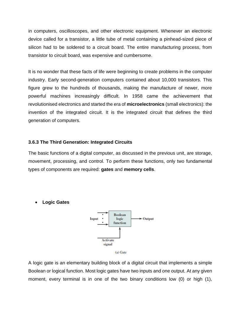
Logic Gates

A logic gate is an elementary building block of a digital circuit that implements a simple

Boolean or logical function. Most logic gates have two inputs and one output. At any given

moment, every terminal is in one of the two binary conditions low (0) or high (1),

represented by different voltage levels. The logic state of a terminal can, and generally

does, change often, as the circuit processes data. In most logic gates, the low state is

approximately zero volts (0 V), while the high state is approximately five volts positive (+5

V).

There are seven basic logic gates: AND, OR, XOR, NOT, NAND, NOR, and XNOR.

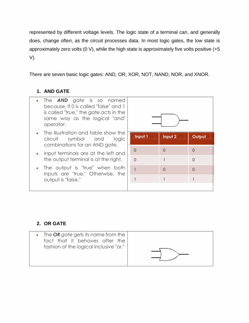
1. AND GATE

The AND gate is so named

because, if 0 is called "false" and 1

is called "true," the gate acts in the

same way as the logical "and"

operator.

The illustration and table show the

circuit symbol and logic

combinations for an AND gate.

Input terminals are at the left and

the output terminal is at the right.

The output is "true" when both

inputs are "true." Otherwise, the

output is "false."

Input 1 Input 2 Output

0 0 0

0 1 0

1 0 0

1 1 1

2. OR GATE

The OR gate gets its name from the

fact that it behaves after the

fashion of the logical inclusive "or."

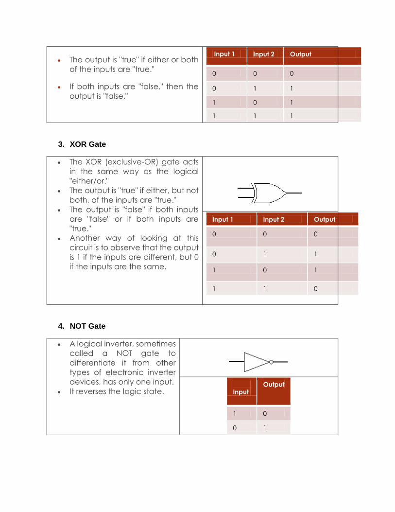
The output is "true" if either or both

of the inputs are "true."

If both inputs are "false," then the

output is "false."

Input 1 Input 2 Output

0 0 0

0 1 1

1 0 1

1 1 1

3. XOR Gate

The XOR (exclusive-OR) gate acts

in the same way as the logical

"either/or."

The output is "true" if either, but not

both, of the inputs are "true."

The output is "false" if both inputs

are "false" or if both inputs are

"true."

Another way of looking at this

circuit is to observe that the output

is 1 if the inputs are different, but 0

if the inputs are the same.

Input 1 Input 2 Output

0 0 0

0 1 1

1 0 1

1 1 0

4. NOT Gate

A logical inverter, sometimes

called a NOT gate to

differentiate it from other

types of electronic inverter

devices, has only one input.

It reverses the logic state.

Input Output

1 0

0 1

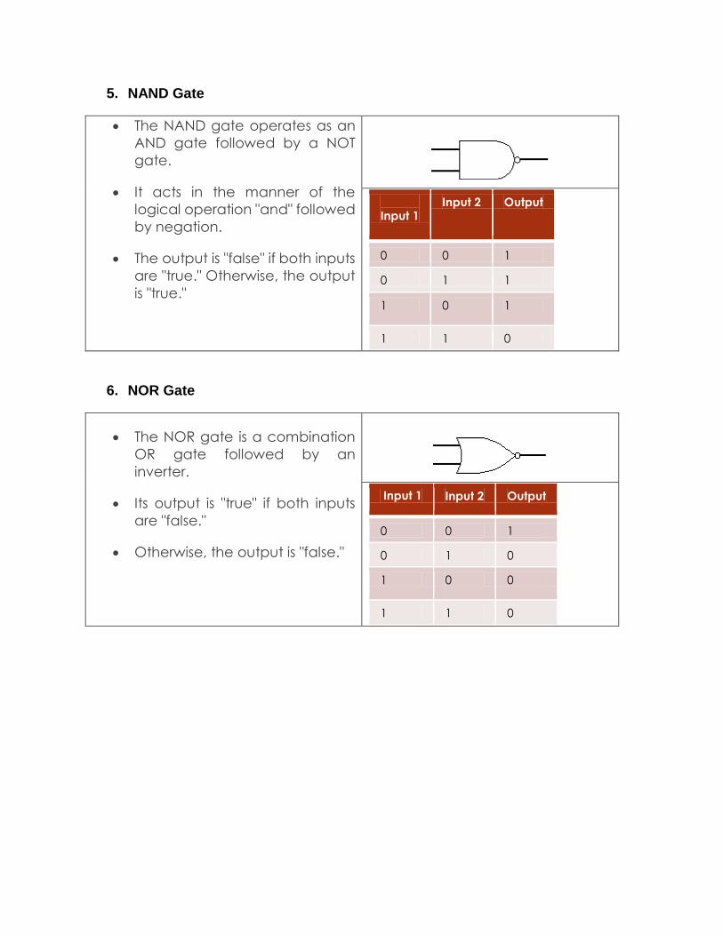
5. NAND Gate

The NAND gate operates as an

AND gate followed by a NOT

gate.

It acts in the manner of the

logical operation "and" followed

by negation.

The output is "false" if both inputs

are "true." Otherwise, the output

is "true."

Input 1

Input 2 Output

0 0 1

0 1 1

1 0 1

1 1 0

6. NOR Gate

The NOR gate is a combination

OR gate followed by an

inverter.

Its output is "true" if both inputs

are "false."

Otherwise, the output is "false."

Input 1 Input 2 Output

0 0 1

0 1 0

1 0 0

1 1 0

7. XNOR GATE

The XNOR (exclusive-NOR)

gate is a combination XOR gate

followed by an inverter.

Its output is "true" if the inputs are

the same, and "false" if the inputs

are different.

Input 1

Input 2 Output

0 0 1

0 1 0

1 0 0

1 1 1

Memory Cells

The memory cell is a device that can store one bit of data. It exhibits two stable (or semi-

stable) states, which can be used to represent binary 1 and 0. It is capable of being written

into (at least once), to set the state. It is also capable of being read to sense the state.

Memory Cell Operation

It has three functional terminals capable of carrying an electrical signal;

Select - selects a memory cell for a read or write operation.

Control - indicates read or write

Data in –

for writing, the other terminal provides an electrical signal that sets the state of the cell to 1 or 0.

for reading, that terminal is used for output of the cell’s state.

To summarise:

Logic Gate

A gate will have one or two data inputs plus a control signal input that

activates the gate.

When the control signal is ON, the gate performs its function on the data

inputs and produces a data output.

Memory Cell

A memory cell will store the bit that is on its input lead when the WRITE

control signal is ON and will place the bit that is in the cell on its output lead

when the READ control signal is ON.

Basic Elements of a Digital Computer

By interconnecting large numbers of logic gates and memory cells, a computer can be

constructed as follows:

Data storage: Provided by memory cells.

Data processing: Provided by gates.

Data movement: The paths among components are used to move data through

gates to memory.

Control: The paths among components can carry control signals.

In this way, a computer can be seen as consisting of gates, memory cells, and

interconnections among these elements. The gates and memory cells are, in turn,

constructed of simple digital electronic components, which are then packaged into

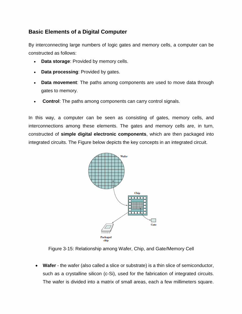
integrated circuits. The Figure below depicts the key concepts in an integrated circuit.

Figure 3-15: Relationship among Wafer, Chip, and Gate/Memory Cell

Wafer - the wafer (also called a slice or substrate) is a thin slice of semiconductor,

such as a crystalline silicon (c-Si), used for the fabrication of integrated circuits.

The wafer is divided into a matrix of small areas, each a few millimeters square.

The identical circuit pattern is fabricated in each area, and the wafer is then broken

up into chips.

Chip (Integrated Circuit) - Each chip consists of many gates and/or memory

cells plus a number of input and output attachment points. This chip is then

packaged in housing that protects it and provides pins for attachment to devices

beyond the chip. A number of these packages can then be interconnected on a

printed circuit board to produce larger and more complex circuits. Follow this link

[https://www.computerhistory.org/revolution/digital-logic/12/288/2220] to watch a

video on integrated circuit design and manufacturing from sand to silicon.

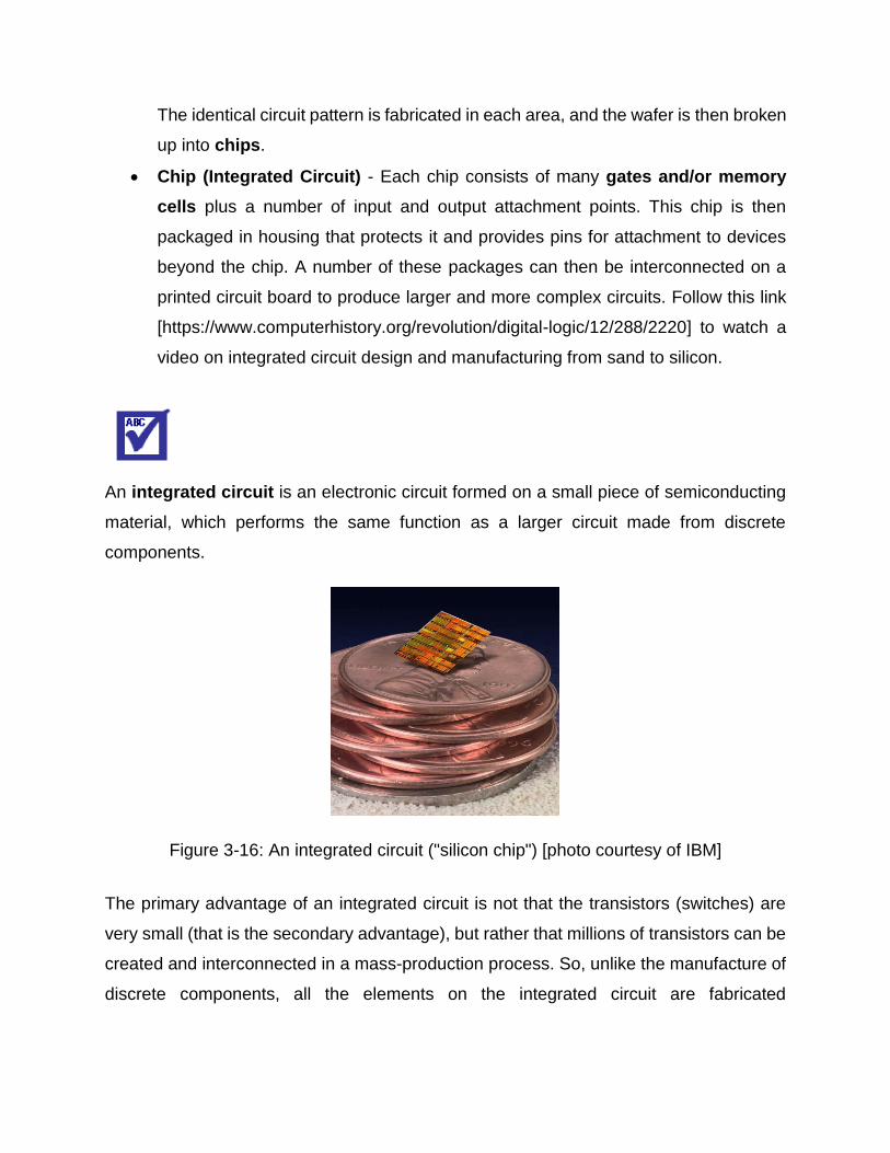
An integrated circuit is an electronic circuit formed on a small piece of semiconducting

material, which performs the same function as a larger circuit made from discrete

components.

Figure 3-16: An integrated circuit ("silicon chip") [photo courtesy of IBM]

The primary advantage of an integrated circuit is not that the transistors (switches) are

very small (that is the secondary advantage), but rather that millions of transistors can be

created and interconnected in a mass-production process. So, unlike the manufacture of

discrete components, all the elements on the integrated circuit are fabricated

simultaneously via a small number of optical masks that define the geometry of each

layer. This speeds up the process of fabricating the computer, and hence reduces its cost.

The two most important members of the third generation, both of which were introduced

at the beginning of that era are the IBM System/360 and the DEC PDP-8 (you may look

up further information on these computers for your own self learning).

3.6.4 Later Generations

At this stage you may be wondering about how many more computer generations there

are. Well actually, beyond the third generation there is less general agreement on defining

generations of computers. As you can see from Table 1.1 below, experts suggest that

there have been a number of later generations, based on advances in integrated circuit

technology.

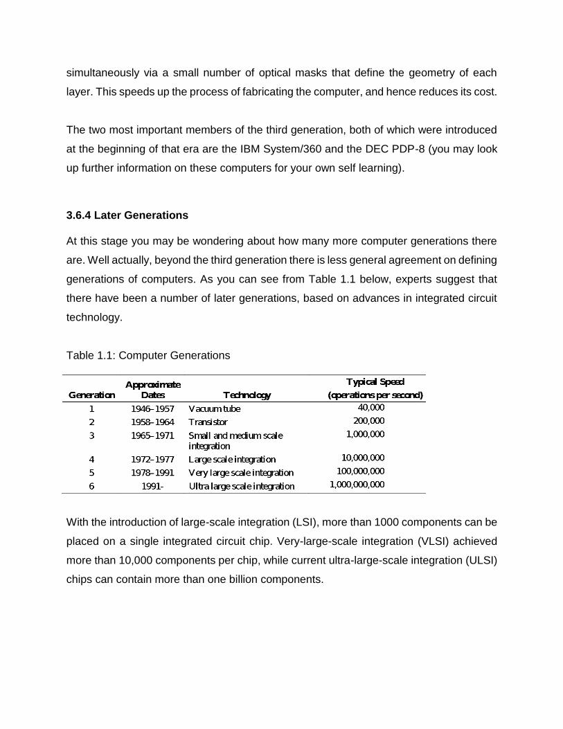
Table 1.1: Computer Generations

With the introduction of large-scale integration (LSI), more than 1000 components can be

placed on a single integrated circuit chip. Very-large-scale integration (VLSI) achieved

more than 10,000 components per chip, while current ultra-large-scale integration (ULSI)

chips can contain more than one billion components.

3.7 The Origins of Computer Architecture

The previous unit introduced computer architecture as comprising the design of a

computer system. However, so far in this unit, our study of the evolution of

computing has provided insight into the development of hardware components

across the history of computing, saying nothing about the origins of computing

architecture. This section fills that gap.

3.7.1 The Stored Programme Concept

The origins of the modern day computer architecture can be traced to the extremely

tedious task of entering and altering programs faced by the ENIAC operators. The ENIAC

designers, most notably the mathematician John von Neumann, who was a consultant

on the ENIAC project proposed a solution to this challenge called the Stored Programme

Concept.

THE VON NEUMANN Architecture

Suppose the sequence of computation steps (programs) could be represented in a form

suitable for storing in memory alongside the values to be operated on (the data). Then, if

information about computation steps was stored in memory, a computer could get its

instructions by reading them from memory. In this way, a program could be set or altered

by setting the values of a portion of memory, rather than a physical modification of all the

patch cords and switches. This idea is known as the stored-program concept.

In 1946, Von Neumann and his colleagues began the design of a new stored-program

computer, referred to as the IAS computer, at the Princeton Institute for Advanced

Studies (IAS). The IAS computer, although not completed until 1952, is the prototype or

template of all subsequent general-purpose computers. Figure 3.17 shows the

general structure of the IAS computer.

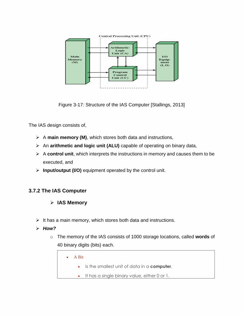
Figure 3-17: Structure of the IAS Computer [Stallings, 2013]

The IAS design consists of,

A main memory (M), which stores both data and instructions,

An arithmetic and logic unit (ALU) capable of operating on binary data,

A control unit, which interprets the instructions in memory and causes them to be

executed, and

Input/output (I/O) equipment operated by the control unit.

3.7.2 The IAS Computer

IAS Memory

It has a main memory, which stores both data and instructions.

How?

o The memory of the IAS consists of 1000 storage locations, called words of

40 binary digits (bits) each.

A Bit

Is the smallest unit of data in a computer.

It has a single binary value, either 0 or 1.

Although computers usually provide instructions that can

test and manipulate bits, they generally are designed to

store data and execute instructions in bit multiples called

bytes (8 bits = 1 byte).

There is no universal definition of the term word. In general, a word

is an ordered set of bytes or bits that is the normal unit in which

information may be stored, transmitted, or operated on within a

given computer.

Typically, if a processor has a fixed-length instruction set, then the

instruction length equals the word length.

o Both data and instructions in the IAS are stored in the memory locations.

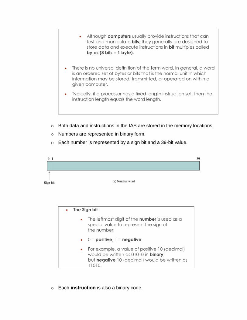
o Numbers are represented in binary form.

o Each number is represented by a sign bit and a 39-bit value.

The Sign bit

The leftmost digit of the number is used as a

special value to represent the sign of

the number:

0 = positive, 1 = negative.

For example, a value of positive 10 (decimal)

would be written as 01010 in binary,

but negative 10 (decimal) would be written as

11010.

o Each instruction is also a binary code.

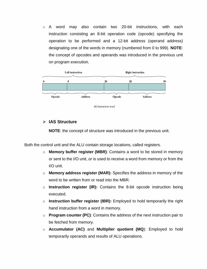
o A word may also contain two 20-bit instructions, with each

instruction consisting an 8-bit operation code (opcode) specifying the

operation to be performed and a 12-bit address (operand address)

designating one of the words in memory (numbered from 0 to 999). NOTE:

the concept of opcodes and operands was introduced in the previous unit

on program execution.

IAS Structure

NOTE: the concept of structure was introduced in the previous unit.

Both the control unit and the ALU contain storage locations, called registers.

o Memory buffer register (MBR): Contains a word to be stored in memory

or sent to the I/O unit, or is used to receive a word from memory or from the

I/O unit.

o Memory address register (MAR): Specifies the address in memory of the

word to be written from or read into the MBR.

o Instruction register (IR): Contains the 8-bit opcode instruction being

executed.

o Instruction buffer register (IBR): Employed to hold temporarily the right

hand instruction from a word in memory.

o Program counter (PC): Contains the address of the next instruction pair to

be fetched from memory.

o Accumulator (AC) and Multiplier quotient (MQ): Employed to hold

temporarily operands and results of ALU operations.

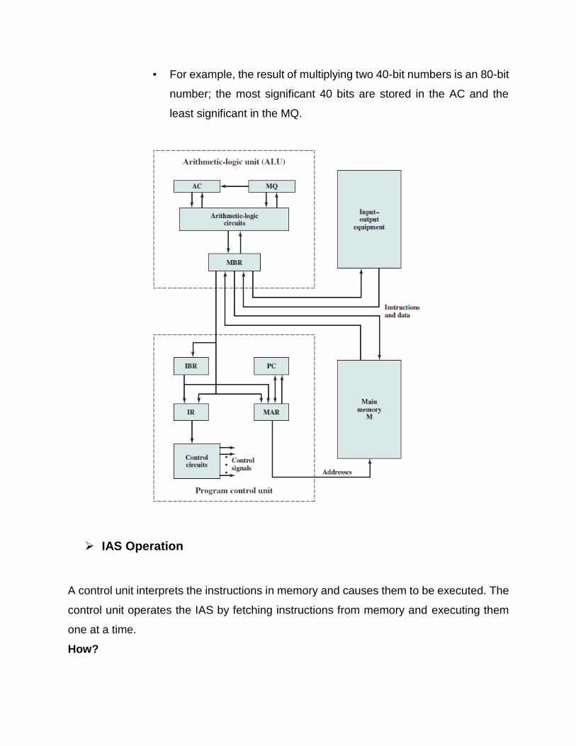
▪ For example, the result of multiplying two 40-bit numbers is an 80-bit

number; the most significant 40 bits are stored in the AC and the

least significant in the MQ.

IAS Operation

A control unit interprets the instructions in memory and causes them to be executed. The

control unit operates the IAS by fetching instructions from memory and executing them

one at a time.

How?

The IAS operates by repetitively performing an instruction cycle. Each instruction cycle

consists of two sub-cycles: Fetch and Execute.

Fetch Cycle

o The opcode of the next instruction is loaded into the IR and the address

portion is loaded into the MAR.

o This instruction may be taken from the IBR, or it can be obtained from

memory by loading a word into the MBR, and then down to the IBR, IR, and

MAR.

o Once the opcode is in the IR, the execute cycle is performed.

o Control circuitry interprets the opcode and executes the instruction by

sending out the appropriate control signals to cause data to be moved or an

operation to be performed by the ALU.

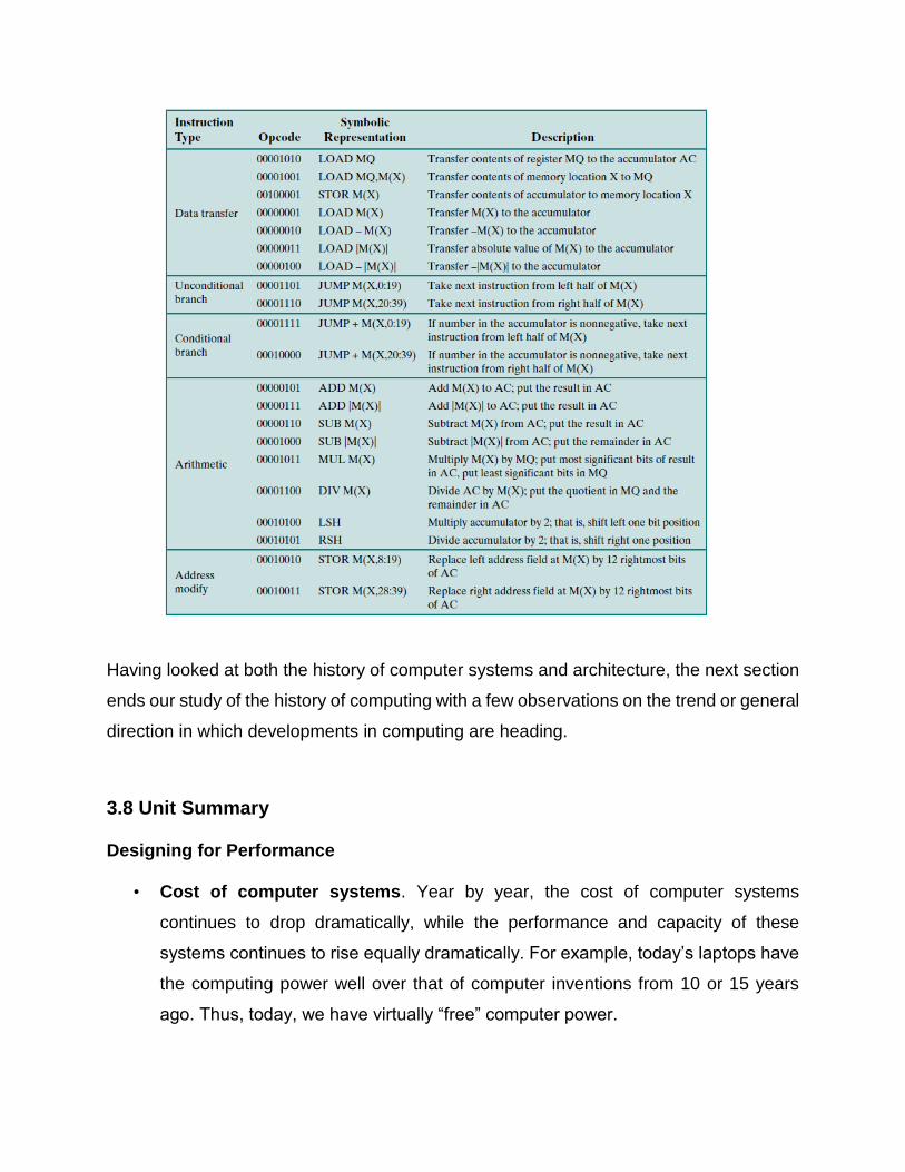
Execute Cycle

The IAS computer had a total of 21 instructions.

o Data Transfer Instructions: Move data between memory and ALU

registers or between two ALU registers.

o Unconditional branch: Normally, the control unit executes instructions in

sequence from memory. This sequence can be changed by a branch

instruction, which facilitates repetitive operations.

o Conditional branch: The branch can be made dependent on a condition,

thus allowing decision points.

o Arithmetic: Operations performed by the ALU.

o Address modify: Permits addresses to be computed in the ALU and

then inserted into instructions stored in memory. This allows a program

considerable addressing flexibility.

Having looked at both the history of computer systems and architecture, the next section

ends our study of the history of computing with a few observations on the trend or general

direction in which developments in computing are heading.

3.8 Unit Summary

Designing for Performance

• Cost of computer systems. Year by year, the cost of computer systems

continues to drop dramatically, while the performance and capacity of these

systems continues to rise equally dramatically. For example, today’s laptops have

the computing power well over that of computer inventions from 10 or 15 years

ago. Thus, today, we have virtually “free” computer power.

• Design of computer systems. What is fascinating about the relationship between

the cost and performance of computers is that, on the one hand, the basic building

blocks for today’s computer miracles are virtually the same as those of the IAS

(Von Neumann) computer from over 50 years ago, while on the other hand, the

techniques for squeezing the last bit of performance out of the materials at hand

have become increasingly sophisticated. Indeed, this observation serves as a

guiding principle for the presentation in this module.

3.9 Unit Activities

i. What is a stored program computer?

ii. What are the four main components of any general-purpose computer?

iii. At the integrated circuit level, what are the three principal constituents of a

computer system?

3.10 Unit References

1. Stallings, William. Computer Organisation and Architecture: Designing for

Performance (2013). ISBN 13: 978-0-13-293633-0. (Ninth edition).

2. Tanenbaum, Andrew. Structured Computer Organisation. ISBN 13: 020435-8

3. An illustrated History of Computing.

Website: http://www.computersciencelab.com/ComputerHistory