4141

Steven Russell

Steven Russell is an economist at the Federal Reserve Bankof St. Louis. Lynn Dietrich provided research assistance.

Understanding the TermStructure of Interest Rates:The Expectations Theory

nilS. HE INTERES’r RATES on loans and securities

provide basic summary measures of their attrac-tiveness to lenders. The role played by interest ratesin allocating funds across financial marketsis very similar to the role played by prices inallocating resources in markets for goods andservices. Just as a relatively high price of a par-ticular good tends to draw physical resourcesinto its production, a relatively high interestrate on a particular type of security tends todraw funds into the activities that type of secu-rity is issued to finance. And just as identifyingthe factors that help determine prices is a keyarea of inquiry among economists who studygoods markets, identifying the factors that helpdetermine interest rates is a key area of inquiryfor those who study financial markets.

Economic theory suggests that one importantfactor explaining the differences in the interestrates on diffem’ent securities may be differencesin their terms—that is, in the lengths of timebefore they mature. The relationship betweenthe terms of securities and their market rates of in-terest is known as the Lerm structure of interestrates. To display the term structure of interestrates on securities of a particular type at a par-ticular point in time, economists use a diagram

called a yield curve. As a result, term structuretheory is often described as the theory of theyield curve.

Economists are interested in term structuretheory for a number of reasons. One m-eason isthat since the actual term structure of interestrates is easy to observe, the accuracy of thepredictions of different term structure theoriesis relatively easy to evaluate. These theo,-ies areusually based on assumnptions and principlesthat have applications in other branches ofeconomic theory. If such principles prove usefulin explaining the term structure, they mightalso prove useful in contexts in which theirrelevance is Less easy to evaluate. One theory ofthe term structure that will be described here,for example, suggests that a behavioral traitcalled risk aversion may play a major role indetermining the shape of the yield curve. If sub-sequent research lends credence to this theory,economists may give more emphasis to riskaversion in constructing theories of otheraspects of financial market operation.’

A second reason why economists are intem-ested interm structure theories is that they help explain theways in which changes in sliott-termn interest

‘Examples include the role of financial intermediaries andthe pricing of claims to physical assets (such as stocks).

rates—rates on securities with relatively shortterms—affect the levels of long-term interestrates. Economic theory suggests that monetarypolicy may have a direct effect on short-terminterest rates, but little, if any, direct effect onlong-term rates. It also suggests that long-termrates play a critical role in a number of impor-tant economic decisions, such as firms’ decisionsabout investment, and households’ decisionsahout purchases of homes and other durablegoods. Theories of the term structure niay helpexplain the mechanism by which monetary policyaffects these decisions.~

A third reason economists are interested in theterm structure is that it may provide informa-tion about the expectations of participants infinancial markets. ‘I’hese expectations are ofconsiderahle interest to forecasters and policy-makers. Market participants’ heliefs about whatmay happen in the future influence their cur-rent decisions; these decisions, in turn, helpdetermine what actually happens in the future.Thus, knowledge of participants’ expectations iscritical to forecasting future events or determin-ing the effects of different policies.

Many economists helieve that the people hestable to forecast events in a market are in factthe participants in that market. If this is true,interest rate forecasting and inferring thenature of financial market participants’ expecta-tions amount to the same thing. The term struc-fur-c theory that will be rlescrihed in this article,which is called the expectations theory, suggeststhat the observed term structure can indeed beused to infer market participants’ expectationsahout future interest rates—and through them,what actual future rales might he, and howevents that tend to influence these rates mayunfold. These events could include changes inthe rate of economic growth or changes inmonetary policy, for example.

The goal of this article is to provide a simplehut thorough description of the expectationstheory. ‘l’he first section of the article lays thegroundwork by explaining the basic conceptand principles of interest rates~(it~dsecuritiespricing. ‘l’he presentation emphasizes issues thatal-c particularly relevant to understar,ding how

‘Term structure theories are traditionally stated in terms ofnominal or money interest rates. Economic theory predicts,however, that it is primarily real interest rates—interest ratesnet of expected inflation—that influence the decisions ofhouseholds and firms, It is possible to formulate versions ofmost term-structure theories, including the theory describedin this article, that apply specifically to real interest rates.Since we cannot observe inflation expectations, however,

the financial market goes about assigning differ-ent interest rates to secum’ities with differentterms. The second part of the article presentsthe expectations theory itself. The presentationis oriented around two widely noted observa-tions about the term structure: (i) that yieldcurves are usually upwam’d-sloping, and (E) thatthe steepness and/or direction of their slopestends to change systematically as interest ratesrise arid fall.

41

S/il’ 17/Ft If/Fl

Since the expectations theory tries to explaincertain aspects of the way interest rates aredetermined, it is impossible to understand thetheory without a thorough understanding of thenature and role of interest rates. A good starting pointis the analogy we drew earlier between theprices of goods amid services and the interestrates on securities. In our economy, purchasersof goods or services almost always pay withmoney, so the “price” of a given quantity ofgoods is simply the number of dollars paid forit. In markets where the goods are readilydivisible and more or less uniform in quality,such as markets for agricultural commodities,the price is usually thought of as a number ofdollars per unit of goods. This way of thinkingahout prices reflects what economists call theLaw of One Price: when information is readilyavailable and the numher of buyers and sellersis large, each transaction involving a par-ticulargood tends to take place at the same unit price,regardless of the quantity of the good exchanged.

44441/ /i~’n~n~//~~/4/~’~’”In the securi-

ties market, one can think of lenders as buyers,and of future payments as the items they pur-chase. People lend to the federal government,for instance, by buying U.S. Treasury securities,which are government pi-omises to repay theloans b making one or more future payments.The direct securities market counterpart of aprice in a goods market would he the number

we cannot measure real interest rates directly. This makes itdifficult to describe real-interest-rate versions of the theoriesin terms non-economists are likely to understand.

33

of dollars lent (paid) today per dollar repaid inthe future (future dollar purchased).’ A securitythat cost $iO,000 and returned $iE,500 at alater date, for example, would have a unit priceof 0.80. This price might be called a discountratio.~

Economists usually conform to financial mar-ket practice by thinking about securities interms of return rather than discount ratios—that is, ratios of amounts repaid to the amountslent, rather than the reverse. We can define thereturn ratio on a single-payment security as theratio of its maturity payment to its price (thatis, the amount lent). The return ratio on thesecurity just described would be i.E5—thereciprocal of its discount ratio.

111111111111/4114411 lfl’n~n/l/FrI 1141’ 1 /1,111 Thereturn ratio, it turns out, is not a very goodanalogue to the market price: it suffers from aserious problem that is directly connected tothe topic of this article. In a competitive market,we think of the unit price as capturing all theprice information a prospective buyer needs toallow him to decide whether to buy a particulargood. Stated differently, a buyer should be in-different between two purchases that take placeat the same price.’ This raises the question ofwhether a lender will actually be indifferentbetween making two loans (purchasing twosecurities) that have the same return ratio.Suppose, for instance, that a lender has a choicebetween making a $10,000 loan that repays$IE,500 at the end of two years, and a $iO,000loan that repays $1E,500 at the end of fiveyears. Each of these loans has the same returnratio. Which is he likely to choose?

It seems fairly obvious that our hypotheticallender will prefer the former of these loans tothe latter: the former loan repays the sameamount at an earlier date. The fact that the twoloans have identical return ratios is not enoughto make this lender indifferent between them.

The return ratio is flawed because it neglectsan important aspect of securities transactionsthat is absent from most goods transactions.This aspect is the time dimension. A securitiestransaction is an exchange that takes place overan interval of time, and the length of the inter-val is important to the parties in the transac-tion. Lenders are likely to be less interested inthe total amount to be repaid than in the amountto be repaid per unit of time.

How can we adjust the return ratio to takethe time dimension into account? If all loanshad the same term, no adjustment would beneeded. Fortunately, any loan with a term ofmore than one period can be expressed as asequence of one-period loans with identicalone-period return ratios. A five-year loan, forexample, can be expressed as a sequence of fiveone-year loans with a common annual returnratio, We can use these annual-equivalentretutn ratios to compare the returns on loanswith different terms.

In order to be more concrete about this state-ment, we need to define some notation. Let’scall the current date “date 0” and the maturitydate of a given security “date N,” so that theterm of the security is N periods. From now onwe will think of the periods as years; this isconvenient, but not essential. Let V0 representthe amount lent and V~the amount repaid. Thereturn ratio on the loan is thus VN/VO, and theper-period (usually annual) return ratio is:~

REJJ

We can compute this ratio for any single-payment loan, as long as we know the amountlent, the amount repaid and the term. It pro-vides us with exactly what we are looking for:a numerical yardstick that can be used to

‘For the moment, we will make the (inaccurate) assumptionthat all loans/securities return a single payment at a fixedmaturity date.

4Since prospective lenders always have the option of storingtheir money, the discount ratio should always be less thanone. (No lender with this option will make a loan that returnsless money than he lent.)

5We must assume that the goods do not differ in quality, andthat price information is freely available. We must also assumethat the goods are readily divisible, so that any quantity canbe purchased at the given unit price. These are standardassumptions in the theory of competitive markets.

tmThe symbol “a” should be read “is equal, by definition,to.”

compare the returns on any two loans, regard-less of their terms.7

To conform to financial market practice, wemust modify the annual return ratio a littlefurther. Market participants like to divide therepayment on loans into two components: oneequal to the amount lent, which is called theprincipal, and another representing theremainder, which is called the interest.~Theymeasure the return on loans as ratios of theinterest to the principal. In our notation, marketparticipants think of these returns in terms ofnet return ratios

V~-V,, VNr~

V V

Unfortunately, the net return ratio suffersfrom the same problems of term comparison asthe return ratio. However, we can define a netper-period (again, usually annual) interest rate by

r~4-~-1=11--I,

which is a per-period version of r. The annualinterest rate serves as the financial market’sbasic measure of the attractiveness of thereturns on securities. Very often it is convertedinto a percentage by multiplying it by 100.

If the annual interest rate truly serves as theanalogue of the market price for securities, wecan expect that in a competitive market it willbe determined by the interaction of supply anddemand. Financial market participants will facea market interest rate r*, which they will viewas beyond their power to influence, and willmake their borrowing and lending decisionsaccordingly.°

11W1:1/.Ilurflf /118

The annual interest rate formula can be usedto determine the price of a security: the amount

a person who comes to the market offering tomake a fixed repayment, at a fixed date in thefuture, will be able to borrow. If we let VNrepresent the repayment a borrower promisesto make exactly N years in the future, then hewill be able to borrow (sell his security for)an amount V0, where

V= VN

0 (i+r’)”

This is the basic formula for “pricing” (or dis-counting) securities.

So far, we have assumed that all loans/securitiesreturn a single payment at a fixed maturity date.We know that in practice, however, most secu-rities return multiple payments at multiplefuture dates. As long as the amounts and datesof these payments are known, we can simplyprice them separately and sum them to obtainthe security’s total price, or present value

V1 V, V,~, ~elL,v,+ Nt

2I +r~ (1+r*) (1 +r*) (1 +r*)

The present value of a sequence of future pay-ments is the current market value of those pay-ments, where the market value is determinedby discounting the future payments back to thepresent at the market interest rate. Here, V,represents the payment at the end of any date t(if there is no payment at a particular date 1,we say that V~= 0) and 1/(I + r*)O representsthe discount factor applied to that payment.

Seeonthn’Il//a1’Fe4f41’F’Fwl’ Wearenowready to confront a pair of questions that arecrucial in understanding the term structure.First, suppose the owner of a security wants tosell it before it comes due—that is, in the secondarymarket. How much can he expect to receive for it?

7Suppose we construct a sequence of one-period loans{(V0, V,), (V,, V2) (V54, VN)}, where V~represents theamount lent at date 3 and the amount repaid one periodlater. This sequence has the properties that (1) the amountlent at date 0 is V0, (2) the amount repaid at date N is VNand (3) the amount repaid on the 0’ loan in the sequence,at any intermediate date t + 1, is identical to the amount lenton the t+lst loan, which is extended at the same date.(Thus, the loans are “rolled over” from date to date.)Properities (1) through (3) guarantee that, from the lender’spoint of view, this sequence of one-period loans is identicalto the multiperiod loan. It turns out that only one sequenceof loans satisfies these three properties and is consistentwith our requirement that the return ratios on each loan be

identical. This is the sequence produced when each succes-sive one-period loan is extended at a return ratio of A, asdefined above.

tmPart of the reason for this is that, as was noted above, any-one contemplating making a loan has the option of “lendingto himself” by simply storing the money. As a result, peopleare unlikely to make loans unless the dollar repaymentexceeds the dollar principal—that is, unless they receiveinterest.

°Hereafter,the “‘“ superscript signifies that this particularvalue of the annual interest rate r is the one selected by themarket.

The key to answering this question is torecognize that from a lender’s point of view, asecurity purchased in the secondary market isessentially identical to (is a perfect substitutefor) a security he might purchase in the primaryor new issue market. The primary-market substi-tute would have a term equal to the remainingterm on the secondary security—the number ofyears the security has left to run. It wouldreturn payments in the same amounts, and atthe same dates, as the remaining payments onthe secondary security—those that have yet tobe made and would consequently be collectedby the security’s purchaser.

We can use this substitution principle, alongwith what we have just learned about primary-market pricing, to price a security sold in thesecondary market. We will call the date atwhich the security is sold date T, and the priceof the security at that date VT. The remainingterm of the security is then N-i’, and its remain-ing payments are due at dates T+1, T+2,...,N—I, N~°The payments are consequently due1, 2 N—T—1, N—T periods in the future,relative to date T. (We’ll assume that the pay-ment due at date T has already been made.)Continuing our notational convention that sub-scripts represent dates, we’ll let r.~1denote themarket interest I-ate at date T. We can thenwrite

VT +2 V.r 2

I +r (1 +r~92 (1 +r,~j~—

— \-1 ~ -

- (:t (I+r.~)’

It is important to note that r~,the market rateon the date when the security is sold, may bedifferent from the market rate when the securitywas issued (which we will call r~.If r isrelatively low then the secondary market price

~ will be relatively high, and vice versa. Thisdependence of current secondary market priceson current interest rates (and of future secon-daty market prices on future interest rates) will

play a key role in our ultimate explanation forthe slope of the yield curve.

1/n/+’,’,’ IF’S/n ‘rhe securitiespricing formula just presented can be used tohelp us tackle a second important question.Suppose we have a multiple payment securitythat is selling in the market at a known price.This could be either a newly issued security ora security sold in the secondary market. Whatis the annual interest rate on the security?

Since this security returns multiple payments, wecannot apply the annual interest rate formula that waspresented on page 39. We can, however, exploitthe fact that the annual interest rate on thissecurity must be the rate that gives it its cur-rent market price—that is, the rate that makesthe present value of its stream of future pay-ments equal to its market price. Consequently,the market interest rate r~must solve theequation

VT., VT+, VN

~‘ l+rT (I +r,,32(l+r,J~T

Here, VT is the price of the security—which weare now assuming that we know—and VT+,,

V.r+,,..., VN are the remaining payments on thesecurity.

Since this equation has only the single un-known r,., we might expect to be able to solveit to obtain t’7..” This is usually accomplishedusing numerical methods. These methods pro-ceed by starting with a guess for r~,computingthe associated present value, and adjusting theguess according to the sign and size of the dif-ference between this value and the actual mar-ket price. An annual interest rate computed inthis manner—that is, as the solution to apresent value equation—is called a yie/d.’

We have now—finally! —learned enough tobegin investigating the term structure of inter-est rates. One way to start is by constructing ayield curve: a diagram which, as noted above,displays the relationship between the remainingterms of, and the yields on, different securities.

‘°Someof these payments may be zero. In the case of asingle-payment security, for example, there is only oneremaining payment; it is received at date N.

‘‘The fact that this equation is not linear rules out standardalgebraic solution methods. If the security in question hasonly two payments remaining (if N —T = 2), the equationcan be transformed into a second-order polynomial equa-tion and solved using the quadratic formula.

“For most of the rest of this paper the terms “interest rate”and “yield” will be used interchangeably, unfortunately,participants in financial markets compute what they callinterest rates on securities in a variety of ways, and someof them are significantly different from yields. These differ-ences can be particularly important for securities with termsof less than a year. For details, see Mishkin (1959), pp.82-92.

A problem we must confront in doing this isthat many factors other than different remain-ing terms can cause differences in the yields onsecurities. These include differences in creditrisk (that is, in the likelihood of default by theborrower) and in tax treatment. To isolate yielddifferences that are due solely to term differences, weneed to compare the yields on securities that donot differ in these other characteristics. Onesimple way to do this is to compar-e the yieldson securities issued by the U.S. Treasury. i’reas-ury securities are issued with a wide variety ofterms and are traded in a large and activesecondary market—a fact that makes it possibleto obtain a secondary market yield quotationfor virtually any term. i’reasury securities canalso be thought of as essentially riskless, sincethe federal government is the only organizationin the United States that can legally print money tocover its debts. Finally, the interest on all thesesecurities is taxed on the same basis.

‘“/11111’ t/X111F/i”Ff”11,1”/Et )l/f151 ‘....1

What does economic theory have to say aboutthe term structure? As with most questions ineconomics, then-c are a number of differingviews. The theory described below, however, isaccepted, at least in part, by most economistsintet-ested in monetary and financial issues. It iscalled the expectations theory.”

A basic challenge for term structure theory isto explain two empirical regularities, or “stylizedfacts,” of the interest rate term structure. Theseregularities can be described as facts about theslope or steepness of the yield curve at differ-ent points in time. One of them involves thedirection the yield curve usually slopes: most ofthe time, the yield curve is gently upward-sloping. Another involves circumstances thatseem to produce curves with unusual slopes:when shox-t-term interest rates are relativelyhigh, the yield curve is often downward-sloping;when short-term rates are relatively low, thecurve is often steeply upward-sloping.

714k ‘1” 1

lff1l’1’l’flffl/4111’.1118’/ fl/Il/Ills

A point of departure for’ the expectations theoryis the role of secondary markets in transform-ing the effective terms of securities. Suppose,for example, that a lender owns a five-yearTreasury bond which he purchased in the pri-mary market. The bond is maturing, but thelender now wishes he had lent for’ 10 years.If he takes the maturity payment on his five-year bond and uses it to purchase a secondfive-year bond, he will, in effect, have lent for10 years. The only difference between this andthe single 10-year loan is that the rate of returnthe lender receives over the coming five yearswill be determined by current market condi-tions, rather than conditions five years ago.

Suppose, conversely, that this lender owns a10-year Treasury bond which he purchased fiveyears ago. He has now decided that he needshis money and would have preferred to havelent for five years. If them-c were no secondarymarket, he would be stuck: he would not berepaid by the ‘Treasury until the bond maturedfive years in the future. The secondary marketallows him to receive early repayment indirectly, byselling his bond to another lender. If he choosesto sell the bond, he will, in effect, have lent forfive rather than 10 years. The only diffem’encebetween this and a true five-year loan is thatthe amount of the repayment (the sale price ofthe bond) will depend on current market condi-tions, rather than conditions five years ago.

Now suppose (rather unrealistically) that thereis no uncertainty about future interest rates, sothat lenders today know exactly what marketyields on securities with different terms will befive years in the future. Suppose further thatthey know that the future five-year’ Treasuryyield will be identical to the current five-yearyield—say, 7½percent. How will this affect thecurn-ent yield on 10-year’ Treasury securities?

“Early statements of the expectations theory include variousworks of Irving Fisher [see the citations listed by Wood(1964), p. 457, footnote 1].The theory was elaborated by Keynes(1930), Lutz (1940) and Hicks (1946); these authorsproposed a variant of the expectations theory that hasbecome known as the liquidity premium theory. This variantwill be described at some length below. The most promi-nent alternative to the expectations theory is the marketsegmentation theory of Culbertson (1957). Another variantof the expectations theory, which combines elements ofboth thIl liquidity premium and market segmentation

theories, is the preferred habitat theory of Modigliani andSutch (1966).

We can answer this question by process ofelimination, ruling out possibilities that areclearly wrong until we are left with a singleone that must be right. Suppose first that thecurrent yield on 10-year Treasury bonds ishigher than 7½percent. We have seen that if alender sells such a bond after five years, theyield to maturity its buyer will receive must beexactly the same as the yield on a newly issuedfive-year bond he might purchase instead. Thisfuture five-year yield, we have assumed, will beexactly 7½percent. Consequently, the (five-year)yield the original lendem’ will receive when hesells the 10-year bond, after holding it for fiveyears, must be higher than 7½percent: other-wise, the bond’s 10-year yield, which is theaverage of its yields for the first and secondfive years, could not exceed that figure. But if itis possible to obtain a five-year yield of morethan 7½percent by purchasing a 10-year bondand selling it after five years, why would anycurrent lender buy a newly issued five-year bond,or a secondary bond with five years left torun—each of which, according to our assumnp-tions, will yield exactly 7½percent? Clearly, iffive-year bonds are to survive in the currentmarket, the current yield on 10-year bondsmust not in fact be higher than 7½percent.

Now suppose that the current yield on10-year bonds is lower than 7½percent. Thenif a lender’ buys a five-year bond today, he willreceive a yield over five years that is higherthan the 10-year yield. If he wants to lend for10 years, he can use the maturity payment onthe first five-year bond to purchase a secondfive-year bond. Since we have assumed that theyield on this second bond will be exactly 7½percent, the average yield he receives over the10-year period will also be exactly 7½percent.i’his average yield is higher than the 10-yearbond yield, however; consequently, no currentlender will buy a 10-year bond. If 10-year bondsare to survive in the current market, theiryields must not in fact be lower than 7½percent.

We have just seen that if five- and TO-yearbonds are to coexist in the market, the 10-yearbond yield can he neither higher nor lowerthan the five-year bond yield. This means, ofcourse, that it must be equal to the five-yearyield. An argument of the same sort could beapplied, with equal ease, to any long term, and

any pair of short terms that sum to it. i’hus,under these assumptions, if lenders know thatshort-term rates will remain constant in the fu-ture, current long-term rates must be equal tocurrent short-term rates, so that the yield curvewill be perfectly flat.

Now suppose that instead of knowing the five-year rate will remain constant for the next 10years, we know it will remain constant (at 7½percent) for five years, and then rise to 10 per-cent. What must the current rate on a current10-year security be? Notice that if a lender pur-chases a five-year bond yielding 7½percent to-day, and rolls it over for a second five-yearbond yielding 10 percent, he will receive anaverage annual rate of 8¾percent over the10-year period. Under the circumstances, hewould be foolish to lend for ten years at anyrate lower than 8¾percent. Conversely, sup-pose that the U.S. Treasury wishes to borrowfor a period of 10 years. lf it borrows by issu-ing a five-year bond and then rolls the loanover for a second five years, it pays an averageannual rate of 8¾percent. Clearly, it would befoolish to offer more than 8¾percent on its10-year bonds.

Extending this argument to different long terms anddifferent combinations of short terms that sum tothem leads to the followingprediction: if there is nouncertainty about future interest rates, currentlong-term rates must be an appropriately weightedaverage of current and future short -term rates.

Notice that, for the purposes of this predic-tion, a “long” term does not have to be long byconventional standards. A two-year rate, forinstance, must be a weighted average of currentand future one-year rates, while a six-monthm’ate must be a weighted average of current andfuture three-month rates, etc. Clear’ly, it wouldbe helpful to have a baseline “very shont-termn”rate to organize these sorts of predictionsaround. A natural candidate would be the rateon a riskless security with a term of zero.

What kind of security has a zero term? Oneexample would be a security on which you canget youi- money back at any time. We havesecurities like this in the form of demanddeposits or checking accounts. While thesedeposits are not issued by the U.S. ‘rreasury,the fact that they are insured by the federalgovernment makes them virtually as safe asTreasury securities.’~We can consequently

‘4Strictly speaking, this is true only for personal deposits,and only up to a maximum of $100,000 per deposit.

43

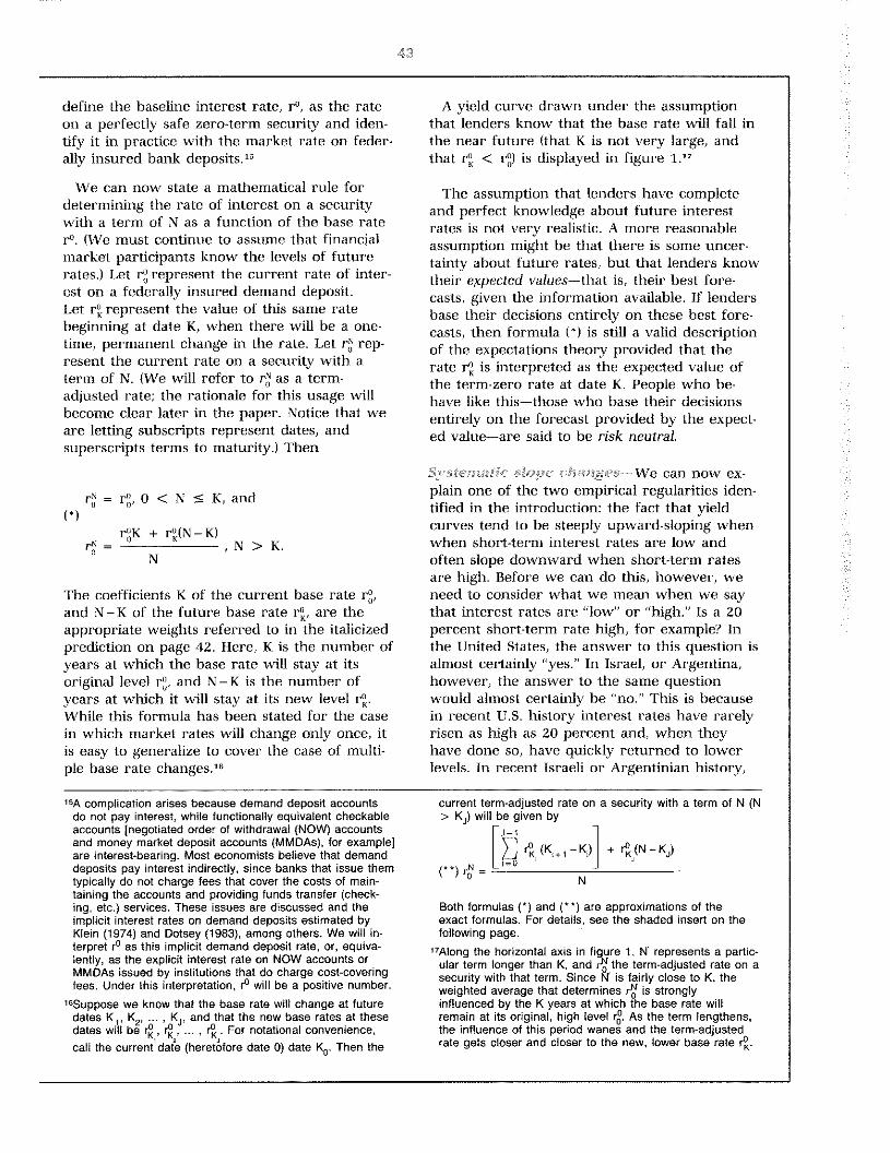
define the baseline interest rate, r°,as the rateon a perfectly safe zero-term security and iden-tify it in practice with the market rate on feder-ally insured bank deposits.”

We can now state a mathematical rule fordetermining the rate of interest on a securitywith a term of N as a function of the base rater°.(We must continue to assume that financialmarket participants know the levels of futurerates.) Let rg represent the current rate of inter-est on a federally insured demand deposit.Let r~represent the value of this same ratebeginning at date K, when there will be a one-time, permanent change in the rate. Let r~rep-resent the current rate on a security with aterm of N. (We will refer to r~as a term-adjusted n-ate; the rationale for this usage willbecome clear later in the paper. Notice that weare letting subscripts rept-esent dates, andsuperscripts terms to maturity.) Then

(*)r~= rg, 0 < N K, and

r~K+ r~(N— K),N>K.

N

The coefficients K of the current base rateand N — K of the future base rate r~,are theappropriate weights referred to in the italicizedprediction on page 42. Here, K is the number ofyears at which the base rate will stay at itsoriginal level rg, and N — K is the number ofyears at which it will stay at its new level r~.While this formula has been stated for the casein which market rates will change only once, itis easy to generalize to cover the case of multi-ple base rate changes.’°

A yield curve drawn under the assumptionthat lenders know that the base rate will fall inthe near future (that K is not very large, andthat r~C rg) is displayed in figure 1.’~

The assumption that lenders have completeand perfect knowledge about future interestrates is not very realistic. A more reasonableassumption might be that there is some uncer-tainty about future rates, but that lenders knowtheir expected values—that is, their best fore-casts, given the information available. If lendersbase their decisions entirely on these best fore-casts, then formula (*) is still a valid descriptionof the expectations theory provided that therate r~is interpreted as the expected value ofthe term-zero rate at date K. People who be-have like this—those who base their decisionsentirely on the forecast provided by the expect-ed value—are said to be risk neutral.

S*•’stnnlat’ln slkIpI.l n1~1an ~ We can now ex-plain one of the two empirical regularities iden-tified in the introduction: the fact that yieldcurves tend to be steeply upward-sloping whenwhen short-term interest rates are low andoften slope downward when short-term ratesare high. Before we can do this, however, weneed to consider what we mean when we saythat interest rates are “low” or “high.” Is a 20percent short-term rate high, for example? Inthe United States, the answer to this question isalmost certainly “yes.” In Israel, or Argentina,however, the answer to the same questionwould almost certainly be “no.” This is becausein recent U.S. histon’y interest rates have rarelyrisen as high as 20 percent and, when theyhave done so, have quickly returned to lowerlevels. In recent Israeli or Argentinian history,

“A complication arises because demand deposit accountsdo not pay interest, while functionally equivalent checkableaccounts [negotiated order of withdrawal (NOW) accountsand money market deposit accounts (MMDA5), for examplelare interest-bearing. Most economists believe that demanddeposits pay interest indirectly, since banks that issue themtypically do not charge fees that cover the costs of main-taining the accounts and providing funds transfer (check-ing, etc.) services. These issues are discussed and theimplicit interest rates on demand deposits estimated byKlein (1974) and Dotsey (1983), among others. We will in-terpret r0 as this implicit demand deposit rate, or, equiva-lently, as the explicit interest rate on NOW accounts orMMDAs issued by institutions that do charge cost-coveringfees. Under this interpretation, r0 will be a positive number.

‘6Suppose we know that the base rate will change at futuredates K,, K

2,..., K~,and that the new base rates at these

dates will be r~,r~,...,r~- For notational convenience,call the current’ dat’e (heretáfore date 0) date l<~.Then the

current term-adjusted rate on a security with a term of N (N> K) will be given by

r~(K~+i_K~)J(**)rN ‘~O

N

+ r~<(N—K~)

Both formulas (*) and (* *) are approximations of theexact formulas. For details, see the shaded insert on thefollowing page.

“Along the horizontal axis in figure 1, N’ represents a partic-ular term longer than K, and the term-adjusted rate on asecurity with that term. Since N’ is fairly close to K, theweighted average that determines is stronglyinfluenced by the K years at which the base rate willremain at its original, high level rg. As the term lengthens,the influence of this period wanes and the term-adjustedrate gets closer and closer to the new, lower base rate r~.

The Exact Formula Linking Short- andLong-Term Rates

Both formula ( ) and the gene ah ed version N ~

presented in footnote 16 are linearized approxi- ~ — (i + r° K - —

mations of the exact formula The exact version 1 K

of formula (1 states that, if rg is the currentbase rate, and r~is the base rate at date K, Fortunately, the approximations given by thethen the current N-pertod term-adjusted rate linearized formulas are adequate for most

satisfies the relation hip purposes. In the case described on pp 42 of

the text, for instance, the yield given by the(1 +r~—u + rg) (1 + ~) , exact formula is 8 743 percent, compared to

the linearized figure of 8-750 percent.

ivhich implies The expectations theory can also be shownto imply that, if r~ms the current N-periodterm adjusted rate and r~is the current

r~= i~Ri+r~r 1 K-period rate then r K, the term adjusted rateon (N — K)-period securities that is expected to

If we know the base rate will change at prevail at date K, satisfies the relationshipfuture dates K K, , K, and that the newbase rates at these dates will be 4, rf( (1+r’ K)’ =

r° [again, for notational convenience, calhngth~ecurrent date (date 0) date K0, and theterminal date (date N) date K ,1 then the which implies thatcurrent term-adjusted rate on a security wmtha term of N (N > K,) satisfies the relationship r~‘= ,f~TTi7~i+~~<i.

(l+r)N= (1+4 The rate K is often referred to as the

“K period forward rate’ on a security witha term of N K. The expectations theory is

[here [J is the multipllcative analogue of I often described as a theory that identifiesthe forward rate with the expected future

This implies spot i-ate.

by n ntrast, rate have rareh fallen as lo~as wIl slope downwai d, and that tt en we expect20 1 en cent and, n hen the~have done so, ha~e them to rise the cut e ts il slope upn ard.

~ klv returned to higher le~e 5. -Ihe simple expectatrons theory has the urtue¼hen ‘a e Sc that intere. I ratr ate high or of gr ea flexihilit~: if so i are ‘a illing to make

Ion, ‘a hat ‘a e u ually mean is that they are sufficiently irtful assumption~about lenders’ cx-high 01 Ion i elatix e to recen historical exper’i- pectatnons ahou the pattern of future in ci est

n ‘e, and that ‘a e te ‘1 this experience gives us n ates, you can use this theor v to explain ti ea good d al of guidance about the les I of inter I tpe of sr’tu tHy any ield cu ye. ‘I he theoryest rate n tl e ft ure. TI us, ‘a bet ‘a e say in pi os-ices an explana(on for one hasc ernpircalter st I aft. are high u e usual v expect them to regula tv tbout yield curt es tha s nat icr dffi-fall in tl e future and ice er, a. \ ‘a e has e cult o helies e, hones er. The regularit in ques-jus set n, th expectations theon s predicts that tion s that most of the i ne, during he lasts hen se expect t-ates to fall the yield curv - centu y at least, it 1 c rves ha p been distinctls

Figure 1Term-adjusted Yield When the Base Rate WillFall in the Future

Yield

upward-sloping.” The simple expectations the-ory could explain this only by assuming thatlenders usually expect rates to rise persistentlyover timne. ‘I’his assumnption does not seem plau-sible, unless you believe that lenders were cx-tremely poor forecasters. While interest rateshave varied considerably during the past centurythere is little evidence that they have increasedon average, or that market participants had anyreason to expect them to do so. Indeed, theevidence suggests that people usually expectfuture short-term interest rates to remain near

current levels. 10 What xve need, then, is amodified version of the theory that will predict

an upward-sloping yield curve under thisassumption.

.hitereat JUçJ-r Tenn i-’ra,nta and

lJteSkj.ie of th.e Vied.! Carve

Any alternative explanation for the fact thatyield curves are normally upward-sloping must

he based on something about long-term securi-ties that makes them systematically less attrac-tive to lenders than short-termn securities. As wehave just seen, the expectations theory predictsthat, if lenders know for’ certain that short-terminterest rates will remain constant, they should

liSee Malkiel (1970), pp. 5-6, 12; Kessel (1965), pp. 17-19;and Shiller (1990), p. 629. It is sometimes asserted thatyield curves were usually downward sloping during the latenineteenth and early twentieth centuries: see Meiselman(1962), appendix C, and Homer and SylIa (1991), pp. 317-22,403-09 for descriptions and explanations of this phenomenon.

“The simple statiscal models of interest rate behavior thatexplain the data best are based on the assumption that

rates have a long-run average or mean level and tend toreturn toward that level, rather slowly, after departing fromit. These models imply that, if short-term interest rates arecurrently near their mean level (where they should be mostof the time), they should be expected to stay near the cur-rent level in both the short and the long run, and that, evenif they are far from the mean level, they should be expectedto stay near the current level in the short run.

r°0

0

K

Current BaseRate I

Future Base RateI I~

0 K N’Term

FRflFriA, RRSRRVr RANK OF ST. LOUiS

be indifferent between lending by purchasingshort-term securities and lending by purchasinglong-term ones. Long- and short-term interestrates should consequently be equal, and theyield curve should he flat. ‘I’his predictionimplies that any alternative explanation for theupward slope of the curve must be based onthe effects of uncertainty about future interestrates.

~-~-ra One reasonwhy uncertainty about interest rates mayinfluence the behavior of lenders is that unan-ticipated changes in interest rates affect the val-ue of their securities in the secondary market.Suppose, to return to an earlier example, that alender buys a 10-year security that returns ayield of 7½percent and sells it in the secondarymarket after five years. If interest rates haveremained unchanged in the interim, the secon-dary market price of his security will give hima five-year yield of 7½percent. If they have ris-en, the price will be lower, and he willreceive a lower yield.

As we have already noted, the reason fon-these price and yield changes is that a securitysold in the secondary market must competewith primary market securities with the sameterm as its remaining term. If the market inter-est rate on primary securities has risen, theyield on secondary securities must rise to thesame level; since the remaining payments onthese securities are fixed, this rise can bearranged only through a decline in the securi-ties’ market price. A formal way to see this isby inspecting the secondary market pricingformula for a single-payment security:

_____ -T

If 4 = 4, so that interest rates have not changedsince this security was issued, its price will be

V. = (1+r~P~~

It is easy to check, by applying the annual inter-est rate formula, that both the T-year cx postyield on this security (the yield from date 0,when it was issued, to date 1’, when it is sold)and the N-T year cx ante yield (the yield fromdate T, when it is sold, to date N, when it willmature) are equal to the initial rate 4.

We will call ~‘-r the anticipated price of thissecurity. If the actual price V~exceeds theanticipated price V1., we say the original lenderhas experienced a capital gain. ‘I’he amount ofthe gain is simply V.r — VT. If the anticipatedprice falls short of the actual price, the lenderhas experienced a capital loss in the amountV1 — Vr It is clear from our pricing formula thatcapital gains occur if r! falls short of 4 (if mar-ket interest rates have fallen), and vice versa.This means that lenders’ expectations aboutfuture capital gains and losses must be tied totheir expectations about future interest rates.

What should we assume about expectationsregarding future interest rates? As we noted to-ward the end of the previous section, it seemsreasonable to assume that market participantsrecognize that interest rates may change, butexpect them to remain constant on average.20

20The expectations theory offers no explanation for thereasons market participants might expect short-term ratesto change. It is a theory that attempts to explain the levelsof long-term interest rates relative to the current levels ofshort-term rates, not one that attempts to explain theirabsolute levels. Stated differently, the expectations theoryis not a true theory of the determination of interest rates.Market participants may expect short-term interest ratesto change because they expect changes in any of theinnumerable factors economic theory predicts mightinfluence them.

Economic theory suggests that interest rates of the sortdiscussed in this article (money or nominal interest rates)are sums of real interest rates (rates expressed in termsof the purchasing power of the dollar amounts lent andrepaid) and expected rates of inflation. This is the so-calledFisher equation. As a result, the question of interest ratedetermination is sometimes thought of as two questions:what determines real interest rates, and what determinesinflation expectations. Most economists believe that nomi-nal factors (such as changes in the levels or growth

rates of monetary aggregates) play the principal role indriving inflation expectations, while real factors (such astechnological changes, changes in the perceived attractive-ness of investment opportunities, changes in demographicstructure or changes in the nature of financial regulation)play the principal role in real interest rate determination.There is, however, considerable disagreement about thedegree of interaction between nominal and real factors, andespecially about whether changes in nominal factors canhave persistent effects on real interest rates.

41

Under this assumption, the expected capitalgains on future secondary market sales of secu-rities are approximately zero.2’

It seems conceivable that this situation mightnot bother lenders. Economists usually assume,howevej, that the satisfaction a person derivesfrom an extra dollar’s worth of expendituresdeclines as the total value of his expendituresincreases. tf this is so, he will find the gain insatisfaction provided by the extra goods he canpurchase if his retuins exceed his expectationsto be smaller than the loss in satisfaction fromthe goods he will have to refrain from purchas-ing if his returns fall short of his expectations.This should cause actuarially fair (zero expectedloss) uncertainty about the future returns onhis securities to upset him. A person whobehaves like this is said to be risk averse.

Since buying terni securities exposes lendersto actuarially fair return uncertainty, while buy-ing securities with zero terms (such as demanddeposits) does not, risk averse lenders will bereluctant to buy term secut-ities. ‘I’hey will insiston higher expected yields on term securitiesthan on demand deposits to compensate them-selves for the uncertainty. The notion thatfinancial decisionmakers are risk averse is wide-ly accepted by economists, and we will adopt itwithout further discussion.

hth’r~,cf014-k anA’ thr, Tar .Ktn1ralrP Wehave just explained why term securities tend tohave higher yields than demand deposits whenboth are default-free: term securities carry in-terest risk, but demand deposits do not. Wehave not yet explained why securities withlonger terms tend to have higher yields thanthose with shorter ones. Our discussion certainlysuggests a possible explanation, however:longer-term securities may carry more interestrisk than shorter-term ones. But why shouldthis he the case?

We will begin our investigation of this ques-tion by posing another question that is closelyrelated. Suppose xve have two single-paymentsecurities with different terms, but the sameoriginal (date 0) prices and yields. If marketinterest rates remain unchanged, their cut-t-ent(date T) prices will also he identical, even

though their maturity payments will not be.But suppose that the market interest rate—specifically, the market “base rate” r°—risesby afixed amount from date 0 to date T (so that 4= rg + Ar, with Ar > 0). Which security willfall furthest in price?

Notice that the remaining term of the short-term security will be smaller than that of thelong-term security; if we call the short term N,,and the long term N1, then the remaining termsof these securities are N, — T and N1 — T, respec-tively. Since market yields have risen, the short-ten’mn secondary security must generate extrainterest to compete with newly-issued short-term securities. The amount of extra interestwill be approximately ArVT(N, — T); this is therate increase Ar, applied to the (common) secon-dary market price VT, for each year of the re-maining term (N, — ‘F). The long-term securitymust also genem-ate extra interest; in this case,the amount is ArV.,.(N1—T). This is the same rateincrease, applied to the same base price, butcontinued for N, — N, additional years.

Of course, neither security can really produce“extra interest” in the conventional sense. Theinterest is paid indirectly, as part of the maturitypayment, and the time and date of that paymentare fixed. Instead, the price of each securitymust decline far enough so that it can increaseat the new (and higher) annual rate 4, whilestill reaching the fixed maturity payment V~atthe maturity date N. Since the price of the long-term security will have to increase at this ratefor a much longer time, it will have to fallmuch further than the price of the short-termsecurity. The relative sizes of the two pt-icedeclines will he approximately equal to therelative sizes of the securities’ remaining terms.A security with four years left to run willsuffer a price decline approximately doublethat of a security with the same secondarymarket price but only two years left to run,and so on.

~11’r~rkNm- If the risk of capital losson securities tends to increase in proportion totheir remaining terms, lenders who demandinterest compensation for bearing this risk willdemand more compensation on long-term

“Since the secondary market price is computed by dividingthe maturity payment by the gross interest rate 1 + r, anincrease in the rate by a given percentage causes a fall inthe price that is slightly smaller than the rise in the pricecaused by an equal percentage decrease in the rate.

As a result, the expected price change is slightly positive.Although this effect is never very strong, it becomes morepronounced as the remaining term of the secondary securityincreases.

securities than on short-term securites.” Thiswill tend to make the yields on longer-termsecurities higher than those on securities withshorter terms—that is, it will tend to make theyield curve upward.sloping.23

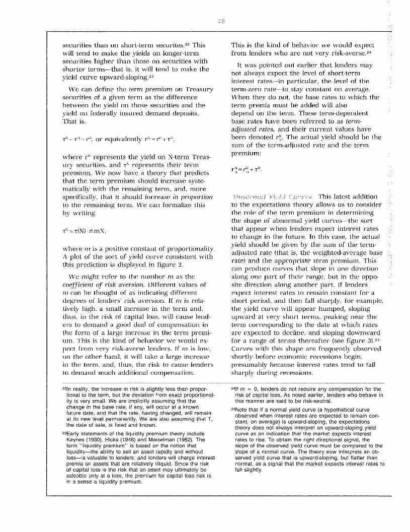
We can define the term premium on Treasurysecurities of a given term as the differencebetween the yield on those securities and theyield on federally insured demand deposits.That is,

TN = rN — r°,or equivalently P’ = r°+ TN

where rN represents the yield on N-term Treas-ury securities, and TN represents their termpremium. We now have a theory that pm-edictsthat the term premium should increase syste-matically with the remaining term, and, morespecifically, that it should increase in proportionto the remaining term. We can formalize thisby writing

T~’=T(N) RmN,

wheme m is a positive constant of proportionality.A plot of the somt of yield curve consistent withthis prediction is displayed in figure 2.

We might refer to the number in as thecoefficient of risk aversion. Different values ofm can he thought of as indicating differentdegrees of lenders’ risk aversion. If m is rela-tively high, a small increase in the term and,thus, in the t-isk of capital loss, will cause lend-ers to demand a good deal of compensation inthe form of a large increase in the term premi-um. ‘I’his is the kind of behavior we would ex-pect from very risk-averse lenders. If m is low,on the other hand, it will take a large increasein the term. and, thus, the risk to cause lendersto demand much additional compensation.

This is the kind of behavior we would expectfrom lenders who are not very risk-averse.”

It was pointed out earlier that lenders maynot always expect the level of short-terminterest rates—in particular, the level of theterm-zero rate—to stay constant on average.When they do not, the base rates to which theterm premia must be added will alsodepend on the term. These term-dependentbase rates have been referred to as term-adjusted rates, and their current values havebeen denoted 4. The actual yield should be thesum of the term-adjusted n-ate and the termpremium:

4 = 4 +

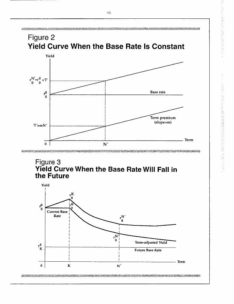
This latest additionto the expectations theory allows us to considerthe role of the term premium in determiningthe shape of abnormal yield curves—the sortthat appear when lenders expect interest ratesto change in the future. In this case, the actualyield should be given by the sum of the term-adjusted rate (that is, the weighted-average baserate) and the appropriate term premium. Thiscan produce curves that slope in one directionalong one part of their range. but in the oppo-site direction along another part. If lendersexpect interest rates to remain constant for ashoit period, and then fall shaiply, for example,the yield curve will appear humped, slopingupward at very short ten’ms, peaking near theterm corresponding to the date at which ratesare expected to decline, and sloping downwardfor a range of terms thereafter (see figure 3).”Curves with l,his shape are frequently ohsemvedshortly hefote economic J-ecessions begin,presumably because interest rates tend to fallsharply during recessions.

“In reality, the increase in risk is slightly less than propor-tional to the term, but the deviation from exact proportional-ity is very small. We are implicitly assuming that thechange in the base rate, if any, will occur at a knownfuture date, and that the rate, having changed, will remainat its new level permanently. We are also assuming that T,the date of sale, is fixed and known.

“Early statements of the liquidity premium theory includeKeynes (1930), Hicks (1946) and Meiselman (1962). Theterm “liquidity premium” is based on the notion thatliquidity—the ability to sell an asset rapidly and withoutloss—is valuable to lenders, and lenders will charge interestpremia on assets that are relatively illiquid. Since the riskof capital loss is the risk that an asset may ultimately besaleable only at a loss, the premium for capital loss risk isin a sense a liquidity premium.

241f m = 0, lenders do not require any compensation for therisk of capital loss. As noted earlier, lenders who behave inthis manner are said to be risk-neutral.

“Note that if a normal yield curve (a hypothetical curveobserved when interest rates are expected to remain con-stant, on average) is upward-sloping, the expectationstheory does not always interpret an upward-sloping yieldcurve as an indication that the market expects interestrates to rise. To obtain the right directional signal, theslope of the observed yield curve must be compared to theslope of a normal curve. The theory now interprets an ob-served yield curve that is upward-sloping, but flatter thannormal, as a signal that the market expects interest rates tofall slightly.

49

Figure 2Yield Curve When the Base Rate Is Constant

Yield

r0__ Base rate

7 =mN Te~ Term

~. . a&wwrar iaavsu.

Figure 3Yield Curve When the Base Rate Will Fall inthe Future

Yield

Term

0

0

r0

K

rN’0

0 K N’

.44

W.NCLUDENG ;0Js’jV414110J4

This article presents a basic description of theconcepts and issues involved in the study of theterm structure of interest rates. It has alsopresented a simple version of the expectationstheory of the term structure. This theory pt-e-dicts that the shape of the yield curve is deter-mined by the expectations of financial marketparticipants about the level of future interestrates and by their uncertainty about theaccuracy of their expectations.

The analysis presented here suggests that theexpectations theory can help explain two impor-tant “stylized facts” about yield curves: the factthat the steepness and direction of their slopestend to vary systematically with the level ofshort-term interest rates, and the fact that theyare usually upward-sloping. The explanation forthe former fact is that forward-looking lenderswill refuse to purchase term securities unlesslong-tetm interest rates are averages of theshort-term interest rates that the lenders expectat various points in the future. The explanationfor the latter fact is that the interest risk onsecurities tends to increase with their terms;this causes risk-averse lenders to demandamounts of interest compensation that alsoincrease with the terms.

Culbertson, John M. “The Term Structure of Interest Rates,”Quarterly Journal of Economics (November 1957),pp. 485-517.

Dotsey, Michael. “An Examination of Implicit Interest Rateson Demand Deposits,” Federal Reserve Bank of RichmondEconomic Review (September/October 1983), pp. 3-11.

Hicks, John R. Value and Capital, 2d ed. (Oxford UniversityPress, 1946).

Homer, Sidney, and Richard Sylla. A History of InterestRates, 3d ed. (Rutgers University Press, 1991).

Kessel, Reuben A. “The Cyclical Behavior of the TermStructure of Interest Rates,” National Bureau of EconomicResearch Occasional Paper #91 (1965).

Keynes, John M. A Treatise on Money, Vol. 1&2 (Harcourt,Brace and Company, 1930).

Klein, Benjamin. “Competitive Interest Payments on BankDeposits and the Long-Run Demand for Money,” AmericanEconomic Review (December 1974), pp. 931-49.

Lutz, Friedrich A. “The Structure of Interest Rates,”Quarterly Journal of Economics (November 1940),pp. 36-63.

Malkiel, Burton G. “The Term Structure of Interest Rates:Theory, Empirical Evidence, and Applications,”Monograph (General Learning Corporation, Morristown,New Jersey), 1970.

Meiselman, David. The Term Structure of Interest Rates(Prentice Hall, Inc., 1962).

Mishkin, Frederic S. The Economics of Money, Banking, andFinancial Markets, 2d ed. (Scott, Foresman and Company,1989).

Modigliani, Franco, and Richard Sutch. “Innovations inInterest Rate Policy,” American Economic Review(May 1966), pp. 178-97.

Russell, Steven H. “Reference Notes on Interest Rates,Securities Pricing, and Related Topics,” Unpublishedmonograph, 1991.

Shiller, Robert J. “The Term Structure of Interest Rates,”(with an appendix by J. Huston McCulloch) in Benjamin M.Friedman and Frank H. Hahn, eds., Handbook of MonetaryEconomics, Vol. 1 (North Holland: Elsevier SciencePublishing Company, Inc., 1990).

Wood, John H. “The Expectations Hypothesis, the YieldCurve, and Monetary Policy,” Quarterly Journal ofEconomics (August 1964), pp. 457-70.