UNIVERSITY OF READING

Department of Meteorology

UNDERSTANDING NEAR-SURFACE

TURBULENCE FLUXES USING AN OPEN-

PATH GAS ANALYSER

Isabella Van Damme

A dissertation submitted in partial fulfilment of the requirement for the degree of Master of Science in Applied Meteorology

August 2010

Acknowledgment

I would like to thank my supervisors, Curtis Wood and Janet Barlow, for their guidance and

useful discussions and for giving me the opportunity to learn more about the fascinating

topic of boundary layer meteorology. The practical aspect of this work would not have been

possible without the assistance of Rosemary Wilson, who installed the instruments and the

equipment needed for calibration, and Ian Reed who never tiered of taking the sensor down

for me, no matter what the weather conditions were. Michael Stroud kindly provided me

with additional data from the Atmospheric Observation site and gave me information about

the practical aspects of different measurement techniques. Most of all, everybody always

welcomed my requests and questions and ensured I had an interesting and enjoyable

project.

Abstract

The concentrations of carbon dioxide (CO2) and water vapour were measured over 9 weeks

on the Atmospheric Observatory at the University of Reading using an open-path gas

analyser (OPGA). Fluxes were estimated from these measurements, combined with data

from a sonic anemometer, using the eddy correlation technique. The instrument

measurement error was 0.30 % on concentrations of CO2 and 1.3 % on water vapour.

Concentrations of CO2 were approximately 30 ppmv higher at night than during the day and

correspond to positive CO2 fluxes at night and negative fluxes during the day. This is

characteristic of a vegetated area and the diurnal variations are related to the atmospheric

boundary layer depth as well as respiration and absorption of CO2 through photosynthesis.

A source area analysis was not inconsistent with gas concentrations and particularly fluxes,

originating mainly from a vegetated area within 100 m from the sensor. The absolute

humidity, as measured with the OPGA, correlated well with results from a psychrometric

measurement and small differences are attributed to the choice of the coefficients used in

psychrometric method. The latent heat flux derived from the eddy correlation method was

up to 8 times smaller than fluxes derived from open-pan, Piche tube or Penman-Monteith

evaporation. The eddy correlation measurements indicate evaporation restricted by

moisture availability, mobility, plant physiology and atmospheric conditions while the other

methods represent unrestricted evaporation. Uncertainties associated with each method

lead to further differences. The hypothesis is put forward that the uncertainty associated

with the eddy correlation method originates mainly from post-field processing. Although

the measurements were carried out in an urban environment, the results are only

representative of the vegetated surroundings within 100 m from the sensor and indicate the

importance of intra-urban variation in surface characteristics as well as the need to select

appropriate measurement locations to obtain results that are representative of the wider

urban environment.

Table of Contents

Chapter 1 : Introduction ........................................................................................................... 1

Chapter 2 : Micrometeorology .................................................................................................. 7

2.1 The atmospheric boundary layer ............................................................................... 7

2.2 Latent heat ................................................................................................................. 9

2.3 Eddy correlation technique ...................................................................................... 12

2.3.1 Theory................................................................................................................. 12

2.3.2 Sources of uncertainty ....................................................................................... 13

2.3.3 Despiking ............................................................................................................ 16

2.3.4 Block averaging .................................................................................................. 16

2.3.5 Coordinate rotation ............................................................................................ 17

2.3.6 Quality control .................................................................................................... 18

Chapter 3 : Experimental work ................................................................................................ 19

3.1 The observation site ................................................................................................. 19

3.2 Open-path gas analyser ............................................................................................ 19

3.2.1 Principle .............................................................................................................. 19

3.2.2 Calibration .......................................................................................................... 21

3.2.3 Sources of measurement errors......................................................................... 22

3.3 Ultrasonic anemometer ........................................................................................... 23

3.4 Additional instrumentation ...................................................................................... 23

3.5 Methods ................................................................................................................... 24

3.6 Data handling ........................................................................................................... 25

Chapter 4 : Results and discussion .......................................................................................... 27

4.1 Sources of uncertainties ........................................................................................... 27

4.1.1 Instrumental uncertainty ................................................................................... 27

4.1.2 Contamination of the windows .......................................................................... 30

4.1.3 Friction velocity as a quality-control measure ................................................... 31

4.2 Diurnal variation in CO2 fluxes and concentrations ................................................. 32

4.3 Water vapour ........................................................................................................... 39

4.3.1 Comparison of absolute humidity measurements............................................. 39

4.3.2 Latent heat fluxes ............................................................................................... 42

Chapter 5 : Conclusions ........................................................................................................... 51

Appendix 1: CO2 concentration and fluxes in Mexico City and London .................................. 56

References ................................................................................................................................ 57

1

Chapter 1: Introduction

Atmospheric concentrations of carbon dioxide (CO2) have increased considerably since the

1950’s and the main cause has been attributed to anthropogenic sources. The absorption by

atmospheric CO2 of terrestrial infra-red radiation creates a greenhouse effect that results in

global average temperature rises (IPCC 2007). Atmospheric water vapour is the most

abundant and dominant greenhouse gas in the atmosphere, as it contributes 60% to the

total radiative forcing compared to 26% for CO2 gas under clear skies, and arises mainly from

natural evaporation of water (Kiehl; Trenberth 1997).

The saturated water vapour increases exponentially with temperature (e.g. according to the

Clausius-Clapeyron equation). This causes a non-linear feedback of water vapour in

response to temperature rises caused by other sources. Evaporation responds

instantaneously to changes in temperature and other atmospheric conditions and any

changes affect the hydrological cycle, which in turn influences cloud formation and the

ecosystem and leads to further climate feedbacks. A growing population and changing

lifestyles impact the landscape. Urban areas continue to expand, often at the cost of

surrounding agricultural land, while forests and other native landscapes are converted to

agricultural use to meet the increasing food production requirements. Changes in land use

alter the carbon cycle and the Bowen ratio (the ratio between sensible and latent heat

fluxes) (Baldocchi et al. 2001). Because of the tremendous impact of CO2 and water vapour

on Earth’s climate and ecosystem, and the chain of feedback mechanisms associated with

that, it is essential to continuously monitor the concentration of these greenhouse gases in

the atmosphere and understand their exchange between the surface and the atmosphere in

a variety of environments.

CO2 and water vapour are produced as by-products of fossil fuel burning and urban areas are

therefore major sources. Plants use CO2 and water vapour, together with light, to grow

through the process of photosynthesis. At night, CO2 and water vapour are released in a

process called respiration (Oke 1995). The CO2 exchange with the ecosystem has been

studied for many years with a range of techniques. The eddy covariance method, based on

the measurement of three-dimensional wind vectors and CO2 densities, is particularly

suitable as it can be used to study the CO2 exchange of the whole environment while

traditional methods are limited to exchange in small areas of leafs, plants or soil (Baldocchi

2

2003). The CO2 flux measurements over vegetation based on eddy covariance have been

applied since the late 1950’s and have developed into a global network linked in the

FLUXNET program (Baldocchi et al. 2001) which currently includes over 500 measurement

sites around the globe. Only in the last 10 years have these measurement techniques been

applied to study the exchange in urban environments. Previously, urban CO2 fluxes were

derived from the estimates of emissions and sequestration (Grimmond et al. 2002). Long-

term measurements of CO2 fluxes in urban environments are particularly relevant since the

main causes of increased [CO2] are associated with fossil fuel burning and changes in land

cover (IPCC 2007) with urban environments being a main source for both. In addition, rural

environments may be affected by advection from urban areas (George et al. 2007; Nemitz et

al. 2002; Rigby et al. 2008) .

The spatial variability of surface cover and roughness in urban areas poses particular

challenges to carry out studies representative of the whole urban area. The choice of spatial

and vertical location of the measurement equipment affects the measurements and

researchers often use multiple urban sites to cover a variety of urban environments (Offerle

et al. 2006). Measurement instruments must be placed in uniform areas at a height at least

double the height of the roughness elements and ideally above the roughness sublayer to

achieve a representative response of the local environment (Grimmond et al. 2002).

CO2 in urban environments

Studies of CO2 concentrations and fluxes in urban environments show large diurnal

variations. Similar trends were found in Chicago (Grimmond et al. 2002), Marseille

(Grimmond et al. 2004), Baltimore (George et al. 2007), London (Helfter et al. 2010; Rigby et

al. 2008) and Mexico City (Velasco et al. 2009) where the lowest concentrations are found in

the afternoon. This is associated with photosynthesis and especially the effective dispersion

of gasses in the daytime boundary layer aided by turbulent mixing. The greatest

concentrations of CO2 are measured during the night and in the morning. This is attributed

to night-time respiration from plants, a relatively shallow boundary layer and reduction of

turbulent mixing in the stable night-time atmosphere. An early-morning maximum is

associated with the morning rush hour when the deep boundary layer is not yet established.

The evening rush hour peak is often not observed and is explained by turbulent mixing and a

3

deeper boundary layer later in the day. Measurements in Essen determined that 71% of the

near-surface [CO2] is affected most by traffic density and atmospheric stability (Henninger

2008). Different weekend effects are observed with lesser concentrations during the

weekend in Baltimore but the greatest concentrations in Mexico City are observed on

Saturday. Here, the morning peak is greater on Saturdays and Sundays than during the

week and is attributed to the return home by night-time revellers, referred to as ‘the party

effect’. Nemitz et al. (2002) found in Edinburgh that traffic was the major source of CO2 but

wind speed and direction also play a role: low wind speeds lead to greater concentrations

while maritime wind and wind from sectors with parkland and residential areas decreased

the concentration.

Seasonal variability with greater CO2 concentrations during the winter in Florence (Matese

et al. 2009) were attributed to the use of domestic heating. The seasonal cycle in London

could be explained by changes in the hemispheric background level of [CO2], heating during

the winter and exchange by the biosphere, not only in London but in an area larger than

London. The meteorological conditions also played a role (Rigby et al. 2008).

In urban environments, CO2 fluxes remain positive throughout the day and urban

environments can be considered a net source of CO2. CO2 fluxes in Chicago did not show

diurnal variations while the largest emissions in Edinburgh, Marseille, Florence, London and

Mexico City were measured during the day. Similar to CO2 concentrations, diurnal variations

in CO2 fluxes in London were also found to be correlated with traffic while seasonal

variations were correlated with heating systems during the winter and photosynthetic

activity (Helfter et al. 2010; Rigby et al. 2008). Strong seasonal variations in CO2 fluxes were

also observed in Helsinki (Jarvi et al. 2009): large negative CO2 daytime fluxes, similar to

those observed over a beech forest, were measured when air temperatures exceeded 12°C.

The magnitude of the positive daytime fluxes increased as the air temperature decreased. In

all the above cases, the magnitude of the fluxes was found to be dependent on wind

direction.

Water vapour

Despite the importance of water vapour as a greenhouse gas and the role of latent heat

fluxes in potentially moderating urban heating effects, only three of the above mentioned

4

urban studies refer to water vapour. George et al. (2007) found that the relative humidity is

the same in urban and nearby rural areas but the absolute humidity is higher in urban areas

since the temperature is higher. In Edinburgh (Nemitz et al. 2002), latent heat fluxes are

positive during the day and make a substantial contribution to the energy budget. The sum

of the latent heat and sensible heat fluxes was larger than the measured net radiation,

which hence suggests an additional heat input from the urban environment. Several studies

of the heat fluxes in North-American cities, Marseille and Lodz covering a range of urban

environments and climatic conditions, identified an inverse relation between the Bowen

ratio and the amount of vegetation (Grimmond et al. 2002; Grimmond et al. 2004; Newton

et al. 2007; Offerle et al. 2006). Flux partitioning as a consequence of variation in intra-

urban surface characteristics can affect the local climate and cause phenomena such as the

park breeze, when air flows from open vegetated areas to surrounding build-up areas as a

result of temperature differences between the two areas (Thorsson; Eliasson 2003). The

effect of climate is complex and temperature and humidity alone are not an indicator for the

energy fluxes as demonstrated in Miami (Newton et al. 2007). Although the climate was

subtropical, the latent heat flux and Bowen ratio are not dissimilar to those found for cities

in temperate climates and is attributed to heat storage in open water and wet soil, low

vapour pressure deficit and low coupling between the surface and the boundary layer due to

a relatively low roughness length in Miami.

Over vegetation, CO2 and water vapour fluxes are linked as photosynthesis and transpiration

occur through the same plant stomata. Changes in stomata density and stomata resistance

affect both fluxes.

Near-surface water vapour originates from evaporation which depends on meteorological

conditions, type of vegetation, surface cover and the amount of water available (Arnell

2002). Still air easily becomes saturated and prevents further evaporation. Turbulence

encourages evaporation by continuously removing the water vapour away from the surface.

Evaporation has long been studied in the context of the water balance, employing a range of

measurement techniques but is considered the most difficult component of the water

balance to measure (Arnell 2002). Several techniques are used but the open-pan

evaporation is one of the most popular since it is cheap and easy to use. Due to the difficulty

in measuring evaporation, mathematical equations are often used to estimate evaporation.

5

Many equations are empirical while others rely on meteorological observations. The

Penman-Monteith equation to estimate potential evaporation is most widely used, for

example in modelling of evaporation in climate models and estimating evaporation for

irrigation purposes recommended by the UN Food and Agriculture Organisation (Arnell

2002; FAO 1998).

Measurement techniques

Continuous and simultaneous measurements of CO2 concentrations ([CO2]) and water

vapour can be carried out with a closed or open-path gas analyser (OPGA) and both have

advantages and disadvantages. Fluxes can be estimated, using the eddy covariance

technique, when these instruments are combined with a fast-response anemometer that

measures the three-dimensional wind vectors. A closed-path analyser requires a pump and

associated tubing to suck in the air to be analysed. This introduces a delay and must be

corrected for to relate the measurements with the instantaneous wind vectors. Further

corrections must be applied because the interaction with the tubing may cause high

frequency losses (Aubinet et al. 2000). The pump installation needs additional maintenance

and the whole system requires frequent calibration but the advantage is that calibrations

can be carried out in-situ and can be automated. Open-path analysers measure the gas

densities directly and require less-frequent calibrations. These calibrations require human

interventions and introduce periods of at least one hour when data are not collected. Open-

path analysers can suffer from environmental contaminations resulting in the rejection of

large numbers of unreliable data.

Project aims

The aim of this project is to evaluate the performance of an open-path CO2/H2O analyser in a

suburban environment and identify possible causes of uncertainty. The calibration drift will

be assessed with the aim to recommend a calibration interval. Of particular interest is the

instrument performance in the presence of rain, dew or fog since these weather conditions

are common in the UK. The results will be compared with data from other meteorological

measurements taken on the same site to validate the measurements or identify possible

reasons for observed differences. This work will particularly concentrate on the comparison

6

of different measurements of absolute humidity and latent heat fluxes. In addition, the

diurnal variations of CO2 concentrations and fluxes will be studied and compared to other

urban sites. Green spaces in urban environments could play an important role for the

overall urban carbon, heat and water vapour fluxes. The exchange of moisture and CO2 by

the vegetated soil together with the transpiration, photosynthesis and respiration by plants

create a completely different environment from the impermeable, heat absorbing/emitting

build environment associated with the urban heat island. The study site, which is

surrounded by a variety of vegetation within an urban area (see later), will enable us to

investigate this.

7

Chapter 2: Micrometeorology

Micrometeorology deals with small-scale processes that occur in the atmospheric layer next

to Earth’s surface, i.e. the atmospheric boundary layer and more specifically, the surface

layer. The transport of energy and mass is a main topic of interest. The following chapter

describes the structure of the atmospheric boundary layer and measurement techniques

used in micrometeorology.

2.1 The atmospheric boundary layer

The atmospheric boundary layer is the layer formed as a consequence of the interaction

between the atmosphere and Earth’s surface. It is the layer where the exchange of mass,

heat and momentum occur. As a consequence, there is a diurnal variation in the structure of

the boundary layer. After sunrise, there is a continuous receipt of downwelling shortwave

radiation, usually resulting in a positive net radiation and thus heating of the surface,

creating buoyant thermal plumes and a well-mixed vertical layer. This daytime unstable

boundary layer grows through encroachment or entrainment reaching a height of 1 to 2 km

(in temperate latitudes) in the late afternoon (Foken 2008). Turbulent mixing is reduced as

a result of the radiative cooling of the surface becoming dominant in the evening and night.

Accordingly the boundary layer takes a new stable form and tends to shrinks to depths of 30

to 300 m in temperate latitudes.

The daytime boundary layer can be sub-divided in several layers (Figure 1). The layer

immediately next to the surface is the roughness sublayer (RSL). Air flows around the

roughness elements, i.e. individual obstacles such as trees, buildings and grass. This layer is

typically 2 to 5 times the mean height of the obstacles. The next layer, the surface layer,

comprises both the RSL and air above, reaching to about 10% of the height of the boundary

layer (Figure 1). In this layer, heat, wind and humidity change rapidly with altitude while

vertical fluxes vary by less than 10%. The near-constant fluxes enable flux measurements

within the surface layer to be related to surface fluxes. Surface heating during the day

causes a decrease of temperature and absolute humidity with height in the surface layer

leading to an unstable surface layer. Under these conditions, heat and vapour

8

Figure 1: Evolution of the structure of the daytime and night time boundary layers (Diagram copied from http://www.smhi.se/sgn0106/if/FoUp/us/html/parameterization.html. Note: the diagramon this web site is incorrectly attributed to Wyngaard, J., confirmed through personal communication with J. Wyngaard. The original source of the diagram could not be located but the diagram is include here anyway because it give a clear overview of the boundary layer structures. )

are transported vertically by eddy diffusion and the resulting convection leads to upward

(positive) sensible and latent heat fluxes. The ratio of sensible to latent heat, the Bowen

ratio, depends on the availability of moisture. Similar reasoning can be applied to the

transport of other substances, such as CO2. The direction and magnitude of the turbulent

transport of the gas molecules depend on the concentration gradient near the surface.

Small (a few mm), high-frequency eddies are found near the surface and these gradually

increase in size with altitude. The well-mixed layer extends from the surface layer to the top

of the boundary layer and occupies most of the volume in the daytime boundary layer

(Figure 1). Turbulence ensures that potential temperature, momentum and scalars are well-

mixed and constant with height, while fluxes decrease with height. Large eddies dominate

this layer and eddies with a diameter equal to the height of the boundary layer can reach

down to the surface. The convective boundary layer is capped by a capping inversion with a

thickness of approximately 10% of the boundary layer (Figure 1). This temperature

9

inversion inhibits further vertical mixing keeping most tracers, such as pollution, within the

boundary layer.

Under idealized conditions (such as cloud-free rural), throughout the evening and night,

stable atmospheric conditions prevail while turbulence and vertical movement is

considerably reduced. The lack of vertical transport of fast moving upper air to the surface

means that nocturnal wind speeds near the surface are often less than during the day. The

dominance of radiative cooling of the surface can lead to a temperature inversion which

results in a downward (negative) sensible heat flux. Negative latent heat fluxes can occur

when the air temperatures drops down to the dew point temperature. A residual mixed

layer exists at higher levels, which is less turbulent than the daytime well-mixed layer, and is

capped by a capping inversion (Figure 1).

In analogy with the above description, an urban boundary layer develops over cities and

affects areas downwind. An internal boundary layer is created by the difference in surface

roughness and surface characteristics compared to a rural area (Oke 1995). Turbulence near

the surface depends on the height of buildings and the width of the streets, while sensible

heat fluxes are affected by the nature of the materials used in towns as well as the density of

the buildings. Water vapour originates from burning of fossil fuels, rivers, parks and water

for home, industrial and leisure use. The dearth of large areas of vegetation and the

impermeable nature of the building materials means that water storage is less than in rural

areas. The shortage of water to evaporate has a major impact on the urban climate since

the net radiation is primarily used to generate sensible heat fluxes and increase urban

temperatures and boundary-layer depths (Oke 1995). The concentration and fluxes of

pollutants and gasses, including CO2, are related to the atmospheric stability and structure,

the meteorological conditions as well as the available sources and sinks. CO2 is a long-lived,

chemically stable greenhouse gas and is only removed from the atmosphere through

photosynthesis by plants or absorption in the oceans over a decadal timescale (IPCC 2007).

2.2 Latent heat

Latent heat fluxes (FE) describe the vertical transport of water vapour taking into account the

heat required to evaporate the water from the surface

10

''qwFE (1)

where is the latent heat of evaporation in J kg-1, w’ is the vertical wind fluctuations in m s-1

and q’ is the fluctuation in absolute humidity in kg/m3. Evaporation of water depends on

the availability of moisture at the surface, the properties of the underlying surface, the

availability of energy to vaporise the water and turbulence to transport the vapour (Arnell

2002). Evaporation from soil depends on capillary transport of moisture to the surface and

depends on the soil type and texture. Evaporation is strongest during the day, when most

energy is available but can continue at night. Water vapour released by plants as part of the

photosynthesis process is called transpiration. Transpiration is related to CO2 exchange by

plants as both are controlled by photosynthesis and occur through the same stomata on

plant leaves. The combination of evaporation and transpiration is often referred to as

evapotranspiration.

The most popular measurement technique to measure evaporation is the open pan

evaporation. It is simple and cheap and is widely used by hydrological and meteorological

agencies (Arnell 2002). This technique is known to have high levels of uncertainty as water

can splash out, animals can drink from it, objects can fall into the pan and there are

inaccuracies associated with reading small differences in water level. Moreover, energy can

be stored in the water for later evaporation. The Piche-tube evaporation (see 3.4)

overcomes some of these problems as it is measured in a Stevenson screen. Both methods

measure evaporation from a water surface, which is unconstraint and is not representative

of a land-based environment. Evaporation is measured in mm water evaporated during a 24

hour (86400 s) period and converted to latent heat flux

86400/wE hF (2)

where is the latent heat of evaporation in J kg-1, h is the depth of evaporated water in m

and w is the density of water in kg m-3. Compared to open water, evaporation over land is

modified by the availability of moisture, the soil type and ground cover. The ground cover is

important as it affects evaporation through its albedo and porosity. Urban environments

consist of large areas of impermeable and often dark surfaces. Large latent heat fluxes can

therefore be expected after rain showers but low fluxes during dry periods as the surface

stores and transmits little water. Anthropogenic sources of water vapour in the urban

11

environment are a by-product of fuel burning. In parks and rural environments, the type of

vegetation also affects the albedo as well as turbulence. High levels of turbulence promote

better mixing and less resistance to transfer of moisture. The resistance to turbulent

diffusion is expressed as aerodynamic resistance ra (s m-1) and is inversely related to

windspeed and vegetation height (Monteith; Unsworth 2001)

*

]}/){ln[(]}/){ln[( 0

2

2

0

ku

zdz

uk

zdzra

(3)

where z is the measurement height, d is the zero-plane displacement height, z0 is the

aerodynamic roughness length, k is the von Karman constant, u is the wind velocity at height

z and u* is the friction velocity. This equation is only valid in neutral stability conditions.

Short grass has a higher aerodynamic resistance than tall trees, i.e. turbulent diffusion from

trees is easier than from grass. Values of ra over short grass range typically between 70 –

200 s/m for windspeeds between 5 and 1 m s-1. Transpiration of water from plants occurs

through stomata on leaves and stomatal resistance expresses the resistance to vapour flow

through the stomata. The stomatal resistance increases at high temperatures and in the

absence of soil moisture. Surface resistance rs (s m-1) describes stomatal resistance together

with resistance of vapour to flow through soil, in case not all the soil is covered by plants

(FAO 1998)

active

ls

LAI

rr (4)

where rl is the stomatal resistance of an average leaf (s m-1) and LAIactive is the leaf area index

and is a dimensionless unit that expresses the leaf area per area of soil underneath it. For a

well-watered crop, rs varies between 100 to 25 s m-1 as the leaf area increases. The surface

resistance is specific for each plant variety and depends on the growth stage of the plants

and the plant density.

The aerodynamic resistance, surface resistance, available energy and vapour pressure deficit

are used in the Penman-Monteith equation to estimate potential evaporation (Monteith;

Unsworth 2001)

)]/1([

/)()(

as

aspan

Err

reeCGRQ

(1)

12

where Rn is net radiation, G is the soil heat flux, a is mean air density at constant pressure,

Cp is the specific heat of the air, es is the saturated vapour pressure, e the vapour pressure,

is the slope of the saturated vapour pressure-temperature relationship and is the

psychrometric constant. The Penman-Monteith equation estimates potential evaporation

and does not represent true evaporation as assumptions are made that the soil is saturated

with water, plant roots can freely extract water and atmospheric conditions do not hinder

evaporation. Changes in turbulent conditions are not accounted for.

2.3 Eddy correlation technique

2.3.1 Theory

The eddy correlation method, also called the eddy covariance method, is used to measure

fluxes. Fluxes, caused by turbulent mixing, are a function of the vertical transport by eddies

of a concentration of a variable (Kaimal; Finnigan 1994) and can be derived from regular and

frequent measurements over time at a fixed observation point. The assumption is made

that Taylor’s frozen turbulence hypothesis is valid, i.e. the observed fluctuations over time at

a fixed point are associated with the advection of turbulence transported by the mean wind.

Turbulence at a point fluctuates, depending on the frequency of the eddies, and vertical

transport is only achieved if fluctuations in the vertical wind velocity correlate with

fluctuations in the variable of interest. The assumption is made that vertical transport is

proportional to the gradient of the mean variable. Reynolds’ decomposition is used to

separate the fluctuation X’ at a time point from the time-mean value of X as

'XXX i

(2)

where Xi is the instantaneous value of a variable. The overbar indicates a time-average and

a prime represents a fluctuation from the mean. The flux FX is expressed as the covariance

between the fluctuations in the vertical wind component w’ and the fluctuations in a

variable X’, such as water vapour, CO2 or temperature, and is generally expressed as

'' XwFX (7)

Positive fluxes indicate a net transport to the atmosphere and negative fluxes denote

transport towards the surface.

13

2.3.2 Sources of uncertainty

The eddy correlation method assumes that (i) the atmosphere is turbulent, (ii) advection is

negligible, i.e. steady-state conditions prevail, and (iii) the terrain is flat and homogeneous.

This implies that the mean vertical flow is assumed to be zero and vertical transport is only

caused by turbulence. Uncertainty due to advection can be reduced by selecting the

appropriate averaging time. Uneven terrain can be accounted for by coordinate rotation.

Errors also originate from spikes in the data and consequently the method used to remove

the spikes and fill in such missing data. The time period selected to average the fluctuations

adds further uncertainty. Coordinate rotation, block averaging, despiking and quality control

will be discussed in more detail in the following sections.

In addition to the causes of uncertainty listed above, many other parameters are reported in

the literature and by the instrument manufacture that can affect flux measurements and

relate to instrumentation, data handling or the flow itself. Eddy correlation measurements

require substantial post-field data corrections but there is no general agreement amongst

micrometeorologist on how best to compute near surfaces fluxes (Mahrt 2010). However, it

is recognised that more effort is needed to identify and quantify the uncertainties associated

with flux measurements (Richardson et al. 2006). The total error is a composite of all

measurement errors and is expressed as random and systematic errors. It is beyond the

scope of this work to give a detailed and comprehensive analysis of all the possible sources

of errors. A brief overview is given of some parameters while Table 1 gives a summary of

sources of errors to highlight the origin of uncertainty associated with flux measurements

using the eddy correlation method and the proposed corrections. The additive effect of the

individual errors could lead to errors of more than 100%. The sources of errors listed in

Table 1 mainly refer to systematic errors. A study of random errors by Richardson et al.

(2006) identified that the magnitude varies depending on season, wind speed and net

radiation. Average random errors up to 3.7 µmol s-1 m-2 in CO2 flux and 26 W m-2 in latent

heat flux were reported although errors up to 170 W m-2 were recorded when the net

radiation was higher than 400 W m-2. In most cases, there are several options for how to

correct and process the data and errors are also inherent in the applied corrections. For a

30-minute averaging method, different methodologies can result in a 10% deviation on

14

sensible heat fluxes and 15% on latent heat fluxes (Mauder et al. 2007). Errors associated

with instrument calibration, maintenance and hardware are not considered here.

Table 1: Sources of errors related to flux measurements derived from an open-gas analyser using the eddy correlation technique

Error Source Error Range (%)

Correction Reference

Instrument installation Optimize installation (Foken 2008)

Sensor separation Spectral correction in the high fre-quency range

(Foken 2008)

Frequency response 5 - 30 Frequency response corrections (Burba; Anderson 2007)

Time delay 5 - 10 Adjust for delay (Burba; Anderson 2007)

Digital sampling error Digital sampling correction (Burba; Anderson 2007)

Loss of flux due to path/volume averaging

Correction factor (Burba; Anderson 2007)

Spikes 0 - 15 Spike removal (Burba; Anderson 2007)

Unlevelled instrument and flow

0 - 25 Coordinate rotation (Burba; Anderson 2007)

Density fluctuations 0 -50 Webb-Pearman-Leuning Correction (Foken 2008)

Sensor heating of gas ana-lyser

Correction factor (Jarvi et al. 2009)

Sonic heat error 0 -10 Sonic temperature correction (Burba; Anderson 2007)

Band Broadening 0 - 5 Band broadening correction (Burba; Anderson 2007)

Missing data filling 0 - 20 Different filling strategies (Burba; Anderson 2007; Foken 2008; Moffat et al. 2007)

Instrument temperature fluctuations

Apply temperature control (Burba; Anderson 2007)

Data averaging Appropriate time scale

Ogive correction

(Finnigan et al. 2003; Mahrt 2010)

Loss of low frequency tur-bulence

Cospectral analysis and high pass filter

(Burba; Anderson 2007; Kaimal; Finnigan 1994)

Loss of high frequency tur-bulence

Cospectral analysis and low pass filter

(Burba; Anderson 2007)

Weak wind , low turbu-lence, storage, advection, stationarity

Apply a u* filter

Stability and non-stationarity tests and corrections

(Finnigan 2008; Foken 2008; Mahrt 2010)

Sonic temperature mea-surements conversion to actual temperatures

Apply correction factor (Foken 2008)

Deviation from Gaussian distribution (skewness, kur-tosis)

Use appropriate statistical methods (Richardson et al. 2006)

Measurement errors can be limited by optimising the instrument installation to avoid any

interference with the measured properties. To prevent distorting the flow, the gas analyser

should be downwind from the sonic anemometer at a horizontal distance of 20 - 30 cm

according to Foken (2008a) but only 10 – 15 cm according to (Burba; Anderson 2007). A

sensor separation error still occurs in the covariance because the two instruments do not

15

measure at the same point in space (Burba; Anderson 2007). It is also recommended to

install the open-path analyser at or slightly below the sonic anemometer (Burba; Anderson

2007; Grelle; Burba 2007). Distortion of the vertical wind component can be reduced by

keeping the area and mast underneath the instruments clear. The measurement height

should be 2 to 5 times the canopy height and 5 to 18 times the instrument path length

(Burba; Anderson 2007). The instrument sampling rate must be sufficiently fast to include

even the smallest turbulent scales of motion and concentration fluctuations. Sources of

instrument error are reviewed in section 3.2.3.

The open-gas analyser measures gas densities in mmol per unit volume. Fluctuations in

pressure, temperature and water vapour result in changes in the volume, i.e. the air density,

and affects fluxes of CO2 and water vapour. The Webb, Pearman and Leuning (WPL)

correction (Webb et al. 1980) is usually applied although there is continuing discussion over

the validity of this correction (Foken 2008). The correction is dependent on the heat and

evaporation fluxes, the density of the measured gas and the air temperature. This means

that corrections of water vapour fluxes for changes in air density include the magnitude of

the water vapour flux itself in the calculations of the correction. The correction step must

therefore be iterative but this is not reported in the literature. Effects of pressure

fluctuations are not included in the WPL correction and it requires accurate values of heat

and evaporation fluxes. Further corrections are required because the open-path analyser

itself generates heat and affects the measurement volume. The sensible heat flux in the

optical path caused by electronic heating and radiation can be measured with a fine-wire

thermometer and should be used in the WPL equation instead of the ambient sensible heat

(Burba et al. 2008; Grelle; Burba 2007). The sensible heat flux in the optical path has been

reported to be up to 14% higher than the ambient heat flux (Burba et al. 2008). However,

this is only valid if the gas analyser is installed near-vertically. Compared to a closed-path

analyser, where the WPL correction need not be used, applying the standard WPL correction

can still lead to an underestimation of the CO2 flux by 19% while including the instrument

heating correction reduced this error to only 4% (Grelle; Burba 2007). The WPL density

correction is small during the growing season and large in winter when CO2 fluxes are small

(Burba; Anderson 2007). The lack of energy balance closure reported for near-surface flux

measurements using the eddy correlation method suggest that the energy fluxes are

16

underestimated and this will affect the accuracy of the WPL correction (Jarvi et al. 2009;

Wilson et al. 2002a). In addition, random errors on the energy fluxes can be substantial

(Richardson et al. 2006). Because of the large uncertainties on the parameters used in the

WPL correction and since the measurements reported in this work were taken during May to

July, the WPL correction will not be applied to the analyses presented in this dissertation.

The analysis of the WPL correction is included here as an example to illustrate that

corrections applied in response to errors in the eddy correlation method may not completely

rectify the errors and can even introduce further uncertainties. Due to time restrictions of

this project, only the corrections discussed in the next sections were applied in this project

as these were considered to be the most important.

2.3.3 Despiking

Spikes can be caused electronically but one of the major sources of errors in data from an

open-path gas analyser is caused by interference of particles or droplets in the optical path

of the instrument. Since the path is exposed to the environment, any object crossing the

path is registered as a spike. Precipitation, insects, pollen and dust passing through the path

cause temporary interference. The open-path gas analyzer sequentially rotates between

different wavelengths and any temporary obscuration may affect only one of the

wavelengths leading to a large difference, seen as a spike, between the absorption of the

reference and measurement wavelengths. The manufacturer claims that deposition on the

measurement window equally affects all wavelengths as long as the objects are stationary

and should not cause spikes. Some applications require continuous data sets and it is

therefore common practice to fill in missing data (Baldocchi et al. 2001). Different methods

can be used to eliminate spikes and replace the data (Goring; Nikora 2002). Spike

elimination is commonly based on removing data points that deviate by a multiple of the

standard deviations from the mean value. Many methods can be used for gap filling (Moffat

et al. 2007) but the most simple and commonly used methods use the average of the

nearest points, linear or non-linear interpolation or use averaged long term or

meteorological values.

2.3.4 Block averaging

Reynolds’ decomposition and flux calculations involve taking the arithmetic mean over a

certain time period. The time-scale chosen must be long enough to encompass the

17

frequency spectra of turbulences that will be encountered but not too long to avoid

including synoptic changes, advection and diurnal variations. The ability to measure high

frequency eddies is only determined by the sampling rate of the instruments and is not

affected by the choice of averaging time. The size of the smallest eddy that can be

measured is determined by the optical path length of the open-path gas analyser. A

sampling rate of 10 -20 Hz for near-surface measurements is suggested (Foken 2008). As

the optimum averaging time is dependent on the atmospheric stability and wind velocity, a

shorter averaging time can be used during the day and a longer time is required at night.

Although the appropriate averaging time is dependent on the local conditions and

measurement height, an averaging time of 30 min for near-surface measurements is

generally recommended (Foken 2008; Kaimal; Finnigan 1994). This time scale is sufficiently

long to encompass the turbulence representing the whole frequency spectrum, including

two or three large eddies. Under some circumstances it may be necessary to average over

longer time scales, especially over complex terrain and in a stable atmosphere (Finnigan et

al. 2003). Low values of fluxes, leading to a lack of energy balance closure, have been partly

attributed to the omission of low frequency turbulence and averaging times of 4 hours may

be required (Finnigan 2008).

2.3.5 Coordinate rotation

Eddies are transported horizontally with the mean wind in the horizontal plane and the

assumption is made that the mean vertical wind is negligible. The measurement of fluxes is

based on measuring fluctuations in transport vertical to the horizontal plane. The sonic

anemometer measures wind vector components relative to the orientation of the

instrument. The true vertical velocity is not measured due to tilting of the vertical

instrument axis and the horizontal wind may be distorted by the underlying terrain. This can

be corrected for by applying a correction. This involves rotating the x, y, z coordinate system

to align the x-axis with the mean wind vector. Several methods have been proposed to

calculate the tilt correction (Wilczak et al. 2001). The method applied in this work consists of

a double rotation of the anemometer axis. The sonic anemometer gives wind components

u, v, w in a right-handed coordinate system x, y, z. The first rotation rotates the coordinates

through and angle α around the z-axis so that the mean wind component v is zero. The

second rotation rotates the coordinates through an angle β around the y-axis and the mean

18

wind vector w is zero. The coordinate system is now aligned with the streamlines and the

new wind vector components u2, v2 and w2 relate to the mean sonic wind components

w

v

u

w

v

u

cossinsinsincos

0cossin

sincossincoscos

2

2

2

(8)

with )/arctan( uv and )arctan( 22 vuw . A third rotation is sometimes applied

to make the covariance between the w’ and v’ equal to zero. This third rotation is usually

very small and can even produce unphysical results (Finnigan et al. 2003). It is therefore

recommended only to apply the first two rotations and try to align the vertical anemometer

axis as close as possible perpendicular to the surface.

2.3.6 Quality control

The quality control step allows the removal of obviously-bad data. The most common

causes of bad data are related to precipitation and atmospheric conditions. Although spikes

have already been removed, the effect of precipitation or dew can still be seen in the

processed data as obviously-bad data points. In this work, data affected by precipitation

were removed based on a diagnostic value given by the open-path gas analyser.

Stable atmospheric conditions often occur at night. Wind speeds and turbulence can be

small and fluxes negligible while advection, storage near the surface and in the canopy as

well as drainage become important (Finnigan 2008). Data obtained under these conditions

are not an accurate measure of the exchange between the surface and the atmosphere and

result in an under-estimation of night time CO2 fluxes. Water vapour fluxes are not affected

since these are close to zero during the night (Baldocchi et al. 2001) . Several tests for

quality control purposes can be used (Aubinet et al. 2000; Baldocchi et al. 2001; Foken 2008;

Vickers et al. 2010). A commonly used criterion is to remove data that correspond to low u*

values. There is no general agreement on threshold level and the choice of threshold of u*

is based on the judgment of individual researchers and on the local conditions. Threshold

values of u* ranging between 0.02 and 0.86 m s-1, depending on the site and time of year,

have been suggested (Gu et al. 2005).

19

Chapter 3: Experimental work

3.1 The observation site

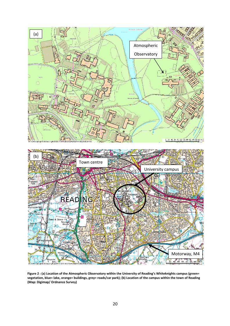
Observations were taken at the Atmospheric Observatory at the University of Reading

(51.44’N, 0.938’W, 66 m above mean sea level). The site is approximately 2 km to the south-

east of the centre of Reading and 2.3 km to the north of the M4 motorway (Figure 2). The

nearest public road is approximately 240 m to the East. The instruments are installed over a

grassy surface. The site is in an open area surrounded by extensive and diverse vegetation

interspersed with buildings and a small lake 200 m away. This surface cover extends over

the whole university campus which has a surface area of 1.2 km2 and is surrounded by

residential areas. The nearest building is a 2-storey building approximately 50 m to the

south of the observatory while other buildings are at a distance of more than 100 m. A

roughness length z0 of 0.06 m (representing the grass) was used for this site, based on

previous measurements. Measurements were taken between the end of May and early July

2010.

3.2 Open-path gas analyser

3.2.1 Principle

An open-path analyser of CO2 and water vapour uses absorption of infrared radiation by

gasses at characteristic wavelengths to measure the densities of gasses in the atmosphere.

A Li-7500 open-path CO2/H2O analyser (LI-COR, USA) was used in this study to measure [CO2]

and water vapour in the near-surface atmosphere (Figure 3). It is a fast response instrument

and suitable for flux measurements. The instrument consists of a lower chamber that

contains the infra-red source and a chopper filter to alternate between different

wavelengths. The detector is housed in the upper chamber. The optical path is 10x125 mm

and is exposed to the atmosphere. The background is measured at the non-absorbing

reference wavelengths centred on 3.95 and 2.4 µm. The absorption by CO2 or water

vapour is measured at 4.26 and 2.59 µm, respectively. Consecutive measurements are

carried out at the four wavelengths. The reference and the measurement wavelengths

follow the same optical path and any contamination should affect all measurements equally.

Partial obscuration of the window by stationary droplets should not affect the

measurements since the gas concentration is based on the ratio of the intensity of the

20

Figure 2 : (a) Location of the Atmospheric Observatory within the University of Reading’s Whiteknights campus (green= vegetation, blue= lake, orange= buildings, grey= roads/car park); (b) Location of the campus within the town of Reading (Map: Digimap/ Ordnance Survey)

Atmospheric

Observatory

University campus

Town centre

Motorway, M4

(a)

(b)

21

Figure 3: Cross section of a Li-cor 7500 open path CO2/H2O analyser showing the detector, at the top of the instrument, and the main housing containing the infra-red source (LI-7500 Product Information).

reference and the absorption wavelengths. This is claimed to reduce the sensitivity to

individual water droplets and other contamination because it is assumed that the

contaminant equally affects all wavelengths. Particles moving through the optical path do

not affect the absorption at all of the wavelengths and leads to spikes (Heusinkveld et al.

2008).

3.2.2 Calibration

The instrument is calibrated in the factory and requires additional regular user calibrations.

The CO2 factory calibration uses 13 certified gas standards covering the range of 0 to 3000

ppm CO2. The calibration coefficients are obtained from a 5th order polynomial fit over the

whole calibration range to take variations with temperature and pressure into account.

Known water vapour densities are produced with a portable dew point generator, Li-610

(LICOR, USA). Fifteen dew points between 0°C and 40°C are generated and a 3rd order

22

polynomial is fitted to the data. The factory calibrations should remain constant for several

years. In addition, a user calibration must be carried out regularly to set the zero and span

parameters. This is a 2-point calibration to ensure that the instrument response agrees at 2

points with the factory calibration and is based on the assumption that the overall

polynomial fit does not change. The manufacturer recommends a weekly to monthly user

calibration depending on the operating environment (LI-7500 Instruction Manual). User

calibration also gives the opportunity to carry out general maintenance such as cleaning the

windows, which also improves the accuracy of the data.

3.2.3 Sources of measurement errors

The accuracy of the Li-7500 is mainly determined by the calibrations. The zero value should

be stable for several months but will eventually increase as the internal chemicals

deteriorate. The span is affected by temperature and the state of internal chemicals. These

consist of a CO2 absorber Ascarite II, a sodium hydroxide coated silica, and moisture

absorber magnesium perchlorate; they keep the instrument housing dry and free from CO2.

The span of the water vapour shows the largest amount of variability and a 10°C change in

temperature will change the H2O span by 1-2% (Li-7500 Instruction Manual). The accuracy

can be further improved by using high-accuracy calibration gases and carrying out multi-

point calibrations that span the whole range of expected measurement values (Burns et al.

2009).

The largest source of measurement uncertainty arises from contamination or obstruction of

the optical path. Water droplets, dust, pollen, etc. flying through the optical path or

deposited on the optical windows affect the measured absorptance. The manufacturer

recommends regular cleaning of the windows, installing the instrument slightly tilted away

from the vertical and covering the windows with a hydrophobic wax (Li-7500 Instruction

Manual). The last two points encourage water droplets to run off the windows. An

instrument diagnostic value can be used to estimate the amount of contamination. Heating

of the detector to keep the window above the dew point has been recommended to prevent

dew formation and is claimed not to introduce significant errors in flux measurements

(Heusinkveld et al. 2008) . However, Grelle & Burba (2007) found that the CO2 flux was

underestimated by 66% when external heating was applied compared to underestimation of

only 19% without heating, relative to data from a closed-path gas analyser. Errors are

23

introduced as temperature fluctuations caused by the electronics or radiation can lead to

thermal expansion of the optical path and change the air density. Mean temperature

increases in the optical path up to 2°C compared to the ambient temperature have been

reported (Clement et al. 2009). A recently-developed modification to the open-path gas

analyser, where the optical path is enclosed by a thermally insulated shroud, eliminates the

negative effects of precipitation and surface heating and improves the overall data quality

(Clement et al. 2009). A sensor heating correction is proposed by Jarvi et al. (2009) while a

surface coating of the windows is recommended by Heusinkveld et al. (2008) to reduce solar

heating effects.

3.3 Ultrasonic anemometer

An ultrasonic anemometer (sometimes just called ‘sonic’) consists of an array of 3 pairs of

transducers vertically separated by approximately 200 mm. Each transducer acts alternately

as a receiver and an emitter. The time of flight for two ultrasound pulses (~ 100 kHz) to

travel in both directions between a pair of transducers is measured. The time of flight

depends on the distance between the transducers, the air velocity and the speed of sound.

The wind velocity between each pair of transducers is derived from the time of flight in both

directions between the transducers and eliminates the dependency on the speed of sound.

The speed of sound varies with temperature and humidity and is used to determine the

virtual temperature of the air. A transformation is applied to the wind velocities obtained in

the line between the transducer pairs to obtain the wind vectors u, v and w. This makes the

sonic anemometer a suitable instrument to measure turbulent fluctuations of the wind

velocity. An Omnidirectional (R3-50) Ultrasonic Anemometer (Gill Instruments Ltd, UK) was

used to measure the wind vectors.

3.4 Additional instrumentation

The data from the sonic anemometer and the open-path gas analyser were compared with

data obtained from a range of observations at the Atmospheric Observatory

(www.met.rdg.ac.uk/weatherdata). The absolute humidity is derived from the wet and dry-

bulb temperatures measured with platinum resistance thermometers in a Large Stevenson

Screen. A cup anemometer (A100 Porton, Vector Instruments) placed at 3 m measured the

wind velocity. The net radiation is measured with a NR Lite net radiometer and a CNR1 4-

component radiometer (both from Kipp and Zonen), at a 1.5 m height. The ground heat flux

24

is measured with a ground heat flux plate. All the above measurements are recorded

continuously (1s) and are averaged to 5 minutes.

Evaporation is measured as open-pan and Piche tube evaporation. The open-pan measures

evaporation from a water surface directly exposed to the atmosphere. The open-pan

conforms to British standards and consists of a square measuring 1.83 m on each side

installed so that the top of the pan is flush with the ground level. The depth of the water is

measured with a hook gauge with graduations to 0.02 mm. The Piche tube measures the

evaporation of water from absorbent paper. It consists of a glass cylinder with a 10 mm

diameter and a height of 300 mm placed in a Large Stevenson Screen. The glass tube is

graduated in 1 mm steps. Absorbent paper rests on the open side of the tube and is wetted

as the tube is inverted when suspended on the closed side of the tube from a hook. The

water evaporated from the absorbent paper is continuously replenished from the water

column above. The evaporation is read as a decrease in water level in the glass tube. The

open-pan and Piche tube evaporation are recorded every day at 9 UTC and express the

evaporation over the previous 24 hours.

3.5 Methods

The sonic anemometer and the open-path gas analyser were placed on a 3 m mast with the

open-path gas analyser 200 mm to the east of the anemometer. The gas analyser was

positioned at a 15° angle from the vertical direction to facilitate water run-off. The

instrument was pointing north to reduce heating the window by direct sunlight. Data from

the gas analyser and the sonic anemometer were collected at a frequency of 20 Hz by the

CR1000 logger. Temperature fluctuations were derived from the sonic temperature. There

was also a separate thermistor (removed from the Licor control box) attached to the side of

the sonic anemometer. According to Aubinet et al. (2000), the sonic temperature becomes

more variable at wind speeds above 10 m/s because of mechanical deformation of the

anemometer. The wind speeds during our measurement period were generally very low

(see section 4.1.3).

Calibration of the open-path gas analyser was carried out weekly indoors (main teaching

laboratory) at room temperature. A calibration tube inserted into the optical path is flushed

with a calibration gas. The calibration tube encloses the optical path completely and

25

ensures only the supplied calibration gasses are exposed to the infra-red beam. The zero

point for CO2 and water vapour were adjusted using dry air (BOC, UK) with less than 1 ppm

CO2 and less than 2 ppm water. The span for CO2 was calibrated with carbon dioxide in air

(BOC, UK) certified to contain 1020 ppm CO2 but the uncertainty on this value is not known

(although the nominal request was in fact for 1000 ppm CO2 but the gas arrived with a

specific certificate indicating 1020 ppm). The dew point generator was used to calibrate the

water vapour span. Saturated water vapour is created at a set temperature, in this case

10°C or 15°C, and used to calibrate the open-path gas analyser. The concentration of CO2

and water vapour in the carbon dioxide or the water-vapour-saturated air was recorded

before and after calibration. The window was cleaned with a lens-cleaning cloth before

each calibration. A hydrophobic wax (Rain-X, Shell Car Care International) was applied to the

windows and the surrounding area according to the manufacturer’s instructions. The

internal chemicals were replaced before the measurement series started.

3.6 Data handling

The data of the sonic anemometer and the gas analyser were continuously recorded on a 2

GByte CompactFlash memory card on a CR1000 logger (program written in C-Basic by Curtis

Wood, as adapted from the ACTUAL project: www.actual.ac.uk) and were downloaded

regularly onto a computer. The raw binary data are converted to appropriate SI units with

the LoggerNet software (Campbell Scientific) and stored as ASCII files (TOA5 format). The

data files contained the time and date as well as values for the three wind vectors, the

temperature and CO2 and water vapour concentrations recorded at a frequency of 20 Hz.

Several free software packages are available to process the data and derive fluxes using the

eddy correlation method. Considering the wide range of options to process the data and

apply corrections (see 2.3), the available software was not used. Instead, a data-processing

and analysis program was written using Matlab (MathWorks) to ensure full control of the

process. Matlab code was written to process the data as discussed in Chapter 2 and analyse

the results. The data were processed in 24 hour blocks from midnight to midnight UTC. The

despiking process removed values above and below a certain threshold for each measured

parameter. The spikes were replaced by the average value of the last data point before and

the first data point after the removed spike. This process and the suitability of the threshold

levels were validated by visual inspection of the data in graphic format before and after

26

despiking. Data were averaged in blocks of 30 minutes, in line with general practice for near

surface fluxes. Two coordinate rotations were carried out to make the mean wind

components v and w equal to zero. A quality control step removed low quality data caused

by obstruction of the optical path and low turbulence. Obstruction of the optical path is

indicated by a diagnostic value from the OPGA. In the absence of contamination or

interference, the diagnostic value was stable at a value of 247. Data corresponding to

diagnostic values of less than 246 or more than 248 indicated contamination and were

removed. Data were also eliminated when the turbulence was very low and was based on

the threshold level of the friction velocity u*, chosen to be less than 0.1 m s-1. This value

was selected after evaluating several threshold levels, guided by values used in the

literature. The selected threshold removed the most unreliable data; higher threshold levels

did not appear to improve the data quality while removing a large number of data. Any data

removed during quality control or absent due to calibration time were not filled in because

the gaps often spanned several hours.

Additional data from the Atmospheric Observatory were obtained as Excel files (using the

online data extractor or from a memory card associated with the Met Mast) and were

converted into text files for analysis in Matlab. These data were processed in the same way

as the data from the OPGA and sonic anemometer to make them comparable. Statistical

analysis was carried out, employing standard statistical techniques, using Statgraphics

software (StatPoint Technologies, Inc.).

27

Chapter 4: Results and discussion

4.1 Sources of uncertainties

4.1.1 Instrumental uncertainty

A weekly user calibration of the open-path gas analyser was carried out over 9 weeks to

determine the zero and span calibration factors for CO2 and water vapour. The calibration of

the water vapour span was only carried out on 5 occasions because the instrument required

to generate saturated vapour was not available early in the project. The concentration used

to calibrate the instrument (1020 ppm) is more than double the natural levels of CO2 and the

calibration range therefore covers the measurement range of interest. The water vapour

concentration used for calibration was determined by the dew point setting of the vapour

generator. The choice of dew point used was limited by the environmental conditions since

condensation had to be avoided. Natural water vapour levels of up to 14.5 g m-3 were

measured while calibration was generally carried out with 12.5 g m-3.

Table 2: Uncertainty on the calibration factors for the open-path gas analyser obtained from weakly calibrations.

Parameter Number of

observations

Mean

factor

Standard

deviation

95% confidence interval

on the mean

Coefficient of

variation (%)

CO2 zero 9 0.9226 0.00021 ± 0.00014 0.023

CO2 span 9 1.0062 0.00086 ± 0.00056 0.086

H2O zero 9 0.8792 0.00294 ± 0.00192 0.334

H2O span 5 1.0311 0.00551 ± 0.00483 0.535

The zero and span factors for CO2 hardly varied from week to week and the coefficients of

variation were less than 0.1% (Table 2). The coefficient of variation for the zero and span

calibration factors of water vapour was a factor of 10 larger but still indicates little weekly

drift. The variations in the calibration factors were random over time and did not indicate a

systematic instrument drift (not shown). According to the manufacturer, the zero values are

expected to increase over time, as the internal chemicals lose their effectiveness, but the

time scale of our experiments may have been too short to observe this. The zero value for

CO2 was within the range of 0.85 – 1.1 given by the manufacturer but the zero value for

water vapour was outside the typical range of 0.65 – 0.85. It is not known if there are any

28

implications for the measurements but this value should be closely monitored. The span

values for both CO2 and water vapour were within the recommend range of 0.9 – 1.1.

Table 3: Impact of calibration on the measurement of a constant amount of CO2.(1020 ppm)

Parameter Number of

observations

Mean

concentration

(ppm)

Standard

deviation

(ppm)

95% confidence

interval on the

mean (ppm)

Coefficient of

variation (%)

CO2 before

calibration

8 1019.3 2.88 ± 2.00 0.28

CO2 after

calibration

9 1020.3 0.55 ± 0.36 0.05

Table 4: Impact of calibration on the measurement of a constant amount of water vapour (dew point 15°C).

Parameter Number of

observations

Mean

concentration

(g m-3

)

Standard

deviation

(g m-3

)

95% confidence

interval on the mean

(g m-3

)

Coefficient of

variation (%)

H2O before

calibration

3 12.76 0.172 ± 0.195 1.4

H2O after

calibration

3 12.50 0.0837 ± 0.094 0.67

The effect of changes in weekly calibration factors on the measured concentrations of CO2

and water vapour was determined by measuring known concentrations of these gasses each

week before and after the instrument calibration. The coefficient of variation on these

measurements was generally larger than that of the calibration factors (Table 2, Table 3 and

Table 4). This suggests that the uncertainty in the measurement cannot be estimated from

the calibration uncertainty alone although the conditions of the calibration and the

concentration measurements were identical. Based on the 95% confidence interval, the

respective mean concentrations of CO2 and water vapour measured before and after

calibration were not significantly different. This was confirmed by applying a t-test to

compare the means. For both gasses, calibration resulted in a tighter distribution around

the mean, indicated by the smaller coefficient of variation, and the mean CO2 concentration

deviated less from the certified concentration of 1020 ppm, although the uncertainty on this

value is not known.

29

The reproducibility of the calibration was assessed by repeating the complete calibration and

verification procedures three times in succession. In general, the uncertainty on the

reproducibility was higher than on the weekly variability except for the water vapour

concentration after calibration (Table 3, Table 4 Table 5). The higher uncertainty may be

related to the low number of observations used in the reproducibility test. These results

indicate that the change over a week is lower than the error on the calibration procedure. It

may therefore be possible to calibrate the instrument less frequently but further work is

required to determine the maximum acceptable calibration interval without detrimental

effect on the measurements.

Table 5: Reproducibility of the calibration procedure determined by carrying out the whole calibration process three times in succession.

Parameter Number of

observations

Mean Standard

deviation

95% confidence

interval on the

Coefficient of

variation (%)

CO2 zero 3 0.9234 0.00078 ± 0.00088 0.084

CO2 span 3 1.0037 0.00322 ± 0.00364 0.321

CO2 after

calibration (ppm)

3 1021.1 2.57 ± 2.91 0.25

H2O zero

3 0.8775 0.00365 ± 0.00413 0.416

H2O span 3 1.0512 0.02281 ± 0.02581 2.17

H2O after

calibration (g m-3

)

3 12.50 0.00115 ± 0.00130 0.0092

The overall error on the measurement, including calibration errors and weekly variations,

can be estimated from the standard deviation on the mean difference before and after

calibration relative to the mean concentration of the gas measured. The measurement error

for CO2 was found to be 0.30% and for water vapour 1.3% (Table 6). The random errors due

Table 6: Measurement errors on CO2 and water vapour measurements estimated from the standard deviation on the mean difference before and after calibration relative to the concentration of the gas.

Parameter Mean difference

before and after

calibration

Standard

deviation on the

mean difference

Mean

concentration

Measurement error

(%)

CO2 0.95 ppm 3.04 ppm 1020.3 ppm 0.30%

Water vapour -0.27 g m-3 0.157 g m-3 12.50 g m-3 1.3%

30

to the instrument are negligible compared to the natural range of gas concentrations that

the instrument must be able to measure and compared to other sources of uncertainty

associated with the eddy correlation method (see 2.3.2).

4.1.2 Contamination of the windows

Contamination of the windows was established on the basis of visual weekly inspections and

a diagnostic value recorded by the gas analyser where 247 indicated good conditions. Small

(approximately 1 mm diameter) droplets were noted on the instrument window after or

during precipitation but no other deposits were detected and the windows remained clean

between weekly inspection intervals. Deposits on the windows were thus only attributed to

water and were associated with dew and precipitation. The departure of the diagnostic

value from 247 coincided with rain events, as measured by rain gauges, but the

contamination remained, presumably, until the water droplets evaporated. Departures of

the diagnostic value also occurred when air temperatures reached the dew point

temperature, as measured on the Atmospheric Observatory. In the absence of condensation

or precipitation, the diagnostic value remained constant at 247 over the 2 month

measurement period. This suggests that deposition of dust and pollen, which were prevalent

during the measurement period, did not pose a problem. Coating of the window with a

hydrophobic wax apparently had no impact on the measurements and did not reduce the

contamination by water droplets. It is claimed that only large droplets which completely

obscure the window affect the measurements and small droplets on the windows should not

affect the measurements since the infra-red light beam should be equally reduced for all the

measurements, including the reference measurement, thereby cancelling out the effect of

partial obscuration. Our measurements showed that small droplets did reduce the quality of

the results and data obtained under these conditions had to be rejected. Based on this

criterion, no data had to be rejected on 22 days out of 36, while on the remaining days up to

56% of data had to be eliminated. Over the total measurement period, 7.7% of the data had

to be rejected due to precipitation or condensation. This level is low compared to 30% of

data rejected by dew over grassland reported by Heusinkveld et al. (2008). This low

contamination level was presumably achieved because the measurements were carried out

during a particularly dry period but it is probable that annual measurements will have higher

rejection levels.

31

4.1.3 Friction velocity as a quality-control measure

The wind speed, and thus turbulence, was on average low over the measurement period, as

expected for the time of year. The maximum mean windspeed during the day only reached

2.2 m s-1 and at night only 1.3 m s-1 (Figure 4). Based on windspeeds averaged over 30

minutes throughout the day over 38 days, 28 % of the windspeed was less than 1 m s-1 and

96 % was less than 3 m s-1. No average windspeed above 5 m s-1 was found for any 30

minute period.

Figure 4: Mean windspeeds over 38 days between the 25th

of May and 12th

of July derived from daily 30-min averaged windspeeds after coordinate rotation. The error bars represent ± 1 standard deviation around the mean.

Eliminating data when u*<0.1 m s-1 together with the effect of precipitation resulted in

25.5% of data being rejected. The data lost during the downtime for calibration is not

included. No data needed to be rejected on only 1 day out of 36 (30th of May) while on

other days up to 73% was rejected. Low values of u* were predominantly encountered

during the night, which agrees with observations in London (Langford et al. 2010). The

rejection level of 25.5 % compares to the rejection of 44% of data collected with an open-

path gas analyser in Helsinki (Jarvi et al. 2009). Differences in rejection criteria and

precipitation frequency make it difficult to compare rejection levels.

Compared to data rejected due to precipitation only, higher CO2 fluxes (Figure 5) were

obtained at night when all quality control parameters were taken into account. These

32

results agree with the FLUXNET observations that CO2 fluxes are underestimated in

nighttime stable conditions (Finnigan 2008) and necessitate the omission of fluxes obtained

when there is low turbulence. The choice of u* threshold used as a quality control

parameter is therefore important but there are no guidelines how to estimate the

appropriate threshold. The uncertainty associated with low turbulence and the choice of the

u* threshold can lead to an underestimation of respiration and has important consequences

for the carbon budget.

Figure 5: Comparison of average diurnal variation in CO2 fluxes with incorrect diagnostic values removed (red) and with all quality control parameters applied (blue). The data were averaged over 31 days between the 25

th of May and the 5

th

of July 2010. Error bars are not indicated for clarity.

4.2 Diurnal variation in CO2 fluxes and concentrations

The diurnal variation of CO2 concentrations and fluxes was estimated for a 31-day period

between the 25th of May and the 5th of July (inclusive). The CO2 concentration starts to

increase in the evening and continues to rise throughout the night to reach a maximum

mean concentration of 403 ppmv around sunrise (Figure 6). After sunrise, the concentration

drops rapidly until mid-morning followed by a slower decrease until late afternoon when the

lowest mean concentration of 375 ppmv is measured. The standard deviation represents

the spread of concentrations measured over the 31 day period at a given time point. The

daytime concentrations show little day-to-day variability with the coefficient of variation

reaching as low as 0.72%. More variability is observed at night although the maximum

33

coefficient of variation is still only 3.6%. The low temporal variability suggests that the

range of atmospheric and meteorological conditions encountered over the time period of

the measurements, have only a minor influence on the CO2 concentrations.

Figure 6: Average diurnal variation in CO2 concentration over 31 days between 25 May and 5 July 2010. The error bars represent ± 1 standard deviation around the mean.

Figure 7: Average diurnal variation in CO2 fluxes over 31 days between 25 May and 5 July 2010. The error bars represent ± 1 standard deviation around the mean value.

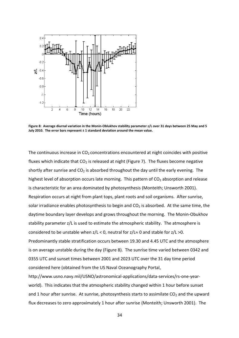
34

Figure 8: Average diurnal variation in the Monin-Oblukhov stability parameter z/L over 31 days between 25 May and 5 July 2010. The error bars represent ± 1 standard deviation around the mean value.

The continuous increase in CO2 concentrations encountered at night coincides with positive

fluxes which indicate that CO2 is released at night (Figure 7). The fluxes become negative

shortly after sunrise and CO2 is absorbed throughout the day until the early evening. The

highest level of absorption occurs late morning. This pattern of CO2 absorption and release

is characteristic for an area dominated by photosynthesis (Monteith; Unsworth 2001).

Respiration occurs at night from plant tops, plant roots and soil organisms. After sunrise,

solar irradiance enables photosynthesis to begin and CO2 is absorbed. At the same time, the

daytime boundary layer develops and grows throughout the morning. The Monin-Obukhov

stability parameter z/L is used to estimate the atmospheric stability. The atmosphere is

considered to be unstable when z/L < 0, neutral for z/L 0 and stable for z/L >0.

Predominantly stable stratification occurs between 19.30 and 4.45 UTC and the atmosphere

is on average unstable during the day (Figure 8). The sunrise time varied between 0342 and

0355 UTC and sunset times between 2001 and 2023 UTC over the 31 day time period

considered here (obtained from the US Naval Oceanography Portal,

http://www.usno.navy.mil/USNO/astronomical-applications/data-services/rs-one-year-

world). This indicates that the atmospheric stability changed within 1 hour before sunset

and 1 hour after sunrise. At sunrise, photosynthesis starts to assimilate CO2 and the upward

flux decreases to zero approximately 1 hour after sunrise (Monteith; Unsworth 2001). The

35

reverse process takes place shortly before sunset. The unstable daytime conditions enable

a well-mixed layer to develop in the boundary layer and help to vertically spread any near-

surface gasses, including CO2, thereby reducing the near-surface concentrations. The

shallow boundary layer and stable conditions at night prevent the dispersion of CO2.

Photosynthesis and respiration together with atmospheric stability explain the observed

diurnal variations in CO2 concentrations and fluxes. It was not possible to separate the

relative importance of these contributing factors from the data available but a strong linear

correlation (R2= 0.9443, P <0.001) was found between the mean flux and mean z/L over 31

days (figure not shown). The time when the CO2 flux changes from positive to negative, and

vice versa, corresponds to the time when the Monin-Obukhov parameter changes sign but

this also coincides with the expected time when a different phase of the photosynthetic

pathway becomes active. Annual measurements that include the winter period when

photosynthesis is limited would enable to separate the relative effect of boundary layer

height and photosynthesis.

The diurnal patterns in CO2 concentration derived from measurements at the Atmospheric

Observatory in Reading does not show a peak that could be associated with the morning

rush hour which is observed in other urban measurements. This indicates that nearby

traffic does not have a large effect on the CO2 concentrations at the measurement site. The

magnitude of the CO2 concentration will not be compared with other towns because

differences may be caused by regional and seasonal variations and differences in

measurement height. The largest difference was found when comparing CO2 fluxes with

those measured in other urban environments. Carbon dioxide fluxes in cities are generally

reported to remain positive throughout the day (for example, see Appendix 1). Our flux

measurements follow the same trend as the CO2 fluxes measured during the summer at the

University of Helsinki, which is surrounded by buildings and extensive vegetation (Jarvi et al.

2009). The origin of the discrepancy between CO2 fluxes in Reading and most other urban

centres may be elucidated by examining more closely where the [CO2] measured by the

sensor originates from.

Point measurements do not measure concentrations or fluxes immediately below the sensor

but reflect the surface upwind. The area that contains sources and sinks that influence the

instrument at a certain height is referred to as the footprint (Foken 2008) or source area

36

(Schmid 1994). The concept of source area enables us to estimate the spatial scale of point

measurements. The source area is upwind from the sensor but its size and position are

constantly changing and depend on the wind velocity and direction, surface roughness and

atmospheric stability. Several models are available (Foken 2008) based on turbulent

diffusion in a Eulerian frame of reference or based on Lagrangian trajectory dispersion

models. Most models are derived assuming certain conditions, such as for use in forests or

during neutral stratification. The model SAM-2 developed by Schmid (1994) is based on

diffusion and was used in this work to estimate the source area of CO2 concentrations. The

footprint function used in the model describes the source area in terms of its special extent

and concentration distribution. The model assumes a flat surface with no obstacles that can

disturb the wind flow. It does not take changes in surface cover, i.e. roughness, into account.

The results are therefore only an approximation of the source area. The model requires the

input of the measurement height z (3 m), the roughness length z0 (0.06 m), the friction

velocity u*, the Obukhov length L and the standard deviation of the lateral wind fluctuations

v. The source area is aligned with the wind direction and elongated. The effect of

atmospheric stability on the source area is demonstrated for the 31st of May 2010 when

average wind speeds up to 5 m s-1 were recorded from a predominantly north-westerly

direction (Figure 9). Under weakly unstable (z/L= -0.123) conditions, the main source of CO2

is within 8 to 42 m from the sensor with the maximum at 25 m (Figure 10a), i.e. mostly

within the enclosure of the observation site. The total source area extended to 467 m in

length and only covered an area of 0.095 km2 over vegetation and open water (Figure 9b).

Under weakly stable conditions (z/L= 0.107), the main source area was narrow and

elongated up to 108 m away over vegetation (Figure 9a), with the maximum at 48 m, while

the total source area extended to 1670 m (Figure 9b) and covered an area of 0.643 km2.

Increasing the stability increases the source area while increasing the instability decreases

the source area (Figure 10). Turbulence in an unstable atmosphere promotes vertical

transport and limits horizontal transport. Under stable conditions, vertical transport is low

and the vertical wind profile increases more rapidly with height leading to more dominant

horizontal transport and thus a larger source area. The area immediately underneath the

sensor did not contribute under any conditions. The low measurement height (3 m) explains

why only localised effects were measured which are dominated by the extensive

surrounding vegetation on the university campus and is not representative of a typical urban

37

Figure 9: Estimated source area for CO2 measurements at the University of Reading based on Schmid’s model (1994) for

stable (z/L= 0.107, u*= 0.225 m s-1

, v=0.694 m s-1

) and unstable (z/L= -0.123, u*= 0.337 m s-1

, v= 1.24 m s-1

) conditions on the 31

st of May 2010 with a north-westerly wind direction. (a) The environment surrounding the sensor consits of

vegetation (green) and a few buildings (pink). The solid eliptic lines indicate the area with the maximum contribution to measured [CO2] in unstable (red) and stable (black) conditions. This corresponds to 10% of the relative effect level. The dashed lines indicate the total source area (100% relative effect level) in unstable (red) and stable (black) conditions. (b) Full extend of the total source areas as indicated in (a). (Map Source= Digimap/ Ordnance Survey).

NW wind

(a)

NW wind

(b)

Sensor

Sensor

0 m 700 m

0 m 100 m

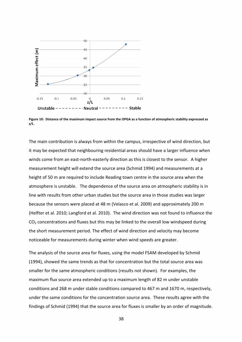
38

Figure 10: Distance of the maximum impact source from the OPGA as a function of atmospheric stability expressed as z/L.

The main contribution is always from within the campus, irrespective of wind direction, but

it may be expected that neighbouring residential areas should have a larger influence when

winds come from an east-north-easterly direction as this is closest to the sensor. A higher

measurement height will extend the source area (Schmid 1994) and measurements at a

height of 50 m are required to include Reading town centre in the source area when the

atmosphere is unstable. The dependence of the source area on atmospheric stability is in

line with results from other urban studies but the source area in those studies was larger

because the sensors were placed at 48 m (Velasco et al. 2009) and approximately 200 m

(Helfter et al. 2010; Langford et al. 2010). The wind direction was not found to influence the

CO2 concentrations and fluxes but this may be linked to the overall low windspeed during

the short measurement period. The effect of wind direction and velocity may become

noticeable for measurements during winter when wind speeds are greater.

The analysis of the source area for fluxes, using the model FSAM developed by Schmid

(1994), showed the same trends as that for concentration but the total source area was

smaller for the same atmospheric conditions (results not shown). For examples, the

maximum flux source area extended up to a maximum length of 82 m under unstable

conditions and 268 m under stable conditions compared to 467 m and 1670 m, respectively,

under the same conditions for the concentration source area. These results agree with the

findings of Schmid (1994) that the source area for fluxes is smaller by an order of magnitude.

39

The small flux source area indicates that the measured fluxes originate mainly from the

vegetated area immediately surrounding the measurement site with little influence from

nearby buildings or roads. This explains why the observed CO2 fluxes are representative of

the exchange over a vegetated area and not of that over an urban area.

4.3 Water vapour

4.3.1 Comparison of absolute humidity measurements

The open gas analyser measures the density of water vapour (mmol/m3) in the optical path

based on the amount of infra-red radiation absorbed by the water molecules in the beam.

The absolute humidity is the total mass of water vapour per unit volume of air (g/m3) and is

derived from this measurement by taking account of the molecular weight of water (1 mol

water = 18 g). Many methods are in use to measure the absolute humidity but the most

widely used is the psychrometric method (WMO 2008) and the absolute humidity estimated

from the open-path gas analyser will be compared here to this method. The psychrometric

method is based on the continuous measurements of the wet and dry bulb temperatures at

the Atmospheric Observatory, approximately 5 metres to the west of the open-path gas

analyser. Both temperatures are measured next to each other in a Large Stevenson Screen

with platinum resistance thermometers but the wet bulb thermometer is wrapped in a

cotton sleeve kept wet by capillary flow from a deionised water bath. Water evaporating

from the sleeve lowers the temperature and the amount of evaporation, and thus the

temperature depression, is proportional to the air humidity. The absolute humidity AH is

derived by the automated system (METFiDAS) from the following equations:

)273(5.461

1001000

dryT

eAH (3)

where e is the vapour pressure (hPa) and Tdry is the dry bulb temperature (°C). The vapour

pressure in turn is derived from the dry and wet bulb (Twet) temperatures using the semi-

empirical Regnault’s equation:

)(8.0 wetdrys TTee (4)

where 0.8 is the psychrometric coefficient and es is the saturated vapour pressure (hPa) with

respect to Twet and is derived from the empirical Teten’s equation

40

'exp

TT

TAee

w

wetos ( 5)

where e0 = 6.122 hPa and is the reference saturation pressure at 0°C, A = 17.67 and T’=

243.5. The accuracy of the absolute humidity derived from equations 9 – 11 depends on

several factors. The psychrometric coefficient used is an empirical value determined for a

screen psychrometer and is here assumed to be constant although in reality it varies with air

temperature and humidity and, in particular, it does vary markedly for ventilation rates

below 3-5 m s-1 (WMO 2008). It is recommended that screen psychrometers are artificially

aspirated to keep the ventilation rate constant. The effect of atmospheric pressure on the

vapour pressure is not taken into account and A should in fact be multiplied by p/1000

where p is the atmospheric pressure in hPa (WMO 2008). The accuracy further depends on

the accuracy of the thermometers, the use of appropriate coefficients and the use of clean

water and a clean sleeve to measure Twet , which can affect the vapour pressure of the water.

The assumption that adequate ventilation occurs in the screen is not always met at low wind

speeds, which dominated over most of the measurement period and particularly at night

(Figure 4).

The absolute humidity measured with the gas analyser (AHG) was compared with data

derived from the psychrometric method (AHT) over 21 days when no rain occurred. The

two datasets showed a strong linear correlation (R2 = 0.9932) and the values were similar

indicated by a slope of 0.962 (standard error = 0.00377) with an intercept of 0.00356

(standard error = 0.0351) when x = AHG (figure not shown). The standard error on the

intercept does not indicate a significant difference but the standard error on the slope is

considerably smaller than the slope value and indicates that the two data sets are

significantly different. This relationship shows that AHT is approximately 0.96 times AHG.

This is confirmed by visually examining the daily humidity differences which confirm that the

observed AHG is generally slightly greater than AHT (Figure 11) but follow the same trends.

The sources of uncertainty described earlier associated with both types of measurement can

all contribute to the small differences observed between the two data sets. The

measurement error on the absolute humidity measured with the open-path gas analyser

was determined to be 1.3% (see Error! Reference source not found.). The uncertainty on the

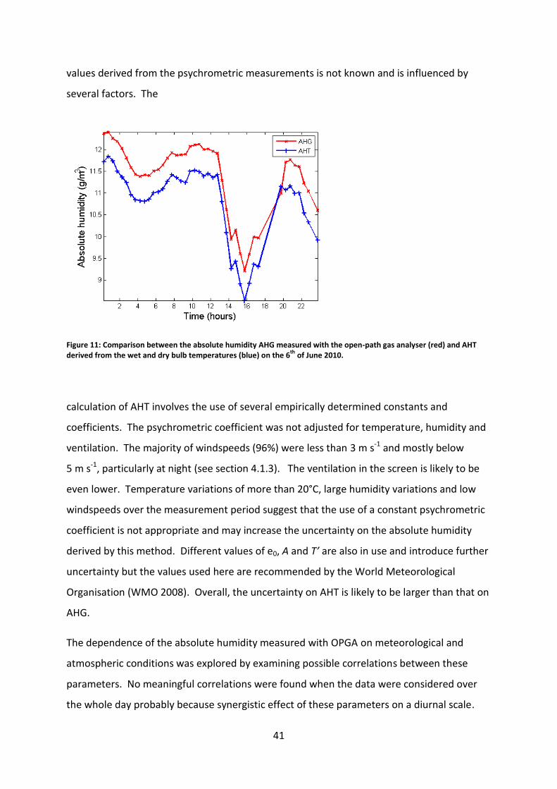
41

values derived from the psychrometric measurements is not known and is influenced by

several factors. The

Figure 11: Comparison between the absolute humidity AHG measured with the open-path gas analyser (red) and AHT derived from the wet and dry bulb temperatures (blue) on the 6

th of June 2010.

calculation of AHT involves the use of several empirically determined constants and

coefficients. The psychrometric coefficient was not adjusted for temperature, humidity and

ventilation. The majority of windspeeds (96%) were less than 3 m s-1 and mostly below

5 m s-1, particularly at night (see section 4.1.3). The ventilation in the screen is likely to be

even lower. Temperature variations of more than 20°C, large humidity variations and low

windspeeds over the measurement period suggest that the use of a constant psychrometric

coefficient is not appropriate and may increase the uncertainty on the absolute humidity

derived by this method. Different values of e0, A and T’ are also in use and introduce further

uncertainty but the values used here are recommended by the World Meteorological

Organisation (WMO 2008). Overall, the uncertainty on AHT is likely to be larger than that on

AHG.

The dependence of the absolute humidity measured with OPGA on meteorological and

atmospheric conditions was explored by examining possible correlations between these

parameters. No meaningful correlations were found when the data were considered over

the whole day probably because synergistic effect of these parameters on a diurnal scale.

42

For example, cooler temperatures at night coincide with low wind speeds and a stable

atmosphere; it not possible to identify the effect of temperature alone. To limit the effect of

this interdependence, correlations around midday alone were investigated when

atmospheric variability is less than on a diurnal scale. The absolute humidity measured

between 1000 and 1400 UTC over 29 days with the OPGA correlates with air temperatures

(R2 = 0.6013, P < 0.001) and shows a negative trend with net radiation Rn (R2 = -0.3518,

P <0.001). Air humidity can increase as the saturated vapour pressure increases with

temperature, according to the Clausius Clapeyron equation, but high levels of radiation may

cause excessive surface heating and activate protective physiological plant mechanisms to

prevent evaporation.

4.3.2 Latent heat fluxes

4.3.2.1 Evaporation

To facilitate comparison of data in this section, evaporation is expressed as latent heat flux

obtained from evaporation measurements according to equation 2 and from water vapour

fluxes derived from the eddy correlation method using equation 1. Evaporation

measurements are based on one daily observation at 0900 UTC when the evaporation over

the previous 24 hours is recorded. The latent heat fluxes measured throughout the day by

the OPGA system were integrated over the same time period to determine the evaporation

during the same 24 hours. No correlation was found between the latent heat flux from the

open-pan or Piche tube and that from the gas analyser (Figure 12).

Figure 12: Comparison between the latent heat derived from open-pan and Piche tube evaporation with that derived from the open-path gas analyser using the eddy correlation method. The linear regression line for each dataset is drawn on the graph and the linear regression equations, together with the correlation coefficient R

2, are listed. A blue line or

box refers to correlations with the Piche tube and red refers to correlations with the Open-pan.

43

Moreover, the results from the open-pan and Piche tube were only weakly correlated with

one another (R2 = 0.3203) (figure not shown). Although both measure evaporation from a

water source, evaporation is generally higher from the Piche tube (Figure 12). The World

Meteorological Organisation (WMO 2008) recommends evaporation measurements should

have a 95% confidence interval of ± 0.1 mm but concedes that in practice 1 mm is more

achievable. Based on the graduation of the measurement devises, the uncertainty on

reading water levels on the observation site at the University of Reading is ± 0.5 mm for the

Piche tubes and 0.01 mm for the open pan. This results in an uncertainty of ± 14.3 W m-2

and ± 5 W m-2 on a latent heat flux of 100 W m-2 for the Piche tube and open pan,

respectively. Accounting for the uncertainty in reading the water level does not change the

overall correlation but does reduce the magnitude of the difference between the two

methods. The difference is not likely to be related to the under-compensation for

precipitation events in the open-pan as rain only occurred on a few days (Figure 13). More

than 1 mm of rain only occurred on 6 days during the measuring period. In the Piche tube,

evaporation of deionised water does not occur directly from a water surface but from

wetted absorbent paper. Evaporation of water in the open-pan from a large water surface,

Figure 13: Latent heat estimated from the open-path gas analyser, open-pan evaporation and Piche tube evaporation between May and July 2010. The vertical black lines indicate days with minimum 0.5 mm rain.

44

although contaminated, may require more energy to overcome the surface tension of the

water compared to evaporation of water from wetted absorbent paper. The direct

radiation, wind and turbulence experienced by the open pan may still not be sufficient to

provide the additional energy.

Latent heat flux measured with the gas analyser is on average 8 times smaller than that

derived from the Piche tube and 7 times smaller than the open-pan (Figure 13). In these

methods, evaporation is not restricted by water availability while latent heat fluxes

measured by the gas analyser originate from many sources most of which are restricted by

water availability, mobility and plant physiology (see 2.2). The open-pan and Piche tube only

indicate how evaporation from a limited and specific water surface is affected by

meteorological conditions while the eddy correlation method indicates the evaporation from

the total complex environment. A direct comparison between the two types of

measurement is therefore of limited value as they are physically different measurements.

As discussed in section 4.2, the source area detected by the gas sensor is dominated by

vegetated soil with the main source derived from a grassy area. Water availability is

expected to be high after precipitation but no trend was found between latent heat flux and

precipitation or time since the last precipitation occurred (Figure 13). Infrequent and low

levels of precipitation, often less than 1 mm for less than 30 minutes, leading to depletion of

soil moisture may account for high levels of moisture absorption after precipitation and low

evaporation.

No significant correlations were found between the latent heat flux derived from the gas

analyser and wind speed, wind direction or humidity. The correlation (R2 = 0.5146) between

temperature and latent heat flux was driven by the simultaneous diurnal variation of both

variables but did not relate to the temperature between 1000 and 1400 UTC (R2 = 0.1889).

Daytime maximum temperatures alone do not determine the magnitude of the latent heat

flux. Multiple regression between the available meteorological parameters and latent heat

flux was not able to produce a satisfactory model. These results indicate that latent heat

fluxes are driven by a complex interaction of multiple parameters and not only by

45

meteorological conditions; any model should include parameters representing the condition

of the surface.

4.3.2.2 Potential evaporation

Latent heat fluxes (E1) were derived from meteorological observations according to the

Penman-Monteith equation (equation 5). These were used together with net radiation (Rn)

and ground flux (G) measurements to estimate the sensible heat flux (H1) derived from the

energy balance where Rn = E1 + H1 + G. Latent heat (E2), discussed in the previous section,

and sensible heat (H2) fluxes were also obtained from the measurement system associated

with the OPGA based on the eddy correlation method.

Figure 14: Comparison of the latent heat fluxes estimated from the open-path gas analyser (E2) and the Penman-

Monteith (PM) equation (E1) over 18 days between the 25th

of May and the 11th

of July 2010. The black limits indicate the 95% confidence interval as an indication of the spread of the data at a time point over a period of 18 days.

Both datasets show that latent heat fluxes are positive during the day and close to zero at

night but they vary greatly in their magnitude with maximum daytime latent heat fluxes E1

approximately 7 times larger than E2 (Figure 14). Consequently, large differences are also

seen in the sensible heat fluxes (Figure 15 and Figure 16). A mean midday Bowen ratio (β=

H/E) of 0.26 when using the Penman-Monteith equation, confirms that this estimate

assumes low moisture restrictions and is typical for well-irrigated crops and grassland

(Wilson et al. 2002b) . In contrast, a mean maximum Bowen ratio of 4.9 was derived from

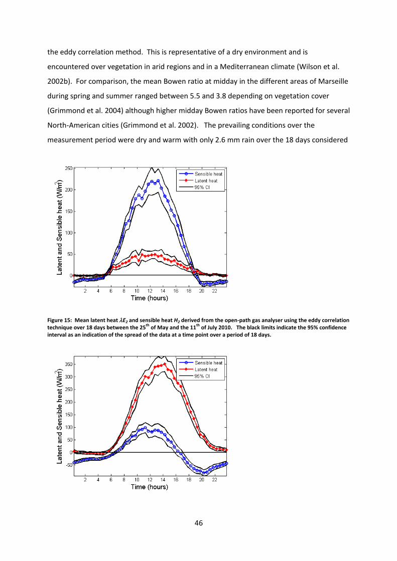
46

the eddy correlation method. This is representative of a dry environment and is

encountered over vegetation in arid regions and in a Mediterranean climate (Wilson et al.

2002b). For comparison, the mean Bowen ratio at midday in the different areas of Marseille

during spring and summer ranged between 5.5 and 3.8 depending on vegetation cover

(Grimmond et al. 2004) although higher midday Bowen ratios have been reported for several

North-American cities (Grimmond et al. 2002). The prevailing conditions over the

measurement period were dry and warm with only 2.6 mm rain over the 18 days considered

Figure 15: Mean latent heat E2 and sensible heat H2 derived from the open-path gas analyser using the eddy correlation technique over 18 days between the 25

th of May and the 11

th of July 2010. The black limits indicate the 95% confidence

interval as an indication of the spread of the data at a time point over a period of 18 days.

47

Figure 16: Mean latent heat E1, derived from the Penman-Monteith method, and sensible heat H1 estimated from the energy budget, averaged over 18 days between the 25

th of May and the 11

th of July 2010. The black limits indicate the

95% confidence interval as an indication of the spread of the data at a time point over a period of 18 days.

here and similarly low rainfall on intervening days. Although not identical to a

Mediterranean climate, the vegetation is less adapted to drought and heat and may respond

more quickly to these conditions. This was confirmed by the grass turning yellow over the

measurement period. Dry soil limits direct evaporation while plant stress, caused by lack of

water and high daytime temperatures, also restricts stomatal evaporation. The main source

area for the fluxes consists predominantly of grass-covered soil. Grassland is more sensitive

to soil moisture than trees because its shallow roots cannot access deep ground water

(Wilson et al. 2002b). This suggests that arid vegetation has not dissimilar surface properties

as impervious urban surfaces.

The surface resistance rs was assumed to be constant at 60 s m-1 for the calculation of E1. In

reality, rs depends on water availability and varies throughout the day as the stomatal

resistance changes. Seasonal differences associated with leaf area can be ignored here as all

the measurements were taken in late spring and early summer. An rs value of 60 s m-1 is

representative of midday conditions over well-irrigated crops but values of several hundred

s m-1 are found over other types of vegetation and 563 s m-1 was found over grassland under

very dry conditions (Wilson et al. 2002b). Increasing the surface resistance rs to 200 s m-1 to

represent dry conditions, although this may still be an underestimation, reduced the mean

midday latent heat flux by 29.5% (Table 7). This also includes the effect of changing the

measurement height z, used to calculate the aerodynamic resistance (Equation 3), to 3 m

which is the height at which the wind speed is measured. Originally, E1 assumed a

measurement height of 1.5 m and corresponds to the height of the temperature

measurement. The effect of changing z alone was small compared to the other effects (data

not shown). The estimate of ra was based on a roughness length z0 of 0.01 m to estimate E1

and applies to an open, level surface with short grass. However, the measurement

environment also contained long grass, shrubs, trees and buildings and a roughness length

of 0.06 m was used together with rs of 200 s m -1 and a measurement height of 3 m to

explore the uncertainty on ra. Using these assumptions, the latent heat flux decreased by

37.0% and increased the Bowen ratio from 0.26 to 1.1 (Table 7). This analysis indicates that

48

the surface resistance introduces more uncertainty on the latent heat flux calculations than

the aerodynamic resistance. The latent heat flux decreases logarithmically as rs and ra

increase and is particularly sensitive to changes in values within the range of interest for the

Table 7: Impact of changing the surface resistance rs, measurement height z and roughness length z0 on the mean midday latent heat flux derived from the Penman-Monteith equation and on the Bowen ratio. Midday refers to the period between 1000 and 1400 UTC. The standard deviation gives an indication of the spread of latent heat fluxes over the measurement period and does not represent intrinsic measurement uncertainties.

Mean Midday

Latent heat flux

(W m-2)

Standard deviation

(W m-2)

Difference in latent

heat flux

(%)

Bowen ratio

E1: rs = 60 s m-1,

z = 1.5 m, z0 = 0.01 m

319 88.4 0.26

rs = 200 s m-1, z = 3 m,

z0 = 0.01 m

225 67.4 29.5 0.80

rs = 200 s m-1, z = 3 m,

z0 = 0.06 m

201 60.1 37.0 1.1

conditions applicable to the measurement site in Reading (Sinclair 2004). Moreover,

atmospheric stability was not taken into account when calculating ra and neutral stability

was assumed. We can conclude that a high level of uncertainty is associated with the

Penman-Monteith assumptions and the method used with constant parameters is not an

appropriate reference method. The modified values are still different by a factor of 4

compared to those derived from the OPGA system, although the parameters may still not

have been optimum, but it does suggest that other aspects apart from aerodynamic and

surface resistances as well as measurement uncertainty play a role.

The sensible heat H1 became negative around 1630 UTC, compared to 1945 UTC for H2, and

reached values as low as -80 W m-1 by 2000UTC ( Figure 15 and Figure 16). These values

appear highly questionable in a warm, dry season when sunset occurred as late as 2025 UTC

and, assuming all the measurements are correct, gives further indication that a high level of

uncertainty is associated with the latent heat flux derived from the Penman-Monteith

equation.

49

The estimation of H1 is based on the assumption of energy balance closure while the

measurements of H2 and E2 make no such assumptions. Accounting for a mean midday

ground flux of 46 W m-2, based on ground flux measurements (data not shown), a lack of

energy balance closure at midday of approximately 20% was found. This agrees with an

average energy imbalance in the order of 20% over vegetation obtained from a FLUXNET

study of 22 sites (Wilson et al. 2002a). In that study, the closure improved with increased

turbulence and a lack of closure of the energy balance was attributed to underestimating

turbulence. Foken (2008b) also suggests that the imbalance is not due to measurement

errors in the eddy correlation method or radiation measurements but attributes the lack of

closure to the omission of large scale eddies which have a significant contribution to the

energy exchange. This implies that longer block averaging periods should be considered. To

test this hypothesis, the measurements were re-analysed by averaging over 60 minutes and

these results were compared with the original data averaged over 30 minutes and

subsequently averaged over 1 hour, as described by Langford et al. (2010). Eddies with a

time period between 30 and 60 minutes increase the latent heat flux by 1.2% (Figure 17).

Figure 17: Comparison of latent heat derived from the OPGA averaged over 30 min and 1 hour. The data were obtained on 18 days between the 25

th of May and the 11

th of July 2010. The analysis was based on 432 data points.

This compares to a 1% discrepancy found by Helfter et al. (2010) when the average time was

extended from 30 min to 2 hours for sensible heat fluxes in London measured at a height of

200 m. Langford et al. (2010) found sensible heat flux losses of 3.1% for a 25 min averaging

50

time compared to 60 min at the same site in London. Our results imply that hardly any large

scale turbulences have been filtered out by choosing a 30 min averaging period. Increasing

the averaging period further is unlikely to make up for the lack of energy balance closure

while increasing the risk of non-stationarity. In addition, the measurement uncertainty

associated with the OPGA instrument is very small (see 4.1) and cannot account for the lack

in energy closure. This leads to the hypothesis that the cumulative effect of different errors

related to data processing, as discussed in section 2.3.2, may be responsible for errors of up

to 20% and account for the lack of energy balance closure.

51

Chapter 5: Conclusions

The performance and stability of an open-path gas analyser that measures CO2 and water

vapour concentrations was examined over a 9 week period by measuring weekly known

amounts of gas and determining the calibration factors. The instrument’s values were stable

and the uncertainty due to the calibration only was less than 0.09% for CO2 and less than

0.6% for water vapour. This resulted in a measurement uncertainty of 0.3% on

concentrations of CO2 and 1.3% for water vapour. This random error is small compared to

the natural range of gas concentrations to be measured which makes the instrument

suitable for the measurement of [CO2] and water vapour. The main drawback of the OPGA is

that data collected during precipitation, dew or fog must be rejected. Droplets in the air in

the optical path or deposited on the windows lead to spurious data which have to be

removed. Installing the instrument at an angle away from the vertical direction and coating

with a hydrophobic wax did not prevent the deposition of droplets. Other substances, such

as pollen and dust, were not found to contaminate the window. The performance of the

instrument over 9 weeks suggests that weekly calibrations may not be necessary but further

work is required to determine the maximum acceptable calibration interval. The inability to

measure gasses accurately during precipitation and condensation events makes the OPGA

less suitable for continuous use in climates where these weather phenomena occur

frequently, such as in the UK, and the use of a protective shroud with the OPGA or a closed-

path gas analyser may be more appropriate.

Apart from errors associated with the gas analyser, other sources of uncertainty must be

taken into account when the OPGA is used together with a sonic anemometer to estimate

fluxes of latent heat, sensible heat and CO2 using the eddy correlation method. Additional

errors are associated with the instrument installation on the measurement site and the

extensive post-field data processing that is required. Data processing, including correction

procedures, introduces uncertainty and can lead to a bias in the results. There are no agreed

procedures and individual researchers decide how best to handle their data. Many

discussions are ongoing on the validity of certain corrections or the best methods to employ.

An additional complicating factor is that the appropriate corrections are not generally

applicable but depend on the prevailing atmospheric conditions. One of the major sources

of uncertainty is related to flux measurements under low turbulent conditions, which occur

52

mainly during the night, and the choice of an acceptable u* threshold. This can lead to an

underestimation of CO2 respiration and has important consequences for the carbon budget.

The majority of the flux measurements and the discussions around data processing relate to

measurements over vegetation. These techniques have been adopted for urban

measurements but this area of research is still under-represented. It has not been possible

to define the overall magnitude of the uncertainty associated with flux measurements due

to the multitude of sources of error and their unknown synergistic effects but the possibility

of large errors must be considered when interpreting data.

Clear diurnal variations in CO2 concentrations and fluxes were observed with high

concentrations at night dropping sharply after sunrise to reach a minimum in the late

afternoon. This diurnal pattern correlated with positive fluxes at night combined with stable

atmospheric conditions and with negative fluxes and unstable conditions during the day.

These results are characteristic for a vegetated area and not for an urban environment. An

analysis of the source area of gas concentrations confirmed that the main source of the CO2

concentration measured by the instrument at a height of 3 m is within less than 110 m from

the sensor and extends mainly over vegetation in most directions. The source area for fluxes

was smaller by an order of magnitude and is even more strongly dominated by vegetation.

The size of the source area varies with smaller source areas contributing under unstable

atmospheric conditions than under stable stratification. The diurnal pattern in CO2

concentration and fluxes can therefore be attributed to the change in boundary layer depth,

which is related to the atmospheric conditions, combined with the effect of photosynthesis

and respiration over vegetation. These results suggest that extensive green spaces in an

urban environment have an important role to play in the overall carbon exchange of a city.

The absolute humidity derived from the psychrometric method was, on average, 0.96 times

that measured with the OPGA. The small discrepancy between the two measurements may

be related to instrument error and the constants used to derive the absolute humidity from

the wet and dry bulb measurements. Particularly, lack of sufficient ventilation in the screen

at low windspeeds and the use of a constant value for the psychrometer coefficient may be

inappropriate as this should be adjusted according to wind speed, temperature and

humidity.

53

Several methods can be used to estimate the latent heat flux but comparative studies are

difficult to find presumably because each method is based on widely different principles and

represent different aspects of latent heat flux in the environment. The comparison of the

latent heat flux derived from the eddy correlation technique and open pan, Piche tube and

Penman-Monteith evaporation identified that the latent heat flux from the eddy correlation

method is on average 4 to 8 times lower than that measured with the other methods. The

open pan and Piche tube indicate evaporation from an unrestricted, open water surface and

represent how evaporation from a specific water surface is affected by meteorological

conditions while the eddy correlation method indicates the evaporation from the total

complex environment. The Penman-Monteith method assumes a saturated surface and

measures potential and not actual evaporation. Comparison between these methods and

latent heat fluxes measured over vegetation during warm and dry conditions are bound to

show large discrepancies as the physical principals and assumptions of the measurements

differ. In addition, each of the measurements has considerable sources of uncertainties

associated with them related to measurement uncertainty, the parameters used to derive

the results, assumptions made about atmospheric stability and using constants where in

reality the values depend on the atmospheric conditions. The source area of the latent heat

flux derived from the eddy correlation method consists of vegetation, mainly grass with

some trees, where evaporation is restricted by moisture availability, mobility and plant

physiology as well as atmospheric conditions. The warm and dry conditions during the

measurement period lead to a Bowen ratio similar to values measured over arid and

Mediterranean regions or some urban centres with little vegetation. Overall, the energy

fluxes derived from the eddy correlation method best represent the fluxes of the total

environment surrounding the sensor. For this method, errors up to 20% assumed to

originate from the data processing step, must be taken into account and lead to

underestimation of energy fluxes and a lack of energy balance closure.

Latent heat and CO2 fluxes from the vegetated source area are linked as plant physiology

plays an important role for both. The low latent heat fluxes indicate that plants were highly

stressed and this should also reduce the CO2 fluxes. Considering that the grass was yellow, it

is assumed that most of the CO2 fluxes originated from the trees. Measurements when the

54

soil is well watered would indicate the potential for CO2 exchange and the relative

contributions from grassland and trees.

The results from this work indicate that the atmospheric exchange over extensive green

areas within an urban environment is representative of the vegetated area only. This shows

the significance of parks in towns and the need to consider the intra-urban surface cover in

urban studies. It also highlights the importance of choosing an appropriate measurement

site and height when aiming to measure processes in a build environment. Conclusions from

this work are limited because several parameters that can affect the observations only

varied within narrow limits as the measurement period covered just a few weeks during late

spring and early summer. An extended measurement period including winter and summer is

required to derive more conclusions about the impact of atmospheric conditions and large

variations in photosynthesis, surface cover and characteristics.

Suggestions for future work

The results from this project have indicated that this research area would benefit from

further investigations to get a more comprehensive understanding of urban environments,

instrumentation and data processing. Areas of interest are:

Determine the maximum acceptable interval for user calibration of the OPGA.

Evaluate the suitability of an OPGA during periods of frequent rain and in freezing

temperatures, i.e. under prevailing winter conditions in the south of England.

Explore the potential of using a shroud to protect the OPGA from precipitation and

condensation.

Optimise and extend the post-field data handling process or evaluate available software.

Validate the code used for data processing by analysing a ‘Gold Standard’ dataset

obtainable from AmeriFlux (http://public.ornl.gov/ameriflux/gold-open_path.shtml).

Extend the measurement period to include all seasons to investigate :

- Annual variations in concentrations and fluxes.

- The relative impact of photosynthesis and boundary layer height on variations in

CO2 fluxes by including periods with strong and weak photosynthetic activity.

- Effect of windspeed and direction on the source areas, fluxes and concentrations

by including periods with higher windspeeds.

55

Detailed investigation of the impact of green spaces as well as dispersed vegetation

throughout a city on the overall urban climate and carbon budget by comparing

atmospheric conditions in parks with surrounding build-up areas. The minimum area of

parkland with respect to the size of the city, which is required to have a beneficial effect

on the urban climate, should be determined for different climatic conditions and types of

vegetation. This could potentially be a tool for urban designers to mitigate the urban

heat effect.

Appendix 1: CO2 concentration and fluxes in Mexico City and London

Figure 18: Comparison of the average diurnal pattern of CO2 concentrations and CO2 fluxes in three towns. (a) is [CO2] and (b) flux in Reading, as reported in Figures 6 and 7. The error bars represent ± 1 standard deviation. (c) is [CO2] and (d) fluxes in London ((Helfter et aI. 2010). The error bars in (c) represent ± 1 standard deviation. (e) is [CO2] and (f) fluxes in Mexico City (Velasco et al. 2009). The gray shadow represents ±1 standard deviation from the total 2006 average and gives and indication of the day-to-day variability. The timescale corresponds to the local standard time.

(a)

(b)

(c)

(d)

(e)

(f)

Time of day (hours)

Time of day (hours)

CO

2 f

lux

(µm

ol m

-2 s

-1)

C

O2

flu

x (µ

mo

l m-2

s-1

)

C

O2 c

on

cen

trat

ion

(p

pm

v)

C

O2 c

on

cen

tra

tio

n (

pp

mv)

C

O2 c

on

cen

tra

tio

n (

pp

mv)

References

Arnell, N., 2002: Hydrology and Global Environmental Change. Pearson Education Limited,

346 pp. Aubinet, M., and Coauthors, 2000: Estimates of the annual net carbon and water exchange

of forests: The EUROFLUX methodology. Advances in Ecological Research, Vol 30, Academic Press Inc, 113-175.

Baldocchi, D., and Coauthors, 2001: FLUXNET: A new tool to study the temporal and spatial variability of ecosystem-scale carbon dioxide, water vapor, and energy flux densities. Bulletin of the American Meteorological Society, 82, 2415-2434.

Baldocchi, D. D., 2003: Assessing the eddy covariance technique for evaluating carbon dioxide exchange rates of ecosystems: past, present and future. Global Change Biology, 9, 479-492.

Burba, G., and D. Anderson 2007: Introduction to the Eddy Covariance Method: General Guidelines and Conventional Workflow. Li-cor Biosciences.

Burba, G. G., D. K. McDermitt, A. Grelle, D. J. Anderson, and L. K. Xu, 2008: Addressing the influence of instrument surface heat exchange on the measurements of CO2 flux from open-path gas analyzers. Global Change Biology, 14, 1854-1876.

Burns, S. P., and Coauthors, 2009: An Evaluation of Calibration Techniques for In Situ Carbon Dioxide Measurements Using a Programmable Portable Trace-Gas Measuring System. Journal of Atmospheric and Oceanic Technology, 26, 291-316.

Clement, R. J., G. G. Burba, A. Grelle, D. J. Anderson, and J. B. Moncrieff, 2009: Improved trace gas flux estimation through IRGA sampling optimization. Agricultural and Forest Meteorology, 149, 623-638.

FAO, cited 2010: Crop evapotranspiration - Guidelines for computer crop water requirements. FAO Irrigation and drainage paper 56. [Available online at http://www.fao.org/docrep/x0490e/x0490e06.htm.]

Finnigan, J., 2008: An introduction to flux measurements in difficult conditions. Ecological Applications, 18, 1340-1350.

Finnigan, J. J., R. Clement, Y. Malhi, R. Leuning, and H. A. Cleugh, 2003: A re-evaluation of long-term flux measurement techniques - Part I: Averaging and coordinate rotation. Boundary-Layer Meteorology, 107, 1-48.

Foken, T., 2008: Micro-meteorology. Springer Verlag, 306 pp. George, K., L. H. Ziska, J. A. Bunce, and B. Quebedeaux, 2007: Elevated atmospheric CO2

concentration and temperature across an urban-rural transect. Atmospheric Environment, 41, 7654-7665.

Goring, D. G., and V. I. Nikora, 2002: Despiking acoustic Doppler velocimeter data. Journal of Hydraulic Engineering-Asce, 128, 117-126.

Grelle, A., and G. Burba, 2007: Fine-wire thermometer to correct CO2 fluxes by open-path analyzers for artificial density fluctuations. Agricultural and Forest Meteorology, 147, 48-57.

Grimmond, C. S. B., T. S. King, F. D. Cropley, D. J. Nowak, and C. Souch, 2002: Local-scale fluxes of carbon dioxide in urban environments: methodological challenges and results from Chicago. Environmental Pollution, 116, S243-S254.

58

Grimmond, C. S. B., J. A. Salmond, T. R. Oke, B. Offerle, and A. Lemonsu, 2004: Flux and turbulence measurements at a densely built-up site in Marseille: Heat, mass (water and carbon dioxide), and momentum. Journal of Geophysical Research-Atmospheres, 109, 19.

Gu, L. H., and Coauthors, 2005: Objective threshold determination for nighttime eddy flux filtering. Agricultural and Forest Meteorology, 128, 179-197.

Helfter, C., D. Famulari, G. J. Phillips, J. F. Barlow, and C. R. Wood, 2010: Controls of carbon dioxide concentrations and fluxes above central London. In prepartion for submission in Atmos Chem Phys.

Henninger, S., 2008: Analysis of near surface CO2 variability within the urban area of Essen, Germany. Meteorologische Zeitschrift, 17, 19-27.

Heusinkveld, B. G., A. F. G. Jacobs, and A. A. M. Holtslag, 2008: Effect of open-path gas analyzer wetness on eddy covariance flux measurements: A proposed solution. Agricultural and Forest Meteorology, 148, 1563-1573.

IPCC, 2007: IPCC Fourth Assesment Report (AR4) - The Physical Science Basis. Cambridge University Press, 996 pp.

Jarvi, L., and Coauthors, 2009: Comparison of net CO2 fluxes measured with open- and closed-path infrared gas analyzers in an urban complex environment. Boreal Environment Research, 14, 499-514.

Kaimal, J. C., and J. J. Finnigan, 1994: Atmospheric Boundary Layer Flows - Their structure and measurement. Oxford University Press, 289 pp.

Kiehl, J. T., and K. E. Trenberth, 1997: Earth's annual global mean energy budget. Bulletin of the American Meteorological Society, 78, 197-208.

Langford, B., and Coauthors, 2010: Fluxes and concentrations of volatile organic compounds above central London, UK. Atmospheric Chemistry and Physics, 10, 627-645.

Mahrt, L., 2010: Computing turbulent fluxes near the surface: Needed improvements. Agricultural and Forest Meteorology, 150, 501-509.

Matese, A., B. Gioli, F. P. Vaccari, A. Zaldei, and F. Miglietta, 2009: Carbon Dioxide Emissions of the City Center of Firenze, Italy: Measurement, Evaluation, and Source Partitioning. Journal of Applied Meteorology and Climatology, 48, 1940-1947.

Mauder, M., and Coauthors, 2007: The energy balance experiment EBEX-2000. Part II: Intercomparison of eddy-covariance sensors and post-field data processing methods. Boundary-Layer Meteorology, 123, 29-54.

Moffat, A. M., and Coauthors, 2007: Comprehensive comparison of gap-filling techniques for eddy covariance net carbon fluxes. Agricultural and Forest Meteorology, 147, 209-232.

Monteith, J. L., and M. Unsworth, 2001: Principles of Environmental Physics. Butterworth - Heinemann, 291 pp.

Nemitz, E., K. J. Hargreaves, A. G. McDonald, J. R. Dorsey, and D. Fowler, 2002: Meteorological measurements of the urban heat budget and CO2 emissions on a city scale. Environmental Science & Technology, 36, 3139-3146.

Newton, T., T. R. Oke, C. S. B. Grimmond, and M. Roth, 2007: The suburban energy balance in Miami, Florida. Geografiska Annaler Series a-Physical Geography, 89A, 331-347.

Offerle, B., C. S. B. Grimmond, K. Fortuniak, and W. Pawlak, 2006: Intraurban differences of surface energy fluxes in a central European city. Journal of Applied Meteorology and Climatology, 45, 125-136.

Oke, T. R., 1995: Boundary Layer Climates. Routledge, 435 pp.

59

Richardson, A. D., and Coauthors, 2006: A multi-site analysis of random error in tower-based measurements of carbon and energy fluxes. Agricultural and Forest Meteorology, 136, 1-18.

Rigby, M., R. Toumi, R. Fisher, D. Lowry, and E. G. Nisbet, 2008: First continuous measurements of CO2 mixing ratio in central London using a compact diffusion probe. Atmospheric Environment, 42, 8943-8953.

Schmid, H. P., 1994: Source areas for scalars and scalar fluxes. Boundary-Layer Meteorology, 67, 293-318.

Sinclair, V., 2004: Boundary Layer Influences on Pollution in Reading, Department of Meteorology, University of Reading, 48 pp

Thorsson, S., and I. Eliasson, 2003: An intra-urban thermal breeze in Goteborg, Sweden. Theoretical and Applied Climatology, 75, 93-104.

Velasco, E., and Coauthors, 2009: Eddy covariance flux measurements of pollutant gases in urban Mexico City. Atmospheric Chemistry and Physics, 9, 7325-7342.

Vickers, D., M. Gockede, and B. E. Law, 2010: Uncertainty estimates for 1-h averaged turbulence fluxes of carbon dioxide, latent heat and sensible heat. Tellus Series B-Chemical and Physical Meteorology, 62B, 87-99.

Webb, E. K., G. I. Pearman, and R. Leuning, 1980: Correction of flux measurements for density effects due to heat and wate vapour transfer. Quarterly Journal of the Royal Meteorological Society, 106, 85-100.

Wilczak, J. M., S. P. Oncley, and S. A. Stage, 2001: Sonic anemometer tilt correction algorithms. Boundary-Layer Meteorology, 99, 127-150.

Wilson, K., and Coauthors, 2002a: Energy balance closure at FLUXNET sites. Agricultural and Forest Meteorology, 113, 223-243.

Wilson, K. B., and Coauthors, 2002b: Energy partitioning between latent and sensible heat flux during the warm season at FLUXNET sites. Water Resources Research, 38.

WMO, 2008: WMO Guide to Meteorological Instruments and Methods of Observation - Part I: Measurements of meteorological measurements. Seventh Edition ed., 369 pp.