uncertainties in global crop model frameworks: effects of ...pure.iiasa.ac.at/14232/1/uncertainties...

1

Uncertainties in global crop model frameworks: effects of

cultivar distribution, crop management and soil handling on

crop yield estimates

Christian Folberth1, Joshua Elliott2,3, Christoph Müller4, Juraj Balkovič1,5, James 5

Chryssanthacopoulos3, Roberto C. Izaurralde6,7, Curtis D. Jones6, Nikolay Khabarov1,

Wenfeng Liu8, Ashwan Reddy6, Erwin Schmid9, Rastislav Skalský1,10, Hong Yang8,11, Almut

Arneth12, Philippe Ciais13, Delphine Deryng3, Peter J. Lawrence14, Stefan Olin15, Thomas

A.M. Pugh12,16, Alex C. Ruane3,17, Xuhui Wang13,18

10

1International Institute for Applied Systems Analysis, Ecosystem Services and Management Program, 2361

Laxenburg, Austria

2University of Chicago and ANL Computation Institute, Chicago, IL 60637, USA

3Columbia University Center for Climate Systems Research and NASA Goddard Institute for Space Studies,

New York, NY 10025, USA 15

4Potsdam Institute for Climate Impact Research, 14473 Potsdam, Germany

5Comenius University in Bratislava, Department of Soil Science, 842 15 Bratislava, Slovak Republic

6University of Maryland, Department of Geographical Sciences, College Park, MD 20742, USA

7Texas A&M University, Texas AgriLife Research and Extension, Temple, TX 76502, USA

8Eawag, Swiss Federal Institute of Aquatic Science and Technology, CH-8600 Duebendorf, Switzerland 20

9University of Natural Resources and Life Sciences, Institute for Sustainable Economic Development, 1180

Vienna, Austria

10Soil Science and Conservation Research Institute, National Agricultural and Food Centre, 82713 Bratis lava,

Slovak Republic

11Department of Environmental Sciences, University of Basel, Petersplatz 1, CH-4003 Basel, Switzerland 25

12Karlsruhe Institute of Technology, IMK-IFU, 82467 Garmisch-Partenkirchen, Germany

13Laboratoire des Sciences du Climat et de l’Environnement. CEA CNRS UVSQ Orme des Merisiers, F-

91191 Gif-sur-Yvette, France

14National Center for Atmospheric Research, Earth System Laboratory, Boulder, CO 80307, USA

15Department of Physical Geography and Ecosystem Science, Lund University, 223 62 Lund, Sweden 30

16School of Geography, Earth & Environmental Science and Birmingham Institute of Forest Research,

University of Birmingham, Edgbaston, Birmingham, B15 2TT, United Kingdom

17National Aeronautics and Space Administration Goddard Institute for Space Studies, New York, NY 10025,

USA

18Peking University, Sino-French Institute of Earth System Sciences, 100871 Beijing, China 35

Correspondence to: Christian Folberth ([email protected])

Biogeosciences Discuss., doi:10.5194/bg-2016-527, 2016Manuscript under review for journal BiogeosciencesPublished: 20 December 2016c© Author(s) 2016. CC-BY 3.0 License.

2

Abstract. Global gridded crop models (GGCMs) combine field-scale agronomic models or sets of plant growth

algorithms with gridded spatial input data to estimate spatially explicit crop yields and agricultural externalities 40

at the global scale. Differences in GGCM outputs arise from the use of different bio-physical models, setups,

and input data. While algorithms have been in the focus of recent GGCM comparisons, this study investigates

differences in maize and wheat yield estimates from five GGCMs based on the public domain field-scale model

Environmental Policy Integrated Climate (EPIC) that participate in the AgMIP Global Gridded Crop Model

Intercomparison (GGCMI) project. Albeit using the same crop model, the GGCMs differ in model version, 45

input data, management assumptions, parameterization, geographic distribution of cultivars, and selection of

subroutines e.g. for the estimation of potential evapotranspiration or soil erosion. The analyses reveal long-term

trends and inter-annual yield variability in the EPIC-based GGCMs to be highly sensitive to soil

parameterization and crop management. Absolute yield levels as well depend not only on nutrient supply but

also on the parameterization and distribution of crop cultivars. All GGCMs show an intermediate performance 50

in reproducing reported absolute yield levels or inter-annual dynamics. Our findings suggest that studies

focusing on the evaluation of differences in bio-physical routines may require further harmonization of input

data and management assumptions in order to eliminate background noise resulting from differences in model

setups. For agricultural impact assessments, employing a GGCM ensemble with its widely varying assumptions

in setups appears the best solution for bracketing such uncertainties as long as comprehensive global datasets 55

taking into account regional differences in crop management, cultivar distributions and coefficients for

parameterizing agro-environmental processes are lacking. Finally, we recommend improvements in the

documentation of setups and input data of GGCMs in order to allow for sound interpretability, comparability

and reproducibility of published results.

60

Keywords: agricultural management; agro-ecologic systems; evapotranspiration; soil data; global

agriculture

1 Introduction

Global gridded crop models (GGCMs) have become major tools in recent years for agricultural climate change

impact assessments (e.g. Liu et al., 2013; Balkovič et al., 2014; Elliott et al., 2014; Folberth et al., 2014; 65

Rosenzweig et al., 2014; Müller et al., 2015; Deryng et al., 2016) and water consumption studies (e.g. Liu et al.,

2007; Fader et al., 2010) among others. For some models, the global gridded version is a combination of (a) a

field-scale crop model, or collection of algorithms used to estimate yields and externalities of crop production

for a number of pixels covering a given region and (b) a model framework (MFW) that processes input data and

runs the model over large regions or the globe. The often high-complexity of these field-scale models is 70

contrasted by the scarcity of spatially detailed input data available for global-scale applications of GGCMs. This

requires assumptions on crop management and the use of agricultural inputs by modelers, which can differ

substantially among research groups. Fertilizer application rates may, for example, be (a) based on statistics

(Liu, 2009; Deryng et al., 2011; Folberth et al., 2012; Balkovič et al., 2014), (b) defined by contrasting

intensification systems (Skalský et al., 2008), or (c) integrated into management coefficients, e.g. if a model 75

does not contain explicit nutrient cycling routines (Fader et al., 2010). Other management related data such as

the handling of crop residues, fallow durations and tillage practices have yet to be compiled at the global scale.


3

Furthermore, the setup and parameterization of a GGCM depends on the evolving objectives used in its

development. The Environmental Policy Integrated Climate (EPIC) field-scale model, which is the focus of this

study, has been developed for assessing impacts of agricultural management on crop growth and externalities 80

like erosion rates and soil nutrient cycling (Williams et al., 1989). When it comes to long-term impacts of

climate change on agricultural production, however, soil erosion and nutrient depletion can affect yield

estimates over time due to nutrient deficits (Kuhn et al., 2010). To limit such effects and facilitate investigations

of climate impacts alone on plant growth, the model allows for annually resetting the soil profile. This in turn

eliminates interactions among crop management, soil and climate beyond the annual growing season, which can 85

be crucial for identifying effective adaptation options (Folberth et al., 2014; Folberth et al., 2016). In GGCM

studies, researchers may therefore opt for one setup over another depending on the object of investigation.

Besides different options of how to handle soils, the EPIC model provides six different methods for estimating

water erosion, five algorithms for estimating potential evapotranspiration (PET) as well as several subroutines

and suggested parameter ranges for nutrient cycling and gas diffusion within the soil (Gerik et al., 2014). 90

Hence, GGCMs, even of the same origin or model family, can exhibit substantial differences in simulated

outputs due to uncertainties originating from (a) field-scale models or modelled processes, (b) input data, and (c)

setup and parameterization. In order to systematically address uncertainties in GGCMs, the Inter-Sectoral

Impact Model Intercomparison Project (ISI-MIP; http://www.isi-mip.org; Warszawski et al., 2014) and the

Agricultural Model Intercomparison and Improvement (AgMIP) project (https://www.agmip.org; Rosenzweig et 95

al., 2013) compiled outputs from various GGCMs that had been forced with identical climate projections

(Hempel et al., 2013) in order to produce a joint agricultural climate change impact assessment (Rosenzweig et

al., 2014). These studies revealed that large differences remain among GGCMs even if they are based on

identical field-scale models. This emphasized the importance of distinguishing between biophysical plant

growth models that are used as a core of GGCMs on one hand and MFWs on the other. 100

For phase 1 of AgMIP’s Global Gridded Crop Modelling Intercomparison initiative (GGCMI;

http://www.agmip.org/ag-grid/ggcmi), several GGCMs have been forced with identical annual fertilizer

application rates, growing seasons and climate data to eliminate uncertainties resulting from these priority data

(Elliott et al., 2015). Among the 14 GGCMs participating in the study, five were based on the EPIC model,

namely EPIC-BOKU, EPIC-IIASA, EPIC-TAMU, GEPIC and PEPIC. The purpose of the present study is to 105

identify differences among these EPIC-based MFWs caused by input data, crop management and

parameterization. This allows for identifying priorities for further harmonization in the whole GGCM ensemble

in order to refine analyses of differences in biophysical algorithms globally. All MFWs were run for six crop

management intensities to evaluate the impact of nutrient and water supply on differences in crop yield

estimates. Here, we focus on maize in detail as a representative crop widely used in GGCM studies. 110

Complementary results are provided for wheat in Supplementary Information S4 as key findings were in close

agreement for both crops. In addition, various setup options were permutated for maize between two of the

GGCMs, EPIC-IIASA and GEPIC, to assess the contribution of certain setup aspects to deviations in yield

estimates. Outputs from an ensemble of non-EPIC-based GGCMs participating in phase 1 of the GGCMI

project that establishes both a general benchmark for global crop models, as well as the model-driven 115

uncertainty in GGCM simulations (Müller et al., 2016), are used as a reference to which to compare the EPIC-

based ensemble.


4

2 Methods and Data

2.1 The Environmental Policy Integrated Climate field scale model

The EPIC model was first developed in the 1980s to assess the impacts of soil management on crop yields 120

(Williams et al., 1989). It has been updated frequently to cover e.g. effects of elevated atmospheric CO2

concentration on plant growth (Stoeckle et al., 1992), detailed soil organic matter cycling (Izaurralde et al.,

2006, Izaurralde et al., 2012), and an extended number of crop types and cultivars (e.g. Kiniry et al., 1995;

Gaiser et al., 2010) among others (Gassman 2004).

EPIC estimates potential biomass increase on a daily time-step based on light interception and conversion of 125

CO2 to biomass. Plant growth and phenology are calculated based on the daily accumulation of heat units. Plant

growth is constrained by water and nutrient (nitrogen (N) and phosphorus (P)) deficits, adverse temperature, and

aeration stress. The potential biomass gain is subsequently adjusted by the major plant growth-regulating factor

on a given day to obtain the actual biomass increment. Root growth can be limited by soil strength, adverse soil

temperature, and aluminum toxicity. At maturity, the model calculates crop yield based on above ground 130

biomass and an actual harvest index HIa, which is estimated within a range given by potential HI (HImax) and

minimum HI under water stress (HImin). Besides plant growth and yield formation, EPIC estimates a wide range

of environmental externalities, for example wind and water erosion rates, turnover and partitioning of organic

carbon (OC), N and P, evapotranspiration (ET), fluxes of selected gases, and soil hydrologic processes.

2.2 EPIC model frameworks and complementary global gridded crop models included in the study 135

Different versions of the EPIC model have been implemented in the five EPIC-MFWs evaluated in the study:

EPIC-BOKU, EPIC-IIASA, GEPIC, and PEPIC use EPIC v.0810, while EPIC-TAMU uses the experimental

version v.1102. Main differences between the two structurally very similar model versions are outlined in

Supplementary S1.2, which also provides a comparison of maize yield estimates of the two model versions for

four selected sites. Besides different model versions, the selection of subroutines adds to differences in the set of 140

algorithms used for the simulations as well. E.g., EPIC allows for selecting from five estimation methods for

PET, namely Baier-Robertson, Priestly-Taylor, Penman, Penman-Monteith (PM), and Hargreaves (HG). Water

erosion can be estimated by one of eight methods, and there are 11 options for estimating or inputting the water

content at field capacity and wilting point. In addition, individual parameters and coefficients may be adjusted

by the user to adapt the model to local conditions (Gerik et al., 2014). 145

Table 1 provides an overview of major subroutines and parameters selected within the five EPIC-MFWs.

Another seven GGCMs (CLM-CROP, LPJ-GUESS, LPJmL, ORCHIDEE-crop, pAPSIM, pDSSAT, and

PEGASUS) contributing to GGCMI phase 1 were included to locate the EPIC ensemble within a wider

ensemble of GGCMs based on different sets of algorithms. They were selected based on the contribution of

outputs for at least two of three management setups: without nutrient limitation and default or fully harmonized 150

input data (fullharm; see Section 2.4) for maize or wheat. If only default or fullharm was supplied, the

corresponding other scenario was used as a substitute to keep the number of GGCMs across management

scenarios constant.

The following sub-sections provide key descriptions of the setups and rationales of the EPIC-based MFWs.

Information on input data and management scenarios are provided in Sect. 2.3-2.5. Additional information on all 155


5

GGCMs, including the seven non-EPIC-based GGCMs that were used for comparison with the EPIC-MFW

ensemble, are provided on the website of ISI-MIP (http://www.isimip.org) and in Müller et al. (2016).

2.2.1 EPIC-BOKU

EPIC-BOKU was initially developed to provide yield estimates at contrasting management intensities for land

use change and agro-economic models (Havlík et al. 2011, Schneider et al. 2011; Nelson et al., 2014; Frank et 160

al., 2015) at the European and global scales (Stolbovoy et al. 2007; Skalský et al., 2008; Elshout et al., 2015).

The spatial structure of its input data is based on a regular 5 arcmin grid, which is first aggregated to

homogenous response units (HRUs) based on a classification of physical characteristics (elevation, slope, soil).

The HRUs are subsequently intersected with administrative units (national borders at the global scale) that

determine specific crop management parameters, which are derived from databases or socio-economic data. The 165

field-scale model is run for each of the resulting simulation units (SimU). For comparison with GGCMs running

at a 0.5°x0.5° resolution, the results from the SimUs were resampled based on the pixel-weighted 5 arcmin

model outputs per 0.5°x0.5° grid. Presently, the GGCM runs two nutrient management intensities, high-input

and low-input agriculture with accordingly high or low fertilizer application rates. For the default simulations,

outputs from the high-input runs were submitted, corresponding to non-nutrient limited yield potential with 170

default growing season assumptions. Further management data such as growing seasons have been compiled

from various sources as specified in Skalský et al. (2008).

2.2.2 EPIC-IIASA

EPIC-IIASA has been developed in parallel to EPIC-BOKU, partly by the same researchers and shares the same

spatial data structure based on HRUs and SimUs. Parameterizations and input data have been adjusted 175

throughout research projects resulting in a substantially differing setup with the major remaining communality

being the use of a static soil profile (Table 1). Growing seasons have been adopted from Sacks et al. (2010) and

crop-specific spatially explicit N and P application rates from Mueller et al. (2012). Focus regions of recent

studies for which model setups have been adjusted are the EU (e.g. Balkovič et al., 2013) and China (Xiong et

al., 2014a; Xiong et al., 2014b) besides global applications (Balkovic et al. 2014 Xiong et al. 2016). 180

2.2.3 EPIC-TAMU

EPIC-TAMU follows the model development and implementation of EPIC, version 1102, which accounts for C

and N stocks and flows in managed terrestrial ecosystems (Izaurralde et al. 2012). As in EPIC v. 0810, the

coupled C and N model in EPIC-TAMU follows the conceptual pool structure of the Century model (Izaurralde

et al., 2006). Mineralization and immobilization of C and N also follows the approach in Century but a recent 185

option has been added to describe C and N of microbial biomass following the approach used in the Phoenix

model (McGill et al., 1981). The EPIC-TAMU version also contains algorithms to model the effects of biochar

additions on crop productivity, soil pH, and cation exchange capacity (Lychuk et al., 2015). Other developments

include a mechanistic model to describe microbial denitrification and the corresponding feedback on

decomposition (Izaurralde et al., 2012). 190

EPIC-TAMU has primarily been used for field-scale and regional-scale simulations (Gelfand et al., 2013; Zhang

et al., 2015). It has been adapted with minimal changes for use as part of the AgMIP GGCMI project, and has


6

otherwise not been previously used for global simulations. As a result, no default simulations (see Section 2.4)

were produced. To keep the number of EPIC-MFWs in evaluations across management scenarios constant, the

fully harmonized setup was also used as default. 195

2.2.4 GEPIC

The GEPIC MFW was originally developed for studies of global crop-water relations (Liu et al., 2007). In its

present version, it uses input data for planting dates, growing season length, P fertilizer application rates, and

cultivar distributions besides the original input data elevation, slope, country/region, N fertilizer application

rates, and irrigation water management (Folberth et al., 2012). Default fertilizer inputs are mainly based on the 200

FertiStat database (FAO, 2007) and have been extrapolated for maize based on the human development index

(HDI) for countries lacking data.

More recently, the MFW has been setup for applications in sub-Saharan Africa based on a regional calibration

(Gaiser et al., 2010) and thoroughly evaluated in various studies (e.g. Folberth et al., 2012; Folberth et al., 2014;

van der Velde et al., 2014). The authors found that when using dynamic soil profiles in the setup, the model 205

reproduces yields around the year 2000 well after a spin-up of 30 years (Folberth et al., 2012). Extending the

simulation period may result in erosion of the whole soil profile at some point or complete nutrient depletion in

grid cells that lack fertilizer inputs. To avoid resulting detrimental effects on crop yields and unrealistically long

monocultures, the model is run for each decade of the study period separately, which aims at mimicking fallow

rotation with an average cultivation period of 40 years and complete recovery of the soil profile afterwards (see 210

Figure S1-1).

2.2.5 PEPIC

PEPIC is a global EPIC-MFW developed at the Swiss Federal Institute of Aquatic Science and Technology

(Eawag) initially based on GEPIC, which had been developed at the same institute. Hence, the two MFWs have

similar features in software design and default input data. However, one of the main purposes of PEPIC was to 215

develop a fully free tool, which can be used without any software license. Therefore, unlike GEPIC, PEPIC was

compiled by a free computer language, Python. In addition, the parameterization and setup has been adjusted in

large parts (Table 1) to match focus research purposes. It was initially developed to investigate the impacts of

different PET methods on crop-water relations (Liu et al., 2016a). Presently, applications of PEPIC focus on

assessing trade-offs between crop yields and nutrient losses, e.g. N, in the context of global agricultural 220

intensification (Liu et al., 2016b). For such assessments, N was applied three times during the whole season

following a fixed schedule (Liu et al., 2016b). Besides the parameterization, this is a single major difference

compared to the other four EPIC-MFWs, which used automatic N fertilization based on plant nutrient

requirements.

225

Table 1

2.3 Common input data

Climate forcing data based on the WFDEI GPCC dataset (Weedon et al., 2014) at a spatial resolution of

0.5°x0.5° were provided by the ISI-MIP and GGCMI projects. The climate data are based on temperature and


7

solar radiation from ERA-interim (Dee et al., 2011) and precipitation from GPCC (Schneider et al., 2013). All 230

EPIC-based MFWs used soil data from the ISRIC-WISE database (Batjes, 2006) mapped to the Digital Soil

Map of the World (FAO, 1995). For EPIC-BOKU and EPIC-IIASA, the originally approx. 5000 soil profiles

had been reduced to 120 based on a classification of key variables (Skalský et al., 2008) and soil hydraulic

parameters not provided in the WISE databases were complemented according to Schaap and Bouten (1996) and

Wösten and Van Genuchten (1988). 235

For the harmonized runs, nutrient application rates for N and P were based on crop-specific data from Mueller et

al. (2012) to which manure application rates had been added proportionally. Separate planting dates and

growing season lengths for rainfed and irrigated management were based on Sacks et al. (2010), complemented

by gap filling with data from the MIRCA2000 dataset (Portmann et al., 2010) and the LPJmL model (Waha et

al., 2012). Both datasets were provided by the GGCMI project (Elliott et al., 2015). Default runs (see Sect. 2.4; 240

Table 2) were carried out using individual fertilizer and growing season databases within each MFW.

2.4 Crop management scenarios

Six crop management scenarios (Table 2) were simulated to quantify differences among MFWs based on three

steps of growing season and nutrient supply harmonization. Each of these three scenarios was simulated with

two water management scenarios, rainfed only or sufficiently irrigated. 245

The default scenario represents each research group’s assumptions on fertilizer application rates and growing

seasons (see Sect. 2.2). It serves for evaluating differences among MFWs if only climate data are harmonized.

The fully harmonized (fullharm) setup allows for identifying remaining differences if annual nutrient application

rates and growing seasons are harmonized using the input data described in Sect. 2.3. The fully harmonized

setup with sufficient nutrient application (harm-suffN, referred to as harmnon in the simulation protocol 250

published by Elliott et al. 2015) virtually eliminates plant nutrient deficits and consequently impacts of soil

nutrient dynamics. This is expected to minimize differences among MFWs resulting from the setup of fertilizer

application and soil nutrient cycling.

Irrigation water is applied in all MFWs up to a sufficient amount automatically based on plant water

requirement in the irrigated management scenarios. The application takes place based on varying thresholds (1-255

20% plant water stress, see Supplementary S1) in the MFWs.

Table 2

2.5 Geographic distributions of maize cultivars

Crop cultivars are here considered to be defined by HImin, HImax, and optimal temperature ranges only, whereas 260

the heat unit requirement is prescribed by growing season input data. Between one and four different maize

cultivars were planted within each MFW (Figure 1; Table S1-1). EPIC-IIASA uses four cultivars in its default

setup (Figure 1a) that are attributed to major world regions based on climatic and economic characteristics. The

same geographic distribution of cultivars was used for EPIC-IIASA in the harmonized setup scenarios except

that the early and late maturing high-yielding cultivars 1 and 3 were merged as growing season length was 265

defined according to common input data sets (see Sect. 2.4). EPIC-TAMU (Figure 1b) plants one high-yielding

and one low-yielding variety. The latter was attributed to countries, in which maize yields stagnated or


8

decreased within the past decades according to Ray et al. (2012), the first to all other. The same two maize

cultivars were distributed in the GEPIC and PEPIC MFWs (Figure 1c) based on the HDI. The high-yielding

variety is planted in all countries with HDI≥80, which corresponds to high development. EPIC-BOKU used the 270

high-yielding variety in all grid cells (Figure 1d).

Figure 1

2.6 Permutation of setup options for GEPIC and EPIC-IIASA

To better identify the importance of single data and parameterization domains within the MFWs, selected 275

aspects of model setups were exchanged between EPIC-IIASA and GEPIC. These were grouped into the

domains of cultivar distribution (Cult), soil data (SoilD), soil handling (SoilP), crop management (Manage) and

miscellaneous coefficients (Coeff) (Table 3). The GEPIC model was run with all 32 resulting setup

combinations using the land mask of EPIC-IIASA to ensure consistency. The evaluation focused on rainfed

yield estimates as these cover the whole range of uncertainty impacts. Yield estimates based on sufficient 280

irrigation were used to identify differences based on soil hydrology and other factors affecting water limitations

to plant growth.

Table 3

2.7 Reported yield data and evaluation 285

Unless otherwise specified, all results were evaluated for the period 1980-2009, which corresponds to the span

of the climate data across growing seasons in both hemispheres. Annual national average crop yields from the

FAOSTAT database (FAO, 2014) were used for assessing model performance. Reported yields were de-trended

using a 5-year moving mean average in order to remove trends in yields due to changes in technology and

management. Model performance, which served here solely for comparing differences in model skills in relation 290

to differences in setups, was evaluated using time series correlation (tscorr) between national average simulated

and reported yields using Pearson’s product moment correlation coefficient r. A tscorr of r>0.5 (corresponding

to more than 50% of variance explained by the model) was selected as threshold for good model performance.

The coefficient of variation (CV) was used as a metric of deviation among yield estimates from different

MFWs. 295

National average yields (YDav) were calculated from simulated rainfed and irrigated yields in each grid cell and

the respective rainfed and irrigated harvested areas (Portmann et al., 2010) according to:

m

g grgi

m

g grgrgigi

cav

HAHA

HAYDHAYDYD

1 ,,

1 ,,,,

, (1)

300

where YDav,c is the national average yield in country c, YDi,g is yield under irrigated conditions in grid cell g,

YDr,g is yield under rainfed conditions in grid cell g, HAi,g is irrigated area in grid cell g, and HAr,g is rain fed

area in each grid cell g, and m is the number of grid cells in country c. We acknowledge the uncertainty


9

introduced from spatial aggregation (Porwollik et al., 2016) but as the focus is on a comparison of MFWs, we

consider this to be of minor importance here. 305

All evaluations were carried out with the statistics software R (R Development Core Team, 2008) using the

packages ggplot2 (Wickham, 2009) and the heatmap.2 function of gplots (Warnes et al., 2016) in a modified

version by Müller et al. (2016).

3 Results

3.1 Global average maize yields 310

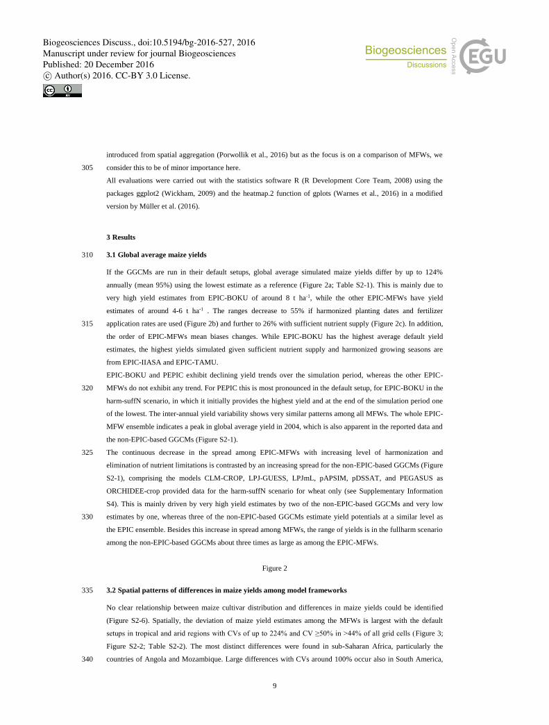
If the GGCMs are run in their default setups, global average simulated maize yields differ by up to 124%

annually (mean 95%) using the lowest estimate as a reference (Figure 2a; Table S2-1). This is mainly due to

very high yield estimates from EPIC-BOKU of around 8 t ha-1, while the other EPIC-MFWs have yield

estimates of around 4-6 t ha-1 . The ranges decrease to 55% if harmonized planting dates and fertilizer

application rates are used (Figure 2b) and further to 26% with sufficient nutrient supply (Figure 2c). In addition, 315

the order of EPIC-MFWs mean biases changes. While EPIC-BOKU has the highest average default yield

estimates, the highest yields simulated given sufficient nutrient supply and harmonized growing seasons are

from EPIC-IIASA and EPIC-TAMU.

EPIC-BOKU and PEPIC exhibit declining yield trends over the simulation period, whereas the other EPIC-

MFWs do not exhibit any trend. For PEPIC this is most pronounced in the default setup, for EPIC-BOKU in the 320

harm-suffN scenario, in which it initially provides the highest yield and at the end of the simulation period one

of the lowest. The inter-annual yield variability shows very similar patterns among all MFWs. The whole EPIC-

MFW ensemble indicates a peak in global average yield in 2004, which is also apparent in the reported data and

the non-EPIC-based GGCMs (Figure S2-1).

The continuous decrease in the spread among EPIC-MFWs with increasing level of harmonization and 325

elimination of nutrient limitations is contrasted by an increasing spread for the non-EPIC-based GGCMs (Figure

S2-1), comprising the models CLM-CROP, LPJ-GUESS, LPJmL, pAPSIM, pDSSAT, and PEGASUS as

ORCHIDEE-crop provided data for the harm-suffN scenario for wheat only (see Supplementary Information

S4). This is mainly driven by very high yield estimates by two of the non-EPIC-based GGCMs and very low

estimates by one, whereas three of the non-EPIC-based GGCMs estimate yield potentials at a similar level as 330

the EPIC ensemble. Besides this increase in spread among MFWs, the range of yields is in the fullharm scenario

among the non-EPIC-based GGCMs about three times as large as among the EPIC-MFWs.

Figure 2

3.2 Spatial patterns of differences in maize yields among model frameworks 335

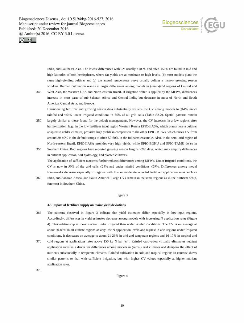
No clear relationship between maize cultivar distribution and differences in maize yields could be identified

(Figure S2-6). Spatially, the deviation of maize yield estimates among the MFWs is largest with the default

setups in tropical and arid regions with CVs of up to 224% and CV ≥50% in >44% of all grid cells (Figure 3;

Figure S2-2; Table S2-2). The most distinct differences were found in sub-Saharan Africa, particularly the

countries of Angola and Mozambique. Large differences with CVs around 100% occur also in South America, 340


10

India, and Southeast Asia. The lowest differences with CV usually <100% and often <50% are found in mid and

high latitudes of both hemispheres, where (a) yields are at moderate or high levels, (b) most models plant the

same high-yielding cultivar and (c) the annual temperature curve usually defines a narrow growing season

window. Rainfed cultivation results in larger differences among models in (semi-)arid regions of Central and

West Asia, the Western USA and North-eastern Brazil. If irrigation water is applied by the MFWs, differences 345

increase in most parts of sub-Saharan Africa and Central India, but decrease in most of North and South

America, Central Asia, and Europe.

Harmonizing fertilizer and growing season data substantially reduces the CV among models to ≤64% under

rainfed and ≤54% under irrigated conditions in 75% of all grid cells (Table S2-2). Spatial patterns remain

largely similar to those found for the default managements. However, the CV increases in a few regions after 350

harmonization. E.g., in the low fertilizer input region Western Russia EPIC-IIASA, which plants here a cultivar

adapted to colder climates, provides high yields in comparison to the other EPIC-MFWs, which raises CV from

around 30-40% in the default setups to often 50-60% in the fullharm ensemble. Also, in the semi-arid region of

North-eastern Brazil, EPIC-IIASA provides very high yields, while EPIC-BOKU and EPIC-TAMU do so in

Southern China. Both regions have reported growing season lengths >200 days, which may amplify differences 355

in nutrient application, soil hydrology, and planted cultivars.

The application of sufficient nutrients further reduces differences among MFWs. Under irrigated conditions, the

CV is now in 50% of the grid cells ≤25% and under rainfed conditions ≤29%. Differences among model

frameworks decrease especially in regions with low or moderate reported fertilizer application rates such as

India, sub-Saharan Africa, and South America. Large CVs remain in the same regions as in the fullharm setup, 360

foremost in Southern China.

Figure 3

3.3 Impact of fertilizer supply on maize yield deviations

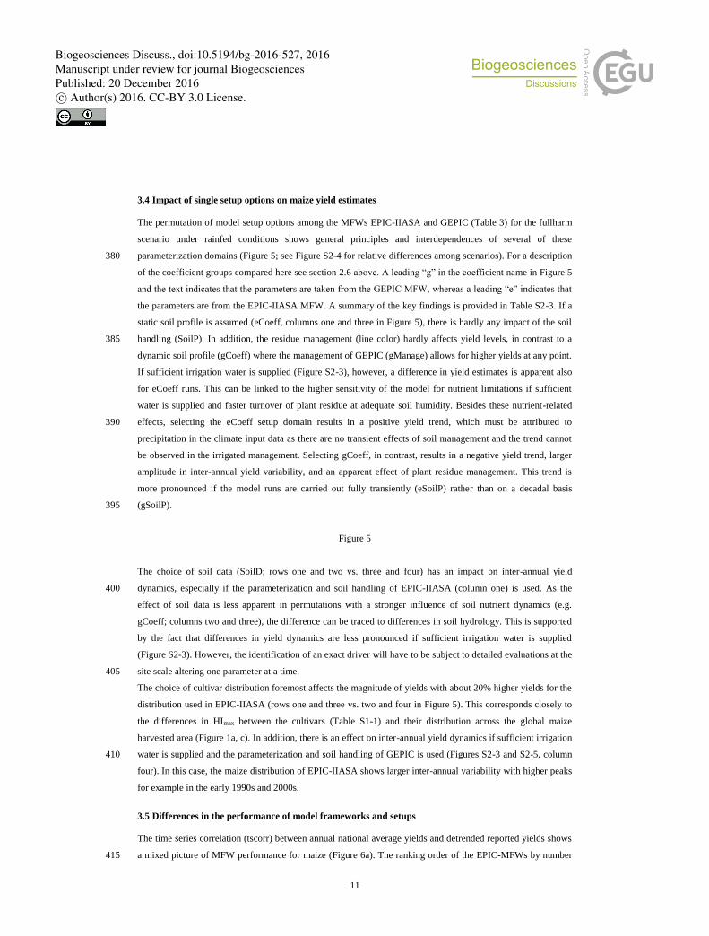
The patterns observed in Figure 3 indicate that yield estimates differ especially in low-input regions. 365

Accordingly, differences in yield estimates decrease among models with increasing N application rates (Figure

4). This relationship is more evident under irrigated than under rainfed conditions. The CV is on average at

about 60-85% in all climate regions at very low N application levels and highest in arid regions under irrigated

conditions. It decreases on average to about 21-23% in arid and temperate regions and 16-17% in tropical and

cold regions at applications rates above 150 kg N ha-1 yr-1. Rainfed cultivation virtually eliminates nutrient 370

application rates as a driver for differences among models in (semi-) arid climates and dampens the effect of

nutrients substantially in temperate climates. Rainfed cultivation in cold and tropical regions in contrast shows

similar patterns to that with sufficient irrigation, but with higher CV values especially at higher nutrient

application rates.

375

Figure 4


11

3.4 Impact of single setup options on maize yield estimates

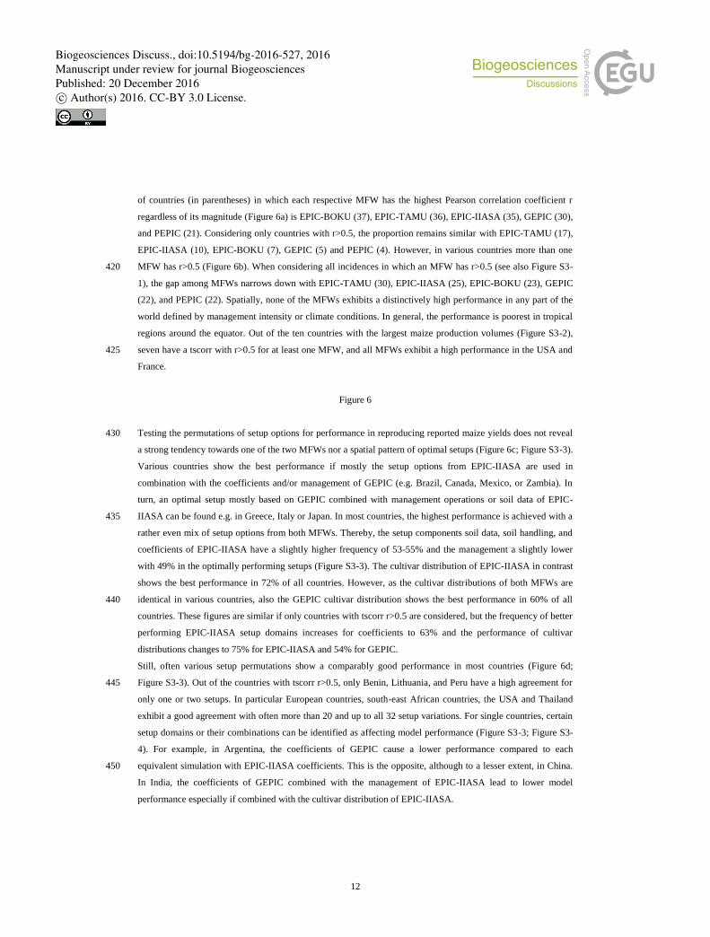
The permutation of model setup options among the MFWs EPIC-IIASA and GEPIC (Table 3) for the fullharm

scenario under rainfed conditions shows general principles and interdependences of several of these

parameterization domains (Figure 5; see Figure S2-4 for relative differences among scenarios). For a description 380

of the coefficient groups compared here see section 2.6 above. A leading “g” in the coefficient name in Figure 5

and the text indicates that the parameters are taken from the GEPIC MFW, whereas a leading “e” indicates that

the parameters are from the EPIC-IIASA MFW. A summary of the key findings is provided in Table S2-3. If a

static soil profile is assumed (eCoeff, columns one and three in Figure 5), there is hardly any impact of the soil

handling (SoilP). In addition, the residue management (line color) hardly affects yield levels, in contrast to a 385

dynamic soil profile (gCoeff) where the management of GEPIC (gManage) allows for higher yields at any point.

If sufficient irrigation water is supplied (Figure S2-3), however, a difference in yield estimates is apparent also

for eCoeff runs. This can be linked to the higher sensitivity of the model for nutrient limitations if sufficient

water is supplied and faster turnover of plant residue at adequate soil humidity. Besides these nutrient-related

effects, selecting the eCoeff setup domain results in a positive yield trend, which must be attributed to 390

precipitation in the climate input data as there are no transient effects of soil management and the trend cannot

be observed in the irrigated management. Selecting gCoeff, in contrast, results in a negative yield trend, larger

amplitude in inter-annual yield variability, and an apparent effect of plant residue management. This trend is

more pronounced if the model runs are carried out fully transiently (eSoilP) rather than on a decadal basis

(gSoilP). 395

Figure 5

The choice of soil data (SoilD; rows one and two vs. three and four) has an impact on inter-annual yield

dynamics, especially if the parameterization and soil handling of EPIC-IIASA (column one) is used. As the 400

effect of soil data is less apparent in permutations with a stronger influence of soil nutrient dynamics (e.g.

gCoeff; columns two and three), the difference can be traced to differences in soil hydrology. This is supported

by the fact that differences in yield dynamics are less pronounced if sufficient irrigation water is supplied

(Figure S2-3). However, the identification of an exact driver will have to be subject to detailed evaluations at the

site scale altering one parameter at a time. 405

The choice of cultivar distribution foremost affects the magnitude of yields with about 20% higher yields for the

distribution used in EPIC-IIASA (rows one and three vs. two and four in Figure 5). This corresponds closely to

the differences in HImax between the cultivars (Table S1-1) and their distribution across the global maize

harvested area (Figure 1a, c). In addition, there is an effect on inter-annual yield dynamics if sufficient irrigation

water is supplied and the parameterization and soil handling of GEPIC is used (Figures S2-3 and S2-5, column 410

four). In this case, the maize distribution of EPIC-IIASA shows larger inter-annual variability with higher peaks

for example in the early 1990s and 2000s.

3.5 Differences in the performance of model frameworks and setups

The time series correlation (tscorr) between annual national average yields and detrended reported yields shows

a mixed picture of MFW performance for maize (Figure 6a). The ranking order of the EPIC-MFWs by number 415


12

of countries (in parentheses) in which each respective MFW has the highest Pearson correlation coefficient r

regardless of its magnitude (Figure 6a) is EPIC-BOKU (37), EPIC-TAMU (36), EPIC-IIASA (35), GEPIC (30),

and PEPIC (21). Considering only countries with r>0.5, the proportion remains similar with EPIC-TAMU (17),

EPIC-IIASA (10), EPIC-BOKU (7), GEPIC (5) and PEPIC (4). However, in various countries more than one

MFW has r>0.5 (Figure 6b). When considering all incidences in which an MFW has r>0.5 (see also Figure S3-420

1), the gap among MFWs narrows down with EPIC-TAMU (30), EPIC-IIASA (25), EPIC-BOKU (23), GEPIC

(22), and PEPIC (22). Spatially, none of the MFWs exhibits a distinctively high performance in any part of the

world defined by management intensity or climate conditions. In general, the performance is poorest in tropical

regions around the equator. Out of the ten countries with the largest maize production volumes (Figure S3-2),

seven have a tscorr with r>0.5 for at least one MFW, and all MFWs exhibit a high performance in the USA and 425

France.

Figure 6

Testing the permutations of setup options for performance in reproducing reported maize yields does not reveal 430

a strong tendency towards one of the two MFWs nor a spatial pattern of optimal setups (Figure 6c; Figure S3-3).

Various countries show the best performance if mostly the setup options from EPIC-IIASA are used in

combination with the coefficients and/or management of GEPIC (e.g. Brazil, Canada, Mexico, or Zambia). In

turn, an optimal setup mostly based on GEPIC combined with management operations or soil data of EPIC-

IIASA can be found e.g. in Greece, Italy or Japan. In most countries, the highest performance is achieved with a 435

rather even mix of setup options from both MFWs. Thereby, the setup components soil data, soil handling, and

coefficients of EPIC-IIASA have a slightly higher frequency of 53-55% and the management a slightly lower

with 49% in the optimally performing setups (Figure S3-3). The cultivar distribution of EPIC-IIASA in contrast

shows the best performance in 72% of all countries. However, as the cultivar distributions of both MFWs are

identical in various countries, also the GEPIC cultivar distribution shows the best performance in 60% of all 440

countries. These figures are similar if only countries with tscorr r>0.5 are considered, but the frequency of better

performing EPIC-IIASA setup domains increases for coefficients to 63% and the performance of cultivar

distributions changes to 75% for EPIC-IIASA and 54% for GEPIC.

Still, often various setup permutations show a comparably good performance in most countries (Figure 6d;

Figure S3-3). Out of the countries with tscorr r>0.5, only Benin, Lithuania, and Peru have a high agreement for 445

only one or two setups. In particular European countries, south-east African countries, the USA and Thailand

exhibit a good agreement with often more than 20 and up to all 32 setup variations. For single countries, certain

setup domains or their combinations can be identified as affecting model performance (Figure S3-3; Figure S3-

4). For example, in Argentina, the coefficients of GEPIC cause a lower performance compared to each

equivalent simulation with EPIC-IIASA coefficients. This is the opposite, although to a lesser extent, in China. 450

In India, the coefficients of GEPIC combined with the management of EPIC-IIASA lead to lower model

performance especially if combined with the cultivar distribution of EPIC-IIASA.


13

4 Discussion

4.1 Crop distributions and parameterizations in the model frameworks

The analyses performed here do not allow for identifying optimal maize cultivar distributions based on the 455

EPIC-MFWs yield estimates and observations. This is due to the wide range of differences among EPIC-MFW

setups and will hence have to be subject of a focus study. From a general point of view, each of the four

approaches for spatially distributing maize cultivars (in terms of optimum temperature ranges and HI as defined

in Table S1-1) globally used by the EPIC-MFWs follows logical rules but with differing rationales. The zoning

approach based on agro-climatic and economic regions used in EPIC-IIASA (Figure 1a) accounts for climatic 460

adaptation of cultivars as well as access to improved seeds. Using reported long-term yield dynamics to

distribute maize cultivars as in EPIC-TAMU (Figure 1b) takes processes in agricultural development into

account. The HDI used in GEPIC and PEPIC (Figure 1c) reflects socio-economic means for investing in

improved inputs and access to knowledge. Finally, planting the same cultivar globally as done in EPIC-BOKU

(Figure 1d) ensures high spatial comparability of plant growth processes in the model. However, none of the 465

approaches can be considered to fully reflect the actual distribution of maize cultivars, including the challenging

problem of sub-grid heterogeneity. Already the fact that there are strongly differing domestic agricultural

systems in large transition countries like Brazil, China and India implies the requirement for a more nuanced

approach of distributing cultivars. As neither the national, nor the subnational, socio-economic situation can

fully serve as a proxy for agricultural management intensities, a global characterization of agricultural 470

production systems will be required to develop a valid dataset for current maize cultivar distributions. Such a

baseline distribution, along with characterization of the drivers will also be a crucial first step for developing

realistic projections of future cultivar distribution under environmental change.

4.2 Drivers for differences in maize yield estimates

4.2.1 General setup components 475

The largest differences for global average maize yield estimates among EPIC-MFWs in their default setups

(Figure 2) result from the planting of a high-yielding cultivar and uniformly high fertilizer supply in EPIC-

BOKU, contrasted by present fertilizer inputs and expansive planting of a low-yielding cultivar in GEPIC and

PEPIC. The inclusion of a dynamic soil profile and soil erosion in the latter two further adds to this. EPIC-

IIASA and EPIC-TAMU have lower extents for planting the low-yielding cultivar and use a static soil profile 480

and/or full water erosion control in their setups. In contrast to the other EPIC-MFWs, PEPIC exhibits a negative

yield trend over time. This can be attributed to the use of fixed fertilizer application schedule in PEPIC (see

section 2.2.5) in contrast to automatic application based on plant requirements in the other EPIC-MFWs, which

typically increase nutrient losses, and the inclusion of soil erosion combined with fully transient model runs.

Both of which have been shown to affect yield trends in the model before (Liu et al., 2016b). The fact that the 485

mean bias among EPIC-MFWs becomes very small with sufficient nutrient supply highlights that nutrient

supply is the main driver for differences in mean model bias. However, the remaining differences in inter-annual

yield variability indicate that yield estimates in individual years are not only affected by climate but also

strongly by additional factors such as parameterization of soil hydrology and evapotranspiration, cultivars, and

timing of irrigation water supply. 490


14

The facts that the non-EPIC-based GGCM ensemble shows a relative increase in the mean range of yield

estimates with increasing level of harmonization and that the spread among non-EPIC-based GGCMs in the

fullharm scenario is about three times the spread among the EPIC-based MFWs (Figure S2-1) highlight that the

uncertainty introduced by differences in parameterization and input data in the same model is still far lower than

uncertainties related to conceptual differences among models. These have been characterized in Müller et al. 495

(2016) and on https://www.isimip.org/impactmodels. General differences such as the inclusion of certain

climate variables and employment of contrasting representations of photosynthesis and biomass partitioning

may have less of an effect on this phenomenon. More importantly, the models take soil characteristics (and

hence their limiting effects) into account at varying levels of detail, have cultivars based on plant functional

types or specific crop cultivars, and have explicit representations of nutrient supply or include these through 500

aggregated management coefficients. In addition, several of the GGCMs have been calibrated to reproduce

present yield levels in their default setups, either by altering such management coefficients, or by fitting the crop

phenology. In these cases, changing growing season and fertilizer input data typically results in new

combinations of these fitted variables and agronomic conditions, which can cause the observed yield estimates

far above or below the reported levels despite the good fit in the default setups. The EPIC model in contrast was 505

specifically developed to investigate impacts of crop management on yields and due to the same set of

algorithms employed in the EPIC-MFWs an increasingly good fit could be expected with increasing level of

harmonization.

4.2.2 Spatial differences among model frameworks and effects on yield estimates

Spatially, low yields and tropical climate are characteristic of regions in which the EPIC-MFWs show large 510

differences in maize yield estimates in their default setups (Figure 3). The large CV is in part a result of the low

yield estimates in EPIC-IIASA, EPIC-TAMU, GEPIC and PEPIC, resulting in a low mean yield, but is mainly

due to the estimation of yield potential by EPIC-BOKU (Figure 2a). Besides fertilizer inputs, assumptions about

growing seasons differ more strongly in tropic and warm arid regions, where cropping is often possible

throughout the whole year, in contrast to temperate and cold climates which usually provide only a narrow 515

growing-season window. The fact that irrigation increases differences among EPIC-MFWs in parts of sub-

Saharan Africa and India is mostly due to further increases of non-nutrient-limited yield potential estimates in

EPIC-BOKU. An additional minor effect is the elimination of plant water stress, which amplifies differences

among the other EPIC-MFWs due to a higher sensitivity of EPIC to differences in nutrient supply (see Sect.

2.1). This is most pronounced in low-input regions, where nutrient supply depends on the parameterization of 520

soil nutrient cycling and crop residue management.

The harmonization of annual nutrient application rates and growing season dates decreases the differences

among EPIC-MFWs substantially. The main driver is the adoption of reported fertilizer application rates in

EPIC-BOKU. The effect is hence largest in present low-input regions such as sub-Saharan Africa, South

America and parts of Asia. The larger differences under rainfed conditions - mostly in (semi-)arid regions - may 525

be attributed to differences in soil hydrology based on differing soil data, tillage and residue management, and

the parameterization of soil and runoff processes, all of which affect plant water availability (see Folberth et al.,

2016). Smaller differences remain in Europe, the USA, Oceania, Japan and southern South America where the

predominant use of high-yielding maize cultivars is reflected in all MFWs.


15

The application of sufficient nutrients mostly leaves CV<40% for maize yields among models. The remaining 530

difference can to a large extent be explained by the use of different maize cultivars, which differ by about 50%

in genetic yield potential if the lower value is used as a base. As nutrient supply from the soil is virtually

eliminated in this management scenario, factors affecting plant available water, such as estimation routines for

PET, runoff, and soil hydrology (Table 1) also contribute to remaining uncertainties. If sufficient irrigation

water is supplied, major differences in setups remain in fertilizer (threshold for automatic application or timing 535

of rigid application) and irrigation water (threshold for automatic application and maximum volumes)

application.

Although the CV among EPIC-MFWs decreases substantially with harmonization of growing seasons and

fertilizer rates, and further with application of sufficient nutrients, the global deviation among crop yield

estimates is still too large to allow for a detailed quantification or ranking of drivers in these deviations. For 540

example, low yields may occur as well if a high-yielding cultivar is planted and soil nutrients are depleted (e.g.

from long-term cultivation or soil erosion) or if a low-yielding cultivar is planted and moderate amounts of

fertilizer are applied (see Folberth et al., 2012). Substantial differences remain among the model setups when it

comes to processed soil data, soil nutrient cycling and the handling of crop residues after harvest. All of these

are major determinants for nutrient availability if exogenous nutrient application is low or completely lacking. 545

The remaining differences among yield estimates highlight that a further harmonization may need to prioritize

the handling of fertilizer application (i.e. thresholds for automatic application or timing for fixed rates) in the

MFWs besides the parameterization of soil nutrient dynamics, soil data itself and the handling of crop residues.

Recently, the substantial impact of soil type selection in the EPIC framework GEPIC has been evaluated in

detail by Folberth et al. (2016) showing that soil data can drive absolute yield levels as well as inter-annual yield 550

dynamics and the crop’s sensitivity to adverse climate conditions. While a harmonization of soil data is difficult

across a range of GGCMs with highly differing conceptual treatment of soil processes and required variables,

phase 2 of the GGCMI project prescribes a rigid fertilizer application schedule to eliminate this source of

uncertainty.

The largest differences remain in the tropics, thus highlighting the need for more extensive model evaluations 555

and data collection in these regions. Continuous high temperatures and humidity levels in the tropics allow for a

rapid turnover of organic material like plant residue. At the same time, mineral nutrient application rates are

often low in these regions, i.e. most of Sub-Saharan Africa and parts of South America. The parameterization of

these turnover processes can here be a key factor for minimizing differences among EPIC-MFWs, which is also

indicated by the large differences among EPIC-MFWs in low-input grid cells (Figure 4). Furthermore, we find 560

the distribution of maize cultivars among EPIC-MFWs differs the most in these regions. This input can be

considered a priority for harmonization when it comes to reproducing absolute yield levels but - due to

differences in water stress sensitivity among different cultivars - also in the estimation of inter-annual yield

variability.

Concerning the cold and temperate zones, a recent study based on PEPIC has shown that the choice of the PET 565

estimation method causes the largest differences in these regions (Liu et al., 2016a). It will hence need to be

tested, how an ensemble of GGCMs reacts to different choices of PET estimation methods.


16

4.3 Impact of single setup domains on maize yield estimates

The comparison of EPIC-IIASA and GEPIC shows that both EPIC-MFWs are capable of producing fairly stable

yield levels over time within their respective setups, which is essential for estimating climate change impacts on 570

crop yields without bias from trends in soil quality. However, they differ substantially in magnitudes of yields as

well as in inter-annual yield variability. The latter can be traced to (a) the use of static vs dynamic soil profiles,

(b) cultivars with different water stress sensitivity, and most importantly (c) the parameterization and choices of

subroutines as specified in Table 1.

Both EPIC-MFWs use the Hargreaves method (Hargreaves and Samani, 1985) to estimate PET, but with 575

different parameterizations. GEPIC uses the original exponential coefficient and a linear coefficient that had

been adjusted by the EPIC developers for prior studies. Vice versa, EPIC-IIASA uses the original value for the

linear coefficient and an adjusted exponential coefficient. Neither of the two parameterizations can be

considered more favorable than the other for global-scale applications, as PET estimation methods in general

require a local calibration (e.g. Gavilán et al., 2006). This is presently not feasible at the global scale due to lack 580

of validation data. The selected parameter values cause higher PET in GEPIC at low to moderate daily

temperature ranges, especially at high average temperatures and higher PET in EPIC-IIASA at high diurnal

temperature ranges. An effect is that GEPIC has a higher likeliness of water stress in most climate regions,

except for deserts and mountain ranges, where large differences in day and night time temperatures are

common. In addition, the soil evaporation coefficient had been lowered in EPIC-IIASA from its default value, 585

which decreases the fraction of ET evaporating from soils. All these hydrologic factors contribute to differences

among the EPIC-MFWs in inter-annual yield variability when comparing columns one and two or three and four

of Figure 5 and Figure S2-4.

As the parameterizations of the two EPIC-MFWs were exchanged collectively, however, other parameters

discussed above for the whole ensemble such as plant stress thresholds for fertilizer application and coefficients 590

for microbial turnover of soil organic matter (SOM) also play a role here. The upper limit for denitrification was

set very low in GEPIC due to prior applications for sub-Saharan Africa based on a calibration of the EPIC

model for the region (Gaiser et al., 2010), whereas denitrification was allowed to be high in EPIC-IIASA. The

microbial decay rate, a coefficient for turnover rates of SOM, in contrast, was strongly limited in EPIC-IIASA

and set to a default value corresponding to no limitations due to microbial activity in GEPIC. The latter causes 595

more rapid mineralization of nutrients from SOM. This drives differences between the two MFWs regarding

residue management and nutrient cycling. Also the option of using a dynamic or a static soil profile contributes

substantially to crop yield estimates. Depending on the climate and management, the static soil profile can in

each year potentially provide the same amount of nutrients from SOM mineralization whereas the dynamic soil

profile will experience soil nutrient depletion in low-input regions before being reset after a decade (see 600

Supplementary 1). This may cause the overall more negative yield trends in the gCoeff scenarios and contributes

to differences in inter-annual yield variability due to diverging handling of soil structure and SOM across

growing seasons.

The soil data used in the two models are based on the same dataset but have been aggregated to different

standardized soil profiles for EPIC-IIASA as described in Sect. 2.3. Still, organic carbon (OC) contents are 605

identical in >75% and within a range of ±20% in nearly 90% of all grid cells globally, which renders nutrient

availability from initial SOM a minor determinant for differences in yield estimates (not shown). A major


17

difference is that water content at field capacity and wilting point, as well as hydraulic conductivity, are being

estimated by different pedotransfer functions in the two MFWs (Table 1). This causes on average about 10%

higher rainfed yield estimates in EPIC-IIASA (Figure 5, column one), an effect that is largely cancelled if 610

sufficient irrigation water is supplied (Figure S2-3 and Figure S2-5, column one), and emphasizes the

importance of high resolution and quality soil data, as well as also raising questions about how to handle sub-

grid heterogeneity in such parameters (e.g. Folberth et al., 2016).

The cultivar distribution predominantly scales absolute yield levels. Based on HImax of the cultivars and their

coverage within the two MFWs, the genetic yield potential is 19% lower in the GEPIC dataset than in EPIC-615

IIASA. This corresponds closely to the difference observed among the corresponding yield estimates (Figure 5,

rows one and three vs. two and four). The HImin under water stress for cultivar 1 affects yield estimates only

under severe water stress. This influences the inter-annual yield variability by causing disproportionately lower

yields in extremely dry years. Apart from the HI also the temperature response of cultivar 3 used in the EPIC-

IIASA setup has an impact on crop phenology and hence inter-annual yield variability. The performance when 620

using the EPIC-IIASA cultivar distribution if better in various Eurasian countries in which this cultivar is

planted, such as Albania, Austria, Czech Republic, Germany, Luxembourg, Moldova, and Slovakia (Figure S3-

3). However, also the default cultivar 1 used in GEPIC in the same region shows in some instances a better

performance, e.g. in Belgium, Bulgaria, and Greece.

4.4 Model framework performances in estimating reported crop yields 625

As the variability in observed national yield time series is often also driven by non-weather related variability of

unknown importance, GGCMs cannot be expected to explain yield variability in all countries. Müller et al.

(2016) established a first benchmark for GGCM performance where the EPIC-MFWs show similar performance

to the other GGCMs in that study. Here, a good agreement between estimated and reported yields was found for

various major producing countries, where fertilizer inputs are usually moderate to high and stable harvest area 630

distributions within countries (as assumed in the constant global harvested areas dataset used for evaluations)

can be expected In low-input regions in contrast, there is commonly little agreement with reported yields. This

has various reasons such as (a) management may be very particular, e.g. slash and burn agriculture or crop

rotations that are commonly not reflected in the GGCMs, (b) yields depend strongly on agro-environmental

processes such as nutrient cycling, (c) plant protection measures are often low, rendering the impact of pests and 635

diseases larger than in high-input regions, (d) yields reported in global databases have often been estimated, and

(e) cultivars may be highly adapted to local environmental conditions and consumer preferences. In addition, the

fact that EPIC takes only the major stress (out of nutrient deficit, water deficit, adverse temperature, and limited

root aeration) on each day of the growing season into account to limit biomass production implies interactions

between nutrient input levels and the model’s sensitivity to weather-induced stresses. This approach thus lowers 640

the crop’s sensitivity to water and temperature stress if nutrient deficits are prevailing.

General conclusions as to which setup factors improve the performance in certain countries are challenging to

draw. The setup options represent highly aggregated domains with more than 20 parameters included in the

coefficient setup domain alone (Table 1). One setup factor that can clearly be identified to allow for higher

performance in Argentina and India are the coefficients of EPIC-IIASA, which result in all 16 combinations in a 645

tscorr with r>0.5 (Figure S3-4). However, in both countries there are also two setups based on the


18

parameterization of GEPIC in combination with GEPIC’s soil handling that allow for r>0.5. Vice versa, the

parameterization of EPIC-IIASA causes a worse performance in Brazil if combined with the soil data of EPIC-

IIASA, but a high tscorr if combined with the cultivar and soil data of GEPIC. The most dramatic contrast in

setups and their performance is found in Indonesia and Ukraine, where those resulting in higher performance in 650

the first cause lower performance in the latter, albeit none of the scenarios yields r>0.5. Identifying country- or

region-specific optimal setups will hence require an even wider range of setup permutations, ideally based on

more detailed datasets or the inclusion of findings from local and field-scale model studies that allow for

reducing the dimensions of such an exercise. Also, the different setups can represent part of the variability in

management systems that are present in actual production systems but greatly underrepresented in modelled 655

production systems.

Besides setups and algorithms of the models, also input data (e.g. Ruane et al., in preparation), validation data

(Müller et al., 2016), and landuse masks (Porwollik et al., 2016) affect model performance, complicating its

evaluation (see Müller et al. 2016). Thus, the focus of this study was not on model performance per se, but

rather on identifying differences among EPIC-MFWs that substantially affect model performance. 660

5 Conclusions

The results presented herein highlight the limited comparability of outputs from various GGCMs based on the

same, or very similar, sets of biophysical algorithms, but with differences in parameterizations and management

assumptions. This has implications as well for (a) the preparation of common input data for future ensemble

runs aiming at the identification of differences in model algorithms globally, and (b) the interpretability of 665

GGCM-based studies. On the other hand, the EPIC-based ensemble shows better agreement in terms of mean

model bias if certain aspects of model uncertainty are eliminated (growing seasons, fertilizer application levels,

and soil nutrient supply), in contrast to a non-EPIC-based ensemble which shows increasing bias.

The differences in model outputs induced by differences in setups indicate that further steps of harmonization

among GGCMs should be taken if model algorithms are to be compared globally. However, prioritizing and 670

selecting input data for further harmonization of the whole ensemble is not a straightforward process. None of

the MFWs evaluated herein exhibited an outstanding performance in reproducing reported yields that would

allow for justifying the selection of its maize cultivar or wheat type distribution. In order to overcome issues

related to the wheat type distribution, following phases of the GGCMI project will collect winter and spring

wheat simulations separately for regions in which both may be grown in order to allow for ex-post distributions 675

according to wheat type masks. A harmonization of major maize cultivars appears less feasible in the short run

due to differing scopes among research groups. Although the cultivar distribution of EPIC-IIASA performs

overall better than that of GEPIC, it is as well not optimal in all regions. Producing global cultivar distribution

maps may hence require the compilation of a global inventory of representative maize cultivars and their

geographic distribution. Soil data will need to be harmonized to avoid differences in nutrient supply in low-input 680

regions from SOM mineralization and especially differences in soil hydrology in regions with low precipitation

under rainfed growth conditions. While a compilation of global crop management practices cannot be expected

in the short run, management practices regarding the timing of fertilizer application and thresholds for automatic

fertilizer and water irrigation need to be harmonized to avoid deviations among GGCMs impairing the

interpretability of plant water stress. To address this issue, model runs in GGCMI phase 2 will be performed 685


19

with prescribed timing and rates of fertilizer application. Plant residue management can differ substantially from

farm to farm as it is subject to farm type and socio-economic drivers and may hence rather be addressed by

scenario analyses in future GGCM studies.

Further harmonization of GGCMs in terms of subroutines and parameterization, on the other hand, can be

expected to become a long-term process and care must be taken to ensure that the harmonized variables are a 690

genuinely improved representation of reality, and not just a more limited sampling of the uncertainty space.

Single parameters and subroutines such as PET estimation methods or microbial turnover processes are often

representative for specific climatic and agro-ecologic regions. However, up to now they cannot be attributed

spatially based on any available covariates in global datasets. Hence, running a range of MFWs based on the

same field-scale model in different parameterizations allows meanwhile to bracket likely yield estimates by 695

covering gaps in the understanding of agro-environmental processes. Further regional and field assessments, in

combination with climate and pedologic zoning, will be required to derive reasonable spatially explicit datasets

on the optimal PET estimation method, parameterization of microbial activity, and common SOM turn-over

rates among others.

700

Data availability

Model output data will be made available via the GGCMI data archive.

Acknowledgements

We acknowledge the support and data provision by the Agricultural Intercomparison and Improvement Project 705

(AgMIP). AA and TAMP were funded by the European Commission’s 7th Framework Programme, under Grant

Agreement number 603542 (LUC4C). CF, JB, NK, and RS were supported by the European Research Council

Synergy Grant number ERC-2013-SynG-610028 (IMBALANCE-P).

References

Asseng, S., Ewert, F., Rosenzweig, C., Jones, J. W., Hatfield, J. L., Ruane, A. C., Boote, K. J., Thorburn, P. J., 710

Rotter, R. P., Cammarano, D., Brisson, N., Basso, B., Martre, P., Aggarwal, P. K., Angulo, C.,

Bertuzzi, P., Biernath, C., Challinor, A. J., Doltra, J., Gayler, S., Goldberg, R., Grant, R., Heng, L.,

Hooker, J., Hunt, L. A., Ingwersen, J., Izaurralde, R. C., Kersebaum, K. C., Muller, C., Naresh Kumar,

S., Nendel, C., O/'Leary, G., Olesen, J. E., Osborne, T. M., Palosuo, T., Priesack, E., Ripoche, D.,

Semenov, M. A., Shcherbak, I., Steduto, P., Stockle, C., Stratonovitch, P., Streck, T., Supit, I., Tao, F., 715

Travasso, M., Waha, K., Wallach, D., White, J. W., Williams, J. R., and Wolf, J.: Uncertainty in

simulating wheat yields under climate change, Nat. Clim. Change, 3, 827-832, 2013.

Balkovič, J., van der Velde, M., Schmid, E., Skalský, R., Khabarov, N., Obersteiner, M., Stürmer, B., and

Xiong, W.: Pan-European crop modelling with EPIC: implementation, up-scaling and regional crop

yield validation. Agric. Syst., 120, 61-75, 2013. 720

Balkovič, J., van der Velde, M., Skalský, R., Xiong, W., Folberth, C., Khabarov, N., Smirnov, A., Mueller, N.

D., and Obersteiner, M.: Global wheat production potentials and management flexibility under the

representative concentration pathways, Glob. Planet. Change, 122, 107-121, 2014.


20

Batjes, N.H.: ISRIC-WISE derived soil properties on a 5 by 5 arc-minutes global grid. ISRIC - World Soil

Information, Wageningen, Netherlands, 2006. 725

Curtis, B. C.: Wheat in the world. in: Curtis, B. C., Rajaram, S., and Gómez Macpherson, H.: Bread Wheat

Improvement and Production. Food and Agriculture Organization of the United Nations, Rome, 2002.

Dee, D. P., Uppala, S. M., Simmons, A. J., Berrisford, P., Poli, P., Kobayashi, S., Andrae, U., Balmaseda, M.

A., Balsamo, G., Bauer, P., and Bechtold, P.: The ERA-Interim reanalysis: configuration and

performance of the data assimilation system:. Q. J. R. Meteorol. Soc., 137, 553-597, 2011. 730

Deryng, D., Sacks, W. J., Barford, C. C., and Ramankutty, N.: Simulating the effects of climate and land

management practices on global crop yield, Global Biogeochem. Cycles, 25,

doi:10.1029/2009GB003765, 2011

Deryng, D., Elliott, J., Folberth, C., Müller, C., Pugh, T. A., Boote, K. J., Conway, D., Ruane, A. C., Gerten, D.,

Jones, J. W., Khabarov, N., , Olin, S., Schaphoff, S., Schmid, E., Yang, H., and Rosenzweig, C.: 735

Regional disparities in the beneficial effects of rising CO2 emissions on crop water productivity, Nat.

Clim. Change, 6, 786-790, 2016.

Elliott, J., Kelly, D., Chryssanthacopoulos, J., Glotter, M., Jhunjhnuwala, K., Best, N., Wilde, M., and Foster, I.:

The Parallel System for Integrating Impact Models and Sectors (pSIMS), Environ. Modell. Softw., 62,

509–516, 2014. 740

Elliott, J., Müller, C., Deryng, D., Chryssanthacopoulos, J., Boote, K. J., Büchner, M., Foster, I., Glotter, M.,

Heinke, J., Iizumi, T., Izaurralde, R. C., Mueller, N. D., Ray, D. K., Rosenzweig, C., Ruane, A. C., and

Sheffield, J.: The Global Gridded Crop Model Intercomparison: data and modeling protocols for Phase

1 (v1.0), Geosci. Model Dev., 8, 261-277, 2015.

Elshout, P. M. F., Van Zelm, R., Balkovič, J., Obersteiner, M., Schmid, E., Skalský, R., Van Der Velde, M., and 745

Huijbregts, M. A. J.: Greenhouse-gas payback times for crop-based biofuels, Nat. Clim. Change, 5,

604-610, 2015.

Fader, M., Rost, S., Müller, C., Bondeau, A., and Gerten, D.: Virtual water content of temperate cereals and

maize: present and potential future patterns, J. Hydrol. 384, 218–231, 2010.

FAO: FAO Digital Soil Map of the World, FAO, Rome, 1995. 750

FAO: FertiSTAT - Fertilizer Use Statistics, Food and Agricultural Organization of the UN, Rome, 2007.

FAO: FAOSTAT statistical database, Food and Agricultural Organization of the UN, Rome, 2014.

Folberth, C., Gaiser, T., Abbaspour, K. C., Schulin, R., and Yang, H.: Regionalization of a large-scale crop

growth model for sub-Saharan Africa: model setup, evaluation, and estimation of maize yields, Agr.

Ecosyst. Environ., 151, 21-33, 2012. 755

Folberth, C., Yang, H., Gaiser, T., Liu, J., Wang, X., Williams, J., and Schulin, R.: Effects of ecological and

conventional agricultural intensification practices on maize yields in sub-Saharan Africa under

potential climate change, Environ. Res. Lett., 9, 044004, 2014.

Folberth, C., Skalský, R., Moltchanova, E., Balkovič, J., Azevedo, L. B., Obersteiner, M., and van der Velde,

M.: Uncertainty in soil data can outweigh climate impact signals in global crop yield simulations, Nat. 760

Commun., 7, 11872, 2016.


21

Frank, S., Schmid, E., Havlík, P., Schneider, U.A., Balkovič, J., Obersteiner, M., and Böttcher, H.: The dynamic

soil carbon mitigation potential of European cropland, Global Environmental Change, 35, 269-278,

2015.

Havlík, P., Schneider, U. A., Schmid, E., Böttcher, H., Fritz, S., Skalský, R., Aoki, K., Cara, S. D., Kindermann, 765

G., Kraxner, F., Leduc, S., McCallum, I., Mosnier, A., Sauer, T., and Obersteiner, M.: Global land-use

implications of first and second generation biofuel targets, Energy Policy, 39, 5690–5702, 2011.

Gaiser, T., de Barros, I., Sereke, F., and Lange, F.-M.: Validation and reliability of the EPIC model to simulate

maize production in small-holder farming systems in tropical sub-humid West Africa and semi-arid

Brazil, Agr. Ecosyst. Environ., 135, 318-327, 2010. 770

Gassman, P. W., Williams, J. R., Benson, V. W., Izaurralde, R. C., Hauck, L. M., Jones, C. A., Atwood, J. D.,

Kiniry, J. R., and Flowers, J. D.: Historical Development and Applications of the EPIC and APEX

models, ASAE/CSAE Meeting Paper No. 042097, 2004.

Gavilán, P., Lorite, I. J., Tornero, S., and Berengena, J.: Regional calibration of Hargreaves equation for

estimating reference ET in a semiarid environment, Agr. Water Manage., 81, 257-281, 2006. 775

Gelfand, I., Sahajpal, R., Zhang, X., Izaurralde, R. C., Gross, K. L., and Robertson, G. P.: Sustainable bioenergy

production from marginal lands in the US Midwest, Nature, 493, 514-517, 2013.

Gbegbelegbe, S., Cammarano, D., Asseng, S., Robertson, Richard D., Chung, U., Adam, M., Abdalla, O.,

Payne, T., Reynolds, M., Sonder, K., Shiferaw, B., and Nelson, G. C.: Baseline simulation for global

wheat production with CIMMYT mega-environment specific cultivars, Field Crops Res., in press. 780

http://dx.doi.org/10.1016/j.fcr.2016.06.010, 2016

Gerik, T., Williams, J., Francis, L., Greiner, J., Magre, M., Meinardus, A., Steglich, E., and Taylor, R.:

Environmental Policy Integrated Climate Model - User’s Manual Version 0810, Blackland Research

and Extension Center, Texas A&M AgriLife, Temple, USA, 2014.

Hargreaves, G. H., and Samani, Z. A.: Reference crop evapotranspiration from temperature, Applied Engr. 785

Agric., 1, 96-99, 1985.

Hempel, S., Frieler, K., Warszawski, L., Schewe, J., and Piontek, F.: A trend-preserving bias correction - the

ISI-MIP approach, Earth Syst. Dynam., 4, 219-236, 2013.

Izaurralde, R. C., Williams, J. R., McGill, W. B., Rosenberg, N. J., and Quiroga Jakas, M. C.: Simulating soil C

dynamics with EPIC: model description and testing against long-term data, Ecol. Model., 192, 362-790

384, 2006.

Izaurralde, R. C., McGill, W. B., and Williams, J. R.: Development and application of the EPIC model for

carbon cycle, greenhouse gas mitigation, and biofuel studies, in: Liebig, M. A., Franzluebbers, A. J.,

and Follet, R. F.: Managing Agricultural Greenhouse Gases, Academic Press, San Diego, USA, 2012.

Kiniry, J. R., Major, D.J., Izaurralde, R.C., Williams, J.R., Gassman, P.W., Morrison, M., Bergentine, R., and 795

Zentner, R.P.: EPIC model parameters for cereal, oilseed, and forage crops in the northern Great Plains

region, Can. J. Plant Sci., 75, 679-688, 1995.

Kuhn, A., Gaiser, T., and Gandonou, E.: Simulating the effects of tax exemptions on fertiliser use in Benin by

linking biophysical and economic models, Agric. Syst., 103, 509-520, 2010.

Liu, J., Williams, J. R., Zehnder, A. J. B., and Yang, H.: GEPIC – modelling wheat yield and crop water 800

productivity with high resolution on a global scale, Agric. Syst., 94, 478-493, 2007.


22

Liu, J.: A GIS-based tool for modelling large-scale crop-water relations, Environ. Modell. Softw., 24, 411-422,

2009.

Liu, J., Folberth, C., Yang, H., Rockström, J., Abbaspour, K., and Zehnder, A. J. B.: A global and spatially

explicit assessment of climate change impacts on crop production and consumptive water use, PLoS 805

ONE, 8, e57750, 2013.

Liu, W., Yang, H., Folberth, C., Wang, X., Luo, Q., and Schulin, R.: Global investigation of impacts of PET

methods on simulating crop-water relations for maize, Agr. Forest. Meteorol., 221, 164-175, 2016a.

Liu, W., Yang, H., Liu, J., Azevedo, L. B., Wang, X., Xu, Z., Abbaspour, K. C., and Schulin, R.: Global

assessment of nitrogen losses and trade-offs with yields from major crop cultivations, Sci. Total 810

Environ., 572, 526-537, 2016b.

Lychuk, T. E., Izaurralde, R. C., Hill, R. L., McGill, W. B., and Williams, J. R.: Biochar as a global change

adaptation: predicting biochar impacts on crop productivity and soil quality with the EPIC model,

Mitig. Adapt. Strateg. Glob. Change, 20, 1437-1458, 2015.

McGill, W. B., Hunt, H. W., Woodmansee, R. G., and Reuss, J. O.: Phoenix, a model of the dynamics of carbon 815

and nitrogen in grassland soils, in: Clark, F. E. and Rosswall, T.: Terrestrial Nitrogen Cycles.

Processes, Ecosystem Strategies and Management Impacts, Ecological Bullettins, 49-115, Stockholm,

1981.

Mueller, N. D., Gerber, J. S., Johnston, M., Ray, D. K., Ramankutty, N., and Foley, J. A.: Closing yield gaps

through nutrient and water management, Nature, 490, 254-257, 2012. 820

Müller, C.: Agriculture: harvesting from uncertainties, Nature Clim. Change, 1, 253-254, 2011.

Müller, C., Elliott, J., Chryssanthacopoulos, J., Deryng, D., Folberth, C., Pugh, T. A., and Schmid, E.:

Implications of climate mitigation for future agricultural production, Environ. Res. Lett., 10, 125004,

2015.

Müller, C., Elliott, J., Chryssanthacopoulos, J., Arneth, A., Balkovič, J., Ciais, P., Deryng, D., Folberth, C., 825

Glotter, M., Hoek, S., Iizumi, T., Izaurralde, R. C., Jones, C., Khabarov, N., Lawrence, P., Liu, W.,

Olin, S., Pugh, T. A. M., Ray, D., Reddy, A., Rosenzweig, C., Ruane, A. C., Sakurai, G., Schmid, E.,

Skalský, R., Song, C. X., Wang, X., de Wit, A., and Yang, H.: Global Gridded Crop Model evaluation:

benchmarking, skills, deficiencies and implications, Geoscientific Model Development Discussions,

doi: 10.5194/gmd-2016-207, 2016. 830

Nelson, G. C., Valin, H., Sands, R. D., Havlík, P., Ahammad, H., Deryng, D., Elliott, J., Fujimori, S.,

Hasegawa, T., Heyhoe, E., Kyle, P., Von Lampe, M., Lotze-Campen, H., Mason d'Croz, D., van Meijl,

H., van der Mensbrugghe, D., Müller, C., Popp, A., Robertson, R., Robinson, S., Schmid, E., Schmitz,

C., Tabeau, A., and Willenbockel, D.: Climate change effects on agriculture: Economic responses to

biophysical shocks, Proc. Natl. Acad. Sci., 111, 3274-3279, 2014. 835

Nuttonson, M.Y.: Wheat-climatic relationships and the use of phenology in ascertaining the thermal and

photothermal requirements of wheat, American Institute of Crop Ecology, Washington, D. C., 1955.

Porwollik, V., Müller, C., Elliott, J., Chryssanthacopoulos, J., Iizumi, T., Ray, D. K., Ruane, A. C., Arneth, A.,

Balkovič, J., Ciais, P., Deryng, D., Folberth, C., Izaurralde, R. C., Jones, C. D., Khabarov, N.,

Lawrence, P. J., Liu, W., Pugh, T. A.M., Reddy, A., Sakurai, G., Schmid, E., Wang, X., de Wit, A., and 840


23

Wu, X.: Spatial and temporal uncertainty of crop yield aggregations, Eur. J. Agron., doi:

10.1016/j.eja.2016.08.006, 2016.

Portmann, F. T., Siebert, S., and Döll, P.: MIRCA2000 - Global monthly irrigated and rainfed crop areas around

the year 2000: A new high-resolution dataset for agricultural and hydrological modeling, Global

Biogeochem. Cy., 24, GB 1011, doi:10.1029/2008GB003435, 2010. 845

R Development Core Team: R: A language and environment for statistical computing, R Foundation for

Statistical Computing, Vienna, Austria, https://www.R-project.org, 2008.

Ray, D. K., Ramankutty, N., Mueller, N. D., West, P. C., and Foley, J. A.: Recent patterns of crop yield growth

and stagnation, Nat. Comm., 3, 1293, 2012.

Rosenzweig, C., Jones, J. W., Hatfield, J. L., Ruane, A. C., Boote, K. J., Thorburn, P., Antle, J. M., Nelson, G. 850

C., Porter, C., Janssen, S., Asseng, S., Basso, B., Ewert, F., Wallach, D., Baigorria, G., and Winter, J.

M.: The Agricultural Model Intercomparison and Improvement Project (AgMIP): Protocols and pilot

studies, Agr. Forest Meteorol., 170, 166-182, 2013.

Rosenzweig, C., Elliott, J., Deryng, D., Ruane, A. C., Arneth, A., Boote, K. J., Folberth, C., Glotter, M.,

Khabarov, N., Müller, C., Neumann, K., Piontek, F., Pugh, T., Schmid, E., Stehfest, E., and Jones, J. 855

W.: Assessing agricultural risks of climate change in the 21st century in a global gridded crop model

intercomparison, Proc. Natl. Acad. Sci., 111, 3268-3273, 2014.

Sacks, W.J., Deryng, D., Foley, J.A., and Ramankutty, N.: Crop planting dates: An analysis of global patterns,

Global Ecol. Biogeogr., 19, 607-620, 2010.

Schaap, M. G. and Bouten, W.: Modelling water retention curves of sandy soils using neural networks, Water 860

Resour. Res., 32, 3033-3040, 1996.

Schneider, U. A., Havlík, P., Schmid, E., Valin, H., Mosnier, A., Obersteiner, M., Böttcher, H., Skalský, R.,

Balkovič, J., Sauer, T., and Fritz, S.: Impacts of population growth, economic development, and

technical change on global food production and consumption, Agric. Syst., 104, 204–215, 2011.

Schneider, U., Becker, A., Finger, P., Meyer-Christoffer, A., Zuise, M., and Rudolf, B.: GPCC’s new land 865

surface precipitation climatology based on quality - controlled in situ data and its role in quantifying

the global water cycle, Theor. Appl. Climatol., 115, 15-40, 2013.

Skalský, R., Tarasovičová, Z., Balkovič, J., Schmid, E., Fuchs, M., Moltchanova, E., Kindermann, G., and

Scholtz, P.: Geo-bene global database for biophysical modelling v. 1.0. Concepts, methodologies and

data, 2008. 870

Stehfest, E., Heistermann, M., Priess, J. A., Ojima, D. S., and Alcamo, J.: Simulation of global crop production

with the ecosystem model DayCent, Ecol. Model., 209, 203-219, 2007.

Stoeckle, C. O., Williams, J. R., Jones, C. A., and Rosenberg, N. J.: A method for estimating the direct and

climatic effects of rising atmospheric carbon dioxide on growth and yield of crops. I. Modification of

the EPIC model for climate change analysis, Agric. Syst., 38, 225-238, 1992. 875

Stolbovoy, V., Montanarella, L., and Panagos, P. (eds.): Carbon Sink Enhancement in Soils of Europe: Data,

Modeling, Verification, JRC technical and scientific reports, Office for Official Publications of the

European Communities, Luxembourg, 2007.

Waha, K., van Bussel, L. G. J., Müller, C., and Bondeau, A.: Climate-driven simulation of global crop sowing

dates, Global Ecol. Biogeogr., 21, 247-259, 2012. 880


24

Warnes, G. R., Bolker, B., Bonebakker, L., Gentleman, R., Huber, W., Liaw, A., Lumley, T., Maechler, M.,

Magnusson, A., Moeller, S., Schwartz, M., and Venables, B.: gplots: Various R Programming Tools for

Plotting Data. R package version 3.0.1, 2016.

Warszawski, L., Frieler, K., Huber, V., Piontek, F., Serdeczny, O., and Schewe, J.: The Inter-Sectoral Impact

Model Intercomparison Project (ISI-MIP): Project framework, Proc. Natl. Acad. Sci., 111, 3228-3232, 885

2013.

Weedon, G. P., Balsamo, G., Bellouin, N., Gomes, S., Best, M. J., and Viterbo, P.: The WFDEI meteorological

forcing data set: WATCH Forcing Data methodology applied to ERA-Interim reanalysis data, Water

Resour. Res., 50, 7505-7514, 2014.

Wickham, H.: ggplot2: Elegant Graphics for Data Analysis, Springer, New York, 2009. 890

Williams, J. R., Jones, C. A., Kiniry, J. R., and Spanel, D. A.: The EPIC crop growth model, Trans. ASAE, 32,

497-511, 1989.

Wösten, J. H. M. and Van Genuchten, M. T.: Using texture and other soil properties to predict the unsaturated

soil hydraulic functions, Soil. Sci. Soc. Am. J., 52, 1762-1770, 1988.

Xiong, W., Balkovič, J., van der Velde, M., Zhang, X., Izaurralde, R. C., Skalský, R., Lin, E., Mueller, N., and 895

Obersteiner, M.: A calibration procedure to improve global rice yield simulations with EPIC,

Ecological Modelling, 273, 128-139, 2014a.

Xiong, W., van der Velde, M., Holman, I. P., Balkovič, J., Lin, E., Skalský, R., Porter, C., Jones, J., Khabarov,

N., and Obersteiner, M.: Can climate-smart agriculture reverse the recent slowing of rice yield growth

in China?, Agriculture, Ecosystems & Environment, 196, 125-136, 2014b. 900

Xiong, W., Skalský, R., Porter, C. H., Balkovič, J., Jones, J. W., and Yang, D.: Calibration-induced uncertainty

of the EPIC model to estimate climate change impact on global maize yield, J. Adv. Model. Earth

Syst., 8, 1358–1375, 2016.

Zhang, X., Izaurralde, R. C., Manowitz, D. H., Sahajpal, R., West, T. O., Thomson, A. M., Xu, M., Zhao, K.,

LeDuc, S. D., and Williams, J. R.: Regional scale cropland carbon budgets: evaluating a geospatial 905

agricultural modeling system using inventory data, Environ. Modell. Softw., 63, 199-216, 2015.

910

915


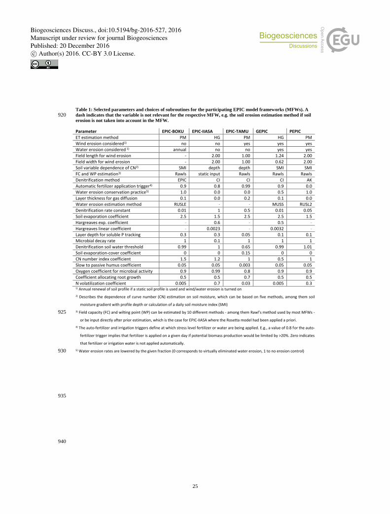
25

Table 1: Selected parameters and choices of subroutines for the participating EPIC model frameworks (MFWs). A

dash indicates that the variable is not relevant for the respective MFW, e.g. the soil erosion estimation method if soil 920 erosion is not taken into account in the MFW.

Parameter EPIC-BOKU EPIC-IIASA EPIC-TAMU GEPIC PEPIC

ET estimation method PM HG PM HG PM

Wind erosion considered1) no no yes yes yes

Water erosion considered 1) annual no no yes yes

Field length for wind erosion - 2.00 1.00 1.24 2.00

Field width for wind erosion - 2.00 1.00 0.62 2.00

Soil variable dependence of CN2) SMI depth depth SMI SMI

FC and WP estimation3) Rawls static input Rawls Rawls Rawls

Denitrification method EPIC CI CI CI AK

Automatic fertilizer application trigger4) 0.9 0.8 0.99 0.9 0.0

Water erosion conservation practice5) 1.0 0.0 0.0 0.5 1.0

Layer thickness for gas diffusion 0.1 0.0 0.2 0.1 0.0

Water erosion estimation method RUSLE - - MUSS RUSL2

Denitrification rate constant 0.01 1 0.5 0.01 0.05

Soil evaporation coefficient 2.5 1.5 2.5 2.5 1.5

Hargreaves exp. coefficient - 0.6 - 0.5 -

Hargreaves linear coefficient - 0.0023 - 0.0032 -

Layer depth for soluble P tracking 0.3 0.3 0.05 0.1 0.1

Microbial decay rate 1 0.1 1 1 1

Denitrification soil water threshold 0.99 1 0.65 0.99 1.01

Soil evaporation-cover coefficient 0 0 0.15 0 0

CN number index coefficient 1.5 1.2 1 0.5 1

Slow to passive humus coefficient 0.05 0.05 0.003 0.05 0.05

Oxygen coefficient for microbial activity 0.9 0.99 0.8 0.9 0.9

Coefficient allocating root growth 0.5 0.5 0.7 0.5 0.5

N volatilization coefficient 0.005 0.7 0.03 0.005 0.3 1) Annual renewal of soil profile if a static soil profile is used and wind/water erosion is turned on

2) Describes the dependence of curve number (CN) estimation on soil moisture, which can be based on five methods, among them soil

moisture gradient with profile depth or calculation of a daily soil moisture index (SMI)

3) Field capacity (FC) and wilting point (WP) can be estimated by 10 different methods - among them Rawl’s method used by most MFWs - 925

or be input directly after prior estimation, which is the case for EPIC-IIASA where the Rosetta model had been applied a priori.

4) The auto-fertilizer and irrigation triggers define at which stress level fertilizer or water are being applied. E.g., a value of 0.8 for the auto-

fertilizer trigger implies that fertilizer is applied on a given day if potential biomass production would be limited by >20%. Zero indicates

that fertilizer or irrigation water is not applied automatically.

5) Water erosion rates are lowered by the given fraction (0 corresponds to virtually eliminated water erosion, 1 to no erosion control) 930

935

940


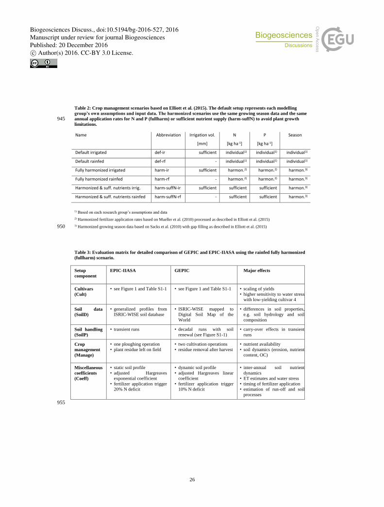
26

Table 2: Crop management scenarios based on Elliott et al. (2015). The default setup represents each modelling

group’s own assumptions and input data. The harmonized scenarios use the same growing season data and the same

annual application rates for N and P (fullharm) or sufficient nutrient supply (harm-suffN) to avoid plant growth 945 limitations.

Name Abbreviation Irrigation vol.

[mm]

N

[kg ha-1]

P

[kg ha-1]

Season

Default irrigated def-ir sufficient individual1) individual1) individual1)

Default rainfed def-rf - individual1) individual1) individual1)

Fully harmonized irrigated harm-ir sufficient harmon.2) harmon.2) harmon.3)

Fully harmonized rainfed harm-rf - harmon.2) harmon.2) harmon.3)

Harmonized & suff. nutrients irrig. harm-suffN-ir sufficient sufficient sufficient harmon.3)

Harmonized & suff. nutrients rainfed harm-suffN-rf - sufficient sufficient harmon.3)

1) Based on each research group’s assumptions and data

2) Harmonized fertilizer application rates based on Mueller et al. (2010) processed as described in Elliott et al. (2015)

3) Harmonized growing season data based on Sacks et al. (2010) with gap filling as described in Elliott et al. (2015) 950

Table 3: Evaluation matrix for detailed comparison of GEPIC and EPIC-IIASA using the rainfed fully harmonized

(fullharm) scenario.

Setup

component EPIC-IIASA GEPIC Major effects

Cultivars

(Cult)

• see Figure 1 and Table S1-1 • see Figure 1 and Table S1-1 • scaling of yields

• higher sensitivity to water stress

with low-yielding cultivar 4

Soil data

(SoilD)

• generalized profiles from

ISRIC-WISE soil database

• ISRIC-WISE mapped to

Digital Soil Map of the

World

• differences in soil properties,

e.g. soil hydrology and soil

composition

Soil handling

(SoilP)

• transient runs • decadal runs with soil

renewal (see Figure S1-1)

• carry-over effects in transient

runs

Crop

management

(Manage)

• one ploughing operation

• plant residue left on field

• two cultivation operations

• residue removal after harvest

• nutrient availability

• soil dynamics (erosion, nutrient

content, OC)

Miscellaneous

coefficients

(Coeff)

• static soil profile

• adjusted Hargreaves

exponential coefficient

• fertilizer application trigger

20% N deficit

• dynamic soil profile

• adjusted Hargreaves linear

coefficient

• fertilizer application trigger

10% N deficit

• inter-annual soil nutrient

dynamics

• ET estimates and water stress

• timing of fertilizer application

• estimation of run-off and soil

processes

955


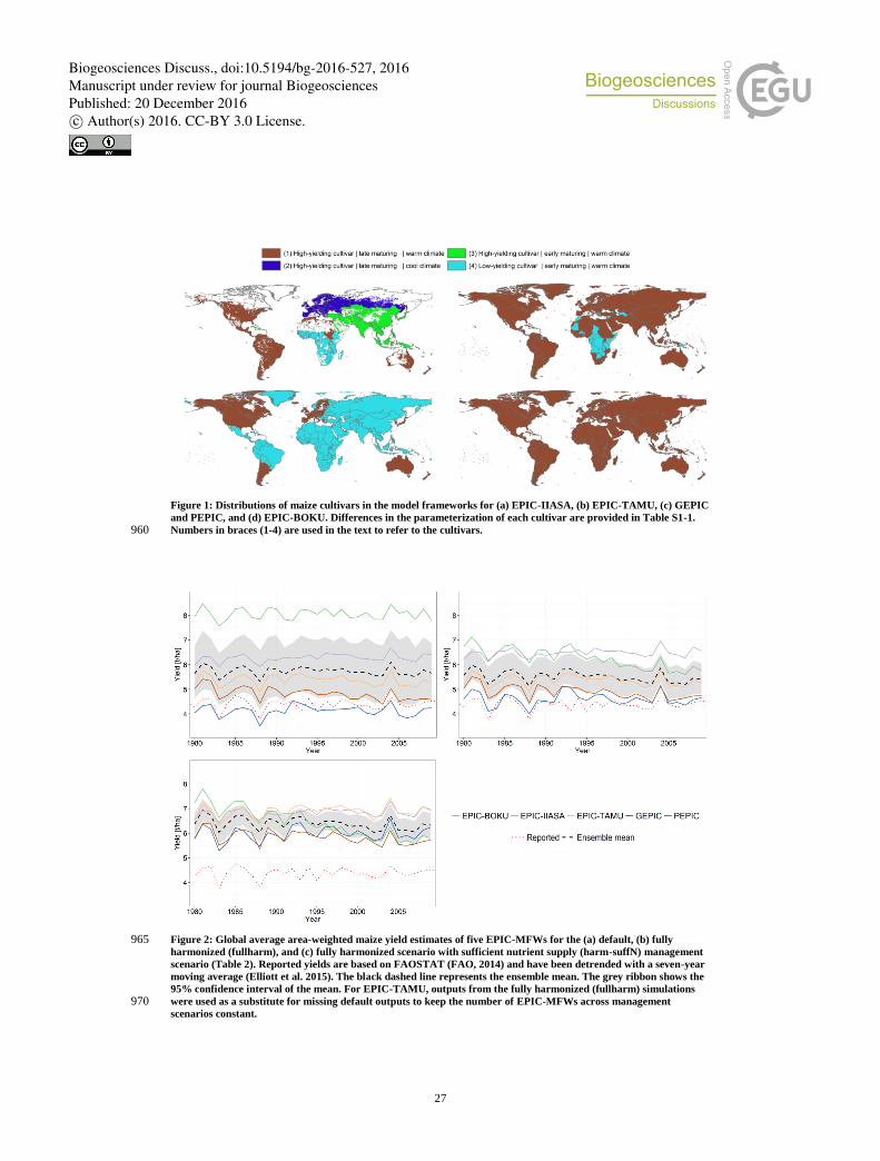
27

Figure 1: Distributions of maize cultivars in the model frameworks for (a) EPIC-IIASA, (b) EPIC-TAMU, (c) GEPIC

and PEPIC, and (d) EPIC-BOKU. Differences in the parameterization of each cultivar are provided in Table S1-1.

Numbers in braces (1-4) are used in the text to refer to the cultivars. 960

Figure 2: Global average area-weighted maize yield estimates of five EPIC-MFWs for the (a) default, (b) fully 965 harmonized (fullharm), and (c) fully harmonized scenario with sufficient nutrient supply (harm-suffN) management

scenario (Table 2). Reported yields are based on FAOSTAT (FAO, 2014) and have been detrended with a seven-year

moving average (Elliott et al. 2015). The black dashed line represents the ensemble mean. The grey ribbon shows the

95% confidence interval of the mean. For EPIC-TAMU, outputs from the fully harmonized (fullharm) simulations

were used as a substitute for missing default outputs to keep the number of EPIC-MFWs across management 970 scenarios constant.


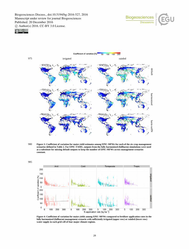
28

975

Figure 3: Coefficient of variation for maize yield estimates among EPIC-MFWs for each of the six crop management 980 scenarios defined in Table 2. For EPIC-TAMU, outputs from the fully harmonized (fullharm) simulations were used

as a substitute for missing default outputs to keep the number of EPIC-MFWs across management scenarios

constant.

985

Figure 4: Coefficient of variation for maize yields among EPIC-MFWs compared to fertilizer application rates in the

fully harmonized (fullharm) management scenario with sufficiently irrigated (upper row) or rainfed (lower row)

water supply in each grid cell of four major climate regions.

defau

lt

rainfed

harm

onized

harm

-suffN

irrigated


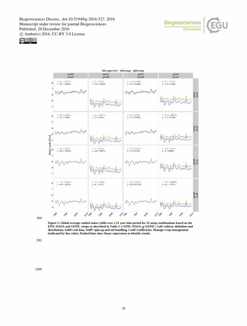
29

990

Figure 5: Global average rainfed maize yields over a 31 year time period for 32 setup combinations based on the

EPIC-IIASA and GEPIC setups as described in Table 3. e=EPIC-IIASA, g=GEPIC, Cult=cultivar definition and

distribution, SoilD=soil data, SoilP=spin-up and soil handling, Coeff=coefficients, Manage=crop management

(indicated by line color). Dashed lines show linear regressions to identify trends.

995

1000


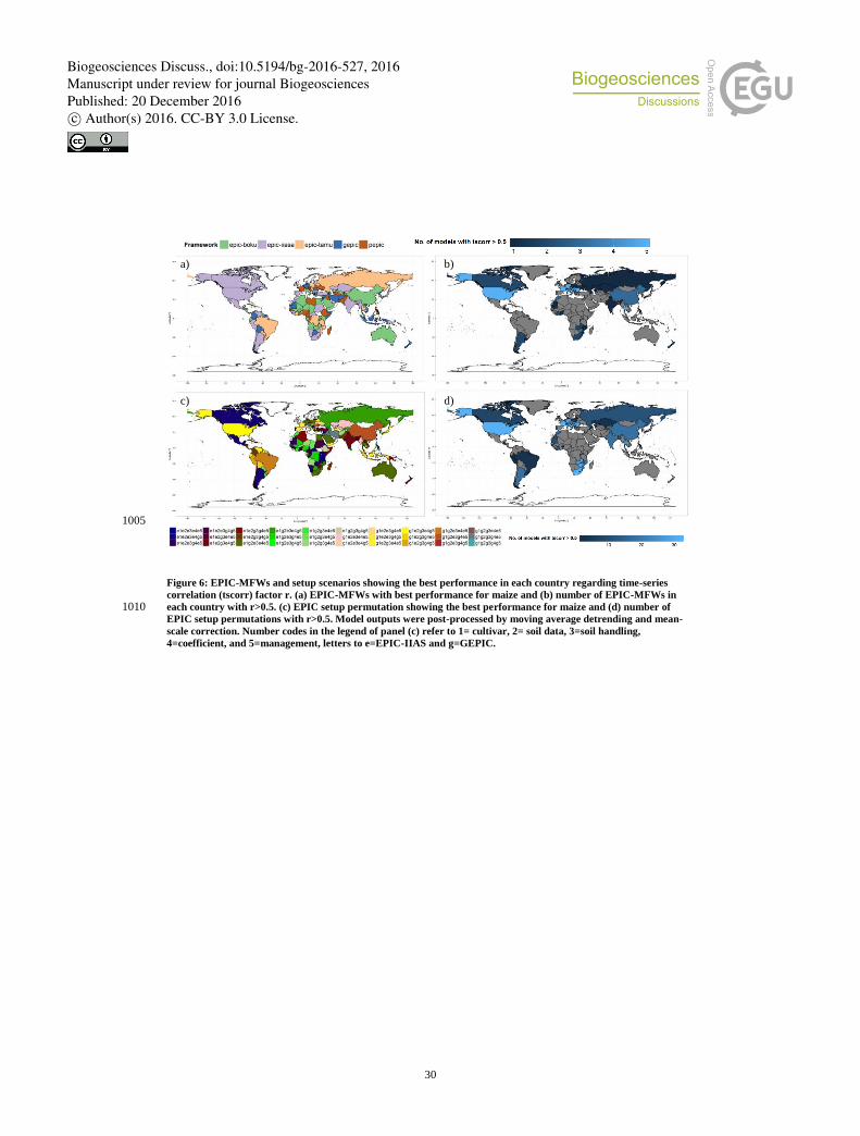
30

1005

Figure 6: EPIC-MFWs and setup scenarios showing the best performance in each country regarding time-series

correlation (tscorr) factor r. (a) EPIC-MFWs with best performance for maize and (b) number of EPIC-MFWs in

each country with r>0.5. (c) EPIC setup permutation showing the best performance for maize and (d) number of 1010 EPIC setup permutations with r>0.5. Model outputs were post-processed by moving average detrending and mean-

scale correction. Number codes in the legend of panel (c) refer to 1= cultivar, 2= soil data, 3=soil handling,

4=coefficient, and 5=management, letters to e=EPIC-IIAS and g=GEPIC.

a) b)

c) d)


uncertainties in global crop model frameworks: effects of ...pure.iiasa.ac.at/14232/1/uncertainties...

Documents