ultrasound imaging system combined with multi...
TRANSCRIPT
ULTRASOUND IMAGING SYSTEM COMBINED WITH MULTI-MODALITY IMAGE
ANALYSIS ALGORITHMS TO MONITOR CHANGES IN ANATOMICAL
STRUCTURES
by
Vikas Revanna Shivaprabhu
B.E., Visveswaraya Technological University, 2008
M.S., University of Pittsburgh, 2010
Submitted to the Graduate Faculty of
Swanson School of Engineering in partial fulfillment
of the requirements for the degree of
Doctor of Philosophy
University of Pittsburgh
2015

UNIVERSITY OF PITTSBURGH
SWANSON SCHOOL OF ENGINEERING
This dissertation was presented
by
Vikas Revanna Shivaprabhu
It was defended on
January 27, 2015
and approved by
Dr. Lance Davidson, Ph.D., Associate Professor, Department of Bioengineering
Dr. Dana Tudorascu, Ph.D., Assistant Professor of Medicine, Biostatistics, Psychiatry and
Clinical and Translational Science
Dissertation Co-Director: George Stetten, MD, Ph.D., Professor, Department of
Bioengineering
Dissertation Co-Director: Howard Aizenstein, MD, Ph.D., Associate Professor, Department of
Psychiatry and Bioengineering
ii

Copyright © by Vikas Revanna Shivaprabhu
2015
iii
ULTRASOUND IMAGING SYSTEM COMBINED WITH MULTI-MODALITY IMAGE
ANALYSIS ALGORITHMS TO MONITOR CHANGES IN ANATOMICAL
STRUCTURES
Vikas Revanna Shivaprabhu, B.E., M.S., Ph.D.
University of Pittsburgh, 2015
This dissertation concerns the development and validation of an ultrasound imaging system and
novel image analysis algorithms applicable to multiple imaging modalities. The ultrasound
imaging system will include a framework for 3D volume reconstruction of freehand ultrasound:
a mechanism to register the 3D volumes across time and subjects, as well as with other imaging
modalities, and a playback mechanism to view image slices concurrently from different
acquisitions that correspond to the same anatomical region. The novel image analysis algorithms
include a noise reduction method that clusters pixels into homogenous patches using a directed
graph of edges between neighboring pixels, a segmentation method that creates a hierarchical
graph structure using statistical analysis and a voting system to determine the similarity between
homogeneous patches given their neighborhood, and finally, a hybrid atlas-based registration
method that makes use of intensity corrections induced at anatomical landmarks to regulate
deformable registration. The combination of the ultrasound imaging system and the image
analysis algorithms will provide the ability to monitor nerve regeneration in patients undergoing
regenerative, repair or transplant strategies in a sequential, non-invasive manner, including
visualization of registered real-time and pre-acquired data, thus enabling preventive and
iv

therapeutic strategies for nerve regeneration in Composite Tissue Allotransplantation (CTA).
The registration algorithm is also applied to MR images of the brain to obtain reliable and
efficient segmentation of the hippocampus, which is a prominent structure in the study of
diseases of the elderly such as vascular dementia, Alzheimer’s, and late life depression.
Experimental results on 2D and 3D images, including simulated and real images, with
illustrations visualizing the intermediate outcomes and the final results are presented.
v

TABLE OF CONTENTS
1.0 INTRODUCTION ........................................................................................................ 1
1.1 THESIS STATEMENT ....................................................................................... 1
1.2 OVERVIEW OF CONTRIBUTIONS ............................................................... 2
1.3 THESIS ORGANIZATION ................................................................................ 3
2.0 BACKGROUND AND SIGNIFICANCE .................................................................. 4
2.1 CLINICAL SIGNIFICANCE ............................................................................. 4
2.1.1 Nerve regeneration .......................................................................................... 4
2.1.2 Alzheimer’s Disease ......................................................................................... 7
2.2 TECHNOLOGY BACKGROUND .................................................................... 8
2.2.1 Ultrasound imaging ......................................................................................... 8
2.2.2 High Resolution Ultrasound (HRUS) .......................................................... 12
2.2.3 Volumetric Ultrasound.................................................................................. 14
2.2.4 Magnetic Resonance Imaging (MRI) ........................................................... 16
2.2.5 Medical Image Analysis ................................................................................ 18
2.2.5.1 Image segmentation ............................................................................ 20
2.2.5.2 Image registration ............................................................................... 26
2.2.5.3 Visualization ........................................................................................ 28
3.0 INNOVATION ........................................................................................................... 30
vi

3.1 MONITOR NERVE REGENERATION ........................................................ 30
3.2 OVERVIEW OF THE DEVELOPED SYSTEM ........................................... 31
3.3 AUTOMATED IMAGE ANALYSIS ............................................................... 33
4.0 FREEHAND 3D RECONSTRUCTION .................................................................. 36
5.0 IMAGE SEGMENTATION ...................................................................................... 44
5.1 SHELLS AND SPHERES ................................................................................. 45
5.2 FEATURE BASED SEGMENTATION .......................................................... 48
5.3 VARIANCE DESCENT GRAPHS .................................................................. 54
5.4 GRAPH BASED TECHNIQUES ..................................................................... 61
5.4.1 Constructing a graph of patches .................................................................. 64
5.4.1.1 Graph notation .................................................................................... 64
5.4.1.2 Voting system....................................................................................... 65
5.4.2 Clustering regions in the graph of patches .................................................. 74
5.4.2.1 Affinity propagation ........................................................................... 75
5.4.2.2 Dominant Sets ...................................................................................... 76
5.4.3 Segmenting anatomical structures ............................................................... 79
5.4.4 Results on Simulated Data ............................................................................ 81
5.4.4.1 Community Distribution .................................................................... 82
5.4.4.2 Rand index ........................................................................................... 84
5.4.4.3 Simulated 3D Image ............................................................................ 85
5.4.5 Results on Real Ultrasound Data ................................................................. 87
5.4.5.1 Ultrasound of phantom ....................................................................... 87
5.4.5.2 Ultrasound nerve image ...................................................................... 88
vii
5.4.5.3 3D reconstructed ultrasound of phantom ......................................... 90
5.4.5.4 3D reconstructed ultrasound of the median nerve ........................... 92
5.4.5.5 Comparison with pairwise similarity measure ................................. 94
6.0 IMAGE REGISTRATION ........................................................................................ 96
6.1 HYBRID LANDMARK-INTENSITY BASED REGISTRATION............... 97
6.1.1 Methodology ................................................................................................... 98
6.1.1.1 Identify Landmarks ............................................................................ 98
6.1.1.2 Landmark Registration ...................................................................... 98
6.1.1.3 Alter the image intensity................................................................... 101
6.1.1.4 Deformable intensity registration .................................................... 102
6.2 VALIDATION ON HIPPOCAMPUS SEGMENTATION ......................... 104
6.2.1 Comparison with previous similar methods ............................................. 105
6.2.2 Quantitative comparison with other methods ........................................... 106
7.0 SIMULTANEOUS VISUALIZATION .................................................................. 109
7.1 REGISTRATION OF PRIOR AND ACQUIRED VOLUMES .................. 110
7.2 OFFLINE SIMULTANEOUS VISUALIZATION ....................................... 111
7.3 REAL-TIME SIMULTANEOUS VISUALIZATION ................................. 112
8.0 DISCUSSION AND FUTURE WORK .................................................................. 118
8.1 FUTURE DIRECTIONS................................................................................. 122
8.1.1 ProbeSight .................................................................................................... 123
BIBLIOGRAPHY ..................................................................................................................... 125
viii

LIST OF TABLES
Table 1 Rand Index computed for four images shown in Figure 30 ............................................ 84
ix

LIST OF FIGURES
Figure 1 Illustration showing Wallerian degeneration (reprinted from (Burnett & Zager, 2004)). 5
Figure 2 Lateral view of the brain highlighting the hippocampus .................................................. 7
Figure 3 Nerve image with individual fascicles scanned using VisualSonics Vevo 2100 system at 50 MHz .......................................................................................................................... 13
Figure 4 HRUS image (Vivo 2100) of artery showing measurement of Intimal Thickness (IT), Intima-Media Thickness (IMT), and Lumen Diameter (LD). ....................................... 13
Figure 5 A) 3D probe with 2D “matrix” array acquiring 3D volumes directly ("3D Imaging Using 2D CMUT Arrays with Integrated Electronics,"). B) 3D probe with an internal 2D probe that is mechanically swept repeatedly in the third dimension. C) Reconstructing a 3D volume from the 2D images based on the position and orientation of a hand-held 2D ultrasound probe............................................................................... 15
Figure 6 Overview of the developed system together with the individual methods that have been developed, and their arrangement in the pipeline. ......................................................... 32
Figure 7 System overview of 3D volume reconstruction ............................................................. 37
Figure 8 The image acquisition system and the tracking system generates data at their own rates......................................................................................................................................... 37
Figure 9 Temporal calibration estimates the latency between the tracking and imaging systems. Location data of the two systems before (top) and after (bottom) compensating for the latency. ........................................................................................................................... 39
Figure 10 A) CAD model of the N-wire phantom. (Lasso et al., 2014). B) 3D printed N-wire phantom with reference marker attached .................................................................... 40
Figure 11 Ultrasound image of the N-wires, which was acquired with the phantom immersed in water bath. The wires appear as dots, as seen in the image at locations pointed by the red arrows.................................................................................................................... 40
Figure 12 3D rendering of the segmentation of the wires from the freehand reconstructed volume of the N-wire phantom. Also shown are three orthogonal slices. .............................. 42
Figure 13 (A) US probe tracked by markers mounted on it. (B) 3D model of individual 2D US images stacked in a 3D space based on the recorded location and orientation of the US probe. (C) Live US image. (D) US image slice retrieved from a previously reconstructed US volume corresponding to the live US image. ................................. 43
x
Figure 14 (A) Asymmetric sphere-pairs (B) Search algorithm to find the nearest boundary of the rectangular area. .......................................................................................................... 45
Figure 15 (A) 3D model of a torus visualized using surface rendering. (B) Noisy image of a torus. Cross-sectional slice of the 3D image showing the detected medial points at scale 5 (blue), and at scale 6 (green). Reproduced from (Revanna Shivaprabhu, 2010)..................................................................................................................................... 48
Figure 16 (B) shows the result of applying the methods mentioned above to a binary segmentation of the hippocampus (A). The medial manifold is represented by cubes in the figure. The color of Eigen vectors represented by arrows positioned at cubes and the color of the cubes indicate the partitions obtained after applying normalized cuts method. ................................................................................................................ 52
Figure 17 Illustrations of cases where the methods described above is likely to fail. (A) The boundary separating the hippocampus and the adjacent amygdala is very thin, as seen at the location of the red arrow. The outer sphere in such cases is likely to encompass more than the neighboring amygdala, leading to erroneous identification of boundary. (B) Missing boundaries such as those that appear in the ultrasound images of the median nerve can result in unpredictable medial manifolds. ...................................... 54
Figure 18 Directed edges (arrows) between pixels (circles) representing decreasing intensity variance of spheres centered on those pixels. Reproduced from (G. Stetten et al., 2013) ........................................................................................................................... 55
Figure 19 Flowchart for the variance descent graphs algorithm................................................... 56
Figure 20 Flowchart for the recursive function ‘Follow tree recursively’ used in the flowchart shown in Figure 19...................................................................................................... 57
Figure 21 Variance descent graph applied at various radii (in pixels) to an ultrasound image of the median nerve. ........................................................................................................ 59
Figure 22 Variance descent graph applied MRI image of the brain. Shown in left is the original image and in right the VDG patches evaluated at radius 1 ......................................... 60
Figure 23 (A) 50 MHz ultrasound image of the median nerve. The boundaries between fascicles are often incomplete, as seen at locations highlighted by red circles. (B) VDG Patches obtained for radius 2. The roots of patches are displayed as black dots. (C) Patches are converted to nodes (roots of patches) and edges of a graph. Figure shows an example of edges incident on one node (position of crosshairs) ........................... 65
Figure 24 Synthetic isotropic image depicting the SAS framework applied to patches. A and B are two distinct patches. Numbers assigned to pixels denotes inter-pixel distance from the central pixel x, denoted 0. The circle denotes sphere Sr(x) where the radius r = 2. .............................................................................................................................. 67
Figure 25 Radius of 𝐒𝐒𝒓𝒓(𝐱𝐱) computed at each node using change in variance method. ............... 69
Figure 26 Spheres of influence (dotted green) obtained for two nodes (crosshairs) along with the subgraph enclosed in each 𝐒𝐒𝒓𝒓(𝐱𝐱) (shown in yellow and blue). Edges belonging to both spheres of influence are shown in red ................................................................. 72
xi
Figure 27 Graph structure generated by asserting each node’s degree of influence on edges in its sphere(s) of influence for the data in Figure 23B. Color of the edge represents its weight (see color bar). Edges with weights equal to 0 are not shown ....................... 74
Figure 28 Clusters obtained for the affinity matrix (A) by applying affinity propagation (B) and dominant sets (C) algorithms. ..................................................................................... 79
Figure 29 Our hierarchical graph structure for segmentation. Starting with pixels, each level is associated with a graph whose nodes are data element resulting from the previous level. ............................................................................................................................ 80
Figure 30 Axial slice of a 3D image consisting of three cylinders representing nerve fascicles with a surrounding sheath, located adjacent to each other such that the boundaries between them are incomplete. Gaussian noise is added to generate images having SNR 5db (A), 10db (B), 15db (C), and 20db (D). ...................................................... 82
Figure 31 Community distribution for the simulated images shown in Figure 30 ....................... 83
Figure 32 (A) Cross section through a simulated 3D image containing tortuous tubular structure. (B) Patches computed at radius 2. Individual colored voxels represent fragments and the labels within the structure are the segmentation results obtained by applying threshold based on expected intensity......................................................................... 85
Figure 33 (A) Graph structure leading to the fragments with a axial image plane of the 3D volume of patches. The 3D model of fragments in (B) is also shown in green. Edges of the graph with low weights have been omitted for illustrative purposes. The color of the edges represents weights (refer color bar). (B) 3D model depicting the fragments..................................................................................................................... 86
Figure 34 Patches generated at radius 14(B) for the ultrasound image of a gel phantom (A). ..... 87
Figure 35 Graph structure associated with the first level communities overlaid on patches (A). Second level communities (clusters of fragments) obtained using affinity propagation (B) and dominant sets (C) ........................................................................................... 88
Figure 36 Individual fascicles identified by clustering fragments using affinity propagation (A & B) and dominant sets (C & D) algorithms. The inherent nature of our method to find spherical structures helps define boundaries between fascicles ................................. 89
Figure 37 (A) Freehand 3D reconstructed ultrasound volume of a gel phantom. (B) Patches computed at radius 1. Colored voxels represents fragments. Also the segmentation obtained by applying a threshold based on expected intensity is shown. ................... 90
Figure 38 (A) Graph structure leading to the fragments with a coronal image plane of the 3D volume of patches. The 3D model of the segmentation in (B) is also shown in green. Edges of the graph with low weights have been omitted for illustrative purposes. The color of the edges represents weights (refer color bar). (B) 3D model of the segmentation. .............................................................................................................. 91
Figure 39 Cross-sectional view of patches computed at radius 3. Colored voxels represents fragments. Also the segmentation obtained by applying a threshold based on expected intensity is shown. ....................................................................................... 92
xii

Figure 40 (A) Graph structure leading to the fragments with an axial image plane of the 3D volume of patches for freehand 3D reconstructed ultrasound volume of the median nerve. Edges of the graph with low weights have been omitted for illustrative purposes. The color of the edges represents weights (refer color bar). (B) Segmentation result overlaid on the original image. .................................................. 93
Figure 41 3D model of the segmentation result with a cross-sectional image plane. .................. 94
Figure 42 Affinity propagation (A) and Dominant sets (B) algorithms applied to a graph structure modeled by pairwise similarity measures. An expected intensity threshold has been applied to obtain the final result.................................................................................. 95
Figure 43 Pipeline of the hybrid registration method ................................................................... 97
Figure 44 (1-4) Sagittal view of MR image of brain showing the positioning of six landmarks (A-F). (5) 3D view showing the six landmarks with axial and sagittal slices in the background .................................................................................................................. 98
Figure 45 (1) 3D view of landmarks positioned in atlas (A~ - F~) and subject (A – F) with axial and sagittal slices. (2) Grid of the resulting affine transform (3) Landmarks in the atlas warped by affine transform ................................................................................. 99
Figure 46 (1) Deformation field obtained from non-linear landmark registration to be applied to the landmarks A~ - F~ (2) 3D view of landmarks showing excellent correspondence after they are warped by the deformation field ......................................................... 101
Figure 47 Image slices corresponding to the landmarks A~ - F~ (highlighted by red circles) after applying Ƒ(A*). Notice the change in image intensity at the location of landmarks 102
Figure 48 Deformation field obtained from demons warp for slice corresponding to landmarks E~ and F~ shown in Figure 46 ................................................................................. 104
Figure 49 Overlap measures for each subject using the method described in this paper in comparison to previously reported results in (Carmichael et al., 2005) ................... 106
Figure 50 Cross-sectional sagittal views of the segmentation results of FreeSurfer (row A), FIRST (row B), our method (row C), and manual segmentation (row D). The false positives, indicated by red circles, are significantly higher in both FIRST and FreeSurfer. ................................................................................................................ 107
Figure 51 Volumes in the standard space are loaded and linked in 3D Slicer, such that moving through image slices in one volume will automatically display corresponding image slices from the other volumes ................................................................................... 112
Figure 52 Rendered CT image of a gel phantom embedded with vascular structures that is MR/Ultrasound compatible ....................................................................................... 113
Figure 53 Three orthogonal views of an MR image of the phantom shown in Figure 52 .......... 114
Figure 54 Cross-sectional view of the reconstructed ultrasound volume overlaid on the registered MR image.................................................................................................................. 115
Figure 55 3D Slicer interface for the real-time simultaneous visualization. Top left: Slices extracted from MR image overlaid on a reconstructed ultrasound volume corresponding to the current position and orientation of the ultrasound probe. Bottom
xiii

left: Live ultrasound image transmitted from the scanner. Bottom right: Slice of MR image. Top right: 3D rendering of segmentation of vascular structure together with images seen in top left and bottom right windows. .................................................. 116
xiv

1.0 INTRODUCTION
1.1 THESIS STATEMENT
Development and validation of an ultrasound imaging system and image analysis methodologies,
including a framework for 3D volume reconstruction of freehand ultrasound, a playback
mechanism to view image slices concurrently from different acquisitions that correspond to the
same anatomical region, a multi-modality hybrid image registration method, and an automated
robust image segmentation method will enhance the ability to monitor changes, study
functionality and analyze geometry of anatomical structures.
1

1.2 OVERVIEW OF CONTRIBUTIONS
i. A system to acquire freehand 3D reconstructed ultrasound images has been implemented.
ii. A technique to concurrently visualize, in real-time, multiple reconstructed volumes including
3D ultrasound and other imaging modalities has been developed.
iii. A hybrid atlas based registration method that makes use of intensity corrections induced at
anatomical landmarks to regulate deformable intensity registration has been developed. The
method is evaluated on the task of segmentation of the hippocampus in MR images of the
brain.
iv. An n-dimensional image analysis method for clustering pixels into homogeneous regions
using a directed graph of edges between neighboring pixels has been developed.
v. An n-dimensional automated method that makes use of statistical analysis and graph theory
to segment individual fascicles in ultrasound images of the median nerve has been developed.
2
1.3 THESIS ORGANIZATION
The clinical significance of the systems and methods that have been developed are described in
section 2.1. Specifically, the mechanism of nerve regeneration and its significance in patients
with peripheral nerve injury is described in section 2.1.1, and the hippocampus and its role in
diseases of the elderly such as Alzheimer’s disease (AD) is described in section 2.1.2. The
technologies related to the topics covered in this dissertation are introduced in section 2.2,
including, ultrasound imaging (section 2.2.1), high resolution ultrasound (section 2.2.2),
volumetric ultrasound (section 2.2.3), magnetic resonance imaging (section 2.2.4), and various
topics in medical imaging analysis (section 2.2.5), such as image segmentation (section 2.2.5.1),
image registration (section 2.2.5.2), and visualization (section 2.2.5.3). The innovation presented
in this dissertation is summarized in section 3.0. In section 3.2, an overview of the developed
system is illustrated. The novel image analysis methods that have been developed are
summarized in section 3.3. The freehand 3D reconstruction system that has been implemented is
described in section 4.0. In section 5.0 , the developed image segmentation methods are
presented. A previously developed medial detection framework is reviewed in section 5.1. A
method to transform medial features to a graph structure in feature space, and generate
segmentation is explored in section 5.2. A method for clustering pixels into homogeneous
regions using a directed graph of edges between neighboring pixels is described in section 5.3.
A method that makes use of statistical analysis and graph theory to segment individual fascicles
in ultrasound images of the median nerve is described in section 5.4. The hybrid registration
method, together with the validation of the method is reported in section 6.0 . A technique to
concurrently visualize multiple 3D volumes, both in offline and real-time mode, is described in
section 7.0 . Discussion and future work can be found in Section 8.0
3

2.0 BACKGROUND AND SIGNIFICANCE
In this section, the clinical significance of the methods developed as part of this dissertation is
discussed in section 2.1. The technologies related to the methods are introduced in section 2.2.
2.1 CLINICAL SIGNIFICANCE
The ultrasound imaging system and the n-dimensional segmentation algorithm developed as part
of this dissertation are general medical imaging advances that can potentially enhance the ability
to monitor changes, study functionality and analyze geometry of anatomical structures across
disorders. Two particular current clinical dilemmas motivated this work: monitoring nerve
regeneration in composite tissue allotransplantation (CTA) and hippocampal segmentation from
high-resolution MRI in individuals with Alzheimer’s disease.
2.1.1 Nerve regeneration
Composite tissue allotransplantation (CTA) involves the transplantation of multiple tissues
including skin, muscle, tendon, bone, cartilage, fat, nerves and blood vessels, unlike
conventional solid organ transplantation, which involves single separate organ. CTA mainly
focuses on improving the quality of life by restoring anatomic, cosmetic, and functional integrity.
4
Hand transplantation is a form of composite tissue allotransplantation, whereby the hand of a
cadaveric donor is transferred to the forearm of an amputee. The first successful hand
transplants were performed in 1998–99 by teams in Lyon (France), Louisville (KY), and
Guangzhou (China) (Barker, Francois, Frank, & Maldonado, 2002). By 2013, the International
Registry on Hand and Composite Tissue Transplantation (IRHCTT) had received details of 51
hand transplants with encouraging outcomes ("Hand Registry,"). The focus of current CTA
research/clinical trials is to improve the safety, efficacy and applicability of these promising
reconstructive modalities. Nerve Regeneration is a major challenge that affect the outcome of
these life-enhancing procedures.
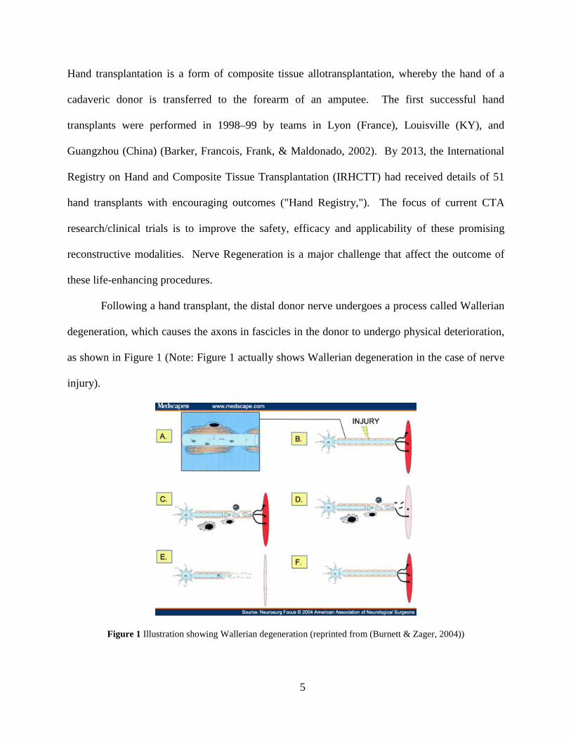
Following a hand transplant, the distal donor nerve undergoes a process called Wallerian
degeneration, which causes the axons in fascicles in the donor to undergo physical deterioration,
as shown in Figure 1 (Note: Figure 1 actually shows Wallerian degeneration in the case of nerve
injury).
Figure 1 Illustration showing Wallerian degeneration (reprinted from (Burnett & Zager, 2004))
5

The axons and surrounding myelin in the donor hand break down (B to D in Figure 1).
As the degradation of the distal nerve segment continues, connection with the target muscle is
lost, leading to muscle atrophy (Burnett & Zager, 2004) (E in Figure 1). Distal muscles that have
lost their innervation have impaired/no function and will undergo atrophy if new axons do not
reach the motor end plates in time. At this stage, only the nerve sheaths/tubes remain in the
donor hand to serve as conduits.
Axons grow from the recipient, advancing towards the donor target muscles. Once
reinnervation is complete, the axons mature and the pre-injury cytoarchitecture and function are
restored. In addition to hand-transplants, nerve regeneration also takes place in peripheral nerve
injury (PNI), which is a serious health problem, with approximately 360,000 people in the
United States suffering from upper extremity paralytic syndromes yearly and affecting 2.8% of
trauma patients (Kesley, Praemer, Nelson, Felberg, & Rice, 1997). In addition to civilian causes
(motor vehicle accidents, lacerations with sharp objects, penetrating trauma, stretching or
crushing trauma and fractures, and gunshot wounds), devastating PNI is also seen in war injuries,
due primarily to improvised explosive device (IED) blast trauma from shrapnel of various
dimensions, shapes, and velocities..
The ability to objectively diagnose nerve injury or monitor nerve regeneration in patients
undergoing regenerative, repair, or transplant strategies (recipients of CTA such as hand
transplants or after PNI treatments such as nerve repair) in a sequential, inexpensive, non-
invasive manner would be a significant improvement in the treatment of these patients and study
of the underlying processes.
6

2.1.2 Alzheimer’s Disease
Alterations of hippocampal activity play a vital role in conditions such as Alzheimer’s disease
(AD), schizophrenia, and epilepsy. In 2013, approximately 5.2 million people had AD in the
U.S. alone, and it is the sixth leading cause of death (Thies & Bleiler, 2013). The hippocampus
is a paired structure that belongs to the limbic system. It has mirror-image halves in the left and
right sides of the brain and a distinct curved shape (see Figure 2). The hippocampus is located
inside the medial temporal lobe, beneath the cortical surface, and consists of ventral and dorsal
portions. It is involved in a variety of cognitive and emotional functions, including long-term
memory, olfaction, and spatial navigation.
Figure 2 Lateral view of the brain highlighting the hippocampus
In AD, the hippocampus is one of the regions that are primarily affected. Studies indicate
that AD patients have significantly smaller volumes of both hippocampi and the left frontal lobe
(Laakso et al., 1995). There appears to be a reduction in the size of hippocampus in patients as
they progress from mild cognitive impairment to AD. Recent developments in Magnetic
Resonance Imaging (MRI) have resulted in high-resolution images of the brain, making it
possible to identify various structures in high detail. Hence, it is of utmost importance for both
basic neuroscience and clinical research that reliable and efficient methods for accurately
7

segmenting the hippocampus in MR images of the brain are developed. Such methods would
further aid in studying the function and structure of the hippocampus in the living human brain as
it relates to various other conditions.
2.2 TECHNOLOGY BACKGROUND
2.2.1 Ultrasound imaging
Ultrasound imaging makes use of backscattering phenomenon of acoustic signals with
frequencies in the MHz range (too high for humans to hear) to generate images of the internal
anatomy including tendons, muscles, joints, vessels and internal organs for diagnostic purposes.
Typically, piezoelectric transducers encased in a casing and driven by electric pulses are used to
generate acoustic signals at the desired frequency. Ultrasound beams are focused either by
physical lenses or by using phased array techniques (beamforming). The sound waves travel into
the target structure, being partially reflected from the layers between different tissues or scattered
by very small structures. A certain fraction of the reflected sound waves (echo) return to the
same transducers that generated the initial signal, which now act as receivers and convert the
backscattered waves to electric pulses, which, after amplification and filtering are processed into
images. Depending on the time it took for the sound wave to propagate through the medium and
reflect back to the source, as well as the intensity of the reflected signal, the ultrasound machine
determines the intensity of the pixels at specific locations in the image.
The strength of the echo depends on the change of acoustical impedance in the material
that generates the echo. The change in acoustical impedance is so high between air and any
8
other substance that virtually all the ultrasound waves are reflected where air is encountered in
the beam path. Hence, ultrasound imaging requires a point of contact with no air present
between the transducer and the patient. Since ultrasound waves travel easily through liquids, a
thick liquid (gel) is commonly used to bridge the gap.
Ultrasound scanners typically operate at frequencies between 1 and 20 MHz. The spatial
resolution, which defines the distance between two scatterers at which they are resolvable, is
inversely proportional to frequency. In other words, the axial resolution improves (the
resolvable distance decreases) with increasing frequency. The attenuation of the ultrasound
beam as it propagates through the target structure is also strongly dependent on frequency. The
relationship between attenuation coefficient (in dB cm-1) and frequency (Hz) is approximately
linear (Webb & Kagadis, 2003). For soft tissue, the typical attenuation coefficient is
1 dB cm−1MHz−1. Hence, a trade-off exists between frequency and depth of penetration –
higher frequency results in lower penetration. For this reason, lower frequencies of 1 – 6 MHz
are used to study deep structures such as liver and kidney, while higher frequencies of 7 – 20
MHz, which provide better spatial resolution, are used to study more superficial structures such
as muscles, tendons, nerves and breast.
Transducer arrays are manufactured in varying configurations of piezoelectric crystal
elements to suit different applications. Linear sequential arrays consist of elements that are
arranged in a linear form in which they fire sequentially. The images generated form a
rectilinear grid. These transducers are mostly used for vascular imaging since the flat probe tip
can be oriented to image the longer dimension of the vessels. The transducer elements can also
be arranged into a curved array to acquire a sector image. This arrangement provides a wider
field of view, and is thereby better suited for abdominal imaging, where target structures are
9
larger. Another configuration, known as a phased array also has a linear arrangement of
elements, but unlike linear sequential arrays, uses smaller form factor. The voltage pulses
exciting each element of phased array are delayed with respect to each other to effect beam-
stearing and thus generating a sector image with sequential interrogations. The small form factor
suits cardiovascular applications where the probe is placed in tight windows between the ribs to
image the heart.
A number of different imaging modes are available in ultrasound imaging:
• A-mode: Amplitude (A) mode is a one-dimensional scan, where the amplitude of the
backscattered wave is plotted against the time after transmission of the ultrasound pulse.
• B-mode: Brightness (B) mode results in a two-dimensional image. Each line of the
resulting image consists of an A-mode scan with the amplitude of the backscattered wave
represented as the brightness of the pixel.
• M-mode: Motion (M) mode is a continuous series of A-mode scans that are brightness
modulated and each displayed vertically, while sweeping horizontally for successive
scans. This mode is used to study time-varying displacements of tissues/organs along a
single path and does not encompass a cross-section of the anatomy.
• Color Doppler: This mode uses the Doppler effect caused by moving objects. It is
commonly used to study blood flow, where velocity of blood flow is color coded and
overlaid on the B-mode image.
In this dissertation, only B-mode scans are employed.
The signal-to-noise ratio in ultrasound images is one of the poorest found in all medical
imaging. There are three sources of noise in ultrasound imaging (Webb & Kagadis, 2003). The
first is the noise induced by the electronics of the detection system. The second, known as
10
speckle, is an interference pattern caused by the superposition of the echoes arriving with
random phases and amplitudes from a given resolution cell. The range of speckle is between a
minimum of zero to a maximum that depends on the extent that the interference is destructive or
constructive. Speckle makes the images appear granular although the tissue being imaged is a
grossly homogenous. The third source of noise results from artifacts in the image such as
mirroring, shadowing, posterior enhancement, refraction, side lobes, grating lobes, and
reverberation. A detailed study on artifacts in ultrasound imaging can be found in (Kremkau &
Taylor, 1986).
Ultrasound has many advantages over other imaging modalities. It is non-ionizing and
has no known long term side effects, making it ideal for longitudinal studies where a particular
anatomy needs to be imaged repeatedly over a period of time. It is widely available, being
relatively inexpensive compared to other imaging modalities. Ultrasound scanners are highly
portable making scans easy to perform at the bedside or outside the hospital setting. Ultrasound
scanners can be engineered in a wide range of physical sizes and shapes, including pocket size
scanners, transrectal probes, and intravascular systems. One of the most important advantages of
ultrasound is that it is real time. The operator can visualize anatomy live and dynamically
choose the most informative scan location for a given diagnose. The real time nature also makes
it suitable for image guided interventions such as biopsies, spinal taps, and placement of central
line.
Limitations of ultrasound imaging include low signal-to-noise ratio, which renders
automated image analysis extremely challenging. It requires expert skill, training, and
knowledge of the anatomy to acquire useful ultrasound images. Both location and orientation of
the probe during scanning plays a critical role in the acquisition of images of the desired
11
anatomy. The user should be well versed with ultrasound imaging technology and the effect of
various hardware settings including gain, frequency, focus, and time gain compensation (TGC)
on the resulting images. In addition to the above-mentioned trade-off between resolution and
depth of penetration, the need to maintain contact with the patient makes it difficult to get good
images when imaging at locations with high curvature using a linear probe. Since ultrasound
does not pass through bone or lung, probe location and orientation becomes critical when
imaging targets behind these tissues. In addition, once the images are acquired, the exact
location from which they were acquired is lost, and thus it is difficult to replicate a scan precisely
at a later time.
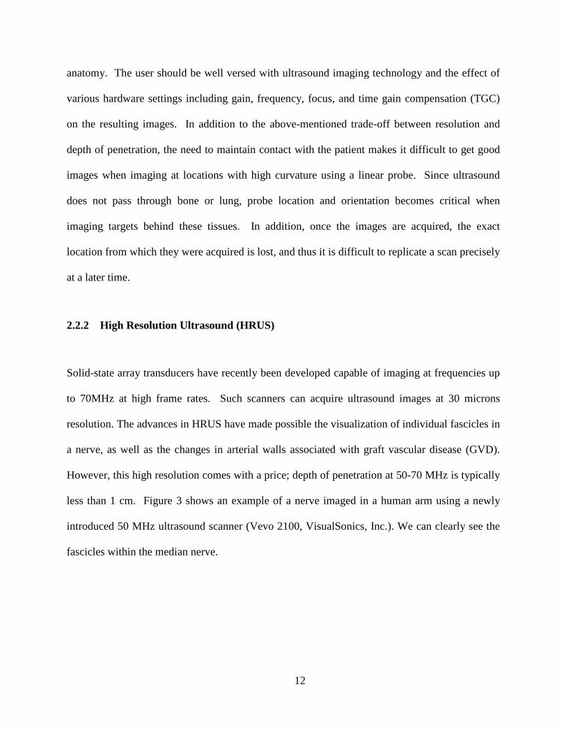
2.2.2 High Resolution Ultrasound (HRUS)
Solid-state array transducers have recently been developed capable of imaging at frequencies up
to 70MHz at high frame rates. Such scanners can acquire ultrasound images at 30 microns
resolution. The advances in HRUS have made possible the visualization of individual fascicles in
a nerve, as well as the changes in arterial walls associated with graft vascular disease (GVD).
However, this high resolution comes with a price; depth of penetration at 50-70 MHz is typically
less than 1 cm. Figure 3 shows an example of a nerve imaged in a human arm using a newly
introduced 50 MHz ultrasound scanner (Vevo 2100, VisualSonics, Inc.). We can clearly see the
fascicles within the median nerve.
12
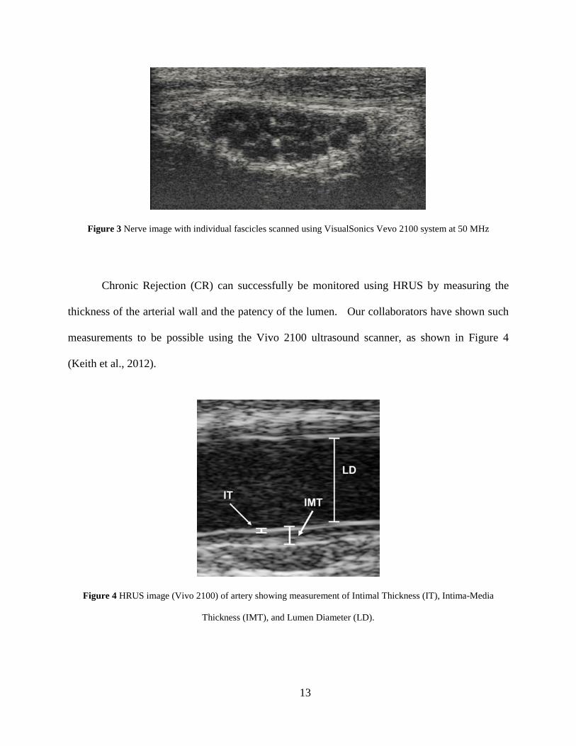
Figure 3 Nerve image with individual fascicles scanned using VisualSonics Vevo 2100 system at 50 MHz
Chronic Rejection (CR) can successfully be monitored using HRUS by measuring the
thickness of the arterial wall and the patency of the lumen. Our collaborators have shown such
measurements to be possible using the Vivo 2100 ultrasound scanner, as shown in Figure 4
(Keith et al., 2012).
Figure 4 HRUS image (Vivo 2100) of artery showing measurement of Intimal Thickness (IT), Intima-Media
Thickness (IMT), and Lumen Diameter (LD).
13
The hand transplant program at UPMC is one of 2 programs using HRUS to monitor CR
changes in their patients (Kaufman et al., 2012). The program has performed one of the largest
number of hand/forearm transplants in the nation (8 transplants in 5 patients). Early evidence
suggests that both arteries and veins may be primary targets of CR in the hand. Although the
UPMC experience confirms that HRUS is a useful tool to evaluate Intimal Hyperplasia (IH) in
vessels, a serious limitation remains in the local 2D nature of the current HRUS technology.
After the scan is completed, the exact anatomical location of the scan at each moment in time is
lost. If the site/location of scan is not registered to a 3D coordinate system, the vascular data
cannot provide an accurate progression for IH in the imaged vessel over time.
2.2.3 Volumetric Ultrasound
Conventional 2D ultrasound has been widely used in medical practice since the 1970’s as a
diagnostic imaging technique to visualize anatomical structures and functions. Lately, 3D
ultrasound is gaining importance because of the additional information it provides for diagnosis
compared to conventional 2D ultrasound. 3D volumes allow direct visualization of anatomy in
3D rendered views. 2D slices can be generated from the 3D volume at arbitrary orientations.
Quantitative measures such as the volume of a structure or particular linear distances within it
may be obtained more accurately given a 3D data set. There are well established image analysis
methods such as registration, segmentation, visualization and volume estimation that work on 3D
images.
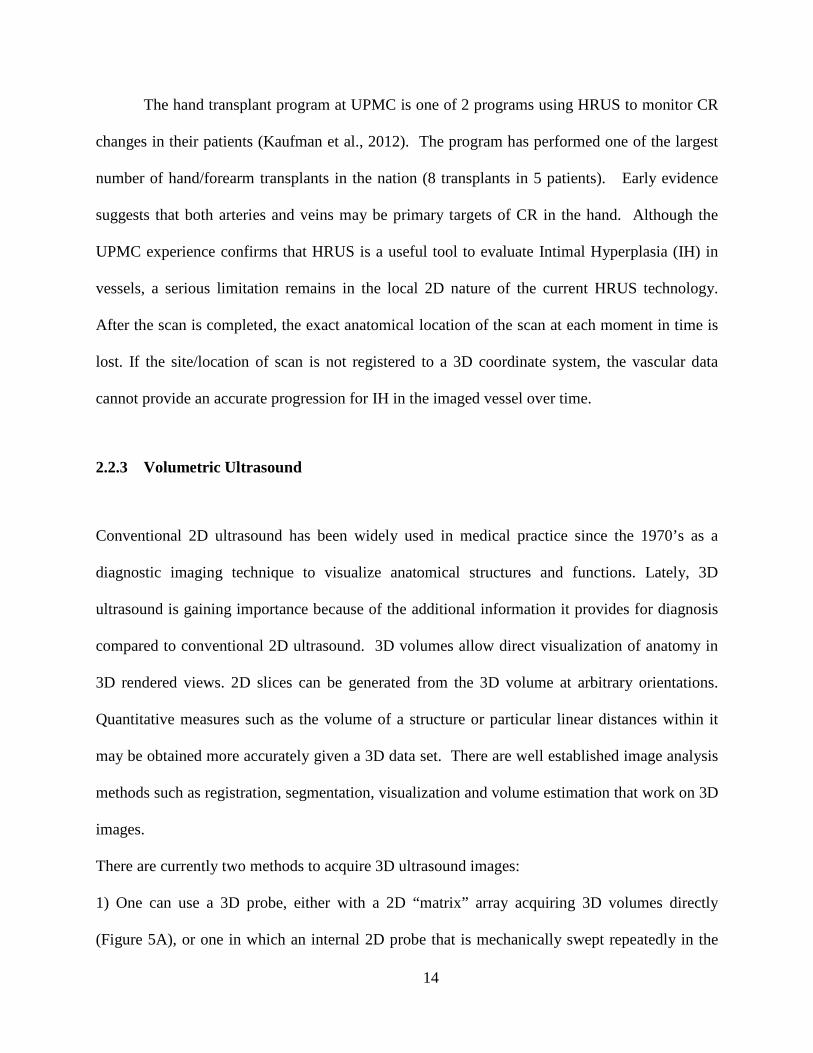
There are currently two methods to acquire 3D ultrasound images:
1) One can use a 3D probe, either with a 2D “matrix” array acquiring 3D volumes directly
(Figure 5A), or one in which an internal 2D probe that is mechanically swept repeatedly in the
14

third dimension (a “wobbler”) (Figure 5B). Matrix array scanners suffer from poor resolution,
and both wobblers and matrix array scanners produce volumes of only a relatively small region
of anatomy at a given time.
2) One can combine slices acquired while manually moving a 2D probe across the patient to
construct a 3D volume (Figure 5C).
Figure 5 A) 3D probe with 2D “matrix” array acquiring 3D volumes directly ("3D Imaging Using 2D CMUT
Arrays with Integrated Electronics,"). B) 3D probe with an internal 2D probe that is mechanically swept repeatedly
in the third dimension. C) Reconstructing a 3D volume from the 2D images based on the position and orientation of
a hand-held 2D ultrasound probe
This second method involves reconstructing a 3D volume from the 2D images based on the
position and orientation of a hand-held 2D ultrasound probe. The probe’s position and
orientation is tracked as it is maneuvered freely without any mechanical restrictions on linear, tilt
and rotational movements. This method has the advantage of covering a much larger region than
the method in (1), while permitting optimal image quality to be maintained by the human
operator manipulating the probe appropriately. Although 3D volume reconstruction
A B C
15
methodologies for hand-held ultrasound have been studied extensively in the past decade
(Estépar et al., 2003; Hsu, Prager, Gee, & Treece, 2008; Rohling, Gee, & Berman, 1999;
François Rousseau, Hellier, & Barillot, 2005), we extend the concept to produce a convenient
and effective visualization tool capable of building 3D US volumes in a standard space, from
acquisitions obtained at different times, for the purpose of monitoring changes in anatomical
structures.
2.2.4 Magnetic Resonance Imaging (MRI)
MR imaging is commonly used to image soft tissues and is based on perturbations of nucleic
magnetic fields using radio waves. Hydrogen nuclei, which are abundantly present in soft tissue
(water and fat molecules) posses strong magnetic moment due to the inherit property of spin
angular momentum. Hence, they are an excellent source of signal to image soft tissue. Although
the orientation of spins of a group of nuclei in a given location of the body is random, thus
producing no net magnetic moment (they cancel each other), the spins can be forced to align by
the application of an external magnetic field (B0). Under the influence of B0, a net magnetic
moment in the same direction as B0 is created. The net magnetic moment can be pushed from
their alignment with B0 by application of radiofrequency (RF) pulses at a specific frequency,
known as the Larmor frequency. This resonant frequency depends on the strength of B0; higher
strength B0 results in higher Larmor frequency. By controlling the strength and duration of the
RF pulse the magnetic moment may be tilted by any desired angle (0o to 180o). When the RF
pulse is done, the spins slowly return to their alignment with B0 while precessing at the Larmor
frequency. This precession induces an AC current in a receive antenna, which is often the same
as that used to apply the RF pulses. The induced AC current forms the signal that is mapped as
16

intensity onto the image. The dependency of the Larmor frequency on the external magnetic
field B0 is exploited by the introduction of gradients in B0 to achieve spatial separation of the
detected signal. Additional magnetic fields, known as x-, y- or z- gradient magnetic fields,
depending on the direction of increasing field strength, cause the resonant frequency for
molecules in the now non-uniform magnetic field to be dependendent on the location of the
molecules within the gradient. Slice selection can be achieved by applying an RF pulse at a
frequency that corresponds to the resonant frequency for a particular area in the gradient field,
leading to the excitation of only those protons in the selected area and the consequent production
of signal from only those protons. Gradients can be generated in arbitrary directions, thereby
making it possible to acquire image planes in arbitrary orientations. To localize protons within a
slice, techniques such as frequency encoding and phase encoding, which make use of Fourier
analysis, are employed. The tissue composition dictates the characteristics of the emitted signal,
with differences in signal strength creating contrast between various tissues in the reconstructed
image. Different aspects of the resonance signal – proton density ρ, spin-lattice relaxation time
T1, and spin-spin relaxation time T2 – can be emphasized by using different MR pulse sequences.
More detailed coverage on MR principles and techniques can be found in (Liang & Lauterbur,
2000).
The main advantages of MR imaging include its non-ionizing nature, high spatial
resolution, flexibility, and high soft tissue contrast. Since, unlike CT, MRI does not involve
exposure to radiation, MRI scans can be safely used for such patients as pregnant women and
infants. A number of imaging sequences of the same patient can be acquired in a single sitting
by varying the RF pulse sequence, each resulting in varying contrast across different tissues.
17

Due to its ability to differentiate soft tissue, MRI can be used to image a wide variety of
structures such as muscles, ligaments, cartilage, brain, heart, liver, eyes, etc.
There are a few drawbacks associated with MR imaging. It is very expensive, mostly
because of the high cost associated with the manufacture of superconducting magnets. A single
MR scanner can cost millions of dollars. Some patients can experience claustrophobia when
they are put in the narrow hole of the scanner, which may be intensified because of the loud
noise emitted by the gradient coils during the scan. Due to the strong magnetic field, patients
with any embedded ferromagnetic metal such as found in pacemakers or shrapnel cannot
undergo MR scans. Furthermore, MR images are susceptible to movement. A single MR scan
can take a long time (greater than 20 minutes), during which time it can be very challenging for
some patients to hold still.
2.2.5 Medical Image Analysis
Medical images produced by a wide range of modalities including the ones described above
provide vital information necessary for diagnosis and treatment. Doctors rely on these images to
predict, diagnose and treat various conditions of the human body. Radiologists and physicians
manually interpret the images using their expert knowledge and training to identify, measure and
functionally assess the structures of the body affected by the conditions under investigation.
This manual process is tedious and time consuming, especially with large 3D datasets such as
those produced by MRI and volumetric ultrasound, which are generally examined one slice at a
time. In addition, the manual analysis of the images is subjective in nature and prone to inter-
subject variability, thus resulting in inconsistencies in the prediction, diagnosis or treatment.
18
Hence, Computer Assisted Image Analysis (CAIA) as a means to assist doctors to extract
information with little or no manual intervention is of critical importance.
CAIA can be applied in a wide variety of clinical scenarios. It can be effective in clinical
research studies where the goal is to understand or confirm findings based on large datasets of
images. Analysis of datasets comprised of thousands of images benefits in great measure if
manual intervention is minimized. The accuracy and reliability of the algorithms used in such
scenarios must be very high since validation of the analysis on each image by a user is not
feasible. Since time constraints on the execution of the algorithms are not critical, the analysis
may be performed offline. CAIA is also used in diagnostics where decisions are made using a
single image or series of images from a single patient, or to guide treatment and study response
to treatment. In these scenarios, manual intervention is acceptable - an expert user provides
initialization to the algorithm or guides the algorithms until convergence. The analyses in these
scenarios may also be performed offline, although, unlike in clinical research studies, the results
should be delivered in a timely manner. Image guided surgery, as the name suggests, makes use
of CAIA to aid the physician to perform surgery. Preoperative images, usually CT and MR, are
used for surgical planning. Reliable image correspondence across modalities and accurate
identification of target structures is critical. Intraoperative images are registered to preoperative
images (and the information extracted from them) by algorithms that execute in real time to
assist in guidance of the surgical procedure. The algorithm can be dependent on user interaction
in the preoperative stage, but should be fully automatic during surgery. CAIA can also be used
for disease prognostics, where the presence/absence of certain bio-markers detected in the
images can predict the chances of a patient developing a certain disease.
19
The most common tasks in CAIA are image segmentation and image registration. Image
segmentation produces delineation of structures in the image. Image registration finds the
transformation that maps one image to another image, such that, the correspondence (intensity or
feature based) of anatomical structures between the two images is maximized. These topics will
be discussed more in detail in the following sections.
2.2.5.1 Image segmentation
Image segmentation is the process of generating delineations in the image based on certain image
attributes. The delineations divide the image into regions such that each region is comprised of
similar attributes. Among others, intensity of the pixels, edges, and texture are some of the most
widely used image attributes. Over the past few decades many novel image segmentation
methods have been developed based on concepts borrowed from mathematics, physics, statistics,
numerical analysis, combinatorial optimization, graph theory, etc., often focused on a specific
application. As such, there does not exist a single method that works in all scenarios for all
applications. In this section, several image segmentation methods are introduced. It is beyond
the scope of this dissertation to perform an exhaustive review of all the segmentation methods or
describe all the details of the algorithms mentioned below. Surveys and in-depth coverage of
these algorithms can be found in (Balafar, Ramli, Saripan, & Mashohor, 2010; Jain, 1989; Noble
& Boukerroui, 2006; Petrou & Petrou, 2010; Pratt, 1991; Toennies, 2012; Yoo, 2004).
Segmentation methods can be broadly classified into three categories: manual, automatic,
and semi-automatic. In manual segmentation, an operator uses expert knowledge of the target
structure and its appearance to identify the delineations and generates labels on a voxel-by-voxel
basis. The operator uses a pointing device such as a mouse or trackball to trace the boundary of
the target structure in the image. Manual segmentations performed by an expert can be reliably
20
accurate and are generally considered to be the gold standard. However, such manual
segmentations are laborious and require a large investment of time. This method further
demands considerable training related to both the anatomy and the interactive tool used to
generate the labels. It is unlikely to replicate a given segmentation exactly even if the operator
remains the same. Hence, manual segmentation suffers from intra- and inter-observer
variability, which confounds subsequent statistical analyses of the results. Automatic
segmentation methods generate partitions in the image algorithmically without the need for
human interaction. Since image characteristics across different imaging modalities and the
geometry of different anatomy vary vastly, automatic segmentation systems are generally
designed for a specific application. Such systems are prone to error due to anomalies in the
image acquisition and/or geometrical abnormalities in the anatomy that were not expected. The
third category of segmentation method is semi-automatic, wherein the operator guides an
algorithm and interacts with it to generate partitions in the image. Commonly, the operator
initializes the algorithm, which then performs most of the segmentation. The operator observes
as the segmentation converges and intervenes when an error is detected. This method benefits
from the speed and efficiency of an automatic method while providing the accuracy and
robustness of manual segmentation. However, in applications where a large dataset with
thousands of images need to be analyzed, or in scenarios where analysis needs to be performed
in real-time, user dependent solutions are not feasible.
Intensity based segmentation methods make use of the value stored at each pixel (gray
scale intensity or color components) to produce the final segmentation. The simplest method,
known as thresholding, takes as input a threshold value and produces a binary image such that
pixels with intensity value at or above the threshold level are assigned the same label (let us say
21
label 1) while those below the threshold level are assigned a different label (label 0). Adaptive
thresholding uses a threshold value that is a function of position in the image. This makes use of
local information to determine the optimum threshold value rather than a single global value.
Hence, adaptive thresholding works better in cases where the intensity distribution of similar
structures is inconsistent from one position to another within the image. Histograms of intensity
can be used to identify the threshold value automatically. When the contrast between
heterogeneous structures is high, we expect to see well separated peaks in the histogram. A
valley between peaks may correspond to the optimum threshold value. Otsu’s threshold
segmentation method is an iterative algorithm that finds an optimal threshold for a histogram
with bimodal distribution such that the inter-class variance of the two partitions created by the
threshold is maximized. The method was extended to generate more than two partitions in (Liao,
Chen, & Chung, 2001). Erosion, dilation and its variants (opening, closing, shrinking, and
thinning) are methods derived from mathematical morphology, which uses a structuring element
made up of distributions of 1’s and 0’s and operates on binary images. The structuring element
is applied at each pixel with a specified logical operation to create certain effects such as eroding
an object by one pixel all around its perimeter. Mathematical morphology can be extended to
grayscale images as well.
Region merging and split-and-merge algorithms are based on local intensity
homogeneity, which can be measured by a second order statistic (variance). In region merging,
each pixel is initially considered as a region, which is mapped to a region adjacency graph
(RAG). In a RAG, nodes represent a region and edges connect two adjacent nodes. The
homogeneity value between two nodes is computed for the corresponding edge. A
predetermined homogeneity criterion is used as the decision rule to merge the two regions
22

represented by the connecting nodes. The RAG is updated at each iteration until no edge exists
that fulfills the homogeneity criterion. The split-and-merge algorithm also uses a homogeneity
criterion, but unlike the region merging, the criterion is used to split a region into components.
Initially the entire image is considered as a single region and the splitting is performed until the
homogeneity criterion is no longer satisfied. The resulting regions are converted into a RAG on
which a region merging is performed.
Active contours, also known as snakes, are deformable models with an energy
minimization framework designed to find boundaries in an image when the approximate shape of
the boundary is known (Kass, Witkin, & Terzopoulos, 1988). The word “contour” is used for
convenience, although they are not limited to 2D and also work in 3D (active surfaces). The aim
is to minimize an energy function E(c), which is a sum of two terms: 𝐸𝐸(𝑐𝑐) = 𝐸𝐸𝑖𝑖𝑖𝑖𝑖𝑖𝑖𝑖𝑖𝑖(𝑐𝑐) +
𝐸𝐸𝑠𝑠ℎ𝑖𝑖𝑎𝑎𝑖𝑖(𝑐𝑐), where, 𝐸𝐸𝑖𝑖𝑖𝑖𝑖𝑖𝑖𝑖𝑖𝑖(𝑐𝑐) is the image energy, which depends on intensity of voxels in the
image surrounding the contour and 𝐸𝐸𝑠𝑠ℎ𝑖𝑖𝑎𝑎𝑖𝑖(𝑐𝑐) is the shape energy, which is a function of
similarity between the current shape of the contour and the expected shape. Image energy
attracts the contour to image boundaries by looking at the similarity between voxels within the
growing contour and the regions outside the contour. Shape energy enforces constraints on the
shape of the contour, for example, to reduce extreme curvature. There are three steps involved in
the execution of active contours. The first step involves initializing the boundary curve either
manually or automatically at some location in the image. The next step involves moving and/or
deforming the contour governed by minimization of the energy described above. The final step
addresses a stopping criterion, to terminate the algorithm. A comprehensive report on
deformable models can be found in (McInerney & Terzopoulos, 1996)
23

Level sets are a popular image segmentation framework in which a curve (or surface) is
represented implicitly by a level set function Ψ. The typical procedure is to initialize the
algorithm with an initial contour, mostly inside the target structure. The estimate of the
delineation at some time t consists of all locations x for which Ψ(𝐱𝐱, 𝑡𝑡) = 0. The function Ψ can
be defined as:
Ψ(𝐱𝐱, 𝑡𝑡) = 𝑑𝑑𝐱𝐱,𝐶𝐶(𝑡𝑡), 𝑖𝑖𝑖𝑖 𝐱𝐱 𝑖𝑖𝑖𝑖 𝑖𝑖𝑖𝑖𝑖𝑖𝑖𝑖𝑑𝑑𝑖𝑖 𝑐𝑐𝑐𝑐𝑖𝑖𝑡𝑡𝑐𝑐𝑐𝑐𝑐𝑐−𝑑𝑑𝐱𝐱,𝐶𝐶(𝑡𝑡), 𝑖𝑖𝑖𝑖 𝐱𝐱 𝑖𝑖𝑖𝑖 𝑐𝑐𝑐𝑐𝑡𝑡𝑖𝑖𝑖𝑖𝑑𝑑𝑖𝑖 𝑐𝑐𝑐𝑐𝑖𝑖𝑡𝑡𝑐𝑐𝑐𝑐𝑐𝑐
1
where 𝐶𝐶(𝑡𝑡) is the set of points in the 0-level set at time t, and 𝑑𝑑𝐱𝐱,𝐶𝐶(𝑡𝑡) is the shortest distance
of x to the contour. Partial Differential Equations (PDEs) can then be used to iteratively modify
the segmentation by updating Ψ. Although in the ideal case the contour stops or changes
minimally at the true boundary in the image, the stopping criterion can be problematic in certain
scenarios, leading for example to endless oscillation. Hence, a predetermined number of
iterations is often chosen as the stopping criteria, such that the contour usually grows close to the
true boundary but does not cross it.
Edge detection techniques find delineations in the image by identifying locations in the
image where there exists significant change in appearance. A common measure of edge strength
at any location can be determined simply by computing the local intensity gradient. The location
of the edges can also be determined by the zero crossing of the Laplacian operator. The
magnitude and direction of edges in the neighborhood of a pixel can be detected by convolution
with a set of directional derivative masks such as Roberts, Sobel, and Prewitt edge operators.
One of the most popular edge detection methods is the Canny edge detector (Canny, 1986),
which makes use of intensity gradients to detect edges. In addition, the method suppresses noise,
gets rid of spurious edges and seeks well connected edges. Edges can also be detected using
24
multi-resolution detection techniques such as wavelet decomposition (Mallat & Zhong, 1992)
and Family of Gaussians and derivatives of Gaussians. Edges of particular geometric shapes
that can be parameterized can be detected using Hough transforms, which is a voting scheme in
parameter space (Hough, 1962).
Graph based segmentation methods can consider each pixel in the image as a node in the
graph with weighted edges connecting the nodes. The weights represent pairwise
similarity/dissimilarity between the corresponding two pixels, determined as a function of some
image attribute such as brightness, color, texture, etc. Graph theoretical concepts such as
minimum spanning tree, connected components, spectral clustering, graph cuts, etc. are utilized
to effect image segmentation. A broader overview of graph based segmentation is presented in
section 5.4.
Texture segmentation looks for patterns in the image to generate delineations. Textures
can be of two types: deterministic or random. Deterministic patterns have replications that can be
learned, a priori. The pattern can then be identified in the test image by using template matching
or by applying Fourier transform to find spatial frequencies. Random textures do not have any
pattern regularity. These can be modeled with Markov random fields (C.-C. Chen & Huang,
1993).
Live wire (Barrett & Mortensen, 1997; Falcão, Udupa, & Miyazawa, 2000) is a popular
interactive segmentation tool that allows the operator to choose the optimum delineation from
few likely possibilities. An interface lets the operator select a starting point from which a
connected edge of a certain length is automatically generated based on certain optimality criteria.
If there is ambiguity, the method generates more than one edge and allows the user to choose the
most optimal edge. The optimality criterion is based on a combination of predetermined local
25
image attributes that are selected based on the target application and the length of the edge. The
method is intuitive and the generation of edges is fast, making it a favorable option to delineate
structures in applications that can afford user interaction.
2.2.5.2 Image registration
Image registration is the process of finding a geometric transformation (T) that maps data from
one image, known as the reference image, to data from another image, known as the fixed image,
such that there is high spatial correspondence between anatomical structures in the two images.
There are four facets that influence the determination of the appropriate transformation (Brown,
1992; Toennies, 2012): feature space, similarity criterion, search space, and search strategy.
Feature space provides critical information about the reference and fixed images, which
is used to find the transform optimizing the correspondence. Features encapsulate local or global
properties of the images, such as statistical, geometric, spatial, differential, and spectral
properties (Goshtasby & Le Moign, 2012).
Similarity criteria determine and quantify how well the reference and the fixed image
correspond to each other. The higher the similarity measure, the better the correspondence.
There are a number of similarity measures that can be used for image registration, including the
Pearson correlation coefficient, Spearman's Rho, Kendall's space Tau, the correlation ratio, the
energy of joint probability distribution, Shannon mutual information, and F-information
measures. Analogous to similarity measures, we can also use dissimilarity measures, which tell
us how dissimilar the transformed reference image and the fixed image are. In this case,
correspondence between the images can be obtained by minimizing the dissimilarity measure.
Some of well-known dissimilarity measures include the L1 norm, median of absolute
26

differences, the square L2 norm, median of square differences, and joint entropy. Additional
details on similarity/dissimilar criteria can be found in (Goshtasby & Le Moign, 2012)
The search space provides constraints on the transformations generated by the
registration process. Commonly, there are four types of transformations used in image
registration:
1. Rigid transformations preserve parallelism, straightness of lines, and angles. It
includes only rotation and translation.
2. Affine transformations preserve straightness of lines and parallelism. They include all
the rigid transformations plus non-uniform scaling, which can be combined to effect shearing.
3. Projective transformations allow parallel lines to transform into pairs of straight lines
that converge. It does not preserve angles, but preserves collinearity and incidence.
4. Deformable transformations are the most general case of transformations that map
straight lines to arbitrary curves, which may be parameterized as polynomials, B-splines, thin-
plate splines, etc.
Search strategy, also viewed as an optimization problem, finds an optimum
transformation confined within the specified search space, such that the specified similarity
criterion is maximized. The optimization procedure iteratively finds a solution by evaluating the
similarity criterion between the transformed reference image and the fixed image, and then
altering the transform applied to the reference image. There are a wide variety of optimization
algorithms available in the literature, which can be broadly classified into those that use
derivatives of the cost function to be optimized and those that do not (Yoo, 2004). Some of the
common optimization methods include Newton's method, gradient descent, the Gauss-Newton
algorithm, and simulated annealing.
27
Once the optimum transformation is obtained, the intensity at each pixel in the image
after warping the referencing image is found by resampling it onto the lattice of the fixed image
using methods such as nearest neighbor, bilinear interpolation, cubic convolution and spline
interpolation.
2.2.5.3 Visualization
Visualization of medical images and the data extracted after analyzing them plays a substantial
role in assisting doctors in the treatment of patients. Recent advancements in the acquisition of
medical images - 3D and 4D images – requires sophisticated methods and interfaces to
communicate with the human visual system through an inherently 2D sensors, the retina.
Image volumes can be visualized using 2D and 3D techniques, as described below. 2D
visualization methods include those that extract optimal image planes with views of important
image features. These may be orthogonal cardinal planes (axial, coronal, and sagittal) displayed
in separate windows, or planes with arbitrary orientation plane. Interactive methods that allow
the operator to define the oblique plane may be used to reformat the volume such that the
orientation of the volume is transformed so that the viewing plane matches the oblique plane.
3D visualization techniques include surface rendering and volume rendering. In surface
rendering, collections of 2D patches or tessellations are fitted at surfaces in the 3D data using
image analysis techniques. Visualization cues such as perspective, shading, texture, shadowing,
and stereopsis may be added to make the rendering more effective. Volume rendering provides
direct visualization of the 3D image using ray-casting, which projects 2D images from 3D
volumes. Different attributes of the image, such as intensity, intensity gradient, etc., can be
factored in along each ray as the corresponding pixel is rendered, accommodating such cues as
28
simulated lighting and opacity. This enables direct visual interpretation of structures, surfaces,
and other anatomical features from arbitrary viewpoints.
3D Slicer (Pieper, Lorensen, Schroeder, & Kikinis, 2006) is a free and open-source cross-
platform toolkit for medical image segmentation, registration, visualization, and analysis, which
currently supports numerous applications such as tractography, endoscopy, tumor volume
estimation, and image-guided surgery. It is widely used by the biomedical imaging research
community as a vehicle for visualization and to translate innovative algorithms into clinical
research applications. Slicer is natively designed to be available on multiple platforms, including
Windows, Linux and Mac OS X. Slicer development uses an agile software process that focuses
on lightweight, iterative, incremental, and test-driven development principles. The Slicer
configuration and build process is controlled by Cmake (Martin & Hoffman, 2010), a cross-
platform build system that simplifies the configuration process by using platform-independent
configuration files to generate native build files. The module plugin mechanism in 3D slicer
enables easy and fast implementation of new functionalities. There are various levels of
integration in Slicer (Command Line Interface, Loadable and Scriptable modules). Loadable
modules, which have full access to the internals of the Slicer application, are developed for the
research described in this dissertation. Using loadable modules, developers can implement
interactive tools, introduce new data types, or customize the main Slicer GUI.
29
3.0 INNOVATION
3.1 MONITOR NERVE REGENERATION
Our laboratory has been exploring the possibility of monitoring nerve regeneration after hand,
face and other vascularized composite allotransplantation (VCA) procedures, and more
generally, after peripheral nerve injury (PNI) (Tuffaha et al., 2011). PNI results in an
anterograde degeneration leaving myelin debris within the neuronal conduit. Representation of
fascicular anatomy in a regenerating nerve may be complicated by such debris, neuronal edema
or axonal disruption. Currently, there is no non-invasive and economical imaging modality for
sequential, reproducible monitoring of peripheral nerve (PN) regeneration that correlates with
validated measures and clinical functional outcomes. Recent advances in high-resolution
ultrasound (HRUS) have allowed fascicular resolution of PN anatomy. The diagnostic and
monitoring applications of ultrasound, and of HRUS in particular, in nerve imaging are areas of
high significance and key impact in PNI as well as in VCA. The ability to objectively diagnose
nerve injury and monitor nerve regeneration in patients undergoing regenerative, repair or
transplant strategies in a sequential, inexpensive, and non-invasive manner would be a significant
improvement in the treatment of these patients and in the study of underlying biological
processes. Identification of individual fascicles in HRUS images of a normal nerve such as the
median nerve and developing automated methods to reliably discriminate fascicles from other
30

grossly similar structures (such as tendons) is a critical first step. In addition, the capability to
acquire freehand volumetric ultrasound images at multiple time points and register them to a
single standard image space, together with an easy to use interface to visualize side-by-side
registered images of the same anatomy acquired at different time points, would be a great
resource to study nerve regeneration.
3.2 OVERVIEW OF THE DEVELOPED SYSTEM
Figure 6 shows an overview of the system presented in this dissertation, together with the
individual methods that have been developed, and their arrangement in the developed pipeline.
The system consists of four main components. The first component is a framework for 3D
volume reconstruction of freehand ultrasound (section 4.0 ). The pose (position and orientation)
of the ultrasound probe is recorded using optical tracking, simultaneously with the extraction of
2D ultrasound images from the scanner. The image data and the tracking data are combined to
reconstruct a 3D volume. The second component is a general n-dimensional segmentation
algorithm applicable to multiple imaging modalities (section 5.0 ). The segmentation algorithm
is targeted for applications that demand a constraint on shape, which is critical in scenarios
where the structural boundary is not well defined either because of high noise in the image or
lack of intensity contrast between neighboring structures. The third component is a mechanism
to register 3D volumes and/or segmentation results across time and subjects, as well as with
other imaging modalities (section 6.0 ). The reconstructed 3D ultrasound volume will be
registered via the developed registration algorithm to previously generated volumes or to a prior
volume obtained from different imaging modality, thereby, transforming the current, previous
31
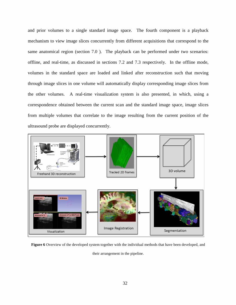
and prior volumes to a single standard image space. The fourth component is a playback
mechanism to view image slices concurrently from different acquisitions that correspond to the
same anatomical region (section 7.0 ). The playback can be performed under two scenarios:
offline, and real-time, as discussed in sections 7.2 and 7.3 respectively. In the offline mode,
volumes in the standard space are loaded and linked after reconstruction such that moving
through image slices in one volume will automatically display corresponding image slices from
the other volumes. A real-time visualization system is also presented, in which, using a
correspondence obtained between the current scan and the standard image space, image slices
from multiple volumes that correlate to the image resulting from the current position of the
ultrasound probe are displayed concurrently.
Figure 6 Overview of the developed system together with the individual methods that have been developed, and
their arrangement in the pipeline.
32

The combination of the four components described above will provide the ability to
accurately monitor changes in anatomical structures, thus enabling preventive and therapeutic
strategies for nerve regeneration and chronic rejection (CR) in Composite Tissue
Allotransplantation (CTA). The registration algorithm is also applied in this dissertation to MR
images in diseases of the elderly such as vascular dementia, Alzheimer’s, and late life
depression.
3.3 AUTOMATED IMAGE ANALYSIS
A critical first step before attempting to identify the growing axon cone of the regenerating nerve
is identification of individual fascicles in HRUS images of a normal nerve such as the median
nerve and developing automated methods to reliably discriminate fascicles from other similar
structures (such as tendons). Likewise, it is of utmost importance for both basic neuroscience
and clinical research that reliable and efficient methods for accurately segmenting the
hippocampus in MR images of the brain are developed, to aid in studying the function and
structure of the hippocampus in the living human brain and its effects on various brain related
conditions.
Interpreting medical images generally requires expert manual interpretation to separate
the target anatomy and relevant contextual information from the noise. This process, which
generally involves examining one slice at a time, is tedious and time consuming, especially with
large 3D datasets such as those produced by MRI and volumetric ultrasound. Hence,
computerized image analysis to extract information with little or no manual intervention is of
critical importance. Most conventional automated methods, such as the ones mentioned in
33
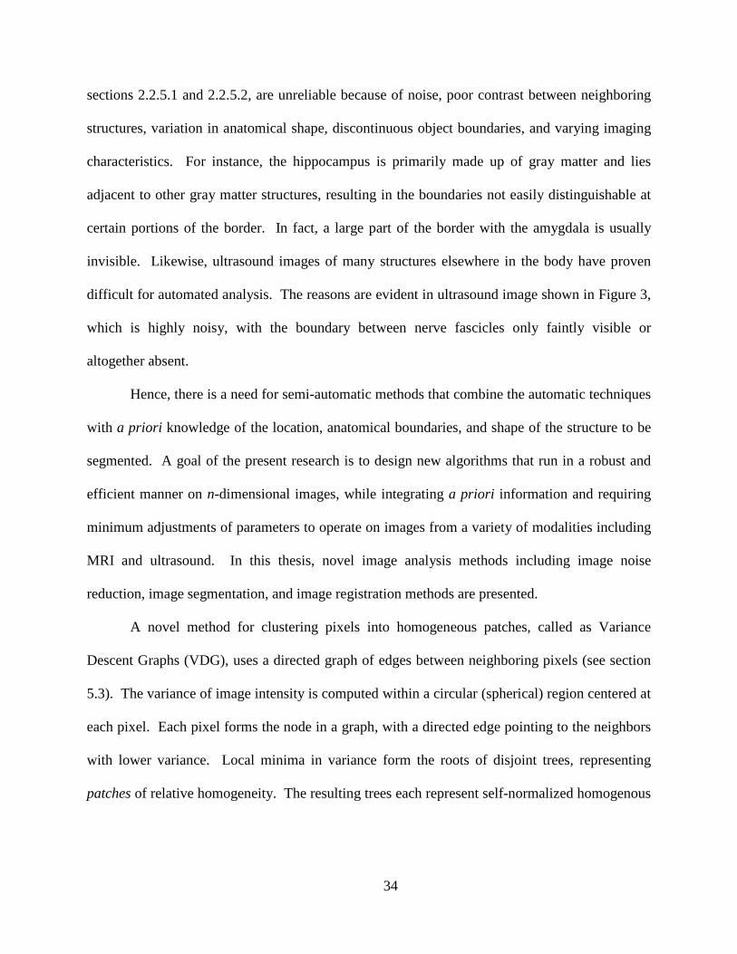
sections 2.2.5.1 and 2.2.5.2, are unreliable because of noise, poor contrast between neighboring
structures, variation in anatomical shape, discontinuous object boundaries, and varying imaging
characteristics. For instance, the hippocampus is primarily made up of gray matter and lies
adjacent to other gray matter structures, resulting in the boundaries not easily distinguishable at
certain portions of the border. In fact, a large part of the border with the amygdala is usually
invisible. Likewise, ultrasound images of many structures elsewhere in the body have proven
difficult for automated analysis. The reasons are evident in ultrasound image shown in Figure 3,
which is highly noisy, with the boundary between nerve fascicles only faintly visible or
altogether absent.
Hence, there is a need for semi-automatic methods that combine the automatic techniques
with a priori knowledge of the location, anatomical boundaries, and shape of the structure to be
segmented. A goal of the present research is to design new algorithms that run in a robust and
efficient manner on n-dimensional images, while integrating a priori information and requiring
minimum adjustments of parameters to operate on images from a variety of modalities including
MRI and ultrasound. In this thesis, novel image analysis methods including image noise
reduction, image segmentation, and image registration methods are presented.
A novel method for clustering pixels into homogeneous patches, called as Variance
Descent Graphs (VDG), uses a directed graph of edges between neighboring pixels (see section
5.3). The variance of image intensity is computed within a circular (spherical) region centered at
each pixel. Each pixel forms the node in a graph, with a directed edge pointing to the neighbors
with lower variance. Local minima in variance form the roots of disjoint trees, representing
patches of relative homogeneity. The resulting trees each represent self-normalized homogenous
34
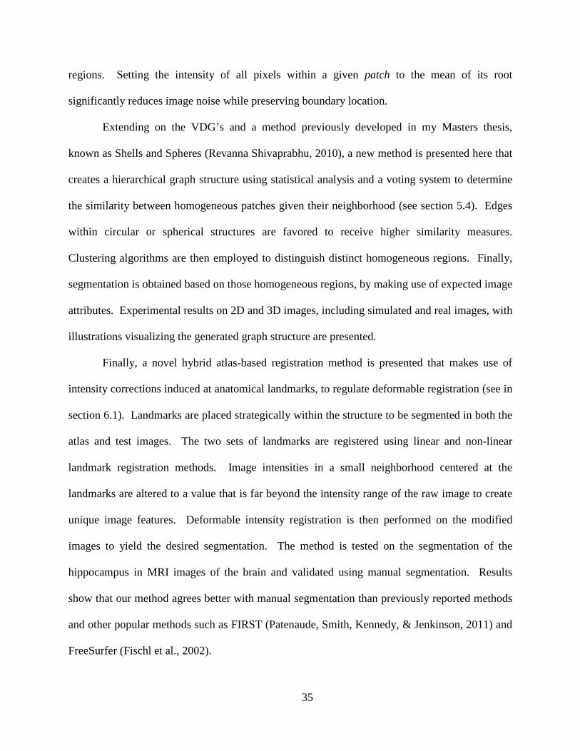
regions. Setting the intensity of all pixels within a given patch to the mean of its root
significantly reduces image noise while preserving boundary location.
Extending on the VDG’s and a method previously developed in my Masters thesis,
known as Shells and Spheres (Revanna Shivaprabhu, 2010), a new method is presented here that
creates a hierarchical graph structure using statistical analysis and a voting system to determine
the similarity between homogeneous patches given their neighborhood (see section 5.4). Edges
within circular or spherical structures are favored to receive higher similarity measures.
Clustering algorithms are then employed to distinguish distinct homogeneous regions. Finally,
segmentation is obtained based on those homogeneous regions, by making use of expected image
attributes. Experimental results on 2D and 3D images, including simulated and real images, with
illustrations visualizing the generated graph structure are presented.
Finally, a novel hybrid atlas-based registration method is presented that makes use of
intensity corrections induced at anatomical landmarks, to regulate deformable registration (see in
section 6.1). Landmarks are placed strategically within the structure to be segmented in both the
atlas and test images. The two sets of landmarks are registered using linear and non-linear
landmark registration methods. Image intensities in a small neighborhood centered at the
landmarks are altered to a value that is far beyond the intensity range of the raw image to create
unique image features. Deformable intensity registration is then performed on the modified
images to yield the desired segmentation. The method is tested on the segmentation of the
hippocampus in MRI images of the brain and validated using manual segmentation. Results
show that our method agrees better with manual segmentation than previously reported methods
and other popular methods such as FIRST (Patenaude, Smith, Kennedy, & Jenkinson, 2011) and
FreeSurfer (Fischl et al., 2002).
35

4.0 FREEHAND 3D RECONSTRUCTION
The various techniques available to generate volumetric ultrasound were discussed in section
2.2.3. In this dissertation, freehand 3D reconstruction is employed to generate volumetric
ultrasound images. Figure 7 shows the overview of the freehand ultrasound 3D volume
reconstruction system. As the ultrasound probe is maneuvered over the target anatomical
structure, position and orientation of the probe are recorded using a Micron Tracker, a
commercially available tracking system from Claron Technology Inc.("Micron Tracker,"). For
each B-scan, individual, 2D image is acquired digitally from the ultrasound scanner using a
video frame grabber. The 2D images are stamped with meta-data indicating the time of
acquisition, as well as the position and orientation of the scan obtained from the tracking system.
A 3D volume is reconstructed by placing the 2D images within a 3D space based on the
information in this meta-data.
When the 2D images are consolidated into a 3D space, a particular voxel in the 3D
volume may either be intersected by pixels from more than one 2D image or may not be
intersected by any pixel. As suggested in (Rohling et al., 1999), the former problem, known as
‘bin-filling’, can be solved by combining data in the overlapping pixels (compounding). The
latter problem, known as ‘hole-filling’, can be solved by inferring values for the missing data
using information of the voxel’s neighbors (interpolation). Bin-filling and hole-filling techniques
36
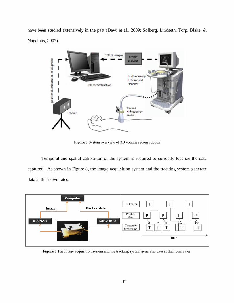
have been studied extensively in the past (Dewi et al., 2009; Solberg, Lindseth, Torp, Blake, &
Nagelhus, 2007).
Figure 7 System overview of 3D volume reconstruction
Temporal and spatial calibration of the system is required to correctly localize the data
captured. As shown in Figure 8, the image acquisition system and the tracking system generate
data at their own rates.
Figure 8 The image acquisition system and the tracking system generates data at their own rates.
37
The aim of temporal calibration is to estimate the latency between the two systems and provide a
single time coordinate. The ultrasound probe is moved vertically in a tank of water in a smooth
periodic motion, such that the bottom of the tank appears in the image as a horizontal line that
moves up and down. The tracker and video streams are recorded simultaneously. The horizontal
line is segmented using automated image analysis and the temporal relation found where there is
maximum correlation between the movement of the line segment and the tracker data (F.
Rousseau, Hellier, & Barillot, 2006). Figure 9 shows the data recorded from the tracking and
imaging systems. The blue plot in both the graphs denotes data from the tracking data. The red
plot in the top graph denotes line segmented in the image before calibration. Maximum
correlation of the two plots was detected at an offset of 0.244 seconds. The green plot in the
bottom graph denotes the image data after it is compensated for the time offset.
38
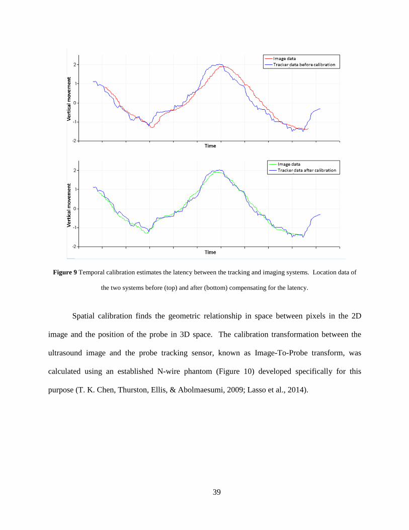
Figure 9 Temporal calibration estimates the latency between the tracking and imaging systems. Location data of
the two systems before (top) and after (bottom) compensating for the latency.
Spatial calibration finds the geometric relationship in space between pixels in the 2D
image and the position of the probe in 3D space. The calibration transformation between the
ultrasound image and the probe tracking sensor, known as Image-To-Probe transform, was
calculated using an established N-wire phantom (Figure 10) developed specifically for this
purpose (T. K. Chen, Thurston, Ellis, & Abolmaesumi, 2009; Lasso et al., 2014).
39
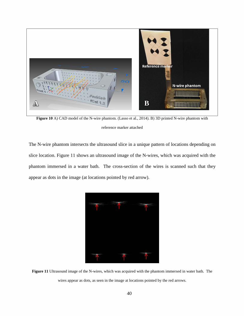
Figure 10 A) CAD model of the N-wire phantom. (Lasso et al., 2014). B) 3D printed N-wire phantom with
reference marker attached
The N-wire phantom intersects the ultrasound slice in a unique pattern of locations depending on
slice location. Figure 11 shows an ultrasound image of the N-wires, which was acquired with the
phantom immersed in a water bath. The cross-section of the wires is scanned such that they
appear as dots in the image (at locations pointed by red arrow).
Figure 11 Ultrasound image of the N-wires, which was acquired with the phantom immersed in water bath. The
wires appear as dots, as seen in the image at locations pointed by the red arrows.
A B
40
By detecting the intersecting points in the ultrasound image as the probe is maneuvered over the
phantom, it is possible to calculate the calibration transformation. The reader is referred to (T. K.
Chen et al., 2009) for the theory concerning the estimation of calibration parameters. Automatic
segmentation and pattern recognition algorithms also described in (T. K. Chen et al., 2009) were
used to detect the cross-section of the wires in the ultrasound image.
The implementation was performed using PLUS (Public software Library for UltraSound
imaging research) (Lasso et al., 2014), an open source toolkit containing library functions and
applications for tracked ultrasound image acquisition, calibration, and processing. PLUS
conveniently combines calibration methods (temporal and spatial), recording tracked ultrasound
images and volume reconstruction algorithms. The ultrasound images were saved as an extension
to the meta-IO standard image file format (*.mha, *.mhd), with the image header containing
tracking information, including image orientation, transforms from the tracker, and timestamps,
as described above. PLUS currently supports a variety of image acquisition devices such as
Ultrasonix, BK ultrasound systems, and various frame grabbers. It also supports a wide range of
tracking systems such as Ascension, NDI, Claron, Phidget, CHRobotics pose tracking devices,
and any device with OpenIGTLink output. The advantage of using such a library is that the
system developed does not depend on any single device configuration. Using PLUS, it is very
easy to switch to a different combination of image acquisition and tracking devices.
41

Figure 12 3D rendering of the segmentation of the wires from the freehand reconstructed volume of the N-wire
phantom. Also shown are three orthogonal slices.
The freehand 3D reconstruction system was tested on the N-wire phantom made up of
three layers of three wires each (with each set of three wires forming the shape of an “N”, hence
the term “N-wire). Figure 12 shows 3D rendering of the segmentation of the wires from the
reconstructed volume. Segmentation was performed using the intensity threshold method
mentioned above. Also shown are three orthogonal slices through the ultrasound data to provide
a spatial context. We can clearly see the N-shape of the wires in the reconstructed image. The
width of the middle N-wire (distance between the parallel lines), and the height between the first
and third N-wire were measured in the reconstructed image. The measured width and height
were 19.6 mm and 20.2 mm respectively, while the true physical distances were both 20 mm.
42

Figure 13D shows an image slice retrieved from a reconstructed 3D US volume of the
phantom corresponding to the live US image seen in Figure 13C (J. Wang et al., 2014). The
quality of the reconstructed slice suffers from the problems outlined above.
Figure 13 (A) US probe tracked by markers mounted on it. (B) 3D model of individual 2D US images stacked in a
3D space based on the recorded location and orientation of the US probe. (C) Live US image. (D) US image slice
retrieved from a previously reconstructed US volume corresponding to the live US image.
A B
C D
43
5.0 IMAGE SEGMENTATION
In this section, we present novel image segmentation methods including a medial based
segmentation method, a method that clusters pixels into homogenous patches, and a graph based
segmentation method.
In sections 5.1 and 5.2, we present a medial based segmentation method, which extends a
method previously developed (Revanna Shivaprabhu, 2010) to extract medial points based on the
divergence of the direction function to the nearest boundary as it changes across medial ridges.
The direction function is determined by analyzing the mean and variance of intensity within
asymmetric pairs of adjacent spherical regions. The medial points detected are clustered to
extract features including scale, orientation and medial dimensionality. These are then organized
as a graph structure and partitioned in the feature space using spectral analysis. A learning based
approach to find similar partitions in a test image is presented.
In section 5.3, we present a novel and relatively simple method for clustering pixels into
homogeneous patches using a directed graph of edges between neighboring pixels. The method
works in n-dimensions and requires only a single parameter, the radius of the circular regions
used to compute variance.
In section 5.4, we present an n-dimensional automated method, which creates a
hierarchical graph structure that makes use of statistical analysis and a voting system to
determine the similarity between previously generated homogeneous patches given their
44
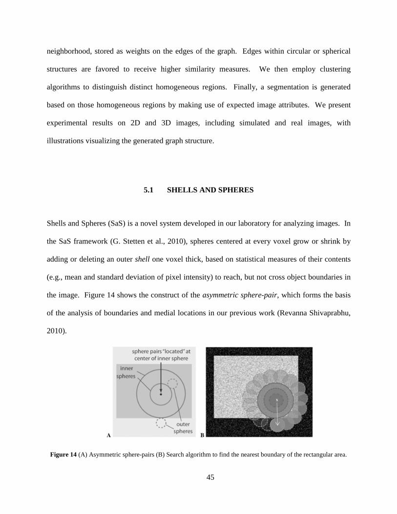
neighborhood, stored as weights on the edges of the graph. Edges within circular or spherical
structures are favored to receive higher similarity measures. We then employ clustering
algorithms to distinguish distinct homogeneous regions. Finally, a segmentation is generated
based on those homogeneous regions by making use of expected image attributes. We present
experimental results on 2D and 3D images, including simulated and real images, with
illustrations visualizing the generated graph structure.
5.1 SHELLS AND SPHERES
Shells and Spheres (SaS) is a novel system developed in our laboratory for analyzing images. In
the SaS framework (G. Stetten et al., 2010), spheres centered at every voxel grow or shrink by
adding or deleting an outer shell one voxel thick, based on statistical measures of their contents
(e.g., mean and standard deviation of pixel intensity) to reach, but not cross object boundaries in
the image. Figure 14 shows the construct of the asymmetric sphere-pair, which forms the basis
of the analysis of boundaries and medial locations in our previous work (Revanna Shivaprabhu,
2010).
Figure 14 (A) Asymmetric sphere-pairs (B) Search algorithm to find the nearest boundary of the rectangular area.
45

An asymmetric sphere-pair consists of an “outer” sphere (dashed circle) held at a
constant, small radius, adjacent to an “inner” sphere (solid circle) that increases in radius. The
location of the asymmetric sphere-pair is considered to be the center of its inner-sphere, and thus
a family of possible sizes for the inner-sphere and orientations for the outer-sphere for a given
inner-sphere size are possible at each location. Two such pairs at a given location within a
rectangular object are shown in Figure 14A, with the larger inner-sphere correctly finding the
boundary of the object in conjunction with one of its outer-spheres. The constant radius of the
outer sphere is chosen to be small enough to provide sufficient boundary curvature while still
being large enough to represent a statistically significant population. As the inner-sphere is
grown to each new radius, every possible orientation of outer-sphere is tested, and an overall
measure of boundary strength is used to identify the boundary. The optimum sphere- pair should
have its inner-sphere just touching the nearest boundary and its outer- sphere just on the other
side of that boundary.
To permit the SaS framework to find boundaries, a measurement of boundary strength
based on the samples of voxel intensity in adjoining spherical regions is required. The measure
of boundary strength we choose is the 𝑑𝑑′ (d-prime) statistic, commonly used in signal detection
to express the difference between the mean of a signal and the distribution of noise, in units of
standard deviation. It is applied to the intensity of voxels within the inner-sphere and outer-
sphere of a given sphere-pair. Since the standard deviations of the inner-sphere and outer-sphere
samples are not expected to be necessarily equal, the concept of pooled standard deviation is
borrowed from the Student’s t-test to yield the following definition of 𝑑𝑑′:
𝑑𝑑′ = 𝑋𝑋𝑖𝑖 − 𝑋𝑋𝑜𝑜
(𝑆𝑆𝑖𝑖2 + 𝑆𝑆𝑜𝑜2)/2 2
46

where 𝑋𝑋 and S are the means and standard deviations of voxel intensity for the voxel samples in
the inner-sphere (i) and outer-sphere (o).
Using the 𝑑𝑑′ statistic as a measure of boundary strength, a search is performed for the
boundary nearest to a particular location x using the algorithm depicted in Figure 14B. Starting
with an inner-sphere of the same radius as the outer-sphere, the inner sphere is expanded,
checking each possible orientation of adjacent outer-sphere. A discrete set of the centers of such
outer-spheres is obtained from the shell centered at x whose radius is the sum of the outer-sphere
and inner- sphere radii. At each inner-sphere radius (scale) the sphere-pair with the maximum 𝑑𝑑′
statistic is chosen to represent the distance r(x) and radial direction 𝒓𝒓(x) to the putative nearest
boundary (the ‘^’ denotes a unit vector).
The direction vector changes abruptly when one crosses the medial manifold, as one
boundary suddenly becomes closer than the other. This amounts to a singularity in the
divergence of the direction vector in the continuous domain (Siddiqi & Pizer, 2008). Since
medical images are generally discrete and the asymmetric sphere-pair represents a forced choice
at every voxel location and scale to a single nearest boundary, neighboring voxels whose
direction vectors 𝒓𝒓(x) change significantly infer that the actual medial location is somewhere
between the two voxels. This strategy is implemented by checking the winning sphere-pairs at
each inner- sphere radius (scale) against their immediate neighbors. Since, for a medial location,
the distance to the opposing boundaries is equal, the scale of the two neighboring sphere-pairs
should be equal, and thus all the sphere-pairs can be searched one scale at one time. When
neighboring voxel locations whose sphere-pairs have a sufficiently high 𝑑𝑑′ and whose direction
vectors yield a dot product that is sufficiently negative are found (to ensure that the two
boundaries are not actually neighboring segments of the same boundary region), it implies that a
47
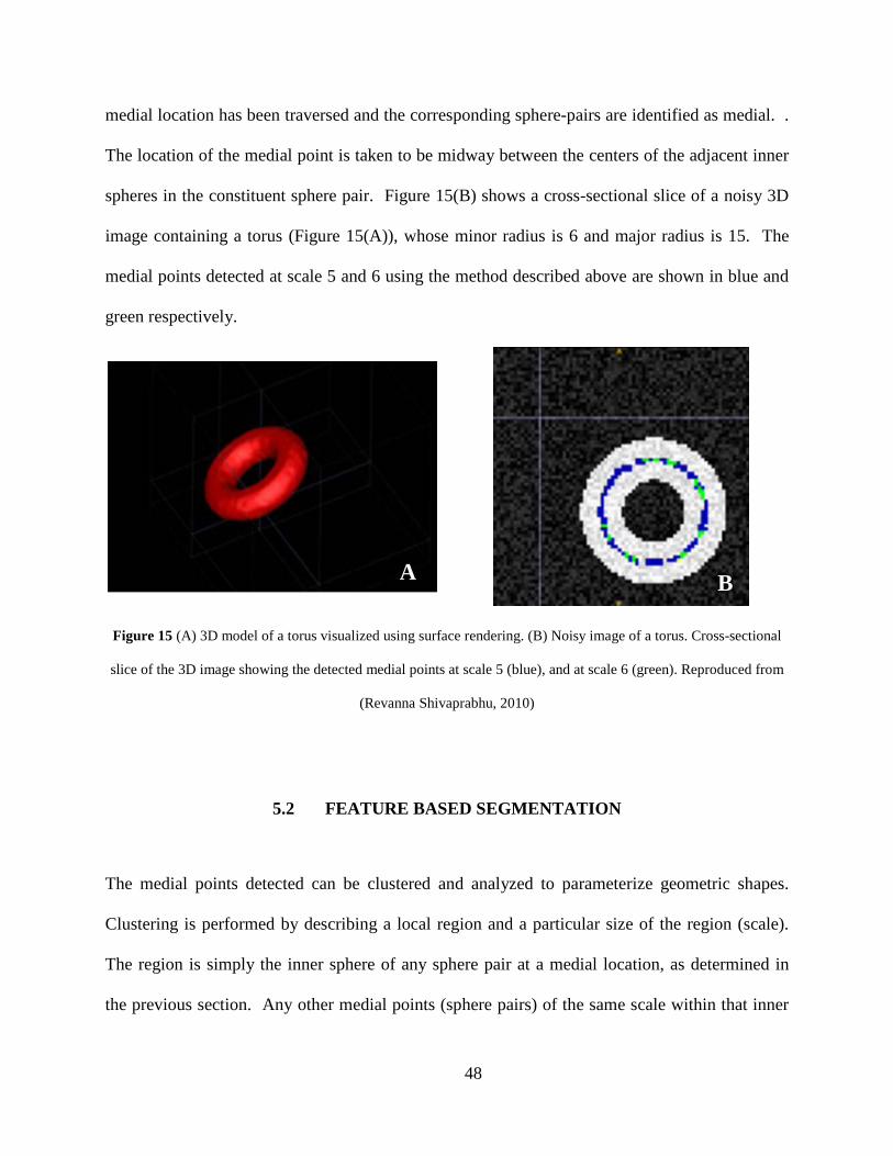
medial location has been traversed and the corresponding sphere-pairs are identified as medial. .
The location of the medial point is taken to be midway between the centers of the adjacent inner
spheres in the constituent sphere pair. Figure 15(B) shows a cross-sectional slice of a noisy 3D
image containing a torus (Figure 15(A)), whose minor radius is 6 and major radius is 15. The
medial points detected at scale 5 and 6 using the method described above are shown in blue and
green respectively.
Figure 15 (A) 3D model of a torus visualized using surface rendering. (B) Noisy image of a torus. Cross-sectional
slice of the 3D image showing the detected medial points at scale 5 (blue), and at scale 6 (green). Reproduced from
(Revanna Shivaprabhu, 2010)
5.2 FEATURE BASED SEGMENTATION
The medial points detected can be clustered and analyzed to parameterize geometric shapes.
Clustering is performed by describing a local region and a particular size of the region (scale).
The region is simply the inner sphere of any sphere pair at a medial location, as determined in
the previous section. Any other medial points (sphere pairs) of the same scale within that inner
A B
48

sphere are considered to be in the cluster. Thus, a cluster 𝐶𝐶𝑟𝑟(𝒙𝒙) at pixel location 𝒙𝒙 is defined as
𝐶𝐶𝑟𝑟(𝒙𝒙) = [ 𝑆𝑆𝑟𝑟(𝒙𝒙) ∩ M ], where 𝑆𝑆𝑟𝑟(𝒙𝒙) is an inner sphere of radius 𝑐𝑐 centered at image pixel 𝒙𝒙, and
M is the set of all medial points. Associated with each medial point is a direction vector pointing
to the nearest boundary. A given population of direction vectors may be examined to obtain a
compact and versatile representation of the local shape, following methods developed by Stetten
and Pizer (G. D. Stetten & Pizer, 1999). Eigenanalysis on the cluster of direction vectors,
computed using the covariance matrix D given by:
𝐷𝐷 = 1𝑖𝑖𝑑𝑖𝑖𝑑𝑖𝑖𝑇𝑇𝑛𝑛
𝑖𝑖=1
3
where 𝑑𝑖𝑖 is a population of 𝑖𝑖 unit directional vectors, results in as many eigenvalues and
eigenvectors as the dimension of the image. Assuming we are working in N dimensions, the
eigenvalues may be denoted as 𝜆𝜆1, 𝜆𝜆2……… 𝜆𝜆𝑁𝑁 and their corresponding eigenvectors may be
denoted as 𝑎𝑎1,𝑎𝑎2 … .𝑎𝑎𝑁𝑁. Since D is a positive definite symmetric matrix, its eigenvalues are all
positive and sum to 1, i.e. 𝜆𝜆1 + 𝜆𝜆2 + ⋯+ 𝜆𝜆𝑁𝑁 = 1. If we arrange the eigenvalues such that 𝜆𝜆1 ≤
𝜆𝜆2 ≤ ⋯ ≤ 𝜆𝜆𝑁𝑁 , then their relative values can be used to represent dimensionality of the medial
manifold, and their corresponding eigenvectors 𝑎𝑎1,𝑎𝑎2 … .𝑎𝑎𝑁𝑁 can represent the manifold’s
orientation. In the case of 3D, 𝑎𝑎1and 𝑎𝑎2 can be used to describe the dimensionality of an object.
Note that it is sufficient to compute 𝜆𝜆1 and 𝜆𝜆2 since 𝜆𝜆3 = 1 − (𝜆𝜆1 + 𝜆𝜆2).
A feature vector V comprised of the location of the medial point x, the radius of the inner
sphere s centered at the medial point, and the eigenvalues 𝜆𝜆𝑖𝑖, 𝑖𝑖 = 1 … .𝑁𝑁 − 1 computed at the
medial point, characterizes the shape of the object locally in the vicinity of the medial point. A
feature vector V may be formed at each medial point and the combination of all vectors
represents the complete object. Thus, the shape of the object, originally represented as group of
49

voxels in the Cartesian image space I, is transformed to data points in feature space F
represented by feature vectors V
I : [𝑥𝑥, 𝑦𝑦, 𝑧𝑧] → F : V = 𝒙𝒙𝑖𝑖𝜆𝜆𝑖𝑖 4
The feature space may be modeled as a complete (simple undirected) graph G = (𝓝𝓝, E),
with the feature vectors V forming the nodes/vertices (𝓝𝓝) of the graph. Every node in the graph
(𝒩𝒩𝑖𝑖) is connected to every other node by weighted edges (E). The weight on each edge, denoted
as w(𝒩𝒩𝑖𝑖, 𝒩𝒩𝑗𝑗), is a function of similarity between the two nodes, with the weight being larger if
the nodes are dissimilar. A number of similarity measures can be used. For example, in (Egghe,
2009) similarity measures such as Jaccard, cosine, Dice, and several related overlap measures
have been derived for vectors from set-theoretic similarity measures.
The graph G may be partitioned into groups using normalized cuts criterion (Shi &
Malik, 2000), which measures both the total dissimilarity between groups as well as the total
similarity within groups. A partition is obtained when the edges connecting the two dissimilar
groups are removed. The degree of dissimilarity between the two groups (A and B), called the
cut, can be computed as the total weight of the edges that have been removed, i.e.,
𝑐𝑐𝑐𝑐𝑡𝑡(𝐴𝐴,𝐵𝐵) = 𝑤𝑤(𝒩𝒩𝑖𝑖 ,𝒩𝒩𝑗𝑗)𝒩𝒩𝑖𝑖∈𝐴𝐴,𝒩𝒩𝑗𝑗∈𝐵𝐵
5
In (Shi & Malik, 2000), Shi and Malik have proposed a normalized cut criterion - an
unbiased measure of disassociation between subgroups of a graph – having the property that
minimizing normalized cut leads directly to maximizing the normalized association, which is an
unbiased measure for total association within subgroups. A generalized eigenvalue system for
50

computing the minimum normalized cut has also been proposed. The normalized cut (Ncut) and
normalized association (Nassoc) are given by:
𝑁𝑁𝑐𝑐𝑐𝑐𝑡𝑡(𝐴𝐴,𝐵𝐵) = 𝑐𝑐𝑐𝑐𝑡𝑡(𝐴𝐴,𝐵𝐵)
𝑎𝑎𝑖𝑖𝑖𝑖𝑐𝑐𝑐𝑐(𝐴𝐴,𝓝𝓝)+
𝑐𝑐𝑐𝑐𝑡𝑡(𝐴𝐴,𝐵𝐵)𝑎𝑎𝑖𝑖𝑖𝑖𝑐𝑐𝑐𝑐(𝐵𝐵,𝓝𝓝)
6
𝑁𝑁𝑎𝑎𝑖𝑖𝑖𝑖𝑐𝑐𝑐𝑐(𝐴𝐴,𝐵𝐵) = 𝑎𝑎𝑖𝑖𝑖𝑖𝑐𝑐𝑐𝑐(𝐴𝐴,𝐴𝐴)𝑎𝑎𝑖𝑖𝑖𝑖𝑐𝑐𝑐𝑐(𝐴𝐴,𝓝𝓝)
+ 𝑎𝑎𝑖𝑖𝑖𝑖𝑐𝑐𝑐𝑐(𝐵𝐵,𝐵𝐵)𝑎𝑎𝑖𝑖𝑖𝑖𝑐𝑐𝑐𝑐(𝐵𝐵,𝓝𝓝)
7
where,
𝑎𝑎𝑖𝑖𝑖𝑖𝑐𝑐𝑐𝑐(𝐴𝐴,𝓝𝓝) = 𝑤𝑤(𝒩𝒩𝑖𝑖,𝒩𝒩𝑗𝑗)𝒩𝒩𝑖𝑖∈𝐴𝐴,𝒩𝒩𝑗𝑗∈𝓝𝓝
8
is the total connection from nodes in A to all the nodes in the graph.
By partitioning the graph according to the criteria described above, the global shape of
the object will be divided into distinct partitions in feature space. Figure 16(B) shows the result
of applying the method described above to a binary segmentation of the hippocampus (Figure
16(A)). The medial manifold is represented by cubes in the figure. The Eigenvectors are
represented by arrows and the partitions obtained after applying the normalized cut method are
shown in different colors. The following similarity measure was used to generate the weight on
each edge:
𝑤𝑤𝒩𝒩𝑖𝑖 ,𝒩𝒩𝑗𝑗 = −log 1 −1𝑖𝑖
|𝑣𝑣𝑖𝑖𝑘𝑘 − 𝑣𝑣𝑗𝑗𝑘𝑘|𝑣𝑣𝑖𝑖𝑖𝑖𝑚𝑚𝑘𝑘 − 𝑣𝑣𝑖𝑖𝑖𝑖𝑛𝑛𝑘𝑘
𝑛𝑛
𝑘𝑘=1
9
where 𝑣𝑣𝑘𝑘 is the 𝑘𝑘th feature in the feature vector V that is stored at each node 𝒩𝒩, 𝑣𝑣𝑖𝑖𝑖𝑖𝑚𝑚 and 𝑣𝑣𝑖𝑖𝑖𝑖𝑛𝑛
are the maximum and minimum values of the 𝑘𝑘th feature, which are obtained from all available
data points. Equation 9 takes into consideration the dynamic range of each feature, by
normalizing each feature individually. We include a logarithm to compress the total dynamic
51
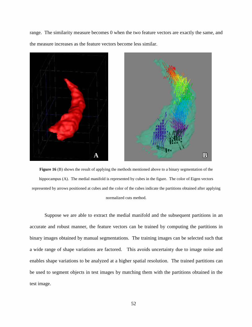
range. The similarity measure becomes 0 when the two feature vectors are exactly the same, and
the measure increases as the feature vectors become less similar.
Figure 16 (B) shows the result of applying the methods mentioned above to a binary segmentation of the
hippocampus (A). The medial manifold is represented by cubes in the figure. The color of Eigen vectors
represented by arrows positioned at cubes and the color of the cubes indicate the partitions obtained after applying
normalized cuts method.
Suppose we are able to extract the medial manifold and the subsequent partitions in an
accurate and robust manner, the feature vectors can be trained by computing the partitions in
binary images obtained by manual segmentations. The training images can be selected such that
a wide range of shape variations are factored. This avoids uncertainty due to image noise and
enables shape variations to be analyzed at a higher spatial resolution. The trained partitions can
be used to segment objects in test images by matching them with the partitions obtained in the
test image.
A B
52

However, the method described above is prone to error, mostly because feature vectors
and partitions similar to those in the training dataset need to be identified in the raw test image as
well. Although medial manifolds can be computed reliably using SaS in binary images, using
asymmetric sphere pairs of SaS to identify boundaries in gray scale images can be challenging,
especially when the neighboring region is smaller than the size of the outer sphere. For example,
at the location pointed by the red arrow in Figure 17, the boundary separating the hippocampus
and the adjacent amygdala is very thin. The outer sphere in such cases can encompass both the
thin tissue that separates the two structures and the neighboring amygdala, thereby failing to
identify the boundary. In addition, modest deviation in the expected shape of the target structure
can alter the medial manifold considerably, leading to the generation of irregular partitions
previously unseen during training. Missing boundaries such as those that appear in the
ultrasound images of the median nerve (Figure 17B) also results in unpredictable medial
manifolds. Also, Eigen analysis of direction vectors does not account for the occurrence of
endness. Endness is the extremity of medial manifolds, where the inner sphere osculates with
the boundary, i.e., where the curvature of the inner sphere matches the curvature of the boundary
53
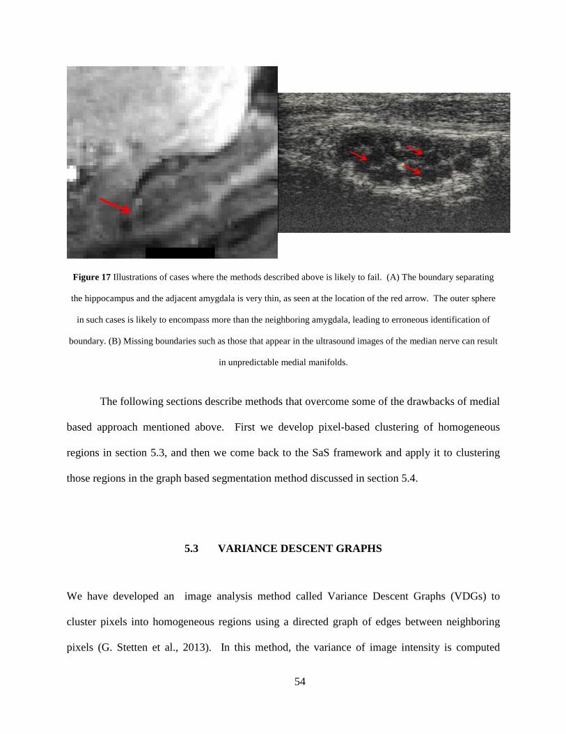
Figure 17 Illustrations of cases where the methods described above is likely to fail. (A) The boundary separating
the hippocampus and the adjacent amygdala is very thin, as seen at the location of the red arrow. The outer sphere
in such cases is likely to encompass more than the neighboring amygdala, leading to erroneous identification of
boundary. (B) Missing boundaries such as those that appear in the ultrasound images of the median nerve can result
in unpredictable medial manifolds.
The following sections describe methods that overcome some of the drawbacks of medial
based approach mentioned above. First we develop pixel-based clustering of homogeneous
regions in section 5.3, and then we come back to the SaS framework and apply it to clustering
those regions in the graph based segmentation method discussed in section 5.4.
5.3 VARIANCE DESCENT GRAPHS
We have developed an image analysis method called Variance Descent Graphs (VDGs) to
cluster pixels into homogeneous regions using a directed graph of edges between neighboring
pixels (G. Stetten et al., 2013). In this method, the variance of image intensity is computed
54
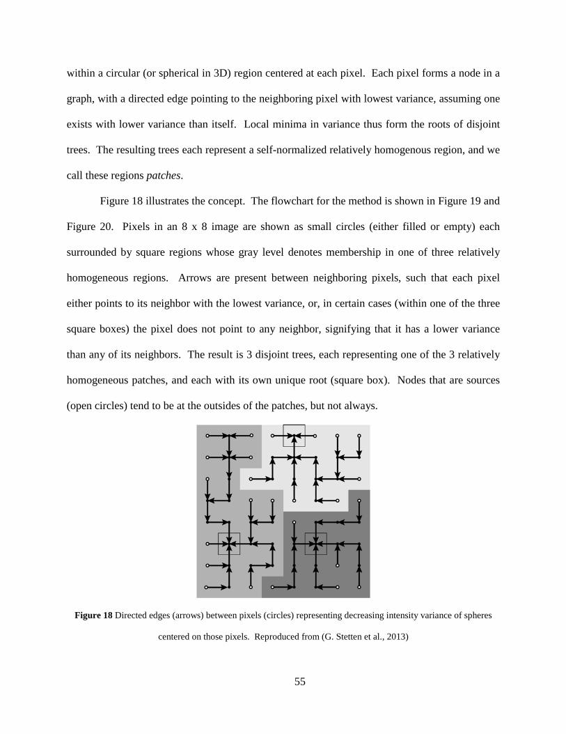
within a circular (or spherical in 3D) region centered at each pixel. Each pixel forms a node in a
graph, with a directed edge pointing to the neighboring pixel with lowest variance, assuming one
exists with lower variance than itself. Local minima in variance thus form the roots of disjoint
trees. The resulting trees each represent a self-normalized relatively homogenous region, and we
call these regions patches.
Figure 18 illustrates the concept. The flowchart for the method is shown in Figure 19 and
Figure 20. Pixels in an 8 x 8 image are shown as small circles (either filled or empty) each
surrounded by square regions whose gray level denotes membership in one of three relatively
homogeneous regions. Arrows are present between neighboring pixels, such that each pixel
either points to its neighbor with the lowest variance, or, in certain cases (within one of the three
square boxes) the pixel does not point to any neighbor, signifying that it has a lower variance
than any of its neighbors. The result is 3 disjoint trees, each representing one of the 3 relatively
homogeneous patches, and each with its own unique root (square box). Nodes that are sources
(open circles) tend to be at the outsides of the patches, but not always.
Figure 18 Directed edges (arrows) between pixels (circles) representing decreasing intensity variance of spheres
centered on those pixels. Reproduced from (G. Stetten et al., 2013)
55
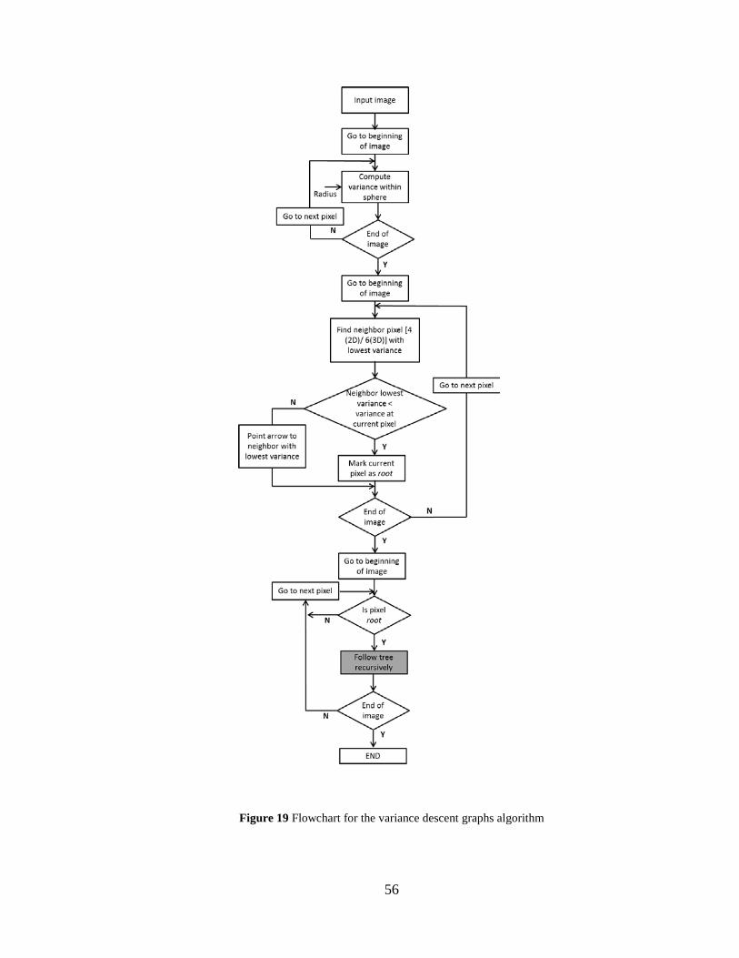
Figure 19 Flowchart for the variance descent graphs algorithm
56

Figure 20 Flowchart for the recursive function ‘Follow tree recursively’ used in the flowchart shown in
Figure 19
The method works in n-dimensions, is self-normalizing, and requires only a single
parameter: the radius of the circular regions used to compute variance for each pixel. Replacing
the pixel intensity in each VDG patch with the mean intensity of the sphere belonging to the
corresponding root represents a compression of useful information in the image, reducing
intensity noise while preserving useful intensity and boundary information.
57

Methods that reduce noise and perform data dimensionality reduction are extremely
useful when analyzing ultrasound images. Due to the nature of ultrasound image acquisition, the
signal-to-noise ratio (SNR) in ultrasound images is amongst the lowest in medical imaging. High
noise and variability in image intensity in these images make reliable automated image analysis
tasks particularly difficult. High data dimensionality also poses challenges to automated image
analysis. Commonly, image segmentation algorithms work at the pixel level, i.e., every pixel of
the image is analyzed by the algorithm. For n pixels, computation time and memory usage, are
often proportional to somewhere from n and n2, depending on the algorithm, making such
algorithms impractical where a large number of 2D images are obtained over the course of a
single scan, or when 3D ultrasound datasets are to be analyzed. Thus reducing noise and the
number of elements to analyze by first forming patches is beneficial in a number of ways.
58
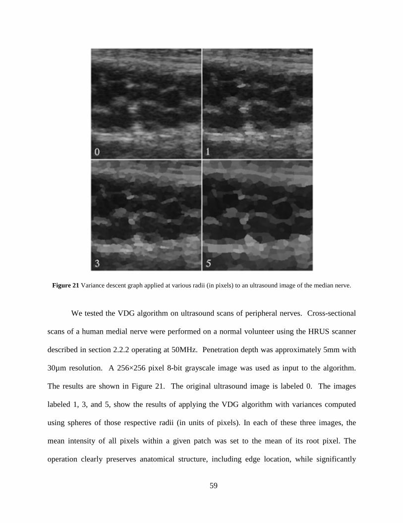
Figure 21 Variance descent graph applied at various radii (in pixels) to an ultrasound image of the median nerve.
We tested the VDG algorithm on ultrasound scans of peripheral nerves. Cross-sectional
scans of a human medial nerve were performed on a normal volunteer using the HRUS scanner
described in section 2.2.2 operating at 50MHz. Penetration depth was approximately 5mm with
30µm resolution. A 256×256 pixel 8-bit grayscale image was used as input to the algorithm.
The results are shown in Figure 21. The original ultrasound image is labeled 0. The images
labeled 1, 3, and 5, show the results of applying the VDG algorithm with variances computed
using spheres of those respective radii (in units of pixels). In each of these three images, the
mean intensity of all pixels within a given patch was set to the mean of its root pixel. The
operation clearly preserves anatomical structure, including edge location, while significantly
59
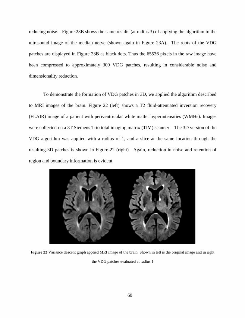
reducing noise. Figure 23B shows the same results (at radius 3) of applying the algorithm to the
ultrasound image of the median nerve (shown again in Figure 23A). The roots of the VDG
patches are displayed in Figure 23B as black dots. Thus the 65536 pixels in the raw image have
been compressed to approximately 300 VDG patches, resulting in considerable noise and
dimensionality reduction.
To demonstrate the formation of VDG patches in 3D, we applied the algorithm described
to MRI images of the brain. Figure 22 (left) shows a T2 fluid-attenuated inversion recovery
(FLAIR) image of a patient with periventricular white matter hyperintensities (WMHs). Images
were collected on a 3T Siemens Trio total imaging matrix (TIM) scanner. The 3D version of the
VDG algorithm was applied with a radius of 1, and a slice at the same location through the
resulting 3D patches is shown in Figure 22 (right). Again, reduction in noise and retention of
region and boundary information is evident.
Figure 22 Variance descent graph applied MRI image of the brain. Shown in left is the original image and in right
the VDG patches evaluated at radius 1
60
The next section describes a graph based method that further clusters the VDG patches in
a hierarchical approach resulting in the identification of larger target structures.
5.4 GRAPH BASED TECHNIQUES
The VDG patches computed in the previous section (5.3) reduces noise in the image while
preserving useful intensity and boundary information. There are far fewer patches than original
pixels, thus resulting in significant data dimensionality reduction. The next goal is to further
cluster the VDG patches using graph methods in a hierarchical approach.
Graph based image segmentation methods have been studied extensively. As opposed to
the graph based VDG method for clustering pixels, described in the previous section, which uses
an unweighted directed graph, most methods that consider each pixel in the image as a node in
the graph have weighted undirected edges connecting the nodes. The weights on the edges
represent pairwise similarity/dissimilarity between two pixels, determined as a function of some
image attribute such as intensity, color, texture, etc. In (Morris, Lee, & Constantinides, 1986),
the shortest spanning tree is used to segment regions hierarchically. Another method that makes
use of the shortest spanning tree is presented in (Felzenszwalb & Huttenlocher, 2004), with a
greedy region-merging process that satisfies particular global properties and an adaptive
threshold to merge two components. The threshold is a function of both the size of the
components to be merged and the largest edge weight in the shortest spanning tree within each of
the components. Another popular method, graph cuts, uses combinatorial optimization
techniques to find solutions to a class of energy functions resulting in an optimal partition of a
graph. Wu et al. (Wu & Leahy, 1993) introduced the graph cut method based on minimizing the
61

cost of partitioning. The cost of a partition is equal to the sum of the weights of edges to be
removed to effect the partition. To mitigate the inherent bias in this approach towards finding
small components, Shi et al.(Shi & Malik, 2000) proposed a normalized cuts criterion – an
unbiased measure of disassociation between subgroups of a graph – having the property that
minimizing normalized cuts leads directly to maximizing the normalized association, which is an
unbiased measure for total association within subgroups. They have also developed a
generalized eigenvalue system for computing the minimum normalized cut. Several other
similar graph cut methods have been proposed (Cox, Rao, & Zhong, 1996; S. Wang & Siskind,
2001, 2003), each with a different cost function and optimization method. Interactive graph cut
methods (Y. Boykov & Kolmogorov, 2004; Y. Y. Boykov & Jolly, 2001) find the minimum cut
by performing max-flow/min-cut analysis, with nodes marked by the user as foreground or
background functioning as the source and the sink, respectively. Graph cuts with shape priors
have been proposed in (Cremers, 2006; Das, Veksler, Zavadsky, & Boykov, 2009; Freedman &
Tao, 2005). In (Grady, 2006), the random walker algorithm is proposed, an interactive
segmentation method in which the user marks certain nodes as seed points. The weight on an
edge between two nodes is viewed as the likelihood that a random walker will go across that
edge. Each node in the graph is given the same label as the seed point that the random walker
reaches first. An extension to the random walkers algorithm has been proposed in (Grady,
2005), wherein a probability density model is incorporated as a prior to circumvent the need for
manual seed placement. Pavan et al. (Pavan & Pelillo, 2003) have proposed an image
segmentation method that extends the notion of maximal clique-to-edge weighted graphs, called
dominant sets. This method clusters nodes in a graph based on the weights on the edges
conditioned on internal homogeneity within clusters and external inhomogeneity between
62
clusters. A comprehensive review of graph based segmentation methods can be found in (B.
Peng, Zhang, & Zhang, 2013).
Although the methods mentioned above perform well in many situations, our application
of identifying individual fascicles in ultrasound images renders them less than ideal. Most of the
aforementioned methods label regions with similar attributes as a single segment, especially
when the regions are not well separated by complete boundaries. Their performance relies
heavily on the presence of strong boundary cues. However, as seen at locations highlighted by
red circles in Figure 23A, the boundaries between fascicles are often incomplete. We desire to
generate distinct labels for each individual fascicle, even though they may partially merge into
each other. Furthermore, methods that are based on pairwise similarities are highly sensitive to
noise, which is profoundly present in ultrasound, resulting in erroneous results as demonstrated
in section 5.4.5.5. Some of the prior methods are restricted to 2D images, while others are not
practical for large 3D datasets because of the high density of their pixel-based graphs.
Interactive semi-automated methods require considerable time and effort with ultrasound,
making them impractical where a large number of 2D images are obtained over the course of a
single scan, or when 3D ultrasound datasets are to be analyzed. By first forming VDG patches,
described in section 5.3, we address these problems of noise and computation time, and by
introducing a spherical shape prior, as discussed below, we address the issue of incomplete
boundaries between fascicles.
The objective is to effect a segmentation based on clustering the VDG patches. Our goals
are threefold, (1) determine the similarity between homogeneous patches given their
neighborhood, stored as weights on the edges of a graph whose nodes are individual patches, (2)
distinguish distinct homogeneous regions by clustering patches based on that graph, favoring
63

spherical structures, (3) produce a segmentation based on those homogeneous regions. To
accomplish these goals, we make use of statistical analysis and graph theory, as discussed in the
following three sections, corresponding to the three objectives just described: (5.4.1)
Constructing a graph of patches, (5.4.2) Clustering regions in that graph, and (5.4.3) Segmenting
anatomical structures from those clusters.
5.4.1 Constructing a graph of patches
5.4.1.1 Graph notation
The set of disjoint trees making up VDG patches just described may be used to form a new
complete (simple undirected) graph G = (𝒩𝒩, E), with the roots of the trees forming the
nodes/vertices (𝒩𝒩) of the graph. Each node in the graph (𝒩𝒩) is connected to every other node
by weighted edges (E). For example, Figure 23C shows edges connecting the node positioned at
the cross-hairs to every other node. We intend to use the weight on each edge, denoted as
𝑤𝑤𝒩𝒩𝑖𝑖,𝒩𝒩𝑗𝑗, as a function of similarity between the two patches, determined using a voting system
discussed in the next section. Thus we will use these weights to cluster similar patches into
larger anatomical structures.
64
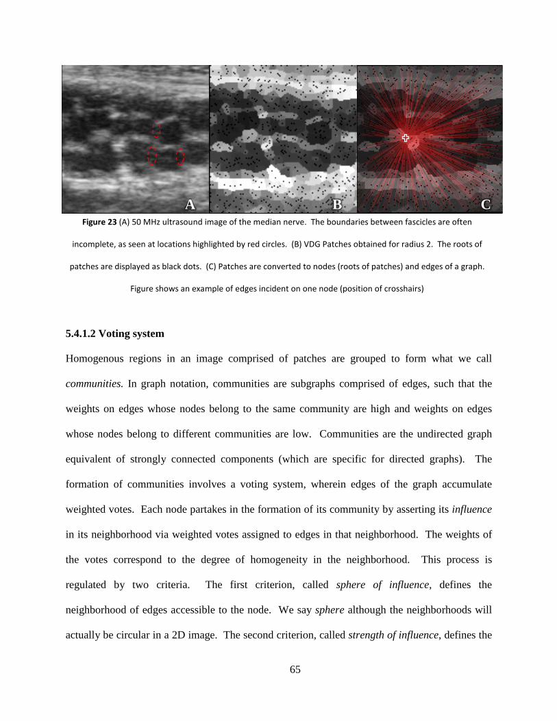
Figure 23 (A) 50 MHz ultrasound image of the median nerve. The boundaries between fascicles are often
incomplete, as seen at locations highlighted by red circles. (B) VDG Patches obtained for radius 2. The roots of
patches are displayed as black dots. (C) Patches are converted to nodes (roots of patches) and edges of a graph.
Figure shows an example of edges incident on one node (position of crosshairs)
5.4.1.2 Voting system
Homogenous regions in an image comprised of patches are grouped to form what we call
communities. In graph notation, communities are subgraphs comprised of edges, such that the
weights on edges whose nodes belong to the same community are high and weights on edges
whose nodes belong to different communities are low. Communities are the undirected graph
equivalent of strongly connected components (which are specific for directed graphs). The
formation of communities involves a voting system, wherein edges of the graph accumulate
weighted votes. Each node partakes in the formation of its community by asserting its influence
in its neighborhood via weighted votes assigned to edges in that neighborhood. The weights of
the votes correspond to the degree of homogeneity in the neighborhood. This process is
regulated by two criteria. The first criterion, called sphere of influence, defines the
neighborhood of edges accessible to the node. We say sphere although the neighborhoods will
actually be circular in a 2D image. The second criterion, called strength of influence, defines the
A B C
65
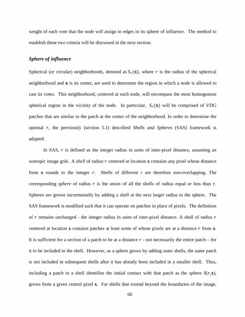
weight of each vote that the node will assign to edges in its sphere of influence. The method to
establish these two criteria will be discussed in the next section.
Sphere of influence
Spherical (or circular) neighborhoods, denoted as S𝑟𝑟(𝐱𝐱), where 𝑐𝑐 is the radius of the spherical
neighborhood and 𝐱𝐱 is its center, are used to determine the region in which a node is allowed to
cast its votes. This neighborhood, centered at each node, will encompass the most homogenous
spherical region in the vicinity of the node. In particular, S𝑟𝑟(𝐱𝐱) will be comprised of VDG
patches that are similar to the patch at the center of the neighborhood. In order to determine the
optimal 𝑐𝑐, the previously (section 5.1) described Shells and Spheres (SAS) framework is
adapted.
In SAS, 𝑐𝑐 is defined as the integer radius in units of inter-pixel distance, assuming an
isotropic image grid. A shell of radius 𝑐𝑐 centered at location x contains any pixel whose distance
from x rounds to the integer 𝑐𝑐. Shells of different r are therefore non-overlapping. The
corresponding sphere of radius 𝑐𝑐 is the union of all the shells of radius equal or less than 𝑐𝑐.
Spheres are grown incrementally by adding a shell at the next larger radius to the sphere. The
SAS framework is modified such that it can operate on patches in place of pixels. The definition
of 𝑐𝑐 remains unchanged - the integer radius in units of inter-pixel distance. A shell of radius 𝑐𝑐
centered at location x contains patches at least some of whose pixels are at a distance 𝑐𝑐 from x.
It is sufficient for a section of a patch to be at a distance 𝑐𝑐 - not necessarily the entire patch – for
it to be included in the shell. However, as a sphere grows by adding outer shells, the same patch
is not included in subsequent shells after it has already been included in a smaller shell. Thus,
including a patch in a shell identifies the initial contact with that patch as the sphere S(𝑐𝑐,x),
grows from a given central pixel x. For shells that extend beyond the boundaries of the image,
66

only pixels within the truncated shell are used. Thus, no assumption is made about the value of
pixels outside the image. A sphere of radius 𝑐𝑐 contains patches that are completely enclosed by
the sphere. Similar to the original SAS framework, spheres are grown incrementally by adding a
shell at the next larger radius to the sphere. Patches that are partially enclosed by the sphere are
either included in or excluded from the sphere of influence based on a decision criteria explained
below.
Figure 24 Synthetic isotropic image depicting the SAS framework applied to patches. A and B are two distinct
patches. Numbers assigned to pixels denotes inter-pixel distance from the central pixel x, denoted 0. The circle
denotes sphere Sr(x) where the radius r = 2.
To illustrate the new SAS framework, consider an image grid of isotropic pixels
comprising of two distinct patches labeled “A” and “B” (Figure 24). Numbers assigned to pixels
denotes inter-pixel radius from the pixel x at center of the image, where that radius is 0, and thus
identify their membership in that particular shell. The circle in Figure 24 denotes a sphere of
radius 2 formed by the union of shells of radius 0, 1, and 2. It can be seen that patch A is
completely enclosed in the sphere of radius 2 and hence, is included in the sphere. However,
67

patch B is only partially enclosed by the sphere, and its inclusion is determined using a decision
criteria described below.
The sphere at x can have a range of values for radius 𝑐𝑐 (up to some maximum 𝑐𝑐). A
particular 𝑐𝑐 is chosen by a method described in the next section, for the sphere of influence at x,
such that S𝑟𝑟(𝐱𝐱) will be the sphere centered at x whose radius causes it to contain the group of
patches whose homogeneity is high and becomes most inhomogeneous with the addition of the
next shell.
Identification of Sphere of influence and Strength of influence
The method used to identify the radius r of the sphere of influence S𝑟𝑟(𝐱𝐱), at a particular x and
the associated degree of influence, denoted as 𝑊𝑊S(𝐱𝐱), that a node can assign to the edges
between nodes in S𝑟𝑟(𝐱𝐱) will now be discussed. At each node in the graph, starting from radius
zero, spheres up to a predetermined maximum radius are evaluated (that maximum is chosen so
as to accommodate the expected size of any structure of interest). At each radius, the intensity
variance of a set of pixels including those within the sphere is computed. The set also includes
pixels outside the sphere from patches only partially within the sphere. This enhances the
change in variance when encountering a new patch. Computational efficiency is gained by
precomputing for each patch the sum S, sum of squared intensities Sq and the number of pixels Ñ
within each patch. Then, as each shell is added, variance is computed as
𝑉𝑉 = 𝑆𝑆𝑞𝑞 − (𝑆𝑆 ∗ 𝑆𝑆/Ñ)
Ñ − 1. 10
As the sphere grows, fractional change C in variance between two adjacent radii is computed.
68

𝐶𝐶 =|𝑉𝑉ℎ − 𝑉𝑉𝑙𝑙|
𝑉𝑉𝑙𝑙 11
where, 𝑉𝑉𝑙𝑙 and 𝑉𝑉ℎ are the variance in intensity within spheres at lower and higher radius
respectively. The sphere corresponding to the subjacent radius that generates the highest change
in variance is selected as S𝑟𝑟(𝐱𝐱), and the corresponding scalar value C is chosen as the weight of
influence 𝑊𝑊S(𝐱𝐱). Partially enclosed patches within S𝑟𝑟(𝐱𝐱) are then re-examined as described in
the next section.
Figure 25 shows the radius (represented by color) of S𝑟𝑟(𝐱𝐱) obtained at each node using
the method described above. Spheres up to a maximum radius of 14 (the maximum size of
potential targets) were evaluated.
Figure 25 Radius of 𝐒𝐒𝒓𝒓(𝐱𝐱) computed at each node using change in variance method.
69

Partially enclosed patches
Given the optimal radius 𝑐𝑐, the next question is which patches to actually include in the set
defined by the sphere of influence S𝑟𝑟(𝐱𝐱). That set of patches will not normally define a region
of pixels that is actually spherical, since individual patches may extend beyond the original
sphere of pixels. Thus we use the term sphere of influence in the sense that a country might have
one that is not geographically spherical. The patches in the sphere of influence S𝑟𝑟(𝐱𝐱) will be a
subset of the patches used to compute 𝑐𝑐. Patches that are completely enclosed in the sphere are
by default included. However, partially enclosed patches are reanalyzed to determine whether
they should be included in S𝑟𝑟(𝐱𝐱) by performing Fisher’s permutation test with the Student’s t-
test to assess the degree of homogeneity of the partially enclosed patch in relation to the
completely enclosed patches. Let P and Q be the intensity distribution functions of the partially
enclosed patch and the group of completely enclosed patches respectively. Let the samples in P
and Q be the N and M constituent pixels of the corresponding patches, p = (p1,p2,…,pN) and q =
(q1,q2,…,qM) respectively. The Student’s t-test is given by:
𝑡𝑡 =|𝑝 − 𝑞𝑞|
𝜎𝜎𝑃𝑃2𝑁𝑁 +
𝜎𝜎𝑄𝑄2𝑀𝑀
12
where, 𝑝 and 𝑞𝑞 are the sample means, and 𝜎𝜎𝑃𝑃and 𝜎𝜎𝑄𝑄are the standard deviations of P and Q. We
wish to test the null hypothesis H0 of no difference between P and Q, H0: P = Q. If the null
hypothesis is not true, we expect to observe larger values of 𝑡𝑡 than if H0 is true. Fisher’s
permutation testing allows us to run the hypothesis test without quantifying a fixed threshold for
t, but rather to have the threshold be determined by percentage of the population irrespective of
particular expected distribution. Thus non-Gaussian intensity populations are accommodated. To
perform the test, the samples p and q are pooled together. A sample (P*) of size N is obtained
70

from the pool without replacement (each sample only taken once) to represent P, and the
remaining M observations (Q*) then represents Q. The t-test (t*) is computed for P* and Q*,
and this process is repeated a large number of times (determined empirically). If the original t-
test falls above the η% of the distribution of t*, the permutation test rejects the null hypothesis at
η% level. Thus, η regulates the process of inclusion vs. exclusion of patches, especially for
borderline patches. Lower values of η, such as 0.1 or 1, favor exclusion, while higher values,
such as 5 or 10, favor inclusion. The permutation test is performed individually on each partially
enclosed patch at the particular radius of S𝑟𝑟(𝐱𝐱). For the example in Figure 24, for 𝑐𝑐=2, the
permutation test is performed for patch B (P in equation 12), with the completely enclosed patch
A (Q in equation 12). Patch B is included in 𝑆𝑆𝑟𝑟(x) only if H0 is accepted.
Casting and receiving votes
S𝑟𝑟(𝐱𝐱) and its associated 𝑊𝑊S(𝐱𝐱) are computed at each node of the graph, i.e., with x located at
the root of each patch. Since each S𝑟𝑟(𝐱𝐱) will include multiple distinct patches, each S𝑟𝑟(𝐱𝐱) also
encloses a subgraph of nodes and edges. The edges within a given S𝑟𝑟(𝐱𝐱), that is, between nodes
that are both within S𝑟𝑟(𝐱𝐱), receive votes equal to 𝑊𝑊S(𝐱𝐱). Spheres of influence of adjacent nodes
may overlap considerably, resulting in certain edges belonging to multiple spheres of influence
and thus receiving multiple votes. The total weight on an edge 𝑤𝑤𝒩𝒩𝑖𝑖,𝒩𝒩𝑗𝑗 is normalized by the
number constituent weights 𝑊𝑊S(𝐱𝐱) contributed by all the overlapping spheres that contain the
edge.
71
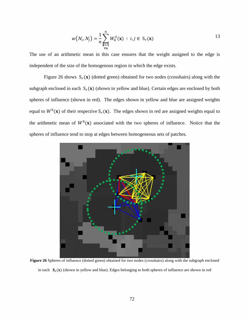
𝑤𝑤𝒩𝒩𝑖𝑖 ,𝒩𝒩𝑗𝑗 =1𝑖𝑖𝑊𝑊𝑘𝑘
𝑆𝑆(𝐱𝐱)𝑛𝑛
𝒌𝒌=𝟏𝟏∀𝐱𝐱
∶ 𝑖𝑖, 𝑗𝑗 ∈ S𝑟𝑟(𝐱𝐱) 13
The use of an arithmetic mean in this case ensures that the weight assigned to the edge is
independent of the size of the homogenous region in which the edge exists.
Figure 26 shows S𝑟𝑟(𝐱𝐱) (dotted green) obtained for two nodes (crosshairs) along with the
subgraph enclosed in each S𝑟𝑟(𝐱𝐱) (shown in yellow and blue). Certain edges are enclosed by both
spheres of influence (shown in red). The edges shown in yellow and blue are assigned weights
equal to 𝑊𝑊S(𝐱𝐱) of their respective S𝑟𝑟(𝐱𝐱). The edges shown in red are assigned weights equal to
the arithmetic mean of 𝑊𝑊S(𝐱𝐱) associated with the two spheres of influence. Notice that the
spheres of influence tend to stop at edges between homogeneous sets of patches.
Figure 26 Spheres of influence (dotted green) obtained for two nodes (crosshairs) along with the subgraph enclosed
in each 𝐒𝐒𝒓𝒓(𝐱𝐱) (shown in yellow and blue). Edges belonging to both spheres of influence are shown in red
72

Thus, each node asserts its influence, equal to the strength of the most prominent
boundary in its vicinity, on edges that connect nodes similar to itself. The collective influence of
all the nodes generates subsets of nodes whose edges within the subset have high connectivity.
We call such subsets of nodes “communities”. Figure 27 shows the graph structure obtained by
applying the above methods on the data shown in Figure 23A. Spheres were evaluated up to a
maximum radius of 14. Permutation testing for partially enclosed patches was carried out 10000
times and a threshold for inclusions/exclusion of partially enclosed patches set at η=0.1. The
color of the edge in Figure 27 represents the accumulated weight (color bar to the left). Edges
with weights equal to zero are not shown. As expected, while homogeneous regions contain
communities comprised of highly weighted edges, edges between heterogeneous patches are
either absent or low weighted. .
73
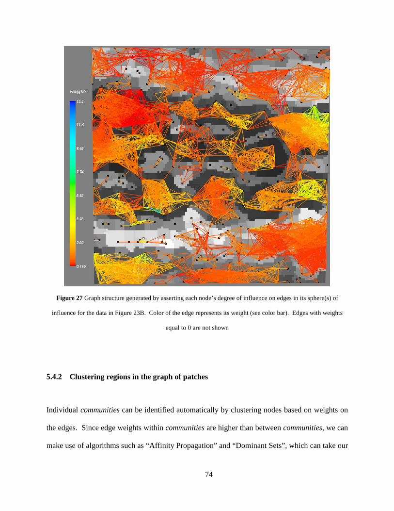
Figure 27 Graph structure generated by asserting each node’s degree of influence on edges in its sphere(s) of
influence for the data in Figure 23B. Color of the edge represents its weight (see color bar). Edges with weights
equal to 0 are not shown
5.4.2 Clustering regions in the graph of patches
Individual communities can be identified automatically by clustering nodes based on weights on
the edges. Since edge weights within communities are higher than between communities, we can
make use of algorithms such as “Affinity Propagation” and “Dominant Sets”, which can take our
74

weighted edges (Figure 28A) as input measures of similarity (affinity matrix), and can output
clusters of strongly connected nodes. In the next section, these two clustering algorithms are
discussed and results obtained by applying them to the graph structured created as described
above are shown.
5.4.2.1 Affinity propagation
Frey and Dueck (Frey & Dueck, 2007) have proposed a clustering algorithm, called affinity
propagation, that clusters data points (in our case, the nodes 𝒩𝒩 representing roots of patches) by
passing messages between them until a set of representative exemplars, each with a
corresponding cluster, emerge. There are two kinds of messages that are passed between data
points – the “responsibility” r(i,k) sent from data point i to candidate exemplar point k, and the
“availability” a(i,k) sent from candidate exemplar point k to data point i. These messages are
updated at each iteration of the algorithm according to the update equations:
𝑐𝑐(𝑖𝑖, 𝑘𝑘) ← 𝑤𝑤(𝑖𝑖,𝑘𝑘) − max𝑘𝑘′: 𝑘𝑘′≠𝑘𝑘
𝑎𝑎(𝑖𝑖,𝑘𝑘′) + 𝑤𝑤(𝑖𝑖, 𝑘𝑘′) 14
𝑎𝑎(𝑖𝑖,𝑘𝑘) ← min 0, 𝑐𝑐(𝑘𝑘,𝑘𝑘) + max 0, 𝑐𝑐(𝑖𝑖′,𝑘𝑘)𝑖𝑖′: 𝑖𝑖′∉𝑖𝑖,𝑘𝑘
15
𝑎𝑎(𝑘𝑘, 𝑘𝑘) ← max 0, 𝑐𝑐(𝑖𝑖′,𝑘𝑘)𝑖𝑖′: 𝑖𝑖′≠𝑘𝑘
16
where 𝑤𝑤 is the affinity matrix (the weights assigned to our edges), which holds the similarity
between data points 𝑖𝑖 and 𝑘𝑘. The diagonal elements 𝑤𝑤(𝑘𝑘,𝑘𝑘), called “preferences”, denote the
likelihood of data point 𝑘𝑘 to be chosen as the exemplar. All 𝑤𝑤(𝑘𝑘,𝑘𝑘) elements are set to a
common value, so that each data point is equally likely to be chosen as an exemplar. Setting the
preferences too low yields too few clusters, while setting it too high yields too many clusters. In
75

our case we set the preferences to the median of the all 𝑤𝑤(𝑖𝑖, 𝑗𝑗) elements, resulting in a moderate
number of clusters. To avoid numerical oscillations when updating messages, each message is
damped by setting it to a dampling value 𝜆𝜆 times its value from the previous iteration plus (1- 𝜆𝜆)
times its prescribed updated value. Unlike other clustering algorithms such as k-means that
require the number of clusters and seed points be pre-specified, affinity propagation starts by
considering all data points as potential exemplars and iteratively converges to meaningful
clusters.
The affinity matrix of communities was provided as input to the affinity propagation
algorithm. The damping factor 𝜆𝜆 was set to 0.5 and the algorithm was terminated either after 200
iterations or when the number of estimated clusters remained unchanged for 15 iterations. The
clusters that were generated are shown in Figure 28(B)
5.4.2.2 Dominant Sets
Like affinity propagation, dominant sets (Pavan & Pelillo, 2003) is another non-hierarchical
graph-theoretic iterative clustering framework that extends the notion of maximal clique to edge-
weighted graphs. A dominant set is a cluster of vertices/nodes S in an edge-weighted graph 𝐺𝐺 =
(𝒩𝒩,𝐸𝐸). S is a subset of 𝒩𝒩 (𝑆𝑆 ⊆ 𝒩𝒩), initially the “dominant” subset, in our case, an individual
community. The dominant set is removed from 𝐺𝐺, and the algorithm proceeds to the next
iteration to find the next community. The formal definition of a dominant set makes use of the
terms defined in equations 17-22. Given that 𝑖𝑖 ∈ 𝒩𝒩, and that the elements of the affinity matrix
of 𝐺𝐺 are denoted as 𝑤𝑤𝑖𝑖𝑗𝑗,
76

𝑎𝑎𝑤𝑤𝑑𝑑𝑖𝑖𝑎𝑎𝑆𝑆(𝑖𝑖) =1
|𝑆𝑆|𝑤𝑤𝑖𝑖𝑗𝑗𝑗𝑗∈𝑆𝑆
17
is the average of the weighted edges incident on node 𝑖𝑖 and the nodes in 𝑆𝑆, or in graph theory
parlance, the average weighted “degree of 𝑖𝑖 with respect to 𝑆𝑆.” The next term,
𝜙𝜙𝑆𝑆(𝑖𝑖, 𝑗𝑗) = 𝑤𝑤𝑖𝑖𝑗𝑗 − 𝑎𝑎𝑤𝑤𝑑𝑑𝑖𝑖𝑎𝑎𝑆𝑆(𝑖𝑖) ∶ 𝑗𝑗 ∉ 𝑆𝑆 18
measures the similarity between nodes 𝑖𝑖 and 𝑗𝑗, with respect to the average similarity between
node 𝑖𝑖 and its adjacent nodes in 𝑆𝑆. Now, let 𝑖𝑖 ∈ 𝑆𝑆. Then
𝜔𝜔𝑆𝑆(𝑖𝑖) = 1, 𝑖𝑖𝑖𝑖 |𝑆𝑆| = 1
𝜙𝜙𝑆𝑆\𝑖𝑖(𝑗𝑗, 𝑖𝑖) 𝜔𝜔𝑆𝑆\𝑖𝑖(𝑗𝑗),𝑗𝑗∈𝑆𝑆\𝑖𝑖
𝑐𝑐𝑡𝑡ℎ𝑖𝑖𝑐𝑐𝑤𝑤𝑖𝑖𝑖𝑖𝑖𝑖 19
transforms edge weights to weights on nodes for those nodes in 𝑆𝑆, such that, 𝜔𝜔𝑆𝑆(𝑖𝑖) measures the
similarity between node 𝑖𝑖 and the nodes of 𝑆𝑆\𝑖𝑖 with respect to the overall similarity among the
vertices in 𝑆𝑆\𝑖𝑖, thereby inducing a ranking of the nodes in S. The total weight of 𝑆𝑆 is given by
𝜳𝜳(𝑺𝑺) = 𝝎𝝎𝑺𝑺(𝒊𝒊)𝒊𝒊∈𝑺𝑺
20
We can now define a dominant set as a non-empty subset of vertices 𝑆𝑆 ⊆ 𝒩𝒩 such that 𝛹𝛹(𝑇𝑇) > 0
for any non-empty 𝑇𝑇 ⊆ 𝑆𝑆 under the conditions that 𝜔𝜔𝑆𝑆(𝑖𝑖) > 0,𝑖𝑖𝑐𝑐𝑐𝑐 𝑎𝑎𝑎𝑎𝑎𝑎 𝑖𝑖 ∈ 𝑆𝑆 and 𝜔𝜔𝑆𝑆∪𝑖𝑖(𝑖𝑖) <
0, 𝑖𝑖𝑐𝑐𝑐𝑐 𝑎𝑎𝑎𝑎𝑎𝑎 𝑖𝑖 ∉ 𝑆𝑆. The two conditions correspond to the properties of homogeneity within the
dominant set and inhomogeneity between them, respectively. The authors prove a tight
correspondence between the problem of finding dominant sets and that of finding solutions of a
quadratic program such as
77

𝐚𝐚𝐚𝐚𝐚𝐚𝐚𝐚𝐚𝐚𝐱𝐱 𝐱𝐱∈
𝟏𝟏𝟐𝟐𝐱𝐱𝐓𝐓𝑨𝑨𝐱𝐱 21
where = x ∈ ℝ𝑛𝑛 ∶ x ≥ 0 and 𝑖𝑖Tx = 1 is the standard simplex of ℝ𝑛𝑛, x is a vector belonging
to ℝ𝑛𝑛 , and 𝐴𝐴 is the affinity matrix. The solution to equation 21 is obtained using a continuous
optimization technique, called replicator dynamics, borrowed from evolutionary game theory.
The replicator equation in the discrete case is given by:
𝒙𝒙𝒊𝒊(𝒕𝒕 + 𝟏𝟏) = 𝒙𝒙𝒊𝒊(𝒕𝒕)(𝑨𝑨𝐱𝐱(𝒕𝒕))𝒊𝒊𝐱𝐱(𝒕𝒕)𝐓𝐓𝑨𝑨𝐱𝐱(𝒕𝒕)
22
where 𝐴𝐴 is the affinity matrix of 𝐺𝐺. Execution of the replicator dynamical system will result in a
dominant set (for more details, refer (Pavan & Pelillo, 2003)). The dominant set is removed
from the graph and replicator dynamics is run iteratively until all vertices have been clustered.
The clusters created by the dominant sets algorithm for the affinity matrix corresponding to the
communities in Figure 27 are shown in Figure 28(C). Similar to the results of affinity
propagation shown in Figure 28(B), the clusters consist of data points that are most
homogeneous to each other in their neighborhood.
78

Figure 28 Clusters obtained for the affinity matrix (A) by applying affinity propagation (B) and dominant sets (C)
algorithms.
5.4.3 Segmenting anatomical structures
As seen in the results of the patch clustering algorithms (Figure 28B and Figure 28C), the
resulting clusters accurately delineate homogeneous groups of patches, which we call fragments.
We are interested in detecting structures that are circular in at least one dimension, in particular,
individual roughly-cylindrical fascicles in the median nerve image. We accomplish this by
clustering fragments with a spherical shape prior. Accordingly, we introduce the final level in
the hierarchical graph structure, the segmentation, as shown as the top box in Figure 29.
A
B C
79

Figure 29 Our hierarchical graph structure for segmentation. Starting with pixels, each level is associated with a
graph whose nodes are data element resulting from the previous level.
Let ℒ𝑖𝑖 be the labels assigned to each fragment. The fragments and their representative
data points (exemplars in the case of affinity propagation and nodes with highest weight in each
cluster for dominant sets) may be modeled as a directed graph, G′ = (𝒩𝒩′, E′), with
representative data points forming the nodes (𝒩𝒩′). We assign a weight on a given edge
𝑤𝑤′(𝒩𝒩𝑖𝑖′,𝒩𝒩𝑗𝑗′), i.e., between two fragments, as the sum of the weights of all the edges crossing
between those two fragments (equation 23). Unlike the graph structure for the patches, wherein
the degree of each node is allowed to be greater than one, the outdegree of G’ is limited to 1;
each fragment points to only one other fragment, determined by the edge E′ with the highest 𝑤𝑤′
(equation 24).
80
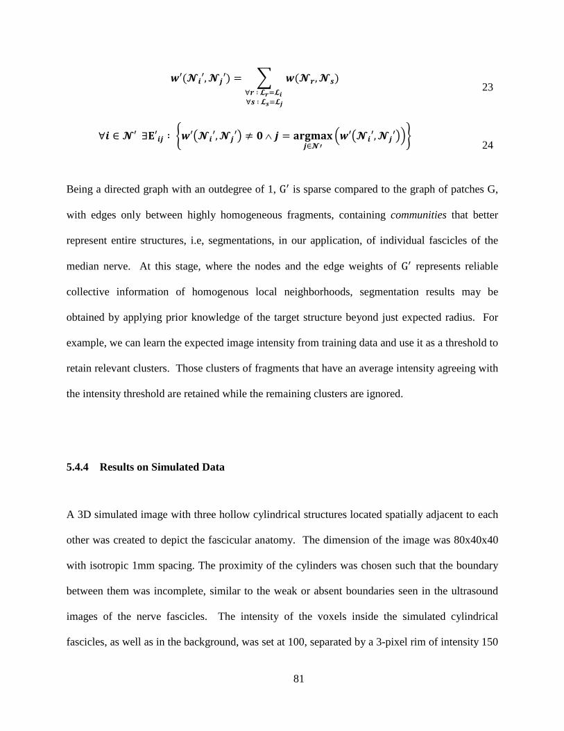
𝒘𝒘′(𝓝𝓝𝒊𝒊′,𝓝𝓝𝒋𝒋′) = 𝒘𝒘(𝓝𝓝𝒓𝒓,𝓝𝓝𝒔𝒔)∀𝒓𝒓 ∶ 𝓛𝓛𝒓𝒓=𝓛𝓛𝒊𝒊 ∀𝒔𝒔 ∶ 𝓛𝓛𝒔𝒔=𝓛𝓛𝒋𝒋
23
∀𝒊𝒊 ∈ 𝓝𝓝′ ∃𝐄𝐄′𝒊𝒊𝒋𝒋 ∶ 𝒘𝒘′𝓝𝓝𝒊𝒊′,𝓝𝓝𝒋𝒋′ ≠ 𝟎𝟎 ∧ 𝒋𝒋 = 𝐚𝐚𝐚𝐚𝐚𝐚𝐚𝐚𝐚𝐚𝐱𝐱𝒋𝒋∈𝓝𝓝′
𝒘𝒘′𝓝𝓝𝒊𝒊′,𝓝𝓝𝒋𝒋′ 24
Being a directed graph with an outdegree of 1, G′ is sparse compared to the graph of patches G,
with edges only between highly homogeneous fragments, containing communities that better
represent entire structures, i.e, segmentations, in our application, of individual fascicles of the
median nerve. At this stage, where the nodes and the edge weights of G′ represents reliable
collective information of homogenous local neighborhoods, segmentation results may be
obtained by applying prior knowledge of the target structure beyond just expected radius. For
example, we can learn the expected image intensity from training data and use it as a threshold to
retain relevant clusters. Those clusters of fragments that have an average intensity agreeing with
the intensity threshold are retained while the remaining clusters are ignored.
5.4.4 Results on Simulated Data
A 3D simulated image with three hollow cylindrical structures located spatially adjacent to each
other was created to depict the fascicular anatomy. The dimension of the image was 80x40x40
with isotropic 1mm spacing. The proximity of the cylinders was chosen such that the boundary
between them was incomplete, similar to the weak or absent boundaries seen in the ultrasound
images of the nerve fascicles. The intensity of the voxels inside the simulated cylindrical
fascicles, as well as in the background, was set at 100, separated by a 3-pixel rim of intensity 150
81

simulating the nerve sheath. Gaussian noise with zero mean μ was added to the image. The
standard deviation σ of the Gaussian was varied to generate four images having signal-to-noise
ratios (SNR) of 5, 10, 15, and 20db (Figure 30). In the following sections we evaluate the
application of our methods to this 3D simulated image, using a number of efficacy metrics.
Figure 30 Axial slice of a 3D image consisting of three cylinders representing nerve fascicles with a surrounding
sheath, located adjacent to each other such that the boundaries between them are incomplete. Gaussian noise is
added to generate images having SNR 5db (A), 10db (B), 15db (C), and 20db (D).
5.4.4.1 Community Distribution
The objective of the segmentation is to generate communities in the graph structure such that
weights on edges within each community are high and weights on edges across different
communities are low. In order to determine the efficacy of the formation of such communities,
we propose an analysis called community distribution. Let us consider a grayscale image
consisting of a background and a few foreground objects. Let us also consider a ground truth
segmentation image with distinct labels for each foreground object and the background. Let us
A B
C D
5 db 10 db
15 db 20 db
82

generate the graph structure using the voting scheme described above for the grayscale image.
With the ground truth image as reference, for every pair of nodes in the graph, the weight on the
edge connecting the nodes is accumulated in one of four bins depending on the ground truth label
that the node corresponds to. The four bins are as follows:
(1) Both the nodes belong to the same foreground object.
(2) Both the nodes belong to the background.
(3) The nodes belong to different foreground objects.
(4) One node belongs to a foreground object and the other belongs to the background.
Ideally, edges across heterogeneous regions or across different foreground objects should not
belong to any Sphere of influence. Therefore, such edges should not receive any votes. Thus, we
should expect bins 3 and 4 to remain empty, while bins 1 and 2 receive high weights.
Figure 31 Community distribution for the simulated images shown in Figure 30
Figure 31 shows the community distribution generated for the simulated images shown in
Figure 30. As expected, bins 1 and 2 have received most of the weights, even in the lowest SNR
0
0.05
0.1
0.15
0.2
0.25
0.3
20 15 10 5
Cum
ulat
ive
wei
ght
SNR (db)
SameTargetBackgroundDiffTargetsTar&Back
83

case of 5 db. In fact, bin 4 did not receive any weight (remained at 0) in all four SNR cases. Bin
3 addresses the condition of missing boundary between adjacent target structures. In all four
SNR cases, the weights in bin 1 are much higher than the weights in bin 3 and 4. Thus, this
experiment verifies the capability of the algorithm to generate the desired communities on
simulated data with noise.
5.4.4.2 Rand index
Another way to assess the efficacy of our segmentation is the Rand Index (Rand, 1971), which
computes a similarity measure between two clusterings by considering all pairs of samples and
counting pairs that are assigned in the same or different clusters in the predicted and true
clusterings. The index ranges from 0 to 1, where, a value close to 0.0 signifies random labeling
and a value of exactly 1.0 signifies the clusterings are identical. Table 1 shows the Rand Index
computed for the clusters obtained using the graph based segmentation method described in the
previous sections for the four simulated images shown in Figure 30. The result confirms the
accuracy of the method to assign distinct labels to target structures even in the case of missing
boundaries between adjacent structures.
Table 1 Rand Index computed for four images shown in Figure 30
SNR (db) Rand Index
20 1.0
15 1.0
10 0.97
5 0.95
84
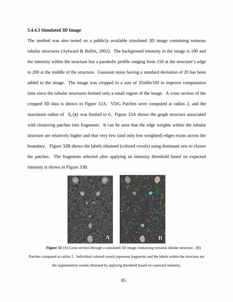
5.4.4.3 Simulated 3D Image
The method was also tested on a publicly available simulated 3D image containing tortuous
tubular structures (Aylward & Bullitt, 2002). The background intensity in the image is 100 and
the intensity within the structure has a parabolic profile ranging from 150 at the structure’s edge
to 200 at the middle of the structure. Gaussian noise having a standard deviation of 20 has been
added to the image. The image was cropped to a size of 35x66x100 to improve computation
time since the tubular structures formed only a small region of the image. A cross section of the
cropped 3D data is shown in Figure 32A. VDG Patches were computed at radius 2, and the
maximum radius of S𝑟𝑟(𝐱𝐱) was limited to 6. Figure 33A shows the graph structure associated
with clustering patches into fragments. It can be seen that the edge weights within the tubular
structure are relatively higher and that very few (and only low weighted) edges exists across the
boundary. Figure 32B shows the labels obtained (colored voxels) using dominant sets to cluster
the patches. The fragments selected after applying an intensity threshold based on expected
intensity is shown in Figure 33B.
Figure 32 (A) Cross section through a simulated 3D image containing tortuous tubular structure. (B)
Patches computed at radius 2. Individual colored voxels represent fragments and the labels within the structure are
the segmentation results obtained by applying threshold based on expected intensity.
A B
85
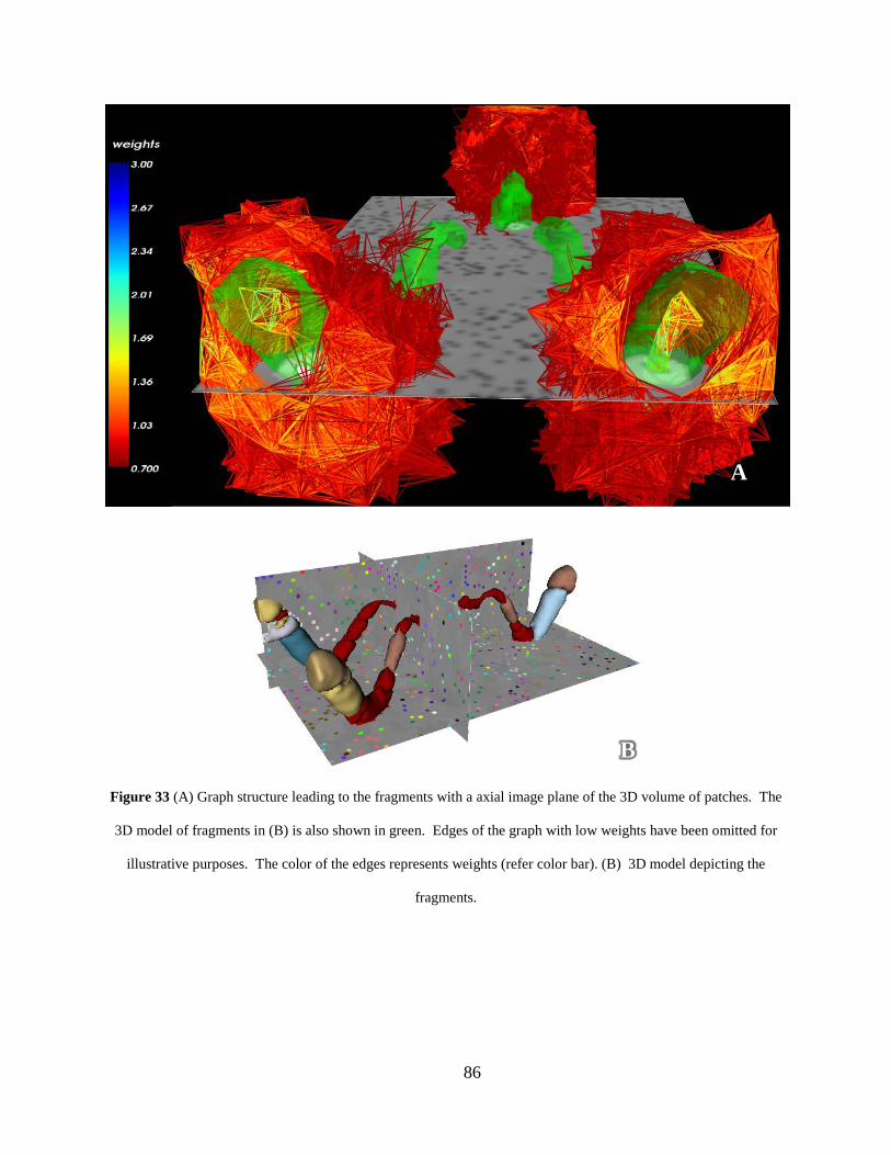
Figure 33 (A) Graph structure leading to the fragments with a axial image plane of the 3D volume of patches. The
3D model of fragments in (B) is also shown in green. Edges of the graph with low weights have been omitted for
illustrative purposes. The color of the edges represents weights (refer color bar). (B) 3D model depicting the
fragments.
A
B
86
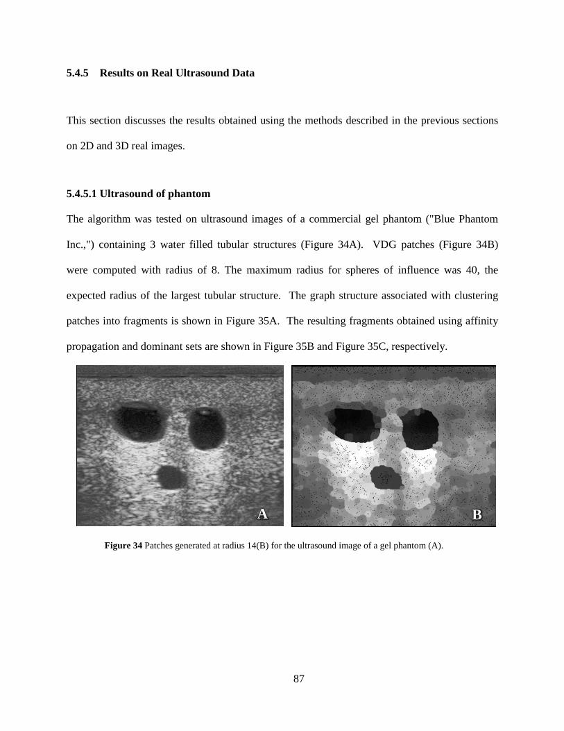
5.4.5 Results on Real Ultrasound Data
This section discusses the results obtained using the methods described in the previous sections
on 2D and 3D real images.
5.4.5.1 Ultrasound of phantom
The algorithm was tested on ultrasound images of a commercial gel phantom ("Blue Phantom
Inc.,") containing 3 water filled tubular structures (Figure 34A). VDG patches (Figure 34B)
were computed with radius of 8. The maximum radius for spheres of influence was 40, the
expected radius of the largest tubular structure. The graph structure associated with clustering
patches into fragments is shown in Figure 35A. The resulting fragments obtained using affinity
propagation and dominant sets are shown in Figure 35B and Figure 35C, respectively.
Figure 34 Patches generated at radius 14(B) for the ultrasound image of a gel phantom (A).
A B
87
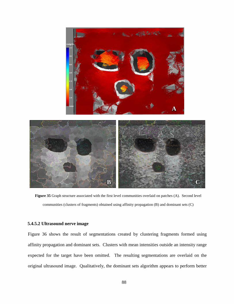
Figure 35 Graph structure associated with the first level communities overlaid on patches (A). Second level
communities (clusters of fragments) obtained using affinity propagation (B) and dominant sets (C)
5.4.5.2 Ultrasound nerve image
Figure 36 shows the result of segmentations created by clustering fragments formed using
affinity propagation and dominant sets. Clusters with mean intensities outside an intensity range
expected for the target have been omitted. The resulting segmentations are overlaid on the
original ultrasound image. Qualitatively, the dominant sets algorithm appears to perform better
A
B C
88
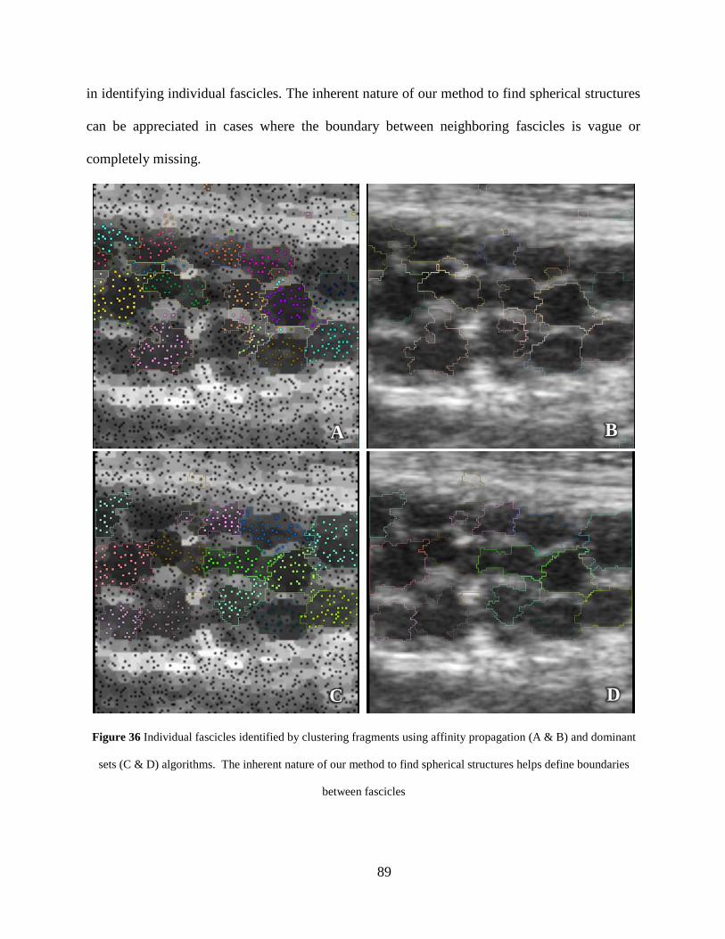
in identifying individual fascicles. The inherent nature of our method to find spherical structures
can be appreciated in cases where the boundary between neighboring fascicles is vague or
completely missing.
Figure 36 Individual fascicles identified by clustering fragments using affinity propagation (A & B) and dominant
sets (C & D) algorithms. The inherent nature of our method to find spherical structures helps define boundaries
between fascicles
A B
C D
89
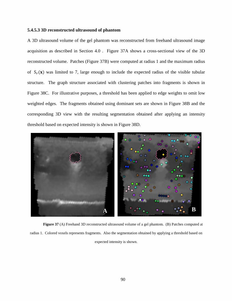
5.4.5.3 3D reconstructed ultrasound of phantom
A 3D ultrasound volume of the gel phantom was reconstructed from freehand ultrasound image
acquisition as described in Section 4.0 . Figure 37A shows a cross-sectional view of the 3D
reconstructed volume. Patches (Figure 37B) were computed at radius 1 and the maximum radius
of S𝑟𝑟(𝐱𝐱) was limited to 7, large enough to include the expected radius of the visible tubular
structure. The graph structure associated with clustering patches into fragments is shown in
Figure 38C. For illustrative purposes, a threshold has been applied to edge weights to omit low
weighted edges. The fragments obtained using dominant sets are shown in Figure 38B and the
corresponding 3D view with the resulting segmentation obtained after applying an intensity
threshold based on expected intensity is shown in Figure 38D.
Figure 37 (A) Freehand 3D reconstructed ultrasound volume of a gel phantom. (B) Patches computed at
radius 1. Colored voxels represents fragments. Also the segmentation obtained by applying a threshold based on
expected intensity is shown.
A B
90
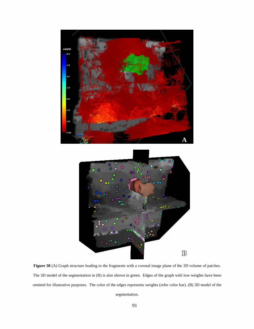
Figure 38 (A) Graph structure leading to the fragments with a coronal image plane of the 3D volume of patches.
The 3D model of the segmentation in (B) is also shown in green. Edges of the graph with low weights have been
omitted for illustrative purposes. The color of the edges represents weights (refer color bar). (B) 3D model of the
segmentation.
A
B
91

5.4.5.4 3D reconstructed ultrasound of the median nerve
A freehand 3D ultrasound volume of the median nerve was reconstructed using the same image
acquisition system described in the Section 4.0 . Patches were computed at radius 3 and the
maximum radius of S𝑟𝑟(𝐱𝐱) was limited to 12, large enough to include the expected radius of the
largest fascicle. The graph structure associated with clustering patches into fragments is shown in
Figure 40A along with a cross-sectional 2D slice. For illustrative purposes, a threshold has been
applied to edge weights to omit low weighted edges. The color of the edges represents weights
(refer color bar). The fragments obtained using dominant sets overlaid on a cross-sectional slice
of the patches are shown in Figure 39. Figure 40B is the resulting segmentation obtained after
applying an intensity threshold based on expected intensity, and the corresponding 3D model of
the segmentation result with a cross-sectional image plane is shown in Figure 41.
Figure 39 Cross-sectional view of patches computed at radius 3. Colored voxels represents fragments.
Also the segmentation obtained by applying a threshold based on expected intensity is shown.
92
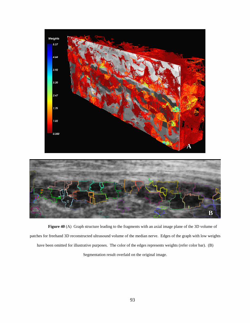
Figure 40 (A) Graph structure leading to the fragments with an axial image plane of the 3D volume of
patches for freehand 3D reconstructed ultrasound volume of the median nerve. Edges of the graph with low weights
have been omitted for illustrative purposes. The color of the edges represents weights (refer color bar). (B)
Segmentation result overlaid on the original image.
A
B
93
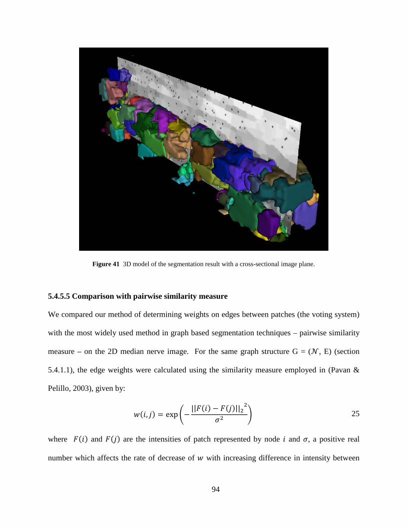
Figure 41 3D model of the segmentation result with a cross-sectional image plane.
5.4.5.5 Comparison with pairwise similarity measure
We compared our method of determining weights on edges between patches (the voting system)
with the most widely used method in graph based segmentation techniques – pairwise similarity
measure – on the 2D median nerve image. For the same graph structure G = (𝒩𝒩, E) (section
5.4.1.1), the edge weights were calculated using the similarity measure employed in (Pavan &
Pelillo, 2003), given by:
𝑤𝑤(𝑖𝑖, 𝑗𝑗) = exp −||𝐹𝐹(𝑖𝑖) − 𝐹𝐹(𝑗𝑗)||2
2
𝜎𝜎2 25
where 𝐹𝐹(𝑖𝑖) and 𝐹𝐹(𝑗𝑗) are the intensities of patch represented by node 𝑖𝑖 and 𝜎𝜎, a positive real
number which affects the rate of decrease of 𝑤𝑤 with increasing difference in intensity between
94
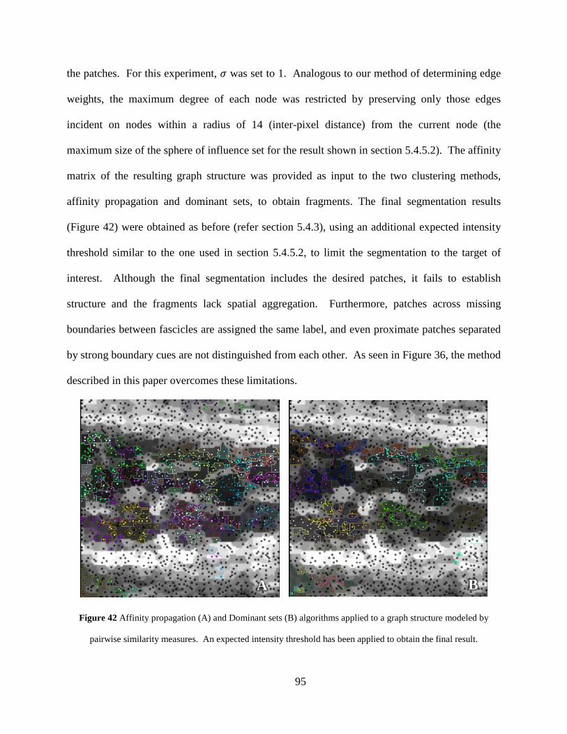
the patches. For this experiment, 𝜎𝜎 was set to 1. Analogous to our method of determining edge
weights, the maximum degree of each node was restricted by preserving only those edges
incident on nodes within a radius of 14 (inter-pixel distance) from the current node (the
maximum size of the sphere of influence set for the result shown in section 5.4.5.2). The affinity
matrix of the resulting graph structure was provided as input to the two clustering methods,
affinity propagation and dominant sets, to obtain fragments. The final segmentation results
(Figure 42) were obtained as before (refer section 5.4.3), using an additional expected intensity
threshold similar to the one used in section 5.4.5.2, to limit the segmentation to the target of
interest. Although the final segmentation includes the desired patches, it fails to establish
structure and the fragments lack spatial aggregation. Furthermore, patches across missing
boundaries between fascicles are assigned the same label, and even proximate patches separated
by strong boundary cues are not distinguished from each other. As seen in Figure 36, the method
described in this paper overcomes these limitations.
Figure 42 Affinity propagation (A) and Dominant sets (B) algorithms applied to a graph structure modeled by
pairwise similarity measures. An expected intensity threshold has been applied to obtain the final result.
A B
95

6.0 IMAGE REGISTRATION
An overview of image registration was presented in section 2.2.5.2. In this section, a hybrid atlas
based registration method that makes use of intensity corrections induced at anatomical
landmarks to regulate deformable intensity registration is presented. The developed method is
tested on the segmentation of the hippocampus in MRI images of brain and validated using
manual segmentations. Results show that our method agrees better with manual segmentations
than previously reported methods and other popular methods such as FIRST (M. Chen, Kanade,
Pomerleau, & Schneider, 1999) and FreeSurfer (Fischl et al., 2002).
In atlas based segmentation, a reference image, called as an atlas, in which structures of
interest have been manually segmented, is registered to the subject image under investigation.
The resulting spatial transformation maps the manual segmentation from the atlas coordinate
space to the subject coordinate space, yielding the resultant segmentation. The accuracy of the
final segmentation is conditional upon the image registration process, i.e., the accuracy of the
image-to-image correspondence in the region of interest. Methods that use global mapping
models, which take into account every voxel of the image in its cost function, are suitable for
applications like tissue (gray matter (GM), white matter (WM), and cerebrospinal liquid CSF)
segmentation in MR images of the brain, where the region of interest includes most of the image
voxels. However, in instances that involve local deformations, or when the region of interest
96

consists of a small volume of the image, global mapping models does not produce satisfactory
results because local distortions are averaged out equally over the entire image.
6.1 HYBRID LANDMARK-INTENSITY BASED REGISTRATION
We present a method (Figure 43) that applies local constraints to any intensity-based registration
algorithm. The local constraints, enforced as small neighborhoods of altered image intensity
around landmarks, holds fast predefined correspondences, while the registration algorithm finds
correspondence in rest of the image. This method can be applied to segment any structure in any
imaging modality. In this paper, we focus on the segmentation of the hippocampus in 7T MR
images of the brain.
Figure 43 Pipeline of the hybrid registration method
Subject
Identify Landmarks
Linear landmark registration
Non-linear landmark registration
Modify image with Ƒ
Deformable intensity-based
registration
Atlas
Apply deformation field
Man
ual S
egm
enta
tion
97

6.1.1 Methodology
6.1.1.1 Identify Landmarks
Landmarks are a set of discrete points in an image that are biologically homologous across all the
images in the dataset. Landmarks can be obtained either prior to the image acquisition, by
positioning physical fiducial markers at predetermined locations on the patient, or post image
acquisition, by deriving spatial locations in the images with the help of either sophisticated
image analysis tools or the knowledge of an expert. A set of six landmarks (Figure 44) were
identified in the hippocampus by an expert in the atlas and subject images using an image
analysis and visualization tool (Fedorov et al., 2012; "http://www.slicer.org,"). The protocol
provided in (Pluta et al., 2009) was followed to identify the landmarks. This process took
approximately 5 - 10 minutes for each subject depending on amount of deformation in the
hippocampus
Figure 44 (1-4) Sagittal view of MR image of brain showing the positioning of six landmarks (A-F). (5) 3D view
showing the six landmarks with axial and sagittal slices in the background
6.1.1.2 Landmark Registration
The goal of landmark registration is to find the transformation that maps the landmarks in the
atlas to the landmarks in the subject images. Let 𝑥𝑥𝐴𝐴𝑗𝑗 , and 𝑥𝑥𝑆𝑆
𝑗𝑗 , denote the spatial location of the jth
landmark in the atlas A and the subject S, respectively, j = 1,…, 𝑚𝑚, where 𝑚𝑚 ∈ ℕ denotes the
1 2 3 4 5
98
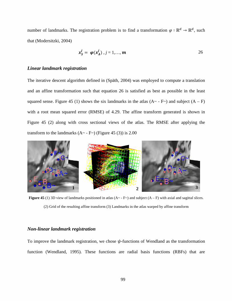
number of landmarks. The registration problem is to find a transformation 𝜑𝜑 ∶ ℝ𝑑𝑑 → ℝ𝑑𝑑, such
that (Modersitzki, 2004)
𝒙𝒙𝑺𝑺𝒋𝒋 = 𝝋𝝋(𝒙𝒙𝑨𝑨
𝒋𝒋 ) , j = 1,…, 𝒎𝒎 26
Linear landmark registration
The iterative descent algorithm defined in (Späth, 2004) was employed to compute a translation
and an affine transformation such that equation 26 is satisfied as best as possible in the least
squared sense. Figure 45 (1) shows the six landmarks in the atlas (A~ - F~) and subject (A – F)
with a root mean squared error (RMSE) of 4.29. The affine transform generated is shown in
Figure 45 (2) along with cross sectional views of the atlas. The RMSE after applying the
transform to the landmarks (A~ - F~) (Figure 45 (3)) is 2.00
Figure 45 (1) 3D view of landmarks positioned in atlas (A~ - F~) and subject (A – F) with axial and sagittal slices.
(2) Grid of the resulting affine transform (3) Landmarks in the atlas warped by affine transform
Non-linear landmark registration
To improve the landmark registration, we chose 𝜓𝜓-functions of Wendland as the transformation
function (Wendland, 1995). These functions are radial basis functions (RBFs) that are
1 3 2
99
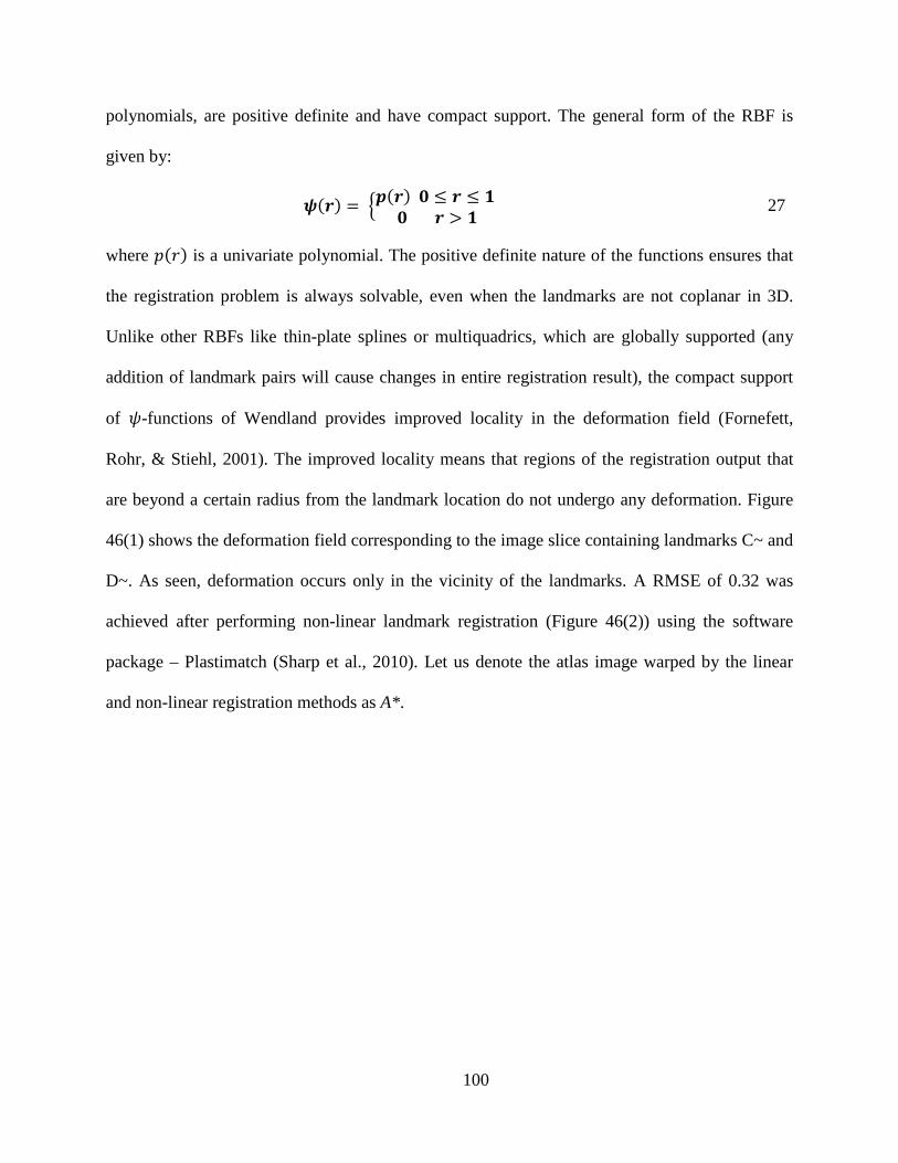
polynomials, are positive definite and have compact support. The general form of the RBF is
given by:
𝝍𝝍(𝒓𝒓) = 𝒑𝒑(𝒓𝒓) 𝟎𝟎 ≤ 𝒓𝒓 ≤ 𝟏𝟏 𝟎𝟎 𝒓𝒓 > 𝟏𝟏
27
where 𝑝𝑝(𝑐𝑐) is a univariate polynomial. The positive definite nature of the functions ensures that
the registration problem is always solvable, even when the landmarks are not coplanar in 3D.
Unlike other RBFs like thin-plate splines or multiquadrics, which are globally supported (any
addition of landmark pairs will cause changes in entire registration result), the compact support
of 𝜓𝜓-functions of Wendland provides improved locality in the deformation field (Fornefett,
Rohr, & Stiehl, 2001). The improved locality means that regions of the registration output that
are beyond a certain radius from the landmark location do not undergo any deformation. Figure
46(1) shows the deformation field corresponding to the image slice containing landmarks C~ and
D~. As seen, deformation occurs only in the vicinity of the landmarks. A RMSE of 0.32 was
achieved after performing non-linear landmark registration (Figure 46(2)) using the software
package – Plastimatch (Sharp et al., 2010). Let us denote the atlas image warped by the linear
and non-linear registration methods as A*.
100
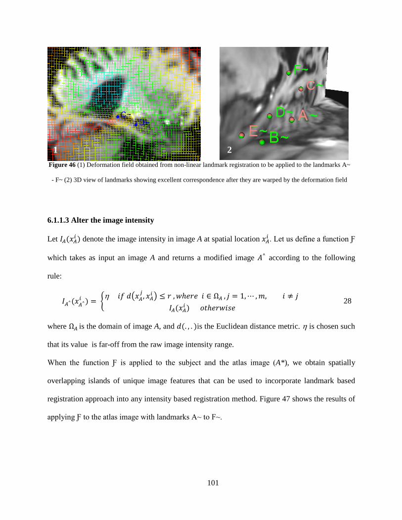
Figure 46 (1) Deformation field obtained from non-linear landmark registration to be applied to the landmarks A~
- F~ (2) 3D view of landmarks showing excellent correspondence after they are warped by the deformation field
6.1.1.3 Alter the image intensity
Let 𝐼𝐼𝐴𝐴(𝑥𝑥𝐴𝐴𝑖𝑖 ) denote the image intensity in image A at spatial location 𝑥𝑥𝐴𝐴𝑖𝑖 . Let us define a function Ƒ
which takes as input an image A and returns a modified image 𝐴𝐴^ according to the following
rule:
𝐼𝐼𝐴𝐴^(𝑥𝑥𝐴𝐴^𝑖𝑖 ) = η 𝑖𝑖𝑖𝑖 𝑑𝑑𝑥𝑥𝐴𝐴
𝑗𝑗 , 𝑥𝑥𝐴𝐴𝑖𝑖 ≤ 𝑐𝑐 ,𝑤𝑤ℎ𝑖𝑖𝑐𝑐𝑖𝑖 𝑖𝑖 ∈ Ω𝐴𝐴 , 𝑗𝑗 = 1,⋯ ,𝑚𝑚, 𝑖𝑖 ≠ 𝑗𝑗 𝐼𝐼𝐴𝐴(𝑥𝑥𝐴𝐴𝑖𝑖 ) 𝑐𝑐𝑡𝑡ℎ𝑖𝑖𝑐𝑐𝑤𝑤𝑖𝑖𝑖𝑖𝑖𝑖
28
where Ω𝐴𝐴 is the domain of image A, and 𝑑𝑑(. , . )is the Euclidean distance metric. η is chosen such
that its value is far-off from the raw image intensity range.
When the function Ƒ is applied to the subject and the atlas image (A*), we obtain spatially
overlapping islands of unique image features that can be used to incorporate landmark based
registration approach into any intensity based registration method. Figure 47 shows the results of
applying Ƒ to the atlas image with landmarks A~ to F~.
1 2
101
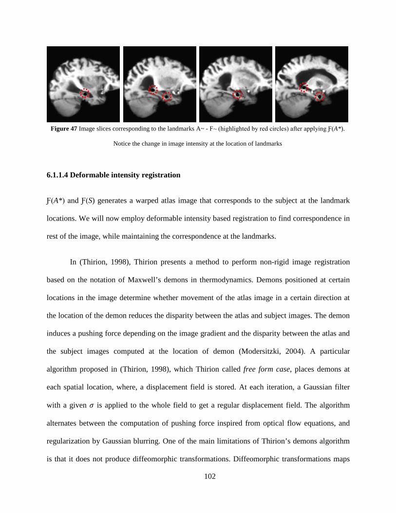
Figure 47 Image slices corresponding to the landmarks A~ - F~ (highlighted by red circles) after applying Ƒ(A*).
Notice the change in image intensity at the location of landmarks
6.1.1.4 Deformable intensity registration
Ƒ(A*) and Ƒ(S) generates a warped atlas image that corresponds to the subject at the landmark
locations. We will now employ deformable intensity based registration to find correspondence in
rest of the image, while maintaining the correspondence at the landmarks.
In (Thirion, 1998), Thirion presents a method to perform non-rigid image registration
based on the notation of Maxwell’s demons in thermodynamics. Demons positioned at certain
locations in the image determine whether movement of the atlas image in a certain direction at
the location of the demon reduces the disparity between the atlas and subject images. The demon
induces a pushing force depending on the image gradient and the disparity between the atlas and
the subject images computed at the location of demon (Modersitzki, 2004). A particular
algorithm proposed in (Thirion, 1998), which Thirion called free form case, places demons at
each spatial location, where, a displacement field is stored. At each iteration, a Gaussian filter
with a given 𝜎𝜎 is applied to the whole field to get a regular displacement field. The algorithm
alternates between the computation of pushing force inspired from optical flow equations, and
regularization by Gaussian blurring. One of the main limitations of Thirion’s demons algorithm
is that it does not produce diffeomorphic transformations. Diffeomorphic transformations maps
102

one differentiable manifold to another, such that both the transformation and its inverse are
smooth. Diffeomorphism is a requirement because these transformations preserve topology and
prevent cracks or folds of objects. In (Vercauteren, Pennec, Perchant, & Ayache, 2007), T.
Vercauteren et al have developed an efficient non-parametric diffeomorphic image registration
method as an extension to Thirion’s demons registration (Thirion, 1998).
Given a fixed image 𝐹𝐹(. ) and a moving image 𝑀𝑀(. ), let 𝑖𝑖(. ), 𝑝𝑝 → 𝑖𝑖(𝑝𝑝) be the
transformation that models the spatial mappings of points from fixed image space to moving
image space. Mean squared error is used as the similarity criterion 𝑆𝑆𝑖𝑖𝑚𝑚(. , . ), which measures
the resemblance of two images.
𝑺𝑺𝒊𝒊𝒎𝒎(𝑭𝑭,𝑴𝑴 𝒐𝒐 𝒔𝒔) = 𝟏𝟏
𝟐𝟐|Ω𝑷𝑷| |𝑭𝑭(𝒑𝒑) −𝑴𝑴(𝒔𝒔(𝒑𝒑)|𝟐𝟐𝒑𝒑∈Ω𝑷𝑷
29
where Ω𝑃𝑃 is the region of overlap between 𝐹𝐹 and 𝑀𝑀 𝑐𝑐 𝑖𝑖
Non-parametric image registration is treated as an optimization problem that aims at minimizing
a global energy (Vercauteren et al., 2007):
𝐸𝐸(𝑐𝑐, 𝑖𝑖) = 1𝜎𝜎𝑖𝑖2
𝑆𝑆𝑖𝑖𝑚𝑚(𝐹𝐹,𝑀𝑀 𝑐𝑐 𝑐𝑐) + 1𝜎𝜎𝑚𝑚2
𝑑𝑑𝑖𝑖𝑖𝑖𝑡𝑡(𝑖𝑖, 𝑐𝑐)2 + 1𝜎𝜎𝑇𝑇2
𝑅𝑅𝑖𝑖𝑎𝑎(𝑖𝑖) 30
where 𝑐𝑐 is a vector field that represents point correspondences between pixels, 𝑑𝑑𝑖𝑖𝑖𝑖𝑡𝑡(𝑖𝑖, 𝑐𝑐) =
||𝑐𝑐 − 𝑖𝑖||, 𝑅𝑅𝑖𝑖𝑎𝑎(𝑖𝑖) is the regularization criterion given by ||∇𝑖𝑖||2, and 𝜎𝜎𝑚𝑚 accounts for special
uncertainty on the correspondences.
Unlike Thirion’s demons algorithm, which registers the fixed and moving images by
optimizing equation 30 over the entire space of displacement fields, T. Vercauteren et al have
developed an alternate optimization scheme of the demons and combined it with Newton’s
method tools for Lie groups to provide free-form diffeomorphic transformations.
103

Figure 48 shows the deformation field corresponding to image slice containing
previously positioned landmarks E~ and F~ obtained using ITK implementation of T.
Vercauteren’s method (Johnson & Zhao, 2009). While the algorithm generates deformation
throughout the image, it is clearly seen that the deformation occurring in the vicinity of the
previously positioned landmarks (highlighted by red circle) is restricted by the islands of image
features generated using Ƒ, thereby, preserving previously achieved correspondences.
Figure 48 Deformation field obtained from demons warp for slice corresponding to landmarks E~ and F~ shown
in Figure 46
6.2 VALIDATION ON HIPPOCAMPUS SEGMENTATION
As mentioned earlier, the hybrid method presented in this dissertation was evaluated on the task
of segmentation of the hippocampus in MR images of the brain. The dataset consisted of 7T MR
104

images of seven subjects. The images were of dimensions 240 x 320 x 256 and 0.7mm isotropic
spacing. The right hippocampus was manually segmented for each subject and was used to
validate the results.
Preprocessing
The images were ACPC-aligned and the skulls were stripped using the Brain Extraction Tool
(BET) (Smith, 2002). Bias field correction was applied using the ITK (Ibanez, Schroeder, Ng, &
Cates, 2003) implementation of the non-uniform intensity normalization approach (Sled,
Zijdenbos, & Evans, 1998). The images were cropped to remove slices with no anatomical
information and normalized.
6.2.1 Comparison with previous similar methods
Figure 49 shows the overlap measures (O), defined below, for our method in comparison to the
measures reported in (Carmichael et al., 2005).
𝑂𝑂 = 2|𝐴𝐴 ∩𝑀𝑀|
|𝐴𝐴| + |𝑀𝑀| 31
where 𝐴𝐴and 𝑀𝑀are automated and manual segmentation volumes.
In (Carmichael et al., 2005), Carmichael et al compared the performance of the following
atlas based segmentation methods for hippocampus segmentation: AIR, SPM, FLIRT, and a fully
deformable method of Chen (M. Chen et al., 1999; Friston et al., 1995; Jenkinson, Bannister,
Brady, & Smith, 2002; Woods, Grafton, Holmes, Cherry, & Mazziotta, 1998). They reported
that Chen’s fully deformable method generated the highest overlap ratio (between 0.18 and 0.65
with median value 0.42) than the other methods. As seen in Figure 49, overlap measures
105
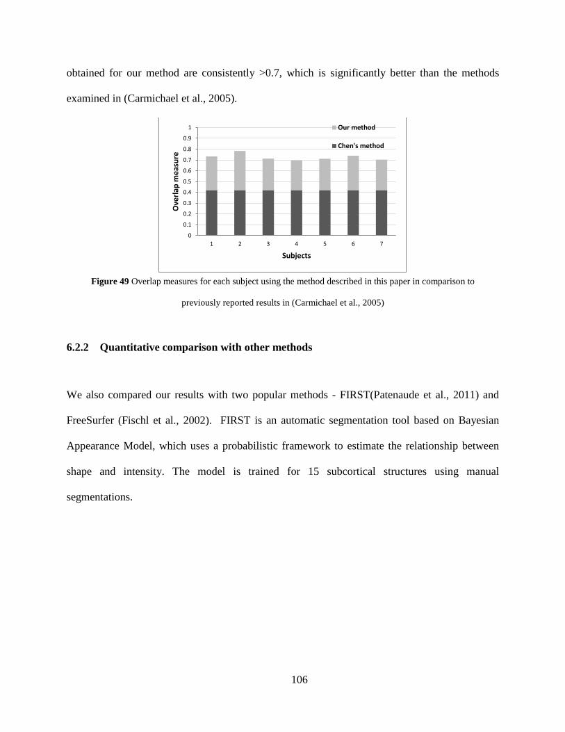
obtained for our method are consistently >0.7, which is significantly better than the methods
examined in (Carmichael et al., 2005).
Figure 49 Overlap measures for each subject using the method described in this paper in comparison to
previously reported results in (Carmichael et al., 2005)
6.2.2 Quantitative comparison with other methods
We also compared our results with two popular methods - FIRST(Patenaude et al., 2011) and
FreeSurfer (Fischl et al., 2002). FIRST is an automatic segmentation tool based on Bayesian
Appearance Model, which uses a probabilistic framework to estimate the relationship between
shape and intensity. The model is trained for 15 subcortical structures using manual
segmentations.
0
0.1
0.2
0.3
0.4
0.5
0.6
0.7
0.8
0.9
1
1 2 3 4 5 6 7
Ove
rlap
mea
sure
Subjects
Our method
Chen's method
106

Figure 50 Cross-sectional sagittal views of the segmentation results of FreeSurfer (row A), FIRST (row B), our
method (row C), and manual segmentation (row D). The false positives, indicated by red circles, are significantly
higher in both FIRST and FreeSurfer.
FreeSurfer is an image analysis suite that generates volumetric segmentations of subcortical
structures. It assigns a label to each location on a cortical surface model based on probabilistic
information estimated from a manually labeled training set. Figure 50 shows four cross-sectional
sagittal views of the segmentation results of FreeSurfer (row A), FIRST (row B), and our method
(row C). Figure 50 (row D) shows the manual segmentation for the corresponding slices. The
output of FreeSurfer appears in a different view since it converts the images to Talairach
107

coordinates. By analyzing the results qualitatively, it can be seen that the segmentation resulting
from our method concurs better than FIRST or FreeSurfer. It should be noted that false positives
are significantly higher in both FIRST and FreeSurfer. Quantitative comparison of the
hippocampus measures is not feasible since the tracing protocols used to generate the training
sets in FIRST and FreeSurfer differ from each other and also from the protocol used by us to
generate ground truth. Hence, the definition and geometry of the hippocampus formation will
vary across different methods, thereby, voiding any quantitative comparisons.
108
7.0 SIMULTANEOUS VISUALIZATION
A longitudinal study often involves examination and analysis of structural and/or functional
changes of a specific structure in the same patient over a period of time. Among other outcomes,
it provides physicians reliable data to interpret the patient’s response to treatment, and facilitates
the determination of subsequent treatment. Structural changes over a period of time can be
observed by correlating images of the structure that were acquired at different points in time. In
order to correlate multiple volumetric images, it is imperative to isolate the appropriate slice
corresponding to the structure of interest in each and every volume, which will likely be
laborious, analogous to finding needles in multiple haystacks, considering volumes are usually
comprised of hundreds of slices. Furthermore, as the structure of interest can span across more
than one slice in the image, examining the whole structure will involve analyzing multiple slices
simultaneously. As a result, correlation across multiple volumes will be even more tedious
because each time the operator selects a different slice, the corresponding slice in every other
volume should be identified manually. Correlation across multiple modalities can present
additional challenges since the same structure can appear differently in different modalities, thus
making identification of corresponding slices even more difficult. The entire process would
benefit greatly if the identification of corresponding slices could be performed automatically and
if doctors could concurrently visualize the corresponding anatomy registered automatically from
109

previous acquisitions while performing the current scan, thereby enabling them to perform
dynamic correlations.
In the following sections, we present methods that address the aforementioned
challenges. Foremost, the multiple volumetric images are registered to a single standard image
space, as described in section 7.1. Image slices from multiple volumes that correspond to the
same anatomical location will be displayed concurrently under two scenarios: offline (see
sections 7.2), and real-time (see section 7.3).
7.1 REGISTRATION OF PRIOR AND ACQUIRED VOLUMES
Often, medical images from more than one imaging modality are used to provide effective
medical care, since the drawbacks of one imaging modality can be balanced by another. For
example, MR and ultrasound imaging, employed for a particular application, can complement
each other well. MR images provide high resolution, low noise, and high contrast images of soft
tissue, but is very expensive and require substantial amount of time to acquire. In contrast,
ultrasound is low cost and real time, but highly noisy and not very reliable at differentiating soft
tissue types. Hence, an efficient approach would be to acquire MR images at only critical stages
of treatment and employ ultrasound for routine follow up studies. Another example of applying
multi-modality imaging is image guided surgery, wherein CT/MR images are generally used
only in pre-surgical planning, while ultrasound is used during surgery for guidance.
A critical step in the application of multi-modality imaging is finding anatomical
correspondence between the different images. Correspondence can be achieved by image
registration, as described in section 2.2.5.2. In this dissertation, prior volume (CT/MRI), and the
110
3D reconstructed ultrasound volumes acquired at different time points are registered to a single
standard image space using landmark registration described in section 6.1.1.2.
7.2 OFFLINE SIMULTANEOUS VISUALIZATION
In the offline mode, the coordinate system of the prior volume, e.g., the first ultrasound volume
that is acquired, is chosen as the standard image space to which all other volumes are registered.
Volumes in the standard space are loaded and linked in the 3D Slicer volumes module, such that,
moving through image slices in one volume will automatically display corresponding image
slices from the other volumes. At any given time, slices from up to 3 volumes and any binary
segmentation can be visualized simultaneously (Figure 51). For each volume, an image plane of
any arbitrary orientation may be visualized. Having the ability to visualize side-by-side the
corresponding slices from volumes acquired at different instances of time, physicians will be in a
better position to quantify and monitor changes in anatomical structures. Users can also make
measurements and add annotations to the images using the annotations module in 3D Slicer, and
these annotations transfer to the other images.
111
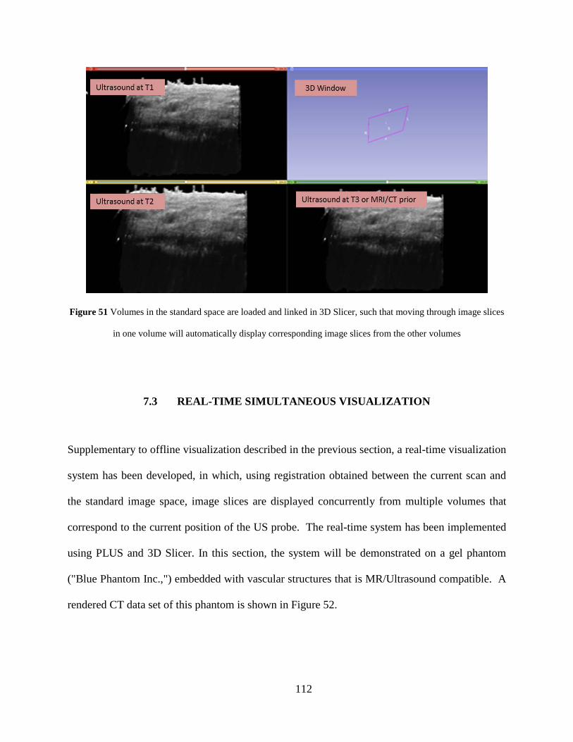
Figure 51 Volumes in the standard space are loaded and linked in 3D Slicer, such that moving through image slices
in one volume will automatically display corresponding image slices from the other volumes
7.3 REAL-TIME SIMULTANEOUS VISUALIZATION
Supplementary to offline visualization described in the previous section, a real-time visualization
system has been developed, in which, using registration obtained between the current scan and
the standard image space, image slices are displayed concurrently from multiple volumes that
correspond to the current position of the US probe. The real-time system has been implemented
using PLUS and 3D Slicer. In this section, the system will be demonstrated on a gel phantom
("Blue Phantom Inc.,") embedded with vascular structures that is MR/Ultrasound compatible. A
rendered CT data set of this phantom is shown in Figure 52.
112
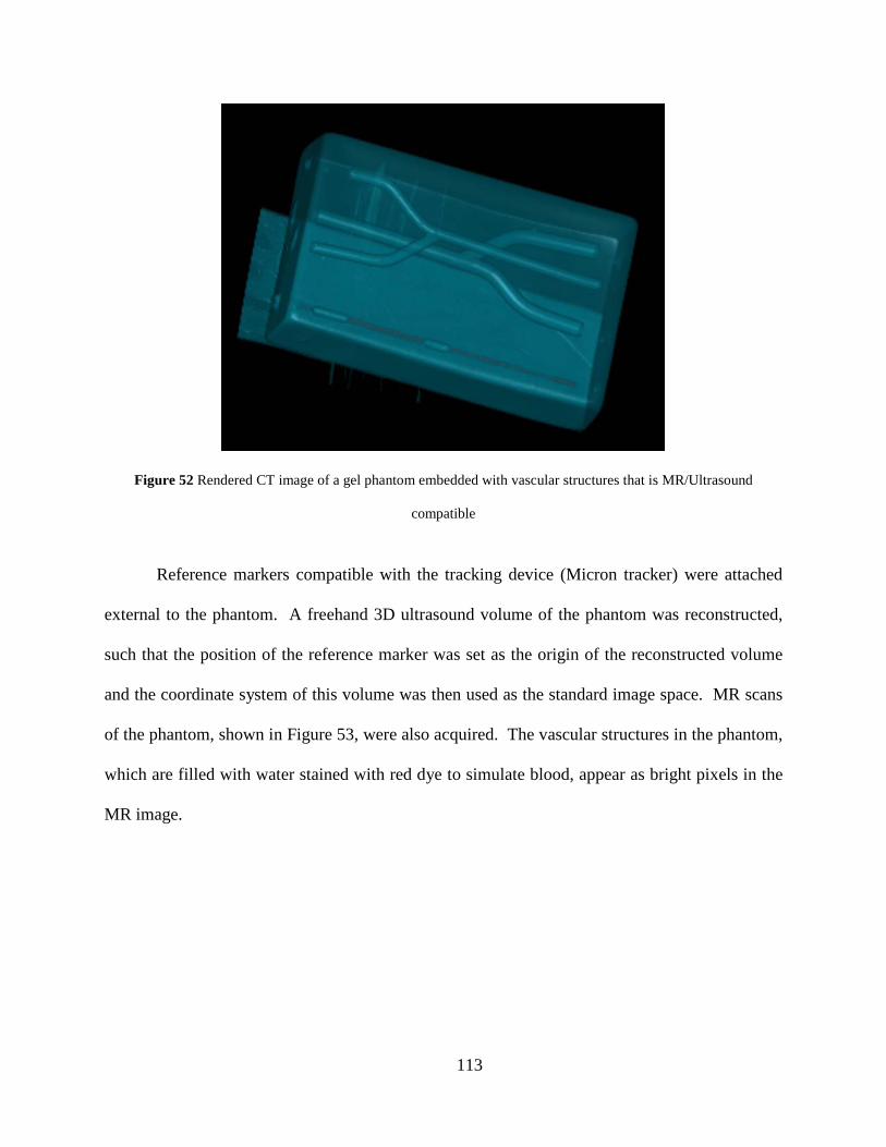
Figure 52 Rendered CT image of a gel phantom embedded with vascular structures that is MR/Ultrasound
compatible
Reference markers compatible with the tracking device (Micron tracker) were attached
external to the phantom. A freehand 3D ultrasound volume of the phantom was reconstructed,
such that the position of the reference marker was set as the origin of the reconstructed volume
and the coordinate system of this volume was then used as the standard image space. MR scans
of the phantom, shown in Figure 53, were also acquired. The vascular structures in the phantom,
which are filled with water stained with red dye to simulate blood, appear as bright pixels in the
MR image.
113

Figure 53 Three orthogonal views of an MR image of the phantom shown in Figure 52
The MR image was registered to the reconstructed ultrasound volume using the landmark
registration method described in section 6.1.1.2. A set of four landmarks were manually
identified in both the MRI and reconstructed ultrasound volume. Figure 54 shows a cross-
sectional view of the reconstructed ultrasound volume overlaid on the registered MR image. We
can see that there is good correspondence in the region of the vessel. The overlay of the
ultrasound image occupies a small area compared to the MRI, because the MR image captures
the full dimensions of the phantom, whereas the ultrasound represents only a small portion of the
phantom.
114

Figure 54 Cross-sectional view of the reconstructed ultrasound volume overlaid on the registered MR image
Finally, we combine the real-time registration into a multi-window system (see Figure
55). By tracking the location and orientation of the ultrasound probe relative to the markers,
correspondence between the current scan and the standard image space are computed. Using this
correspondence, based on the current position and orientation of the probe, image slices from the
reconstructed ultrasound volume and corresponding slices from the MR volume are displayed
concurrently along with the current frame extracted from the ultrasound scanner.
115
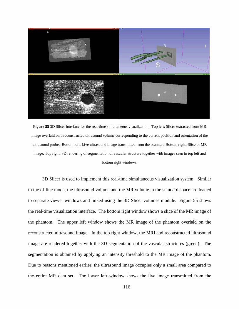
Figure 55 3D Slicer interface for the real-time simultaneous visualization. Top left: Slices extracted from MR
image overlaid on a reconstructed ultrasound volume corresponding to the current position and orientation of the
ultrasound probe. Bottom left: Live ultrasound image transmitted from the scanner. Bottom right: Slice of MR
image. Top right: 3D rendering of segmentation of vascular structure together with images seen in top left and
bottom right windows.
3D Slicer is used to implement this real-time simultaneous visualization system. Similar
to the offline mode, the ultrasound volume and the MR volume in the standard space are loaded
to separate viewer windows and linked using the 3D Slicer volumes module. Figure 55 shows
the real-time visualization interface. The bottom right window shows a slice of the MR image of
the phantom. The upper left window shows the MR image of the phantom overlaid on the
reconstructed ultrasound image. In the top right window, the MRI and reconstructed ultrasound
image are rendered together with the 3D segmentation of the vascular structures (green). The
segmentation is obtained by applying an intensity threshold to the MR image of the phantom.
Due to reasons mentioned earlier, the ultrasound image occupies only a small area compared to
the entire MR data set. The lower left window shows the live image transmitted from the
116
ultrasound scanner. The position and orientation of the probe generated by Micron Tracker is
also transmitted to the interface. OpenIGTLink, which is a set of digital messaging formats and
protocols used for data exchange on a local area network (LAN) for a wide variety of image-
guided therapy (IGT) applications (Tokuda et al., 2009), is used to transmit the live ultrasound
image and the tracking data from their respective sources to the 3D Slicer interface. The
tracking data is used to extract arbitrary slices from the loaded volumes using the reformat
widget in 3D Slicer. The images seen in red, yellow, and 3D viewers in Figure 55 are slices
extracted from the MR and reconstructed ultrasound volumes corresponding to the current
position and orientation of the probe. As seen in the figure, there is good correspondence
between the live image and the slices extracted from previous acquisitions.
117

8.0 DISCUSSION AND FUTURE WORK
The proposed ultrasound imaging system - with the ability to reconstruct 3D volumes from
freehand 2D images and visualize image slices concurrently from different acquisition that
correspond to the same anatomical region - will provide the ability to track changes in
anatomical structures in hand-transplant patients and to monitor nerve regeneration in patients
undergoing regenerative, repair or transplant strategies. The image analysis methods, including
variance descent graphs, the graph based segmentation method that generates communities, and
the hybrid atlas based registration method, will provide a system to study the function and
geometry of various anatomical structures in MR and ultrasound images in a reliable, accurate
and efficient manner.
The freehand 3D reconstruction system described in section 4.0 has advantages over
other 3D ultrasound imaging solutions. Unlike the wobblers and matrix array scanners that can
produce volumes of only a relatively small region of anatomy at a given time, the extent of
anatomy that can be acquired using the freehand system is limited only by the memory capacity
and speed of the computer running the reconstruction algorithm. In addition, operators have
greater control over the reconstruction parameters such as image size, spacing, and the choice of
compounding and bin-fillings methods. The modular nature of the freehand 3D reconstruction
system allows upgrading of individual components with more advanced counterparts without
necessitating major alterations to the rest of the system. For example, it is very straightforward
118
to replace the micron tracker with an advanced version when it becomes available, or to forgo
the optical tracking system completely for a magnetic tracking system. In addition, the same
tracking device can be reused with any conventional 2D probe, with only the recalculation of the
spatial calibration required. Furthermore, the original, raw 2D images from the scanner are
saved and can be made available at a later time. Consequently, advances in reconstruction
techniques can be applied to the images acquired in the past, resulting in better reconstructed
volumes, which can greatly benefit longitudinal studies. Lastly, the tracking system permits
real–time visualization applications such as the one presented in section 7.3.
There are a few drawbacks associated with the freehand 3D reconstruction system.
Although external tracking systems work well in a controlled environment, optical tracking
demands continuous line of sight and magnetic tracking is unpredictable near ferromagnetic
materials. An external tracking system restricts the portability of the US scanner, one of
ultrasound’s great advantages in the hospital. The location of the patient and the particular
anatomical target being scanned must be independently determined. Moreover, a large hole in
the reconstructed image data, too big for the hole-filling methods to interpolate over, may be
created when a significant number of 2D slices are missing at a particular location in 3D space.
In section 6.0 we have presented and validated a framework that enforces local
constraints in any intensity based registration method. In previously reported works
(Papademetris, Jackowski, Schultz, Staib, & Duncan, 2004; W. Peng, Tong, Qian, & Dong,
2006), landmark points are combined with intensity information by considering them as
additional constraints in an optimization problem that are solved by Lagrangian multipliers and
Newton’s method. The advantage of our approach is the versatility in the choice of intensity
based registration. Since landmarks, which are features external to the image, are synthesized as
119

an intrinsic part of the image, any intensity based registration method can be applied on the
resulting fixed and moving images with the assurance that the landmarks will maintain
correspondence. Contrary to the view of losing information by altering the raw image intensity
at landmark locations, we believe the change in intensity at locations with known
correspondence simply provide enhanced image features compatible with intensity based
registration methods. A weakness of the method is that the landmark registration methodology,
which uses anatomical landmarks placed manually by the user to register reconstructed volumes
to standard image space, may be erroneous due to inaccurate positioning of the landmarks, either
because of user error or ambiguity in the reconstructed image data at the landmark locations.
The variance descent graphs method, presented in section 5.3, has some similarities to
other graph-based methods for image segmentation, which generally treat the entire image as a
graph, with each pixel as a node connected to its neighbors by edges. Felzenszwalb and
Huttenlocher’s graph-based segmentation (Felzenszwalb & Huttenlocher, 2004) begins with each
pixel in its own sub-graph, and then joins sub-graphs if the edges between them have a low
enough weight (i.e. the pixels they connect are similar). Edges are examined in order of weight,
so that “easy” connections are made first, leaving the more ambiguous decisions for later in the
algorithm. Our method may also be considered a form of the so-called superpixel (Ren & Malik,
2003), in which over-segmentation based on local similarities preserves most of the structure
while reducing the dimensionality of the overall image (and reducing noise). The contribution of
our work, we believe, is to provide a simple and rapid method to reduce the noise while
preserving meaningful structure in n-dimensional images. The initial step requires only a single
parameter: the radius of the spheres used to compute mean and variance of pixel intensity. VDGs
have been employed in this dissertation to reduce noise in ultrasound images. The method
120

reduces the dimensionality of the images, thus enabling efficient implementation of subsequent
graph based segmentation.
Representation of fascicular anatomy in a regenerating nerve may be complicated by
myelin debris, neuronal edema or axonal disruption. The ultrasound images of the nerve can be
especially noisy, and expert interpretation is required to separate the signals, which include target
anatomy and relevant contextual information, from noise to identify the structures of interest.
We have developed an algorithm (section 5.4) that inherently detects expected shapes - circular
regions - by making use of statistical data computed in robust neighborhoods of an image. Our
method favors circular structures by analyzing local image features in neighborhoods that are
circular (the spheres of influence), and the nature of the voting system guides the assignment of
edge weights such that edges within a potential circular structure receive higher weights than
between such structures. Hence, incomplete boundaries in basically circular structures do not
derail the algorithm and the radius of the S𝑟𝑟(𝐱𝐱) is determined appropriately. The voting system
also ensures that decisions are not induced based on pairwise measures (between individual
pixels, patches, or fragments) but rather by consolidating data in relevant local neighborhoods,
thereby effecting meaningful results even in the presence of high noise. The edge weights
consist of a vector of features instead of a scalar value. Additional image attributes such as color
and texture, and any other derived characteristics, can be included in the feature vector, thus
making the algorithm more robust. Results presented for both 2D and 3D datasets confirm that
the clustering algorithms employed are suitable to form fragments and perform the subsequent
segmentation. The modular design facilitates testing other clustering algorithms in our future
work that includes vascular images acquired using HRUS.
121
The image analysis system comprises distinct methods connected to each other in a
pipeline. The output of the first method is passed as the input to the second. It is possible for
one of the methods to induce errors into the system or even fail completely when applied to a
different application, propagating the errors along the pipeline. However, the methods are
modular in nature, such that each module in the overall system is independent and
interchangeable. During implementation, if any one of the modules does not produce
satisfactory results, it can easily be replaced with a different method. For example, when image
noise is not prominent, the VDGs can be replaced with any other data dimensionality reduction
technique. The affinity propagation and dominant sets clustering algorithms can also be replaced
with other graph based clustering techniques.
8.1 FUTURE DIRECTIONS
In this section, avenues of future work are discussed. It is possible to overcome the issues
related to large holes in the reconstructed volume by extracting data from previous volumes. The
correspondence between the current location of the US probe and the standard image space can
be computed by methods discussed in the real-time playback scenario (section 7.3). Since the
previous and prior volumes are registered to the standard image space, hole-filling methods may
be extended to utilize data from other images at locations corresponding to the missing US data.
The identification of anatomical landmarks, which are critical for registering volumes to the
standard image space, could also be facilitated using the same approach.
The simultaneous visualization system should be applied next to a human arm. During
each scan, the subject’s arm will be held rigidly by a brace. The brace will be MRI/CT
122

compatible and attached with commercially available multi-modality markers that are visible in
MRI/CT and to the tracking system ("Multi-Modality Markers,"). The brace will be placed at a
precise location on the arm ensuring that the markers are at a specific location relative to the arm
consistently from one scan to the next.
To account for physical deformation between scans, or within scans due to the ultrasound
probe, the hybrid registration can be modeled with the Finite Element Method (FEM)
(Hagemann, Rohr, Stiehl, Spetzger, & Gilsbach, 1999; Kyriacou, Davatzikos, Zinreich, & Bryan,
1999). In this method, the image is modeled as a physical body, on which external forces that
govern deformations in the body are applied. Physical characteristics such as elasticity and
density associated with the body determine the degree of deformation of the physical body. The
external forces can correspond to image attributes (intensity), or they can be user defined
landmarks. With this approach, landmarks can be coupled with intensity information within the
same optimization criterion.
8.1.1 ProbeSight
The aforementioned problems related to external tracking systems can be addressed with a
technique we are developing in our laboratory, called ProbeSight. It is a system for guiding
ultrasound probes and other clinical tools with respect to the exterior of the patient, using one or
more video camera(s) mounted directly on the probe or tool. Real-time video images of the
patient’s exterior are matched against a prior high-resolution surface map acquired with a high
resolution multiple-camera imaging device used in plastic surgery (J. Wang et al., 2014). This
surface map is rendered from multiple viewpoints in real-time to find the viewpoint that best
matches the probe-mounted camera image, thus establishing the camera’s pose relative to the
123

anatomy. For ultrasound, this will permit freehand 3D reconstruction, as well as simultaneous
visualization of real-time ultrasound and previous acquisitions from the same anatomical
location, all without using external tracking devices. Thus ProbeSight will permit the ultrasound
methods described in this dissertation to be used in a more practical manner in the hospital
setting.
124
BIBLIOGRAPHY
3D Imaging Using 2D CMUT Arrays with Integrated Electronics.). from http://www-kyg.stanford.edu/khuriyakub/opencms/en/research/ultrasonic/3D_Imaging/index.html
Aylward, Stephen R, & Bullitt, Elizabeth. (2002). Initialization, noise, singularities, and scale in height ridge traversal for tubular object centerline extraction. Medical Imaging, IEEE Transactions on, 21(2), 61-75.
Balafar, M. A., Ramli, A. R., Saripan, M. I., & Mashohor, S. (2010). Review of brain MRI image segmentation methods. Artificial Intelligence Review, 33(3), 261-274. doi: 10.1007/s10462-010-9155-0
Barker, J. H., Francois, C. G., Frank, J. M., & Maldonado, C. (2002). Composite tissue allotransplantation. Transplantation, 73(5), 832-835.
Barrett, William A, & Mortensen, Eric N. (1997). Interactive live-wire boundary extraction. Medical Image Analysis, 1(4), 331-341.
Blue Phantom Inc. Boykov, Yuri, & Kolmogorov, Vladimir. (2004). An experimental comparison of min-cut/max-
flow algorithms for energy minimization in vision. Pattern Analysis and Machine Intelligence, IEEE Transactions on, 26(9), 1124-1137.
Boykov, Yuri Y, & Jolly, M-P. (2001). Interactive graph cuts for optimal boundary & region segmentation of objects in ND images. Paper presented at the Computer Vision, 2001. ICCV 2001. Proceedings. Eighth IEEE International Conference on.
Brown, Lisa Gottesfeld. (1992). A survey of image registration techniques. ACM computing surveys (CSUR), 24(4), 325-376.
Burnett, M. G., & Zager, E. L. (2004). Pathophysiology of peripheral nerve injury: a brief review. Neurosurg Focus, 16(5), E1.
Canny, John. (1986). A computational approach to edge detection. Pattern Analysis and Machine Intelligence, IEEE Transactions on(6), 679-698.
Carmichael, Owen T, Aizenstein, Howard A, Davis, Simon W, Becker, James T, Thompson, Paul M, Meltzer, Carolyn Cidis, & Liu, Yanxi. (2005). Atlas-based hippocampus segmentation in Alzheimer's disease and mild cognitive impairment. Neuroimage, 27(4), 979-990.
Chen, Chaur-Chin, & Huang, Chung-Ling. (1993). Markov random fields for texture classification. Pattern Recognition Letters, 14(11), 907-914.
125

Chen, Mei, Kanade, Takeo, Pomerleau, Dean, & Schneider, Jeff. (1999). 3-D deformable registration of medical images using a statistical atlas. Paper presented at the Medical Image Computing and Computer-Assisted Intervention–MICCAI’99.
Chen, Thomas Kuiran, Thurston, Adrian D, Ellis, Randy E, & Abolmaesumi, Purang. (2009). A real-time freehand ultrasound calibration system with automatic accuracy feedback and control. Ultrasound in medicine & biology, 35(1), 79-93.
Cox, Ingemar J, Rao, Satish B, & Zhong, Yu. (1996). “Ratio regions”: A technique for image segmentation. Paper presented at the Pattern Recognition, 1996., Proceedings of the 13th International Conference on.
Cremers, Daniel. (2006). Dynamical statistical shape priors for level set-based tracking. Pattern Analysis and Machine Intelligence, IEEE Transactions on, 28(8), 1262-1273.
Das, Piali, Veksler, Olga, Zavadsky, Vyacheslav, & Boykov, Yuri. (2009). Semiautomatic segmentation with compact shape prior. Image and Vision Computing, 27(1), 206-219.
Dewi, D.E.O., Wilkinson, M.H.F., Mengko, T.L.R., Purnama, I.K.E., van Ooijen, P.M.A., Veldhuizen, A.G., . . . Verkerke, G.J. (2009). 3D Ultrasound Reconstruction of Spinal Images using an Improved Olympic Hole-Filling Method. Paper presented at the International Conference on Instrumentation, Communication, Information Technolohgy, and Biomedical Engineering (ICICI-BME).
Egghe, Leo. (2009). New relations between similarity measures for vectors based on vector norms. Journal of the American Society for Information Science and Technology, 60(2), 232-239. doi: 10.1002/asi.20949
Estépar, Raúl San José, Martín-Fernández, Marcos, Alberola-López, Carlos, Ellsmere, James, Kikinis, Ron, & Westin, Carl-Fredrik. (2003). Freehand ultrasound reconstruction based on roi prior modeling and normalized convolution Medical Image Computing and Computer-Assisted Intervention-MICCAI 2003 (pp. 382-390): Springer.
Falcão, Alexandre X, Udupa, Jayaram K, & Miyazawa, Flavio Keidi. (2000). An ultra-fast user-steered image segmentation paradigm: live wire on the fly. Medical Imaging, IEEE Transactions on, 19(1), 55-62.
Fedorov, Andriy, Beichel, Reinhard, Kalpathy-Cramer, Jayashree, Finet, Julien, Fillion-Robin, Jean-Christophe, Pujol, Sonia, . . . Sonka, Milan. (2012). 3D Slicer as an image computing platform for the Quantitative Imaging Network. Magnetic Resonance Imaging.
Felzenszwalb, Pedro F, & Huttenlocher, Daniel P. (2004). Efficient graph-based image segmentation. International Journal of Computer Vision, 59(2), 167-181.
Fischl, Bruce, Salat, David H, Busa, Evelina, Albert, Marilyn, Dieterich, Megan, Haselgrove, Christian, . . . Klaveness, Shuna. (2002). Whole brain segmentation: automated labeling of neuroanatomical structures in the human brain. Neuron, 33(3), 341-355.
Fornefett, M., Rohr, K., & Stiehl, H. S. (2001). Radial basis functions with compact support for elastic registration of medical images. Image and Vision Computing, 19(1-2), 87-96. doi: Doi 10.1016/S0262-8856(00)00057-3
126
Freedman, D., & Tao, Zhang. (2005). Interactive Graph Cut Based Segmentation with Shape Priors. 1, 755-762. doi: 10.1109/cvpr.2005.191
Frey, Brendan J, & Dueck, Delbert. (2007). Clustering by passing messages between data points. science, 315(5814), 972-976.
Friston, Karl, Ashburner, John, Frith, Christopher D, Poline, J‐B, Heather, John D, & Frackowiak, Richard SJ. (1995). Spatial registration and normalization of images. Human brain mapping, 3(3), 165-189.
Goshtasby, Ardeshir, & Le Moign, J. (2012). Image registration: Springer. Grady, Leo. (2005). Multilabel random walker image segmentation using prior models. Paper
presented at the Computer Vision and Pattern Recognition, 2005. CVPR 2005. IEEE Computer Society Conference on.
Grady, Leo. (2006). Random walks for image segmentation. Pattern Analysis and Machine Intelligence, IEEE Transactions on, 28(11), 1768-1783.
Hagemann, Alexander, Rohr, Karl, Stiehl, H. Siegfried, Spetzger, Uwe, & Gilsbach, Joachim M. (1999). Biomechanical modeling of the human head for physically based, nonrigid image registration. Medical Imaging, IEEE Transactions on, 18(10), 875-884.
Hand Registry. Retrieved from http://www.handregistry.com Hough, Paul VC. (1962). Method and means for recognizing complex patterns: Google Patents. Hsu, Po-Wei, Prager, Richard W, Gee, Andrew H, & Treece, Graham M. (2008). Real-time
freehand 3D ultrasound calibration. Ultrasound in medicine & biology, 34(2), 239-251. http://www.slicer.org.). Ibanez, Luis, Schroeder, William, Ng, Lydia, & Cates, Josh. (2003). The ITK software guide. Jain, Anil K. (1989). Fundamentals of digital image processing: Prentice-Hall, Inc. Jenkinson, Mark, Bannister, Peter, Brady, Michael, & Smith, Stephen. (2002). Improved
optimization for the robust and accurate linear registration and motion correction of brain images. Neuroimage, 17(2), 825-841.
Johnson, Hans, & Zhao, Yongqiang. (2009). Brainsdemonwarp: An applicaton to perform demons registration. The Insight Journal.
Kass, Michael, Witkin, Andrew, & Terzopoulos, Demetri. (1988). Snakes: Active contour models. International journal of computer vision, 1(4), 321-331.
Kaufman, CL, Ouseph, R, Blair, B, Kutz, JE, Tsai, TM, Scheker, LR, . . . Banegas, R. (2012). Graft Vasculopathy in Clinical Hand Transplantation. American Journal of Transplantation.
Keith, J, Fletcher, D, Kim, K, Brandacher, G, Shores, J, Lee, WPA, . . . Gorantla, VS. (2012). High Resolution Ultrasound for Noninvasive Monitoring of Graft Vasculopathy after Human Upper Extremity Transplantation: 2310. Transplantation, 94(10S), 366.
Kesley, J., Praemer, A., Nelson, L., Felberg, A., & Rice, D. (1997) Upper extremity disorders: frequency, impact, and cost (pp. 26,42): Churchill Livingstone.
127
Kremkau, FW, & Taylor, KJ. (1986). Artifacts in ultrasound imaging. Journal of ultrasound in medicine, 5(4), 227-237.
Kyriacou, Stelios K, Davatzikos, Christos, Zinreich, S James, & Bryan, R Nick. (1999). Nonlinear elastic registration of brain images with tumor pathology using a biomechanical model [MRI]. Medical Imaging, IEEE Transactions on, 18(7), 580-592.
Laakso, M. P., Soininen, H., Partanen, K., Helkala, E. L., Hartikainen, P., Vainio, P., . . . Riekkinen, P. J., Sr. (1995). Volumes of hippocampus, amygdala and frontal lobes in the MRI-based diagnosis of early Alzheimer's disease: correlation with memory functions. J Neural Transm Park Dis Dement Sect, 9(1), 73-86.
Lasso, A, Heffter, T, Rankin, A, Pinter, C, Ungi, T, & Fichtinger, G. (2014). PLUS: open-source toolkit for ultrasound-guided intervention systems.
Liang, Zhi-Pei, & Lauterbur, Paul C. (2000). Principles of magnetic resonance imaging: SPIE Optical Engineering Press.
Liao, Ping-Sung, Chen, Tse-Sheng, & Chung, Pau-Choo. (2001). A fast algorithm for multilevel thresholding. J. Inf. Sci. Eng., 17(5), 713-727.
Mallat, Stephane, & Zhong, Sifen. (1992). Characterization of signals from multiscale edges. IEEE Transactions on pattern analysis and machine intelligence, 14(7), 710-732.
Martin, K, & Hoffman, B. (2010). Mastering CMake: A Cross-Platform Build System. Kitware. Inc., Clifton Park, NY, 5.
McInerney, Tim, & Terzopoulos, Demetri. (1996). Deformable models in medical image analysis: a survey. Medical image analysis, 1(2), 91-108.
Micron Tracker.). from http://www.clarontech.com/microntracker.php Modersitzki, Jan. (2004). Numerical Methods for Image Registration (Numerical Mathematics
and Scientific Computation): Oxford university press USA. Morris, OJ, Lee, M de J, & Constantinides, AG. (1986). Graph theory for image analysis: an
approach based on the shortest spanning tree. Communications, Radar and Signal Processing, IEE Proceedings F, 133(2), 146-152.
Noble, J. A., & Boukerroui, D. (2006). Ultrasound image segmentation: a survey. IEEE Trans Med Imaging, 25(8), 987-1010.
Papademetris, Xenophon, Jackowski, Andrea P, Schultz, Robert T, Staib, Lawrence H, & Duncan, James S. (2004). Integrated intensity and point-feature nonrigid registration Medical Image Computing and Computer-Assisted Intervention–MICCAI 2004 (pp. 763-770): Springer.
Patenaude, Brian, Smith, Stephen M, Kennedy, David N, & Jenkinson, Mark. (2011). A Bayesian model of shape and appearance for subcortical brain segmentation. Neuroimage, 56(3), 907-922.
Pavan, Massimiliano, & Pelillo, Marcello. (2003). A new graph-theoretic approach to clustering and segmentation. Paper presented at the Computer Vision and Pattern Recognition, 2003. Proceedings. 2003 IEEE Computer Society Conference on.
128
Peng, Bo, Zhang, Lei, & Zhang, David. (2013). A survey of graph theoretical approaches to image segmentation. Pattern Recognition, 46(3), 1020-1038.
Peng, Wen, Tong, Ruofeng, Qian, Guiping, & Dong, Jinxiang. (2006). A hybrid registration of medical images using intensity information and landmark points. Paper presented at the Signal Processing, 2006 8th International Conference on.
Petrou, Maria, & Petrou, Costas. (2010). Image processing: the fundamentals: John Wiley & Sons.
Pieper, S., Lorensen, B., Schroeder, W., & Kikinis, R. (2006, 6-9 April 2006). The NA-MIC Kit: ITK, VTK, pipelines, grids and 3D slicer as an open platform for the medical image computing community. Paper presented at the Biomedical Imaging: Nano to Macro, 2006. 3rd IEEE International Symposium on.
Pluta, John, Avants, Brian B, Glynn, Simon, Awate, Suyash, Gee, James C, & Detre, John A. (2009). Appearance and incomplete label matching for diffeomorphic template based hippocampus segmentation. Hippocampus, 19(6), 565-571.
Pratt, William K. (1991). Digital image processing: Wiley, New York. Rand, William M. (1971). Objective criteria for the evaluation of clustering methods. Journal of
the American Statistical association, 66(336), 846-850. Ren, & Malik. (2003). Learning a classification model for segmentation. 10-17 vol.11. doi:
10.1109/iccv.2003.1238308 Revanna Shivaprabhu, Vikas. (2010). Automated Method for N-Dimensional Shape Detection
Based On Medial Image Features. University of Pittsburgh. Rohling, R., Gee, A., & Berman, L. (1999). A comparison of freehand three-dimensional
ultrasound reconstruction techniques. Med Image Anal, 3(4), 339-359. Rousseau, F., Hellier, P., & Barillot, C. (2006). A novel temporal calibration method for 3-D
ultrasound. Medical Imaging, IEEE Transactions on, 25(8), 1108-1112. Rousseau, François, Hellier, Pierre, & Barillot, Christian. (2005). Confhusius: A robust and fully
automatic calibration method for 3D freehand ultrasound. Medical image analysis, 9(1), 25-38.
Sharp, GC, Li, R, Wolfgang, J, Chen, G, Peroni, M, Spadea, MF, . . . Kandasamy, N. (2010). PLASTIMATCH—An open source software suite for radiotherapy image processing. Paper presented at the Proceedings of the International Conference on the use of Computers in Radiotherapy (ICCR), Amsterdam, the Netherlands.
Shi, J., & Malik, J. (2000). Normalized cuts and image segmentation. Pattern Analysis and Machine Intelligence, IEEE Transactions on, 22(8), 888-905. doi: 10.1109/34.868688
Siddiqi, Kaleem, & Pizer, Stephen M. (2008). Medial representations: mathematics, algorithms and applications (Vol. 37): Springer.
Sled, John G, Zijdenbos, Alex P, & Evans, Alan C. (1998). A nonparametric method for automatic correction of intensity nonuniformity in MRI data. Medical Imaging, IEEE Transactions on, 17(1), 87-97.
129
Smith, Stephen M. (2002). Fast robust automated brain extraction. Human brain mapping, 17(3), 143-155.
Solberg, O.V., Lindseth, F., Torp, H., Blake, R.E., & Nagelhus, T.A. (2007). Freehand 3D Ultrasound Reconstructionh Algorithm A Review. Ultrasound in medicine & biology, 33(7), 991-1009.
Späth, Helmuth. (2004). Fitting affine and orthogonal transformations between two sets of points. Mathematical Communications, 9(1), 27-34.
Stetten, George D, & Pizer, Stephen M. (1999). Medial-node models to identify and measure objects in real-time 3-D echocardiography. Medical Imaging, IEEE Transactions on, 18(10), 1025-1034.
Stetten, George, Horvath, Samantha, Galeotti, John, Shukla, Gaurav, Wang, Bo, & Chapman, Brian. (2010). Image segmentation using the student's t-test and the divergence of direction on spherical regions. 76233I-76233I. doi: 10.1117/12.844014
Stetten, George, Wong, Cindy, Shivaprabhu, Vikas, Zhang, Ada, Horvath, Samantha, Wang, Jihang, . . . Aizenstein, Howard. (2013). Descending Variance Graphs for Segmenting Neurological Structures.
Thies, William, & Bleiler, Laura. (2013). 2013 Alzheimer's disease facts and figures. Alzheimer's & dementia: the journal of the Alzheimer's Association, 9(2), 208-245.
Thirion, J-P. (1998). Image matching as a diffusion process: an analogy with Maxwell's demons. Medical image analysis, 2(3), 243-260.
Toennies, Klaus D. (2012). Guide to Medical Image Analysis. Tokuda, Junichi, Fischer, Gregory S, Papademetris, Xenophon, Yaniv, Ziv, Ibanez, Luis, Cheng,
Patrick, . . . Golby, Alexandra J. (2009). OpenIGTLink: an open network protocol for image‐guided therapy environment. The International Journal of Medical Robotics and Computer Assisted Surgery, 5(4), 423-434.
Tuffaha, Sami, Quigley, Meghan, Ng, Timothy, Gorantla, Vijay S, Shores, Jaimie T, Pulikkottil, Benson, . . . Lee, WP. (2011). The effect of chondroitinase on nerve regeneration following composite tissue allotransplantation. The Journal of hand surgery, 36(9), 1447-1452.
Vercauteren, Tom, Pennec, Xavier, Perchant, Aymeric, & Ayache, Nicholas. (2007). Non-parametric diffeomorphic image registration with the demons algorithm Medical Image Computing and Computer-Assisted Intervention–MICCAI 2007 (pp. 319-326): Springer.
Wang, Jihang, Shivaprabhu, Vikas, Galeotti, John, Horvath, Samantha, Gorantla, Vijay, & Stetten, George. (2014). Towards Video Guidance for Ultrasound, Using a Prior High-Resolution 3D Surface Map of the External Anatomy Augmented Environments for Computer-Assisted Interventions (pp. 51-59): Springer.
Wang, Song, & Siskind, Jeffrey Mark. (2001). Image segmentation with minimum mean cut. Paper presented at the Computer Vision, 2001. ICCV 2001. Proceedings. Eighth IEEE International Conference on.
130

Wang, Song, & Siskind, Jeffrey Mark. (2003). Image segmentation with ratio cut. Pattern Analysis and Machine Intelligence, IEEE Transactions on, 25(6), 675-690.
Webb, Andrew, & Kagadis, George C. (2003). Introduction to biomedical imaging. Medical Physics, 30(8), 2267-2267.
Wendland, Holger. (1995). Piecewise polynomial, positive definite and compactly supported radial functions of minimal degree. Advances in computational Mathematics, 4(1), 389-396.
Woods, Roger P, Grafton, Scott T, Holmes, Colin J, Cherry, Simon R, & Mazziotta, John C. (1998). Automated image registration: I. General methods and intrasubject, intramodality validation. Journal of computer assisted tomography, 22(1), 139-152.
Wu, Zhenyu, & Leahy, Richard. (1993). An optimal graph theoretic approach to data clustering: Theory and its application to image segmentation. Pattern Analysis and Machine Intelligence, IEEE Transactions on, 15(11), 1101-1113.
Yoo, Terry S. (2004). Insight into images: principles and practice for segmentation, registration, and image analysis: AK Peters Ltd.
131