trends and determinants of research driven total...

Trends and Determinants of Research Driven Total Factor Productivity in Indian Wheat By Sendhil R1, Ramasundaram P2, Anbukkani P3, Randhir Singh1 and Indu Sharma1

1ICAR-Indian Institute of Wheat and Barley Research, Karnal, Haryana, India

2ICAR-National Agricultural Education Project, Krishi Anusandhan Bhavan II, Pusa, New Delhi, India

3ICAR-Indian Agricultural Research Institute, Pusa, New Delhi, India

Productivity, technology and efficiency drive agricultural growth through research.

The total factor productivity (TFP) being increase in rate of growth of output over the

rate of growth of inputs, its decline is a major concern and policy priority in the

context of sustainable food production. This paper examines the wheat TFP in India

during 2001-02 to 2010-11 across regions. The TFP determinants were discussed in

terms of technological progress and technical efficiency. Inputs usage barring human

labor and animal power, was intensive and registered positive growth. The mean TFP

declined by 1 per cent. The slowdown is attributed to decline in the technological

progress by 1.1 per cent despite a marginal increase in the efficiency by 0.1 per cent.

The capital intensive new sciences need to be harnessed for breaking yield barriers.

Higher allocation of funds to research and extension is needed for technological

progress and efficiency gains.

1

1. Introduction

Ensuring food security is an utmost concern and a policy priority. Hence, formulating strategies

becomes the focus of several countries and major agenda in policy forums. Research thrust is on

increasing the crop productivity in tandem with minimal resources (inputs) focusing on breaking

the yield barrier with new genotypes and management practices given the investment.

Wheat (Triticum spp.) is the second most important staple food crop of India grown in 30

million hectares across six agro-climatic zones. It is one of the cheapest and nutritious cereals

accounting for about 20 per cent of total protein supply and 19 per cent of total calorie intake. The

production growth rate estimated at 6.82 per cent per annum during the 1960s has drastically

declined to 1.90 per cent (Sendhil et al., 2012). Historical data reveal that intensive use of inputs

post-Green Revolution (henceforth GR) puts a heavy strain on the production. Hence, intense

research on productivity growth in wheat has become a matter of serious concern in the recent past.

The GR introduced in the mid-1960s through high yielding semi-dwarf genotypes (or varieties)

responsive to chemical fertilizers coupled with research, training and extension, irrigation and

infrastructures helped immensely to increase the productivity (Chand et al., 2011). However, the

incremental yield and social benefit due to adoption of an improved technology could not spread

evenly owing to diverse agro-climatic conditions and varying natural resource endowments

(Hayami and Kikuchi, 1999). The stagnation in production and productivity during 1980s has

become a matter of concern for the researchers. Productivity growth measured by total factor

productivity (TFP) declined after the GR era attributed to technology fatigue or policy failure

(Narayanamoorthy, 2007). But, there is a lack of empirical evidence to show whether the declining

productivity growth has revived in the recent past. This context provides the rationale for the

present study.

Globally, the yield of wheat has to be increased by 60 per cent within 2050 to match the

projected food demand (Ray et al., 2013). In India, the average yield has to be raised to 4.5 tonnes

per hectare by 2050 to produce 140 million tonnes from the current national average of 3.1 tonnes

per hectare. Analyzing the productivity growth is much more important from the view point of

concerted efforts made by the Government of India, through various developmental programmes

like National Food Security Mission (NFSM) have been launched for accelerating growth in the

agricultural sector. It is imperative to analyze the periodical trends in TFP and discuss its

determinants for policy formulations and programme planning. The present study aims to estimate

the recent spatial and temporal trends in the TFP growth along with the growth in output and input

variables. Besides, the determinants of TFP in terms of technological progress and technical

efficiency were also discussed for drawing policies.

2

2. TFP – Conceptual Background and Research Progress in Wheat

Technically, productivity is defined as the ratio of output to input. Estimation of partial productivity

with respect to a specific input viz., land, labor and capital is of limited use since agricultural

production relation involves multiple inputs and outputs that are joint and inseparable. The TFP

takes care of this and relates aggregate output index to aggregate input index (Kannan, 2011). It is

an appropriate technique for examining and understanding the growth in crop productivity and

separates the effect of inputs and other factors like technology, infrastructure, and farmers’

knowledge on productivity growth (Chand et al, 2011). It is the extension of the partial factor

productivity analysis and non-parametric in nature (Grosskopf, 1993) and can be measured by

different approaches (Christensen, 1975) like arithmetic computation, geometric measurement and

formulation of indices developed by Tornqvist-Theil in 1976 called as Divisia index or Tornqvist-

Divisia index or Tornqvist-Theil index (Diewert, 1976).

A number of research studies have been carried out on the measurement of productivity

pertaining to agriculture sector and specific crops. Most of them estimated the effect of

technological change on agriculture as a whole or total crop sector. Murgai (1999 and 2005) using

Tornqvist-Theil index estimated the TFP growth in Punjab during 1960-1993 as 1.9 per cent, lowest

even during the GR years, when farmers moved from traditional to modern varieties of wheat and

the sector experienced spectacular shifts in production as indicated by high growth rates. The study

attributed most yield improvements to rapid factor accumulation, particularly that of fertilizers and

capital. Kumar and Mittal (2006) estimated TFP growth across different states and found that the

TFP is still growing in the two green revolution states viz., Haryana and Punjab. Chand et al (2011)

estimated the TFP for different crops during 1986-2005 using Divisia-Tornqvist index. They found

that the TFP growth was highest for wheat. Bhushan (2005) used data envelopment analysis (DEA)

based Malmquist TFP index for major wheat producing states and found that TFP growth rate to be

highest in Punjab and Haryana. As compared to 1980s, mean growth of TFP is found to be higher in

1990s and the primary source of TFP growth is identified as technological progress and not

efficiency improvements. Yet, due to non-availability of proper input consumption data across

crops, the estimated TFP growth was expected to be more or less from the actual (Chand et al,

2011). Despite this limitation, Sidhu and Byerlee (1992), Kumar and Mruthyunjaya (1992), Kumar

and Rosegrant (1994), Kumar (2001), Baset et al. (2009), Chand et al. (2011), Kannan (2011) and

Chaudhary (2012) estimated the TFP for individual crops. Although voluminous literature is

available on TFP estimation, no study on spatial and temporal trends in TFP growth as well as its

determinants is available for wheat that extends to recent years. The present study is an attempt to

fill the existing research and knowledge gap for researchers and policy makers.

3

3. Data and Methodology

Secondary data on output produced and inputs used from 2001-02 to 2010-11 have been sourced

from the Cost of Cultivation reports published by the Directorate of Economics and Statistics,

Government of India. The input and output variables used for this study has been considered

following Bhushan (2005). However, for some inputs like machine power and irrigation charges,

only value at current prices (Indian National Rupee-INR) is available owing to computation

problems. These inputs are deflated using consumer price indices with the base year as 2001-02.

TFP indices for 1980s and 1990s were sourced from Bhushan (2005) for comparing with the recent

decade. Supporting data on released genotypes were collected from the published documents of the

ICAR-Indian Institute of Wheat and Barley Research.

3.1. Trend Analysis

Apart from the conventional tools like tabular analysis and graphs, compound annual growth rates

(CAGR) were computed using ordinary least squares (Gujarati, 2003) for identifying the trends.

3.2. Malmquist TFP Index

The TFP has been estimated using the Malmquist index of productivity (MIP) introduced by Caves

et al. (1982). It is an output oriented index which measures the maximum level of output that can be

produced using a given level of inputs and technology. This section briefly describes the theory

behind the estimation of Malmquist TFP index. A production function involving multiple outputs

and inputs, denoted by the technology set S can be defined as follows:

S={(x, y): x can produce y} (1)

where,

x represent a N x 1 input vector of non-negative real numbers and y denote a non-negative M x 1

output vector. This set consists of all input-output vectors (x, y) such that a bundle of ‘x’ can

produce ‘y’. Farrell (1957) posited the piece-wise linear convex hull approach to estimate

production frontier, however, its wide application increased only after Charnes et al.(1978) coining

the term Data Envelopment Analysis (DEA). DEA is a non-parametric method that involves the

use of linear programming to construct a piece-wise surface (or production frontier) over the data

points enveloping all given data points (hence the name DEA) such that all the observed data points

lie on or below the frontier. Efficiency measures are calculated in relation to the production frontier.

DEA, typically uses the ‘distance functions’ to describe the multi-input and multi-output production

technology without explicitly stating any objective function like cost-minimization or profit-

maximization.

4

Theoretically, distance functions can be either output- or input-oriented. An output distance

function considers the maximum expansion of the output vector in proportion to the bundle of input

vectors. Alternatively, it measures the distance of a farm from its production frontier. The output

distance function at time t as defined by Fare et al. (1994) is given as:

1

0 })),(:(sup{})/,(:inf{),( ttttttttt SyxSyxyxD (2)

Distance function are the inverse of the maximum proportional increase in the output vector yt,

given the set of inputs xt and production technology St. The computation is equivalent to the

Farrell’s (1957) measure of technical efficiency but in reciprocal term. The superscript refers to the

base year in which the production frontier was used as reference technology. The computation can

be illustrated diagrammatically as in Figure 1.

The production possibility sets are depicted for periods, t and t+1 (Figure 1) for two

production units (a wheat farm in our case), A and B. In the figure, farm B lies on the production

frontier in both the time periods indicating it is cent per cent efficient technically. However, for firm

A which lie inside the frontier, the distance from the production point to the frontier in time period

t, that is, Dto(xt,yt) is given by OAt/ OBt. This ratio is less than one as the firm is technically

inefficient. In the case of farm B, the distance from its production point to the frontier shall be equal

to one as it lies on the frontier. Farm A’s distance function in time period t+1, Dt+1o(xt+1,yt+1), is

represented as OAt+1/ OBt+1. Comparing the two distance functions will reveal the performance of

farm A on efficiency front. If the farm A has become more efficient in time period t+1 than it was

in time period t, then its production point in t+1 would be closer to the same period frontier than in

the preceding period. In other words, the distance computed from Dt+1o(xt+1, yt+1) would be greater

than Dto(xt,yt). The above distances are calculated from same period’s production frontier.

However, the distances can also be computed using some other period’s production frontier /

technology as well. For instance, in the case of farm A, distance of its production point in time

period t can be calculated with respect to frontier of time period t+1. This distance, Dt+1o(xt,yt) is

given by OAt/ OBt+1. Similarly, the distance of farm A’s production point in time period t+1 can be

computed using time period t’s frontier as reference technology. This distance, Dto(xt+1,yt+1), is

given by OAt+1/ OBt. A comparison of these mixed-period distance functions shall reveal whether

the technical change has taken place or not. If what is produced in time period t+1 could not have

been produced in time period t, then the distance Dto(xt+1,yt+1) would be greater than one. Similarly,

if the distance computed of period t’s production point from period t+1’s frontier exceeds that from

period t’s frontier, that is Dt+1o(xt,yt) > Dt

o(xt,yt), then it implies an outward shift of production

frontier in time period t+1.

5

Caves et al. (1982) defined the TFP index using Malmquist input and output distance

functions, and thus the resulting index at period t is popularly known as the Malmquist TFP index.

M t = ),(

),( 11

ttt

o

ttt

o

yxD

yxD

(3)

Caves et al. (1982) expressed the productivity index as the ratio of two output distance functions

taking technology at time t as the reference. Instead of using period t’s technology as the reference,

it is possible to construct output distance functions based on period (t+1)’s technology and thus

another Malmquist productivity index can be laid down as:

M t+1 = ),(

),(1

111

ttt

o

ttt

o

yxD

yxD

(4)

Fare et al. (1994) attempted to remove the arbitrariness in the choice of benchmark by specifying

the Malmquist productivity change index as the geometric mean of the two-period indices, and

given as:

Mo (xt+1, yt+1, x t, y t) =

2

1

1

11111

),(

),(

),(

),(

ttt

o

ttt

o

ttt

o

ttt

o

yxD

yxD

yxD

yxD (5)

Using simple arithmetic, the equation (5) can be written as the product of two distinct components

viz., technical change (technological progress) and efficiency change (Fare et al., 1994).

Mo (xt+1, yt+1, x t, y t) =

2

1

1111

11111

),(

),(

),(

),(

),(

),(

ttt

o

ttt

o

ttt

o

ttt

o

ttt

o

ttt

o

yxD

yxD

yxD

yxD

yxD

yxD (6)

where,

Efficiency change = ),(

),( 111

ttt

o

ttt

o

yxD

yxD

(7)

Technological progress change =

),(

),(

),(

),(1111

11

ttt

o

ttt

o

ttt

o

ttt

o

yxD

yxD

yxD

yxD (8)

Hence the Malmquist productivity index is simply the product of the change in relative efficiency

that occurred between periods t and t+1, and the change in technology that occurred between

periods t and t+1. Several studies viz., Trueblood (1996), Arnade (1998), Fulginiti and Perrin

(1998), Forstner and Isaksson (2002), Nin et al (2003), Coelli et al (2003), Coelli and Rao (2003),

Rahman (2004), Alene (2009) and Chaudhary (2012) used the Malmquist index based approach.

Estimation of MIP through linear programming has four relative advantages (Fare et al., 1994): (i)

computation requires only the quantity of inputs and output; (ii) does not assume any production

function; (iii) no a priori assumption on optimization of the selected farms; and, (iv) decomposes

the TFP into technological progress and efficiency change. The analysis has been carried out by

using DEAP 2.1 software developed by Coelli (1996).

6

4. Results and Discussion

4.1. Growth in Wheat Output and Inputs

This study looks into the changes in productivity, efficiency, and technology in wheat production

for the period 2001-02 to 2010-11. In the previous section, MIP growth was defined relative to a

reference technology for the period of the study. Using this information, two primary issues are

addressed in our computation of MIP growth. The first is the measurement of productivity change

over the period. The second is to decompose changes in productivity into what are generally

referred to as a ‘catching-up’ effect (efficiency change) and a ‘frontier shift’ effect (technological

change) i.e, determinants of TFP. In turn, the ‘catching-up’ effect is further decomposed to identify

the main source of improvement, through either enhancement in pure efficiency or increase in scale

efficiency (Worthington, 2000).

The results show that out of eight states analysed, six posted positive growth rates in output

during the period ranging from 1.15 in Haryana to 4.12 in Madhya Pradesh. Gujarat, Bihar,

Rajasthan and Uttar Pradesh fell in between. Barring Haryana, an agriculturally progressive state

formed out of Punjab, and with the latter has been termed as the food bowl of the country, the other

five states in the last decade have shown very high agricultural growth rates in general. The

impressive growth rate (though has a base effect), is mainly because of the concerted efforts going

on towards enhancing the productivity of agriculture through a slew of measures including

augmented irrigation, institutional support in terms of procurement and bonus over and above the

support price, to cite a few. On the contrary, the traditional wheat growing states is showing either

deceleration (Haryana) or even posted negative growth rates (Punjab) causing concerns of yield

plateau and sustainability issues. Further, the low productive state like Himachal Pradesh registered

negative growth calling for serious technological and institutional interventions. However, the

estimated growth in inputs registered a mixed pattern. A majority of the states registered a negative

growth in seed rate, human labour and animal power in contrast to fertilizer, irrigation charges and

machine power wherein a considerable number of states have registered positive growth. All states,

barring Uttar Pradesh, registered a negative growth in human labor utilized for wheat production

(Table 1). The trend in inputs usage is in expected lines as the increasing availability of high quality

wheat seeds might have brought down the seed rate without affecting the germination percentage

and optimum plant population, use of manures going down in tune with the dwindling cattle

population and increased chemicalization of fertilization, and animal power and human labour

being substituted by mechanization of operations rampant due to custom hiring. Uttar Pradesh being

a thickly populated state, the abundant human labour availability and affordable wage rates might

have obviated the need for machine power usage as is obtaining in other states. The use of fertilizer,

7

expenditure on irrigation, and machine power has shown an increasing trend. The overall fertilizer

use increase is because the backward states posting positive growth rate have started using more of

fertilizers possibly due to the awareness created by the schemes and also because of recent

availability of irrigation facilities. The irrigation expenses are mounting due to the spiraling diesel

prices on account of tapping ground water using diesel operated engines wherever energisation of

wells has not taken place or electricity supply is erratic. It is explicit from the growth estimates that

mechanization has brought down the use of human labor and animal power. It is clearly evident

from an analysis of the year wise data, that a majority of the wheat producing states registered an

increase in the yield of varying magnitude (Figure 2-9). In a nutshell, the analysis showed the input

intensification in wheat cultivation.

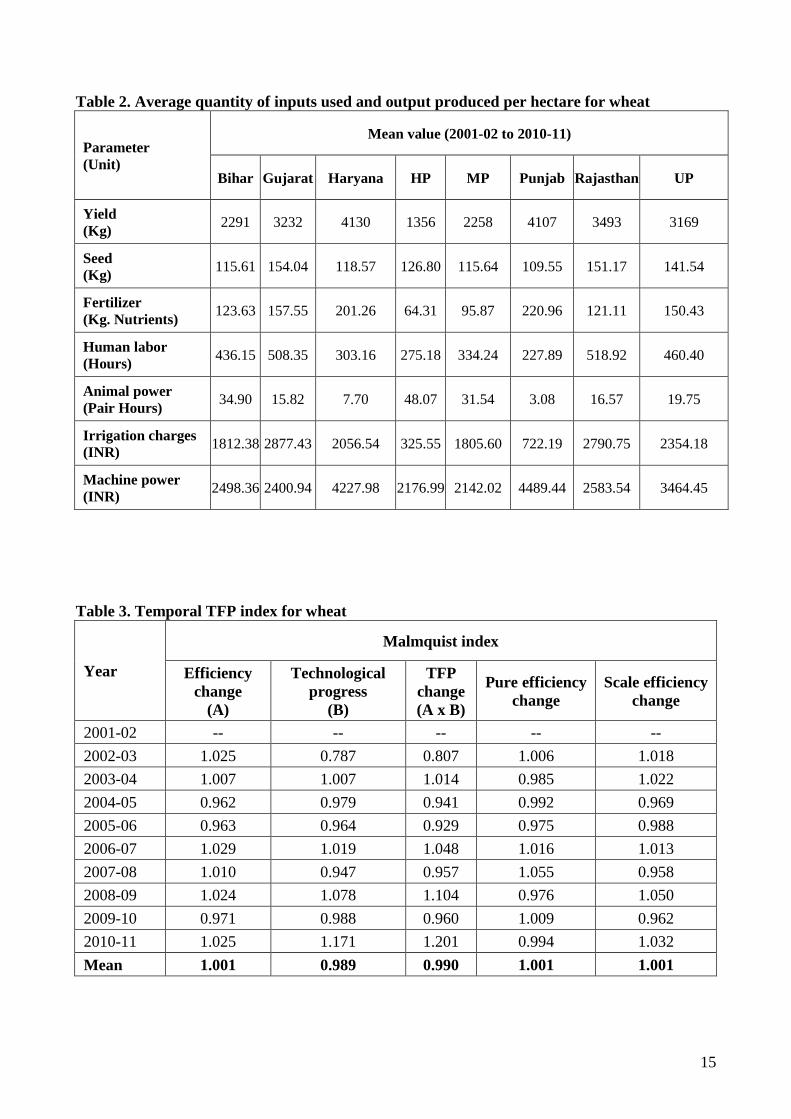
The average quantity of inputs used and output produced is furnished in Table 2. The

highest average productivity registered was in Haryana (4130 Kg/ha) followed by Punjab and

Rajasthan the lowest in Himachal Pradesh (1356 Kg/ha). The seed rate used was more in Gujarat

followed by Rajasthan and Uttar Pradesh. Fertilizer use was more in the productive regions like

Punjab, Haryana and Uttar Pradesh and less in hilly regions like Himachal Pradesh which uses more

of manures. Wheat cultivation is almost wholly mechanized in Punjab and Haryana as indicated by

the share of machine power cost against the high share of animal power cost in Bihar and Himachal

Pradesh.

4.2. Spatial and Temporal Trends in TFP and its Determinants

The total factor productivity change is the product of efficiency and technological change. Index

measures greater (less) than unity indicate that there has been productivity gain (loss), efficiency

increase (decrease) or technological progress (regress). Similarly, the overall efficiency change is

the product of pure technical efficiency and scale efficiency change. Given that the determinants of

MIP change is a multiplicative composite of efficiency and technological change, the major cause

of productivity improvements can be ascertained by comparing the values of the efficiency change

and technological change indexes. Put differently, the productivity improvements described can be

the result of efficiency gains, technological progress, or both (Worthington, 2000). TFP estimates of

the study depict a mixed trend as revealed by the temporal and spatial analysis (Table 3 and 4). The

TFP change varied considerably across the years, with 2002-03, 2004-05, 2005-06, 2007-08 and

2009-10 registering decline in comparison to the base, 2001-02, and the rest exhibited a positive.

Inter alia, the inter-year negative growth shall be attributed to the environmental factors which

sometimes have a detrimental effect on the input usage resulting in yield loss.

8

The positive TFP growth ranged between 1.4 per cent (2003-04) to 20.10 per cent (2010-

11). The highest positive change was noticed in 2010-11 owing to a growth in technological

progress at 17.10 per cent coupled with an increase in efficiency across states by 2.50 per cent in

2010-11 (Table 3). The mean total factor productivity during the period fell by one per cent (0.099

– 1.000). This was composed of a 0.1 per cent efficiency gain (1.001 – 1.000) and a -1.1 per cent

decrease (0.989 – 1.000) due to technological progress. The efficiency change when decomposed

into its pure efficiency and scale efficiency portions indicated 0.1 per cent increase each (1.001 –

1.000).

Overall, the pure efficiency as well as scale efficiency showed a marginal positive change

during the period. A mixed pattern has been found in pure efficiency and scale efficiency for the

decade. For instance, in 2002-03, the efficiency has increased by 2.50 per cent owing to the increase

in pure efficiency (0.6%) as well as scale efficiency (1.8%). But, in 2003-04, efficiency even

though increased by 0.70 per cent, the contribution of scale efficiency (2.2%) countering the fall in

pure efficiency (1.5%). The overall improvement in productivity over the period is composed of an

average efficiency increase (movement towards the frontier) of 0.10 percent, and an average

technological regress (downward shift of the frontier) of 1.0 percent. However, these figures serve

to obscure some variation in productivity for each of the years in the sample. For example, annual

changes in technological progress range from a loss of -21.3 per cent in 2002-03 to a gain of 17.1

per cent in 2010-11, whereas, efficiency change maintains a gain of 2.5 per cent during the same

period.

All the states barring Himachal Pradesh and Uttar Pradesh have been efficient in wheat

production, whereas only Rajasthan seem to have realised the full potential of technological

progress (Table 4). It is noteworthy that the change in efficiency is constant (pure and scale

efficiencies as well) during the decade for all states excluding Bihar, Madhya Pradesh and Uttar

Pradesh. Hence, there exists scope among states to improve their efficiency in terms of inputs use in

varying magnitude. Interestingly, there are two implications arising from this result. One, for

progressive states like Haryana and Punjab which almost reached its potential yield, farmers do

adopt latest technologies and improved wheat production techniques. But the need is developing

technologies that produce more than the current potential yield. Second, specifically for states like

Himachal Pradesh wherein the adoption rate is very low, the TFP can be increased by taking

advantage of the latest available wheat crop management technologies. However, the mean TFP

reveals that at current level of technology, the yield realization seems to have reached a ceiling,

irrespective of the base level. It is an indication that there is an emergent need for technologies that

break the yield barrier.

9

Across states, the pure as well as scale efficiency remains unchanged for a majority of the

states. Analysis on temporal and spatial trends in TFP suggests that the development strategy

should focus attention towards the determinants of TFP viz., efficiency and/or technological

progress. Both efficiency increase and technological progress can be achieved only through

research and extension which needs sufficient funding. Investment in research helps to develop

improved genotypes (shifts the production frontier upward by augmenting the yield) and

technologies or techniques with improved efficiency that uses optimal resources (movement in the

production frontier to the optimal point with increased efficiency in the use of resource/resources

combination). Chand et al. (2011) identified that 19.5 per cent increase in the investment stock for

wheat research in nominal terms, will increase the TFP by one per cent. Investment in wheat

extension activities will help to carry the improved technologies and efficient techniques from lab

to farmer’s field. The following section articulates the strategies for increasing the TFP, an expected

outcome of investment in research and extension.

Perusal of Table 5 indicates that inputs growth (derived by dividing the output growth by

TFP growth) and output growth is positive for all the wheat growing states barring Himachal

Pradesh and Punjab. This indicated the declining trend in output in these two states with two

distinct scenarios. Among others, declining TFP in Himachal Pradesh shall be attributed largely to

the declining growth in inputs followed by output. The strategy here is to transform the negative

output growth to a positive growth through adoption of improved technologies and optimal

allocation of resources to increase the resource-use efficiency. However, in the case of Punjab, an

increased change in the TFP has been noticed despite declining output (-0.76%) and inputs growth

(-0.75%). Here, the variation in magnitude of the growth figures despite carrying a negative sign

helps Punjab to register a positive growth in TFP. The plausible reason might be due to the rational

use/combination of resources particularly with the increased adoption of resource conservation

technologies like zero tillage in the last decade which reduces the cost of production. Yet, Uttar

Pradesh registered a declining TFP trend despite the positive growth in inputs and output. The

reason was growth in composite inputs is higher than the magnitude of the output growth. The

strategy for achieving a positive change in TFP is to use resources in an optimal manner and saving

costs.

Table 6 shows the comparison in growth between production, yield and TFP to draw some

inference supported with the varieties released for different periods. However, there is no clear cut

pattern or cause and effect relation between the selected variables for empirical inference. The TFP

shows a positive association with the number of varieties released during the specific period

justifying investment in research (Chand et al., 2011) and extension. For instance, a record number

10

of genotypes (118 varieties for different agro-climatic regions) have been released during 2001-

2010 (Figure 10) which had a strong impact on the TFP in 2000s. Now, there arises a serious

question how far the TFP is influenced by the number of wheat varieties released in a year? This is

a widely misunderstood and complicated issue to address since the varieties released in a particular

year will take around three years to reach the farmers’ field. Hence, three years lag was maintained

based on the breeding cycle to probe into the influence of released varieties on TFP. Also, growth

in yield and production has been compared with the TFP growth (CAGR) as these are the major

factors that influence the TFP (Table 6). Overall, the study calls for a boost in research investment

aiming at evolving genotypes involving cutting edge sciences that could break the barriers to

potential yield to usher in innovations in terms of technical progress as supported by the data

furnished in Table 7.

5. Conclusions and Policy Implications

Agricultural production is an essentially a biological activity guided by several factors including

weather. Despite higher quantity of inputs used, output produced depends on the technical

efficiency of inputs and adoption of improved technology. Hence, it is essential to constantly

monitor if the productivity growth is area or input or price or technology driven or a combination of

a few of these to formulate appropriate research and price policies. As the interest of the study is to

restrict the analysis to the impact of technology and input efficiency on productivity, the Malmquist

index of TFP has been deployed. The results indicate that the overall TFP change is marginally

negative in wheat during the period restricting the technical progress realization to certain years and

regions. Additional productivity is a result of increased and efficient use of inputs. The results

indicate that the technology stabilization is yet to become more robust to insulate wheat productive

performances from biotic and abiotic factor’s negative influence. The policy prescription calls for a

differential treatment with higher investment on research to harness new sciences in breaking the

yield barrier in traditional wheat growing states barring Uttar Pradesh combined with sustainable

cultivation practices for efficient input use. Himachal Pradesh needs measures to shift frontiers and

efficiency. Many states have posted constant technical efficiency calling for strengthening the

research on appropriate technologies in natural resource management for increasing the input use

efficiency and levels or minimising the costs.

11

References

Alene, A. D., 2009. Productivity Growth and the Effects of Research and Development in African

Agriculture, Contributed paper prepared for the presentation at the International Association of

Agricultural Economists Conference, Beijing, China, August 16-22.

Arnade, C., 1998. Using a programming approach to measure international agricultural efficiency

and productivity, J. Agric. Econ. 49, 67-84.

Baset, M. A., Karim, M. R., M. Akter, 2009. Measurement and analysis of total factor productivity

growth in modern variety potato, J. Agric. Rural Dev. 7 (1 and 2): 65 - 71.

Bhushan, S., 2005. Total factor productivity growth of wheat in India: A Malmquist approach, Ind.

J. Agric. Econ. 60 (1).

Caves, D.W., Christensen, L.R., Diewert, W.E., 1982. The economic theory of index numbers and

the measurement of input, output and productivity, Econometrica. 1393-1414.

Chand, R., Kumar, P., S. Kumar, 2012. Total factor productivity and returns to public investment

on agricultural research in India, Agric. Econ. Res. Rev. 25(2), 181-194.

Chand, R., Kumar, P., S. Kumar, 2011. Total Factor Productivity and Contribution of Research

Investment to Agricultural Growth in India, National Centre for Agricultural Economic and Policy

Research, Policy Paper 25. March 2011.

Charnes, A., Cooper, W. W., Rhodes, E., 1978. Measuring the efficiency of decision making units.

Euro. J. Operations Research. 2, 429-444.

Chaudhary, S., 2012. Trends in Total Factor Productivity in Indian Agriculture: State Level

Evidence Using Non-Parametric Sequential Malmquist Index. Working Paper No. 215, Center for

Development Economics, Department of Economics, Delhi School of Economics.

Christensen, L. R., 1975. Concepts and measurement of agricultural productivity, Am. J. Agric.

Econ. 57 (5), 910-15.

Coelli, T. J., 1996. A Guide to DEAP Version 2.1: A Data Envelopment Analysis (Computer

Program), Centre for Efficiency and Productivity Analysis, University of New England, Australia.

12

Coelli, T. J., D. S. P. Rao, 2003. Total Factor Productivity Growth in Agriculture: A Malmquist

Index Analysis of 93 Countries1980-2000, Centre for Efficiency and Productivity Analysis,

Working Paper Series, No. 02/2003, School of Economics, University of Queensland Australia.

Coelli, T. J., Rahman, S., T. Colin, 2003. A stochastic frontier approach to total factor productivity

measurement in Bangladesh crop agriculture, J. Int. Dev. 15, 321-333.

Diewert, W. E., 1976. Exact and superlative index numbers. J. Econometrics. 4 (2), 115-45.

Fare, R., Grosskopf, S., Norris, M., Zhang, Z., 1994. Productivity growth, technical progress, and

efficiency change in industrialised countries. T. Am. Eco. Rev. 66-83.

Farrell, M. J., 1957. The measurement of productive efficiency. J. Royal Stat. Soc. Ser. A

(General). Part 3, 120, 253-290.

Forstner, H., A. Isaksson, 2002. Productivity, Technology, and Efficiency: An Analysis of the

World Technology Frontier when Memory is Infinite, SIN Working Paper Series, Working Paper

No. 7, February 2002, Statistics and Information Networks branch of UNIDO.

Fulginiti, L. E., R. K. Perrin, 1998. Agricultural productivity in developing countries, Agric. Econ.

19, 45-51.

Grosskopf, S., 1993. Efficiency and Productivity, in O.H.Fried, C.A.K.Lovell and S.S. Schimdt,

eds., The Measurement of Productivity Efficiency. Oxford University Press, New York.

Gujarati, D. N., 2003. Basic Econometrics. McGraw Hill, New York.

Hayami, Y., Kikuchi, M., 1999. The three decades of green revolution in a Philippine village. Jap.

J. Rural Econ. 1, 10-24.

Kannan, E., 2011. Total Factor Productivity Growth and its Determinants in Karnataka Agriculture,

Working Paper: 265, The Institute for Social and Economic Change, Bangalore.

Kumar, P. and M. W. Rosegrant, 1994. Productivity and sources of growth for rice in India, Eco.

and Pol. Weekly. December 31, 1994, p A-183 to A-188.

Kumar, P. and Mruthyunjaya, 1992. Measurement and analysis of total factor productivity growth

in wheat, Ind. J. Agric. Econ. 47(7), 451-458.

13

Kumar, P., 2001. Agricultural performance and productivity, in S.S.Acharya and D.P.Chaudhri,

eds., Indian Agricultural Policy at the Crossroads. Rawat Publications, New Delhi.

Kumar, P., S. Mittal, 2006. Agricultural productivity trends in India: Sustainability issues, Agric.

Econ. Res. Rev. 19, 71-88.

Murgai, R., 1999. The Green Revolution and the Productivity Paradox- Evidence from the Indian

Punjab, Policy Research Working Paper 2234, The World Bank Development Research Group,

Rural Development, November 1999.

Murgai, R., 2005. The green revolution and productivity paradox: Evidence from Indian Punjab.

Agric. Econ. 25 (2-3), 199-209.

Narayanamoorthy, A., 2007. Deceleration in agricultural growth: Technology or policy fatigue.

Eco. and Pol. Weekly. 42(25), 2375-79.

Nin, A., Channing, A., V. P. Paul, 2003. Is Agricultural Productivity in Developing Countries really

Shrinking? New Evidence Using a Modified Nonparametric Approach, J. Dev. Econ. 71, 395-415.

Rahman, S., 2004. Regional Productivity and Convergence in Bangladesh Agriculture, Paper

presented at the Annual Meeting of the American Agric. Econ. Association held in Aug 1-4, 2004,

Project MUSE Scholarly Journals Online.

Ray, D. K., N. D. Mueller, P. C. West, J. A. Foley, 2013. Yield trends are insufficient to double

global crop production by 2050. Plos One. 8, 66428.

Sendhil, R., Randhir Singh, Indu Sharma, 2012. Exploring the performance of wheat production in

India. J. Wheat Res. 4 (2), 37-44.

Sidhu, D. S., D. Byerlee, 1992. Technical Change and Wheat Productivity in the Indian Punjab in

Post-GR Period. Working Paper 92-02, CIMMYT, Mexico.

Trueblood, M. A., 1996. An Intercountry Comparison of Agricultural Efficiency and Productivity,

Ph.D dissertation, University of Minnesota.

Worthington, A., 2000. Technical efficiency and technological change in Australian building

societies. Abacus. 36(2), 180-197.

14

Table 1. Estimated growth in inputs used and output produced from 2001-02 to 2010-11

Parameters Positive growth (CAGR in %) Negative growth (CAGR in %)

Output Madhya Pradesh (4.12)

Gujarat (1.40)

Bihar (1.40)

Rajasthan (1.31)

Uttar Pradesh (1.24)

Haryana (1.15)

Himachal Pradesh (-1.16)

Punjab (-0.76)

Seed rate

Gujarat (0.26)

Punjab (0.92)

Rajasthan (0.23)

Bihar (-0.63)

Haryana (-0.50)


Madhya Pradesh (-0.04)

Uttar Pradesh (-0.19)

Fertilizer

Gujarat (2.71)

Haryana (0.59)

Himachal Pradesh (1.65)

Madhya Pradesh (2.44)

Rajasthan (2.98)


Bihar (-0.02)

Punjab (-0.29)

Human labour

Uttar Pradesh (0.10) Bihar (-1.62)

Gujarat (-6.39)

Haryana (-0.30)



Punjab (-1.20)

Rajasthan (-3.12)

Animal power

-- Bihar (-7.13)

Gujarat (-8.55)

Haryana (-12.94)



Punjab (-2.14)

Rajasthan (-10.82)

Uttar Pradesh (-9.01)

Irrigation charges Bihar (6.21)

Gujarat (3.43)

Haryana (4.83)



Punjab (0.96)

Rajasthan (0.42)


--

Machine power Bihar (6.96)

Gujarat (8.89)

Haryana (8.06)



Punjab (7.91)

Rajasthan (8.85)


--

15

Table 2. Average quantity of inputs used and output produced per hectare for wheat

Parameter

(Unit)

Mean value (2001-02 to 2010-11)

Bihar Gujarat Haryana HP MP Punjab Rajasthan UP

Yield

(Kg) 2291 3232 4130 1356 2258 4107 3493 3169

Seed

(Kg) 115.61 154.04 118.57 126.80 115.64 109.55 151.17 141.54

Fertilizer

(Kg. Nutrients) 123.63 157.55 201.26 64.31 95.87 220.96 121.11 150.43

Human labor

(Hours) 436.15 508.35 303.16 275.18 334.24 227.89 518.92 460.40

Animal power

(Pair Hours) 34.90 15.82 7.70 48.07 31.54 3.08 16.57 19.75

Irrigation charges

(INR) 1812.38 2877.43 2056.54 325.55 1805.60 722.19 2790.75 2354.18

Machine power

(INR) 2498.36 2400.94 4227.98 2176.99 2142.02 4489.44 2583.54 3464.45

Table 3. Temporal TFP index for wheat

Year

Malmquist index

Efficiency

change

(A)

Technological

progress

(B)

TFP

change

(A x B)

Pure efficiency

change

Scale efficiency

change

2001-02 -- -- -- -- --

2002-03 1.025 0.787 0.807 1.006 1.018

2003-04 1.007 1.007 1.014 0.985 1.022

2004-05 0.962 0.979 0.941 0.992 0.969

2005-06 0.963 0.964 0.929 0.975 0.988

2006-07 1.029 1.019 1.048 1.016 1.013

2007-08 1.010 0.947 0.957 1.055 0.958

2008-09 1.024 1.078 1.104 0.976 1.050

2009-10 0.971 0.988 0.960 1.009 0.962

2010-11 1.025 1.171 1.201 0.994 1.032

Mean 1.001 0.989 0.990 1.001 1.001

16

Table 4. Spatial TFP index for wheat

State

Malmquist index

Efficiency

change

(A)

Technological

progress

(B)

TFP change

(A x B)

Pure

efficiency

change

Scale

efficiency

change

Bihar 1.010 1.005 1.016 1.024 0.986

Gujarat 1.000 1.013 1.013 1.000 1.000

Haryana 1.000 1.022 1.022 1.000 1.000

Himachal Pradesh 1.000 0.835 0.835 1.000 1.000

Madhya Pradesh 1.016 1.001 1.017 1.000 1.016

Punjab 1.000 1.016 1.016 1.000 1.000

Rajasthan 1.000 1.024 1.024 1.000 1.000

Uttar Pradesh 0.985 1.007 0.922 0.981 1.004

Mean 1.001 0.989 0.990 1.001 1.001

Table 5. Output and inputs growth vis-à-vis TFP growth

State TFP change Output growth (%) Inputs growth (%)

Bihar 1.016 1.40 1.38

Gujarat 1.013 1.40 1.38

Haryana 1.022 1.15 1.13

Himachal Pradesh 0.835 -1.16 -1.39

Madhya Pradesh 1.017 4.12 4.05

Punjab 1.016 -0.76 -0.75

Rajasthan 1.024 1.31 1.28

Uttar Pradesh 0.922 1.24 1.25

Table 6. Comparison of CAGR in production, yield, TFP and number of varieties released

Period CAGR in %

Number of varieties released* Production Yield TFP

1960s 6.82 4.46 N.E. 28 (from 1965)

1970s 4.31 1.87 N.E. 69

1980s 3.58 3.10 1.49^ 89

1990s 3.57 1.82 0.34^ 78

2000s 1.90 0.69 2.12 118

Note: Data compiled from ^Bhushan (2005), Sendhil et al. (2012) and ICAR-IIWBR, Karnal (India).

N.E indicates the non-estimation of the TFP due to non-availability of input use data in the early 70s.

* indicate the number of wheat varieties released by the State and Central Varietal Release Committee.

17

Table 7. Comparison of potential yield, average yield of the released wheat varieties in India

Period

Number of

varieties

released

Potential yield

(tonnes/hectare)

Average yield

(tonnes/hectare)

Difference between potential and

average yield

(tonnes/hectare)

1961 to 1970 28

(from 1965) 3.65 2.43 1.22

1971 to 1980 69 3.77

(3.43)

3.03

(24.54) 0.74

1981 to 1990 89 4.24

(12.30)

3.28

(8.16) 0.96

1991 to 2000 78 4.42

(4.26)

3.65

(11.35) 0.77

2001 to 2010 118 5.00

(13.24)

3.90

(6.77) 1.11

Note: Figures within parenthesis in column 3 and 4 indicate the per cent change over previous year estimates. Potential

yield is the maximum yield obtained in an experimental site during the three year trails across the country. It is

averaged and presented in the column 3. The average yield in column 4 is the mean of all varieties yield across sites and

years for the selected period.

18

Figure 1. Production possibility set for period t and t+1

Figure 2. Output and inputs trend for wheat in Bihar

Figure 3. Output and inputs trend for wheat in Gujarat

INPUTS YIELD

INPUTS YIELD

19

Figure 4. Output and inputs trend for wheat in Haryana

Figure 5. Output and inputs trend for wheat in Himachal Pradesh

Figure 6. Output and inputs trend for wheat in Madhya Pradesh

INPUTS YIELD

INPUTS YIELD

INPUTS YIELD

20

Figure 7. Output and inputs trend for wheat in Punjab

Figure 8. Output and inputs trend for wheat in Rajasthan

Figure 9. Output and inputs trend for wheat in Uttar Pradesh

INPUTS YIELD

INPUTS YIELD

INPUTS YIELD

21

Note: 118 varieties were released during 2000-01 to 2010-11. However, only a few varieties are visible in X-axis by default.

Figures within square brackets indicate the year of release and text within normal parenthesis indicates the local name.

Figure 10. Trend in potential yield of released varieties during 2000-01 to 2010-11

Potential yield in tonnes/hectare

trends and determinants of research driven total...

Documents