transmission network fault location observability with minimal pmu placement

1128 IEEE TRANSACTIONS ON POWER DELIVERY, VOL. 21, NO. 3, JULY 2006

Transmission Network Fault Location ObservabilityWith Minimal PMU Placement

Kai-Ping Lien, Student Member, IEEE, Chih-Wen Liu, Senior Member, IEEE, Chi-Shan Yu, Member, IEEE, andJoe-Air Jiang, Member, IEEE

Abstract—This paper presents a concept of fault-location ob-servability and a new fault-location scheme for transmission net-works based on synchronized phasor measurement units (PMUs).Using the proposed scheme, minimal PMUs are installed in existingpower transmission networks so that the fault, if it occurs, can belocated correctly in the network. The scheme combines the fault-lo-cation algorithm and the fault-side selector. Extensive simulationresults verify the proposed scheme.

Index Terms—Fault location, phasor measurement unit (PMU),transmission network.

I. INTRODUCTION

ACCURATE estimate of the fault location is critical to in-spection, maintenance, and repair of transmission lines

[1]–[8]. Several two-terminal fault-location algorithms based onphasor measurement units (PMUs) techniques have been pro-posed [9]–[13] recently. These PMU-based algorithms proposethe calculation of fault location using synchronized voltage andcurrent phasors. While they can achieve high accuracy in faultlocation, they are limited to locate faults in a transmission net-work installed by PMUs on every bus. Considering the installa-tion cost of PMUs, it is important to investigate the placementscheme of the PMUs at minimal locations on the network in thesense that the fault-location observability can be achieved overthe entire network. By borrowing from the concept of networkstate observability, which means that the entire steady-state busvoltage phasors can be estimated using the installed meter mea-surements, we define the fault-location observability as that if afault occurs on the network, then it can be located exactly usingthe installed digital fault recorders such as PMUs.

Based on the topology of the power system, this paper firstproposes a minimal placement strategy of PMUs, and thendevelops an innovative fault-location algorithm for the trans-mission network. Using installed PMUs, the new fault-locationscheme can enhance the protection function of the network.In the proposed scheme, every line section in transmissionnetworks only needs one-side PMU installation. The proposed

Manuscript received February 3, 2005; revised May 26, 2005. This work wassupported by the National Science Council of Taiwan, R.O.C., under ContractNSC-93-2213-E-002-054. Paper no. TPWRD-00067-2005.

K.-P. Lien and C.-W. Liu are with the Department of Electrical En-gineering, National Taiwan University, Taipei 106, Taiwan (e-mail:[email protected], [email protected]).

C.-S. Yu is with the National Defense University, Chung-Cheng Institute ofTechnology, Taoyuan 335, Taiwan (e-mail: [email protected]).

J.-A. Jiang is with the Department of Bio-Industrial Mechatronics Engi-neering, National Taiwan University, Taipei 106, Taiwan, R.O.C. (e-mail:[email protected]).

Digital Object Identifier 10.1109/TPWRD.2005.858806

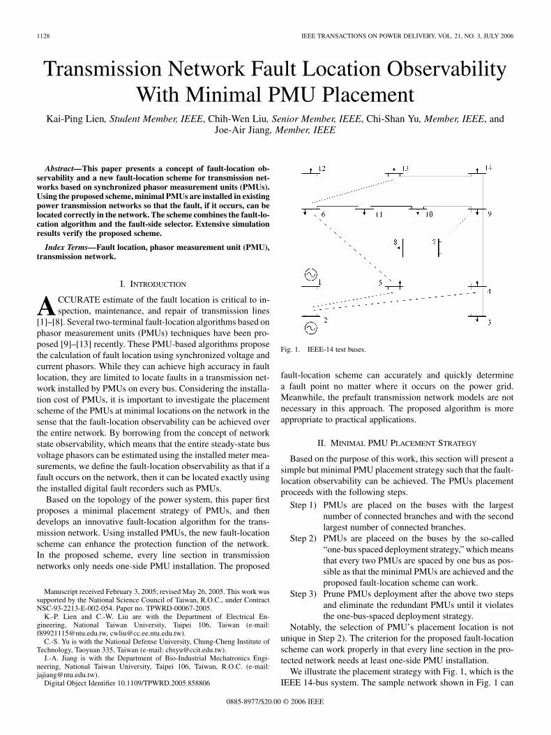
Fig. 1. IEEE-14 test buses.

fault-location scheme can accurately and quickly determinea fault point no matter where it occurs on the power grid.Meanwhile, the prefault transmission network models are notnecessary in this approach. The proposed algorithm is moreappropriate to practical applications.

II. MINIMAL PMU PLACEMENT STRATEGY

Based on the purpose of this work, this section will present asimple but minimal PMU placement strategy such that the fault-location observability can be achieved. The PMUs placementproceeds with the following steps.

Step 1) PMUs are placed on the buses with the largestnumber of connected branches and with the secondlargest number of connected branches.

Step 2) PMUs are placeed on the buses by the so-called“one-bus spaced deployment strategy,” which meansthat every two PMUs are spaced by one bus as pos-sible as that the minimal PMUs are achieved and theproposed fault-location scheme can work.

Step 3) Prune PMUs deployment after the above two stepsand eliminate the redundant PMUs until it violatesthe one-bus-spaced deployment strategy.

Notably, the selection of PMU’s placement location is notunique in Step 2). The criterion for the proposed fault-locationscheme can work properly in that every line section in the pro-tected network needs at least one-side PMU installation.

We illustrate the placement strategy with Fig. 1, which is theIEEE 14-bus system. The sample network shown in Fig. 1 can

0885-8977/$20.00 © 2006 IEEE

LIEN et al.: TRANSMISSION NETWORK FAULT LOCATION OBSERVABILITY 1129

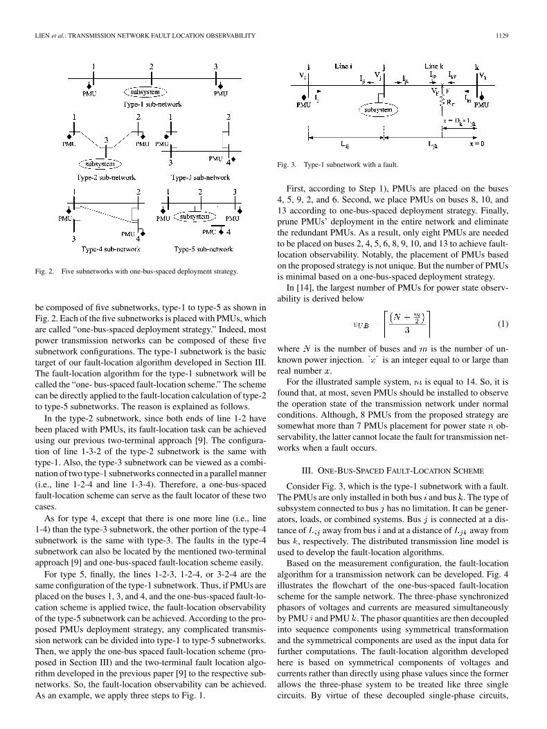
Fig. 2. Five subnetworks with one-bus-spaced deployment strategy.

be composed of five subnetworks, type-1 to type-5 as shown inFig. 2. Each of the five subnetworks is placed with PMUs, whichare called “one-bus-spaced deployment strategy.” Indeed, mostpower transmission networks can be composed of these fivesubnetwork configurations. The type-1 subnetwork is the basictarget of our fault-location algorithm developed in Section III.The fault-location algorithm for the type-1 subnetwork will becalled the “one- bus-spaced fault-location scheme.” The schemecan be directly applied to the fault-location calculation of type-2to type-5 subnetworks. The reason is explained as follows.

In the type-2 subnetwork, since both ends of line 1-2 havebeen placed with PMUs, its fault-location task can be achievedusing our previous two-terminal approach [9]. The configura-tion of line 1-3-2 of the type-2 subnetwork is the same withtype-1. Also, the type-3 subnetwork can be viewed as a combi-nation of two type-1 subnetworks connected in a parallel manner(i.e., line 1-2-4 and line 1-3-4). Therefore, a one-bus-spacedfault-location scheme can serve as the fault locator of these twocases.

As for type 4, except that there is one more line (i.e., line1-4) than the type-3 subnetwork, the other portion of the type-4subnetwork is the same with type-3. The faults in the type-4subnetwork can also be located by the mentioned two-terminalapproach [9] and one-bus-spaced fault-location scheme easily.

For type 5, finally, the lines 1-2-3, 1-2-4, or 3-2-4 are thesame configuration of the type-1 subnetwork. Thus, if PMUs areplaced on the buses 1, 3, and 4, and the one-bus-spaced fault-lo-cation scheme is applied twice, the fault-location observabilityof the type-5 subnetwork can be achieved. According to the pro-posed PMUs deployment strategy, any complicated transmis-sion network can be divided into type-1 to type-5 subnetworks.Then, we apply the one-bus spaced fault-location scheme (pro-posed in Section III) and the two-terminal fault location algo-rithm developed in the previous paper [9] to the respective sub-networks. So, the fault-location observability can be achieved.As an example, we apply three steps to Fig. 1.

Fig. 3. Type-1 subnetwork with a fault.

First, according to Step 1), PMUs are placed on the buses4, 5, 9, 2, and 6. Second, we place PMUs on buses 8, 10, and13 according to one-bus-spaced deployment strategy. Finally,prune PMUs’ deployment in the entire network and eliminatethe redundant PMUs. As a result, only eight PMUs are neededto be placed on buses 2, 4, 5, 6, 8, 9, 10, and 13 to achieve fault-location observability. Notably, the placement of PMUs basedon the proposed strategy is not unique. But the number of PMUsis minimal based on a one-bus-spaced deployment strategy.

In [14], the largest number of PMUs for power state observ-ability is derived below

(1)

where is the number of buses and is the number of un-known power injection. is an integer equal to or large thanreal number .

For the illustrated sample system, is equal to 14. So, it isfound that, at most, seven PMUs should be installed to observethe operation state of the transmission network under normalconditions. Although, 8 PMUs from the proposed strategy aresomewhat more than 7 PMUs placement for power state ob-servability, the latter cannot locate the fault for transmission net-works when a fault occurs.

III. ONE-BUS-SPACED FAULT-LOCATION SCHEME

Consider Fig. 3, which is the type-1 subnetwork with a fault.The PMUs are only installed in both bus and bus . The type ofsubsystem connected to bus has no limitation. It can be gener-ators, loads, or combined systems. Bus is connected at a dis-tance of away from bus and at a distance of away frombus , respectively. The distributed transmission line model isused to develop the fault-location algorithms.

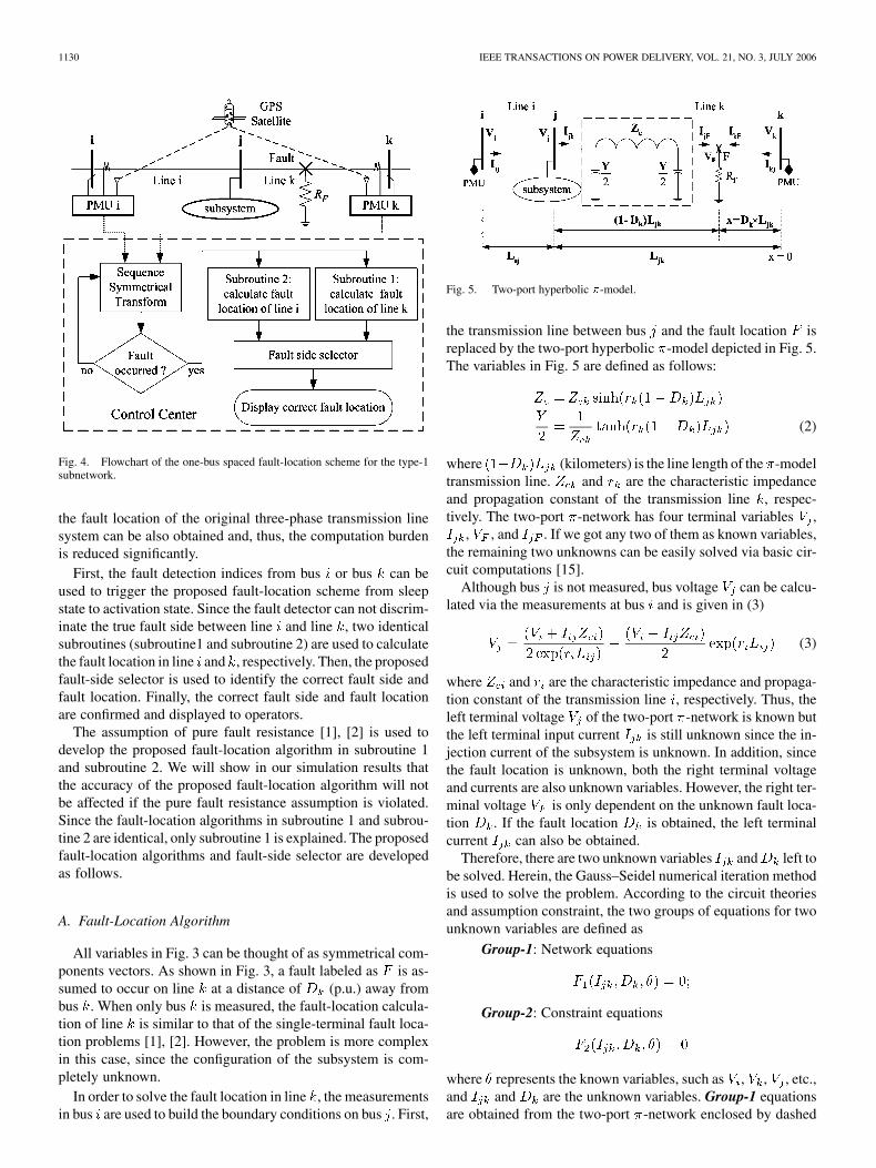
Based on the measurement configuration, the fault-locationalgorithm for a transmission network can be developed. Fig. 4illustrates the flowchart of the one-bus-spaced fault-locationscheme for the sample network. The three-phase synchronizedphasors of voltages and currents are measured simultaneouslyby PMU and PMU . The phasor quantities are then decoupledinto sequence components using symmetrical transformationand the symmetrical components are used as the input data forfurther computations. The fault-location algorithm developedhere is based on symmetrical components of voltages andcurrents rather than directly using phase values since the formerallows the three-phase system to be treated like three singlecircuits. By virtue of these decoupled single-phase circuits,


Fig. 4. Flowchart of the one-bus spaced fault-location scheme for the type-1subnetwork.

the fault location of the original three-phase transmission linesystem can be also obtained and, thus, the computation burdenis reduced significantly.

First, the fault detection indices from bus or bus can beused to trigger the proposed fault-location scheme from sleepstate to activation state. Since the fault detector can not discrim-inate the true fault side between line and line , two identicalsubroutines (subroutine1 and subroutine 2) are used to calculatethe fault location in line and , respectively. Then, the proposedfault-side selector is used to identify the correct fault side andfault location. Finally, the correct fault side and fault locationare confirmed and displayed to operators.

The assumption of pure fault resistance [1], [2] is used todevelop the proposed fault-location algorithm in subroutine 1and subroutine 2. We will show in our simulation results thatthe accuracy of the proposed fault-location algorithm will notbe affected if the pure fault resistance assumption is violated.Since the fault-location algorithms in subroutine 1 and subrou-tine 2 are identical, only subroutine 1 is explained. The proposedfault-location algorithms and fault-side selector are developedas follows.

A. Fault-Location Algorithm

All variables in Fig. 3 can be thought of as symmetrical com-ponents vectors. As shown in Fig. 3, a fault labeled as is as-sumed to occur on line at a distance of (p.u.) away frombus . When only bus is measured, the fault-location calcula-tion of line is similar to that of the single-terminal fault loca-tion problems [1], [2]. However, the problem is more complexin this case, since the configuration of the subsystem is com-pletely unknown.

In order to solve the fault location in line , the measurementsin bus are used to build the boundary conditions on bus . First,

Fig. 5. Two-port hyperbolic �-model.

the transmission line between bus and the fault location isreplaced by the two-port hyperbolic -model depicted in Fig. 5.The variables in Fig. 5 are defined as follows:

(2)

where (kilometers) is the line length of the -modeltransmission line. and are the characteristic impedanceand propagation constant of the transmission line , respec-tively. The two-port -network has four terminal variables ,

, , and . If we got any two of them as known variables,the remaining two unknowns can be easily solved via basic cir-cuit computations [15].

Although bus is not measured, bus voltage can be calcu-lated via the measurements at bus and is given in (3)

(3)

where and are the characteristic impedance and propaga-tion constant of the transmission line , respectively. Thus, theleft terminal voltage of the two-port -network is known butthe left terminal input current is still unknown since the in-jection current of the subsystem is unknown. In addition, sincethe fault location is unknown, both the right terminal voltageand currents are also unknown variables. However, the right ter-minal voltage is only dependent on the unknown fault loca-tion . If the fault location is obtained, the left terminalcurrent can also be obtained.

Therefore, there are two unknown variables and left tobe solved. Herein, the Gauss–Seidel numerical iteration methodis used to solve the problem. According to the circuit theoriesand assumption constraint, the two groups of equations for twounknown variables are defined as

Group-1: Network equations

Group-2: Constraint equations

where represents the known variables, such as , , , etc.,and and are the unknown variables. Group-1 equationsare obtained from the two-port -network enclosed by dashed


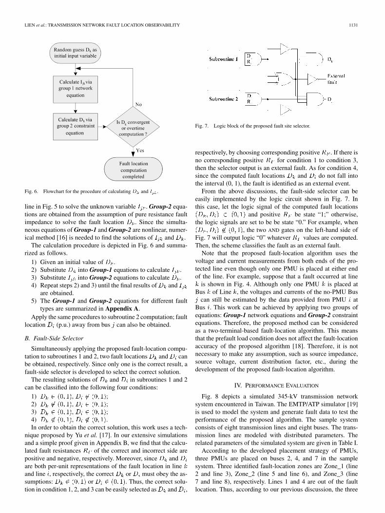
Fig. 6. Flowchart for the procedure of calculating D and I .

line in Fig. 5 to solve the unknown variable . Group-2 equa-tions are obtained from the assumption of pure resistance faultimpedance to solve the fault location . Since the simulta-neous equations of Group-1 and Group-2 are nonlinear, numer-ical method [16] is needed to find the solutions of and .

The calculation procedure is depicted in Fig. 6 and summa-rized as follows.

1) Given an initial value of .2) Substitute into Group-1 equations to calculate .3) Substitute into Group-2 equations to calculate .4) Repeat steps 2) and 3) until the final results of and

are obtained.5) The Group-1 and Group-2 equations for different fault

types are summarized in Appendix A.Apply the same procedures to subroutine 2 computation; fault

location (p.u.) away from bus can also be obtained.

B. Fault-Side Selector

Simultaneously applying the proposed fault-location compu-tation to subroutines 1 and 2, two fault locations and canbe obtained, respectively. Since only one is the correct result, afault-side selector is developed to select the correct solution.

The resulting solutions of and in subroutines 1 and 2can be classified into the following four conditions:

1) , ;2) , ;3) , ;4) , .In order to obtain the correct solution, this work uses a tech-

nique proposed by Yu et al. [17]. In our extensive simulationsand a simple proof given in Appendix B, we find that the calcu-lated fault resistances of the correct and incorrect side arepositive and negative, respectively. Moreover, since andare both per-unit representations of the fault location in lineand line , respectively, the correct or must obey the as-sumptions: or . Thus, the correct solu-tion in condition 1, 2, and 3 can be easily selected as and ,

Fig. 7. Logic block of the proposed fault site selector.

respectively, by choosing corresponding positive . If there isno corresponding positive for condition 1 to condition 3,then the selector output is an external fault. As for condition 4,since the computed fault locations and do not fall intothe interval (0, 1), the fault is identified as an external event.

From the above discussions, the fault-side selector can beeasily implemented by the logic circuit shown in Fig. 7. Inthis case, let the logic signal of the computed fault locations

and positive be state “1;” otherwise,the logic signals are set to be be state “0.” For example, when

, the two AND gates on the left-hand side ofFig. 7 will output logic “0” whatever values are computed.Then, the scheme classifies the fault as an external fault.

Note that the proposed fault-location algorithm uses thevoltage and current measurements from both ends of the pro-tected line even though only one PMU is placed at either endof the line. For example, suppose that a fault occurred at line

is shown in Fig. 4. Although only one PMU is placed atBus of Line , the voltages and currents of the no-PMU Bus

can still be estimated by the data provided from PMU atBus . This work can be achieved by applying two groups ofequations: Group-1 network equations and Group-2 constraintequations. Therefore, the proposed method can be consideredas a two-terminal-based fault-location algorithm. This meansthat the prefault load condition does not affect the fault-locationaccuracy of the proposed algorithm [18]. Therefore, it is notnecessary to make any assumption, such as source impedance,source voltage, current distribution factor, etc., during thedevelopment of the proposed fault-location algorithm.

IV. PERFORMANCE EVALUATION

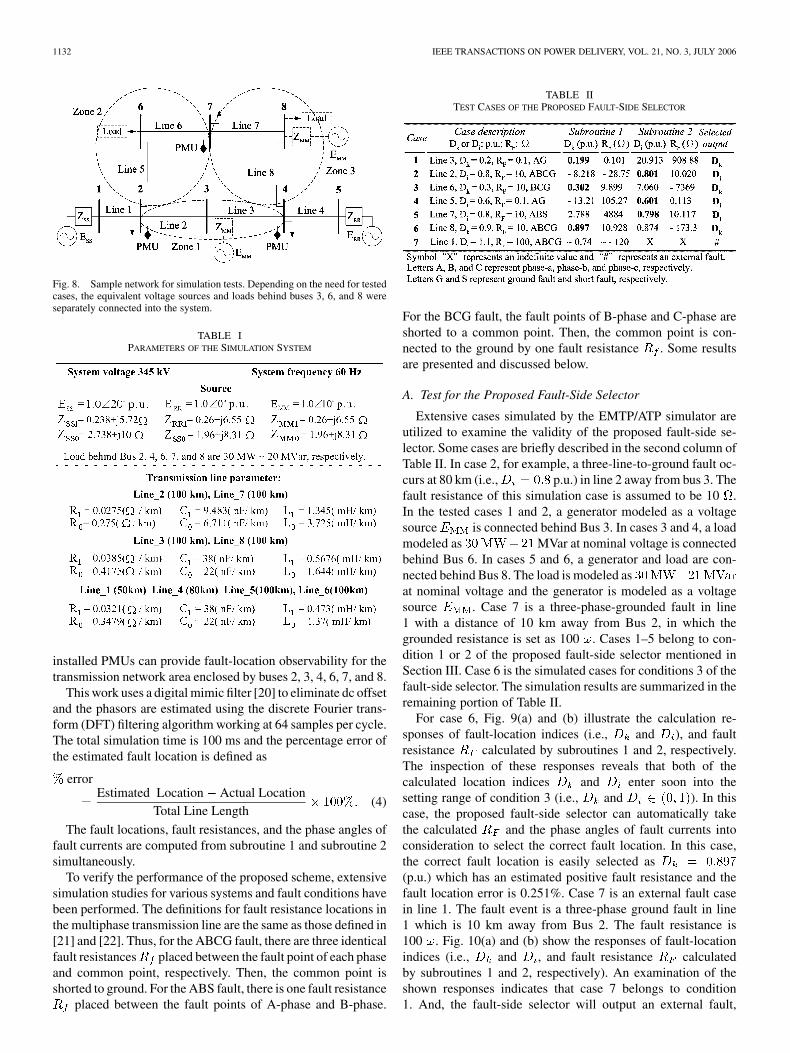
Fig. 8 depicts a simulated 345-kV transmission networksystem encountered in Taiwan. The EMTP/ATP simulator [19]is used to model the system and generate fault data to test theperformance of the proposed algorithm. The sample systemconsists of eight transmission lines and eight buses. The trans-mission lines are modeled with distributed parameters. Therelated parameters of the simulated system are given in Table I.

According to the developed placement strategy of PMUs,three PMUs are placed on buses 2, 4, and 7 in the samplesystem. Three identified fault-location zones are Zone_1 (line2 and line 3), Zone_2 (line 5 and line 6), and Zone_3 (line7 and line 8), respectively. Lines 1 and 4 are out of the faultlocation. Thus, according to our previous discussion, the three


Fig. 8. Sample network for simulation tests. Depending on the need for testedcases, the equivalent voltage sources and loads behind buses 3, 6, and 8 wereseparately connected into the system.

TABLE IPARAMETERS OF THE SIMULATION SYSTEM

installed PMUs can provide fault-location observability for thetransmission network area enclosed by buses 2, 3, 4, 6, 7, and 8.

This work uses a digital mimic filter [20] to eliminate dc offsetand the phasors are estimated using the discrete Fourier trans-form (DFT) filtering algorithm working at 64 samples per cycle.The total simulation time is 100 ms and the percentage error ofthe estimated fault location is defined as

errorEstimated Location Actual Location

Total Line Length(4)

The fault locations, fault resistances, and the phase angles offault currents are computed from subroutine 1 and subroutine 2simultaneously.

To verify the performance of the proposed scheme, extensivesimulation studies for various systems and fault conditions havebeen performed. The definitions for fault resistance locations inthe multiphase transmission line are the same as those defined in[21] and [22]. Thus, for the ABCG fault, there are three identicalfault resistances placed between the fault point of each phaseand common point, respectively. Then, the common point isshorted to ground. For the ABS fault, there is one fault resistance

placed between the fault points of A-phase and B-phase.

TABLE IITEST CASES OF THE PROPOSED FAULT-SIDE SELECTOR

For the BCG fault, the fault points of B-phase and C-phase areshorted to a common point. Then, the common point is con-nected to the ground by one fault resistance . Some resultsare presented and discussed below.

A. Test for the Proposed Fault-Side Selector

Extensive cases simulated by the EMTP/ATP simulator areutilized to examine the validity of the proposed fault-side se-lector. Some cases are briefly described in the second column ofTable II. In case 2, for example, a three-line-to-ground fault oc-curs at 80 km (i.e., p.u.) in line 2 away from bus 3. Thefault resistance of this simulation case is assumed to be 10 .In the tested cases 1 and 2, a generator modeled as a voltagesource is connected behind Bus 3. In cases 3 and 4, a loadmodeled as MVar at nominal voltage is connectedbehind Bus 6. In cases 5 and 6, a generator and load are con-nected behind Bus 8. The load is modeled asat nominal voltage and the generator is modeled as a voltagesource . Case 7 is a three-phase-grounded fault in line1 with a distance of 10 km away from Bus 2, in which thegrounded resistance is set as 100 . Cases 1–5 belong to con-dition 1 or 2 of the proposed fault-side selector mentioned inSection III. Case 6 is the simulated cases for conditions 3 of thefault-side selector. The simulation results are summarized in theremaining portion of Table II.

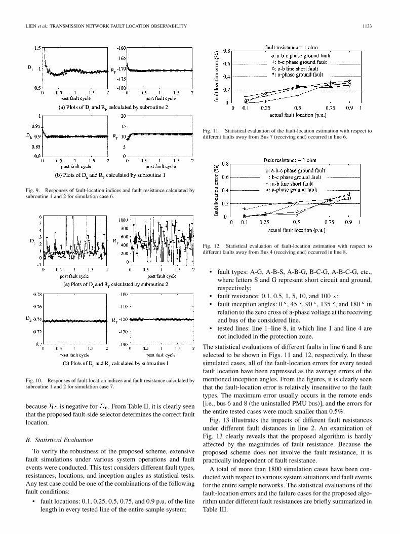
For case 6, Fig. 9(a) and (b) illustrate the calculation re-sponses of fault-location indices (i.e., and ), and faultresistance calculated by subroutines 1 and 2, respectively.The inspection of these responses reveals that both of thecalculated location indices and enter soon into thesetting range of condition 3 (i.e., and ). In thiscase, the proposed fault-side selector can automatically takethe calculated and the phase angles of fault currents intoconsideration to select the correct fault location. In this case,the correct fault location is easily selected as(p.u.) which has an estimated positive fault resistance and thefault location error is 0.251%. Case 7 is an external fault casein line 1. The fault event is a three-phase ground fault in line1 which is 10 km away from Bus 2. The fault resistance is100 . Fig. 10(a) and (b) show the responses of fault-locationindices (i.e., and , and fault resistance calculatedby subroutines 1 and 2, respectively). An examination of theshown responses indicates that case 7 belongs to condition1. And, the fault-side selector will output an external fault,


Fig. 9. Responses of fault-location indices and fault resistance calculated bysubroutine 1 and 2 for simulation case 6.

Fig. 10. Responses of fault-location indices and fault resistance calculated bysubroutine 1 and 2 for simulation case 7.

because is negative for . From Table II, it is clearly seenthat the proposed fault-side selector determines the correct faultlocation.

B. Statistical Evaluation

To verify the robustness of the proposed scheme, extensivefault simulations under various system operations and faultevents were conducted. This test considers different fault types,resistances, locations, and inception angles as statistical tests.Any test case could be one of the combinations of the followingfault conditions:

• fault locations: 0.1, 0.25, 0.5, 0.75, and 0.9 p.u. of the linelength in every tested line of the entire sample system;

Fig. 11. Statistical evaluation of the fault-location estimation with respect todifferent faults away from Bus 7 (receiving end) occurred in line 6.

Fig. 12. Statistical evaluation of fault-location estimation with respect todifferent faults away from Bus 4 (receiving end) occurred in line 8.

• fault types: A-G, A-B-S, A-B-G, B-C-G, A-B-C-G, etc.,where letters S and G represent short circuit and ground,respectively;

• fault resistance: 0.1, 0.5, 1, 5, 10, and 100 ;• fault inception angles: 0 , 45 , 90 , 135 , and 180 in

relation to the zero cross of a-phase voltage at the receivingend bus of the considered line.

• tested lines: line 1–line 8, in which line 1 and line 4 arenot included in the protection zone.

The statistical evaluations of different faults in line 6 and 8 areselected to be shown in Figs. 11 and 12, respectively. In thesesimulated cases, all of the fault-location errors for every testedfault location have been expressed as the average errors of thementioned inception angles. From the figures, it is clearly seenthat the fault-location error is relatively insensitive to the faulttypes. The maximum error usually occurs in the remote ends[i.e., bus 6 and 8 (the uninstalled PMU bus)], and the errors forthe entire tested cases were much smaller than 0.5%.

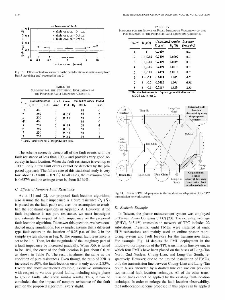
Fig. 13 illustrates the impacts of different fault resistancesunder different fault distances in line 2. An examination ofFig. 13 clearly reveals that the proposed algorithm is hardlyaffected by the magnitudes of fault resistance. Because theproposed scheme does not involve the fault resistance, it ispractically independent of fault resistance.

A total of more than 1800 simulation cases have been con-ducted with respect to various system situations and fault eventsfor the entire sample networks. The statistical evaluations of thefault-location errors and the failure cases for the proposed algo-rithm under different fault resistances are briefly summarized inTable III.


Fig. 13. Effects of faults resistances on the fault-location estimation away fromBus 3 (receiving end) occurred in line 2.

TABLE IIISUMMARY FOR THE STATISTICAL EVALUATIONS OF

THE PROPOSED FAULT-LOCATION ALGORITHM

The scheme correctly detects all of the fault events with thefault resistance of less than 100 and provides very good ac-curacy in fault location. When the fault resistance is even up to100 , only a few fault events cannot be detected by the pro-posed approach. The failure rate of this statistical study is verylow, about . In all cases, the maximum erroris 0.637% and the average error is about 0.169%.

C. Effects of Nonpure Fault Resistance

As in [1] and [2], our proposed fault-location algorithmsalso assume the fault impedance is a pure resistance (is placed on the fault path) and uses the assumption to estab-lish the constraint equations in Appendix A. However, if thefault impedance is not pure resistance, we must investigateand estimate the impact of fault impedance on the proposedfault-location algorithm. To answer this question, we have con-ducted many simulations. For example, assume that a differenttype fault occurs in the location of 0.25 p.u. of line 2 in thesample system shown in Fig. 8. The original fault resistance isset to be 1 . Then, let the magnitude of the imaginary part ofa fault impedance be increased gradually. When X/R is tunedto be 10%, the error of the fault location is just about 0.01%as shown in Table IV. The result is almost the same as thecondition of pure resistances. Even though the ratio of X/R isincreased to 50%, the fault-location error is only about 2.83%.Except the above-mentioned example, extensive simulationswith respect to various ground faults, including single-phaseto ground faults, also show similar results. Thus, it can beconcluded that the impact of nonpure resistance of the faultpath on the proposed algorithm is very slight.

TABLE IVSUMMARY FOR THE IMPACT OF FAULT IMPEDANCE VARIATIONS ON THE

PERFORMANCE OF THE PROPOSED FAULT-LOCATION ALGORITHM

Fig. 14. Status of PMU deployment in the middle-to-north portion of the TPCtransmission network system.

D. Realistic Example

In Taiwan, the phasor measurement system was employedin Taiwan Power Company (TPC) [23]. The extra-high-voltage[(EHV), 345-kV] transmission network of TPC includes 22substations. Presently, eight PMUs were installed at eightEHV substations and mainly used an online phasor moni-toring system and fault locators for the transmission lines.For example, Fig. 14 depicts the PMU deployment in themiddle-to-north portion of the TPC transmission line system, inwhich four PMUs have been placed on the buses of Lung–TanNorth, 2nd Nuclear, Chung–Liao, and Lung–Tan South, re-spectively. However, due to the limited installation of PMUs,only the transmission line between Chung–Liao and Lung–TanSouth buses encircled by a dashed line can use our previoustwo-terminal fault-location technique. All of the other trans-mission lines cannot be applied by the existing fault-locationtechnique. In order to enlarge the fault-location observability,the fault-location scheme proposed in this paper can be applied


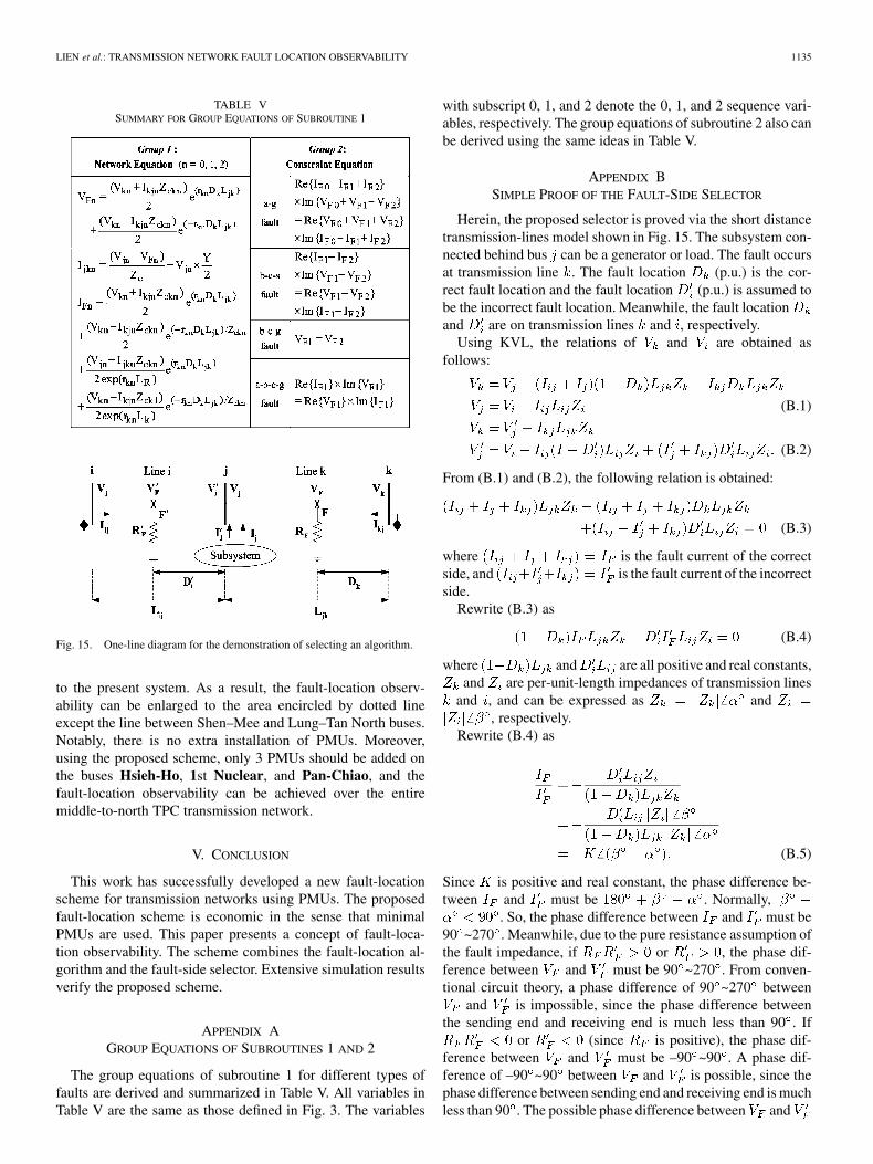
TABLE VSUMMARY FOR GROUP EQUATIONS OF SUBROUTINE 1

Fig. 15. One-line diagram for the demonstration of selecting an algorithm.

to the present system. As a result, the fault-location observ-ability can be enlarged to the area encircled by dotted lineexcept the line between Shen–Mee and Lung–Tan North buses.Notably, there is no extra installation of PMUs. Moreover,using the proposed scheme, only 3 PMUs should be added onthe buses Hsieh-Ho, 1st Nuclear, and Pan-Chiao, and thefault-location observability can be achieved over the entiremiddle-to-north TPC transmission network.

V. CONCLUSION

This work has successfully developed a new fault-locationscheme for transmission networks using PMUs. The proposedfault-location scheme is economic in the sense that minimalPMUs are used. This paper presents a concept of fault-loca-tion observability. The scheme combines the fault-location al-gorithm and the fault-side selector. Extensive simulation resultsverify the proposed scheme.

APPENDIX AGROUP EQUATIONS OF SUBROUTINES 1 AND 2

The group equations of subroutine 1 for different types offaults are derived and summarized in Table V. All variables inTable V are the same as those defined in Fig. 3. The variables

with subscript 0, 1, and 2 denote the 0, 1, and 2 sequence vari-ables, respectively. The group equations of subroutine 2 also canbe derived using the same ideas in Table V.

APPENDIX BSIMPLE PROOF OF THE FAULT-SIDE SELECTOR

Herein, the proposed selector is proved via the short distancetransmission-lines model shown in Fig. 15. The subsystem con-nected behind bus can be a generator or load. The fault occursat transmission line . The fault location (p.u.) is the cor-rect fault location and the fault location (p.u.) is assumed tobe the incorrect fault location. Meanwhile, the fault locationand are on transmission lines and , respectively.

Using KVL, the relations of and are obtained asfollows:

(B.1)

(B.2)

From (B.1) and (B.2), the following relation is obtained:

(B.3)

where is the fault current of the correctside, and is the fault current of the incorrectside.

Rewrite (B.3) as

(B.4)

where and are all positive and real constants,and are per-unit-length impedances of transmission lines

and , and can be expressed as and, respectively.

Rewrite (B.4) as

(B.5)

Since is positive and real constant, the phase difference be-tween and must be . Normally,

. So, the phase difference between and must be90 ~270 . Meanwhile, due to the pure resistance assumption ofthe fault impedance, if or , the phase dif-ference between and must be 90 ~270 . From conven-tional circuit theory, a phase difference of 90 ~270 between

and is impossible, since the phase difference betweenthe sending end and receiving end is much less than 90 . If

or (since is positive), the phase dif-ference between and must be –90 ~90 . A phase dif-ference of –90 ~90 between and is possible, since thephase difference between sending end and receiving end is muchless than 90 . The possible phase difference between and


is less than 90 . Thus, the estimated fault location with positivefault resistance is selected as the correct solution. When the faultoccurs at line , the same results can be obtained by the similarprocedures demonstrated before.

REFERENCES

[1] L. Eriksson, M. M. Saha, and G. D. Rockefeller, “An accurate fault lo-cator with compensation for apparent reactance in the fault resistanceresulting from remote-end infeed,” IEEE Trans. Power App. Syst., vol.PAS-104, no. 2, pp. 424–436, Feb. 1985.

[2] T. T. Takagi, Y. Yamakoshi, J. Baba, K. Uemura, and T. Sakaguchi, “De-velopment of a new fault locator using the one-terminal voltage andcurrent data,” IEEE Trans. Power App. Syst., vol. PAS-101, no. 8, pp.2892–2898, Aug. 1982.

[3] A. G. Phadke, “Synchronized phasor measurements in power systems,”IEEE Comput. Appl. Power, vol. 6, no. 2, pp. 10–15, Apr. 1993.

[4] R. K. Aggarwal, D. V. Doury, A. T. Johns, and A. Kalam, “A practicalapproach to accurate fault location on extra high voltage teed feeder,”IEEE Trans. Power Del., vol. 8, no. 3, pp. 874–883, Jul. 1993.

[5] D. G. Hart, D. Novosol, and E. Udren, “Application of synchronizedphasors to fault location analysis,” in Applications of Synchronized Pha-sors Conf., Precise Measurements in Power Systems Arlington, VA,Oct. 1993, vol. III-6.1-13.

[6] A. A. Girgis, D. G. Hart, and W. L. Peterson, “A new fault locationtechnique for two- and three-terminal lines,” IEEE Trans. Power Del.,vol. 7, no. 1, pp. 98–107, Jan. 1992.

[7] M. Kezunovic, J. Mrkic, and B. Perunicic, “An accurate fault locationalgorithm using synchronized sampling,” Elect. Power Syst. Res., vol.29, no. 3, pp. 161–169, May 1994.

[8] A. O. Ibe and B. J. Cory, “A traveling wave based fault locator for two-and three-terminal networks,” IEEE Trans. Power Syst., vol. PWRD-1,no. 1, pp. 283–288, Jan. 1986.

[9] J.-A. Jiang, J.-Z. Yang, Y.-H. Lin, C.-W. Liu, and J.-C. Ma, “An adaptivePMU based fault detection/location technique for transmission lines-partI: Theory and algorithms,” IEEE Trans. Power Del., vol. 15, no. 2, pp.486–493, Apr. 2000.

[10] J.-A. Jiang, Y.-H. Lin, J.-Z. Yang, T.-M. Too, and C.-W. Liu, “Anadaptive PMU based fault detection/location technique for transmissionlines-part II: PMU implementation and performance evaluation,” IEEETrans. Power Del., vol. 15, no. 4, pp. 1136–1146, Oct. 2000.

[11] C.-S. Chen, C.-W. Liu, and J.-A. Jiang, “A new adaptive PMU based pro-tection scheme for transposed/untransposed parallel transmission lines,”IEEE Trans. Power Del., vol. 17, no. 2, pp. 395–404, Apr. 2002.

[12] C.-S. Yu, C.-W. Liu, S.-L. Yu, and J.-A. Jiang, “A new PMU based faultlocation algorithm for series compensated lines,” IEEE Trans. PowerDel., vol. 17, no. 1, pp. 33–46, Jan. 2002.

[13] Y.-H. Lin, C.-W. Liu, and C.-S. Yu, “A new fault locator for three-ter-minal transmission line-using two-terminal synchronized voltage andcurrent phasors,” IEEE Trans. Power Del., vol. 17, no. 2, pp. 452–459,Apr. 2002.

[14] T. L. Baldwin, L. Mili, M. B. Boisen Jr, and R. Adapa, “Power systemobservability with minimal phasor measurement placement,” IEEETrans. Power Syst., vol. 8, no. 2, pp. 707–715, May 1993.

[15] C. A. Gross, Power System Analysis. New York: Wiley, 1986.[16] J. R. Rice, Numerical Methods, Software, and Analysis. San Diego,

CA: Academic, 1993.[17] C.-S Yu, C.-W Liu, and Y.-H Lin, “A fault location algorithm for trans-

mission lines with tapped leg—PMU based approach,” in Proc. PowerEng. Soc. Summer Meeting, vol. 2, Jul. 2001, pp. 915–920.

[18] D. Novosel, D. G. Hart, E. Udren, and M. M. Saha, “Fault location usingdigital relay data,” IEEE Comput. Appl. Power, vol. 8, no. 3, pp. 45–50,Jul. 1995.

[19] H. Dommel, “Electromagnetic Transient Program,” BPA, Portland, OR,1986.

[20] G. Benmouyal, “Removal of DC-Offset in current waveforms usingdigital mimic filtering,” IEEE Trans. Power Del., vol. 10, no. 2, pp.621–630, Apr. 1995.

[21] W. D. Stevenson Jr, Elements of Power System Analysis. New York:McGraw-Hill, 1982.

[22] W. A. Elmore, Protective Relaying Theory and Applications. CoralSprings, FL: ABB, 1994.

[23] C.-W Liu, “Phasor measurement applications in Taiwan,” in Proc. IEEETransmission and Distribution Conf. Exhibit., vol. 1, Yokohama, Japan,Oct. 2002, pp. 490–493.

Kai-Ping Lien (S’01) was born in Tainan, Taiwan, R.O.C., in 1970. He receivedthe B.S. degree in electrical engineering from National Sun Yat-Sen University,Kaoshuing, in 1992. He is currently pursuing the Ph.D. degree in electrical en-gineering at National Taiwan University, Taipei.

Chih-Wen Liu (S’93–M’96–SM’02) was born in Taiwan, R.O.C., in 1964. Hereceived the B.S. degree in electrical engineering from National Taiwan Univer-sity (NTU), Taipei, Taiwan, in 1987, and the M.S. and Ph.D. degrees in electricalengineering from Cornell University, Ithaca, NY, in 1992 and 1994, respectively.

Currently, he is with NTU, where he is a Professor of electrical engineering.His main research interests include the application of computer technology topower system monitoring, protection, and control. His research interests includemotor control and power electronics.

Chi-Shan Yu (S’99–M’01) was born in Taipei, Taiwan, R.O.C., in 1966. Hereceived the B.S. and M.S. degrees in electrical engineering from National TsingHua University, Hsinchu, in 1988 and 1990, respectively, and the Ph.D. degreein electrical engineering from National Taiwan University, Taipei, in 2001.

Currently, he is Associate Professor of Electrical Engineering with the Na-tional Defense University, Chung-Cheng Institute of Technology. His researchareas are computer relaying, power system transient stability controller design,and power electronics.

Joe-Air Jiang (M’01) was born in Tainei, Taiwan, R.O.C., in 1963. He receivedthe M.S. and Ph.D. degrees in electrical engineering from National Taiwan Uni-versity, Taipei, in 1990 and 1999, respectively.

Currently, he is an Associate Professor of bio-industrial mechatronics engi-neering at National Taiwan University. His research interests are in computerrelaying, mechatronics, and bioeffects of the electromagnetic wave.

transmission network fault location observability with minimal pmu placement

Documents