On the Impact of PMU Placement on Observability and

Cross-Validation

Technical Report UM-CS-2012-001Daniel Gyllstrom, Elisha Rosensweig, and Jim Kurose

Department of Computer Science. University of Massachusetts Amherst USA{dpg, elisha, kurose}@cs.umass.edu

ABSTRACTSignificant investments have been made into deploying pha-sor measurement units (PMUs) on electric power grids world-wide. PMUs allow the state of the power system – thevoltage phasor of system buses and current phasors of allincident transmission lines – to be directly measured. Insome cases, it is also possible to infer the voltage and cur-rent phasors at neighboring buses and lines. Because PMUsare expensive, it is typically not possible to deploy enoughPMUs to observe all phasors in a grid network [3, 6].

In this paper, we prove the NP-Completeness of four prob-lems relating to PMU placements at a subset of system busesto achieve different goals: FullObserve, MaxObserve,FullObserve-XV, and MaxObserve-XV. FullObserve

considers the minimum number of PMUs needed to observeall nodes, while MaxObserve considers the maximum num-ber of buses that can be observed with a given number ofPMUs. While the first of these two has been considered inthe past, our formulation here generalizes the systems beingconsidered. Next, FullObserve-XV and MaxObserve-

XV consider these two problems under the constraints thatPMUs must be placed“close” to each other so their measure-ments can be cross-validated. FullObserve-XV considersobserving the entire network, while MaxObserve-XV con-siders maximizing the number of observed buses under thisnew constraint.

Motivated by their high complexity, for each problem weinvestigate the performance of a suitable greedy approxima-tion algorithm for PMU placement. Through simulations,we compare the performance of these algorithms with theoptimal placement of PMUs over several IEEE bus systemsas well as over synthetic graphs. In our simulations thesealgorithms yield results that are close to optimal - for allfour placement problems, the greedy algorithms yield, onaverage, a PMU placement that is within 97% of optimal.

1. INTRODUCTIONSignificant investments have been made to deploy phasor

Permission to make digital or hard copies of all or part of this work forpersonal or classroom use is granted without fee provided that copies arenot made or distributed for profit or commercial advantage and that copiesbear this notice and the full citation on the first page. To copy otherwise, torepublish, to post on servers or to redistribute to lists, requires prior specificpermission and/or a fee.Copyright 20XX ACM X-XXXXX-XX-X/XX/XX ...$10.00.

measurement units (PMUs) on electric power grids world-wide. A new generation of PMUs provides synchronizedvoltage and current measurements at a sampling rate or-ders of magnitude higher than the status quo: 10 to 60samples per second rather than one sample every 1 to 4seconds. Consequently, PMUs have the potential to enablean entirely new set of applications for the power grid: pro-tection and control during abnormal conditions, real-timedistributed control, postmortem analysis of system faultsusing time synchronized data, advanced state estimators forsystem monitoring, and the reliable integration of renewableenergy resources [1].

An electric power system consists of a set of buses – anelectric substation, power generation center, or aggregationof loads – and transmission lines connecting those buses.The state of a power system is defined by the voltage phasor– the magnitude and phase angle – of all system buses andthe current phasor of all transmission lines. PMUs placedon buses provide real-time measurements of these systemvariables. However, because PMUs are expensive, they can-not be deployed on all system buses [3][6]. Fortunately, thevoltage phasor at a system bus can, at times, be determined(termed observed in this paper) even when a PMU is notplaced at that bus, by applying Ohm’s and Kirchhoff’s lawson the measurements taken by a PMU placed at some nearbysystem bus [3][4]. Specifically, with correct placement ofenough PMUs at a subset of system buses, the entire sys-tem state can be determined.

In this work, we study two sets of PMU placement prob-lems. The first problem set consists of FullObserve andMaxObserve, and considers maximizing the observabilityof the network via PMU placement. FullObserve consid-ers the minimum number of PMUs needed to observe allsystem buses, while MaxObserve considers the maximumnumber of buses that can be observed with a given number ofPMUs. A bus is said to be observed if there is a PMU placedat it or if its voltage phasor can be estimated using Ohm’sor Kirchhoff’s Law. Although FullObserve is well stud-ied [3, 4, 9, 11, 14], existing work considers only networksconsisting solely of zero-injection buses, while we general-ize the problem formulation to include mixtures of zero andnon-zero-injection buses. Additionally, our approach for an-alyzing FullObserve provides the foundation with whichto present the other three new (but related) PMU placementproblems.

The second set of placement problems considers PMUplacements that support PMU error detection. PMU mea-surement errors have been recorded in actual systems [13].

One method of detecting these errors is to deploy PMUs“near” each other, thus enabling them to cross-validate each-other’s measurements. FullObserve-XV aims to minimizethe number of PMUs needed to observe all buses while insur-ing PMU cross-validation, and MaxObserve-XV computesthe maximum number of observed buses for a given numberof PMUs, while insuring PMU cross-validation.

We make the following contributions in this paper:

• We formulate two PMU placement problems, which(broadly) aim at maximizing observed buses while min-imizing the number of PMUs used. Our formulationextends previously studied systems by considering bothzero and non-zero-injection buses.

• We formally define graph-theoretic rules for PMU cross-validation. Using these rules, we formulate two addi-tional PMU placement problems that seek to maxi-mize the observed buses while minimizing the numberof PMUs used under the condition that the PMUs arecross-validated.

• We prove that all four PMU placement problems areNP-Complete. This represents our most importantcontribution.

• Given the proven complexity of these problems, weevaluate heuristic approaches for solving these prob-lems. For each problem we describe a greedy algo-rithm, and prove that each greedy algorithm has poly-nomial running time.

• Using simulations, we evaluate the performance of ourgreedy approximation algorithms over synthetic andactual IEEE bus systems. We find that the greedy al-gorithms yield a PMU placement that is, on average,within 97% optimal. Additionally, we find that thethe cross-validation constraints have limited effects onobservability: on average our greedy algorithm thatplaces PMUs according to the cross-validation rulesobserves only 5.7% fewer nodes than the same algo-rithm that does not consider cross-validation.

The rest of this paper is organized as follows. In Section 2we introduce our modeling assumptions, notation, and ob-servability and cross-validation rules. In Section 3 we formu-late and prove the complexity of our four PMU placementproblems. Section 4 presents the approximation algorithmsfor each problem, and Section 5 considers the results of oursimulation-based evaluation. We conclude this paper with areview of related work (Section 6) and concluding remarks(Section 7).

2. PRELIMINARIESIn this section we introduce notation and underlying as-

sumptions (Section 2.1), and define our observability (Sec-tion 2.2) and cross-validation (Section 2.3) rules.

2.1 Assumptions, Notation, and TerminologyConsistent with the conventions in [3, 4, 5, 11, 14, 15],

we make the following assumptions about PMU placementsand buses:

1. A PMU can only be placed on a bus.

ba

c hi

fd

g

j

e

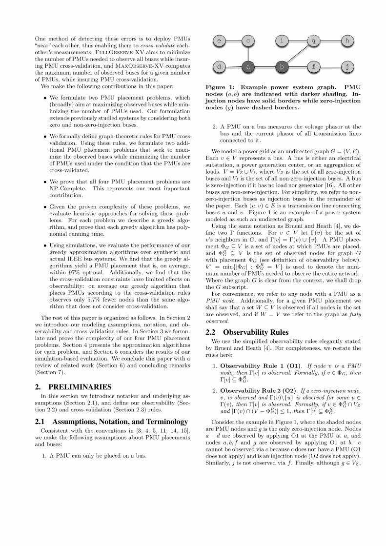
Figure 1: Example power system graph. PMU

nodes (a, b) are indicated with darker shading. In-

jection nodes have solid borders while zero-injection

nodes (g) have dashed borders.

2. A PMU on a bus measures the voltage phasor at thebus and the current phasor of all transmission linesconnected to it.

We model a power grid as an undirected graph G = (V, E).Each v ∈ V represents a bus. A bus is either an electricalsubstation, a power generation center, or an aggregation ofloads. V = VZ ∪ VI , where VZ is the set of all zero-injectionbuses and VI is the set of all non-zero-injection buses. A busis zero-injection if it has no load nor generator [16]. All otherbuses are non-zero-injection. For simplicity, we refer to non-zero-injection buses as injection buses in the remainder ofthe paper. Each (u, v) ∈ E is a transmission line connectingbuses u and v. Figure 1 is an example of a power systemmodeled as such an undirected graph.

Using the same notation as Brueni and Heath [4], we de-fine two Γ functions. For v ∈ V let Γ(v) be the set ofv’s neighbors in G, and Γ[v] = Γ(v) ∪ {v}. A PMU place-ment ΦG ⊆ V is a set of nodes at which PMUs are placed,and ΦR

G ⊆ V is the set of observed nodes for graph Gwith placement ΦG (see definition of observability below).k∗ = min{|ΦG| : ΦR

G = V } is used to denote the mini-mum number of PMUs needed to observe the entire network.Where the graph G is clear from the context, we shall dropthe G subscript.

For convenience, we refer to any node with a PMU as aPMU node. Additionally, for a given PMU placement weshall say that a set W ⊆ V is observed if all nodes in the setare observed, and if W = V we refer to the graph as fully

observed.

2.2 Observability RulesWe use the simplified observability rules elegantly stated

by Brueni and Heath [4]. For completeness, we restate therules here:

1. Observability Rule 1 (O1). If node v is a PMU

node, then Γ[v] is observed. Formally, if v ∈ ΦG, then

Γ[v] ⊆ ΦR

G.

2. Observability Rule 2 (O2). If a zero-injection node,

v, is observed and Γ(v)\{u} is observed for some u ∈Γ(v), then Γ[v] is observed. Formally, if v ∈ ΦR

G ∩ VZ

and |Γ(v) ∩ (V − ΦR

G)| ≤ 1, then Γ[v] ⊆ ΦR

G.

Consider the example in Figure 1, where the shaded nodesare PMU nodes and g is the only zero-injection node. Nodesa − d are observed by applying O1 at the PMU at a, andnodes a, b, f and g are observed by applying O1 at b. ecannot be observed via c because c does not have a PMU (O1does not apply) and is an injection node (O2 does not apply).Similarly, j is not observed via f . Finally, although g ∈ VZ ,

O2 cannot be applied at g because g has two unobservedneighbors i, h, so they remain unobserved.

Since O2 only applies with zero-injection nodes, morenodes might be observed when nodes are zero-injection. Forexample, consider the case where c and f are zero-injection

nodes. a−d, g and f are still observed as before, as O1 makesnot conditions on the node type. Additionally, since nowc, f ∈ VZ and each has a single unobserved neighbor, we canapply O2 at each of them to observe e, j, respectively. Weevaluate the effect of increasing the number of zero-injectionnodes on observability in our simulations (Section 5.2).

2.3 Cross-Validation RulesFrom Vanfretti et al. [13], PMU measurements can be

cross-validated when: (1) a voltage phasor of a non-PMUbus can be computed by PMU data from two different busesor (2) the current phasor of a transmission line can be com-puted from PMU data from two different buses. 1 Althoughit is the PMU data that is actually being cross-validated,for convenience, we say a PMU is cross-validated. A PMUis cross-validated if one of the rules below is satisfied [13]:

1. Cross-Validation Rule 1 (XV1). If two PMU nodes

are adjacent, then the PMUs cross-validate each other.

Formally, if u, v ∈ ΦG, u ∈ Γ(v), then the PMUs at uand v are cross-validated.

2. Cross-Validation Rule 2 (XV2). If two PMU nodes

have a common neighbor, then the PMUs cross-validate

each other. Formally, if u, v ∈ ΦG, u �= v and Γ(u) ∩Γ(v) �= ∅, then the PMUs at u and v are cross-validated.

In short, the cross-validation rules require that the PMU is

within two hops of another PMU. For example, in Figure 1,the PMUs at a and b cross-validate each other by XV1.

XV1 derives from the fact that both PMUs are measur-ing the current phasor of the transmission line connectingthe two PMU nodes. XV2 is more subtle. Using the nota-tion specified in XV2, when computing the voltage phasorof an element in Γ(u) ∩ Γ(v) the voltage equations includevariables to account for measurement error (e.g., angle bias)[12]. When the PMUs are two hops from each other, thereare more equations than unknowns, allowing for measure-ment error detection. Otherwise, the number of unknownvariables exceeds the number of equations, which eliminatesthe possibility of detecting measurement errors [12].

3. PROBLEM FORMULATIONS AND NP-COMPLETENESS PROOFS

In this section we define four PMU placement problemsand prove the NP-Completeness of each. We begin witha general overview of NP-Completeness, as well as a high-level description of our proof strategy in this paper (Section3.1). In the remainder of Section 3 we present and provethe NP-Completeness of four PMU placement problems, inthe following order: FullObserve (Section 3.2), MaxOb-

serve (Section 3.3), FullObserve-XV (Section 3.4), andMaxObserve-XV (Section 3.5).

In all four problems defined in this paper, we are onlyconcerned with computing the voltage phasors of each bus(i.e., observing the buses). Using the values of the voltage1Vanfretti et al. [13] use the term “redundancy” instead of cross-validation.

phasors, Ohm’s Law can be easily applied to compute thecurrent phasors of each transmission line. Also, we con-sider networks with both injection and zero-injection buses.For similar proofs for purely zero-injection systems, see ourTechnical Report [8].

3.1 NP-Completeness Overview and Proof Strat-egy

Before proving that our PMU placement problems are NP-Complete (abbreviated NPC), we provide some backgroundon NP-Completeness. NPC problems are the hardest prob-lems in complexity class NP. It is generally assumed thatsolving NPC problems is hard, meaning that any algorithmthat solves an NPC problem has exponential running timeas function of the input size. It is important to clarify thatdespite being NPC, a specific problem instance might be ef-ficiently solvable. This is either due to the special structureof the specific instance or because the input size is small,yielding a small exponent. For example, in Section 5 weare able to solve FullObserve for small IEEE bus topolo-gies due to their small size. Thus, by establishing that ourPMU placement problems are NPC, we claim that there ex-

ist bus topologies for which these problems are difficult tosolve (i.e., no known polynomial-time algorithm exists tosolve those case).

To prove our problems are NPC, we follow the standardthree-step reduction procedure. For a decision problem Π,we first show Π ∈ NP. Second, we select a known NPCproblem, denoted Π�, and construct a polynomial-time trans-formation, f , that maps any instance of Π� to an instance ofΠ. Finally, we must ensure that for this f , x ∈ Π� ⇔ f(x) ∈Π [7].

Next, we outline the proof strategy we use throughoutthe paper. In Sections 3.2 through Section 3.5 we use slightvariations of the approach presented by Brueni and Heathin [4] to prove the problems we consider here are NPC. Ingeneral we found their scheme to be elegantly extensible forproving many properties of PMU placements.

In [4], the authors prove NP-Completeness by reductionfrom planar 3-SAT (P3SAT). A 3-SAT formula, φ, is aboolean formula in conjunctive normal form (CNF) suchthat each clause contains at most 3 literals. For any 3-SAT formula φ with the sets of variables {v1, v2, . . . , vr} andclauses {c1, c2, . . . , cs}, G(φ) is the bipartite graph G(φ) =(V (φ), E(φ)) defined as follows:

V (φ) = {vi | 1 ≤ i ≤ r} ∪ {cj | 1 ≤ j ≤ s}E(φ) = {(vi, cj) | vi ∈ cj or vi ∈ cj}.

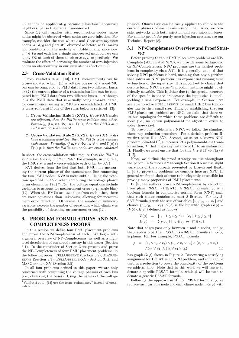
Note that edges pass only between v and c nodes, and sothe graph is bipartite. P3SAT is a 3-SAT formula s.t. G(φ)is planar [10]. For example, P3SAT formula

ϕ = (v1 ∨ v2 ∨ v3) ∧ (v1 ∨ v4 ∨ v5) ∧ (v2 ∨ v3 ∨ v5)

∧(v3 ∨ v4) ∧ (v3 ∨ v4 ∨ v5) (1)

has graph G(ϕ) shown in Figure 2. Discovering a satisfyingassignment for P3SAT is an NPC problem, and so it can beused in a reduction to prove the complexity of the problemswe address here. Note that in this work we will use ϕ todenote a specific P3SAT formula, while φ will be used todenote a generic P3SAT formula.

Following the approach in [4], for P3SAT formula, φ, wereplace each variable node and each clause node in G(φ) with

v3

v2

v4

v1

v5

c1

c4c2

c5 c3

Figure 2: G(ϕ) = (V (ϕ), E(ϕ)) formed from ϕ in Equa-

tion (1)

a specially constructed set of nodes, termed a gadget. In thiswork, all variable gadgets will have the same structure, andall clause gadgets have the same structure (that is differentfrom the variable gadget structure), and we denote the re-sulting graph as H(φ). In H(φ), each variable gadget has asubset of nodes that semantically represent assigning “True”to that variable, and a subset of nodes that represent assign-ing it “False”. When a PMU is placed at one of these nodes,this is interpreted as assigning a truth value to the P3SAT

variable corresponding with that gadget. Thus, we use thePMU placement to determine a consistent truth value foreach P3SAT variable. Also, clause gadgets are connected tovariable gadgets at either “True” or “False” (but never both)nodes, in such a way that the clause is satisfied if and onlyif at least one of those nodes has a PMU.

We also note that while we assume G(φ) is planar, wemake no such claim regarding H(φ), though in practice allgraphs used in our proofs are indeed planar. The proof ofNPC rests on the fact that solving the underlying φ formulais NPC.

In what follows, for a given PMU placement problem Π,we prove Π is NPC by showing that a PMU placement inH(φ), Φ, can be interpreted semantically as describing asatisfying assignment for φ iff Φ ∈ Π. Since P3SAT is NPC,this proves Π is NPC as well.

3.2 The FullObserve ProblemThe FullObserve problem was previously discussed in

the literature (e.g., the PMUP problem in [4], and the PDSproblem in [9]) for purely zero-injection bus systems. Herewe consider networks with mixtures of injection and zero-injection buses, and modify the NPC proof for PMUP in [4]to handle this mixture.

FullObserve Optimization Problem:

• Input: Graph G = (V, E) where V = VZ ∪ VI and

VZ �= ∅. 2

• Output: A placement of PMUs, ΦG, such that ΦR

G = Vand ΦG is minimal.

2We include the condition that VZ �= ∅ because otherwiseFullObserve reduces to Vertex-Cover, making the NP-Completeness proof trivial.

FiTi

Ii

Zi

(a) Variable gadget Vi used in Theorem3.1 and Theorem 3.4. The dashed edgesare connections to clause gadgets. Zi isa zero-injection node and all other nodesare injection nodes.

ajbj

(b) Clausegadget Cj

used in The-orem 3.4.The dashededges areconnectionsto variablegadgets. aj

and bj areboth injectionnodes.

Figure 3: Gadgets used in Theorem 3.1 and Theo-

rem 3.4.

FullObserve Decision Problem:

• Instance: Graph G = (V, E) where V = VZ ∪VI , VZ �=∅, k PMUs such that k ≥ 1.

• Question: Is there a ΦG such that |ΦG| ≤ k and ΦR

G =V ?

Theorem 3.1. FullObserve is NP-Complete.

Proof Idea: We introduce a problem-specific variablegadget. We show that in order to observe all nodes, PMUsmust be placed on variable gadgets, specifically on nodesthat semantically correspond to True and False values thatsatisfy the corresponding P3SAT formula.

For our first problem, we use a single node as a clausegadget denoted aj , and the subgraph shown in Figure 3(a)as the variable gadget. Note that in the variable gadget,all the nodes are injection nodes except for Zi. For thissubgraph, we state the following simple lemma:

Lemma 3.2. Consider the gadget shown in Figure 3(a),

possibly with additional edges connected to Ti and/or Fi.

Then (a) nodes Ii, Zi are not observed if there is no PMU on

the gadget, and (b) all the nodes in the gadget are observed

with a single PMU iff the PMU is placed on either Ti or Fi.

Proof. (a) If there is no PMU on the gadget, O1 cannotbe applied at any of the nodes, and so we must resort toO2. We assume no edges connected to Ii, Zi from outsidethe gadget, and since Ti, Fi ∈ VI , we cannot apply O2 atthem, which concludes our proof.

(b) In one direction, if we have a PMU placed at Ti, fromO1 we can observe Zi, Ii. Since Zi is zero-injection andone neighbor, Ti has been observed, from O2 at Zi we canobserve Fi. The same holds for placing a PMU at Fi, dueto symmetry.

In the other direction, by placing a PMU at Ii (Zi) weobserve Ti and Fi via O1. However, since Fi, Ti /∈ VZ , O2cannot be applied at either of them, so Zi (Ii) will not beobserved.

Proof of Theorem 3.1. We start by arguing that Ful-

lObserve ∈ NP. First, nondeterministically select k nodesin which to place PMUs. Using the rules specified in Section2.2, determining the number of observed nodes can be donein linear time.

To show FullObserve is NP-hard, we reduce from P3SAT.Let φ be an arbitrary P3SAT formula with variables {v1, v2, . . . , vr}and the set of clauses {c1, c2, . . . , cs}, and G(φ) the corre-sponding planar graph. We use G(φ) to construct a newgraph H0(φ) = (V0(φ), E0(φ)) by replacing each variablenode in G(φ) with the variable gadget shown in Figure 3(a).The clause nodes consist of a single node (i.e., are the sameas in G(φ)). We denote the node corresponding to cj as aj .All clause nodes are injection nodes. In the remainder ofthis proof we let H := H0(φ). In total, VZ contains all Zi

nodes for 1 ≤ i ≤ r, and all other nodes are in VI . Theedges connecting clause nodes with variable gadgets expresswhich variables are in each clause: for each clause node aj ,(Ti, aj) ∈ E0(φ) ⇔ vi ∈ cj , and (Fi, aj) ∈ E0(φ) ⇔ vi ∈ cj .As a result, the following observation holds:

Observation 3.3. For a given truth assignment and a cor-

responding PMU placement, a clause cj is satisfied iff aj is

attached to a node in a variable gadget with a PMU.

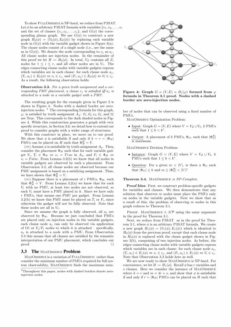
The resulting graph for the example given in Figure 2 isshown in Figure 4. Nodes with a dashed border are zero-injection nodes. 3 The corresponding formula for this graph,ϕ, is satisfied by truth assignment Aϕ: v1, v2, v3, v4, and v5

are True. This corresponds to the dark shaded nodes in Fig-ure 4. While this construction generates a graph with veryspecific structure, in Section 3.6, we detail how to extend ourproof to consider graphs with a wider range of structures.

With this construct in place, we move on to our proof.We show that φ is satisfiable if and only if k = r = |ΦH |PMUs can be placed on H such that ΦR

H = V .(⇒) Assume φ is satisfiable by truth assignment Aφ. Then,

consider the placement ΦH such that for each variable gad-get Vi, Ti ∈ ΦH ⇔ vi = True in Aφ, and Fi ∈ ΦH ⇔vi = False. From Lemma 3.2(b) we know that all nodes invariable gadgets are observed by such a placement. FromObservation 3.3, all clause nodes are observed because ourPMU assignment is based on a satisfying assignment. Thus,we have shown that ΦR

H = V .(⇐) Suppose there is a placement of r PMUs, ΦH , such

that ΦR

H = V . From Lemma 3.2(a) we know that for eachVi with no PMU, at least two nodes are not observed, soeach Vi must have a PMU placed in it. Since we have onlyr PMUs, that means one PMU per gadget. From Lemma3.2(b) we know this PMU must be placed on Ti or Fi, sinceotherwise the gadget will not be fully observed. Note thatthese nodes are all in VI .

Since we assume the graph is fully observed, all aj areobserved by ΦH . Because we just concluded that PMUsare placed only on injection nodes in the variable gadgets,each clause node aj can only be observed via applicationof O1 at Ti/Fi nodes to which it is attached – specifically,aj is attached to a node with a PMU. From Observation3.3 this means that all clauses are satisfied by the semanticinterpretation of our PMU placement, which concludes ourproof.

3.3 The MaxObserve ProblemMaxObserve is a variation of FullObserve: rather than

consider the minimum number of PMUs required for full sys-tem observability, MaxObserve finds the maximum num-3Throughout this paper, nodes with dashed borders denote zero-injection nodes.

V1

C1

C4C2

C5 C3

V2

V3

V4

V5

Figure 4: Graph G = (V, E) = H1(ϕ) formed from ϕformula in Theorem 3.1 proof. Nodes with a dashed

border are zero-injection nodes.

ber of nodes that can be observed using a fixed number ofPMUs.

MaxObserve Optimization Problem:

• Input: Graph G = (V, E) where V = VZ ∪VI , k PMUssuch that 1 ≤ k < k∗.

• Output: A placement of k PMUs, ΦG, such that |ΦR

G|is maximum.

MaxObserve Decision Problem:

• Instance: Graph G = (V, E) where V = VZ ∪ VI , kPMUs such that 1 ≤ k < k∗.

• Question: For a given m < |V |, is there a ΦG such

that |ΦG| ≤ k and m ≤ |ΦR

G| < |V |?

Theorem 3.4. MaxObserve is NP-Complete.

Proof Idea: First, we construct problem-specific gadgetsfor variables and clauses. We then demonstrate that anysolution that observes m nodes must place the PMUs onlyon nodes in the variable gadgets. Next we show that asa result of this, the problem of observing m nodes in thisgraph reduces to Theorem 3.1.

Proof. MaxObserve ∈ NP using the same argumentin the proof for Theorem 3.1.

Next, we reduce from P3SAT as in the proof for Theo-rem 3.1, where φ is an arbitrary P3SAT formula. We createa new graph H1(φ) = (V1(φ), E1(φ)) which is identical toH0(φ) from the previous proof, except that each clause nodein H0(φ) is replaced with the clause gadget shown in Fig-ure 3(b), comprising of two injection nodes. As before, theedges connecting clause nodes with variable gadgets expresswhich variables are in each clause: for each clause node aj ,(Ti, aj) ∈ E1(φ) ⇔ vi ∈ cj , and (Fi, aj) ∈ E1(φ) ⇔ vi ∈ cj .Note that Observation 3.3 holds here as well.

We are now ready to show MaxObserve is NP-hard. Forconvenience, we let H := H1(φ). Recall φ has r variables ands clauses. Here we consider the instance of MaxObserve

where k = r and m = 4r + s, and show that φ is satisfiableif and only if r = |ΦH | PMUs can be placed on H such that

m ≤ |ΦR

H | < |V |. In Section 3.6 we discuss how to extend

this proof for any larger value of m and different |VZ ||VI | ratios.

(⇒) Assume φ is satisfiable by truth assignment Aφ. Then,consider the placement ΦH such that for each variable gad-get Vi, Ti ∈ ΦH ⇔ vi = True in Aφ, and Fi ∈ ΦH ⇔ vi =False. In the proof for Theorem 3.1 we demonstrated sucha placement will observe all nodes in H0(φ) ⊂ H1(φ), andusing the same argument it can easily be checked that thesenodes are still observed in H1(φ). Each bj node remains un-observed because each aj ∈ VI and consequently O2 cannotbe applied at aj . Since |H0(φ)| = 4r + s = m, we haveobserved the required nodes.

(⇐) We begin by proving that any solution that observesm nodes must place the PMUs only on nodes in the variablegadgets. By construction, each PMU is either on a clausegadget or a variable gadget, but not both. Let 0 ≤ t ≤ rbe the number of PMUs on clause gadgets, we wish to showthat for the given placement t = 0. First, note that at least

max(s− t, 0) clause gadgets are without PMUs, and that foreach such clause (by construction) at least one node (bi) isnot observed. Next, from Lemma 3.2(a) we know that foreach variable gadget without a PMU, at least two nodes arenot observed.

Denote the unobserved nodes for a given PMU placementas Φ−

H. Thus, we get |Φ−

H| ≥ 2t + max((s− t), 0). However,

since m nodes are observed and |V |−m ≤ s, we get |Φ−H| ≤ s,

so we know s ≥ 2t + max((s− t), 0). We consider two cases:

• s ≥ t: then we get s ≥ t + s ⇒ t = 0.

• s < t: then we get s ≥ 2t, and since we assume here0 ≤ s < t this leads to a contradiction and so this casecannot occur.

Thus, the r PMUs must be on nodes in variable gadgets.Note that the variable gadgets in H1(φ) have the same struc-ture as in H0(φ). We return to this point shortly.

Earlier we noted that for each clause gadget without aPMU, the corresponding bj node is unobserved, which comesto s nodes. To observe m = 4r + s nodes, we will need toobserve all the remaining nodes. Thus, we have reduced theproblem to that of observing all of H0(φ) ⊂ H1(φ). Ourproof for Theorem 3.1 demonstrated this can only be doneby placing PMUs at nodes corresponding to a satisfying as-signment of φ, and so our proof is complete.

3.4 The FullObserve-XV ProblemFullObserve-XV Optimization Problem:

• Input: Graph G = (V, E) where V = VZ ∪ VI .

• Output: A placement of PMUs, ΦG, such that ΦR

G =V , and ΦG is minimal under the condition that eachv ∈ ΦG is cross-validated according to the rules speci-fied in Section 3.4.

FullObserve-XV Decision Problem:

• Instance: Graph G = (V, E) where V = VZ ∪ VI , kPMUs such that k ≥ 1.

• Question: Is there a ΦG such that |ΦG| ≤ k and

ΦR

G = V under the condition that each v ∈ ΦG iscross-validated?

FiTiIi

Zi

FiTiIi

Zi

t

t

t

t

b b

b

b

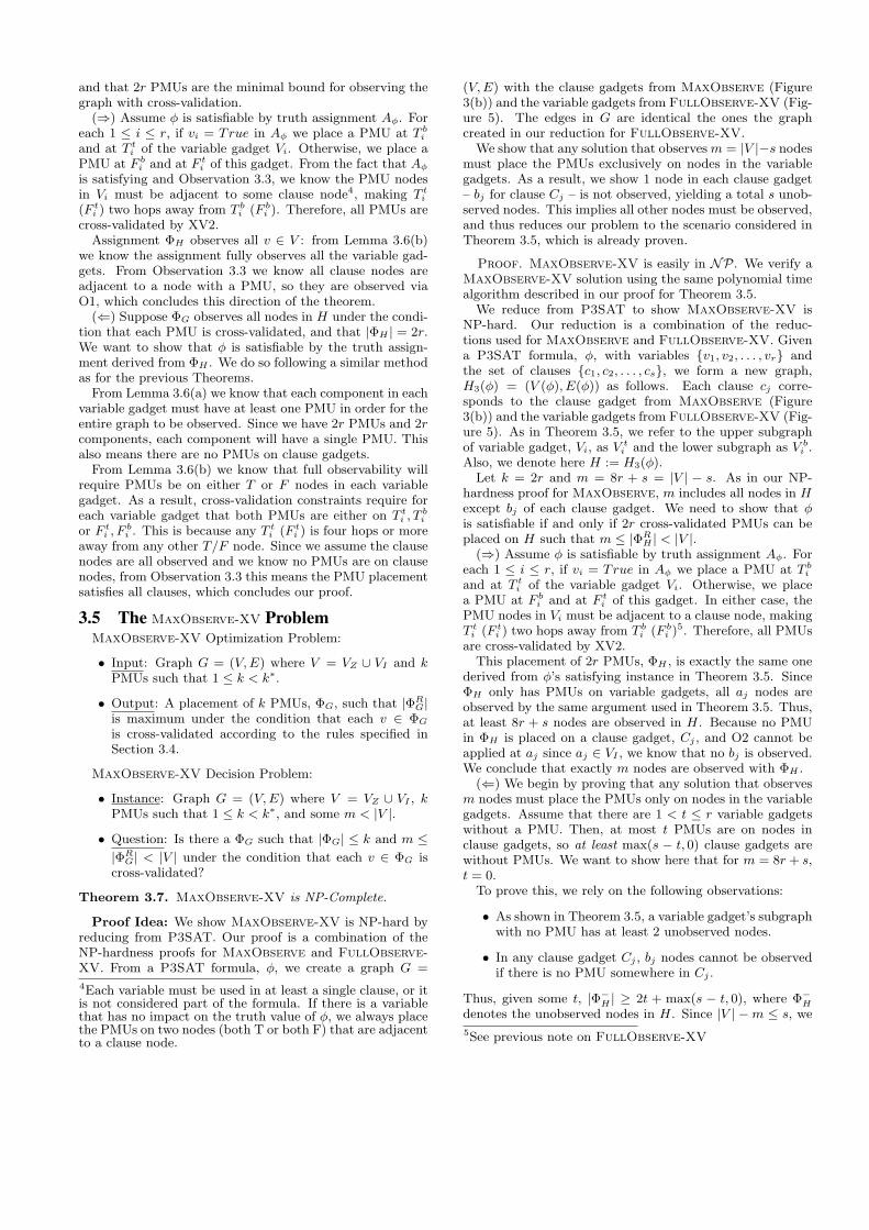
Figure 5: Variable gadget used in Theorem 3.5

proof. The gadget has two disconnected subgraphs,

where the superscript, t, denotes nodes in the up-

per subgraph and superscript, b, indexes nodes in

the lower subgraph. The dashed edges are connec-

tions to clause gadgets.

Theorem 3.5. FullObserve-XV is NP-Complete.

Proof Idea: We show FullObserve-XV is NP-hard byreducing from P3SAT. We create a single-node gadget forclauses (as for FullObserve) and the gadget shown in Fig-ure 5 for each variable. Each variable gadget here comprisesof two disconnected components, and there are two Ti andtwo Fi nodes, one in each component. First, we show thateach variable gadget must have 2 PMUs for the entire graphto be observed, one PMU for each subgraph. Then, we showthat cross-validation constraints force PMUs to be placed onboth T nodes or both F nodes. Finally, we show how to usethe PMU placement to derive a satisfying P3SAT truth as-signment.

Lemma 3.6. Consider the gadget shown in Figure 5, pos-

sibly with additional nodes attached to Ti and/or Fi nodes.

(a) nodes It

i , Zt

i are not observed if there is no PMU on V t

i ,

and (b) all the nodes in V t

i are observed with a single PMU

iff the PMU is placed on either T t

i or F t

i . Due to symmetry,

the same holds when considering V b

i .

Proof. The proof is straightforward from the proof ofLemma 3.2, since both V t

i and V b

i are identical to the gadgetfrom Figure 3(a), which Lemma 3.2 refers to.

Proof of Theorem 3.5. First, we argue that FullObserve-

XV ∈ NP. Given a FullObserve-XV solution, we use thepolynomial time algorithm described in our proof for The-orem 3.1 to determine if all nodes are observed. Then, foreach PMU node we run a breadth-first search, stopping atdepth 2, to check that the cross-validation rules are satisfied.

To show FullObserve-XV is NP-hard, we reduce fromP3SAT. Our reduction is similar to the one used in Theorem3.1. We start with the same P3SAT formula φ with variables{v1, v2, . . . , vr} and the set of clauses {c1, c2, . . . , cs}.

For this problem, we construct H2(φ) in the followingmanner. We use the single-node clause gadgets as in H0(φ),and as before, the edges connecting clause nodes with vari-able gadgets shown in Figure 5 express which variables arein each clause: for each clause node aj , (T t

i , aj), (Tb

i , aj) ∈E1(φ) ⇔ vi ∈ cj , and (F t

i , aj), (Fb

i , aj) ∈ E1(φ) ⇔ vi ∈ cj .For notational simplicity, we shall use H to refer to H2(φ).Note that once again, by construction Observation 3.3 holdsfor H.

Moving on, we now show that φ is satisfiable if and onlyif k = 2r PMUs can be placed on H such that H is fully ob-served under the condition that all PMUs are cross-validated,

and that 2r PMUs are the minimal bound for observing thegraph with cross-validation.

(⇒) Assume φ is satisfiable by truth assignment Aφ. Foreach 1 ≤ i ≤ r, if vi = True in Aφ we place a PMU at T b

i

and at T t

i of the variable gadget Vi. Otherwise, we place aPMU at F b

i and at F t

i of this gadget. From the fact that Aφ

is satisfying and Observation 3.3, we know the PMU nodesin Vi must be adjacent to some clause node4, making T t

i

(F t

i ) two hops away from T b

i (F b

i ). Therefore, all PMUs arecross-validated by XV2.

Assignment ΦH observes all v ∈ V : from Lemma 3.6(b)we know the assignment fully observes all the variable gad-gets. From Observation 3.3 we know all clause nodes areadjacent to a node with a PMU, so they are observed viaO1, which concludes this direction of the theorem.

(⇐) Suppose ΦG observes all nodes in H under the condi-tion that each PMU is cross-validated, and that |ΦH | = 2r.We want to show that φ is satisfiable by the truth assign-ment derived from ΦH . We do so following a similar methodas for the previous Theorems.

From Lemma 3.6(a) we know that each component in eachvariable gadget must have at least one PMU in order for theentire graph to be observed. Since we have 2r PMUs and 2rcomponents, each component will have a single PMU. Thisalso means there are no PMUs on clause gadgets.

From Lemma 3.6(b) we know that full observability willrequire PMUs be on either T or F nodes in each variablegadget. As a result, cross-validation constraints require foreach variable gadget that both PMUs are either on T t

i , T b

i

or F t

i , F b

i . This is because any T t

i (F t

i ) is four hops or moreaway from any other T/F node. Since we assume the clausenodes are all observed and we know no PMUs are on clausenodes, from Observation 3.3 this means the PMU placementsatisfies all clauses, which concludes our proof.

3.5 The MaxObserve-XV ProblemMaxObserve-XV Optimization Problem:

• Input: Graph G = (V, E) where V = VZ ∪ VI and kPMUs such that 1 ≤ k < k∗.

• Output: A placement of k PMUs, ΦG, such that |ΦR

G|is maximum under the condition that each v ∈ ΦG

is cross-validated according to the rules specified inSection 3.4.

MaxObserve-XV Decision Problem:

• Instance: Graph G = (V, E) where V = VZ ∪ VI , kPMUs such that 1 ≤ k < k∗, and some m < |V |.

• Question: Is there a ΦG such that |ΦG| ≤ k and m ≤|ΦR

G| < |V | under the condition that each v ∈ ΦG iscross-validated?

Theorem 3.7. MaxObserve-XV is NP-Complete.

Proof Idea: We show MaxObserve-XV is NP-hard byreducing from P3SAT. Our proof is a combination of theNP-hardness proofs for MaxObserve and FullObserve-

XV. From a P3SAT formula, φ, we create a graph G =4Each variable must be used in at least a single clause, or itis not considered part of the formula. If there is a variablethat has no impact on the truth value of φ, we always placethe PMUs on two nodes (both T or both F) that are adjacentto a clause node.

(V, E) with the clause gadgets from MaxObserve (Figure3(b)) and the variable gadgets from FullObserve-XV (Fig-ure 5). The edges in G are identical the ones the graphcreated in our reduction for FullObserve-XV.

We show that any solution that observes m = |V |−s nodesmust place the PMUs exclusively on nodes in the variablegadgets. As a result, we show 1 node in each clause gadget– bj for clause Cj – is not observed, yielding a total s unob-served nodes. This implies all other nodes must be observed,and thus reduces our problem to the scenario considered inTheorem 3.5, which is already proven.

Proof. MaxObserve-XV is easily in NP. We verify aMaxObserve-XV solution using the same polynomial timealgorithm described in our proof for Theorem 3.5.

We reduce from P3SAT to show MaxObserve-XV isNP-hard. Our reduction is a combination of the reduc-tions used for MaxObserve and FullObserve-XV. Givena P3SAT formula, φ, with variables {v1, v2, . . . , vr} andthe set of clauses {c1, c2, . . . , cs}, we form a new graph,H3(φ) = (V (φ), E(φ)) as follows. Each clause cj corre-sponds to the clause gadget from MaxObserve (Figure3(b)) and the variable gadgets from FullObserve-XV (Fig-ure 5). As in Theorem 3.5, we refer to the upper subgraphof variable gadget, Vi, as V t

i and the lower subgraph as V b

i .Also, we denote here H := H3(φ).

Let k = 2r and m = 8r + s = |V | − s. As in our NP-hardness proof for MaxObserve, m includes all nodes in Hexcept bj of each clause gadget. We need to show that φis satisfiable if and only if 2r cross-validated PMUs can beplaced on H such that m ≤ |ΦR

H | < |V |.(⇒) Assume φ is satisfiable by truth assignment Aφ. For

each 1 ≤ i ≤ r, if vi = True in Aφ we place a PMU at T b

i

and at T t

i of the variable gadget Vi. Otherwise, we placea PMU at F b

i and at F t

i of this gadget. In either case, thePMU nodes in Vi must be adjacent to a clause node, makingT t

i (F t

i ) two hops away from T b

i (F b

i )5. Therefore, all PMUsare cross-validated by XV2.

This placement of 2r PMUs, ΦH , is exactly the same onederived from φ’s satisfying instance in Theorem 3.5. SinceΦH only has PMUs on variable gadgets, all aj nodes areobserved by the same argument used in Theorem 3.5. Thus,at least 8r + s nodes are observed in H. Because no PMUin ΦH is placed on a clause gadget, Cj , and O2 cannot beapplied at aj since aj ∈ VI , we know that no bj is observed.We conclude that exactly m nodes are observed with ΦH .

(⇐) We begin by proving that any solution that observesm nodes must place the PMUs only on nodes in the variablegadgets. Assume that there are 1 < t ≤ r variable gadgetswithout a PMU. Then, at most t PMUs are on nodes inclause gadgets, so at least max(s − t, 0) clause gadgets arewithout PMUs. We want to show here that for m = 8r + s,t = 0.

To prove this, we rely on the following observations:

• As shown in Theorem 3.5, a variable gadget’s subgraphwith no PMU has at least 2 unobserved nodes.

• In any clause gadget Cj , bj nodes cannot be observedif there is no PMU somewhere in Cj .

Thus, given some t, |Φ−H| ≥ 2t + max(s − t, 0), where Φ−

H

denotes the unobserved nodes in H. Since |V |−m ≤ s, we5See previous note on FullObserve-XV

know |Φ−H| ≤ s and thus s ≥ 2t+max(s− t, 0). We consider

two cases:

• s ≥ t: then we get s ≥ s + t ⇒ t = 0.

• s < t: then we get s ≥ 2t, and since we assume here0 ≤ s < t this leads to a contradiction and so this casecannot occur.

Thus, we have concluded that the 2r PMUs must be onvariable gadgets, leaving all clause gadgets without PMUs.We now observe that for each clause gadget Cj , such aplacement of PMUs cannot observe nodes of type bj , whichamounts to a total of s unobserved nodes – the allowablebound. This means that all other nodes in H must be ob-served in order for the requirement to be met. Specificallythis is exactly all the nodes in H2(φ) from the Theorem 3.5proof. Since PMUs can only be placed on variable gadgets –all of which are included H2(φ) – we have reduced the prob-lem to the problem in Theorem 3.5. We use the Theorem3.5 proof to determine that all clauses in φ are satisfied bythe truth assignment derived from ΦH .

3.6 Proving NPC for additional topologiesA quick review of our NPC proofs reveals that the graphs

are carefully constructed regarding our selection of |VZ |, |VI |and (where relevant) m. From a purely theoretical stand-point this is sufficient to prove that the class of problems isNPC. However, we argue that the NPC of these problemsholds for a much wider range of topologies. To support thisclaim, in this section we show that slight adjustments to thevariable and/or clause gadgets can generate a wide selectionof graphs – changing |VZ |, |VI | and (where relevant) m andm/|V | – in which the same proofs from Section 3.2 - Section3.5 can be applied. We present the outline for new gadgetconstructions and leave the detailed analysis to the reader.

The number of injection nodes |VI | for each of our fourproblem definitions can be increased by introducing newvariable gadgets. For FullObserve and MaxObserve, weuse the variable gadget shown in Figure 6(a) in place of theoriginal variable gadget (Figure 3(a)). Our proofs for The-orem 3.1 and Theorem 3.4 can remain largely unchangedbecause the same PMU placement described in each NP-Completeness proof observes these newly introduced nodes.6 For FullObserve-XV and MaxObserve-XV we in-crease |VI | using the variable gadget shown in Figure 6(b).The PMU placements described in the proofs for Theorem3.5 and Theorem 3.7 observe all newly introduced nodes inFigure 6(b).

Similarly, the number of zero-injection nodes |VZ | can mod-ified by changing the variable gadgets. FullObserve andMaxObserve – using the variable gadget shown in Figure7(a) – and FullObserve-XV and MaxObserve-XV – us-ing the variable gadget shown in Figure 7(a) – are easily ex-tended to include more zero-injection nodes. By repeatedlyapplying O2 at the newly introduced zero-injection nodes,all variable gadget nodes are observed using the same PMUplacement described in the NP-Completeness proofs for eachproblem. For this reason, our proofs only require slight mod-ifications.

In the MaxObserve-XV and MaxObserve proofs wedemonstrated NPC for m = |V | − s. In order to increasethe size of |V | while keeping m the same, we replace each6The PMU on a Ti or Fi node observes Ii1, Ii2, . . . , Iip via O1.

FiTi

Ii1

Zi

Ii2

Iip

...

(a) Modified variable gadget used in FullObserve andMaxObserve, containing additional injection nodes:Ii1, Ii2, . . . Iip.

FiTiIi1

Zi

Ii2

Iip

...

FiTiIi1

Zi

Ii2

Iip

...

t

t

t

tt

t

b b

b

b

b

b

(b) Modified variable gadget used in FullObserve-XV

and MaxObserve-XV. Each disconnected subgraph hasadditional injection nodes: nodes It

i1, It

i2, . . . It

ip are addedto the upper subgraph and nodes Ib

i1, Ib

i2, . . . Ib

ip are in-cluded in the bottom subgraph.

Figure 6: Figures for variable gadget extensions to

include more injection nodes described in Section

3.6. The dashed edges indicate connections to clause

gadget nodes.

clause gadget, Cj for 1 ≤ j ≤ s, with a new clause gadget,C�

j , shown in Figure 8. Note that all C�j nodes are injection

nodes. 7 In this new clause gadget, placing a PMU on anynode but aj results in the observation of at most 3 nodes.Using this simple insight, we can easily argue that morenodes are always observed by placing a PMU on the variablegadget rather than at a clause gadget. Then, we can arguethat PMUs are only placed on variable gadgets and finallyleverage the argument from Theorem 3.4 to show MaxOb-

serve is NP-Complete for any m

|V | . A similar argument canbe made for MaxObserve-XV.

4. APPROXIMATION ALGORITHMSBecause all four placement problems are NPC, we propose

greedy approximation algorithms for each problem, whichiteratively add a PMU in each step to the node that ob-7Other modifications exist for the clause gadgets that do notinvolve solely injection nodes, with similar results.

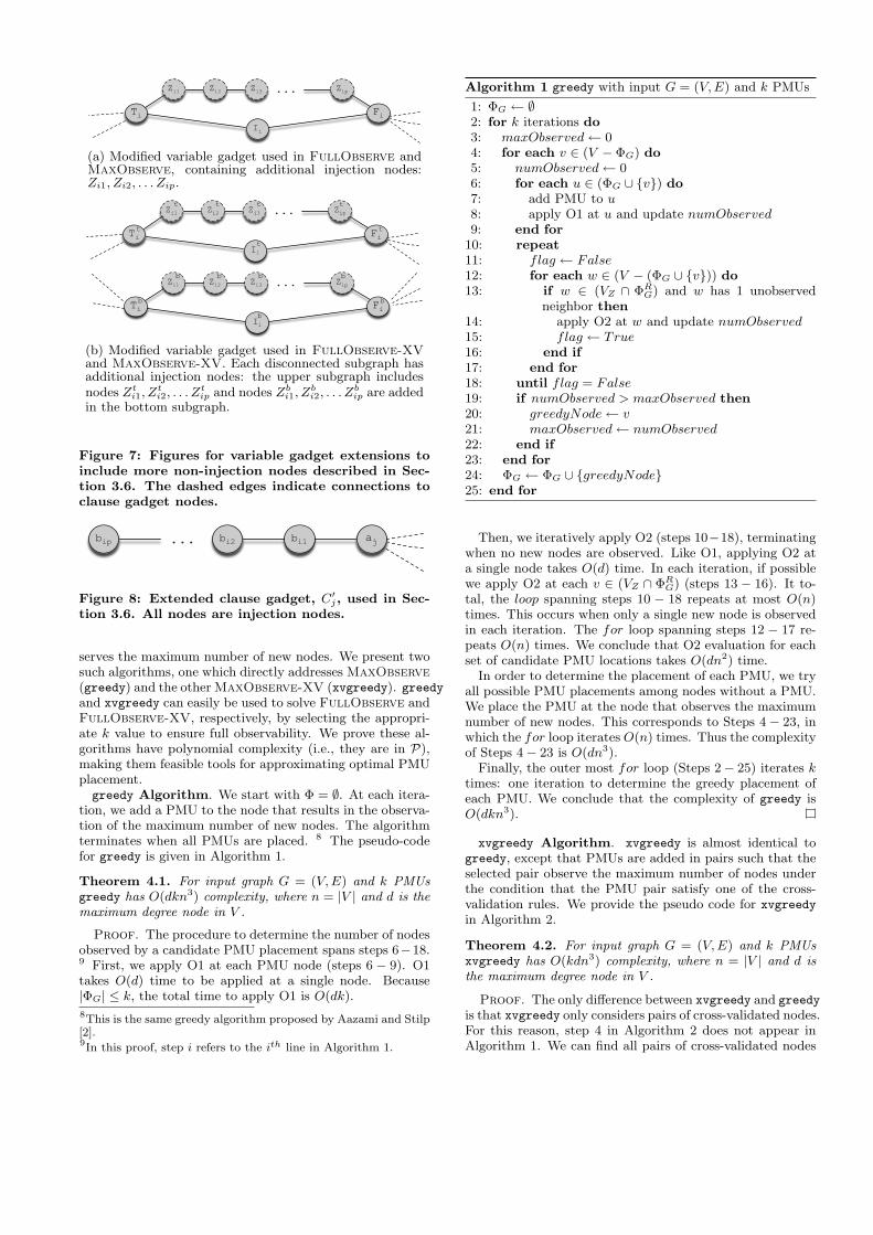
FiTiIi

Zi1 ...Zi2 ZipZi3

(a) Modified variable gadget used in FullObserve andMaxObserve, containing additional injection nodes:Zi1, Zi2, . . . Zip.

FiTiIi

Zi1 ...t

t

t

t

Zi2 ZipZi3t t t

FiTiIi

Zi1 ...b

b

b

b

Zi2 ZipZi3b b b

(b) Modified variable gadget used in FullObserve-XV

and MaxObserve-XV. Each disconnected subgraph hasadditional injection nodes: the upper subgraph includesnodes Zt

i1, Zt

i2, . . . Zt

ip and nodes Zb

i1, Zb

i2, . . . Zb

ip are addedin the bottom subgraph.

Figure 7: Figures for variable gadget extensions to

include more non-injection nodes described in Sec-

tion 3.6. The dashed edges indicate connections to

clause gadget nodes.

ajbi1bi2bip ...

Figure 8: Extended clause gadget, C�j, used in Sec-

tion 3.6. All nodes are injection nodes.

serves the maximum number of new nodes. We present twosuch algorithms, one which directly addresses MaxObserve

(greedy) and the other MaxObserve-XV (xvgreedy). greedyand xvgreedy can easily be used to solve FullObserve andFullObserve-XV, respectively, by selecting the appropri-ate k value to ensure full observability. We prove these al-gorithms have polynomial complexity (i.e., they are in P),making them feasible tools for approximating optimal PMUplacement.greedy Algorithm. We start with Φ = ∅. At each itera-

tion, we add a PMU to the node that results in the observa-tion of the maximum number of new nodes. The algorithmterminates when all PMUs are placed. 8 The pseudo-codefor greedy is given in Algorithm 1.

Theorem 4.1. For input graph G = (V, E) and k PMUs

greedy has O(dkn3) complexity, where n = |V | and d is the

maximum degree node in V .

Proof. The procedure to determine the number of nodesobserved by a candidate PMU placement spans steps 6−18.9 First, we apply O1 at each PMU node (steps 6 − 9). O1takes O(d) time to be applied at a single node. Because|ΦG| ≤ k, the total time to apply O1 is O(dk).8This is the same greedy algorithm proposed by Aazami and Stilp[2].9In this proof, step i refers to the ith line in Algorithm 1.

Algorithm 1 greedy with input G = (V, E) and k PMUs

1: ΦG ← ∅2: for k iterations do

3: maxObserved ← 04: for each v ∈ (V − ΦG) do

5: numObserved ← 06: for each u ∈ (ΦG ∪ {v}) do

7: add PMU to u8: apply O1 at u and update numObserved9: end for

10: repeat

11: flag ← False12: for each w ∈ (V − (ΦG ∪ {v})) do

13: if w ∈ (VZ ∩ ΦR

G) and w has 1 unobservedneighbor then

14: apply O2 at w and update numObserved15: flag ← True16: end if

17: end for

18: until flag = False19: if numObserved > maxObserved then

20: greedyNode ← v21: maxObserved ← numObserved22: end if

23: end for

24: ΦG ← ΦG ∪ {greedyNode}25: end for

Then, we iteratively apply O2 (steps 10−18), terminatingwhen no new nodes are observed. Like O1, applying O2 ata single node takes O(d) time. In each iteration, if possiblewe apply O2 at each v ∈ (VZ ∩ ΦR

G) (steps 13 − 16). It to-tal, the loop spanning steps 10 − 18 repeats at most O(n)times. This occurs when only a single new node is observedin each iteration. The for loop spanning steps 12 − 17 re-peats O(n) times. We conclude that O2 evaluation for eachset of candidate PMU locations takes O(dn2) time.

In order to determine the placement of each PMU, we tryall possible PMU placements among nodes without a PMU.We place the PMU at the node that observes the maximumnumber of new nodes. This corresponds to Steps 4− 23, inwhich the for loop iterates O(n) times. Thus the complexityof Steps 4− 23 is O(dn3).

Finally, the outer most for loop (Steps 2− 25) iterates ktimes: one iteration to determine the greedy placement ofeach PMU. We conclude that the complexity of greedy isO(dkn3).

xvgreedy Algorithm. xvgreedy is almost identical togreedy, except that PMUs are added in pairs such that theselected pair observe the maximum number of nodes underthe condition that the PMU pair satisfy one of the cross-validation rules. We provide the pseudo code for xvgreedyin Algorithm 2.

Theorem 4.2. For input graph G = (V, E) and k PMUs

xvgreedy has O(kdn3) complexity, where n = |V | and d is

the maximum degree node in V .

Proof. The only difference between xvgreedy and greedyis that xvgreedy only considers pairs of cross-validated nodes.For this reason, step 4 in Algorithm 2 does not appear inAlgorithm 1. We can find all pairs of cross-validated nodes

Algorithm 2 xvgreedy with input G = (V, E) and k PMUs

1: ΦG ← ∅2: for k iterations do

3: maxObserved ← 04: C ← all cross-validated node pairs in (V − ΦG)5: for each {v1, v2} ∈ C do

6: numObserved ← 07: for each u ∈ (ΦG ∪ {v1, v2}) do

8: add PMU to v1 and v2

9: apply O1 at u and update numObserved10: end for

11: repeat

12: flag ← False13: for each w ∈ (V − (ΦG ∪ {v1, v2})) do

14: if w ∈ (VZ ∩ ΦR

G) and w has 1 unobservedneighbor then

15: apply O2 at w and update numObserved16: flag ← True17: end if

18: end for

19: until flag = False20: if numObserved > maxObserved then

21: greedyNodes ← {v1, v2}22: maxObserved ← numObserved23: end if

24: end for

25: ΦG ← ΦG ∪ greedyNodes26: end for

in O(d2n) time. We do so by implementing a breadth-firstsearch at each v ∈ (V − ΦG) but stopping at a depth of 2.This takes O(d2) time for each node and since O(n) searchesare executed, step 4 takes O(d2n) time.

Because all other parts of Algorithm 1 and Algorithm 2 arenearly identical – Algorithm 2 adds PMUs in pairs while Al-gorithm 1 adds PMUs one-at-a-time – we are able to directlyapply the analysis from Theorem 4.1 in this proof. There-fore, we conclude the complexity of xvgreedy is O(k(d2n +dn3)) = O(dkn3).

5. SIMULATIONSTopologies. We evaluate our approximation algorithms

using simulations over IEEE topologies as well as syntheticones. For IEEE topologies, we use bus systems 14, 30, 57,and 118 10. The bus system number indicates the numberof nodes in the graph (e.g., bus system 57 has 57 nodes).Synthetic graphs are then generated based on each of thesetopologies, and are used to quantify the performance of ourgreedy approximations.

Since observability is determined by the connectivity ofthe graph, we use the degree distribution of IEEE topolo-gies as the template for generating our synthetic graphs. Asynthetic topology is generated from a given IEEE graph byrandomly “swapping” edges in the IEEE graph. Specifically,we select a random v ∈ V and then pick a random u ∈ Γ(v).Let u have degree du. Next, we select a random w /∈ Γ(v)with degree dw = du − 1. 11 Finally, we remove edge (v, u)and add (v, w), thereby preserving the node degree distribu-tion. We continue this swapping procedure until the original

10http://www.ee.washington.edu/research/pstca/11Here “random” means uniformly at random.

graph and generated graph share no edges, and then returnthe resulting graph.

Evaluation Methods. We are interested in evaluatinghow close our algorithms are to the optimal PMU place-ment. Thus, when computationally possible (for a givenk) we use brute-force algorithms to iterate over all possibleplacements of k PMUs in a given graph and select the bestPMU placement. When the brute-force algorithm is compu-tationally infeasible, we present only the performance of thegreedy algorithm. In what follows, the output of the brute-force algorithm is denoted optimal, and when we requirecross-validation it is denoted xvoptimal.

We present three different simulations in Section 5.1-5.3.In Section 5.1 we consider performance as a function of thenumber of PMUs, and in Section 5.2 we investigate the per-formance impact of the number of zero-injection nodes inthe network. These two sections are performed over sets ofsynthetic graphs. We conclude in Section 5.3 where we com-pare these results to the performance over the actual IEEEgraphs.

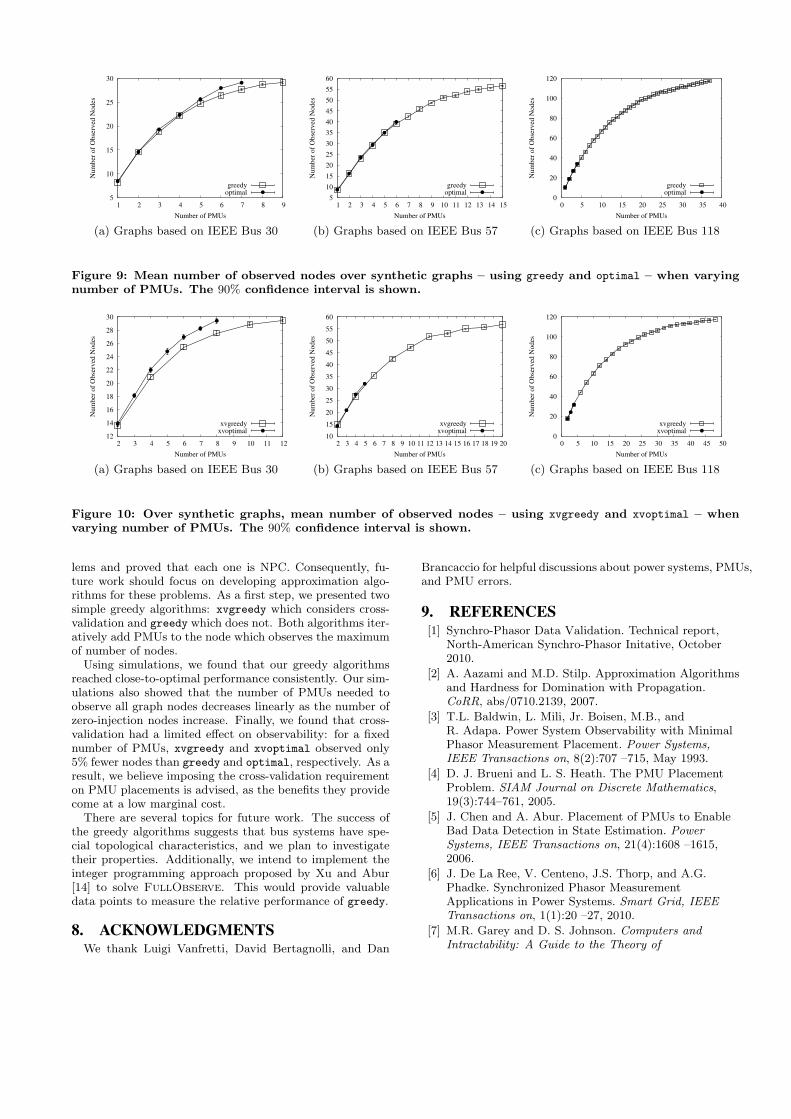
5.1 Simulation 1: Impact of Number of PMUsIn the first simulation scenario we vary the number of

PMUs and determine the number of observed nodes in thesynthetic graph. Each data point is generated as follows.For a given number of PMUs, k, we generate a graph, placek PMUs on the graph, and then determine the number of ob-served nodes. We continue this procedure until [0.9(x), 1.1(x)]– where x is the mean number of observed nodes using kPMUs – falls within the 90% confidence interval.

In addition to generating a topology, for each syntheticgraph we determined the members of VI , VZ . These nodesare specified for the original graphs in the IEEE bus systemdatabase. Thus, we randomly map each node in the IEEEnetwork to a node in the synthetic network with the samedegree, and then match their membership to either VI orVZ .

We present here results for solving MaxObserve andMaxObserve-XV. The number of nodes observed given k,using greedy and optimal, are shown in Figure 9, and Fig-ure 10 shows this number for xvgreedy and xvoptimal. Inboth sets of plots we show 90% confidence intervals. Weomit results for graphs based on IEEE bus 14 because thesame trends are observed.

Our greedy algorithms perform well. On average, greedyis within 98.6% of optimal, is never below 94% of opti-mal, and in most cases gives the optimal result. Likewise,xvgreedy is never less than 94% of xvoptimal and on av-erage is within 97% of xvoptimal. In about about half thecases xvgreedy gives the optimal result. These results sug-gest that despite the complexity of the problems, a greedyapproach can return high-quality results. Note, however,that these statistics do not include performance over largetopologies (i.e., IEEE graphs 57, 118) when k is large. It isan open question whether the greedy algorithms used herewould do well for larger graphs.

Surprisingly, when we compare our results with and with-out the cross-validation requirement, we find that the cross-validation constraints do not have a significant effect on thenumber of observed nodes for the same k. Our experimentsshow that on average xvoptimal observed only 5% fewernodes than optimal. Similarly, on average xvgreedy ob-serves 5.7% fewer nodes than greedy. This suggests that

the cost of imposing the cross-validation requirement is low,with the clear gain of ensuring PMU correctness across thenetwork.

5.2 Simulation 2: Impact of Number of Zero-Injection Nodes

Next, we examine the impact of the number of zero-injectionnodes (|VZ |) on algorithm performance. For each syntheticgraph, we run our algorithms for increasing values of |VZ |and determine the minimum number of PMUs needed toobserve all nodes in the graph (k∗). For each z := |VZ |,we select z nodes uniformly at random to be zero-injection,and the rest are in VI . Because we compute k∗ here, we solveFullObserve and FullObserve-XV, rather than MaxOb-

serve and MaxObserve-XV as in Simulation 1.We generate each data point using a similar procedure to

the one described in Section 5.1. For each z, we generatea graph and determine k∗. We then compute k∗, the meanvalue of k∗ using |VZ | = z. We continue this procedure until[0.9(k∗), 1.1(k∗)] falls within the 90% confidence interval.

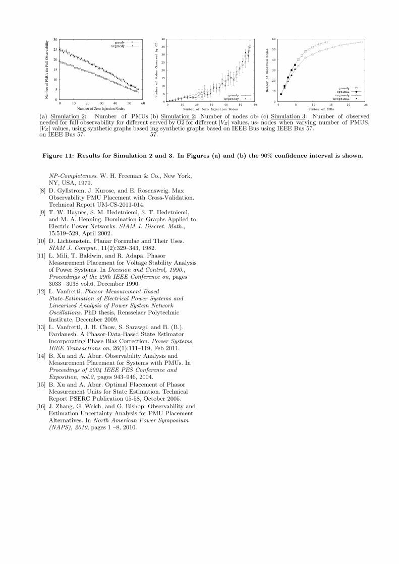
Figure 11(a) shows the simulation results for solving Ful-

lObserve and FullObserve-XV on synthetic graphs mod-eled by IEEE bus 57. Results for other topologies consideredhere (i.e., 14, 30 and 118) followed the same trend and arethus omitted. Due to the exponential running time of op-timal and xvoptimal, we present here only results of ourgreedy algorithms.

As expected, increasing the number of zero-injection nodes– for both greedy and xvgreedy – reduces the number ofPMUs required for full observability. More zero-injectionnodes allow O2 to be applied more frequently (Figure 11(b)),thereby increasing the number of observed nodes without us-ing more PMUs. In fact, we found the relationship between|VZ | to the greedy estimate of k∗ to be linear.

The gap in k∗ between greedy and xvgreedy decreases asz grows. greedy and xvgreedy observe a similar number ofnodes via O2 across all z values: the mean absolute differ-ence in the number of nodes observed by O2 between thetwo algorithms is only 1.66 nodes (equivalently, less than3% of observed nodes). Thus, as z grows the number ofnodes observed by O2 accounts for an increasing propor-tion of all observed nodes (Figure 11(b)), causing the gapbetween greedy and xvgreedy to shrink.

5.3 Simulation 3: Synthetic vs Actual IEEEGraphs

In this section, we compare our results with the perfor-mance over the original IEEE systems. We assign nodes toVZ and VI as specified in the IEEE database files. Our re-sults indicate that the trends we observed over the syntheticgraphs apply as well to real topologies.

Figure 11(c) shows the number of observed nodes for thegreedy, xvgreedy, optimal, and xvoptimal algorithms forIEEE bus system 57. greedy and xvgreedy observe nearlyas many nodes as the corresponding optimal solution. Inmany cases, greedy yields the optimal placement. Similarly,as with the synthetic graphs, the number of PMUs requiredto observe all nodes decreases linearly as |VZ | increases. 12

To compare the actual values for synthetic graphs to thoseover IEEE graphs, we took the mean absolute difference

12The same trends are observed using IEEE bus systems 14, 30,and 118.

greedy xvgreedy optimal xvoptimal

Simulation 1 4% 4.6% 6% 7.6%Simulation 2 9.1% 16.1% N/A N/A

Table 1: Mean absolute difference between the

computed values from synthetic graphs and IEEE

graphs, normalized by the result for the synthetic

graph.

between the results, and normalized by the result for thesynthetic graph. For example, let nk be the mean number ofobserved nodes using greedy over all synthetic graphs withinput k, and let nG,k be the output of greedy for IEEE graphG and k. We compute nd,k = (|nk − nG,k|)/nk. Finally, wecalculate the mean over all nd,k. This process is done foreach algorithm we evaluate. The resulting statistics can befound in Table 1. The small average difference between thesynthetic graphs and the actual IEEE topologies suggeststhat the node degree distribution of the IEEE graph is aneffective feature for generating similar synthetic graphs.

6. RELATED WORKFullObserve is well-studied [3, 4, 9, 11, 14]. Haynes et

al. [9] and Brueni and Heath [4] both prove FullObserve isNPC. However, their proofs make the unrealistic assumptionthat all nodes are zero-injection. We drop this assumptionand thereby generalize their NPC results for FullObserve.Additionally, we leverage the proof technique from Brueniand Heath [4] in the NPC proofs for all four of our place-ment problems, although our proofs differ considerably inthe details.

In the power systems literature, Xu and Abur [14, 15] useinteger programming to solve FullObserve, while Baldwinet al. [3] and Mili et al. [11] use simulated annealing tosolve the same problem. All of these works allow nodesto be either zero-injection or non-zero-injection. However,these papers make no mention that FullObserve is NPC,i.e., they do not characterize the fundamental complexity ofthe problem.

Aazami and Stilp [2] investigate approximation algorithmsfor FullObserve. They derive a hardness approximation

threshold of 2log1−�n. Also they prove that in the worst case,

greedy from Section 4 does no better Θ(n) of the optimalsolution. However, this approximation ratio assumes thatall nodes are zero-injection.

Chen and Abur [5] and Vanfretti et al. [13] both studythe problem of bad PMU data. Chen and Abur [5] formu-late their problem differently than FullObserve-XV andMaxObserve-XV. They consider graphs that are alreadyfully observable and then add PMUs to the system to makeall existing PMU measurements non-critical (a critical mea-surement is one in which the removal of a PMU makes thesystem no longer fully observable). Vanfretti et al. [13] de-fine the cross-validation rules used in this paper. They alsoderive a lower bound on the number of PMUs needed toensure all PMUs are cross-validated and the system is fullyobservable.

7. CONCLUSIONS AND FUTURE WORKIn this work, we formulated four PMU placement prob-

5

10

15

20

25

30

1 2 3 4 5 6 7 8 9

Nu

mb

er o

f O

bse

rved

No

des

Number of PMUs

greedyoptimal

(a) Graphs based on IEEE Bus 30

5

10

15

20

25

30

35

40

45

50

55

60

1 2 3 4 5 6 7 8 9 10 11 12 13 14 15

Nu

mb

er o

f O

bse

rved

No

des

Number of PMUs

greedyoptimal

(b) Graphs based on IEEE Bus 57

0

20

40

60

80

100

120

0 5 10 15 20 25 30 35 40

Nu

mb

er o

f O

bse

rved

No

des

Number of PMUs

greedyoptimal

(c) Graphs based on IEEE Bus 118

Figure 9: Mean number of observed nodes over synthetic graphs – using greedy and optimal – when varying

number of PMUs. The 90% confidence interval is shown.

12

14

16

18

20

22

24

26

28

30

2 3 4 5 6 7 8 9 10 11 12

Num

ber

of

Ob

serv

ed N

od

es

Number of PMUs

xvgreedyxvoptimal

(a) Graphs based on IEEE Bus 30

10

15

20

25

30

35

40

45

50

55

60

2 3 4 5 6 7 8 9 10 11 12 13 14 15 16 17 18 19 20

Num

ber

of

Ob

serv

ed N

od

es

Number of PMUs

xvgreedyxvoptimal

(b) Graphs based on IEEE Bus 57

0

20

40

60

80

100

120

0 5 10 15 20 25 30 35 40 45 50

Num

ber

of

Ob

serv

ed N

od

es

Number of PMUs

xvgreedyxvoptimal

(c) Graphs based on IEEE Bus 118

Figure 10: Over synthetic graphs, mean number of observed nodes – using xvgreedy and xvoptimal – when

varying number of PMUs. The 90% confidence interval is shown.

lems and proved that each one is NPC. Consequently, fu-ture work should focus on developing approximation algo-rithms for these problems. As a first step, we presented twosimple greedy algorithms: xvgreedy which considers cross-validation and greedy which does not. Both algorithms iter-atively add PMUs to the node which observes the maximumof number of nodes.

Using simulations, we found that our greedy algorithmsreached close-to-optimal performance consistently. Our sim-ulations also showed that the number of PMUs needed toobserve all graph nodes decreases linearly as the number ofzero-injection nodes increase. Finally, we found that cross-validation had a limited effect on observability: for a fixednumber of PMUs, xvgreedy and xvoptimal observed only5% fewer nodes than greedy and optimal, respectively. As aresult, we believe imposing the cross-validation requirementon PMU placements is advised, as the benefits they providecome at a low marginal cost.

There are several topics for future work. The success ofthe greedy algorithms suggests that bus systems have spe-cial topological characteristics, and we plan to investigatetheir properties. Additionally, we intend to implement theinteger programming approach proposed by Xu and Abur[14] to solve FullObserve. This would provide valuabledata points to measure the relative performance of greedy.

8. ACKNOWLEDGMENTSWe thank Luigi Vanfretti, David Bertagnolli, and Dan

Brancaccio for helpful discussions about power systems, PMUs,and PMU errors.

9. REFERENCES[1] Synchro-Phasor Data Validation. Technical report,

North-American Synchro-Phasor Initative, October2010.

[2] A. Aazami and M.D. Stilp. Approximation Algorithmsand Hardness for Domination with Propagation.CoRR, abs/0710.2139, 2007.

[3] T.L. Baldwin, L. Mili, Jr. Boisen, M.B., andR. Adapa. Power System Observability with MinimalPhasor Measurement Placement. Power Systems,

IEEE Transactions on, 8(2):707 –715, May 1993.[4] D. J. Brueni and L. S. Heath. The PMU Placement

Problem. SIAM Journal on Discrete Mathematics,19(3):744–761, 2005.

[5] J. Chen and A. Abur. Placement of PMUs to EnableBad Data Detection in State Estimation. Power

Systems, IEEE Transactions on, 21(4):1608 –1615,2006.

[6] J. De La Ree, V. Centeno, J.S. Thorp, and A.G.Phadke. Synchronized Phasor MeasurementApplications in Power Systems. Smart Grid, IEEE

Transactions on, 1(1):20 –27, 2010.[7] M.R. Garey and D. S. Johnson. Computers and

Intractability: A Guide to the Theory of

0

5

10

15

20

25

30

0 10 20 30 40 50 60

Nu

mb

er o

f P

MU

s fo

r F

ull

Obse

rvab

ilit

y

Number of Zero Injection Nodes

greedyxvgreedy

(a) Simulation 2: Number of PMUsneeded for full observability for different|VZ | values, using synthetic graphs basedon IEEE Bus 57.

0

5

10

15

20

25

30

35

40

0 10 20 30 40 50 60

Number

of No

des

Observ

ed b

y O2

Number of Zero Injection Nodes

greedyxvgreedy

(b) Simulation 2: Number of nodes ob-served by O2 for different |VZ | values, us-ing synthetic graphs based on IEEE Bus57.

0

10

20

30

40

50

60

0 5 10 15 20 25

Numb

er of

Obse

rved N

odes

Number of PMUs

greedyoptimal

xvgreedyxvoptimal

(c) Simulation 3: Number of observednodes when varying number of PMUS,using IEEE Bus 57.

Figure 11: Results for Simulation 2 and 3. In Figures (a) and (b) the 90% confidence interval is shown.

NP-Completeness. W. H. Freeman & Co., New York,NY, USA, 1979.

[8] D. Gyllstrom, J. Kurose, and E. Rosensweig. MaxObservability PMU Placement with Cross-Validation.Technical Report UM-CS-2011-014.

[9] T. W. Haynes, S. M. Hedetniemi, S. T. Hedetniemi,and M. A. Henning. Domination in Graphs Applied toElectric Power Networks. SIAM J. Discret. Math.,15:519–529, April 2002.

[10] D. Lichtenstein. Planar Formulae and Their Uses.SIAM J. Comput., 11(2):329–343, 1982.

[11] L. Mili, T. Baldwin, and R. Adapa. PhasorMeasurement Placement for Voltage Stability Analysisof Power Systems. In Decision and Control, 1990.,

Proceedings of the 29th IEEE Conference on, pages3033 –3038 vol.6, December 1990.

[12] L. Vanfretti. Phasor Measurement-Based

State-Estimation of Electrical Power Systems and

Linearized Analysis of Power System Network

Oscillations. PhD thesis, Rensselaer PolytechnicInstitute, December 2009.

[13] L. Vanfretti, J. H. Chow, S. Sarawgi, and B. (B.).Fardanesh. A Phasor-Data-Based State EstimatorIncorporating Phase Bias Correction. Power Systems,

IEEE Transactions on, 26(1):111–119, Feb 2011.[14] B. Xu and A. Abur. Observability Analysis and

Measurement Placement for Systems with PMUs. InProceedings of 2004 IEEE PES Conference and

Exposition, vol.2, pages 943–946, 2004.[15] B. Xu and A. Abur. Optimal Placement of Phasor

Measurement Units for State Estimation. TechnicalReport PSERC Publication 05-58, October 2005.

[16] J. Zhang, G. Welch, and G. Bishop. Observability andEstimation Uncertainty Analysis for PMU PlacementAlternatives. In North American Power Symposium

(NAPS), 2010, pages 1 –8, 2010.