Transmission algorithm for video streaming over cellularnetworks

Y. Falik Æ A. Averbuch Æ U. Yechiali

� Springer Science+Business Media, LLC 2009

Abstract 2.5G and 3G cellular networks are becoming

more widespread and the need for value added services

increases rapidly. One of the key services that operators

seek to provide is streaming of rich multimedia con-

tent. However, network characteristics make the use of

streaming applications very difficult with an unacceptable

quality of service (QoS). The 3GPP standardization body

has standardized streaming services that will benefit oper-

ators and users. There is a need for a mechanism that will

enable a good quality multimedia streaming that uses the

3GPP standard. This paper describes an adaptive streaming

algorithm that uses the 3GPP standard. It improves sig-

nificantly the QoS in varying network conditions while

monitoring its performance using queueing methodologies.

The algorithm utilizes the available buffers on the route of

the streaming data in a unique way that guarantees high

QoS. The system is analytically modeled: the streaming

server, the cellular network and the cellular client are

modeled as cascaded buffers and the data is sequentially

streamed between them. The proposed Adaptive streaming

algorithm (ASA) controls these buffers’ occupancy levels

by controlling the transmission and the encoding rates of

the streaming server to achieve high QoS for the streaming.

It overcomes the inherent fluctuations of the network

bandwidth. The algorithm was tested on General Packet

Radio Service (GPRS), Enhanced Data rates for GSM

Evolution (EDGE) and Universal Mobile Telecommuni-

cation System (UMTS) networks. The results showed

substantial improvements over other standard streaming

methods used today.

Keywords Video transmission � Cellular �Modeling, 3GPP � QoS � Adaptive streaming

1 Introduction

Streaming video is becoming a common application in 2.5

and 3rd generation cellular networks. The need for value

added services in cellular networks is growing rapidly and

thus the 3rd Generation Partnership Project (3GPP), which

defines the standard for the 3rd generation cellular net-

works, dedicated a special work group for streaming video

[1, 2]. The problem is the low and fluctuated bandwidth of

the network that makes a use of streaming applications—

while maintaining steady and smooth stream with high

(QoS)—very difficult. There are several reasons for band-

width fluctuations:

Network load: In each cell, there is a limited amount of

channel resources divided between voice and data

sessions. The variation in the number of voice and data

sessions and their required resources cause the network

to constantly change the channel resources allocated for

a streaming session. There is no guarantee for a steady

constant bit allocation.

Radio network conditions: The radio network conditions

may vary during a streaming session because of fading

and interference. In order to prevent a packet loss, the

Y. Falik � A. Averbuch (&)

School of Computer Science, Tel Aviv University,

Tel Aviv 69978, Israel

e-mail: amir@math.tau.ac.il

URL: http://www.math.tau.ac.il/*amir

U. Yechiali

Department of Statistics and Operations Research,

School of Mathematical Sciences, Tel Aviv University,

Tel Aviv 69978, Israel

123

Wireless Netw

DOI 10.1007/s11276-009-0214-x

network has a bounded retransmission mechanism,

which resends a packet whenever a client fails to receive

it. Another mechanism is the forward error correction

(FEC) that adds more bits to the data in order to prevent

data loss. The FEC level is controlled by the network to

match varying network conditions. This results in

available bandwidth fluctuation causing congestions

and delays.

Handovers: Another scenario that causes bandwidth to

fluctuate or even momentarily stop is handovers. When a

user moves from the coverage area of one network into

another, it is called intra-network handovers. When a

user moves from the coverage area of a cell to another,

the system must provide the capability for that user to

remain ‘‘in touch’’ even while breaking the connection

with one base station and establishing another connec-

tion with another base station. This operation is called

inter-network handover.

Another problem that makes streaming in a steady

bitrate difficult is finding out the network bandwidth. There

is no standard way to acquire bandwidth information from

the network. Therefore, we have to rely on reports from the

client and it has an unknown delay. The client reports only

on an integer number of packets that were received. Usu-

ally, to avoid packetization overhead, the size of the packet

is very large. Therefore, according to our experience with

different telephone type and different cellular network, one

packet may be received after up to maximum of 2 s. Thus,

the bandwidth can be measured only in large discrete steps

with coarse resolution.

These problems cause the operator to utilize only a

fraction of its bandwidth on the one hand, and cause the

end user to experience a poor video quality on the other

hand.

Figure 1 illustrates the UMTS network architecture. The

streaming server resides either in the Internet (PDN in

Fig. 1) or usually in the operator premises just before the

Gateway GPRS Support Node (GGSN) that acts as a

gateway between the UMTS wireless data network and

other networks such as the Internet or private networks.

The data is passed from the GGSN to the Serving GPRS

Support Node (SGSN) that does the full set of inter-

working with the connected radio network and then to the

Radio Network Controller (RNC), which is the governing

element in the UMTS radio access network (UTRAN),

responsible for control of the base stations (Node-Bs) that

are connected to the controller. The RNC carries out radio

resource management, some of the mobility management

functions and is the point where encryption is done before

user’s data is sent to and from the mobile.

In order to enable handovers between base stations and

packet retransmission the data is stored in the buffers of

SGSN and RNC (see Fig. 2). These buffers are reallocated

for each data session. In this paper, these buffers are con-

sidered as a single buffer ‘‘The Network buffer’’. Although

the streaming server does not control the network buffer

directly, its behavior during the streaming session is critical

in assuring a smooth data stream and a good QoS.

In order to enable a good quality and a smooth multi-

media streaming there is a need for adaptive streaming.

Fig. 1 UMTS architecture.

Left: radio access network.

Middle: core network. Right:packet-data/telephone network

Wireless Netw

123

The use of constant bit rate media as it comes from the

encoder on a varying bit rate channels is not recommended.

The term adaptive here means that a streaming service is

able to adapt to varying network conditions. Examples of

such variations include variations in throughput, delay and

intra/inter-operator roaming to networks with or without

QoS support.

These situations are not very critical for non-real time

traffic such as downloading, ftp, browsing. However, they

become critical for continuous media transmission, such as

streaming, where the user experience drops if the service

loses its inherent properties of continuity, synchronization

and real-timeness. For instance, continuous (or pause-less)

playback is the number one requirement for a successful

streaming service. When the network throughput is con-

stantly varying during a session, the effect on the end user’s

client is that of a frozen picture, pauses in the audio/video

playback, continuous rebufferings (i.e., re-loading from the

streaming server a sufficient amount of media data to be

streamed with no interruptions) and bad media quality

(caused by packet losses caused by network buffers

overflow).

Adaptive streaming avoids the above phenomena and

ensures pause-less playback to the end user, yielding a

superior user experience compared to conventional

streaming. The streaming server uses adaptive streaming

by changing the media and the streaming rates. Streaming

rate is the rate in which the media is sent from the

streaming server to the network. Media rate is the rate in

which the media is played (e.g., 32 kbps video means that

each second of compressed video is described by 32 kb).

The media rate can be changed in live encoding (online) by

changing the encoding rate, or in offline by keeping a set of

media streams of the same content encoded at different bit

rates and performing seamless switch between these dif-

ferent media streams. For example, if a streaming session

starts at 64 kbps with good network throughput, and sub-

sequently the network throughput halves, the streaming

server can switch to a lower bit rate stream (e.g., 32 kbps)

to guarantee pause-less playback and avoid network buffers

overflow that can cause packet losses and bad QoS. The

server can switch back to the 64 kbps media stream when

network conditions improve.

The proposed adaptive media streaming performance is

analyzed using methods from queueing theory. For this

analysis, the data flow in a streaming session (Fig. 3) is

modeled as having one input process (the application

server—left of the figure) and two serially connected

Fig. 2 UMTS network buffer—

portion of Fig. 1 that is of

interest to this paper

Fig. 3 The modeled

multimedia streaming:

functional entities

Wireless Netw

123

queues—the mobile network buffer (middle of the figure)

and the client buffer (right of the figure). The data is

delivered from the streaming server to the network, where

it is queued (network buffer) and served (transmitted),

arriving at the client where it is queued (client jitter buffer)

and served (played).

The data flow from the streaming server is controlled.

The mobile network buffer queue serves (transmits) the

data in a rate that is modeled as a Poisson process [3]. The

client queue (Fig. 3) serves (plays) the data in its encoded

bit rate. The control mechanism for the streaming server

and the performance analysis of the mobile network and

the client queues are the subject of this paper.

The physical implementation of the model is illustrated

in Fig. 2. The streaming server resides in the PDN, the

network buffer is in the SGSN and RNC and the client

buffer is in the client.

This paper introduces a model for maintaining a steady

QoS for streaming video as described schematically in

Fig. 3. An algorithm, which is best-fit for this prob-

lem model, is suggested. The algorithm maximizes the

streaming session bandwidth utilization while minimizing

delays and packet loss. The algorithm can be used on any

3GPP standard client that sends RTCP reports [4]. It was

tested on UMTS, EDGE and GPRS networks.

The structure of the paper is as follows. In Sect. 2, we

present related work. In Sect. 3, we describe an adaptive

streaming algorithm to be used in the streaming server to

achieve better QoS. The stochastic performance of the

algorithm is described in Sect. 4. Experimental and simu-

lation results on several cellular networks are presented in

Sect. 5.

2 Related work

2.1 Congestion control

In cellular networks, the low and fluctuated bandwidth make

streaming applications—while maintaining steady and

smooth stream with high QoS—a very difficult task. Con-

gestion control is aimed at solving this problem by adapting

the streaming rate to the oscillatory network conditions.

The standardized solution in 3GPP Release 6 to handle

adaptive streaming is described in [5, 6]. The 3GPP PSS

specifications introduce signaling from the client to the

server, which allows the server to have the information it

needs in order to best choose both transmission rate

and media encoding rate at any time. An adaptive video

streaming system, which is compliant with PSS, is

described in [7]. This system performs well, but it is dif-

ferent from the proposed algorithm. It does not provide

theoretical infrastructure for stream modeling.

The rate adaptation problem is termed curve control [2].

The playout curve shows the cumulative size of the data the

decoder has processed by a given time from the client

buffer. The encoding curve indicates the progress of data

generation if the media encoder runs in real-time. The

transmission curve shows the cumulative size of the data

sent out by the server at a given time. The reception curve

shows the cumulative size of the data received in the cli-

ent’s buffer at a given time.

The distance between the transmission and the reception

curves corresponds to the size of the data in the network

buffer and the distance between the reception and playout

curves corresponds to the size of the data in the client

buffer. Curve control here means a limited constrain on the

distance between two curves (e.g., by a maximum size of

the data, or a maximum delay). This problem is equivalent

to controlling the network and the client buffers. However,

there is no specific suggestion for choosing the transmis-

sion rate and the media encoding rate, and there is no

treatment how to handle a client that does not support

3GPP Release 6 signaling.

A widely popular rate control scheme over wired net-

works is equation-based rate control ([8, 9]), also known as

the TCP friendly rate control (TFRC). There are basically

three main advantages for a rate control that uses TFRC:

first, it does not cause network instability, which means

that congestion collapse is avoided. More specifically,

TFRC mechanism monitors the status of the network and

every time that congestion is detected it adjusts the sending

rates of the streaming applications. Second, it is fair for

TCP flows, which are the dominant source of traffic on the

Internet. Third, the TFRC’s rate fluctuation is lower than

TCP, thus, making it more appropriate for streaming

applications which require constant video quality.

A widely popular model for TFRC is described by

T ¼ kS

RTTffiffiffi

pp

where T is the sending rate, S is the packet size, RTT is the

end-to-end round trip time, p is the end-to-end packet loss

rate and k is a constant factor between 0.7 and 1.3,

depending on the particular derivation of the TFRC

equation.

The use of TFRC for streaming video over wireless

networks is described in [10]. It resolves two TFRC diffi-

culties: first, TFRC assumes that packet loss in wired net-

works is primarily due to congestion and as such it is not

applicable to wireless networks in which the bulk of packet

loss is due to error in the physical layer. Second, TFRC

does not fully utilize the network channel. It resolves it by

multiple TFRC connections that results in full utilization of

the network channel. However, it is not possible to use

multiple connections in standard 3GPP streaming clients.

Wireless Netw

123

The use of TFRC for streaming video over UMTS is

given in [11]. The round trip time and the packet loss rate

are estimated using the standard real time control protocol

(RTCP) RR. The problem of under utilization of one TFRC

connection remains.

2.2 Video scalability

Adaptive streaming enables to achieve a better QoS com-

pared to conventional streaming. The streaming server uses

adaptive streaming by changing the media rate and the

streaming rate. Media rate means the bit rate in which the

media is encoded/played. The media rate can be changed in

live encoding by changing the encoding bit rate or

by offline. Several approaches were suggested to enable

dynamic bit rate change:

MPEG-4 ([12]) simple scalable profile is an MPEG-4

tool which enables to change the number of frames per

second or the spatial resolution of the media. It encodes

the media in several dependent layers and determines the

media quality by adding or subtracting layers.

MPEG-4 Fine granularity scalability (FGS) is a type of

scalability where an enhancement layer can be truncated

into any number of bits that provides a corresponding

quality enhancement.

A different approach to handle varying encoding bit

rates is to use several independent versions of the same

media and to switch between these versions. The simplest

method is to switch between the versions in key-frames,

which are independent frames, that can be decoded inde-

pendently in any version. Another method, which switches

between media versions, creates dedicated P-frames (P-

frames are the predicted frames that code the difference

between two consecutive frames) that when they are

decoded in one version, then contiguous playing from a

different version ([13]) is enabled.

H264 SP-frames ([14]) are similar to switching P-frames

because they code the difference between frames for dif-

ferent media versions. However, the coding is lossless,

therefore, switching between media versions is done

without introducing any error to the video stream. The

system in [15], which is a variation of [7], presents a

streaming system that utilizes interleaved transmission for

real-time H264/AVC video in 3G wireless environments

without theoretical modeling.

3 The Adaptive Streaming Algorithm (ASA)

This section describes the proposed Adaptive Streaming

Algorithm (ASA) to be used in the streaming server.

A general description of the system is given in Fig. 4. The

streaming server controls two transmission parameters: the

streaming rate and the encoding rate.

In conventional streaming servers, these two rates are

equal to each other, which means that the video clip is

streamed at the same rate as it was encoded. The equality

of this rate imposes an unnecessary restriction on the sys-

tem, which causes sub-optimal utilization of the network

resources. In the proposed algorithm, this restriction is

removed. This enables a full utilization by flexible adap-

tation to the network resources.

The system is modeled in the following way: the

streaming server, the cellular network and the cellular

client are modeled as cascaded buffers (see Fig. 4), and the

data is passed between them sequentially. The goal of the

algorithm is to control all these buffers-occupancy levels

by controlling the transmission rate of the streaming server

and the decoding rate of the cellular client to achieve

streaming with high QoS.

3.1 Data flow and buffers

In the ASA model, all the functional entities of the mul-

timedia streaming are considered as buffers (see Fig. 4).

Three buffers are used:

Streaming server buffer: In an on-demand scenario, the

streaming server can use the video file as a buffer and

Fig. 4 Adaptive streaming data and a control flow diagram. The data

is passed between the Streaming server, NW and client buffers

according to specified rates. The client sends periodic RTCP reports

to the Streaming Server enabling to calculate the NW and the client

occupancy levels

Wireless Netw

123

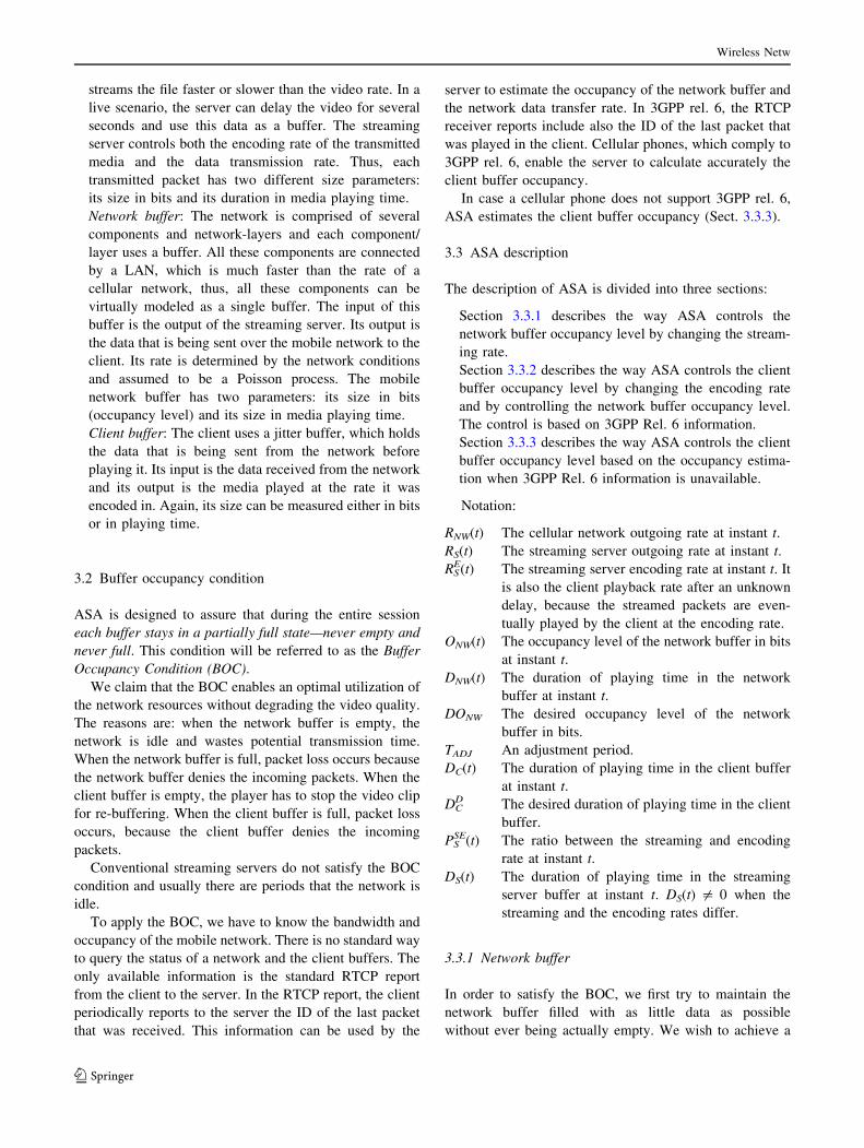
streams the file faster or slower than the video rate. In a

live scenario, the server can delay the video for several

seconds and use this data as a buffer. The streaming

server controls both the encoding rate of the transmitted

media and the data transmission rate. Thus, each

transmitted packet has two different size parameters:

its size in bits and its duration in media playing time.

Network buffer: The network is comprised of several

components and network-layers and each component/

layer uses a buffer. All these components are connected

by a LAN, which is much faster than the rate of a

cellular network, thus, all these components can be

virtually modeled as a single buffer. The input of this

buffer is the output of the streaming server. Its output is

the data that is being sent over the mobile network to the

client. Its rate is determined by the network conditions

and assumed to be a Poisson process. The mobile

network buffer has two parameters: its size in bits

(occupancy level) and its size in media playing time.

Client buffer: The client uses a jitter buffer, which holds

the data that is being sent from the network before

playing it. Its input is the data received from the network

and its output is the media played at the rate it was

encoded in. Again, its size can be measured either in bits

or in playing time.

3.2 Buffer occupancy condition

ASA is designed to assure that during the entire session

each buffer stays in a partially full state—never empty and

never full. This condition will be referred to as the Buffer

Occupancy Condition (BOC).

We claim that the BOC enables an optimal utilization of

the network resources without degrading the video quality.

The reasons are: when the network buffer is empty, the

network is idle and wastes potential transmission time.

When the network buffer is full, packet loss occurs because

the network buffer denies the incoming packets. When the

client buffer is empty, the player has to stop the video clip

for re-buffering. When the client buffer is full, packet loss

occurs, because the client buffer denies the incoming

packets.

Conventional streaming servers do not satisfy the BOC

condition and usually there are periods that the network is

idle.

To apply the BOC, we have to know the bandwidth and

occupancy of the mobile network. There is no standard way

to query the status of a network and the client buffers. The

only available information is the standard RTCP report

from the client to the server. In the RTCP report, the client

periodically reports to the server the ID of the last packet

that was received. This information can be used by the

server to estimate the occupancy of the network buffer and

the network data transfer rate. In 3GPP rel. 6, the RTCP

receiver reports include also the ID of the last packet that

was played in the client. Cellular phones, which comply to

3GPP rel. 6, enable the server to calculate accurately the

client buffer occupancy.

In case a cellular phone does not support 3GPP rel. 6,

ASA estimates the client buffer occupancy (Sect. 3.3.3).

3.3 ASA description

The description of ASA is divided into three sections:

Section 3.3.1 describes the way ASA controls the

network buffer occupancy level by changing the stream-

ing rate.

Section 3.3.2 describes the way ASA controls the client

buffer occupancy level by changing the encoding rate

and by controlling the network buffer occupancy level.

The control is based on 3GPP Rel. 6 information.

Section 3.3.3 describes the way ASA controls the client

buffer occupancy level based on the occupancy estima-

tion when 3GPP Rel. 6 information is unavailable.

Notation:

RNW(t) The cellular network outgoing rate at instant t.

RS(t) The streaming server outgoing rate at instant t.

RSE(t) The streaming server encoding rate at instant t. It

is also the client playback rate after an unknown

delay, because the streamed packets are even-

tually played by the client at the encoding rate.

ONW(t) The occupancy level of the network buffer in bits

at instant t.

DNW(t) The duration of playing time in the network

buffer at instant t.

DONW The desired occupancy level of the network

buffer in bits.

TADJ An adjustment period.

DC(t) The duration of playing time in the client buffer

at instant t.

DCD The desired duration of playing time in the client

buffer.

PSSE(t) The ratio between the streaming and encoding

rate at instant t.

DS(t) The duration of playing time in the streaming

server buffer at instant t. DS(t) = 0 when the

streaming and the encoding rates differ.

3.3.1 Network buffer

In order to satisfy the BOC, we first try to maintain the

network buffer filled with as little data as possible

without ever being actually empty. We wish to achieve a

Wireless Netw

123

constant occupancy level. The occupancy level ONW(t) is

affected by the network input and output rates. The

output rate RNW(t) is the network data output rate, which

is not controlled by our application. The input rate RS(t)

is the streaming server rate, which is fully controllable. It

is important to note that the video encoding rate RSE(t)

does not affect the network buffer occupancy level,

because the rate in which data enters the network buffer

is determined by the streaming server outgoing rate RS(t).

The video encoding rate RSE(t) determines the playback

rate of the video which affects the client and not the

network.

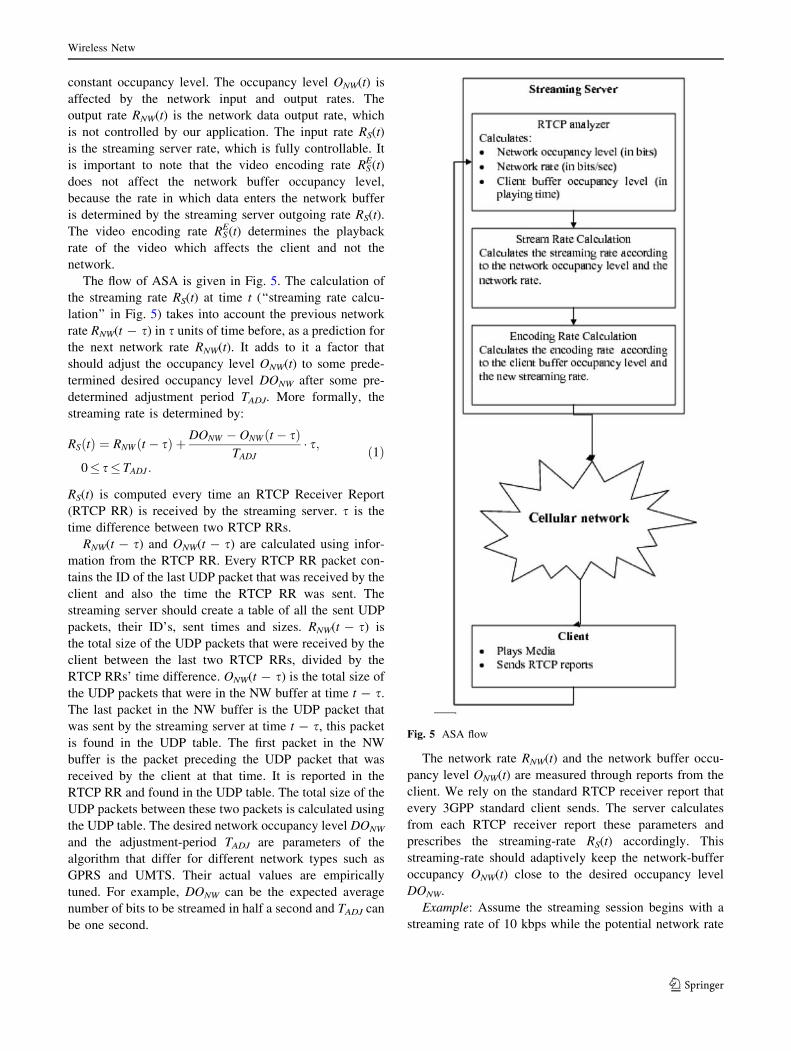
The flow of ASA is given in Fig. 5. The calculation of

the streaming rate RS(t) at time t (‘‘streaming rate calcu-

lation’’ in Fig. 5) takes into account the previous network

rate RNW(t - s) in s units of time before, as a prediction for

the next network rate RNW(t). It adds to it a factor that

should adjust the occupancy level ONW(t) to some prede-

termined desired occupancy level DONW after some pre-

determined adjustment period TADJ. More formally, the

streaming rate is determined by:

RSðtÞ ¼ RNWðt � sÞ þ DONW � ONWðt � sÞTADJ

� s;0� s� TADJ :

ð1Þ

RS(t) is computed every time an RTCP Receiver Report

(RTCP RR) is received by the streaming server. s is the

time difference between two RTCP RRs.

RNW(t - s) and ONW(t - s) are calculated using infor-

mation from the RTCP RR. Every RTCP RR packet con-

tains the ID of the last UDP packet that was received by the

client and also the time the RTCP RR was sent. The

streaming server should create a table of all the sent UDP

packets, their ID’s, sent times and sizes. RNW(t - s) is

the total size of the UDP packets that were received by the

client between the last two RTCP RRs, divided by the

RTCP RRs’ time difference. ONW(t - s) is the total size of

the UDP packets that were in the NW buffer at time t - s.

The last packet in the NW buffer is the UDP packet that

was sent by the streaming server at time t - s, this packet

is found in the UDP table. The first packet in the NW

buffer is the packet preceding the UDP packet that was

received by the client at that time. It is reported in the

RTCP RR and found in the UDP table. The total size of the

UDP packets between these two packets is calculated using

the UDP table. The desired network occupancy level DONW

and the adjustment-period TADJ are parameters of the

algorithm that differ for different network types such as

GPRS and UMTS. Their actual values are empirically

tuned. For example, DONW can be the expected average

number of bits to be streamed in half a second and TADJ can

be one second.

The network rate RNW(t) and the network buffer occu-

pancy level ONW(t) are measured through reports from the

client. We rely on the standard RTCP receiver report that

every 3GPP standard client sends. The server calculates

from each RTCP receiver report these parameters and

prescribes the streaming-rate RS(t) accordingly. This

streaming-rate should adaptively keep the network-buffer

occupancy ONW(t) close to the desired occupancy level

DONW.

Example: Assume the streaming session begins with a

streaming rate of 10 kbps while the potential network rate

Fig. 5 ASA flow

Wireless Netw

123

is a constant 30 kbps. The streaming server cannot know

the potential network rate, but since the network buffer will

be empty after the first RTCP report, it raises the streaming

rate. Then, data will start to accumulate in the network

buffer. Subsequently, the network buffer reaches its desired

occupancy level and then the streaming rate will decrease

until it will equate the network rate. Then, the network

buffer will remain at the constant desired occupancy level.

Throughout the session, a change in the network

potential rate will only appear in the actual network rate

when the network buffer is neither empty nor full.

If the network rate increases, the occupancy level of the

buffer decreases, and, thus, the streaming rate will increase

as a compensation until again the buffer will reach its

desired occupancy level and the two rates will equate.

Similarly, if the network rate decreases, the occupancy

level of its buffer-occupancy increases, and, thus, the

streaming rate decreases as a compensation until again the

buffer will reach its desired occupancy level and the two

rates will equate.

3.3.2 Client buffer

The occupancy level of the client buffer is influenced by its

input and output rates. The input rate RNW(t) is the network

transmission rate, which we have no control over. The

output rate RSE(t) is the encoding rate, which is controllable.

Therefore, in order to maintain the client buffer in a par-

tially-full state (satisfying BOC), we have to control the

encoding rate.

The method that determines the encoding rate

(‘‘Encoding rate calculation’’ in Fig. 5) is similar to the

method used to determine the streaming rate, except that

instead of using buffer size in bits, we use the buffer size in

playing time. The occupancy level of the client buffer in

playing time is influenced by the outgoing playing time rate

which is 1 because in each second one second of video is

played by the client, and the incoming playing time rate,

which is the network rate divided by the encoding rate of

the packets that enter the client. We cannot control the

packets that enter the client directly so instead we control

the packets that are streamed and will enter the client after

a short delay. The streamed packets playing time rate is the

streaming rate divided by the encoding rate. Again, we set

a desired occupancy level (in playing time) and an

adjustment-period and if we assume that the network rate

will stay the same and want to reach the desired client

occupancy level in TADJ time then:

RSðtÞRE

S ðtÞ� 1 ¼ DD

C � DCðtÞTADJ

:

and:

PSES ðtÞ ¼

RSðtÞRE

S ðtÞ¼ 1þ DD

C � DCðtÞTADJ

:

PSSE(t) is computed each time an RTCP receiver report is

received in the streaming server.

The client plays the media at the same rate at which it is

encoded, which accounts for the ‘1’ in the formula.

The actual encoding rate is

RES ðtÞ ¼

RSðtÞPSE

S ðtÞ:

The control over the network buffer is direct. Any change

in the streaming rate directly affects the occupancy level. It

differs from the control over the client buffer which is

delayed. The media data has to pass through the network

buffer first. This delay might be crucial when the network

available bandwidth drastically decreases. In order to avoid

this problem, we try to maintain the network buffer filled

with as little data as possible without ever being actually

empty.

The separation between the streaming and encoding rates

is more important in the case of scalable video. In this case,

only a limited number of encoding rates are available. When

scalable video is used, ASA will choose the video level with

an encoding rate just below the calculated encoding rate. The

separation between the rates enables a smooth transmission

and a better utilization of the network although we have a

limited number of encoding rates. For example, assume the

average of the network rate RNW(t) is 50 kbps with jitter

around the average. The encoding rate RSE(t) will remain

50 kbps. However, the streaming rate RS(t) will follow the

jittering network rate. In case the network rate drops, the

streaming rate will drop quickly afterwords to prevent net-

work buffer overflow. Then, the streaming rate will follow.

A real time transcoder with no internal buffer will be

unable to separate between streaming and encoding rates.

Therefore, first the streaming rate RS(t) and then the

encoding rate RSE(t) are calculated. The mutual streaming/

encoding rate will be RS(t) = RSE(t) = Min(RS(t), RS

E(t)).

Thus, network buffer overflow and client buffer underflow

are prevented.

3.3.3 Client buffer occupancy estimation

The client buffer occupancy level is reported in 3GPP rel.

6. The majority of the clients do not support rel. 6 and the

client buffer occupancy level is unknown. Therefore, we

estimate its occupancy.

This estimate is based on the duration of playing time in

each streaming server, network and client buffers. The sum

Wireless Netw

123

of playing time at the three buffers is DS(t) ?

DNW(t) ? DC(t) = constant during the streaming session

(this is true as long as the client did not stop for re-buf-

fering). The above sum of playing time is constant because

the media enters the streaming server at the encoding rate

leaves the client buffer at the same encoding rate, as long

as both do not stop playing. The sum of playing time is

simply the time difference between the moment the

streaming server starts streaming and the moment the client

starts playing.

The duration of playing time in the streaming server

buffer DS(t) is the difference between the playing time and

the transmission time of the last sent packet. The duration

of playing time in the network buffer DNW(t) is the dif-

ference between the playing time stamps of the last sent

packet and the last received packet sent by the client RTCP

report.

The duration of playing time in the client buffer DC(t) is

not known but can be calculated directly from the duration

of playing time in the streaming server and the network

buffer which is known. Therefore,

DCðtÞ ¼ constant � DSðtÞ � DNWðtÞ: ð2Þ

The constant in Eq. 2 is not known but its value is not so

important because we only need to monitor the change in

the duration of playing time in the client buffer DC(t) and

not its absolute value.

4 Stochastic analysis of ASA performance

In this section, we present a stochastic analysis of the

performance of ASA. We focus on the mobile network

buffer occupancy control regardless of whether or not the

client sends 3GPP Rel. 6 reports. The client buffer occu-

pancy level is the complement of the network buffer

occupancy level measured in playing time.

Let RNW(t) be a Poisson random variable, with intensity

k, describing the number of bits transmitted by the network

during the time interval (t - s, t], t [ s[ 0. That is:

P RNWðtÞ ¼ nf g ¼ e�ksðksÞn

n!; t; s 2 R

þ; n 2 N: ð3Þ

For any t [ 0, the number of bits RS(t) transmitted to the

network in time interval (t - s, t] (see Fig. 6) is

determined by the streaming server as in Eq. 1 where, as

indicated, ONW(t) and DONW (see Fig. 6) are the occupancy

level of the mobile network buffer at instant t and the

desired occupancy level, respectively. TADJ is a time

constant. RNW(t - s) in Eq. 1 approximates RNW(t), whileDONW�ONW ðt�sÞ

TADJ� s is a correction element that aims at

bringing the network buffer occupancy level ONW(t) to

the desired occupancy level DONW after a period TADJ. For

example, assume that the desired occupancy level DONW is

80,000 bits and from the last RTCP receiver report (RR)

we calculate that the network transmitted RNW(t -

s) = 50,000 bits and the network occupancy level ONW(t)

is 60,000 bits. We also know that the RTCP RR interval is

s = 1 s. In response, the streaming server adjusts the

streaming rate RS(t) to be RSðtÞ ¼ 50; 000þ 80;000�60;0002

�1 ¼ 60; 000 bits, which is higher than the network rate.

Therefore, the occupancy level ONW(t) becomes close to

the desired occupancy level DONW.

4.1 Analysis of ASA performance using Gaussian

approximation

We assume that RNW(t - s) in Eq. 1 is independent of

ONW(t - s). While this is not accurate, it fits the spirit of

the algorithm, as we are not using RNW(t - s) because

of its value in the previous time step, but as an approxi-

mation to RNW(t) in the current time step.

To simplify the computations, we assume that the

occupancy of the network buffer can be negative.

The mobile network buffer can be analyzed as a Markov

process ONW(t): ONW(t) = i when the network buffer is

filled with i bits. The stationary distribution Pi is the

probability that the process has value i in steady state. The

transition probability Pi,j is the probability for the transition

from ONW(t - s) = i to ONW(t) = j. Formally,

Pi;j ¼ P ONWðtÞ ¼ j j ONWðt � sÞ ¼ if g: ð4Þ

The occupancy level is the previous occupancy level plus

the difference in the incoming and outgoing data rates, i.e.

Fig. 6 ASA parameters

Wireless Netw

123

ONWðtÞ ¼ ONWðt � sÞ þ RSðtÞ � RNWðtÞ: ð5Þ

Substituting Eq. 1 in Eq. 5 and get

ONWðtÞ�ONWðt� sÞ þDONW �ONWðt� sÞTADJ

sþ RNWðt� sÞ

� RNWðtÞ: ð6Þ

By replacing the rates difference in Eq. 6 with the Skellam

distribution (see below) and using TR,TADJ

s , we get

ONWðtÞ� skellamðksÞ þ DONW

TRþ TR � 1

TRONWðt � sÞ: ð7Þ

When in stationary state, ONW(t) and ONW(t - s) are

identically distributed having the same mean E{ONW(t)} =

E{ONW(t - s)} = l and the same variance var{ONW(t)} =

var{ONW(t - s)} = r2. Also, the Skellam’s mean is 0 and

its variance equals 2ks. By taking expectation of both sides

of Eq. 7, we get

EfONWðtÞg¼EfskellamðksÞþDONW

TRþTR�1

TRONWðt�sÞg:

ð8Þ

Using stationarity and substituting E{ONW(t)} = l yields

l ¼ 0þ DONW

TRþ TR � 1

TRl: ð9Þ

This implies that l = DONW.

In the same way, we calculate the variance of ONW(t)

according to Eq. 7 and get

varfONWðtÞg ¼ varfskellamðksÞ

þ DONW

TRþ TR � 1

TRONWðt � sÞg:

ð10Þ

Substituting var{ONW(t)} = r2 and assuming all RVs in

Eq. 10 to be independent, we have

r2 ¼ 2ksþ 0þ TR � 1

TR

� �2

r2: ð11Þ

From Eq. 11 we get r2 ¼ 2ksT2R

2TR�1:

Actually, this result applies to any outgoing bit rate

distribution. As long as it is memory-less and its variance

rNW2 is known, we have

r2 ¼ 2r2NWT2

R

2TR � 1; l ¼ DONW :

Substituting Eq. 5 in Eq. 4 and get

Pi;j ¼ P�

ONWðt � sÞ þ RSðtÞ � RNWðtÞ½ �¼ j j ONWðt � sÞ ¼ i

�

:ð12Þ

Substituting Eq. 1 in Eq. 12 (while denoting TR¼D TADJ

s )

leads to

Pi;j ¼ P

�

ONWðt � sÞ þ�

DONW � ONWðt � sÞTR

þ RNWðt � sÞ � RNWðtÞ�

¼ jjONWðt � sÞ ¼ ig

¼ P

�

iþ�

DONW � i

TRþ RNWðt � sÞ � RNWðtÞ

�

¼ j j ONWðt � sÞ ¼ i

:

Subtracting iþ DONW�iTR

from both sides results in

Pi;j ¼ P

�

RNWðt � sÞ � RNWðtÞ½ �

¼ j� i� DONW � i

TRj ONWðt � sÞ ¼ ig:

Since both RNW(t) and RNW(t - s) are independent of

ONW(t - s) we get

Pi;j ¼ P RNWðt � sÞ � RNWðtÞ½ � ¼ j� i� DONW � i

TR

�

:

ð13Þ

In order to solve Eq. 13, we have to find the distribution

of RNW(t - s) - RNW(t). Assuming that the network rate

RNW(t) and its occupancy ONW(t) are independent,

RNW(t - s) - RNW(t) is the difference between two i.i.d

Poisson random variables with intensity k. This difference,

as noted, is called Skellam distribution [16], and can be

approximated as Gaussian with expectation 0 and variance

2ks. Since Gaussian is a continuous distribution, we

analyze the occupancy as a continuous variable. From

now on, we denote by f(i) the density function of ONW(t)

and by f(i, j) the density function of the transition prob-

ability of ONW(t - s) to ONW(t).

Denote by cl;r2 the density function of the Gaussian

distribution cl;r2ðxÞ ¼ 1

rffiffiffiffi

2pp e

ðx�lÞ2

2r2 , then

f ði; jÞ ¼ c0;2ks j� i� DONW � i

TR

� �

¼ 1ffiffiffiffiffiffiffiffiffiffi

4pksp e

j�i�DONW�iTR

ð Þ24ks :

ð14Þ

For the Markov chain, the stationary distribution and the

transition probabilities satisfy the balance equation

Pj ¼X

1

i¼0

Pi � Pi;j;X

1

i¼0

Pi ¼ 1: ð15Þ

For approximating continuous process, we write

f ðjÞ ¼Z

1

�1

f ðiÞ � f ði; jÞdi ð16Þ

where di replaces the common representation dx. We now

substitute Eq. 14 in Eq. 16 and get

Wireless Netw

123

f ðjÞ ¼Z

1

�1

f ðiÞ � 1ffiffiffiffiffiffiffiffiffiffi

4pksp � e

� j�i�DONW�iTR

ð Þ24ks

" #

di: ð17Þ

The uniqueness of Pi’s implies that if we validate that a

certain stationary distribution satisfies the balance equation

(Eq. 15), then this is the only solution. We now show that

the stationary distribution f(i) is a Gaussian distribution

wir2 ¼ 2ksT2R

2TR�1th mean l = DONW and variance . Thus, in

Eq. 17, we substitute f(j) = aDONW ;a2 (j) and f(i) = aDONW ;a2 (i) to get

1ffiffiffiffiffiffi

2pp

� r� e�ðj�DONW Þ2

2r2

¼Z

1

�1

1ffiffiffiffiffiffi

2pp

� r� e� i�DONWð Þ2

2r2 � 1ffiffiffiffiffiffiffiffiffiffi

4pksp � e

� j�i�DONW�iTR

ð Þ24ks

" #

di:

ð18Þ

Dividing Eq. 18 by f(j) we get:

1 ¼Z

1

�1

1ffiffiffiffiffiffiffiffiffiffi

4pksp � e

� i�DONWð Þ22r2

þ� j�i�DONW�i

TRð Þ2

4ks�� j�DONWð Þ2

2r2

" #

2

6

6

6

6

4

3

7

7

7

7

5

di:

ð19Þ

Setting r2¼D 2ksT2R

2TR�1in the integrand in Eq. 19 leads to

1ffiffiffiffiffiffiffiffiffiffi

4pksp � e

� i�DONWð Þ24ksT2

R2TR�1

þ� j�i�DONW�i

TRð Þ2

4ks�� j�DONWð Þ2

4ksT2R

2TR�1

2

6

6

4

3

7

7

5

¼ 1ffiffiffiffiffiffiffiffiffiffi

4pksp � e

� i� DONWþðj�TR�DONW ÞðTR�1Þ

T2R

� �� �2

4ks :

That is, the integrand in Eq. 19 is the normal distribution

with density cl,2ks(i), where l ¼ DONW þ ðj�TR�DONW ÞðTR�1ÞT2

R

.

Thus, we proved that the stationary distribution f(i) is a

Gaussian, f ðiÞ � N DONW ;2ksT2

R

2TR�1

�

. The stationary density

f(i) is calculated for GPRS networking in Fig. 7.

We conclude:

• The occupancy of the network buffer can be approx-

imated by a normal distribution around DONW.

• TR is the ratio between the time TADJ it takes for the

streaming server to correct the occupancy and the

sampling time s. We are interested in values of TR that

are greater than 1. For these values, when TR grows, the

variance grows as well.

• When TR ¼ 12, the variance is infinite. It means that if

the streaming server reacts too fast. The system will

constantly oscillate without reaching stationarity.

• By differentiating the variance r2 ¼ 2ksT2R

2TR�1with respect

to TR we get or2

oTR¼ 4ksTRðTR�1Þ

ð2TR�1Þ2 ; and we see that the

variance is minimal when TR = 1.

5 Experimental and simulation results

5.1 Experimental results

The ASA was implemented on several commercial cellular

networks. The architecture is comprised of a streaming server,

a real time transcoder and a cellular client (see Fig. 8).

The streaming server is located in the Internet and the trans-

coder is located between the streaming server and the cellu-

lar client. The streaming server and the real time transcoder

used RTP/RTSP [17] protocols to stream the media.

The real time transcoder transcodes the incoming media

to a format and parameters that are supported by the cel-

lular client. It uses ASA to adapt the transcoded media to

the network conditions. In our case, the transcoded media

is 3GP file format, MPEG-4 simple profile video codec that

operates on QCIF (176 9 144) with 3–30 frames per sec-

ond. This architecture is close to the one given in Fig. 3

except that here the content resides in the Internet where in

Fig. 3 it resides in the streaming server.

The results are given from live UMTS, EDGE and

GPRS networks. The x-axis in Figs. 9, 10, 11, 12—presents

the RTCP RR number. The average RTCP RR interval is

approximately 900 ms.

Figure 9 depicts the UMTS network rate as calculated

from the client RTCP RR. The network rate the ASA

Fig. 7 Network buffer occupancy ONW(t) density function for GPRS.

The x-axis is the occupancy level of the network buffer in bits. We

assume that the RTP packet size is 500 bytes, the desired occupancy

level DONW is 14,000 bytes, the average network rate k is

15,000 kbps and TR = 1

Wireless Netw

123

achieved is very high: we can see long periods of 360 kbps

(top) which is near the maximal 384 kbps UMTS rate. The

starting rate is configured to be 90 kbps but the transcoder

quickly increases it because the network buffer is empty.

The starting rate is configured to be 90 kbps but the

transcoder quickly increases it because the network buffer

is empty.’’ Then: ’’ The gradual rate decrease in the start of

the session is caused by the network resource allocation

Internet

Streaming server Transcoderimplementing ASA

Cellular network

Cellular client

Fig. 8 The architecture for the

experimental setup: A real time

transcoder using ASA is located

between the streaming server

and the cellular client

Fig. 9 Top: Network rate RNW(t). Middle: Data level ONW(t). Bottom:

playing-time DNW(t). All calculations are based on RTCP RR for

UMTS

Fig. 10 Top: Network rate RNW(t). Middle: Data level ONW(t).Bottom: playing-time DNW(t). All calculations are based on RTCP

RR for EDGE

Wireless Netw

123

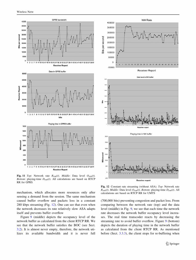
mechanism, which allocates more resources only after

sensing a demand from the session. The same mechanism

caused buffer overflow and packets loss in a constant

280 kbps streaming (Fig. 12). One can see that even when

the network decreases its rate relatively slow ASA adapts

itself and prevents buffer overflow

Figure 9 (middle) depicts the occupancy level of the

network buffer as calculated from the client RTCP RR. We

see that the network buffer satisfies the BOC (see Sect.

3.2). It is almost never empty, therefore, the network uti-

lizes its available bandwidth and it is never full

(700,000 bits) preventing congestion and packet loss. From

comparing between the network rate (top) and the data

level (middle) in Fig. 9, we see that each time the network

rate decreases the network buffer occupancy level increa-

ses. The real time transcoder reacts by decreasing the

streaming rate to avoid buffer overflow. Figure 9 (bottom)

depicts the duration of playing time in the network buffer

as calculated from the client RTCP RR. As mentioned

before (Sect. 3.3.3), the client stops for re-buffering when

Fig. 11 Top: Network rate RNW(t). Middle: Data level ONW(t).Bottom: playing-time DNW(t). All calculations are based on RTCP

RR for GPRS

Fig. 12 Constant rate streaming (without ASA). Top: Network rate

RNW(t). Middle: Data level ONW(t). Bottom: playing-time DNW(t). All

calculations are based on RTCP RR for UMTS

Wireless Netw

123

the playing time duration in its buffer reaches 0. The sum

of playing time in the client and network buffers is con-

stant; therefore, more playing time in the network buffer

means less playing time in the client buffer. The longest

playing time recorded in the network buffer during the test

session was 940 ms. It means that up to 940 ms were

reduced from the cellular client buffer. The initial buffering

time in cellular clients is usually 3–5 s; therefore, during

the test session there was always enough time in the cel-

lular client buffer to play continuously.

Figures 10 and 11 depict the network rate, the network

buffer data and playing time levels during a test session on

EDGE and GPRS, respectively. The initial bit rates were

30 kbps for GPRS and 65 kbps for EDGE. We can see that

the BOC was always satisfied: the network was fully uti-

lized without causing buffer overflow and packet loss.

Figure 12 depicts streaming without using any rate

control. The streaming rate is constantly 280 kbps. At

the first 10 s of the session the network rate is low

(RNWðtÞ � 200 kbps). However, the streaming server that

does not use rate control, continues to send RS(t) =

280 kbps. The extra bits are accumulated in the network

buffer and reach the maximal level of 700,000 bits, which

is the maximal size of the network buffer. Thus, remaining

bits are discarded. In the first 11 s, 105 from 284 packets

were lost which results in an un-usable video. We see that

the network buffer playing time reached 2,500 ms.

Therefore, the client buffer is missing 2,500 ms. The initial

buffering time is 3,000 ms and the client buffer did not

stop for re-buffering. This happens because the network

buffer was filled before the client buffer emptied and we

see packet loss instead of client re-buffering.

5.2 Simulation results

The streaming sever, network and client model as was

described in Sect. 3.1, was implemented in Matlab. We use

ASA to set the streaming server streaming rate. The net-

work rate is determined according to Poisson distribution

with average rate k (see Eq. 3). The simulation parameters

are given in Table 1.

Figure 13 depicts the ASA simulation results. At the top

right we see the average available rate and the actual

streaming/encoding rate. During the first 30 s, the available

network rate is 80,000 bps and during the next 30 s

40,000 bps. At the top left we see the network rate RNW(t)

which follows the available network rate even when it

drops in half (at 30 s). The streaming server response is

influenced also by the network and client buffers occu-

pancy levels in data size and playing time. At the middle

left we see the data level in the NW buffer ONW(t) and

client buffer. The BOC is almost always satisfied in the

network buffer because it is almost never empty and never

full. Therefore, the calculated usage percentage of the

network is 99%. The network buffer data level is constantly

around DONW = 60,000 bits and the maximal data level

reached 120,000 bits. We can also see the data level in the

client buffer (in red which means that there is always data

in the player buffer to continuously play the video and it

never reaches high levels to cause buffer overflow. The

histogram of the data level ONW(t) in the NW buffer is

given in the bottom left. We see that it resembles a

Gaussian around DONW = 60,000 bits as predicted in the

analysis (Sect. 4). At the middle right we see the playing-

time in the NW buffer DNW(t) and client buffer DC(t). The

BOC is always satisfied. Therefore, the client never stop-

ped for re-buffering.

Figure 14 depicts streaming without rate control at a

constant rate RS(t) = 60,000 bps. At the top right we see

the average available rate and the actual streaming/

encoding rate. During the first 30 s the available network

rate is 80,000 bps and during the next 30 s 40,000 bps. At

the top left we see the network rate RNW(t). During the first

30 s, the average available rate is 80,000 bps but the net-

work used only 60,000 bps because this is the rate the

streaming server used. (see top right: streaming rate RS(t)).

During the next 30 s, the average network rate is

40,000 bps. However, the streaming server that does not

use rate control, continues to send RS(t) = 60,000 bps. The

extra bits accumulate in the network buffer (bottom left).

During the first 30 s, the network buffer is mostly empty

and the network rate is under-used. During the next 30 s,

the network buffer is filling, and in real network will

overflow. At the bottom right we see the playing-time in

the NW buffer DNW(t) and client buffer DC(t). During the

last 30 s, the playing-time in the client buffer DC(t) = 0.

Therefore, the client does not have media to play and has to

stop for re-buffering.

6 Conclusion and future work

We introduce in this work the ASA algorithm for adap-

tive streaming of video over cellular networks. The ASA

Table 1 Simulation parameters

Parameter Value

RR period 1 s

Initial buffering 3 s

Initial streaming rate 70 kbps

FPS 15

Frames per packet 1

Wireless Netw

123

uses the standard RTSP and RTP protocols and can work

with any 3GPP standard client. The algorithm satisfies

the BOC condition that enables an optimal utilization of

the network resources without degrading the video

quality. The BOC is satisfied when the streaming-server,

network and client buffers stay in a partially full state,

never empty and never full, thus, enabling a pause-less

streaming without causing congestion and packet loss.

The ASA supports separation between the streaming rate

and the encoding rate, enabling a better utilization of the

network resources. It also enables features like scalable

video (a limited number of encoding rates) and fast

start (reducing the initial client buffering time by

compromising the initial quality). We tested the ASA on

UMTS, EDGE and GPRS networks and found out that

the BOC was almost always satisfied.

The ASA can generate a more steady encoding rate by

filtering the data from the RTCP receiver reports and by

putting some limitation on the streaming and encoding rate

change. Furthermore, an automatic configuration of the

ASA parameters (current and future) for a given network

can simplify its use. Another topic for future work is

improving the friendliness of the ASA to TCP streams.

Some state-of-the-art algorithms like TFRC pay attention

to this issue. It seems that currently most of the video

streaming users in the mobile networks do not combine

0 2 4 6 8 10 12 14

x 104

0

200

400

600

800

1000

1200

1400

Bits

Occ

urre

nce

Histogram of the Data level in the client buffer

0 1 2 3 4 5 6 7x 10

4

0

0.5

1

1.5

2

2.5

3

3.5x 10

5

milisecond

bit

Data level in client buffer (Red), Data level in NW buffer (Green)

0 1 2 3 4 5 6x 10

4

0

0.2

0.4

0.6

0.8

1

1.2

1.4

1.6

1.8

2x 10

5

milisecond

bit p

er s

econ

d

NW rate

0 1 2 3 4 5 6 x 104

0

0.2

0.4

0.6

0.8

1

1.2

1.4

1.6

1.8

2x 10

5

milisecond

bit p

er s

econ

d

Streaming rate (Red), Average NW rate (Green)

0 1 2 3 4 5 6 7x 10

4

0

500

1000

1500

2000

2500

3000

3500

milisecond

mili

seco

nd

Playing time in client buffer (Red), Playing time in NW buffer (Green)

Fig. 13 ASA simulation. Topleft: Network rate RNW(t); Topright: streaming/encoding rate

RS(t) = RSE(t); Middle left: data

level in the NW buffer ONW(t)and in client buffer; Middleright: playing-time in the NW

buffer DNW(t) and in client

buffer DC(t); Bottom left:Histogram of the data level in

the NW buffer ONW(t)

Wireless Netw

123

TCP and UDP streams. Moreover, most of the mobile

clients do not allow combining streams unless the mobile

client is used as a modem for a computer.

References

1. 3GPP, TSGS-SA, Transparent end-to-end Packet Switched

Streaming Service (PSS). Protocols and codecs (Release 6), TS

26.234, v. 6.3.0, 03-2005.

2. 3GPP, TSG-SA, Transparent end-to-end Packet Switched

Streaming Service (PSS). RTP usage model (Release 6), TR

26.937, v. 6.0.0, 03-2004.

3. Kleinrock, L. (1976). Queueing systems Volume 2: Computerapplications. John Wiley & Sons, Inc.

4. IETF, RTP: A Transport Protocol for Real-Time Applications,

RFC 3550, July 2003.

5. Curcio, I. D. D., & Leon, D. (2005). Application rate adaptation

for mobile streaming. IEEE Int. Symp. on a World of Wireless,Mobile and Multimedia Networks (WoWMoM ’05). Taormina/

Giardini-Naxos (Italy), 13–16, June 2005.

6. Curcio, I. D. D., & Leon, D. (2005). Evolution of 3GPP streaming

for improving QoS over mobile networks. IEEE InternationalConference on Image Processing. Genova, Italy, 2005.

7. Schierl, T., Wiegand, T., & Kampmann, M. (2005). 3GPP com-

pliant adaptive wireless video streaming using H.264/AVC, ICIP

2005. IEEE International Conference on Image Processing, Vol.

3, no. 11–14, pp. III-696–III-699, Sept. 2005.

8. Floyd, S., Handley, M., Padhye, J., & Widmer, J. (2000). Equa-

tion-based congestion control for unicast applications. In Pro-ceedings of the ACM SIGCOMM 2000, pp. 43–56, August 2000.

9. Floyd, S., & Fall, K. (1999). Promoting the use of end-to-end

congestion control in the internet. IEEE/ACM Transactions onNetworking, 7(4), 458-472.

10. Chen, M., & Zachor, A. (2004). Rate control for streaming video

over wireless. In Proceedings of the IEEE INFOCOM, Hong

Kong, China, pp. 1181–1190, 2004.

11. Alexiou, A., Antonellis, D., & Bouras, C. (2007). Adaptive and

reliable video transmission over UMTS for enhanced perfor-

mance. International Journal of Communication Systems, 20(12),

1315–1335

12. Koenen, R. (2002). MPEG-4 Overview—V.21—Jeju Version,

ISO/IEC JTC1/SC29/WG11 N4668, March 2002.

13. Farber, N., & Girod, B. (1997). Robust H.263 compatible video

transmission for mobile access to video servers. In Proc. IEEEInternational Conference on Image Processing (ICIP-97), Santa

Barbara, CA, USA, Vol. 2, pp. 73–76, October 1997.

14. Joint Video Team of ITU-T and ISO/IEC JTC 1, Draft ITU-T

Recommendation and Final Draft International Standard of Joint

Video Specification (ITU-T Rec. H.264—ISO/IEC 14496-10

AVC), document JVT-G050r1, May 2003; technical corrigendum

1 documents JVT-K050r1 (non-integrated form) and JVT-K051r1

(integrated form), March 2004; and Fidelity Range Extensions

documents JVT-L047 (non-integrated form) and JVT-L050

(integrated form), July 2004.

15. Schierl, T., Kampmann, M., & Wiegand, T. (2005). H.264/AVC

interleaving for 3G wireless video streaming, ICME 2005. IEEEInternational Conference on Multimedia and Expo, no. 4, pp.

6–8, July 2005.

0 1 2 3 4 5 6 7 8x 10

4

0

1

2

3

4

5

6

7

8 x 105

milisecond

bit

Data level in client buffer (Red), Data level in NW buffer (Green)

0 1 2 3 4 5 6 7 8x 10

4

0

0.2

0.4

0.6

0.8

1

1.2

1.4

1.6

1.8

2x 10

5

milisecond

bit p

er s

econ

d

NW rate

0 1 2 3 4 5 6 7 8x 10

4

0

0.2

0.4

0.6

0.8

1

1.2

1.4

1.6

1.8

2x 10

5

milisecond

bit p

er s

econ

d

Streaming rate (Red), Average NW rate (Green)

0 1 2 3 4 5 6 7 8x 10

4

0

2000

4000

6000

8000

10000

12000

14000

milisecondm

ilise

cond

Playing time in client buffer (Red), Playing time in NW buffer (Green)

Fig. 14 Simulation of constant

streaming rate. Top left:Network rate RNW(t); Top right:streaming/encoding rate

RS(t) = RSE(t); Bottom left: data

level in the NW bufferONW(t)and client buffer; Bottom right:playing-time in the NW buffer

DNW(t) and client buffer DC(t)

Wireless Netw

123

16. Skellam, J. G. (1946). The frequency distribution of the differ-

ence between two Poisson variates belonging to different popu-

lations. Journal of the Royal Statistical Society: Series A, 109(3),

296.

17. IETF, Real Time Streaming Protocol (RTSP), RFC 2326, April

1998.

Author Biographies

Y. Falik is the CTO of RTC

Ltd. which specializes in Image/

Video processing and computer

vision. He specializes in video/

image compression and video

streaming. Prior to RTC he

managed algorithms groups in

Adamind (2005–2007) and

Emblaze (2000–2005). Previ-

ously, he developed innovative

PowerPC chip that runs on

compressed code in Motorola

(1997–2000), and worked for a

scientific group in the Israeli

army (1993–1996). He holds an

M.Sc in computer science from the Tel-Aviv University.

A. Averbuch was born in Tel

Aviv, Israel. He received the

B.Sc and M.Sc degrees in

Mathematics from the Hebrew

University in Jerusalem, Israel

in 1971 and 1975, respectively.

He received the Ph.D degree in

Computer Science from

Columbia University, New

York, in 1983. During 1966–

1970 and 1973–1976 he served

in the Israeli Defense Forces. In

1976–1986 he was a Research

Staff Member at IBM T.J.

Watson Research Center, York-

town Heights, in NY, Department of Computer Science. In 1987, he

joined the School of Computer Science, Tel Aviv University, where

he is now Professor of Computer Science. His research interests

include applied harmonic analysis, wavelets, signal/image processing,

numerical computation and scientific computing (fast algorithms).

U. Yechiali is professor emeri-

tus from the operations research

and statistics in the Department

of Statistics and Operations

Research (chair the department

twice), School of Mathematical

Sciences, Tel Aviv University,

Israel. His major research fields

are: Queueing theory and its

applications, performance eval-

uation, telecommunications,

reliability, operations research

modeling, applied probability.

He got his B.Sc. (cum laude) in

Industrial and Management

Engineering, Technion, Haifa, Israel in 1964, M.Sc. in Operations

Research, Technion, Haifa, Israel in 1966 and his Dr. Eng. Sci. in

Operations Research, Columbia University, New York, USA in 1969.

He had visiting professorship in New York University, Columbia

niversity. He got in 2004 the ORSIS Award for ‘‘Life Achievement’’

in Operations Research. He was an Associate Editor, Probability in

the Engineering & Informational Sciences, Member of Editorial

Board, European Journal of Operational Research and Board of

Editors, Advances in Performance Analysis.

Wireless Netw

123