transmission algorithm for video streaming over cellular
TRANSCRIPT

Transmission algorithm for video streaming over cellular
networks
Y. Falik1, A. Averbuch1, U. Yechiali2
1School of Computer Science, Tel Aviv University
Tel Aviv 69978, Israel
2Department of Statistics and Operations Research
School of Mathematical Sciences, Tel Aviv University
Tel Aviv 69978, Israel
February 14, 2007
Abstract
2.5G and 3G cellular networks are becoming more and more widespread. Therefore,
the need for value added services is increasing rapidly. One of the key services that op-
erators seek to provide is streaming of rich multimedia content. However, the network
characteristics are making the use of streaming applications very difficult with an unac-
ceptable QoS.
The 3GPP standardization body has standardized streaming services. A standard
solution for multimedia streaming will benefit operators and users. There is a demand for
a mechanism that will enable a good quality multimedia streaming using 3GPP standard.
This paper describes an adaptive streaming algorithm using 3GPP standard that im-
proves significantly the quality of service in varying network conditions and monitors its
performance using queueing methodologies. The algorithm utilizes the available buffers
on the way of the streaming data in a unique way that guarantees high QoS. The system
is analytically modeled: the streaming server, the cellular network and the cellular client
are modeled as cascaded buffers and the data is passed between them sequentially. The
proposed algorithm controls these buffers’ occupancy levels by controlling the transmis-
sion and the encoding rates of the streaming server to achieve high QoS for the streaming.

Adaptive streaming algorithm (ASA) is the proposed algorithm. It overcomes the inher-
ent fluctuations in the bandwidth of the network. The algorithm was tested on General
Packet Radio Service (GPRS), Enhanced Data rates for GSM Evolution (EDGE), Univer-
sal Mobile Telecommunication System(UMTS) and CDMA1X networks and the results
showed substantial improvements over other standard streaming methods used today.
1 Introduction
Streaming video is becoming a common application on 2.5 and 3rd generation cellular networks.
The need for value added services on cellular networks is growing rapidly and thus 3GPP -
the 3rd Generation Partnership Project - that defines the standard for 3rd generation cellular
networks dedicated a special work group for streaming video [1, 2]. The problem is that the low
and fluctuated bandwidth of the network is making the use of streaming applications – while
maintaining steady and smooth stream with high Quality of Service (QoS)– very difficult.
There are several reasons for bandwidth fluctuations:
Network load. In each cell, the channel resources are divided between voice and data sessions.
The result is that every few seconds the amount of channel resources allocated to a
streaming session is changed and there is no guarantee for steady constant bit allocation.
Radio network conditions. The network has a bounded retransmission mechanism, which
resends a packet whenever a client fails to receive it. This results in fluctuation of the
available bandwidth whenever the radio conditions change while causing congestions and
delays.
Available bandwidth. Finding out the network bandwidth is a problem. There is no stan-
dard way to acquire the bandwidth information from the network so one has to rely on
reports from the client that have an unknown delay. The client reports only on an integer
number of packets that were received. Usually, to avoid packetization overhead, the size
of the packet is very large, so one packet may be received after up to 2 seconds. Thus,
the bandwidth can be measured only in large discrete steps with coarse resolution.
These problems cause the operator to utilize only a fraction of its bandwidth on the one
hand, and cause the end user to experience a poor video quality on the other hand.
Figure 1 illustrates the UMTS network architecture. The streaming server resides either
in the Internet (PDN in Fig. 1) or usually in the operator premises just before the GGSN
2
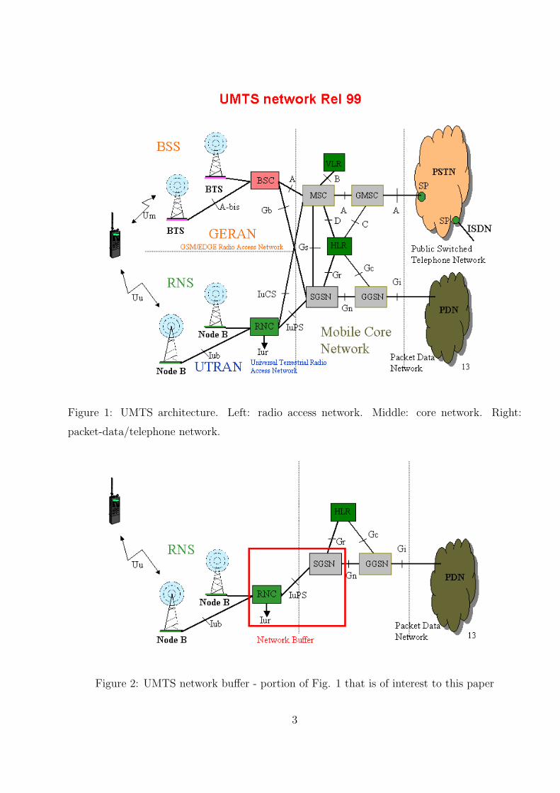
Figure 1: UMTS architecture. Left: radio access network. Middle: core network. Right:
packet-data/telephone network.
Figure 2: UMTS network buffer - portion of Fig. 1 that is of interest to this paper
3

(Gateway GPRS Support Node) which acts as a gateway between the UMTS wireless data
network and other networks such as the Internet or private networks. The data is passed from
the GGSN to the SGSN (Serving GPRS Support Node) which does the full set of inter-working
with the connected radio network and then to the RNC (Radio Network Controller), which is
the governing element in the UMTS radio access network (UTRAN), responsible for control of
the Node-Bs (base stations) that are connected to the controller. The RNC carries out radio
resource management, some of the mobility management functions and is the point where
encryption is done before user data is sent to and from the mobile.
The data is stored in the network before transmission in the SGSN and RNC to enable han-
dovers and retransmissions (see Fig. 2). These buffers are reallocated for each data session. In
this paper, these buffers are considered as a single buffer (“The Network buffer”). Although the
streaming server does not control the network buffer directly, its behavior during the streaming
session is critical in assuring a smooth data stream and good QoS.
In order to enable a good quality and smooth multimedia streaming there is a need for
adaptive streaming. The use of constant bit rate media as it comes from the encoder on a
varying bit rate channels is not recommended.
The term adaptive here means that a streaming service is given the feature that enables
to adapt to varying network conditions. Examples of such variations include variations of
throughput, delay, and intra/inter-operator roaming to networks with or without QoS support.
These situations are not very critical for non-real time traffic such as downloading, ftp,
browsing. However, they become critical for continuous media transmission, such as streaming,
where the user experience drops if the service loses its inherent properties of continuity and syn-
chronization. For instance, continuous (or pause-less) playback is the number one requirement
for a successful streaming service. When the network throughput is constantly varying during
a session, the effect on the end user’s client is that of picture freezes, pauses in the audio/video
playback, continuous rebufferings (i.e., re-loading from the streaming server a sufficient amount
of media data to be streamed with no interruptions) and bad media quality (caused by packet
losses derived by network buffers overflow).
Adaptive streaming avoids the above phenomena and ensures pause-less playback to the end
user, yielding a superior user experience compared to conventional streaming. The streaming
server uses adaptive streaming by changing the media rate and the streaming rate. Media rate
means the bit rate in which the media is played (e.g. 32 kbps video means that each second of
the compressed video is described by 32kb). The media rate can be changed in live encoding by
4

changing the encoding bit rate, or offline by keeping a set of media streams of the same content
encoded at different bit rates and performing seamless switching between the different media
streams. For example, if a streaming session starts at 64 kbps with good network throughput,
and subsequently the network throughput halves, the streaming server can switch to a lower bit
rate stream (e.g., 32 kbps) to guarantee pause-less playback and avoid network buffers overflow
that would cause packet losses and bad QoS. The server can switch up to the 64 kbps media
stream when the network conditions improve.
Figure 3: Multimedia streaming that is modeled: functional entities
The proposed adaptive media streaming performance is analyzed using methods from queue-
ing theory. It is commonly used to analyze communication networks. Queuing models are
frequently modeled as Poisson processes through the use of the exponential distribution.
For the analysis of the system, the data flow in a streaming session (Fig. 3) is modeled as
having one input process (the streaming server) and two serially connected queues - the mobile
network buffer and the client buffer. The data is delivered from the streaming server to the
network, where it is queued (network buffer) and served (transmitted), arriving at the client
where it is queued (client jitter buffer) and served (played).
The data flow from the streaming server is controlled. The mobile network buffer queue
serves (transmits) the data in a rate that is modeled as a Poisson process. The client queue
(Fig. 3) serves (plays) the data in the bit rate at which it was encoded. The control mechanism
of the streaming server and the performance analysis of the mobile network and client queues
are the subject of this paper.
The physical implementation of the model is illustrated in Fig. 2. The streaming server
resides in the PDN, the network buffer is in the SGSN and RNC and the client buffer is in the
5

client.
1.1 Motivation
The current income of the cellular operators from voice calls is saturated. To increase the
average revenue per user (ARPU) the operators need value added services which is a telecom-
munications industry term for non-core services or, in short, all services beyond standard voice
calls. Value-added services add value to the standard service offering, spurring the subscriber
to use their phone more and allowing the operator to drive up their ARPU. One of the most
promising services is the transmission of rich multimedia content, which is why most of the
cell phones manufactured nowadays, have multimedia capabilities. Currently, the poor video
quality on the low and fluctuated bandwidth networks is a problem that prevents the operators
from charging for video services.
1.2 Contribution and results
This paper introduces a model for maintaining a steady QoS performance for a server-network-
client streaming as described schematically in Fig. 3. An algorithm that is best-fit for this
problem model is suggested. The ‘best-fit’ of the algorithm means that all the available band-
width of the streaming session is utilized and no delays and packet loss are caused. The
algorithm can be used on any 3GPP standard client that sends RTCP reports [3].
Moreover, the new model offers new ways for streaming which enables to allocate more bits
to more complex scenes (similarly to 2-pass encoding techniques), thus enabling better video
quality.
The algorithm also enables a fast start and zero-ending, which means that the video stream
starts with very low buffering delay and ends with better video quality.
This algorithm was tested on GPRS, EDGE, UMTS and CDMA-1X networks. The re-
sults showed substantial improvements over other standard methods for streaming media in
use today. The streaming session bandwidth was fully utilized, which enhanced the video qual-
ity. The algorithm was also tested in extreme network conditions (in a network manufacturer
laboratory), showing good results.
The structure of the paper is as follows. In section 2, we present related work. In section 3,
we describe an adaptive streaming algorithm to be used in the streaming server to achieve better
QoS. The performance of the algorithm, using methods from queueing theory, is described in
6

section 4. Experimental and simulation results on several cellular networks are presented in
section 5.
2 Related work
2.1 Congestion control
In cellular networks, the low and fluctuated bandwidth is making use of streaming applications
– while maintaining steady and smooth stream with high Quality of Service (QoS) – very
difficult. Congestion control is aimed at solving this problem by adapting the streaming rate
to the network conditions.
The solution standardized in 3GPP Release 6 for adaptive streaming is described in [9, 10].
The 3GPP PSS specifications introduce signaling from the client to the server, which allows
the server to have the information it needs in order to best choose both transmission rate and
media encoding rate at any time.
The rate adaptation problem is termed curve control. The playout curve shows the cumu-
lative amount of data the decoder has processed by a given time from the client buffer. The
encoding curve indicates the progress of data generation if the media encoder runs in real-time.
The transmission curve shows the cumulative amount of data sent out by the server at a given
time. The reception curve shows the cumulative amount of data received in the client buffer at
a given time.
The distance between the transmission and reception curves corresponds to the amount of
data in the network buffer and the distance between the reception and playout curves corre-
sponds to the amount of data in the client buffer. Curve control here means constraining by
some limits the distance between two curves (e.g., by a maximum amount of data, or maximum
delay). This problem is equivalent to controlling the network and the client buffers. However,
there is no specific suggestion for choosing the transmission rate and media encoding rate, and
there is no treatment for client that do not support 3GPP Release 6 signaling.
A widely popular rate control scheme over wired networks is equation-based rate control
([5, 6]), also known as TCP friendly rate control (TFRC). There are basically three main
advantages for rate control using TFRC: first, it does not cause network instability, which
means that congestion collapse is avoided. More specifically, TFRC mechanism monitors the
status of the network and every time that congestion is detected, it adjusts the sending rates of
7

the streaming applications. Second, it is fair to TCP flows, which are the dominant source of
traffic on the Internet. Third, the TFRC’s rate fluctuation is lower than TCP, making it more
appropriate for streaming applications which require constant video quality.
A widely popular model for TFRC is described by
T =kS
RTT√
p
where T is the sending rate, S is the packet size, RTT is the end-to-end round trip time, p is
the end-to-end packet loss rate, and k is a constant factor between 0.7 and 1.3, depending on
the particular derivation of the TFRC equation.
The use of TFRC for streaming video over wireless networks is described in [7]. It resolves
two TFRC difficulties: first, TFRC assumes that packet loss in wired networks is primarily due
to congestion, and as such it is not applicable to wireless networks in which the bulk of packet
loss is due to error at the physical layer. Second, TFRC does not fully utilize the network
channel. It resolves it by multiple TFRC connections that results in full utilization of the
network channel. However, it is not possible to use multiple connections in standard 3GPP
streaming clients.
The use of TFRC for streaming video over UMTS is given in [8]. The round trip time and
the packet loss rate are estimated using standard real time control protocol (RTCP) RR. The
problem of under utilization of one TFRC connection remains.
2.2 Video scalability
Adaptive streaming enables to achieve a better QoS compared to conventional streaming. The
streaming server uses adaptive streaming by changing the media rate and the streaming rate.
Media rate means the bit rate in which the media is encoded/played. The media rate can be
changed in live encoding by changing the encoding bit rate or offline. Several approaches were
suggested to enable dynamic bit rate change:
MPEG-4 ([11]) simple scalable profile is an MPEG-4 tool which enables to change the
number of frames per second or the spatial resolution of the media. It encodes the media in
several dependent layers and determines the media quality by addition or subtraction of layers.
MPEG-4 FGS (Fine granularity scalability) is a type of scalability where an enhancement
layer can be truncated into any number of bits that provides a corresponding quality enhance-
ment.
8
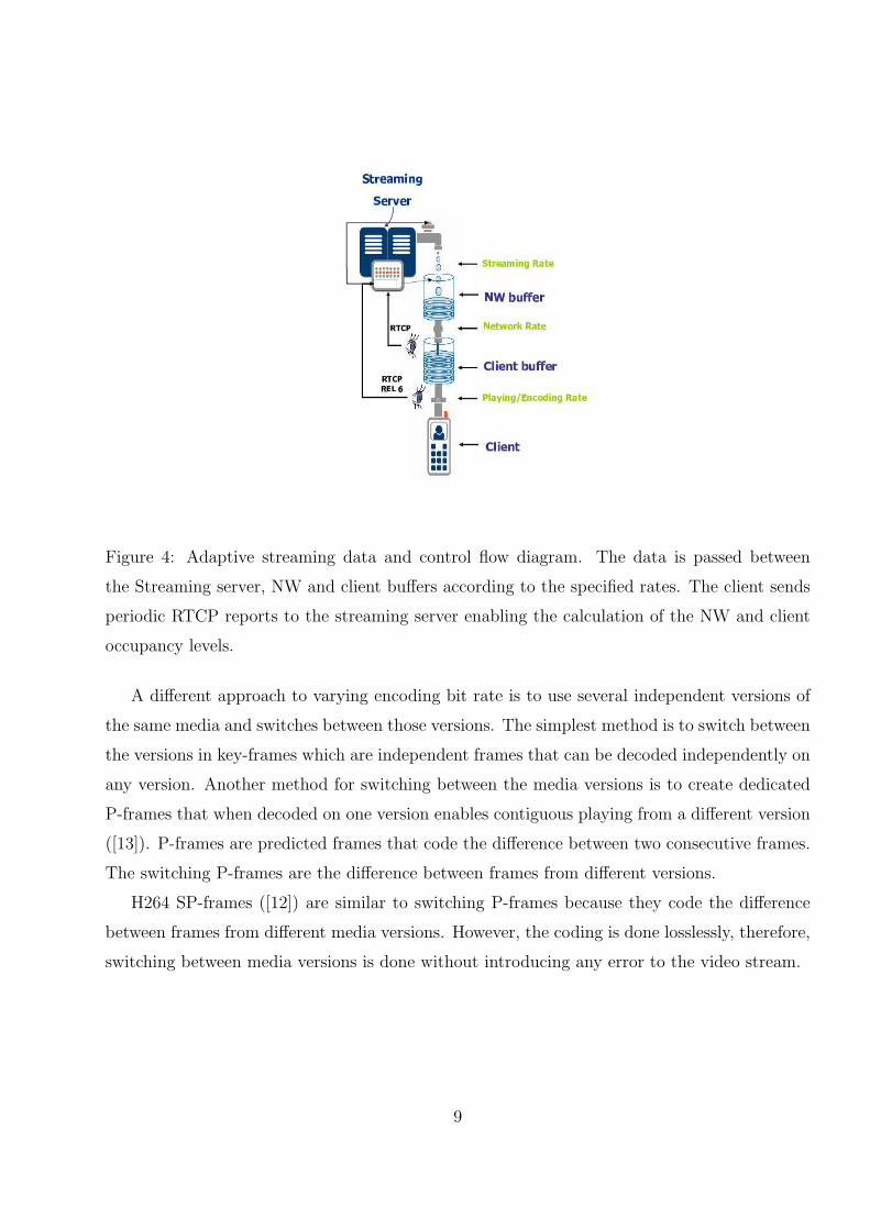
Figure 4: Adaptive streaming data and control flow diagram. The data is passed between
the Streaming server, NW and client buffers according to the specified rates. The client sends
periodic RTCP reports to the streaming server enabling the calculation of the NW and client
occupancy levels.
A different approach to varying encoding bit rate is to use several independent versions of
the same media and switches between those versions. The simplest method is to switch between
the versions in key-frames which are independent frames that can be decoded independently on
any version. Another method for switching between the media versions is to create dedicated
P-frames that when decoded on one version enables contiguous playing from a different version
([13]). P-frames are predicted frames that code the difference between two consecutive frames.
The switching P-frames are the difference between frames from different versions.
H264 SP-frames ([12]) are similar to switching P-frames because they code the difference
between frames from different media versions. However, the coding is done losslessly, therefore,
switching between media versions is done without introducing any error to the video stream.
9

3 Adaptive Streaming Algorithm (ASA)
This section describes the proposed Adaptive Streaming Algorithm (ASA) to be used in the
streaming server. A general description of the system is given in Fig. 4. The streaming server
controls two transmission parameters - the streaming rate and the encoding rate.
In conventional streaming servers, these two rates are equal to each other, which means
that the video clip is streamed at the same rate as it was encoded. The equality of the rate
imposes an unnecessary restriction on the system, which causes sub-optimal utilization of the
network resources. In the proposed algorithm, this restriction is removed, thus enabling a full
utilization by flexible adaptation to the network resources.
The system is modeled in the following way: the streaming server, the cellular network and
the cellular client are modeled as cascaded buffers (see Fig. 4), and the data is passed between
them sequentially. The goal of the algorithm is to control all these buffers-occupancy levels by
controlling the transmission rate of the streaming server and the decoding rate of the cellular
client to achieve streaming with high QoS.
3.1 Data Flow and Buffers
In the ASA model, all the functional entities of the multimedia streaming are considered as
buffers (see Fig. 4). Three buffers are used:
Streaming server buffer: In an on-demand scenario, the streaming server can use the video
file as a buffer and stream the file faster or slower than the video rate. In a live scenario,
the server can delay the video for several seconds and use this data as a buffer. The
streaming server controls both the encoding rate of the transmitted media and the data
transmission rate, and so each transmitted packet has two different size parameters - its
size in bits and its duration in media playing time.
Network buffer: The network is comprised of several components and network-layers and
each component/layer uses a buffer. All these components are connected by a LAN,
which is much faster than the rate of the cellular network and thus all these components
can be virtually modeled as a single buffer. The input of this buffer is the output of the
streaming server. Its output is the data sent over the mobile network to the client. Its
rate is determined by the network conditions and is assumed to be a Poisson process.
10

The mobile network buffer has two parameters - its size in bits (occupancy level) and its
size in media playing time.
Client buffer: The client uses a jitter buffer, which holds the data sent from the network
before playing it. Its input is the data received from the network and its output is the
media played at the rate it was encoded in. Again, its size can be measured both in bits
or in playing time.
3.2 Buffer Occupancy Condition
ASA is designed to assure that during the entire session each buffer stays in a partially
full state, never empty and never full. This condition will be referred to as the Buffer
Occupancy Condition (BOC).
We claim that the BOC enables an optimal utilization of the network resources without
degrading the video quality. The reasons are: on one hand, when the network buffer is empty,
the network is idle and wastes potential transmission time. On the other hand, when the
network buffer is full, packet loss occurs, because the network buffer denies the entering packets.
When the client buffer is empty, the player has to stop the video clip for re-buffering. When
the client buffer is full, packet loss occurs, because the client buffer denies the entering packets.
The conventional streaming servers do not satisfy the BOC condition and usually there are
periods that the network is idle.
To apply the BOC, we have to know the bandwidth and occupancy of the mobile network.
There is no standard way to query the status of the network and client buffers. The only
available information is the standard RTCP report from the client to the server. In the RTCP
report, the client periodically reports to the server the ID of the last packet that was received.
This information can now be used by the server to estimate the occupancy of the network buffer
and the network data transfer rate. In 3GPP rel. 6, the RTCP receiver reports include also the
ID of the last packet that was played in the client. When this standard will be implemented
in the new cellular phones, it will enable the server to calculate accurately the client buffer
occupancy.
In case the cellular phone does not support 3GPP rel. 6, ASA estimates the client buffer
occupancy (section 3.3.3).
11

3.3 ASA description
The description of ASA is divided into three sections:
Section 3.3.1 describes the way ASA controls the network buffer occupancy level by changing
the streaming rate.
Section 3.3.2 describes the way ASA controls the client buffer occupancy level by changing
the encoding rate and by controlling the network buffer occupancy level. The control is
based on 3GPP Rel. 6 information.
Section 3.3.3 describes the way ASA controls the client buffer occupancy level based on the
occupancy estimation when 3GPP Rel. 6 information is unavailable.
Notation:
RNW (t) The cellular network incoming rate at instant t.
RS(t) The streaming server outgoing rate at instant t.
RES (t) The streaming server encoding rate at instant t which is also the client
outgoing rate after an unknown delay.
ONW (t) The occupancy level of the network buffer in bits at instant t.
DNW (t) The duration of playing time in the network buffer at instant t.
DONW The desired occupancy level of the network buffer in bits.
TADJ An adjustment period.
DC(t) The duration of playing time in the client buffer at instant t.
DDC The desired duration of playing time in the client buffer.
P SES (t) The ratio between the streaming and encoding rate at instant t.
DS(t) The duration of playing time in the streaming server buffer at instant t.
DS(t) 6= 0 when the streaming and encoding rate differ.
3.3.1 Network Buffer
In order to satisfy the BOC, we first try to maintain the network buffer filled with as little data
as possible without ever being actually empty. The reason for this will be clarified later. We
want to achieve a constant occupancy level. The occupancy level ONW (t) is affected by the
network input and output rates. The output rate RNW (t) is the network data transfer rate,
which is not controlled by our application. The input rate RS(t) is the streaming server rate,
12

Figure 5: ASA flow
13

which is fully controllable. It is important to note that the video encoding rate RES (t) does not
affect the occupancy level.
The flow of ASA is given in Fig. 5. The calculation of the streaming rate RS(t) at time t
(“streaming rate calculation” in Fig. 5) takes into account the previous network rate RNW (t−τ)
τ units of time before as a prediction for the next network rate RNW (t), and adds to it a factor
that should adjust the occupancy level ONW (t) to some predetermined desired occupancy level
DONW after some predetermined adjustment period TADJ . More formally, the streaming rate
is determined by:
RS(t) = RNW (t − τ) +DONW − ONW (t − τ)
TADJ
· τ. (1)
RS(t) is computed every time an RTCP receiver report is received by the streaming server.
The desired network occupancy level DONW and the adjustment-period TADJ are constants
of the algorithm that differ for different network types such as GPRS and UMTS. Their actual
values are empirically tuned.
The network rate RNW (t) and the network buffer occupancy level ONW (t) are measured
through reports from the client. We rely on standard RTCP receiver report that every 3GPP
standard client sends. From each RTCP receiver report, the server calculates these parameters
and prescribes the streaming-rate RS(t) accordingly. This streaming-rate should adaptively
keep the network-buffer occupancyONW (t) close to the desired occupancy level DONW .
Example Assume the streaming session begins with a streaming rate of 10kbps while the
potential network rate is a constant 30kbps. The streaming server cannot know the potential
network rate, but since the network buffer will be empty after the first RTCP report, it will raise
the streaming rate, and data will start accumulating in the network buffer. Subsequently, the
network buffer will reach its desired occupancy level and then the streaming rate will decrease
until it will equate the network rate, and the network buffer will remain at the constant desired
occupancy level.
Throughout the session, a change in the network potential rate will only appear in the
actual network rate when the network buffer is neither empty nor full.
If the network rate increases, the occupancy level of the buffer decreases, and thus the
streaming rate will increase as a compensation until again the buffer will reach its desired
occupancy level and the two rates will equate.
Similarly, if the network rate decreases, the occupancy level of its buffer-occupancy increases,
14

and thus the streaming rate decreases as a compensation until again the buffer will reach its
desired occupancy level and the two rates will equate.
3.3.2 Client Buffer
The occupancy level of the client buffer is influenced by its input and output rates. The input
rate RNW (t) is the network transmission rate, which we have no control over. The output rate
RES (t) is the encoding rate, which is controllable. Therefore, in order to maintain the client
buffer in a partially-full state (satisfying BOC), we have to control the encoding rate.
The method that determines the encoding rate (“Encoding rate calculation” in Fig. 5) is
similar to the method used for determining the streaming rate, except that instead of the buffer
size in bits, we use the buffer size in playing time. Again, we set a desired occupancy level (in
playing time) and an adjustment-period. The playing time duration in a time unit is:
P SES (t) = 1 +
DDc − DC(t)
TADJ
.
P SES (t) is computed every time an RTCP receiver report is received in the streaming server.
The client plays the media at the same rate at which it is encoded, which accounts for the
‘1’ in the formula.
The actual encoding rate is
RES (t) =
RS(t)
P SES (t)
.
The control over the network buffer is direct. Any change in the streaming rate directly affects
the occupancy level. It differs from the control over the client buffer which is delayed. The
media data has to pass through the network buffer first. This delay might be crucial when the
network available bandwidth drastically decreases. In order to avoid this problem, we try to
maintain the network buffer filled with as little data as possible without ever being actually
empty.
The separation between the streaming and encoding rates is more important in the case
of scalable video. In that case, only a limited number of encoding rates are available. When
scalable video is used, ASA will choose the video level with encoding rate just below the
calculated encoding rate. The separation between the rates enables a smooth transmission
and a better utilization of the network although we have a limited number of encoding rates.
For example, the network rate RNW (t) average is 50kbps with jitter around the average. The
encoding rate RES (t) will remain 50 kbps. However, the streaming rate RS(t) will follow the
15

jittering network rate. In case the network rate drops the streaming rate will drop quickly
afterwords to prevent network buffer overflow. Then, the streaming rate will follow.
A real time transcoder with no internal buffer, will not be able to separate between the
streaming and encoding rates. Therefore, first the streaming rate RS(t) and then the encoding
rate RES (t) are calculated. The mutual streaming/encoding rate will be RS(t) = RE
S (t) =
Min(RS(t), RES (t)). Thus, network buffer overflow and client buffer underflow are prevented.
3.3.3 Client Buffer Occupancy Estimation
The client buffer occupancy level is reported in 3GPP rel. 6. The problem is that the majority
of the clients do not support rel. 6 and the client buffer occupancy level is unknown. Therefore,
we estimate its occupancy.
This estimate is based on the duration of playing time in each streaming server, network and
client buffers. The sum of playing time at the three buffers is DS(t)+DNW (t)+DC(t) = constant
during the streaming session (this is true as long as the client did not stop for re-buffering).
The above sum of playing time is constant because the media is entering the streaming server
at the encoding rate and leaving the client buffer at the encoding rate, as long as they both
did not stop playing. The sum of playing time is simply the time difference between the time
the streaming server started streaming and the time the client started playing.
The duration of playing time in the streaming server buffer DS(t) is the difference between
the playing time and the transmission time of the last sent packet. The duration of playing
time in the network buffer DNW (t) is the difference between the playing time stamps of the
last sent packet and the last received packet sent by the client RTCP report.
The duration of playing time in the client buffer DC(t) is not known but can be calculated
directly from the duration of playing time in the streaming server and the network buffer which
is known. Therefore,
DC(t) = constant − DS(t) − DNW (t). (2)
The constant in Eq. 2 is not known but its value is not so important because we only need
to monitor the change in the duration of playing time in the client buffer DC(t), and not its
absolute value.
16
4 Stochastic analysis of ASA performance
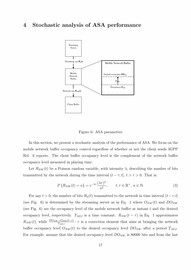
Figure 6: ASA parameters
In this section, we present a stochastic analysis of the performance of ASA. We focus on the
mobile network buffer occupancy control regardless of whether or not the client sends 3GPP
Rel. 6 reports. The client buffer occupancy level is the complement of the network buffer
occupancy level measured in playing time.
Let RNW (t) be a Poisson random variable, with intensity λ, describing the number of bits
transmitted by the network during the time interval (t − τ, t], t > τ > 0. That is:
P {RNW (t) = n} = e−λτ (λτ)n
n!, t, τ ∈ R
+, n ∈ N. (3)
For any t > 0, the number of bits RS(t) transmitted to the network in time interval (t− τ, t]
(see Fig. 6) is determined by the streaming server as in Eq. 1 where ONW (t) and DONW
(see Fig. 6) are the occupancy level of the mobile network buffer at instant t and the desired
occupancy level, respectively. TADJ is a time constant. RNW (t − τ) in Eq. 1 approximates
RNW (t), while DONW−ONW (t−τ)TADJ
· τ is a correction element that aims at bringing the network
buffer occupancy level ONW (t) to the desired occupancy level DONW after a period TADJ .
For example, assume that the desired occupancy level DONW is 80000 bits and from the last
17

RTCP receiver report (RR) we calculate that the network transmitted RNW (t − τ) = 50000
bits and the network occupancy level ONW (t) is 60000 bits. We also know that the RTCP RR
interval is τ = 1sec. In response, the streaming server adjusts the streaming rate RS(t) to be
RS(t) = 50000 + 80000−600002
· 1 = 60000bits, which is higher than the network rate. Therefore,
the occupancy level ONW (t) becomes close to the desired occupancy level DONW .
We now estimate Eq. 1 using Chebychev inequality (see section 4.1) and by Gaussian
approximation (see section 4.2).
4.1 Probability bounds on the ASA performance
Let ONW (t) be the occupancy of the network at a time when the process has reached its
stationary state, and let ONW (t − τ) be the occupancy of the network buffer one time step
earlier. We substitute Eq. 1 in Eq. 11 and get
ONW (t) ∼ ONW (t − τ) +DONW − ONW (t − τ)
TADJ
τ + RNW (t − τ) − RNW (t). (4)
By replacing the rates difference in Eq. 4 with the Skellam distribution and using TR , TADJ
τ,
we get
ONW (t) ∼ skellam(λτ) +DONW
TR
+TR − 1
TR
ONW (t − τ). (5)
When in stationary state, ONW (t) and ONW (t−τ) are identically distributed which means they
have the same expectation E{ONW (t)} = E{ONW (t − τ)} = µ and variance var{ONW (t)} =
var{ONW (t − τ)} = σ2 . We also know Skellam’s expectation to be 0 and variance to be 2λτ .
Taking expectation of both sides of Eq. 5 we write
E{ONW (t)} = E{skellam(λτ) +DONW
TR
+TR − 1
TR
ONW (t − τ)}. (6)
Using stationarity and substituting E{ONW (t)} = µ yields
µ = 0 +DONW
TR
+TR − 1
TR
µ. (7)
This implies that µ = DONW .
In the same way, we calculate the variance of ONW (t) according to Eq. 5 and get, assuming
independence between the variables,
var{ONW (t)} = var{skellam(λτ) +DONW
TR
+TR − 1
TR
ONW (t − τ)}. (8)
18

Substituting var{ONW (t)} = σ2 and assuming all RVs in Eq. 8 to be independent we have
σ2 = 2λτ + 0 +
(
TR − 1
TR
)2
σ2. (9)
From Eq. 9 we get σ2 =2λτT 2
R
2TR−1.
Actually, this result applies to any outgoing bit rate distribution. As long as it is memory-
less and its variance σ2NW is known, we have
σ2 =2σ2
NW T 2R
2TR − 1, µ = DONW .
After µ and σ are calculated, the probability for the occupancy level ONW (t) deviation from
the desired occupancy level DONW can be calculated by using Chebychev inequality
P {|ONW (t) − µ| ≥ aσ} ≤ 1
a2.
For example, in UMTS, DONW = 100000bits, σ2NW = λτ , τ = 1sec, λ = 350000bits and TR = 1.
The variance is σ2 = 2·350000·1·12
2·1−1= 700000 so that σ = 836.7. The probability for network buffer
underflow is P {|ONW (t) − 100000| ≥ 100000} ≤ 1119.52 . The UMTS buffer size is 600000 and
the probability for network buffer overflow is P {|ONW (t) − 600000| ≥ 600000} ≤ 1717.12 (since
σ = 836.7 and aσ = 600000). We see that even though Chebychev inequality is not considered
a “sharp” inequality it is sufficient for our purposes.
4.2 Analysis of ASA performance using Gaussian approximation
In this analysis, we assume that RNW (t− τ) in Eq. 1 is independent of ONW (t− τ). While this
is not accurate, it fits the spirit of the algorithm, as we are not using RNW (t− τ) because of its
value in the previous time step, but as an approximation to RNW (t) in the current time step.
To simplify the computations, we assume that the occupancy of the network buffer can be
negative.
The mobile network buffer can be analyzed as a Markov process ONW (t) : ONW (t) = i when
the network buffer is filled with i bits. The stationary distribution P i is the probability that
the process has value i in steady state. The transition probability Pi,j is the probability for
transition from ONW (t − τ) = i to ONW (t) = j. Formally,
P i,j = P {ONW (t) = j | ONW (t − τ) = i} . (10)
19

The occupancy level is the previous occupancy level plus the difference in the incoming and
outgoing data rates, i.e.
ONW (t) = ONW (t − τ) + RS(t) − RNW (t). (11)
Substituting Eq. 11 in Eq. 10 and get
Pi,j = P {ONW (t − τ) + [RS(t) − RNW (t)] = j | ONW (t − τ) = i} . (12)
Substituting Eq. 1 in Eq. 12 (while denoting TR∆= TADJ
τ) leads to
Pi,j = P{
ONW (t − τ) +[
DONW−ONW (t−τ)TR
+ RNW (t − τ) − RNW (t)]
= j | ONW (t − τ) = i}
= P{
i +[
DONW−iTR
+ RNW (t − τ) − RNW (t)]
= j | ONW (t − τ) = i}
.
Subtracting i + DONW−iTR
from both sides results in
Pi,j = P
{
[RNW (t − τ) − RNW (t)] = j − i − DONW − i
TR
| ONW (t − τ) = i
}
.
Since both RNW (t) and RNW (t − τ) are independent of ONW (t − τ) we get,
Pi,j = P
{
[RNW (t − τ) − RNW (t)] = j − i − DONW − i
TR
}
. (13)
In order to solve Eq. 13, we have to find the distribution of RNW (t−τ)−RNW (t). Assuming
that the network rate RNW (t) and its occupancy ONW (t) are independent, RNW (t−τ)−RNW (t)
is the difference between two i.i.d Poisson random variables with intensity λ. This difference
is called Skellam distribution [1], and can be approximated as Gaussian with expectation 0
and variance 2λτ . Since Gaussian is a continuous distribution, we analyze the occupancy as a
continuous variable. From now on, we denote by f(i) the density function of ONW (t) and by
f(i, j) the density function of the transition probability of ONW (t − τ) to ONW (t).
Denote by γµ,σ2 the density function of the Gaussian distribution γµ,σ2(x) = 1σ√
2πe
(x−µ)2
2σ2 ,
then
f(i, j) = γ0,2λτ
(
j − i − DONW − i
TR
)
=1√
4πλτe(j−i−
DONW −i
TR)2
4λτ . (14)
For the Markov chain, the stationary distribution and the transition probabilities satify the
balance equation
Pj =∞
∑
i=0
Pi · Pi,j,
∞∑
i=0
Pi = 1. (15)
20
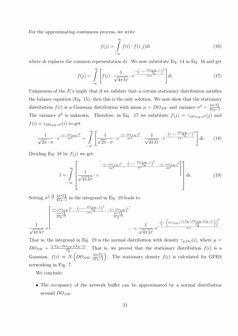
For the approximating continuous process, we write
f(j) =
∞∫
−∞
f(i) · f(i, j)di (16)
where di replaces the common representation dx. We now substitute Eq. 14 in Eq. 16 and get
f(j) =
∞∫
−∞
[
f(i) · 1√4πλτ
· e−(j−i−
DONW −i
TR)2
4λτ
]
di. (17)
Uniqueness of the Pi’s imply that if we validate that a certain stationary distribution satisfies
the balance equation (Eq. 15), then this is the only solution. We now show that the stationary
distribution f(i) is a Gaussian distribution with mean µ = DONW and variance σ2 =2λτT 2
R
2TR−1.
The variance σ2 is unknown. Therefore, in Eq. 17 we substitute f(j) = γDONW ,σ2(j) and
f(i) = γDONW ,σ2(i) to get
1√2π · σ
· e−(j−DONW )2
2σ2 =
∞∫
−∞
[
1√2π · σ
· e−(i−DONW )2
2σ2 · 1√4πλτ
· e−(j−i−
DONW −i
TR)2
4λτ
]
di. (18)
Dividing Eq. 18 by f(j) we get:
1 =
∞∫
−∞
1√4πλτ
· e
2664−(i−DONW )2
2σ2 +−(j−i−
DONW −i
TR)2
4λτ−
−(j−DONW )2
2σ2
3775
di. (19)
Setting σ2 ∆=
2λτT 2R
2TR−1in the integrand in Eq. 19 leads to
1√4πλτ
·e
26666664−(i−DONW )2
4λτT2R
2TR−1
+−(j−i−
DONW −i
TR)2
4λτ−
−(j−DONW )2
4λτT2R
2TR−1
37777775=
1√4πλτ
·e−
i−
DONW +
(j·TR−DONW )(TR−1)
T2R
!!2
4λτ .
That is, the integrand in Eq. 19 is the normal distribution with density γµ,2λτ (i), where µ =
DONW + (j·TR−DONW )(TR−1)
T 2R
. That is, we proved that the stationary distribution f(i) is a
Gaussian, f(i) ≈ N(
DONW ,2λτT 2
R
2TR−1
)
. The stationary density f(i) is calculated for GPRS
networking in Fig. 7.
We conclude:
• The occupancy of the network buffer can be approximated by a normal distribution
around DONW .
21

• TR is the ratio between the time TADJ it takes for the streaming server to correct the
occupancy and the sampling time τ . We are interested in values of TR that are greater
than 1. For these values, when TR grows, the variance grows as well.
• When TR = 12, the variance is infinite. It means that if the streaming server reacts too
fast. The system will constantly oscillate without reaching stationarity.
• By differentiating the variance2λτT 2
R
2TR−1with respect to TR we get ∂σ2
∂TR= 4λτTR(TR−1)
(2TR−1)2, and
we see that the variance is minimal when TR = 1.
Figure 7: Network buffer occupancy ONW (t) density function for GPRS. The x-axis is the
occupancy level of the network buffer in bits. We assume that the RTP packet size is 500
bytes, the desired occupancy level DONW is 14000 bytes, the average network rate λ is 15000
kbps and TR = 1.
5 Experimental and simulation results
5.1 Experimental results
The ASA was implemented on several commercial cellular networks providing good QoS. The
architecture is comprised of a streaming server, a real time transcoder and a cellular client (see
Fig. 8). The streaming server is located in the Internet and the transcoder is located between
22

Internet
Streaming server Transcoder implementing ASA
Cellular network Cellular client
Figure 8: Architecture for the experimental setup: A real time transcoder using ASA is located
between a streaming server and a cellular client.
the streaming server and the cellular client. The streaming server and the real time transcoder
used RTP/RTSP protocols to stream the media.
The real time transcoder transcodes the incoming media to a format and parameters that
are supported by the cellular client. It uses ASA to adapt the transcoded media to the network
conditions. In our case, the transcoded media is 3GP file format, MPEG-4 simple profile video
codec that operates on QCIF (176x144) with 3 to 30 frames per second. This architecture is
close to the one given in Fig. 3 except that here the content resides in the Internet where in
Fig. 3 it resides in the streaming server.
The results are given from live UMTS, EDGE and GPRS networks. The x-axis in Figs.
9-12 presents the RTCP RR number. The average RTCP RR interval is approximately 900 ms.
Figure 9 depicts the UMTS network rate as calculated from the client RTCP RR. The
network rate ASA achieved is very high: we can see long periods of 360 kbps (top) which is
near the maximal 384 kbps UMTS rate. The starting rate is configured to be 90 kbps but the
transcoder quickly increases it because the network buffer is empty. Figure 9(middle) depicts
the occupancy level of the network buffer as calculated from the client RTCP RR. We see
that the network buffer satisfies the BOC. It is never empty, therefore, the network utilizes its
available bandwidth and it is never full (700000 bits) preventing congestion and packet loss.
From comparing between the network rate (top) and the data level (middle) in Fig. 9 we see
that each time the network rate decreases the network buffer occupancy level increases. The
real time transcoder reacts by decreasing the streaming rate to avoid buffer overflow. Figure
9 (bottom) depicts the duration of playing time in the network buffer as calculated from the
client RTCP RR. As mentioned before (Sec. 3.3.3), the client stops for re-buffering when the
playing time duration in its buffer reaches 0. The sum of playing time in the client and network
buffers is constant; therefore, more playing time in the network buffer means less playing time
23

Figure 9: Top: Network rate RNW (t). Middle: Data level ONW (t). Bottom: playing-time
DNW (t). All calculations are based on RTCP RR for UMTS
24

in the client buffer. The longest playing time recorded in the network buffer during the test
session was 800ms. It means that up to 800ms were reduced from the cellular client buffer. The
initial buffering time in cellular clients is usually 3-5 seconds; therefore, during the test session
there was always enough time in the cellular client buffer to play continuously.
Figures 10 and 11 depict the network rate, the network buffer data and playing time levels
during a test session on EDGE and GPRS, respectively.
Figure 12 depicts streaming without using any rate control. The streaming rate is constantly
280 kbps. At the first 10 seconds of the session the network rate is low (RNW (t) ≈ 200kbps).
However, the streaming server that does not use rate control, continues to send RS(t) = 280kbps.
The extra bits are accumulated in the network buffer and reach the maximal level of 700000
bits, which is the maximal size of the network buffer. Thus, remaining bits are discarded. In
the first 11 seconds 105 from 284 packets were lost which results in an un-usable video. We
see that the network buffer playing time reached 2500 msec. Therefore, the client buffer is
missing 2500 msec. The initial buffering time is 3000 msec and the client buffer did not stop
for re-buffering. This happens because the network buffer was filled before the client buffer
emptied and we see packet loss instead of client re-buffering.
5.2 Simulation results
The streaming sever, network and client model as described in Section 3.1 was implemented
in Matlab. We use ASA to set the streaming server streaming rate. The network rate is
determined according to Poisson distribution with average rate λ (see Eq. 3). The simulation
parameters are given in Table 2.
Figure 13 depicts the ASA simulation results. At the top right we see the average available
rate and the actual streaming/encoding rate. During the first 30 seconds the available network
rate is 80000 bps and during the next 30 seconds, 40000 bps. At the top left we see the network
rate RNW (t) which follows the available network rate even when it drops in half (at 30 seconds).
The streaming server response is influenced also by the network and client buffers occupancy
levels in data size (bottom left) and playing time (bottom right). At the middle left we see
the data level in the NW bufferONW (t) and client buffer. The BOC is almost always satisfied
in the network buffer. Therefore, the calculated usage percentage of the network is 99%. The
network buffer data level is constantly around DONW = 60000 bits and the maximal data level
reached 120000 bits. The histogram of the data level ONW (t) in the NW buffer is given in the
25

Figure 10: Top: Network rate RNW (t). Middle: Data level ONW (t). Bottom: playing-time
DNW (t). All calculations are based on RTCP RR for EDGE
26

Figure 11: Top: Network rate RNW (t). Middle: Data level ONW (t). Bottom: playing-time
DNW (t). All calculations are based on RTCP RR for GPRS
27

Figure 12: Constant rate streaming (without ASA). Top: Network rate RNW (t). Middle: Data
level ONW (t). Bottom: playing-time DNW (t). All calculations are based on RTCP RR for
UMTS
28

bottom left. We see that it resembles a Gaussian around DONW = 60000 bits as predicted in
the analysis (Sec 4). At the middle right we see the playing-time in the NW buffer DNW (t)
and client buffer DC(t). The BOC is always satisfied. Therefore, the client never stopped for
re-buffering.
Parameter Value
RR period 1 second
Initial buffering 3 seconds
initial streaming rate 70 kbps
FPS 15
Frames per packet 1
Table 2: Simulation parameters
Figure 14 depicts streaming without rate control at a constant rate RS(t) = 60000bps. At
the top right we see the average available rate and the actual streaming/encoding rate. During
the first 30 seconds the available network rate is 80000 bps and during the next 30 seconds
40000 bps. At the top left we see the network rate RNW (t). During the first 30 seconds, the
average available rate is 80000 bps but the network used only 60000 bps because this is the rate
the streaming server used. (see top right: streaming rate RS(t)). During the next 30 seconds,
the average network rate is 40000 bps. However, the streaming server that does not use rate
control, continues to send RS(t) = 60000bps. The extra bits accumulate in the network buffer
(bottom left). During the first 30 seconds, the network buffer is mostly empty and the network
rate is under-used. During the next 30 seconds, the network buffer is filling, and in real network
will overflow. At the bottom right we see the playing-time in the NW buffer DNW (t) and client
buffer DC(t). During the last 30 seconds, the playing-time in the client buffer DC(t) = 0.
Therefore, the client does not have media to play and has to stop for re-buffering.
6 Conclusion and Future work
We introduce in this work the ASA algorithm for adaptive streaming of video over cellular
networks. The ASA uses standard protocols RTSP and RTP and can work with any 3GPP
standard client. The algorithm satisfies the BOC condition that enables an optimal utilization
of the network resources without degrading the video quality. The BOC is satisfied when the
29

0 1 2 3 4 5 6
x 104
0
0.2
0.4
0.6
0.8
1
1.2
1.4
1.6
1.8
2x 10
5
milisecond
bit p
er s
econ
d
NW rate
0 1 2 3 4 5 6
x 104
0
0.2
0.4
0.6
0.8
1
1.2
1.4
1.6
1.8
2x 10
5
milisecondbi
t per
sec
ond
Streaming rate (Red), Average NW rate (Green)
0 1 2 3 4 5 6 7
x 104
0
0.5
1
1.5
2
2.5
3
3.5x 10
5
milisecond
bit
Data level in client buffer (Red), Data level in NW buffer (Green)
0 1 2 3 4 5 6 7
x 104
0
500
1000
1500
2000
2500
3000
3500
milisecond
mili
seco
nd
Playing time in client buffer (Red), Playing time in NW buffer (Green)
0 2 4 6 8 10 12 14
x 104
0
200
400
600
800
1000
1200
1400
Bits
Occ
urre
nce
Histogram of the Data level in the client buffer
Figure 13: ASA simulation. Top left: Network rate RNW (t), Top right: streaming/encoding
rate RS(t) = RES (t); Middle left: data level in the NW buffer ONW (t) and in client buffer;
Middle right: playing-time in the NW buffer DNW (t) and in client buffer DC(t); Bottom left:
Histogram of the data level in the NW buffer ONW (t).
30

0 1 2 3 4 5 6 7 8
x 104
0
0.2
0.4
0.6
0.8
1
1.2
1.4
1.6
1.8
2x 10
5
milisecond
bit p
er s
econ
d
NW rate
0 1 2 3 4 5 6 7 8
x 104
0
0.2
0.4
0.6
0.8
1
1.2
1.4
1.6
1.8
2x 10
5
milisecond
bit p
er s
econ
d
Streaming rate (Red), Average NW rate (Green)
0 1 2 3 4 5 6 7 8
x 104
0
1
2
3
4
5
6
7
8x 10
5
milisecond
bit
Data level in client buffer (Red), Data level in NW buffer (Green)
0 1 2 3 4 5 6 7 8
x 104
0
2000
4000
6000
8000
10000
12000
14000
milisecond
mili
seco
nd
Playing time in client buffer (Red), Playing time in NW buffer (Green)
Figure 14: Simulation of constant streaming rate. Top left: Network rate RNW (t), Top right:
streaming/encoding rate RS(t) = RES (t), Bottom left: data level in the NW bufferONW (t) and
client buffer, Bottom right: playing-time in the NW buffer DNW (t) and client buffer DC(t).
31

streaming-server, network and client buffers stay in a partially full state, never empty and never
full, thus enabling a pause-less streaming without causing congestion and packet loss. The ASA
supports separation of the streaming rate and the encoding rate, enabling a better utilization
of the network resources. It also enables features like scalable video (a limited number of
encoding rates) and fast start (reducing the initial client buffering time by compromising the
initial quality). We tested the ASA on UMTS, EDGE and GPRS networks and found out that
the BOC was almost always satisfied.
The ASA can generate a more steady encoding rate by filtering the data from the RTCP
receiver reports and by putting some limitation on the streaming and encoding rate change.
Furthermore, an automatic configuration of the ASA parameters (current and future) for a
given network can simplify its use. Another topic for future work is improving the friendliness
of the ASA to TCP streams. Some state-of-the-art algorithms like TFRC pay attention to this
issue. It seems that currently most of the video streaming users in the mobile networks do not
combine TCP and UDP streams. Moreover, most of the mobile clients do not allow combining
streams unless the mobile client is used as a modem for a computer.
References
[1] Skellam, J. G., The frequency distribution of the difference between two Poisson variates
belonging to different populations. Journal of the Royal Statistical Society: Series A 109
(3): 296, 1946.
[1] 3GPP, TSGS-SA, Transparent end-to-end Packet Switched Streaming Service (PSS). Pro-
tocols and codecs (Release 6), TS 26.234, v. 6.3.0, 03-2005.
[2] 3GPP, TSG-SA, Transparent end-to-end Packet Switched Streaming Service (PSS). RTP
usage model (Release 6), TR 26.937, v. 6.0.0, 03-2004.
[3] IETF, RTP: A Transport Protocol for Real-Time Applications, RFC 3550, July 2003.
[4] IETF, Real Time Streaming Protocol (RTSP), RFC 2326, April 1998.
[5] Floyd S, Handley M, Padhye J, Widmer J. Equation-based congestion control for unicast
applications. Proceedings of the ACM SIGCOMM 2000, pp. 43-56, August 2000, .
[6] Floyd S, Fall K. Promoting the use of end-to-end congestion control in the internet.
IEEE/ACM Transactions on Networking 1999; 7(4):458-472
32
[7] Chen M, Zachor A. Rate control for streaming video over wireless. Proceedings of the
IEEE INFOCOM, 2004.
[8] A. Alexiou, D. Antonellis, C. Bouras, Adaptive and Reliable Video Transmission over
UMTS for Enhanced Performance. International Journal of Communication Systems, Wi-
ley InterScience, 2006.
[9] Curcio, I.D.D., Leon, D., Application Rate Adaptation for Mobile Streaming, IEEE
Int. Symp. on a World of Wireless, Mobile and Multimedia Networks (WoWMoM ’05).
Taormina/Giardini-Naxos (Italy), 13-16, June 2005.
[10] Curcio, I.D.D., Leon, D., Evolution of 3GPP Streaming for Improving QoS over Mobile
Networks. IEEE International Conference on Image Processing. Genova, Italy, 2005.
[11] R. Koenen, MPEG-4 Overview - V.21 - Jeju Version, ISO/IEC JTC1/SC29/WG11 N4668,
March 2002.
[12] Joint Video Team of ITU-T and ISO/IEC JTC 1, Draft ITU-T Recommendation and Final
Draft International Standard of Joint Video Specification (ITU-T Rec. H.264 — ISO/IEC
14496-10 AVC), document JVT-G050r1, May 2003; technical corrigendum 1 documents
JVT-K050r1 (non-integrated form) and JVT-K051r1 (integrated form), March 2004; and
Fidelity Range Extensions documents JVT-L047 (non-integrated form) and JVT-L050
(integrated form), July 2004.
[13] N. Frber, B. Girod, Robust H.263 Compatible Video Transmission for Mobile Access to
Video Servers. Proc. IEEE International Conference on Image Processing (ICIP-97), Santa
Barbara, CA, USA, vol. 2, pp. 73-76, October 1997
33