UNIVERSITAT POLITECNICA DE CATALUNYA

FACULTAT D’INFORMATICA DE BARCELONA

Streaming Data Clustering in MOA using theLeader Algorithm

Author:JAIME ANDRES MERINO

Program for Master Thesis in:Innovation and Research in Informatics

Master Specialization:Data Mining and Business Intelligence

DIRECTOR: Luis Antonio Belanche MunozUniversitat Politecnica de CatalunyaDepartment of Computer ScienceResearch group: SOCO - Soft Computing Research Group

October 30, 2015

EXAMINING COMMITTEEUPC - Barcelona (Spain)October 30, 2015

PRESIDENT: Ricard Gavalda MestreUniversitat Politecnica de CatalunyaDepartment of Computer ScienceResearch group: LARCA - Laboratory of Relational Algorithmics, Complexity and Learnability

SECRETARY: Pedro Francisco Delicado UserosUniversitat Politecnica de CatalunyaDepartment of Statistics and Operations ResearchResearch group: ADBD - Analysis of Complex Data for Business Decisions

VOCAL: Lidia Montero MercadeUniversitat Politecnica de CatalunyaDepartment of Statistics and Operations ResearchResearch group: MPI - Information Modelling and Processing

2

Abstract

Clustering is one of the most important fields in machine learning, with the goal of grouping sets ofsimilar objects together and different from others which are placed in different groupings. Traditionalunsupervised clustering tasks have been normally carried out in batch mode where data could be some-how fitted in memory and therefore several passes on the data were allowed. However, the new Big Dataparadigm, and more precisely, its volume and velocity components, has created a new environment wheredata can be potentially non-finite and arrive continuously. Such streams of data can reach computing sys-tems at high speeds and contain data generation processes which might be non-stationary. For clusteringtasks, this means impossibility to store all data in memory and unknown number and size of clusters.Noise levels can also be high due to either data generation or transmission. All these factors make tradi-tional clustering methods unable to cope. As a consequence, stream clustering has emerged as a field ofintense research with the aim of tackling these challenges. Clustream, Denstream and Clustree are threeof the most advanced state of the art stream clustering algorithms. They normally require two phases:first online micro-clustering phase, where statistics are gathered describing the incoming data; and asecond offline macro-clustering phase, where a conventional non-stream clustering algorithm is executedusing the high level statistics resulting from the online step. Because of their design, they either requireexpert-level parametrization or suffer from low runtime performance or have high sensitivity to noise ordegrade considerably in high dimensional spaces because of their offline step. We propose a new streamclustering algorithm, the STREAMLEADER, based on leader clustering principles. It extends clusterfeature vector abstraction capabilities and is designed to use no conventional offline clustering algorithm.This is achieved by using a novel aggressive approach based on distribution cuts, making it highly resilientto noise and allowing it to achieve very fast runtime computation while also maintaining accuracy in highdimensional settings. It works in a normalized space where it detects hyper-spherical clusters, requiringonly one unique non expert user-friendly parameter. We integrate it in MOA platform (Massive OnlineAnalysis), choose a sound set of seven clustering quality metrics and test it extensively against Clustream,Denstream and Clustree with a comprehensive set of both synthetic and also real data sets. The resultsare encouraging, outperforming in most of the cases the three contenders in both quality metrics andscalability.

1

List of Tables

1 Clustream main characteristics . . . . . . . . . . . . . . . . . . . . . . . . . . . . . . . . . . . 232 Denstream main characteristics . . . . . . . . . . . . . . . . . . . . . . . . . . . . . . . . . . . 243 Clustree main characteristics . . . . . . . . . . . . . . . . . . . . . . . . . . . . . . . . . . . . 244 Conventional Leader clustering algorithm . . . . . . . . . . . . . . . . . . . . . . . . . . . . . 255 CMM measure details . . . . . . . . . . . . . . . . . . . . . . . . . . . . . . . . . . . . . . . . 716 Rand Statistic quality measure details . . . . . . . . . . . . . . . . . . . . . . . . . . . . . . . 717 Silhouette Coefficient quality measure details . . . . . . . . . . . . . . . . . . . . . . . . . . . 728 Homogeneity quality measure details . . . . . . . . . . . . . . . . . . . . . . . . . . . . . . . 729 Completeness quality measure details . . . . . . . . . . . . . . . . . . . . . . . . . . . . . . . 7310 F1-P quality measure details . . . . . . . . . . . . . . . . . . . . . . . . . . . . . . . . . . . . 7311 F1-R quality measure details . . . . . . . . . . . . . . . . . . . . . . . . . . . . . . . . . . . . 7412 Q AV G quality measure details . . . . . . . . . . . . . . . . . . . . . . . . . . . . . . . . . . . 7413 Elements to create synthetic test scenarios . . . . . . . . . . . . . . . . . . . . . . . . . . . . . 7514 Synthetic quality testing: visual examples of the scenarios . . . . . . . . . . . . . . . . . . . . 7715 Synthetic quality testing: results for each scenario . . . . . . . . . . . . . . . . . . . . . . . . 7816 Forest Covert Type data set details . . . . . . . . . . . . . . . . . . . . . . . . . . . . . . . . . 8917 Forest Covert Type: parametrization used for StreamLeader, Clustream, Denstream and Clustree. 9118 Forest Cover Type: quality test results . . . . . . . . . . . . . . . . . . . . . . . . . . . . . . . 9419 Network Intrusion data set details . . . . . . . . . . . . . . . . . . . . . . . . . . . . . . . . . 9520 Network Intrusion: parametrization used for StreamLeader, Clustream, Denstream and Clustree 9621 Network Intrusion: quality test results . . . . . . . . . . . . . . . . . . . . . . . . . . . . . . . 107

List of Figures

1 Damped or fading window model . . . . . . . . . . . . . . . . . . . . . . . . . . . . . . . . . . 112 Sliding window model . . . . . . . . . . . . . . . . . . . . . . . . . . . . . . . . . . . . . . . . 123 Landmark window model . . . . . . . . . . . . . . . . . . . . . . . . . . . . . . . . . . . . . . 124 Attribute-based data stream clustering concept . . . . . . . . . . . . . . . . . . . . . . . . . . 135 Instance-based data stream clustering concept . . . . . . . . . . . . . . . . . . . . . . . . . . . 146 MOA’s logo . . . . . . . . . . . . . . . . . . . . . . . . . . . . . . . . . . . . . . . . . . . . . . 197 MOA’s workflow to extend framework . . . . . . . . . . . . . . . . . . . . . . . . . . . . . . . 198 MOA’s clustering task configuration GUI . . . . . . . . . . . . . . . . . . . . . . . . . . . . . 219 MOA’s clustering task visualization GUI . . . . . . . . . . . . . . . . . . . . . . . . . . . . . . 2210 Minkowski distances for various values of p . . . . . . . . . . . . . . . . . . . . . . . . . . . . 3111 True cluster (in black) captured by a LeaderKernel (in red) with its leader in MOA . . . . . . 3412 Two separate LeaderKernels (left) which get close enough and merge (right) . . . . . . . . . . 3513 Average µ distance of instances contained in a LeaderKernel (in red) to its leader is LSD

N . . . 3714 LeaderKernel (in red) not contracting in C1 (reason LSD1

N1within D MAX

2 ± 20%) . . . . . . 3815 LeaderKernel (in red) contracts in C0 to the detected mass (reason LSD0

N0< 80% D MAX

2 ) . . 3816 Temporal relevance of LeaderKernel as Gaussian µ+ σ of timestamps of its instances (1) . . 4117 Temporal relevance of LeaderKernel as Gaussian µ+ σ of timestamps of its instances (2) . . 4118 Temporal relevance of LeaderKernel as Gaussian µ+ σ of timestamps of its instances (3) . . 4219 LeaderKernels are considered if their temporal relevance falls within horizon . . . . . . . . . . 4220 Percentile cut idea: attacking noise in the tail of a distribution of LeaderKernels . . . . . . . 4421 Distribution of LeaderKernels according to number of instances. Percentile cuts (1) . . . . . . 4522 Distribution of LeaderKernels according to number of instances. Percentile cuts (2) . . . . . . 4523 Manually generated distribution of LeaderKernels. Percentile cuts (3) . . . . . . . . . . . . . 4624 Distribution of LeaderKernels with 0% noise. Percentile cuts (4) . . . . . . . . . . . . . . . . 4625 Logarithmic cut idea: attacking noise in the elbow of a distribution of LeaderKernels . . . . . 4826 Logarithmic cuts on distribution of LeaderKernels with D MAX = 0.1, with 10% noise . . . 4927 Logarithmic cuts on distribution of LeaderKernels with D MAX = 0.2, 10% noise . . . . . . 5028 Logarithmic cuts on linear slope distribution of LeaderKernels with D MAX = 0.1, 10% noise 51

2

29 Intersecting LeaderKernels with radius D MAX (left) merge into one bigger LeaderKernel(right) . . . . . . . . . . . . . . . . . . . . . . . . . . . . . . . . . . . . . . . . . . . . . . . . . 52

30 One (non overlapping) LeaderKernel with radius D MAX (left) expands its radius (right) . . 5331 Three non overlapping LeaderKernels of radius D MAX (left) expand radius and overlap

(right) (1) . . . . . . . . . . . . . . . . . . . . . . . . . . . . . . . . . . . . . . . . . . . . . . . 5532 Three overlapping and expanded LeaderKernels (left) merge into a bigger one (right) (2) . . . 5533 Flow chart of the StreamLeader algorithm . . . . . . . . . . . . . . . . . . . . . . . . . . . . . 6434 Cluster maximum radius 0.5 (left), two of radius 0.5

2 = 0.25 (middle) and one 70% 0.52 = 0.176 65

35 Clustering quality drops when a true cluster is covered by several smaller sized LeaderKernels 6636 Clustering quality drops when several true clusters are captured by a single LeaderKernels

with too large D MAX . . . . . . . . . . . . . . . . . . . . . . . . . . . . . . . . . . . . . . . 6637 Two LeaderKernels mapping true clusters (top) merge if true clusters get close enough (bottom) 8038 micro-clusters (green) and clustering (blue) suffer distortions in high d in Clustream, Clustree

using default parametrization . . . . . . . . . . . . . . . . . . . . . . . . . . . . . . . . . . . . 8139 micro-clusters (green) and clustering (blue) suffer distortions in high d in Clustream, Clustree

using optimal parametrization . . . . . . . . . . . . . . . . . . . . . . . . . . . . . . . . . . . . 8140 micro-clusters (green) and clustering (blue) suffer distortions with heavy noise in Clustream,

Clustree . . . . . . . . . . . . . . . . . . . . . . . . . . . . . . . . . . . . . . . . . . . . . . . . 8241 StreamLeader delivering clustering (in red) with default & optimal parametrization in 2d space 8342 Clustream clustering with default & optimal parametrization (micro-clusters green, clustering

red & blue) . . . . . . . . . . . . . . . . . . . . . . . . . . . . . . . . . . . . . . . . . . . . . . 8343 Clustree clustering with default & optimal parametrization. Also StreamLeader with optimal 8444 Synthetic results: average CMM and Silhouette Coef, default vs optimal parametrization . . . 8545 Synthetic results: average F1-P and F1-R, default vs optimal parametrization . . . . . . . . . 8546 Synthetic results: average Homogeneity and Completeness, default vs optimal parametrization 8647 Synthetic results: average Rand Statistic and overall Q AV G, default vs optimal parametriza-

tion . . . . . . . . . . . . . . . . . . . . . . . . . . . . . . . . . . . . . . . . . . . . . . . . . . 8648 Synthetic results: average overall quality Q AV G per noise levels and dimensionality . . . . . 8849 Synthetic results: overall quality performance for all scenarios . . . . . . . . . . . . . . . . . . 8850 Forest Cover Type: visualizing the stream using four different sets of attributes . . . . . . . . 9051 Forest Cover Type: true clusters or ground-truth calculated on-the-fly by MOA . . . . . . . . 9052 Forest Cover Type: clustering by StreamLeader (red) and Clustream (blue) . . . . . . . . . . 9153 Forest Cover Type: CMM and Silhouette Coef default vs optimal parametrization . . . . . . 9254 Forest Cover Type: F1-P and F1-R on default vs optimal parametrization . . . . . . . . . . . 9255 Forest Cover Type: Homogeneity and Completeness on default vs optimal parametrization . . 9356 Forest Cover Type: Rand Statistic and Q AV G on default vs optimal parametrization . . . . 9357 Forest Cover Type: overall quality performance . . . . . . . . . . . . . . . . . . . . . . . . . . 9458 Network Intrusion: stream visualization using two attributes sets (left & middle) and MOA’s

true cluster (right) . . . . . . . . . . . . . . . . . . . . . . . . . . . . . . . . . . . . . . . . . . 9659 Network Intrusion: clustering at two instants by StreamLeader (red) and Clustream (blue) . . 9760 Network Intrusion: clustering by StreamLeader (red), Clustream (blue) and Denstream (green) 9761 Network Intrusion: Connection attack and reaction of StreamLeader (red) and Clustream (blue) 9862 Network Intrusion: CMM on default vs optimal parametrization . . . . . . . . . . . . . . . . 9963 Network Intrusion: Silhouette Coefficient on default vs optimal parametrization . . . . . . . . 9964 Network Intrusion: F1-P on default vs optimal parametrization . . . . . . . . . . . . . . . . . 10065 Network Intrusion: F1-R on default vs optimal parametrization . . . . . . . . . . . . . . . . . 10066 Network Intrusion: Homogeneity on default vs optimal parametrization . . . . . . . . . . . . 10167 Network Intrusion: Completeness on default vs optimal parametrization . . . . . . . . . . . . 10168 Network Intrusion: Rand Statistic on default vs optimal parametrization . . . . . . . . . . . . 10269 Network Intrusion: overall performance on default vs optimal parametrization . . . . . . . . . 10270 Network Intrusion: overall performance of StreamLeader, Clustream, Clustree and Denstream 10371 Network Intrusion: overall performance of StreamLeader and Clustream . . . . . . . . . . . . 10472 Network Intrusion: overall performance of Denstream and Clustree . . . . . . . . . . . . . . . 10473 Network Intrusion: CMM and Silhouette Coef for StreamLeader, default vs optimal parametriza-

tion . . . . . . . . . . . . . . . . . . . . . . . . . . . . . . . . . . . . . . . . . . . . . . . . . . 10574 Network Intrusion: F1-P and F1-R for StreamLeader, default vs optimal parametrization . . 105

3

75 Network Intrusion: Homogeneity and Completeness, default vs optimal parametrization . . . 10676 Network Intrusion: Rand Statistic andQ AV G for StreamLeader, default vs optimal parametriza-

tion . . . . . . . . . . . . . . . . . . . . . . . . . . . . . . . . . . . . . . . . . . . . . . . . . . 10677 Network Intrusion: using StreamLeader as an attack warning system . . . . . . . . . . . . . . 10778 Scalability: number of clusters VS dimensionality, (default parametrization) . . . . . . . . . . 10879 Scalability & sensibility: number of clusters VS parametrization (default vs optimal) in 20d . 10980 Scalability & sensibility: number of clusters VS parametrization (default vs optimal) in 20d,

reduced scale . . . . . . . . . . . . . . . . . . . . . . . . . . . . . . . . . . . . . . . . . . . . . 11081 Scalability & sensibility: number of clusters VS parametrization (default & optimal) in 20d,

reduced scale (2) . . . . . . . . . . . . . . . . . . . . . . . . . . . . . . . . . . . . . . . . . . . 11082 Scalability: number of clusters VS number of instances, in 20d, default parametrization . . . 111

4

Contents

1 Part 1 - Problem Contextualization 71.1 Goals . . . . . . . . . . . . . . . . . . . . . . . . . . . . . . . . . . . . . . . . . . . . . . . . . 71.2 Conventional machine learning VS Big Data streaming paradigms . . . . . . . . . . . . . . . 71.3 Introduction to stream clustering and state of the art . . . . . . . . . . . . . . . . . . . . . . . 9

1.3.1 Notation . . . . . . . . . . . . . . . . . . . . . . . . . . . . . . . . . . . . . . . . . . . . 91.3.2 Constraints . . . . . . . . . . . . . . . . . . . . . . . . . . . . . . . . . . . . . . . . . . 101.3.3 Time Window models . . . . . . . . . . . . . . . . . . . . . . . . . . . . . . . . . . . . 111.3.4 Attribute-based VS instance-based models . . . . . . . . . . . . . . . . . . . . . . . . . 131.3.5 Numeric domain: first Online abstraction phase . . . . . . . . . . . . . . . . . . . . . 141.3.6 Numeric domain: second Offline clustering phase . . . . . . . . . . . . . . . . . . . . . 161.3.7 Other domains: binary, categorical, text and graph stream clustering . . . . . . . . . . 17

1.4 Technology platforms used . . . . . . . . . . . . . . . . . . . . . . . . . . . . . . . . . . . . . . 191.4.1 MOA (Massive Online Analysis) . . . . . . . . . . . . . . . . . . . . . . . . . . . . . . 191.4.2 JAVA . . . . . . . . . . . . . . . . . . . . . . . . . . . . . . . . . . . . . . . . . . . . . 221.4.3 R . . . . . . . . . . . . . . . . . . . . . . . . . . . . . . . . . . . . . . . . . . . . . . . . 22

1.5 Main competitors in MOA . . . . . . . . . . . . . . . . . . . . . . . . . . . . . . . . . . . . . . 231.5.1 Clustream, Denstream (with DBScan) and Clustree . . . . . . . . . . . . . . . . . . . . 23

2 Part 2 - StreamLeader 252.1 Conventional Leader clustering algorithm . . . . . . . . . . . . . . . . . . . . . . . . . . . . . 252.2 Strenghts and weaknesses of Clustream, Denstream and Clustree . . . . . . . . . . . . . . . . 272.3 Design strategy . . . . . . . . . . . . . . . . . . . . . . . . . . . . . . . . . . . . . . . . . . . . 282.4 Cluster Feature Vectors: LeaderKernels . . . . . . . . . . . . . . . . . . . . . . . . . . . . . . 29

2.4.1 Framework and encapsulation . . . . . . . . . . . . . . . . . . . . . . . . . . . . . . . . 292.4.2 Properties . . . . . . . . . . . . . . . . . . . . . . . . . . . . . . . . . . . . . . . . . . . 302.4.3 Proximity measure: distance function in normalized space . . . . . . . . . . . . . . . . 312.4.4 Hyper-spherical clustering: LeaderKernels’s leader . . . . . . . . . . . . . . . . . . . . 332.4.5 D MAX: area of influence of a leader . . . . . . . . . . . . . . . . . . . . . . . . . . . 332.4.6 Creation (instance-based) . . . . . . . . . . . . . . . . . . . . . . . . . . . . . . . . . . 332.4.7 Incremental insertion of instances to LeaderKernels . . . . . . . . . . . . . . . . . . . . 342.4.8 Additive merging of two LeaderKernels . . . . . . . . . . . . . . . . . . . . . . . . . . 352.4.9 Set artificial expansion . . . . . . . . . . . . . . . . . . . . . . . . . . . . . . . . . . . . 362.4.10 Radius: contraction capabilities . . . . . . . . . . . . . . . . . . . . . . . . . . . . . . . 362.4.11 Temporal relevance . . . . . . . . . . . . . . . . . . . . . . . . . . . . . . . . . . . . . . 392.4.12 Is same LeaderKernel . . . . . . . . . . . . . . . . . . . . . . . . . . . . . . . . . . . . 432.4.13 Inclusion probability . . . . . . . . . . . . . . . . . . . . . . . . . . . . . . . . . . . . . 43

2.5 Special operations in Offline phase . . . . . . . . . . . . . . . . . . . . . . . . . . . . . . . . . 442.5.1 Noise treatment 1: Percentile Cut . . . . . . . . . . . . . . . . . . . . . . . . . . . . . 442.5.2 Noise treatment 2: Logarithmic Cut . . . . . . . . . . . . . . . . . . . . . . . . . . . . 482.5.3 Expansion of intersecting LeaderKernels with radius D MAX . . . . . . . . . . . . . . 522.5.4 Expansion of LeaderKernels with radius D MAX . . . . . . . . . . . . . . . . . . . . 532.5.5 Expansion of intersecting LeaderKernels with radius artificially expanded . . . . . . . 54

2.6 Pseudocode . . . . . . . . . . . . . . . . . . . . . . . . . . . . . . . . . . . . . . . . . . . . . . 572.6.1 Proximity measure . . . . . . . . . . . . . . . . . . . . . . . . . . . . . . . . . . . . . . 572.6.2 LeaderKernel . . . . . . . . . . . . . . . . . . . . . . . . . . . . . . . . . . . . . . . . . 572.6.3 StreamLeader . . . . . . . . . . . . . . . . . . . . . . . . . . . . . . . . . . . . . . . . . 64

5

3 Part 3 - Testing 703.1 Computing resources used . . . . . . . . . . . . . . . . . . . . . . . . . . . . . . . . . . . . . . 703.2 Quality metrics . . . . . . . . . . . . . . . . . . . . . . . . . . . . . . . . . . . . . . . . . . . . 703.3 Quality tests - Synthetic data . . . . . . . . . . . . . . . . . . . . . . . . . . . . . . . . . . . . 753.4 Quality tests - Real Data . . . . . . . . . . . . . . . . . . . . . . . . . . . . . . . . . . . . . . 89

3.4.1 Data Set 1: Forest Cover Type . . . . . . . . . . . . . . . . . . . . . . . . . . . . . . . 893.4.2 Data Set 2: Network Intrusion . . . . . . . . . . . . . . . . . . . . . . . . . . . . . . . 95

3.5 Scalability and sensitivity tests . . . . . . . . . . . . . . . . . . . . . . . . . . . . . . . . . . . 108

4 Part 4 - Conclusions and future work 1124.1 Conclusions . . . . . . . . . . . . . . . . . . . . . . . . . . . . . . . . . . . . . . . . . . . . . . 1124.2 Future work . . . . . . . . . . . . . . . . . . . . . . . . . . . . . . . . . . . . . . . . . . . . . . 113

5 Part 5 - Appendix 1145.1 Stream clustering terminology . . . . . . . . . . . . . . . . . . . . . . . . . . . . . . . . . . . . 1145.2 References . . . . . . . . . . . . . . . . . . . . . . . . . . . . . . . . . . . . . . . . . . . . . . . 117

6

1 Part 1 - Problem Contextualization

1.1 Goals

The aim of this master thesis can be briefly outlined in three simple points:

- Develop a new stream clustering algorithm based on the Leader concept.1- Integrate the new algorithm in MOA2 (Massive Online Analysis) streaming platform.- Make it a viable alternative to existing stream clustering algorithms3.

Because streaming is a recent paradigm in the computing field and only very scarce information wasat hand at the time of choosing this master thesis, first step was to do research on the status of streamtechnology. Only by doing that we could first know the environment and then consider what options wereavailable in order to develop a competitive stream clustering algorithm. This entire first section is thereforededicated to understanding the need of streaming and then the underlying concepts that we will need tomaster. Finally, we will analyze in detail the main competitors we will compete against in MOA. Only thenwe will be able to achieve our goals.

1.2 Conventional machine learning VS Big Data streaming paradigms

The world is being rapidly digitalized, and therefore large-scale data acquisition is becoming a reality.The sheer volume of data created, its heterogeneity and its velocity has created a new environment wereconventional computational techniques are no longer sufficient to store and process all that information. BigData, a new world describing this new paradigm, has emerged in both social and scientific communities andit is revolutionizing the world as we know it. In the field of machine learning, streaming is a new field ofresearch were the velocity component has the main focus and has attracted a lot of attention recently.

Why is it gaining momentum?Traditional machine learning approaches tackled the problems of prediction, classification or frequent

pattern mining in an environment where it was assumed that the amount of data being generated was afinite unknown stationary distribution. That allows data to be stored physically and therefore batch modeanalysis and several passes on the data was possible.

We focus particularly on Clustering, which is an important unsupervised classification technique. Thereis plenty of literature covering this field, like [XW08] or [ELL+10]. The goal of clustering is to group a set ofn objects in k classes, homogeneous and distinct among them, which helps us uncovering structures in datathat were not previously known. How homogeneous they are is normally defined by a proximity measurebetween all pairs of objects.

Conventional clustering approaches can be categorized as follows:

Direct Partitioning or Partition Representatives: this approach tries to break up the dataset into groups,attempting to minimize the distance between points labeled to be in a cluster and a point designated asthe center of that cluster. K-means or k-medoids are known examples where k groups are normally knowna priori and an element is selected as representative for its group, creating Gaussian clusters. They havelinear cost and produce local optimal partitions.

Density-based: clusters are areas of higher density, i.e DBSCAN algorithm.

Probabilistic: such methods assume that data is originated from probability distributions. A well-knownexample is EM-algorithm. It is a parametric method that assumes that data originates from an unknownprobability distribution, which then models with a mixture of distributions, number and coefficients un-known. Each component of the mixture is then identified with a cluster. Cobweb would be another example.

1Unsupervised clustering method, as outlined in [Har75]. New version of the algorithm was developed in PFC Algoritmosde Clustering basados en el concepto de Leader, from Jeronimo Hernandez Gonzalez, Facultat D’Informatica de Barcelona,Universitat Politecnica de Catalunya, 2009.

2MOA, (http://moa.cms.waikato.ac.nz/) is an open source framework for data stream mining from the University ofWaikato in New Zealand. Project leaders are Albert Bifet, Geoff Holmes and Bernhard Pfahringer and contributors RicardGavalda, Richard Kirkby or Philipp Kranen among others.

3That is, compete in MOA against state of the art algorithms in the field.

7

Hierarchical: bottom-up/Top-down using dendrograms and aggregation criterion, like single linkage,complete, average linkage and Ward. They have quadratic cost and produce sub-optimal partitions (nestedclasses).

Sequential clustering: they take profit of hierarchical clustering, where number of classes is calculatedtogether with corresponding centroids. Then a conventional clustering algorithm, like k-means, is used tak-ing as seeds centroids previously calculated.

Algorithmic: like Greedy/Hill-Climbing, swapping elements between clusters.

Spectral: linear or non-linear methods use the spectrum to perform dimensionality reduction before anyclustering technique is applied. In that way, factors can be used and points can then be embedded in thespace, taking the structural component of the data where noise can be reduced. Interpretation is moredifficult since factors are used instead of the original variables.

These techniques are powerful, have sound theory backing them and have been well established duringthe last few decades. They have been normally performed in batch mode since data volumes could be fittedin memory. When that was not the case, bigger data sets could be somehow handled requiring specialtreatment like chunking the data for parallel processing and using local clustering with final combination ofresults, or similar techniques.

But big sets combined with high speed in data arrival will overwhelm all the above mentioned approachesif enough data and speed is reached. We therefore need new approaches if we still want to acquire knowledgefrom the data we are going to receive.

Do we have such scenarios were data streams, potentially infinite, arrive at high speeds, need immediateprocessing or at the very least can not be stored due to their volume?

Below a few examples:

- NASA live satellite data.- airplane real-time flight monitoring systems.- network intrusion detection.- forest fire real-time monitoring systems.- stock market analysis.

In the examples above, effective real-time stream clustering could deliver the following:

- fully automatic sky-scanning and real-time clustering of detected stars.- cluster airplane systems according to their functioning: normal/abnormal.- clustering or detection network connections:normal/abnormal (attacks).- cluster forest areas according to fire ignition metrics, like normal/dangerous/fire ignition.- real-time clustering of stock shares according to high-yield metrics.

To sum it up, the world is becoming fully digitalized, everything is being measured and all that data iscoming from all sort of sensors and devices, in large volumes and at very high speeds. All aspects in life,ranging from science to society and economy are impacted by this new digital era, and the goal is clear:take well-informed decisions based on the knowledge extracted from the processing of the incoming data.The need to develop advanced techniques which are able to handle that fast processing is therefore created,and this master thesis is focused on this direction, the creation of a new stream clustering algorithm.

8

1.3 Introduction to stream clustering and state of the art

Here, we will outline the main aspects and approaches within the streaming environment. At the same time,we will include state of the art work in the research community following each of those approaches.

1.3.1 Notation

Definition 1 (Data Stream). A Data Stream [Agg07], [GG07], [Gam07] S is a massive sequence ofinstances 4, x1, x2, ..., xN , i.e, S = xiNi=1 potentially unbounded (N →∞). Each instance is described byan d-dimensional attribute vector xi = [xij ]dj=1 which belongs to an attribute space Ω that can be continuous,binary, categorical or mixed.

Also important concepts we will use in this work are weight (of an instance), horizon, clustering, ground-truth clustering, online phase and offline phase We take the definitions as summarized in [KKJ+11] and[BF14]:

Definition 2 (Weight). Let tnow be the current time and tx the arrival time of instance x with tx ≤ tnow.Then the weight of x is w(x) = β−λ·(tnow−tx). Parameters β and λ specify the form of the decay function forthe weight according to time.

Definition 3 (Horizon). The horizon H for a data stream S and a threshold ξ is defined as H = x ∈S|w(x) ≥ ξ.

Definition 4 (Clustering). A clustering algorithm takes a set of objects O = x1, x2,..., xn as input andreturns a cluster set C = C1, C2, ..., Ck, C∅. x ∈ Ci implies that x lies within the cluster boundary of Ciand C∅ contains all unassigned objects. Objects might fall into several clusters.

Definition 5 (Ground-truth clustering). For a given object set X = x1, ..., xn a set of true classes isa set CL = cl1, ..., cll that partitions X with cli ∩ clj = ∅, ∀i, j ∈ 1, ..., l, i 6= j and X = cl1 ∪ ... ∪ cll.The partitions cli are called classes and cl(x) is the class of x. In the presence of noise given by object setXnoise = x′1, ..., x

′m, where X+ = X ∪Xnoise, the set of true classes is the set CL+ = CL ∪ clnoise,and cl(x′1), ..., cl(x′m) = clnoise is the noise class.

We define the ground-truth clustering as the set CLo = cl1o, ..., cllo with cluster clio, ∀i ∈ 1, ..., l asthe smallest cluster that contains all objects from cli within its boundary: ∀x ∈ cli, x ∈ clio.

A ground-truth cluster clio from the ground-truth clustering CLo might contain points from other ground-truth cluster cljo as well, i.e. clio ⊇ cljo, as two ground-truth classes can overlap, not being necessarily disjointas objects from clio may fall into the boundaries of cljo.

Definition 6 (Online Phase). For a given data stream S formed by set of instances x1, x2, ..., xN , i.e,S = xiNi=1, potentially unbounded (N →∞), online phase is the summarization of the instances in streamS in real time (i.e. in a single pass over the data) by a set of k′ micro-clusters M = M1,M2, , ...,Mk′where M i with i = 1, 2, .., k′ represents a micro-cluster in a way such the center, weight and possiblyadditional statistics can be computed.

Definition 7 (Offline Phase). For a data stream S and a set of micro-clusters M , use the k′ micro-clusters in M as pseudo-objects to produce a set C of k k′ final clusters using clustering defined inDefinition 4.

4Also called in the literature data objects or observations. In this thesis, we will adhere to the term instance as it is also usedin the MOA platform for the implementation of stream clustering algorithms.

9

1.3.2 Constraints

As stated before, Big Data streaming environment poses special challenges where following constraints apply:

- Data volumes can be high or unbounded.- Data arrives continuously (in the form of a single Instance or Observation).- Order of Instance arrival can not be controlled.- Dimensionality of the Instances is not limited.(Please note that even traditional machine learning or Multivariate Analysis techniques could bring dimen-sionality down, by using for instance feature selection, feature extraction, factorial coordinates PCA, CA,MCA, MDS and so on, they require considerable computation which will most likely not be available any-more in high volume/high velocity incoming streaming data).- Only one pass will be therefore allowed on the data.- Data is discarded after being processed the first time.(Some relaxation exists on the matter where some of the data can be stored for a period of time with aforgetting mechanism to discard it later).- Data might be dynamic in nature.(That means, the generation process and probability distribution might change over time).- Computations need to be fast and scale linearly.(This is because the velocity of incoming data, number and size of clusters, and number of Instances mightvary).

Successful stream clustering algorithms must therefore fulfill as many of the following requirements aspossible:

- Provide timely results.- Fast adaptation to change in underlying data distributions, also known as Concept Drift.(This includes creation, evolution and disappearance of clusters. The current strategy for most data streamclustering algorithms to tackle non-stationary distributions is through the use of Time Windows. Also, highlevels of automation should be achieved in order for the algorithm to adapt automatically to changes).- Scalability in terms of number of instances arriving.(Model should not grow with the number of Instances processed).- Data Heterogeneity(Instances being numerical but also categorical, ordinal, nominal values.But also complete structures like DNA sequences, XML trees will need to be processed in the future).- Rapid detection and handling of outliers and/or noise.

10

1.3.3 Time Window models

In order to detect potential change in a data distribution generation and keep memory and computation timedown, most recent data in the stream is normally analyzed. This is necessary to assign more importanceto newer instances of the stream compared to older ones. If that was not the case, change would not bedetected. Clustering in a stream environment can also vary depending on the moment it is determined aswell as on the time window or horizon over which they are measured. That is, clustering for the last 5seconds might yield an entirely different clustering result as one determined for the last 5 months.

The problematic described above can be solved by adopting time window models. Three approaches areused in data streams where different time spans are taken when it comes to consider parts of the stream.[ZS02]: Damped Window Models, Landmark Window Models and Sliding Window Models.

Damped Window Models: also called Time Fading models, where more recent instances have higherimportance than older ones. Fading is usually implemented by assigning weights to the instances so thatmost recent data will have higher weights. This can be implemented by using decay functions that scale-down the weight of instances according to the elapsed time since it appeared in the stream. An exampleof such function would be f(t) = 2−λt where λ indicates the rate of decay and t the current time. Highervalues of λ render lower importance to data belonging to the past. These models with decay factors areused normally in density-based stream clustering algorithms as density coefficients as we saw in the case ofD-Stream [CT07]. In Figure 1 we see a representation of a damped window model where each instance (inblue) is allocated with a changing weight (in red), which decreases with time with a decay function.

Figure 1: Damped or fading window model

Sliding Window Models: this model assumes than recent data is more relevant than older data by usingFIFO queue concept (First In First Out). Accordingly, a window or horizon is maintained by keeping themost recent instances falling within the window of the data stream and discarding older ones. With theinstances contained in the window, three tasks can be carried out: detect change using sub-windows, obtainstatistics from the instances or update the models (only if data has changed or in any case). The size ofthe window is a normally a user-defined parameter. A small window size would select last few instancesof the stream and therefore the algorithms would react quickly to concept drift, reflecting then accuratelythe new distribution. On the other hand, a large window size would select a larger set of instances whichincrease accuracy in stable periods. Finding therefore an ideal window size is a challenge, a trade-off be-tween stability and change of non stationary distributions. To tackle this problem, a new technique namedAdaptive Window ADWIN /ADWIN2 in [BG06] has been developed, which set up change detectors in datadistribution and automatically adapt window size accordingly. Experiments show very positive results whichimprove overall accuracy.

11

In Figure 2 a sliding window model is applied to a data stream with a horizon H of fixed length. Fromcurrent time stamp ti, the instances falling within the length of horizon (in blue) are taken into account forcomputations and the rest of the stream is discarded (in white). As two time units pass by (we move intoti+2), two new instances arrive which now fall within horizon and the two located in the tail of the queueare dropped.

Figure 2: Sliding window model

Landmark Window Models: with this technique, portions of the data stream are separated by landmarks,which are relevant objets defined by time (i.e. daily, weekly) or number of instances observed as velocityfactor. Therefore, non overlapping sections of the stream are taken and instances of the stream arriving aftera landmark are summarized until a new landmark appears. When that happens, summarizations from theformer one is discarded to free up memory. A similar approach is used in Clustream [AHWY03] 5 with theuse of a pyramidal time frame structure where CFs are stored at certain snapshots or landmarks followinga pyramidal pattern defined by user parametrization. Finer granularity is maintained according to recencyand allowing eventually to perform clustering over different time horizons.

Such model is displayed in Figure 3, where a landmark of size 16 time units applies. Starting at time ti,all instances are considered (in blue) until a new landmark occurs (at time ti+16). Then, instances with atimestamp older than ti+16 are discarded and instances occurring after ti+16 are considered for computationuntil new landmark at ti+32 appears where the same process is repeated. At current time t (in black),instances are considered starting from ti+32 until future landmark appears at ti+48.

Figure 3: Landmark window model

5Clustream also uses decay-based statistics for its CFs.

12

1.3.4 Attribute-based VS instance-based models

Stream clustering has 2 types of applications: Attribute-based Clustering 6 and Instance-based Clustering 7.

The objective of Attributed-based Clustering is to find groups of attributes that behave similarly throughtime (i.e sensors). Figure 4 represents the concept of an attribute-based model.

Figure 4: Attribute-based data stream clustering concept

This type of clustering had limited research but some work is being done in this area where normalclustering would be done by transposing the data matrix, which is now not possible since the stream mightbe non-finite. An example would be ODAC (Online Divisive-Agglomerative Clustering) [RGP06], whichproduces hierarchical clustering of time series data streams. Since each attribute is now a stream on itsown, such clustering approaches can benefit from parallelization, like DGClust [GRL11], which has a centraland local sites. Local sites monitor their own streams, sending them to the central site, where a global stateis formed as combination of local states (grid cells) of each sensor. Finally, final clustering is performed atthe central site using only the most frequent global states.

Instance-based clustering, on the other hand, clusters each instance in the stream as a whole entitycontaining its own attributes in the d-dimensional space.

It requires two separate steps, a Data Abstraction phase (also known as Online step 8) where streamingdata is summarized at a high level and a Clustering phase (also known as Offline step 9) where final clusteringis provided based on the components delivered in the Online phase. Most the the research is done in this areaand most of the stream clustering algorithms follow this approach, like Clustream [AHWY03], Denstream[CEQZ06], Clustree [KABS11], BIRCH [ZRL97], D-Stream [CT07], StreamKM++ [AMR+12] among others.

We can see the conceptual representation of the model in Figure 5, where a stream feeds the abstractionmodule (online phase) and its output is then redirected into the clustering part (offline phase). Finalclustering model is then returned.

6Also found in the literature as Variable-based Clustering.7Also found in the literature as Object-based Clustering.8In this thesis, we will refer to this step as the Online step.9In this thesis, we will refer to this step as the Offline step.

13

Figure 5: Instance-based data stream clustering concept

1.3.5 Numeric domain: first Online abstraction phase

We will focus now on stream clustering algorithms designed for the numerical domain, that is, in the datastream x1, x2, ..., xN , i.e, S = xiNi=1 potentially unbounded (N → ∞), each instance being described byan d-dimensional attribute vector xi = [xij ]dj=1, the attribute space Ω is continuous. 10

The Online step is in charge of summarizing the data stream using special structures, which do not needto store the instances themselves. This is done because of memory limitations and the linear scalabilitythat the algorithms need to have. They follow the approach of incrementally summarizing the stream. Thestructures most commonly used to support this phase are Feature Vectors, Coresets and Coreset Trees,Prototype Arrays and Grids, which are described below.

Feature Vectors: named CF after Cluster Feature Vectors, used for first time in BIRCH [ZRL97], it is apowerful and simple idea to capture statistics in data streams.

It does so by keeping three main components:N : number of elements which are summarized in a CF.LS : d-dimensional vector containing the Linear Sum of the objects which are summarized in a CF.SS : d-dimensional vector containing the Squared Sum of the objects which are summarized in a CF.

Summarization is done incrementally by adding incoming instances to the corresponding vectors thatalready encapsulate the stream and also allowing additivity or merging of CFs. This sort of data abstractionis used as basis in Clustream [AHWY03], Denstream [CEQZ06], Clustree [KABS11] among others. InHPStream [AHW+04], CFs are also used in projected clustering techniques where large number of featuresare available. This situation presents a special challenge because of sparsity in high dimensional spaces, wheredistance-based method might not be optimal. To find better clustering, a subset of relevant dimensions aredetermined and stored for each cluster, so that distances to those are defined only by using the set ofrelevant dimensions. In this sense, projected clustering could also be treated as a preprocessing step forstream processing.

10We will review other domains, namely binary, categorical, textual and graph-based, in next chapters.

14

Coresets and Coreset Trees:for a given:|P |: set of N instances.d: dimensionality.m: coreset size.S = q1, q2, ..., qi, where i ≤ m: coreset sample points

a coreset is a small weighted set S, such that for any set of k-cluster centers, the (weighted) clusteringcost of the coreset is an approximation for the clustering cost of the original set P with a smaller relativeerror. Seeding procedures to obtain small coresets from a stream were used in k-means++ algorithm [AV07].

The main advantage is that algorithms can be applied on the much smaller coreset to compute anapproximated solution for the original set P more efficiently. For large m (number of coreset points)distances need to be calculated from each point to its nearest neighbor in S, which might be too slow.

StreamKM++ algorithm [AMR+12] presented stream encapsulation by using a Coreset Tree, which is amore efficient structure created to speed up the computation of the coreset in the form of a binary, balancedtree, which is hierarchical divisible from the set P of points and has exactly m leaf nodes having each aqi representative point that belongs to the coreset S. Points would only be stored at leaf level since innernodes are defined as union of its children nodes. These nodes would contain a set of points Ei, a prototypefor them qi, number of objects in the node Ni, and a metric SSEi indicating the Sum of Square Distancesto the prototype qi in the set of objects Ei. The advantage is that it enables the computation of subsequentsample points by taking only certain points from a subset of P into account that is significantly smallerthan N . If the Coreset Tree is balanced, then the tree depth is O(log k), and we need time O(dN logm).These sort of algorithms contain the so-called merge-and-reduce steps. Reduce would be done via the core-set, and merge would be carried out in another structure, in this case a bucket set. Buckets store m coresetrepresentatives each until completely filled in, and when several buckets are complete, a new Reduce stepwould be performed with the points contained in each bucket.

Grids: summarization is done in density grids, which are segmentations of the d-dimensional featurespace like used in D-Stream [CT07], cell trees in [PL07] or DGClust [GRL11]. D-Stream [CT07] uses ag-glomerative clustering strategy to group grid cells. Number of points in each cell will define the density ofthat cell so a density coefficient is associated to each incoming instance at time t which decreases over timewith an exponential decay factor. Those instances are assigned to a density grid cell. The overall densityof a grid cell comes as the sum of densities associated to the instances assigned to the cell. Eventually, ifthe cell does not receive instances, is marked as potential outlier, and periodically removed from the listof valid cells. Strongly correlated dense cells are finally assigned together to form clusters. A parameterdefines if two grids are strongly correlated. A drawback for these methods is that the number of grids isexponentially dependent on the dimensionality d so it is required to remove cells that are empty. To keepmemory needs down, some other not empty cells that contain few instances will also need to be removedwhich might degrade the cluster quality.

Prototype Arrays: instead of the data stream as such, it can be summarized as an array of representatives,or Prototype Array [DH01], where each of them can be the representative of certain parts of the stream. InStream [GMMO00], the stream is chunked into pieces and each is summarized by a set of representativesusing a version of K-Medoids in [KR90].

When summarization is achieved (by using the structures outlined above), the problem remains thatnewer data should have more importance than older data. A general technique used to achieve this is theuse of Window Models, which are discussed in next sections.

An additional problem would be the Outlier Treatment in the stream environment [B02]. An outlieris defined as an observation falling outside the overall pattern of a distribution and can occurr due totransmission problems, data collections or similar. However, in a stream, outliers could be the first instancescoming from a change in underlying data generation distributions. Therefore special attention should bepaid in order to treat them carefully. In the literature we can find algorithms which handle in differentways: Clustree [KABS11] benefits the strategy of achieving finer granularity by managing great numbers ofCFs in the abstraction step. It does so in order to feed more precise description of the data to the Offline

15

clustering step which will handle the clusterings better with such finer granularity. Another approach wouldbe density-based, like the one used in Denstream [CEQZ06] with the use of CFs and differentiation betweeno-micro-cluster (outlier) and p-micro-clusters (part of a potential cluster). A p-micro-clusters becomeso-micro-cluster if its weight falls below a certain threshold (w < βµ) which is provided by two differentparameters, β and µ. In the same way, an o-micro-clusters can evolve into p-micro-clusters which will notbe considered an outlier anymore.

1.3.6 Numeric domain: second Offline clustering phase

In this step, final output of the stream clustering algorithm is produced. It normally involves the applicationof a conventional 11 clustering algorithm to find the clusters based on the statistics gathered on the onlinephase. In this way, the size of the data to cluster is of smaller size than the data stream being originallyanalyzed.

Input parameters for the algorithms vary greatly in number and complexity, being time window size orhorizon needed when time window models are used, which is normally the case.

By looking at the shape of clusters delivered, we can differentiate two types of approaches: convex streamclustering and arbitrary-shaped clustering.

Convex stream clustering techniques are based normally on k-center clustering, being k-means [Maq67],following partition representative approach, one of the most widely used algorithms which can be executedon the summarizations provided, i.e feature vectors. Centroids for each CF can then be taken either asa single element to be clustered [KABS11] or influenced by weighted factors depending on the number ofelements contained in the corresponding CF [AHWY03]. Improved versions of k-means also can be appliedwhich use randomized seeding techniques to select better initial conditions and that translates in betterspeed and accuracy [AV06], [BF07]. The simplicity and speed of k-means contains also a weakness, whichis the use of Euclidean distance as metric which tends to form hyper-spherical clusters.

Arbitrary-shaped clustering are also used. Some research has been done using non-linear kernels [JZC06]12 where segmentation of the stream is done by using kernel novelty detection and subsequent projection intoa lower dimensional space takes place. Graph-based stream clustering algorithms also exist, like RepStream[LL09], using representative cluster points for incremental processing where graph structures are used tomodel the description of changes and patterns observed in the stream. This allows a definition of the clusterboundary which is not necessarily circular like the one produced by radius based measures. Fractal cluster-ing [BC00] could also be possible where points are placed in the cluster for which the change in the fractaldimension after adding the point is the least. Density-based approach like DBSCAN [EKS+96] is used inDenstream [CEQZ06] 13 and D-Stream [CT07] 14. It uses the concept of density-connectivity to determinefinal clustering. It needs additional parametrization ε, β, µ and when working with provided CFs, it takestheir corresponding weights wi and representatives ci. It first defines directly density-reachable as a situationwhere two CFs have both weight w above βµ and dist(ci, cj) ≤ 2ε, where dist is the Euclidean distance be-tween centers ci and cj and ε is the neighborhood considered as relevant. Then it defines whether CFp, CFqare also density-reachable when, between their representatives cp and cq there is a chain of CFs cp1 , ..., cpn ,cp1 = cq , cpn = cp such that cpi+1 is directly density-reachable from cpi . Finally, it defines that CFp and CFqare density-connected when there is a CFm with representative cm such both cp and cq are density-reachablefrom cm. In this way, DBSCAN can provide final clustering that is not restricted to hyper-spheres basedon distances 15) That is, because it connects regions of high density, it has the advantage that it can deliverarbitrary-shaped clusters or shapes from mixed distributions that can not be found with techniques likek-means.

Both k-means and DBSCAN seem to be used very frequently in the streaming literature 16. They offeradvantages and disadvantages. One of the problems we envisage already is that, in a streaming environment,

11Conventional in the sense of traditional batch execution where elements fit in memory and several passes are allowed onthe data.

12Kernel-based method for clustering high dimensional streaming data that is non-linearly separable in the input space.13based on CFs.14based on grid cells.15In most of the cases found in literature, Euclidean distance is widely used as a metric.16Furthermore, they are the ones used in MOA for offline clustering.

16

underlying data generation distributions is unknown and changing. Therefore knowing in advance thenumber of clusters k as input for k-means might not be possible, being that a major drawback. In the sameway, in order for DBSCAN to deliver arbitrary-shaped clusters, it needs to pay the price of adjusting properlya set of input parameters which define important thresholds for weights and neighborhoods. These have agreat impact in the clustering delivered, therefore this might be a challenge in a streaming environment whereuser expert supervision might not be available (as stated in former chapters, stream clustering algorithmsshould aim at high levels of automation to eliminate interaction from humans as much as possible).

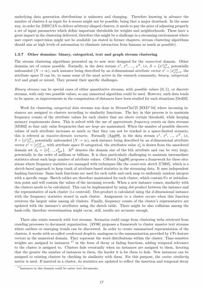
1.3.7 Other domains: binary, categorical, text and graph stream clustering

The stream clustering algorithms presented up to now were designed for the numerical domain. Otherdomains are of course possible. Formally, in the data stream x1, x2, ..., xN , i.e, S = xiNi=1 potentiallyunbounded (N →∞), each instance being described by an d-dimensional attribute vector xi = [xij ]dj=1, theattribute space Ω can be, to name some of the most active in the research community, binary, categorical,text and graph or mixed. They present their specific challenges.

Binary streams can be special cases of either quantitative streams, with possible values 0, 1, or discretestreams, with only two possible values, so any numerical algorithm could be used. However, such data tendsto be sparse, so improvements in the computation of distances have been studied for such situations [Ord03].

Work for clustering categorical data streams was done in StreamCluCD [HXD+04] where incoming in-stances are assigned to clusters according to similarity functions. The key in this process is to maintainfrequency counts of the attribute values for each cluster that are above certain threshold, while keepingmemory requirements down. This is solved with the use of approximate frequency counts on data streams[MM02] so that only value frequencies that are large are maintained. When the number of possible discretevalues of each attribute increases so much so that they can not be tracked in a space-limited scenario,this is referred as massive-domain scenario. Formally [Agg09], in the data stream x1, x2, ..., xN , i.e,S = xiNi=1 potentially unbounded (N →∞), each instance being described by an d-dimensional attributevector xi = [xij ]dj=1, with attribute space Ω categorical, the attributes value xik is drawn from the unordereddomain set Jk = vk1 , ..., vkMk. Mk denotes the domain size of the kth attribute and can be very large,potentially in the order of millions or billions. It is then particularly challenging to maintain intermediatestatistics about such large number of attribute values. CSketch [Agg09] proposes a framework for these situ-ations where frequency statistics are managed with techniques like the count-min sketch [CM05], which is asketch-based approach to keep track of attribute-based statistics in the streaming data. It uses independenthashing functions. Same hash functions are used for each table and each map to uniformly random integerswith a specific range. Sketch tables are therefore maintained for each cluster, which contain 0’s at initializa-tion point and will contain the values of the incoming records. When a new instance comes, similarity withthe clusters needs to be calculated. This can be implemented by using dot-product between the instance andthe representative of each cluster (i.e centroid). Dot-product is calculated using the d-dimensional instancewith the frequency statistics stored in each cluster. Assignment to a cluster occurs when this functionretrieves the largest value among all clusters. Finally, frequency counts of the cluster’s representative areupdated with the instance’s attributes using the sketch table. There might be also collisions among thehash-cells, therefore overestimation might occur, still, results are accurate enough.

There also exists research with text streams. Scenarios could range from clustering webs retrieved fromcrawling processes to document organization. [AY06] proposes a framework to cluster massive text streamswhere outliers or emerging trends can be discovered. In order to create summarized representation of theclusters, it works with so-called condensed droplets, analogous to the summarization provided by CFs featurevectors in the numerical domain. They represent the word distributions within the cluster. Time-sensitiveweights are assigned to instances 17 in the form of decay or fading functions, adding temporal relevanceto the cluster is assigned to. Clusters fade eventually when no instances are assigned to them, favoringthat the greater the number of instances in them, the harder it is for them to fade. New instances can beassigned to existing clusters by checking its similarity with them. For this purpose, the cosine similaritymetric is used. If inserted in a cluster, its statistics are updated to reflect the insertion and temporal decay

17Instances in this domain could be entire text documents.

17

statistics. A different approach to text stream clustering is presented in [HCL+07] with the use of so-calledbursty features, designed to highlight temporal important features in text streams, and therefore detect newemerging topics (different from clustering the underlying data stream). They are based on the concept thatsemantics of a new topic is marked by the appearance of a few distinctive words in the stream and thatthey dynamically represent documents better over time. These features are identified by using Kleinberg’s2-state finite automation model [Kle02]. Then, time-varying weights are assigned to the features by the levelof burstiness. Identification and weighting of the bursty features are dependent on occurrence frequency.Finally, standard k-means is used to provide final clustering based on the new representations of the stream.

Clustering massive graph streams tries to bring together sound graph theory with stream processing.Graphs are very interesting structures because they are very flexible and capture information very effectively,and seem natural candidates to capture, for instance, data coming from social or information networks,which are producing large amounts of data every single day. While there are methods for clustering graphs[RMJ07], [FTT03], they are designed for static data and are not applicable with graph streams. Also,massive graphs would present serious challenges for these techniques due to the large number of nodes andedges that need to be tracked simultaneously, which translates into storage and computational problems.Graph streaming is therefore a topic of intense research. Depending on the type of incoming instance inthe stream and the task to accomplish, we can distinguish two sort of situations: node clustering and objectclustering. In node clustering situations, each incoming instance is a node or an edge of a graph (that is,we are clustering one single graph and not a stream of different graphs) and the task is to carry out is todetermine general dynamic community detection. On the other hand, object clustering tackles situationswhere incoming instances are graphs drawn from a base domain, containing nodes and edges, and thesegraphs are clustered together based on their structural similarity.

Regarding node clustering, there is work related to outlier detection [AZY11], where detection focuseson structural abnormalities or different from ”typical behavior” of the underlying network. This shows inthe form of unusual connectivity structure among different nodes that are rarely linked together. Unusualconnectivity structures can only be defined using historical connectivity structures, therefore the need tomaintain structural statistics. The network is thus dynamically partitioned using structural reservoir sam-pling approach and maintains structural summaries of the underlying graph. Conceptually, node partitionsrepresent dense regions in the graph, so rare edges crossing those dense regions are exposed as outliers. Thealgorithm does not handle updates in the graph (i.e deletions), only additions to the graph. While this workfocuses on outlier graph detection and detects node clustering in an intermediate phase, [EKW12] providesspecific dense node clustering in graph streams by refining the structural reservoir sampling. The algorithmhandles time-evolving graphs where updates are given in the form of stream of vertex or edge additions anddeletions in an incremental manner, which can be easily parallelized.

Object clustering arises from the applications where information is transmitted as individual graphs. Thiscould be the case in movie databases where actors and films are nodes and edges are the relationships amongthem. In these applications, small graphs are created or received, having the assumption that the graphscontain only a small fraction of the underlying nodes and edges. This sparsity property is typical for massivedomains. It gives raise to the problem of handling, representing and storing the fast incoming graphs.GMicro algorithm [AY10] proposes hash-compressed micro-clusters from graph streams. It combines theidea of sketch-based compression with micro-cluster summarization. This is very useful in cases like massivedomain on the edges, where number of distinct edges is too large for the micro-cluster to maintain statisticsexplicitly. Graph micro-clusters contain, among others, a sketch-table of all the frequency-weighted graphswhich are added in the micro-cluster. Intermediate computations, like distance estimations, can then beperformed as sketch-based estimates while maintaining effectiveness. Additional work to discover significant(frequently co-occurring) and dense (node sets that are also densely connected) subgraphs in the incomingstream shows in [ALY+10]. A probabilistic min-hash approach is used to tackle sparsity, summarize thestream and efficiently capture co-occurrence behavior efficiently or patterns.

18

1.4 Technology platforms used

1.4.1 MOA (Massive Online Analysis)

As stated before, the requirements for this master thesis is the creation of a new stream clustering algorithm,its integration in MOA platform (Massive Online Analysis) and benchmark analysis against state of the artcompetitors.

Figure 6: MOA’s logo

We accessed the available documentation18 ([BHK+11], [BK12], [BK+12], [Str+13]) and check MOA’scapabilities so that we make sure that it has the proper features we need for the project:

- MOA is a specialized platform for data stream mining developed by the University of Waikato, NewZealand. 19. It is well-known and accepted in the research community and includes a collection of machinelearning algorithms, ranging from classification, regression, clustering, outlier detection, concept drift detec-tion and recommender systems. Project leaders are Albert Bifet, Geoff Holmes and Bernhard Pfahringerand contributors Ricard Gavalda, Richard Kirkby or Philipp Kranen among others.

- MOA has portable architecture. Related to the WEKA project, it can scale to more demanding problems.This is achieved by using JAVA as programming language.

- MOA is open source, follows modular design able to accommodate new algorithms and metrics. Thisis done via interfaces:

Figure 7 shows the internal modules and workflow used in MOA.

Figure 7: MOA’s workflow to extend framework

We will therefore plug-in our logic in two places in the framework:

- data feed/generator : here we will feed real data to be turned into a stream so that we can benchmark ouralgorithm against the others.- learning algorithm: we will integrate our new algorithm in this section.

18http://moa.cms.waikato.ac.nz/documentation/19(http://moa.cms.waikato.ac.nz/)

19

- MOA provides an application program interface API. It is then possible to use methods of MOA in-side JAVA code. We will use these in order to implement our algorithm and integrate within MOA.

To add a new stream clustering algorithm, we need to implement the Clusterer.java interface with thefollowing three main methods:

void resetLearningImpl(): a method for initializing a clusterer learner.void trainOnInstanceImpl(Instance): a method to train a new instance.Clustering getClusteringResult(): a method to obtain the current clustering result for evaluation or visual-ization.

- MOA generates synthetic streaming data20: synthetic stream data generation is achieved through RBF(Radial Basis Function) data generators 21, which are normalized in the [0,1] range.

- MOA streaming of real data provided by user22: real data can be fed to MOA and turned into a streamby providing a data file and adding headers that specify how to stream the different fields and/or potentialnormalization of the data.

- MOA has basic stream visualization capabilities23 by choosing specific dimensionality. Still, visualiz-ing multi-dimensional streaming data is challenging and a field of research on its own.

- MOA has the ability to run several competing algorithms in parallel24.

- MOA can gather, visualize and export clustering quality statistics, based on a set of metrics availablefor clustering evaluation25.

- MOA allows to perform tasks via command line interface:

this is important for our scalability and sensitivity tests. As an example, the command

EvaluateClustering -l clustream.Clustream -s (RandomRBFGeneratorEvents -K 2 -k 0 -R 0.025 -n -E 50000-a 5) -i 500000 -d dumpClustering.csv

evaluates the runtime performance of the Clustream algorithmm with a synthetic feed random RBF gener-ator, creating 500000 data instances for the stream, of 2 clusters, with no variation in number of clusters,cluster radius 0.025 in normalized space, no creation/deletion/merge/split cluster event, which would oth-erwise occur every 50000 instances26. The results would be dumped into the dumpClustering.csv file (forfurther analysis).

20See figures 8 for configuration, section 3.21See Appendix on Streaming Terminology for further details.22See figures 8 for configuration, section 3.23See figure 9 for visualization, section 8.24See figures 8 for configuration, section 3.25See figure 8 for export, figure 9 for visualization, section 9.26There are other values that are set by default, like no variation in cluster’s radius, noise level 10 percent, etc.

20

- Finally, we will launch the MOA27 application from the command line. First indicate where the soft-ware is located:

cd c : \MOA 2014 11set MOADIR = C : \MOA 2014 11

then set the CLASSPATH variable so that JAVA can find the .jar files:

set CLASSPATH = .; %MOADIR%\moa.jar; %MOADIR%\sizeofag.jar; %CLASSPATH%28

and finally launch the application to start up the main GUI:

java −javaagent : sizeofag.jar moa.gui.GUI

MOA’s task configuration GUI is shown in Figure 8.

Figure 8: MOA’s clustering task configuration GUI

27MOA Release 2014.11 (http://moa.cms.waikato.ac.nz/downloads/) was used since it was the latest official release at thetime of starting this thesis. At the time of writing this document, a new pre-release was available MOA Pre-Release 2015.05

28For the implementation of the new algorithm, we will use a JAVA mathematical library called commons-math3-3.5.jar. TheApache Commons Math project is a library of lightweight, self-contained mathematics and statistics components addressing themost common practical problems not immediately available in the Java programming language or commons-lang. Thereforethe additional .jar component will be added to the CLASSPATH(http://commons.apache.org/proper/commons-math/download_math.cgi)

21

And the corresponding clustering task visualizatio in Figure 9:

Figure 9: MOA’s clustering task visualization GUI

1.4.2 JAVA

We need to integrate our algorithm in MOA, which is implemented in JAVA. We will use Eclipse:

Eclipse IDE for Java DevelopmentVersion: Kepler ReleaseBuild id: 20130614-0229

We will compile the classes containing our new algorithm:

javac LeaderKernel.javajavac LeaderStream.java

then place the generated .class files (LeaderKernel.class and LeaderStream.class) under the directory createdfor the new logic 29,

%MOADIR%\moa\clusterers\StreamLeader

and finally launch the application to start up the main GUI with the new algorithm showing in the appli-cation30:

java −javaagent : sizeofag.jar moa.gui.GUI

1.4.3 R

In order to carry out statistical analysis and plots needed for the design, analysis and graphs used for testsvisualization of the results from MOA, R was chosen.

R is a free software environment for statistical computing and graphics. It compiles and runs on a widevariety of UNIX platforms, Windows and MacOS. The software version:

29Respecting MOA’s folder structure for the location of stream clustering algorithms.30See Figure 8: MOA’s clustering task configuration GUI, area 3 in circle, where the new algorithm should be now available.

22

R version 3.0.1 (2013-05-16).

We used R Studio as IDE for R:

R Studio, an open source IDE for R development

Version 0.97.551

1.5 Main competitors in MOA

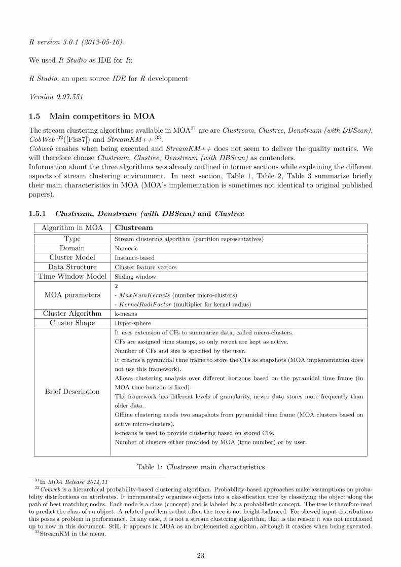
The stream clustering algorithms available in MOA31 are are Clustream, Clustree, Denstream (with DBScan),CobWeb 32([Fis87]) and StreamKM++ 33.Cobweb crashes when being executed and StreamKM++ does not seem to deliver the quality metrics. Wewill therefore choose Clustream, Clustree, Denstream (with DBScan) as contenders.Information about the three algorithms was already outlined in former sections while explaining the differentaspects of stream clustering environment. In next section, Table 1, Table 2, Table 3 summarize brieflytheir main characteristics in MOA (MOA’s implementation is sometimes not identical to original publishedpapers).

1.5.1 Clustream, Denstream (with DBScan) and Clustree

Algorithm in MOA ClustreamType Stream clustering algorithm (partition representatives)

Domain NumericCluster Model Instance-basedData Structure Cluster feature vectors

Time Window Model Sliding window

MOA parameters2- MaxNumKernels (number micro-clusters)- KernelRadiFactor (multiplier for kernel radius)

Cluster Algorithm k-meansCluster Shape Hyper-sphere

Brief Description

It uses extension of CFs to summarize data, called micro-clusters.CFs are assigned time stamps, so only recent are kept as active.Number of CFs and size is specified by the user.It creates a pyramidal time frame to store the CFs as snapshots (MOA implementation doesnot use this framework).Allows clustering analysis over different horizons based on the pyramidal time frame (inMOA time horizon is fixed).The framework has different levels of granularity, newer data stores more frequently thanolder data.Offline clustering needs two snapshots from pyramidal time frame (MOA clusters based onactive micro-clusters).k-means is used to provide clustering based on stored CFs.Number of clusters either provided by MOA (true number) or by user.

Table 1: Clustream main characteristics31In MOA Release 2014.1132Cobweb is a hierarchical probability-based clustering algorithm. Probability-based approaches make assumptions on proba-

bility distributions on attributes. It incrementally organizes objects into a classification tree by classifying the object along thepath of best matching nodes. Each node is a class (concept) and is labeled by a probabilistic concept. The tree is therefore usedto predict the class of an object. A related problem is that often the tree is not height-balanced. For skewed input distributionsthis poses a problem in performance. In any case, it is not a stream clustering algorithm, that is the reason it was not mentionedup to now in this document. Still, it appears in MOA as an implemented algorithm, although it crashes when being executed.

33StreamKM in the menu.

23

Algorithm in MOA DenstreamType Stream clustering algorithm (density-based)

Domain NumericCluster Model Instance-basedData Structure Cluster feature vectors

Time Window Model Damped or fading window

MOA parameters

7- ε (neighborhood around micro-clusters)- β (outlier threshold)- µ (weight of micro-clusters)- initPoints (initialization)- offline (multiplier for ε)- λ (defines decay factor)- processingSpeed (incoming points per time unit)

Cluster Algorithm DBSCANCluster Shape Arbitrary-shaped

Brief Description

It uses CFs or micro-cluster to summarize the data.No limit on number of micro-clusters but constrain on radius & weight.p-micro-clusters keep track of potential clusters.o-micro-clusters keep track of potential outliers.Weight time aging fading for p-micro-clusters, using decay function.p-micro-clusters below a threshold turns into o-micro-clusters.Offline clustering based on DBSCAN.It builds the concept of density reachable & density connected regions.Number of clusters non predefined.

Table 2: Denstream main characteristics

Algorithm in MOA ClustreeType Stream clustering algorithm (partition representatives)

Domain NumericCluster Model Instance-basedData Structure Cluster feature vectors

Time Window Model Damped or fading window

MOA parameters 1- MaxHeight (maximum height of the tree)

Cluster Algorithm k-meansCluster Shape hyper-sphere

Brief Description

It uses CFs to summarize the data.It uses fast indexing structure, R Tree, to store and maintain CFs.Temporal information is assigned to nodes and CFs which decay with time.R Tree allows computation of distances in logarithmic time, therefore insertions are loga-rithmic in the number of CFs maintained.Entries in node are split into 2 groups so that sum of intra-group distances is minimal.The further down in the tree, the more fine-grained the resolution of the micro-clusters.There are different descend strategies inside the tree.It implements any-time clustering, interrupting the process any time can deliver clustering.With enough time, instances descend through the tree to the most similar CF. When nosuch CF is found, a new is created.Buffers in nodes for instances whose descend was interrupted. They are called Hitchhikers.New instances descending can take Hitchhikers with them.Offline algorithm can be anything, k-means or DBSCAN (k-means in MOA).

Table 3: Clustree main characteristics

24

2 Part 2 - StreamLeaderNow that we reviewed the state of the art and chose the platforms for development, we focus on the designof the new stream clustering algorithm.

2.1 Conventional Leader clustering algorithm

As stated in the goals section, basic requirement for the new algorithm is that it must follow the principlesof the Leader clustering algorithm in batch mode, as specified by John Hartigan in Clustering Algorithms in[Har75]. In Table 4 we can find the algorithm as it was originally presented and also adapted to structuredprogramming:

INPUT: T maximum distance around each leader clusterOUTPUT: L List of clusters

I: actual instanceM : total number of instancesJ : actual clusterK: number of clustersP (x): function that indicates to which cluster belongs instance xL(x): function that indicates the Leader of cluster number xT : maximum distance d max (as a distance metric)(function d would be defined as Euclidean distance metric)

Leader algorithm(as presented by Hartigan)

Leader algorithm(adapted to structured programming)

start1 I := 12 K := 13 P (I) := K4 L(K) := I5 I + +6 if I > M , stop7 else if I ≤ M then8 J := 19 if d(I, L(J)) > T10 goto 1511 elseif d(I, L(J)) ≤ T then12 P (I) := J13 goto 514 endif15 J + +16 if J ≤ K17 goto 918 elseif J > K then19 K + +20 P (I) := K21 L(K) := I22 goto 523 endif24 endifend

start1 I := 12 K := 13 P (I) := K4 L(K) := I5 while I ≤M do6 J := 17 while J ≤ K and P (I) = 0 do8 if d(I, L(J)) ≤ T then9 P (I) := J10 end if11 J + +12 end while13 if P (I) = 0 then14 K + +15 P (I) := K16 L(K) := I17 end if18 I + +19 end whileend

Table 4: Conventional Leader clustering algorithm

25

As we can see, the Leader is a partition clustering algorithm, very straightforward and fast. We outlineits behavior:

As input, it receives (in its original version) a distance threshold T . This is the influence of each leader inits neighborhood. In this case, the influence was defined as Euclidean distance.

As output, it returns a list with the resulting clusters.

At the very beginning, first instance creates a cluster on its own and represents it as the leader of thatcluster.When a cluster is created for the first time, the instance that created it remains as the leader of that cluster,forever. That is, it will be its representative and will not change, even if more instances are assigned to thatcluster.

When a new instance is taken for analysis, it is checked against the clusters.That means, it is checked against the leaders that represent each cluster, one by one until we find the firstcluster (leader) which area of influence includes the instance. We notice that ordering is quite importantin two ways. The order in which checking is done against the leaders could influence the assignation toone cluster or another that also fulfills the proximity criteria. On the other hand, the ordering of the in-stances decides which ones create clusters and leaders (first instances usually create the clusters) and whichinstances are assigned to those already existing clusters. Different ordering in batch processing producesdifferent clustering.

We also notice that checking area of influence is dependent of the similarity metric that can be used.In this case, the original algorithm was designed to work with distances (parameter T ). But we see that thedefinition of this similarity metric is quite important since it defines how clusters are formed.

When an instance is assigned to a cluster, the leader of that cluster is not altered because of the newaddition.If the instance is checked against all leaders and none of them is close enough (similar enough), then a newcluster is created with the new instance as the leader.

We can already draw some basic conclusions:

- Our new stream clustering algorithm needs to be inspired in the leader concept, specifically in how clustersare created from instances that were not assigned to any cluster and how leaders represent them.

- We already notice that the definition of a leader is quite static; they are assigned once and remainfixed (keep if physically) for the entire existence of a cluster. This will be for sure a problem in a dynamicstreaming environment with concept drift and instance processed only once policy.

- A decisive factor is the ordering. As stated already, in a streaming environment we will have no con-trol on the ordering of the incoming instances.

- We should keep its simplicity and make it as fast as possible.

- We already know we should receive a parameter specifying the influence of the leader on the surroundingarea, which in this case is Euclidean distance. We will need to consider what proximity measure we will use.

- Last but not least, we should try as hard as possible to create high quality clustering in a streamingenvironment because we will compete against state of the art Clustream, Denstream and Clustree.

- We will name our new algorithm StreamLeader

26

2.2 Strenghts and weaknesses of Clustream, Denstream and Clustree

Before taking on the design of the new StreamLeader, we want to come up with a list of key characteristics wewant the new algorithm to have. That is, make it as robust, fast and accurate as possible while eliminatingpotential weaknesses. In order to do that, a good strategy is to carefully analyze the competing algorithmsand see what advantages and disadvantages they posses. This will be a good starting point to start designing,by detecting their strengths and weaknesses (if any).

We analyze with spacial care the original research papers for Clustream, Denstream and Clustree andalso their JAVA implementation in MOA. Furthermore, we take into considerations the techniques andalgorithms reviewed in the state of the art section.

We draw some interesting conclusions based on their design:

Key strengths:

- Online phase: they achieve data abstraction quite successfully through use of extensions of ClusterFeature Vectors. Other algorithms use grid cells, which would be more oriented to density-based solutionswhich is not what we aim for. Furthermore, tree coresets, while effective, are complicated structures toconstruct and maintain, which might take a toll on performance and simplicity.

- Shape: Denstream can produce arbitrary-shaped clustering using the offline clustering step. Clustreamand Clustree build hyper-spheric Gaussian constructs (which is more restrictive).

Key weaknesses:

- Offline phase. They all share it and is always present when clustering determination is required at aspecified moment. They all require standard batch clustering technique (like k-means, DBSCAN, etc) toproduce final clustering based on the data abstraction provided by online step. This applies to Clustream,Denstream, Clustree. We tend to think that it slows down the whole process.

- Complexity in parametrization: Denstream would require an expert to fine-tune the set of severalparameters in a changing streaming environment, which seems a considerable challenge. On the other hand,Clustream requires a number of micro-clusters proportional to the number of natural clusters (also calledmicro-ratio) of, at leasts, 10 to 1. Such ratio should be unknown and also changing.

- Speed issues: maintainance of high number of micro-clusters. Clustream, Denstream and Clustree arebased on the assumption that the more micro-clusters they can (efficiently) manage, the finer the dataabstraction granularity would be passed to the offline components for final clustering, and therefore thebetter the quality of the clustering produced. We tend to think that more micro-clusters might providemore granularity, but also more memory consumption. Also, if we could envisage an alternative in order tonot use conventional algorithm for final clustering, maintaining great numbers of micro-clusters would notbe needed at all.

- Noise issues: If CF micro-clusters map also noise in the online step, it is also natural to think that theoffline clustering algorithm based on the micro-clusters might have difficulties discarding noise from databelonging to true clustering. Determined clustering might be then affected by noise. Noise managementmight be an issue for some of the algorithms, transparent for the user and ideally not dependent on anyuser parametrization.

- Multidimensionality and accuracy: The fact that micro-clusters abstract sets of data instances in thed-dimensional space and are later used as points for clustering determination (using conventional clustering),lead us to think that high dimensional spaces would yield bigger and bigger multi-dimensional micro-clusters.If that is the case, they would potentially fill more and more the space. On top, offline clustering based onover-inflated micro-clusters might tend to produce over-sized clustering, with clusters overlapping amongthem. It is natural to think that, if occurring, we would also expect low levels of recall and accuracy inclustering metrics.

27

2.3 Design strategy

With these factors in mind, we design the StreamLeader with the aim of keeping or enhancing the strengthsand eliminating or at least diminishing the weaknesses they all seem to share.

We aim to integrate the following key pieces in the StreamLeader’s design:

- Online component: clustering feature vectors CFs. We use the CF concept to create abstractions ofthe data, what are called in the literature micro-clusters. We will extend them with additional capabilitiesto confer them as much flexibility as possible. We will name our special micro-clusters LeaderKernels, eachone representing a potential natural cluster.

- Online component: each dimension in d space with range [0,1]. Our algorithm and the LeaderKernelswill work by scaling the d-dimensional space observations of the stream into a space where each dimen-sion (attribute) is restricted to [0,1]. This concept fits well with MOA synthetic data generation, whichgenerates random RBF generators34, Gaussian hyper-spheres, constraining each artificial attribute to [0,1]values in each dimension. Furthermore, real stream data can always be converted or approximated intothat space (as MOA does). An important factor is that we plan to give our generated clusters flexibility toexpand/contract if necessary to better adjust to the detected data. Working in the space described abovemaximizes our chances of achieving best results. Lastly, even if visualization will always be very restrictedwith conventional techniques, scaling down the data allows visualization and comparison of the data andclusters in MOA by selecting any two dimensions.

- Online component: spherical Gaussian-shaped clusters. The StreamLeader will create hyper-sphericalGaussian-shaped clusters. They will try to capture the center of masses of the detected clusters, startingoff initially with a maximum radius provided by the user (D MAX parameter).

- Online component: dynamic cluster size adaptation: We will give the LeaderKernels, the capabilityto dynamically override (contract/expand) its radius to a certain extend, with the aim to capture the datastructures with as much accuracy as possible. This will be different from standard merging in some situa-tions which is possible in other algorithms.

- Offline component: no offline conventional clustering algorithm to deliver final clustering. We will notuse offline standard batch clustering algorithm in batch mode (i.e k-means, DBSCAN, etc) as it is used byall other competitors. We want in this way to create a solution conceptually different to the other streamingalgorithms. Also, we aim for speed.

- Offline component: cluster size adjustment. When time window expires, StreamLeader will check po-tential merging of close-enough LeaderKernels to produce better final clustering.

- Offline component: noise elimination. When time window or horizon expires, StreamLeader will targetspecific statistical noise elimination automatically. We aim at two things: to be very resilient to noise andat the same time provide an alternative to offline conventional clustering based on CFs.

- Parametrization: only one user-friendly parameter will be required, D MAX. This parameter willindicate the area of influence that a leader from a LeaderKernel has in its neighborhood. Since we workin normalized d-dimensional space, it will be a distance measure35, with a range (0...0.5]. It determinesthe level of clustering to be produced. Smaller D MAX would discover small data structures and biggerD MAX would discover bigger ones within the data stream. Still, it will not be rigid as in the conventionalLeader algorithm, StreamLeader takes this parameter into consideration and tries to adapt the size of theLeaderKernels to the stream, adjusting to changing environments and detecting bigger or smaller structuresif it makes sense. This capability should render the algorithm much needed flexibility, having in mindthat we will not use conventional clustering as last step. This one-parameter approach therefore aims atsimplicity and understandability by any non expert user and the algorithm will use it in a flexible way.

34See Appendix with stream clustering definitions.35Further details about this important point will be discussed in next sections.

28

2.4 Cluster Feature Vectors: LeaderKernels

2.4.1 Framework and encapsulation

The data stream needs to be captured in some way without storing the single instances. We adhere tothe concept of one-pass algorithms where instances are only treated once and then discarded. In order todo that, we need to capture statistical information that describes the data stream. We achieve that byconstructing the LeaderKernels, as extensions of the cluster feature vectors CFs.

Definition 8 (LeaderKernel). We call a LeaderKernel in a d-dimensional normalized space, for a set ofinstances x1, x2, ..., xn, each described by an d-dimensional attribute vector xi = [xij ]dj=1 which belongs to anattribute space Ω that is continuous, with timestamps of arriving instances T 1,T 2, ..., Tn, with distances36

to leader37 (or LeaderKernel’s representative) of arriving instances D1,D2, ..., Dn as the tuple

(LS, SS, LST , SST , LSD, D MAX, N ,creation timestamp, is artificially expanded, artificially expanded radius)

where

- LS : vector of d entries.For each dimension, linear sum of all the instances added to the LeaderKernel. The p-th entry of LS is equalto

∑nj=1 x

jp.

- SS : vector of d entries.For each dimension, squared sum of all the instances added to the LeaderKernel. The p-th entry of SS isequal to

∑nj=1(xjp)2.

- LST : linear sum of the timestamps of all instances added to the LeaderKernel, equal to∑nj=1 T

j .

- SST : squared sum of the timestamps of all instances added to the LeaderKernel, equal to∑nj=1(T j)2.

- LSD: linear sum of the distances to the leader of all instances added to the LeaderKernel, equal to∑nj=1D

j .

- D MAX : influence of the LeaderKernel, taken its leader as representative, in its neighborhood in thenormalized d-dimensional space, measured in terms of the distance function, with range (0...0.5].

- N : Number of instances added to the LeaderKernel. Also designated as weight in this document.

- creation timestamp: timestamp that indicates when the LeaderKernel was created.

- is artificially expanded: boolean that indicates whether the LeaderKernel was artificially expanded far-ther than indicated by D MAX.

- artificially expanded radius: radius of the LeaderKernel as a result of an artificial expansion process.

We can refer to the LeaderKernel for a set of instances S by LK(S).

36Discussion on suitable proximity measures and distance function used will be explained in next sections.37Discussion on leader calculation will be explained in next sections. As we will see later, in original Hartigan’s algorithm,

the leader of a cluster was one of the physical points being analyzed in the point set and was static. On the other hand,StreamLeader will store no physical instance as such. Instead it will use the summarization stored in the LeaderKernel tocalculate the leader dynamically.

29

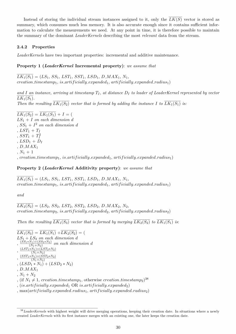
Instead of storing the individual stream instances assigned to it, only the LK(S) vector is stored assummary, which consumes much less memory. It is also accurate enough since it contains sufficient infor-mation to calculate the measurements we need. At any point in time, it is therefore possible to maintainthe summary of the dominant LeaderKernels describing the most relevant data from the stream.

2.4.2 Properties

LeaderKernels have two important properties: incremental and additive maintenance.

Property 1 (LeaderKernel Incremental property): we assume that

LK1(S1) = (LS1, SS1, LST1, SST1, LSD1, D MAX1, N1,creation timestamp1, is artificially expanded1, artificially expanded radius1)

and I an instance, arriving at timestamp TI , at distance DI to leader of LeaderKernel represented by vectorLK1(S1).Then the resulting LK1(S2) vector that is formed by adding the instance I to LK1(S1) is:

LK1(S2) = LK1(S1) + I = (LS1 + I on each dimension d, SS1 + I2 on each dimension d, LST1 + TI, SST1 + T 2

I

, LSD1 + DI

, D MAX1, N1 + 1, creation timestamp1, is artificially expanded1, artificially expanded radius1)

Property 2 (LeaderKernel Additivity property): we assume that

LK1(S1) = (LS1, SS1, LST1, SST1, LSD1, D MAX1, N1,creation timestamp1, is artificially expanded1, artificially expanded radius1)

and

LK2(S2) = (LS2, SS2, LST2, SST2, LSD2, D MAX2, N2,creation timestamp2, is artificially expanded2, artificially expanded radius2)

Then the resulting LK1(S3) vector that is formed by merging LK2(S2) to LK1(S1) is:

LK1(S3) = LK1(S1) +LK2(S2) = (LS1 + LS2 on each dimension d, (SS1∗N1)+(SS2∗N2)

(N1+N2) on each dimension d

, (LST1∗N1)+(LST2∗N2)(N1+N2)

, (SST1∗N1)+(SST2∗N2)(N1+N2)

, (LSD1 ∗N1) + (LSD2 ∗N2), D MAX1, N1 +N2, (if N1 6= 1, creation timestamp1, otherwise creation timestamp2)38

, (is artificially expanded1 OR is artificially expanded2), max(artificially expanded radius1, artificially expanded radius2)

38LeaderKernels with highest weight will drive merging operations, keeping their creation date. In situations where a newlycreated LeaderKernels with its first instance merges with an existing one, the later keeps the creation date.

30

LeaderKernels summarize information about instances contained in them by using incremental properties(adding new instances to an existing LeaderKernel) or additive (merging two LeaderKernels). At anymoment, statistical information about the instances contained in the relevant LeaderKernels are maintained.When a LeaderKernel summarizes instances that are not relevant anymore, then they are eliminated bymeans of elimination of the corresponding LeaderKernel. This is the case of either noise or out-of-dateinformation. These two points will be discussed in detail in next sections.

2.4.3 Proximity measure: distance function in normalized space

Since clustering require grouping homogeneous but distinct objects among them, a key aspect for most ofthe clustering algorithms in general is the proximity measure between pairs of objects in the space we areworking. It reflects the actual proximity between instances according to the final aim of the clustering.Weighting the attributes might be sometimes necessary.

Before deciding which proximity measure StreamLeader and LeaderKernel will use, we can review whatoptions we have. Then we will take an informed decision on this important step.

Proximity measures range from distance to distance indexes, similarity and dissimilarity indexes, depend-ing on the properties they hold. Distances are very popular in literature. When it comes to dealing withnumerical data, Minkowsky distances in Lp norm can be used, where relation between norm and distance is

D(I1, I2) = ||I1 − I2||

and L p norm is the distance induced by norm Lp

Lpnorm→ Dp(I1, I2) = ||I1 − I2||p = (d∑i=1|I1i − I2

i |p)1/p

in a d-dimensional spaceand particular cases, for instance,

L1 → DManhattan(I1, I2) = ||I1 − I2||1 =d∑i=1|I1i − I2

i |

L2 → DEuclidean(I1, I2) = ||I1 − I2||2 =

√√√√ d∑i=1

(I1i − I2

i )2

L∞ → DChebyshev(I1, I2) = ||I1 − I2||∞ = maxi|I1i − I2

i |

We can see in Figure 10 the kind of unit circles generated in the space for various values of p39. Theyshow the contour of the equidistances:

Figure 10: Minkowski distances for various values of p

Proximity measures are taken according to clustering needs. While all distances shown above are equidis-tant to the centers of the unit circles, L2 DEuclidean results from scalar product and is a natural choice torepresent distances in d-dimensional space40. Many stream algorithms choose L2, StreamKM++ [AMR+12],Clustream [AHWY03], Clustree [KABS11] Denstream [CEQZ06] and BIRCH [ZRL97], among others.

39Picture taken from Wikipedia: https://en.wikipedia.org/wiki/Minkowski_distance.40It can also be more sensitive to outliers than other distance definitions.

31

Another important aspect to consider is MOA. It generates synthetic data by creating numerical (i.e.not textual, not heterogeneous) streams. This already constrains the sort of measure we can create sinceit must be based on numeric attributes. Also, the on-the-fly calculation of the ground-truth seems to bebased on distances by creating the smallest hyper-sphere that can capture the instances belonging to thesame class.

Still, we can already glimpse into the future with further possibilities in terms of creating distances forlogical, categorical data or strings data for example.

So we are ready to design our distance measure. As we stated before, StreamLeader will work, for the timebeing, in a normalized d-dimensional space, where each dimension is within [0,1], with instances describedby an d-dimensional attribute vector xi = [xij ]dj=1 which belongs to an attribute space Ω continuous.

L2 DEuclidean, if d large enough, can render distance values greater than 1. In order to fit into a normal-ized space, we will constrain those values to a maximum of 1. The pseudo-code for the distance functionlooks as follows:

FUNCTION: DISTSLINPUT: I1, I2 stream data instances in d-dimensional space (or any object in that same d-dimensionalspace, like a leader representing a LeaderKernel)OUTPUT: D distance between the two given instances I1, I2

1 d← dimensionality of I12 D ←

√∑di=1(I1

i − I2i )2

3 D ← DD+1

4 return D

Theorem 1 (DISTSL metric distance): if L2 DEuclidean√√√√ d∑i=1

(I1i − I2

i )2

is a metric distance with the following properties for S a massive sequence of instances, x1, x2, ..., xN , i.e,S = xiNi=1, each instance described by an d-dimensional attribute vector xi = [xij ]dj=1 which belongs to anattribute space Ω that is continuous

DISTSL : S × S → IR+

1. ∀xi ∈ S DISTSL(xi, xi) = 02. ∀xi, ∀xj ∈ S DISTSL(xi, xj) = 0→ xi = xj

3. ∀xi, ∀xj ∈ S DISTSL(xi, xj) = DISTSL(xj , xi)4. ∀xi,∀xj , ∀xk ∈ S DISTSL(xi, xk) ≤ DISTSL(xi, xj) +DISTSL(xj , xk)

then DD+1 and therefore DISTSL are also a metric distance with the same properties.

32

2.4.4 Hyper-spherical clustering: LeaderKernels’s leader

With the distance function above, the clusters created will be of hyper-spherical shape. Checking proximityof an incoming instances to the LeaderKernel will be done by applying the distance function between theinstance and the leader (representing the LeaderKernel). In non-streaming environments, a cluster’s repre-sentative could be calculated in different ways. Sometimes data points from the original set of points canbe taken as representatives, like k-medoids in [KR87]. Such approaches are not possible in pure conceptualstreaming, which adheres to the concept that data is discarded after being processed first time. Thereforeincoming instances should not be stored, even if they act as representatives of a whole cluster.41 Leadercalculation is simple using the statistical summaries:

FUNCTION: GET LEADERINPUT: ∅OUTPUT: L as statistical center of the LeaderKernel in d-dimensional space

1 L← LSN on each dimension2 return L

2.4.5 D MAX: area of influence of a leader

StreamLeader will only require one user-defined parameter, which is the influence of the leader in its d-dimensional space neighborhood, with range (0..0.5] on each of the d dimensions. The influence or proximitywill be measured in terms of the distance function we defined above. It determines the level of clustering tobe produced. Smaller D MAX would discover smaller data structures and bigger D MAX would discoverbigger ones within the data stream. As mentioned before, StreamLeader will have the flexibility to discoverand adjust to clusters of larger and smaller size than the area specified by radius D MAX. We will discussthese capabilities in next sections.

2.4.6 Creation (instance-based)

With the definitions above, we can already specify how a LeaderKernel can be created from one instance:

PROCEDURE: CREATEINSTANCE BASED

INPUT: I stream data instance, d dimensions, TS timestamp for addition of I to LeaderKernel, DMAXradio of influence of this LeaderKernel, TSTMP creation timestamp for creation of LeaderKernelOUTPUT: ∅

1 N ← 12 LS ← I on each dimension3 SS ← I2 on each dimension4 D MAX ← DMAX5 LST ← TS6 SST ← TS2

7 creation timestamp← TSTMP creation8 LSD ← 09 is artificially expanded← false10 artificially expanded radius← 0

41Relaxation on this rule can however be applied although is not the preferred approach in state or the art algorithms.

33

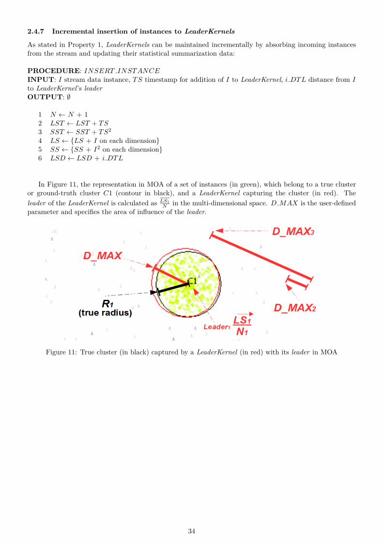
2.4.7 Incremental insertion of instances to LeaderKernels

As stated in Property 1, LeaderKernels can be maintained incrementally by absorbing incoming instancesfrom the stream and updating their statistical summarization data:

PROCEDURE: INSERT INSTANCEINPUT: I stream data instance, TS timestamp for addition of I to LeaderKernel, i DTL distance from Ito LeaderKernel’s leaderOUTPUT: ∅

1 N ← N + 12 LST ← LST + TS3 SST ← SST + TS2

4 LS ← LS + I on each dimension5 SS ← SS + I2 on each dimension6 LSD ← LSD + i DTL

In Figure 11, the representation in MOA of a set of instances (in green), which belong to a true clusteror ground-truth cluster C1 (contour in black), and a LeaderKernel capturing the cluster (in red). Theleader of the LeaderKernel is calculated as LS1

N in the multi-dimensional space. D MAX is the user-definedparameter and specifies the area of influence of the leader.

Figure 11: True cluster (in black) captured by a LeaderKernel (in red) with its leader in MOA

34

2.4.8 Additive merging of two LeaderKernels

As stated in Property 2, additive property implies that two different LeaderKernels can merge by absorbingone the other. Their statistical summarizations are then combined following the pseudo-code below:

PROCEDURE: MERGEINPUT: lkadd LeaderKernel to be absorbedOUTPUT: ∅

1 radius← get radius2 radius lk ← get radius from lkadd3 creation timestamp lk ← get creation timestamp in lkadd4 N lk ← num instances contained in lkadd5 LS lk ← LS in lkadd6 SS lk ← SS in lkadd7 LST lk ← LST contained in lkadd8 SST lk ← SST contained in lkadd9 LSD lk ← LSD contained in lkadd10 is artificially expanded l← check if lkadd was artificially expanded11 creation timestamp← if N 6= 1, creation timestamp, otherwise creation timestamp lk 12 N ← N + N lk13 LST ← (N∗LST )+(N lk∗LST lk)

(N+N lk)

14 SST ← (N∗SST )+(N lk∗SST lk)(N+N lk)

15 LSD ← (N ∗ LSD) + (N lk ∗ LSD lk)16 is artificially expanded← is artificially expanded or is artificially expanded lk17 artificially expanded radius← max between radius and radius lk18 LS ← LS + LS lk19 SS ← (N∗SS)+(N lk∗SS lk)

(N+N lk)

In Figure 12, on the left, we observe true clusters C0 and C1 formed by corresponding instances in adata stream. LeaderKernels LK0, LK1 (in red contour) capture them. On the right, due to concept drift,C0, C1 move close enough to merge. LK ′0 is the resulting LeaderKernel containing the combined statisticsof C0, C1 and capturing the combined mass. We observe how the center of gravity of LK ′0 needs to bere-calculated after the merging.

Figure 12: Two separate LeaderKernels (left) which get close enough and merge (right)

35

2.4.9 Set artificial expansion

As we will see in next sections, LeaderKernels can be artificially expanded. This will happen when Stream-Leader decides that D MAX is not large enough to capture a specific true cluster that a LeaderKernel isalready detecting but can not capture entirely42. In these special cases, a larger radius than D MAX willbe given to try capturing as much instance mass43 as possible44.

PROCEDURE: SET ARTIFICIALLY EXPANDEDINPUT: IAE boolean indicating whether the LeaderKernel is artificially expandedOUTPUT: ∅

1 is artificially expanded← IAE

FUNCTION: IS ARTIFICIALLY EXPANDEDINPUT: ∅OUTPUT: IAE boolean indicating whether the LeaderKernel is artificially expanded

1 IAE ← is artificially expanded2 return IAE

PROCEDURE: SET ARTIFICIALLY EXPANDED RADIUSINPUT: AE Radius artificially expanded radius to be assigned to this LeaderKernel (overrides D MAXas radius)OUTPUT: ∅

1 artificially expanded radius← AE Radius

2.4.10 Radius: contraction capabilities

The aim of the LeaderKernel is to detect mass (well-defined groups of instances) in the d-dimensional space,and it will try to place the leader in the center using the GET LEADER function we already defined. Theremight be situations when LeaderKernel detects a true cluster and places itself properly in space but thearea of influence specified by D MAX could be too large to cover that natural cluster. In those cases, thedelivered cluster would cover the true cluster and, either empty space (if we are lucky) or just noise or worseelements from other clusters (which would take a hit in quality metrics like Precision45 and Recall46)

We therefore need to handle situations occurring when true clusters are smaller than what LeaderKernelcovers with D MAX. That is, we allow the LeaderKernel to contract in radius to adjust as much as possibleto the size of the natural cluster.

First we calculate the average distance of all instances added to the LeaderKernel to its center (we recallLSD contains the linear sum of the distances to the center of all instances added to the LeaderKernel):

FUNCTION: GET µ DISTANCE TO LEADERINPUT: ∅OUTPUT: D average distance to the leader representing the LeaderKernel (of all distances of all instancesto leader at the time they were added to the LeaderKernel)

1 D ← LSDN

2 return D

Second, if the LeaderKernel was artificially expanded47, then we return the artificial radius assigned to42Further details on this when we explain the flow of the StreamLeader algorithm.43The terms weight and mass are equal in this context and refer to the number of instances allocated to each LeaderKernel.44LeaderKernels might be allocated with a larger radio than D MAX in specific situations.45For detail definition of the metric, refer to quality metric section.46For detail definition of the metric, refer to quality metric section.47Further details on artificial expansion will be explained in next sections.

36

it. If not, we try to adjust the radius accordingly to the summarized average distance of the mass con-centrated in the LeaderKernel. We therefore need to be able to do that adjustment. Different densitiesin natural clusters can occur. If we thought of a situation where the cluster contains the instances moreor less in a homogeneous way, then, the instances located close to the center of the hyper-spheres wouldhave distances close to zero. On the other hand, instances located very close to the maximum boundary(radius R) would have distances close to R. We can then suppose that, if the cluster adjusts well to thegroup of instances, the average distance of all instances contained would be close to R

2 , which is what LSDN

or GET µ DISTANCE TO LEADER tries to represent. If we were to adjust D MAX perfectly for thatcluster, then D MAX

2 would match R2 and also LSD

N .

In Figure 13, C0 and C1 appear as true clusters formed by the corresponding instances and radiusR. If two LeaderKernels were to capture the true clusters with accuracy, then their leader would belocated very close to the center of the true clusters. If an instance is located in those centers, thenDISTSL(instance, leader) ≈ 0. An instance located in the contour of the hyper-sphere would haveDISTSL(instance, leader) ≈ RTRUE RADIUS . Lastly, an instance located at around 1/2 of the length ofthe true radius, would have DISTSL(instance, leader) ≈ RT RUERADIUS

2 . If the instances are homogeneouslydistributed in the cluster, we can then calculate the average distance µ of all instances to a center of aLeaderKernel as LSD0

N0in C0 and LSD1

N1in C1. This guides us in approximating the size of the true cluster.

As we will see in next section, we will use this information to assign a radius to the LeaderKernels.

Figure 13: Average µ distance of instances contained in a LeaderKernel (in red) to its leader is LSDN

If we had a LeaderKernel with D MAX influence that captures a cluster and it is off up to 20% on thesize of the detected mass (ideally detected mass would match true cluster), then we consider that D MAXis a good radio for the LeaderKernel and a good estimation of the radio of the true cluster. That is, we arecomfortable in regions of D MAX between 80% and 120% of the volume of instance mass we detect. Thefact that we take 20% as threshold and no other comes as an informed decision since we work in a normalizedspace, work with fast incoming and changing streaming data, work with statistical summarizations of thestream and we might have different grades of sparsity of data within the same cluster, among others. So20% flexibility seems a reasonable value.48

In Figure 14 we see that LeaderKernel LK1 (contour in red) does not contract its predefined D MAX

48Of course this threshold could change, but we prefer to carry out extensive sensibility analysis on the parametrization ofthe algorithm instead of the amount of flexibility we allocate to the StreamLeader.

37

radius and captures the true cluster C1 (contour in black). No contraction occurs because LSD1N1

fallswithin 20% of maximum deviation of D MAX

2 , which indicates that LeaderKernel LK1 captures with enoughaccuracy the true cluster C1.

Figure 14: LeaderKernel (in red) not contracting in C1 (reason LSD1N1

within D MAX2 ± 20%)

On the other hand, Figure 15 shows a situation where LeaderKernel LK0 (contour in red) contracts itspredefined D MAX radius in order to capture true cluster C0 (contour in black) better. Contraction takesplace because LSD0

N0falls outside the maximum deviation of 20% allowed for D MAX

2 . This indicates thatD MAX is a too large radius to capture C0 and LeaderKernel LK0 needs to contract to a smaller radius.

Figure 15: LeaderKernel (in red) contracts in C0 to the detected mass (reason LSD0N0

< 80% D MAX2 )

38

The logic behind the calculation of the adjustment is therefore based on the summarization of the dis-tances maintained applied to the hyper-spherical spheres of the LeaderKernels. If D MAX is off up to20% of detected mass, then we take D MAX as acceptable radio49. If it deviates more than 20% and thedetected mass seems of smaller size, then we return the radio we detect using only mass (LSDN ∗ 2) andignoring the guideline given by D MAX. The pseudo-code below shows how the radius is calculated. Wetherefore allow LeaderKernels to contract in radius as follows:

FUNCTION: GET RADIUSINPUT: ∅OUTPUT: R radius of the LeaderKernel

1 Mu D ← get µ distance to leader2 R← 03 if not is artificially expanded then4 if Mu D < (D MAX

2 ∗ 0.8) then R←Mu D ∗ 25 else R← D MAX6 end if7 else R← artificially expanded radius8 end if9 return R

We also note that situations will occur when true clusters cover a larger area than the one LeaderKernelcovers with D MAX. In this case, different situations can be presented depended on the size of D MAXand the mass we detect. The coding above show some of those situations. We leave the structure visible (forunderstandability purposes and for easy future adjustment) even though we return D MAX as maximumradio. Still, expansion capabilities will be given, not coming from the LeaderKernel structure itself but fromStreamLeader algorithm. We will cover these situations in next sections.

2.4.11 Temporal relevance

As stated before, we need automatic fast adaptation to change in underlying data distributions, also knownas Concept Drift, including creation, evolution and disappearance of clusters. In this section we deal withthe temporal aspect of this problem, that is, we will give more importance to new data than older one.

Data (instances) is now encapsulated in the LeaderKernels, therefore we will use their abstractionsinstead. We will follow a similar approach as the one used in Clustream [AHWY03] giving temporal im-portance to the data contained in the LeaderKernels. We will do this assigning them mean50 and standarddeviation51 of arriving timestamps of instances contained in them, assuming that arrival timestamps arenormally distributed. In that way, we can use the resulting values as a reference for time relevance.

When a new instance arrives and creates a new LeaderKernel, then the time relevance will be the onereflected by the arrival timestamp of that single instance. If, on the other hand, a LeaderKernel alreadyexists and the instance is assigned to it, then the time relevance will be updated with the new timestampand the LeaderKernel will be more active (it will render a higher, newest or more recent mean). Opposedsituations arise when no new instances are assigned to an existing LeaderKernel. Then their time relevancebecomes older and further away from current time, and, eventually, obsolete or out-of-date. When thathappens, then the LeaderKernel that represents the cluster (or the homogeneous group of instances) isremoved.

49We should also bear in mind that D MAX is given by the user and, apart from the flexibility given, it follows his guidelinesin terms of what sort of structures the algorithm should discover.

50µ = E[X] ≈ LSTN

51σ =√E[X2]− (E[X])2) ≈

√SST

N− ( LST

N)2

39

Below the pseudo-code reflecting the concepts stated above. First, we calculate the mean time:

FUNCTION: GET µ TIMEINPUT: ∅OUTPUT: TS timestamp representing the arrival mean time of all instances contained in the LeaderKernel

1 TS ← LSTN

2 return TS

Second, the standard deviation:

FUNCTION: GET σ TIMEINPUT: ∅OUTPUT: TS timestamp representing the standard deviation of the arrival timestamps of all instancescontained in the LeaderKernel

1 TS ←√

SSTN − (LSTN )2

2 return TS

Finally, temporal relevance for the entire LeaderKernel is calculated as the sum of the two when theLeaderKernel was not artificially expanded. Otherwise we only consider µ time52:

FUNCTION: GET RELEV ANCE STAMPINPUT: ∅OUTPUT: TS temporal relevancy timestamp of the entire LeaderKernel

1 MuTime← get µ Time2 SigmaTime← get σ Time3 if not is artificially expanded then4 TS ←MuTime + SigmaTime5 else6 TS ← MuTime7 return TS

We are now in the position to calculate the temporal relevance of each LeaderKernel and also dynami-cally update them with incoming instances. Lastly, we need to determine whether a LeaderKernel is activelyreceiving instances and representing the current data stream or otherwise is receiving no instances or notin sufficient numbers to be representing the stream. In that case, those LeaderKernels should be consideredout-of-date or obsolete and be removed.

52We will see further details on LeaderKernel expansion when we explain the StreamLeader, but we observed that, under specialcircumstances occurring when merging several artificial LeaderKernel, σ could potentially take large values sending temporalrelevance of the resulting LeaderKernel into the future. This effect is undesirable because it could potentially maintain aliveLeaderKernels that do not receive any instance for a certain time (longer than usual). Usual meaning that in a a normal scenariothey would be treated as obsolete and be removed.

40

In Figures 16, 17, 18, we can artificially visualize the concepts explained above where instances from sixdifferent true clusters arrive from the data stream in a time span of 700 time units. Six LeaderKernels(C1, C2, C3, C4, C5,C6) try to encapsulate them. The temporal relevancy µ + σ for each LeaderKernelsis then approximated by mean and standard deviation (shown by a vertical dotted line) using the set ofinstances allocated to each. This is done by assuming normal Gaussian distribution on the timestamps ofthe instances at arrival time53.

Figure 16: Temporal relevance of LeaderKernel as Gaussian µ+ σ of timestamps of its instances (1)

Figure 17: Temporal relevance of LeaderKernel as Gaussian µ+ σ of timestamps of its instances (2)53We assume no artificial expansion in these examples.

41

Figure 18: Temporal relevance of LeaderKernel as Gaussian µ+ σ of timestamps of its instances (3)

Finally, we can bind together the concepts of temporal relevance and sliding window in order to keeponly the LeaderKernels that are within the time window or horizon54. In this way, we are implement-ing the capabilities to handle the temporal aspect of concept drift where outdated LeaderKernels areremoved and active ones kept and updated. Figure 19 shows a combined visual representation of thetemporal relevancies (vertical lines) of the six LeaderKernels shown in 16, 17, 18. Using a horizon ofsize 600 time units, all LeaderKernels are considered as time relevant because their time relevancy fallswithin the horizon. Using a shorter horizon of size 250 implies that time relevancy for LeaderKernels 1, 2,4 fall outside horizon, and are therefore not (time) relevant anymore, which means that they can be dropped.

Figure 19: LeaderKernels are considered if their temporal relevance falls within horizon54When time window models are used to handle concept drift, Horizon is always a user-defined parameter.

42

We observe that, depending on the time window, we keep or discard a different set of LeaderKernels.At time unit 700, with time window 1 (600 time units long), all LeaderKernels are considered as activesince all their temporal relevances are within the time window. On the other hand, using time window 2(250 time units long) means that temporal relevances for LeaderKernels 1, 2 and 4 fall behind the horizonthreshold and are therefore phased out and discarded. We therefore verify what we saw in the theoreticalaspects of data streaming: larger horizons will render more stability and less change. Smaller ones will makealgorithms react much more quickly to changes in the stream (at the expense of more frequent processing55)

2.4.12 Is same LeaderKernel

We can build an operation to distinguish the same two LeaderKernels:

FUNCTION: IS SAME LeaderKernelINPUT: lk LeaderKernelOUTPUT: I S LK boolean stating whether the LeaderKernel provided as input parameter is the same asthis instance of the class

1 N lk ← num instances contained in lk2 LS lk ← LS in lk3 SS lk ← SS in lk4 LST lk ← LST contained in lk5 SST lk ← SST contained in lk6 LSD lk ← LSD contained in lk7 creation timestamp lk ← creation timestamp in lk8 is artificially expanded lk ← check if lk was artificially expanded9 radius← get radius10 radius lk ← get radius from lk11 I S LK ← (N = N lk and LS = LS lk and SS = SS lk and LST = LST lk and

SST = SST lk and LSD = LSD lk andcreation timestamp = creation timestamp lk andis artificially expanded = is artificially expanded lk and radius = radius lk)

12 return I S LK

2.4.13 Inclusion probability

In order to calculate clustering quality metrics, MOA checks to which cluster (provided as output from thestream clustering algorithms) is an incoming instance allocated. This is then compared against the ground-truth56 to check if the clustering algorithm clustered the instance properly. This is quite important since,as we will see in the StreamLeader workflow algorithm, D MAX is always used as area of influence of aLeaderKernel for attracting new instances. The difference is that MOA will use the calculated radius, whichmight or might not match D MAX, in order to check whether the output of the algorithm matches theground-truth or the true clusters. This will be done by checking to which cluster is each instance allocated,and it will be possible by using the function described with the pseudo-code below:

The probability of an instance belonging to the LeaderKernel:

FUNCTION: GET INCLUSION PROBABILITYINPUT: I stream data instanceOUTPUT: P probability of I belonging to this LeaderKernel

1 L← leader of this LeaderKernel2 R← radius of this LeaderKernel3 D ← DISTSL between L and I4 if D ≤ R then return 15 else return 0

55As we mentioned, techniques like ADWIN or ADWIN2 in [BG06] could be very helpful to solve these trade-off situations.56Ground-truth or true clusters are known by MOA when synthetic data is generated.

43

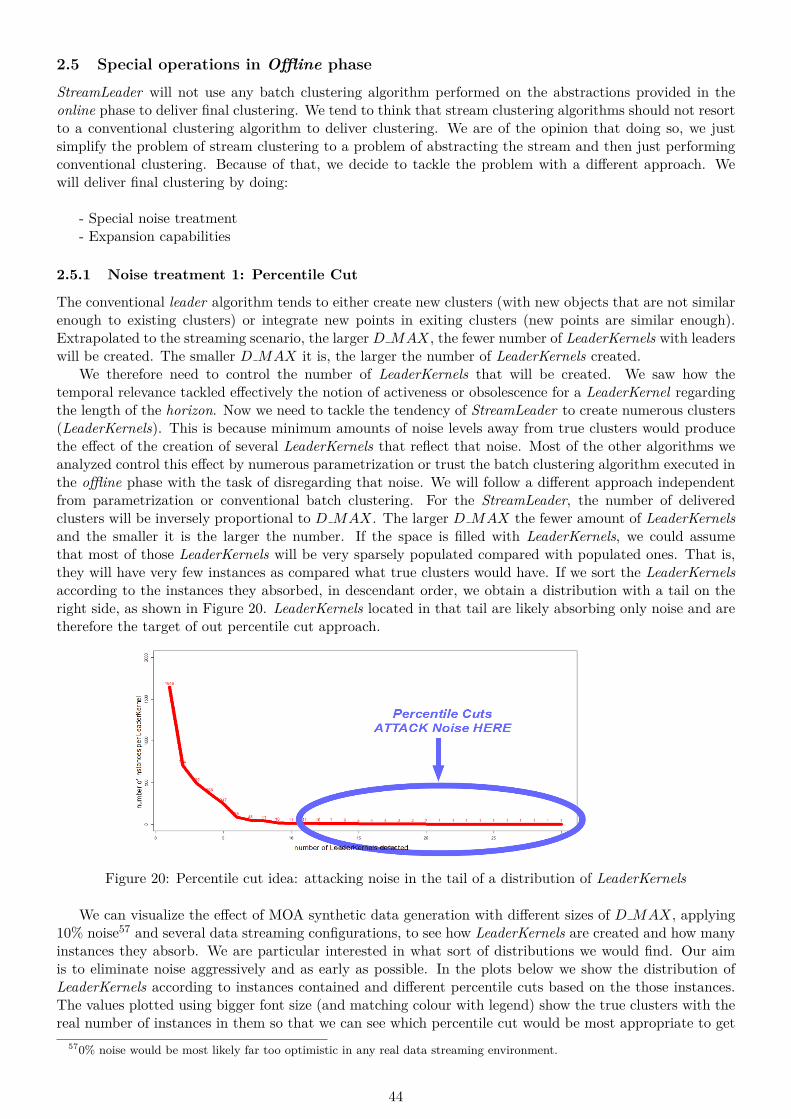
2.5 Special operations in Offline phase

StreamLeader will not use any batch clustering algorithm performed on the abstractions provided in theonline phase to deliver final clustering. We tend to think that stream clustering algorithms should not resortto a conventional clustering algorithm to deliver clustering. We are of the opinion that doing so, we justsimplify the problem of stream clustering to a problem of abstracting the stream and then just performingconventional clustering. Because of that, we decide to tackle the problem with a different approach. Wewill deliver final clustering by doing:

- Special noise treatment- Expansion capabilities

2.5.1 Noise treatment 1: Percentile Cut

The conventional leader algorithm tends to either create new clusters (with new objects that are not similarenough to existing clusters) or integrate new points in exiting clusters (new points are similar enough).Extrapolated to the streaming scenario, the larger D MAX, the fewer number of LeaderKernels with leaderswill be created. The smaller D MAX it is, the larger the number of LeaderKernels created.

We therefore need to control the number of LeaderKernels that will be created. We saw how thetemporal relevance tackled effectively the notion of activeness or obsolescence for a LeaderKernel regardingthe length of the horizon. Now we need to tackle the tendency of StreamLeader to create numerous clusters(LeaderKernels). This is because minimum amounts of noise levels away from true clusters would producethe effect of the creation of several LeaderKernels that reflect that noise. Most of the other algorithms weanalyzed control this effect by numerous parametrization or trust the batch clustering algorithm executed inthe offline phase with the task of disregarding that noise. We will follow a different approach independentfrom parametrization or conventional batch clustering. For the StreamLeader, the number of deliveredclusters will be inversely proportional to D MAX. The larger D MAX the fewer amount of LeaderKernelsand the smaller it is the larger the number. If the space is filled with LeaderKernels, we could assumethat most of those LeaderKernels will be very sparsely populated compared with populated ones. That is,they will have very few instances as compared what true clusters would have. If we sort the LeaderKernelsaccording to the instances they absorbed, in descendant order, we obtain a distribution with a tail on theright side, as shown in Figure 20. LeaderKernels located in that tail are likely absorbing only noise and aretherefore the target of out percentile cut approach.

Figure 20: Percentile cut idea: attacking noise in the tail of a distribution of LeaderKernels

We can visualize the effect of MOA synthetic data generation with different sizes of D MAX, applying10% noise57 and several data streaming configurations, to see how LeaderKernels are created and how manyinstances they absorb. We are particular interested in what sort of distributions we would find. Our aimis to eliminate noise aggressively and as early as possible. In the plots below we show the distribution ofLeaderKernels according to instances contained and different percentile cuts based on the those instances.The values plotted using bigger font size (and matching colour with legend) show the true clusters with thereal number of instances in them so that we can see which percentile cut would be most appropriate to get

570% noise would be most likely far too optimistic in any real data streaming environment.

44

rid of the noise.

Figure 21 shows StreamLeader running in MOA with a setting D MAX = 0.1 at two random specificmoments in the stream analysis. Around 30 LeaderKernels are maintained and a 70th cut seem to capturethe true clusters properly:

Figure 21: Distribution of LeaderKernels according to number of instances. Percentile cuts (1)

Figure 22 represents the same sort of experiments using D MAX = 0.2 at four different instants. Nownumber of LeaderKernels is reduced to around 10 since the structures created are larger than those usingD MAX = 0.1. We see how percentile cuts behave in different distributions:

Figure 22: Distribution of LeaderKernels according to number of instances. Percentile cuts (2)

45

We observe that, if noise exists, it will be located always in the tail of the distribution. Because ofits nature, the leader approach tends to create LeaderKernels capturing the mass of the true clusters andalso the noise. We see that a specific percentile cut in each example would help reducing the true noisein the tail. In the examples above the proper cut to get rid of noise would range from 35th to 85th percentile.

While we used synthetic data generation from MOA for these examples, we noticed that the distributionof LeaderKernels based on weight (instances contained) follows an exponential-like distribution. This meansthat true clusters (and the LeaderKernels capturing them) contain most of the instances as comparedLeaderKernels capturing only noise. In order to explore the flexibility of percentile cuts, we can imaginethat the weight of LeaderKernels is, for instance, linear. Even if we can not generate this scenario in MOA,we manually create such distribution and visualize the results as shown in Figure 23:

Figure 23: Manually generated distribution of LeaderKernels. Percentile cuts (3)

If assignation of instances to LeaderKernels was to be linear, percentile cuts would still be useful withmore or less accuracy.

Lastly, we can think of the worst possible adverse scenario for the StreamLeader where the noise treatmentcould, at least, disregard the LeaderKernel with least instances. This scenario is a perfect 0% noise-freedata stream environment. In Figure 24 a view of how the percentile cut approach would approximatelywork:

Figure 24: Distribution of LeaderKernels with 0% noise. Percentile cuts (4)

46

With exactly 0% noise, there would be no tail to be cut because there is no noise. Very low percentilecuts should be applied and at least, last LeaderKernel would be lost. In the left example above, the Lead-erKernel with 18 instances would be discarded. In the right one, a LeaderKernels with 540 instances wouldbe disregarded. This situation could occur but could be handled. Still, with just one instance appearing asnoise, tail would exist again.

By knowing the behavior of percentile cuts based on the examples above, the uncertainty in noise lev-els (most likely above 0%) and the role the parameter D MAX plays, we decide to be conservative, applya 45% percentile cut to remove noise in the tail, and leave the rest of potential non-removed noise to thesecond noise treatment (explained in next section). We should not confuse a cutting point below 45thpercentile in distribution of LeaderKernels with an stream containing 45% noise. The aim of the cut is toremove LeaderKernels that are capturing just noise in the stream, i.e. 5%, 20%, 40% or any. Whateveramount of noise there is, there will be always LeaderKernels capturing it (Hartigan’s Leader concept willalways fill the space with clusters as long as an instance appears where no other cluster already exists).Similarly StreamLeader will fill the d-space with LeaderKernels where noise appears. If noise is sparse ind-space, then many LeaderKernels will be created to fill those regions in space. On the other hand, if noiseis very concentrated in a region (this now sounds close to what a real clusters is), fewer LeaderKernels willfill that particular region. In either of the two scenarios, several LeaderKernels with noise are created andmost likely placed in the tail. Most likely scenario is to have many noisy LeaderKernels. A 45th percentilecut is flexible enough to remove many of them if necessary, but not as aggressive as to remove many properLeaderKernels when the tail is not that long containing scattered noise. Worst case would be having noisyLeaderKernels having more weight than the real clusters themselves, but then it would not be noise, it wouldbe a true cluster.

The part of the pseudo-code dealing with this noise treatment is as follows:

(L List of LeaderKernels)

53 L← Sort(L) in descending order according to weight of each LeaderKernel

55 perc threshold← 45 percentile on distribution of L according to LeaderKernel’s weight56 traverse l ∈ L and remove l with weight(l) < perc threshold

47

2.5.2 Noise treatment 2: Logarithmic Cut

Percentile cuts are useful for cutting tails in distributions and this is where noise would appear. However,situations could also occur when the cuts do not eliminate completely LeaderKernels with few instanceswhich we would otherwise consider as noise. We therefore develop an additional strategy to get rid ofpotential noise that could be located on the elbow of the distribution, as Figure 25 shows.

Figure 25: Logarithmic cut idea: attacking noise in the elbow of a distribution of LeaderKernels

We will basically try to estimate on-the-fly what few could be in the current data stream. We exploitagain the sorted distribution of LeaderKernels and assume that, if there are still some in the tail representingnoise, the amount of instances they contain would be in the around an order of magnitude smaller than theLeaderKernels representing the largest true cluster.

We show examples of scenarios with the situations described above. We apply percentile cuts to distri-butions based on LeaderKernels and finally several logarithmic cuts representing the concept of orders ofmagnitude. First two scenarios with D MAX = 0.1 and 10% noise show in Figure 26. We can observe onthe left plots, that numerous LeaderKernels are created with few instances (located in the tail). The plotsin the center show the remaining distribution after applying a percentile cut, where a substantial number ofnoise has been eliminated. The plots on the right show the cut-off locations using different base logarithms.In both scenarios (upper and bottom plots) with many LeaderKernels in the distribution, a cut-off pointsbase 1.1 logarithms would be too aggressive, eliminating LeaderKernels representing true clusters.

48

Figu

re26

:Lo

garit

hmic

cuts

ondi

strib

utio

nof

Lead

erK

erne

lsw

ithDMAX

=0.

1,w

ith10

%no

ise

49

Figure 27 shows StreamLeader with a setting of D MAX = 0.2 and 10% noise, which implies a creationof fewer number of LeaderKernels than by using 0.1. With fewer clusters, we should be careful not toeliminate valid ones located in the elbow of the distribution. A conservative approach in these situationsis therefore the choice of a lower base logarithm, since basis 1.1 is again too aggressive. Basis 1.3 seemsconservative enough.

Figure 27: Logarithmic cuts on distribution of LeaderKernels with D MAX = 0.2, 10% noise

As with percentile cuts, we would like to check logarithmic cuts in a distribution with constant slope(different from exponential-like). Since we can not create such scenario in MOA, we emulate manually thedistribution. Figure 28 shows two of such situations. In the top plots, upper left shows a distribution ofLeaderKernels based on weight. In the upper center, the distribution after performing 45th percentile cut.On the upper right, the different cut points in the distribution applying different logarithms. Base 1.1would be too aggressive by eliminating the LeaderKernel with 35 instances, which is a true cluster. Higherbasis cut would not cut any of the true clusters. Bottom plots present another situation, with bottom leftpresenting a LeaderKernel with 70000 instances, a small set of true LeaderKernels 35 to 300 instances each,and lastly LeaderKernels capturing noise with 1 to 9 instances. Bottom middle pot shows the distributionafter performing 45th percentile, which has eliminated noisy LeaderKernels of up to 35 instances weight.Bottom right shows where cuts would be executed using the different logarithms. Due to the magnitude ofthe 70000 weight LeaderKernel we see them all together. The cut-off values would be 117 for basis 1.1, 42for basis 1.3, 27 for basis 1.5, 21 for basis 1.7, 5 for basis 10. Basis 1.1 is too aggressive, being basis 1.3 theone that removes noise better without eliminating LeaderKernels representing true clusters.

50

Figure 28: Logarithmic cuts on linear slope distribution of LeaderKernels with D MAX = 0.1, 10% noise

With the situations described above, and having in mind that a stream will always be unexpectedin behavior, we estimate that treating noise as if it was orders of magnitude smaller than true clustersis a reasonable solution. The aim is to use it as complementary technique to eliminate any remainingLeaderKernel that was not eliminated with the percentile cuts. From all the bases used in the scenarios, 1.3seems a sensible choice, which eliminates noise and respects true clusters in most of the cases. Even withthe large 70000 cluster and several small ones, only one true cluster with 35 instances would be incorrectlydiscarded.

As commented before, we are attempting to aggressive remove noise in a flexible way so we are notdependent on the use of conventional clustering and/or specialized parametrization. The two techniquescombined and applied sequentially (percentile and logarithmic cut) make use of the distribution of Stream-Leaders by attacking the noise in the tail first and then in the elbow of the distribution. They try toconfer StreamLeader as much flexibility as possible to handle very diverse scenarios where noise and clusterscould be presented in different ways, i.e. strong noise or weak, massive clusters only, combination of mas-sive and sparsely populated plus noise and so on. The pseudo-code addressing noise though logarithmic cuts:

(L List of LeaderKernels)

53 L← Sort(L) in descending order according to weight of each LeaderKernel

57 log biggest lk ← log base 1.3 of weight of first LeaderKernel with more instances58 traverse l ∈ L and remove l with weight(l) < log biggest lk

51

2.5.3 Expansion of intersecting LeaderKernels with radius D MAX

D MAX is the only parameter needed by the algorithm. It expresses the guidelines given by the userregarding how much proximity the instances should have in order to cluster them together (resulting inbigger or smaller clusters). We gave LeaderKernels the capability to contract according to the size of massdetected. This overrides D MAX by adapting as much as possible to the structures perceived. However,there could also be situations where we want to override by expanding to a new cluster size that D MAXcan not fully capture. We will therefore allow the expansion of a LeaderKernel when we detect severalLeaderKernels with maximum radius D MAX that are overlapping. This is a good indication that themass to capture requires a bigger radius.

In Figure 29, on the left side, we detect three LeaderKernels with radiusD MAX, being LK0 the one withlargest mass or number of instances absorbed. Then we look for potential LeaderKernels with also radiusD MAX that overlap with LK0 by checking if distances 58 between respective leaders is < (D MAX ∗ 2).In the middle, we observe how farthest distance to neighboring leaders is determined. This distance wouldindicate that, from leader of the LeaderKernel with most weight (Leader0) to the extreme of the farthestaway LeaderKernel (LK1), the hyper-sphere with that distance as radius would most likely cover all over-lapping LeaderKernels in space. On the right side, the LeaderKernel with largest mass will absorb itsneighbors and will have its mass and statistical summarizations updated (Property 2, additivity), showingas (LK0′). It will be set as artificially expanded, and an new artificial radius will be approximated (125%farthest dist between leaders + D MAX), overriding D MAX. 25% accounts for approximations due tothe fact that we work always with summarized data. It is worth noticing that the leader Leader0′ repre-senting LK0′ will not coincide with any of leaders Leader0, Leader1 or Leader2 that represented LK0, LK1and LK2 respectively before the expansion process took place.

Figure 29: Intersecting LeaderKernels with radius D MAX (left) merge into one bigger LeaderKernel (right)

58Distance function we defined in former sections.

52

A limit in the amount of growth is imposed. Since we work in normalized space and we still want touse user-defined D MAX as a reference, we set an upper limit of 60% the value of original D MAX. Thisshould be seen as the amount of automatic flexibility we give to StreamLeader once D MAX has beenspecified. It is of course possible that the cluster is still of bigger size. In that case, several LeaderKernelswill try to capture its mass, but always limited to the 60% threshold59.

The pseudo-code corresponding to this expansion is the following:

5 Expand Factor Max← 60 percent7 Radius Expand Max← increase D MAX by Expand Factor Max

59 lk max← LeaderKernel radius D MAX and largest weight60 lks Engolf ← LeaderKernels with radius D MAX with leader at distance < (D MAX ∗ 2)

from leader of lk max61 farthest dist between leaders← max distance between leader of lk max and leaders of lks Engolf62 for lk engolfed ∈ lks Engolf do63 lk max← lk max ∪ lk engolfed64 L← L− lk engolfed65 end for66 if farthest dist between leaders > 0 then67 setArtifitiallyExpanded(lk max)68 newRadius← 125% farthest dist between leaders+D MAX69 if newRadius < Radius Expand Max then70 setArtifitiallyExpandedRadius(lk max, newRadius)71 else72 setArtifitiallyExpandedRadius(lk max,Radius Expand Max)73 end if74 end if

2.5.4 Expansion of LeaderKernels with radius D MAX

There could be also situations where a LeaderKernel with radius D MAX can not capture fully a clusterbut it senses that more mass is surrounding it in the d-dimensional space. Such situation is represented inFigure 30:

Figure 30: One (non overlapping) LeaderKernel with radius D MAX (left) expands its radius (right)

We recall that LeaderKernels have the tendency to contract to smaller size when µ distance to leader ofinstances absorbed is less than 80% of half of D MAX (LSDN < (D MAX

2 ∗0.8)). If we detect a LeaderKernel59Additional expansion processes will be explained in next sections.

53

with maximum radius D MAX, it means that it did not find the need to contract to a smaller appropriateradius. On the other hand, it is quite likely that more mass can be found in the surrounding space. TheLeaderKernel is therefore given the chance to expand, not to the maximum allowed of 60% increase overD MAX, but to an intermediate size of 30% increase. None of the summarized statistics are updated(including the leader Leader1), only the new radius is assigned and LK1 is set as artificially expanded. Thiswill override the behavior of the LeaderKernel to return artificial radius and not D MAX. It is also worthnoticing that if such LeaderKernel is found, it is most likely isolated and not overlapping with others ofD MAX radius in space. Otherwise it would have merged with its neighbors as we explained in the firstexpansion method. Lastly, it is worth noticing that a situation could arise where a LeaderKernel was justcreated with automatic radius of size D MAX and had no time to contract because it did not absorbedinstances yet. In order to avoid that situation, we will expand only those with a creation date happeningbefore 1

4 th the duration of the horizon counting back from current time. We do this in order to make surethat they had some time units available to capture instances and had time to contract if needed.

Below the corresponding pseudo-code:

4 Expand Factor Min← 30 percent6 Radius Expand Min← increase D MAX by Expand Factor Min

75 expand t threshold← timestamp− (H/4)76 lks ExtraRadius← LeaderKernel radius D MAX and creation date < expand t threshold77 for lk expand ∈ lks ExtraRadius do78 setArtifitiallyExpanded(lk expand)79 setArtifitiallyExpandedRadius(lk expand,Radius Expand Min)80 end for

2.5.5 Expansion of intersecting LeaderKernels with radius artificially expanded

There is a third situation where LeaderKernels might want to expand in size. The first two expansionprocesses took D MAX LeaderKernels and produced another one with larger radius. In both cases, theresulting LeaderKernel was set as artificially expanded (meaning that user guideline D MAX was overriddenas radius). First process allowed a maximum expansion of 60% of original D MAX, and, if not reachingthat, to the estimated size according to the mass detected. The second process produced an expansionto a factor of 30% of original D MAX, producing a LeaderKernel which is likely isolated in space andcovers hopefully most of the true cluster. However, it is also possible that the second expansion was due tonon-overlapping LeaderKernels that, together were trying to cover one unique cluster of much bigger size.

If the expansion succeeded, then the chances that overlapping now occurs are increased (otherwise theone LeaderKernels will remain isolated). If we detect it, then we proceed again with a merging process,allowing again to a maximum of 60% expansion ratio of original D MAX.

Figure 31 shows in the left side three LeaderKernels with radio D MAX, each covering a portion of d-dimensional space where high concentration of instances are located. They do not overlap, therefore, shownon the right, they are each artificially expanded (as explained in second type of expansion processes). A newradius of size 30% bigger than D MAX is allocated to each one in the hope that they capture the clusterbetter. We should notice that when these expansions occur, the leaders do not change, only the radius areincreased in sized (as opposed to merging where leaders are recalculated because of the new statistics ofthe involved LeaderKernels). The LeaderKernel with more weight (in this case LK2) and the overlappingneighbors (LK0 and LK1) are detected. This is done by checking the distances between pairs of leaders. Ifthey overlap, then the distance is less than ((130% D MAX) ∗ 2)60.

Finally, Figure 32 shows the last two steps to finish the expansion process. On the left, farthest distancebetween leaders is found. The one with more mass absorbs the others (by additive property of a LeaderK-ernel), the rest are discarded, and radius is calculated by adding the one they had to the farthest distancebetween leaders with a 25% increase fluctuation factor61 to correct for approximations of a streaming envi-

6030% increase over D MAX is the amount of expansion flexibility we give to StreamLeader in the context of a normalizedd-dimensional space and should not be mistaken with an input parameter.

61Again, this is an informed amount of flexibility we add in order to compensate for approximations in the streamingenvironment.

54

Figure 31: Three non overlapping LeaderKernels of radius D MAX (left) expand radius and overlap (right)(1)

ronment. Again, if the new radius trespasses the 60% maximum expansion threshold, then that threshold ismaintained. Otherwise the radio is the result of the calculation (125% farthest dist between radius+130%D MAX). On the right, after the merging completes, the one LeaderKernel remains, its leader is placedin space according to the statistics of the combined LeaderKernels, and the new radius tries to cover morespace than before the start of the process62.

Figure 32: Three overlapping and expanded LeaderKernels (left) merge into a bigger one (right) (2)

62As we will see in the StreamLeader workflow algorithm, D MAX is still used as area of influence for attracting new instances.The difference is that MOA will use this new calculated radius, and not D MAX, in order to check whether the output ofthe algorithm matches the ground-truth or the true clusters. This will be done by checking to which cluster is each instanceallocated, and it will be possible by using the GET INCLUSION PROBABILITY function we defined for the LeaderKernels.

55

Below the corresponding pseudo-code:

4 Expand Factor Min← 30 percent5 Expand Factor Max← 60 percent6 Radius Expand Min← increase D MAX by Expand Factor Min7 Radius Expand Max← increase D MAX by Expand Factor Max

81 lk max← LeaderKernel with radius Radius Expand Min and largest weight82 lks Engolf ← LeaderKernels with radius Radius Expand Min

with leader at distance < (Radius Expand Min ∗ 2) from leader of lk max83 farthest dist between leaders← max distance between leader of lk max and leaders of lks Engolf84 for l engolfed ∈ lks Engolf do85 lk max← lk max ∪ l engolfed86 L← L− l engolfed87 end for88 if farthest dist between radius > 0 then89 setArtifitiallyExpanded(lk max)90 newRadius← 125% farthest dist between radius+Radius Expand Min91 if newRadius < Radius Expand Max then92 setArtifitiallyExpandedRadius(lk max, newRadius)93 else94 setArtifitiallyExpandedRadius(lk max,Radius Expand Max)95 end if96 end if

56

2.6 Pseudocode

We have already defined LeaderKernels, properties and operations as individual pieces. We will use them togenerate statistical abstraction and adaptation to the dynamic data stream. On the other hand, we have alsodefined processes to carry out in the offline phase. They focus on aggressive noise treatment and expansioncapabilities to describe better the discovered clusters, and they will be needed in order to compensate fornot using any conventional clustering algorithm that take the abstractions as input (as most of other streamapproaches do). In this section we can find first the proximity measure used. Then full pseudo-code relatedto LeaderKernel. Finally we will present our new stream clustering algorithm, called StreamLeader.

2.6.1 Proximity measure

DISTANCE FUNCTION:

FUNCTION: DISTSLINPUT: I1, I2 stream data instances in d-dimensional space (or any object in that same d-dimensionalspace, like a leader representing a LeaderKernel)OUTPUT: D distance between the two given instances I1, I2

1 d← dimensionality of I12 D ←

√∑di=1(I1

i − I2i )2

3 D ← DD+1

4 return D

2.6.2 LeaderKernel

ATTRIBUTES:

LS : vector of d entries.For each dimension, linear sum of all the instances added to the LeaderKernel. The p-th entry of LS is equalto

∑nj=1 x

jp.

- SS : vector of d entries.For each dimension, squared sum of all the instances added to the LeaderKernel. The p-th entry of SS isequal to

∑nj=1(xjp)2.

- LST : linear sum of the timestamps of all instances added to the LeaderKernel, equal to∑nj=1 T

j .

- SST : squared sum of the timestamps of all instances added to the LeaderKernel, equal to∑nj=1(T j)2.

- LSD: linear sum of the distances to the leader of all instances added to the LeaderKernel, equal to∑nj=1D

j .

- D MAX : influence of the LeaderKernel, taken its leader as representative, in its neighborhood in thenormalized d-dimensional space, measured in terms of the distance function DISTSL, with range (0...0.5].

- N : Number of instances added to the LeaderKernel.

- creation timestamp: timestamp that indicates when the LeaderKernel was created.

- is artificially expanded: boolean that indicates whether the LeaderKernel was artificially expanded far-ther than indicated by D MAX.

- artificially expanded radius: radius of the LeaderKernel as a result of an artificial expansion process.

57

CONSTRUCTORS (INSTANCE & CLUSTER BASED):

PROCEDURE: CREATEINSTANCE BASED

INPUT: I stream data instance, d dimensions, TS timestamp for addition of I to LeaderKernel, DMAXradio of influence of this LeaderKernel, TSTMP creation timestamp for creation of LeaderKernelOUTPUT: ∅

1 N ← 12 LS ← I on each dimension3 SS ← I2 on each dimension4 D MAX ← DMAX5 LST ← TS6 SST ← TS2

7 creation timestamp← TSTMP creation8 LSD ← 09 is artificially expanded← false10 artificially expanded radius← 0

PROCEDURE: CREATECLUSTER BASED

INPUT: lk LeaderKernel, DMAX radio of influence around this LeaderKernel, TSTMP creation creationtimestamp, AER artificially expanded radius assigned to LeaderKernel, WAE boolean indicating whetherthe LeaderKernel was artificially expanded farther than indicated by D MAXOUTPUT: ∅

1 N ← num instances contained in lk2 LS ← LS of lk3 SS ← SS of lk4 D MAX ← DMAX5 LST ← LST of lk6 SST ← SST of lk7 LSD ← LSD of lk8 creation timestamp← TSTMP creation9 is artificially expanded←WAE10 artificially expanded radius← AER

58

INSERT INSTANCE:

PROCEDURE: INSERT INSTANCEINPUT: I stream data instance, TS timestamp for addition of I to LeaderKernel, i DTL distance from Ito leader representing this LeaderKernelOUTPUT: ∅

1 N ← N + 12 LST ← LST + TS3 SST ← SST + TS2

4 LS ← LS + I on each dimension5 SS ← SS + I2 on each dimension6 LSD ← LSD + i DTL

GET LEADER:

FUNCTION: GET LEADERINPUT: ∅OUTPUT: L as statistical center of the LeaderKernel in d-dimensional space

1 L← LSN on each dimension2 return L

MERGE (LeaderKernels):

PROCEDURE: MERGEINPUT: lkadd LeaderKernel to be absorbedOUTPUT: ∅

1 radius← get radius2 radius lk ← get radius from lkadd3 creation timestamp lk ← get creation timestamp in lkadd4 N lk ← num instances contained in lkadd5 LS lk ← LS in lkadd6 SS lk ← SS in lkadd7 LST lk ← LST contained in lkadd8 SST lk ← SST contained in lkadd9 LSD lk ← LSD contained in lkadd10 is artificially expanded l← check if lkadd was artificially expanded11 creation timestamp← if N 6= 1, creation timestamp, otherwise creation timestamp lk 12 N ← N + N lk13 LST ← (N∗LST )+(N lk∗LST lk)

(N+N lk)

14 SST ← (N∗SST )+(N lk∗SST lk)(N+N lk)

15 LSD ← (N ∗ LSD) + (N lk ∗ LSD lk)16 is artificially expanded← is artificially expanded or is artificially expanded lk17 artificially expanded radius← max between radius and radius lk18 LS ← LS + LS lk19 SS ← (N∗SS)+(N lk∗SS lk)

(N+N lk)

59

HANDLING TIME:

FUNCTION: GET CREATION TIMEINPUT: ∅OUTPUT: TS creation timestamp

1 TS ← creation timestamp2 return TS

FUNCTION: GET µ TIMEINPUT: ∅OUTPUT: TS timestamp representing the arrival mean time of all instances contained in the LeaderKernel

1 TS ← LSTN

2 return TS

FUNCTION: GET σ TIMEINPUT: ∅OUTPUT: TS timestamp representing the standard deviation of the arrival timestamps of all instancescontained in the LeaderKernel

1 TS ←√

SSTN − (LSTN )2

2 return TS

FUNCTION: GET RELEV ANCE STAMPINPUT: ∅OUTPUT: TS temporal relevancy timestamp of the entire LeaderKernel

1 MuTime← get µ Time2 SigmaTime← get σ Time3 if not is artificially expanded then4 TS ←MuTime + SigmaTime5 else6 TS ← MuTime7 return TS

HANDLING DISTANCE:

FUNCTION: GET µ DISTANCE TO LEADERINPUT: ∅OUTPUT: D average distance to the leader representing the LeaderKernel (of all distances of all instancesto leader at the time they were added to the LeaderKernel)

1 D ← LSDN

2 return D

FUNCTION: GET RELEV ANT DISTANCE TO LEADERINPUT: ∅OUTPUT: D distance

1 D ← get µ Distance to leader2 return D

60

FUNCTION: GET RADIUSINPUT: ∅OUTPUT: R radius of the LeaderKernel

1 Mu D ← get µ distance to leader2 R← 03 if not is artificially expanded then4 if Mu D < (D MAX

2 ∗ 0.8) then R←Mu D ∗ 25 else R← D MAX6 end if7 else R← artificially expanded radius8 end if9 return R

ARTIFICIAL EXPANSION:

PROCEDURE: SET ARTIFICIALLY EXPANDEDINPUT: IAE boolean indicating whether the LeaderKernel is artificially expandedOUTPUT: ∅

1 is artificially expanded← IAE

PROCEDURE: SET ARTIFICIALLY EXPANDED RADIUSINPUT: AE Radius artificially expanded radius to be assigned to this LeaderKernel (overrides D MAXas radius)OUTPUT: ∅

1 artificially expanded radius← AE Radius

INCLUSION PROBABILITY:

FUNCTION: GET INCLUSION PROBABILITYINPUT: I stream data instanceOUTPUT: P probability of I belonging to this LeaderKernel

1 L← leader of this LeaderKernel2 R← radius of this LeaderKernel3 D ← DISTSL between L and I4 if D ≤ R then return 15 else return 0

61

LIDERKERNEL COMPARISON:

FUNCTION: IS SAME LeaderKernelINPUT: lk LeaderKernelOUTPUT: I S LK boolean stating whether the LeaderKernel provided as input parameter is the same asthis instance of the class

1 N lk ← num instances contained in lk2 LS lk ← LS in lk3 SS lk ← SS in lk4 LST lk ← LST contained in lk5 SST lk ← SST contained in lk6 LSD lk ← LSD contained in lk7 creation timestamp lk ← creation timestamp in lk8 is artificially expanded lk ← check if lk was artificially expanded9 radius← get radius10 radius lk ← get radius from lk11 I S LK ← (N = N lk and LS = LS lk and SS = SS lk and LST = LST lk and

SST = SST lk and LSD = LSD lk andcreation timestamp = creation timestamp lk andis artificially expanded = is artificially expanded lk and radius = radius lk)

12 return I S LK

ACCESS ATTRIBUTES:

FUNCTION: GET LSINPUT: ∅OUTPUT: LS vector of d entries. For each dimension, linear sum of all the instances added to the Lead-erKernel

1 return LS

FUNCTION: GET SSINPUT: ∅OUTPUT: SS vector of d entries. For each dimension, squared sum of all the instances added to theLeaderKernel

1 return SS

FUNCTION: GET LSTINPUT: ∅OUTPUT: LST linear sum of the timestamps of all instances added to the LeaderKernel

1 return LST

FUNCTION: GET SSTINPUT: ∅OUTPUT: SST squared sum of the timestamps of all instances added to the LeaderKernel

1 return SST

62

FUNCTION: GET LSDINPUT: ∅OUTPUT: LSD linear sum of the distances to the leader of all instances added to the LeaderKernel

1 return LSD

FUNCTION: GET DMAXINPUT: ∅OUTPUT: D MAX influence of the LeaderKernel, taken its leader as representative, in its neighborhood inthe normalized d-dimensional space, measured in terms of the distance function DISTSL, with range (0...0.5].

1 return D MAX

FUNCTION: GET NINPUT: ∅OUTPUT: N Number of instances added to the LeaderKernelObservation: Because LeaderKernel extends CFCluster class in MOA, this function is also available asGET WEIGHT.

1 return N

FUNCTION: GET CREATION TIMESTAMPINPUT: ∅OUTPUT: creation timestamp timestamp that indicates when the LeaderKernel was created.

1 return creation timestamp

FUNCTION: IS ARTIFICIALLY EXPANDEDINPUT: ∅OUTPUT: is artificially expanded: boolean that indicates whether the LeaderKernel was artificially ex-panded farther than indicated by D MAX.

1 return is artificially expanded

FUNCTION: ARTIFICIALLY EXPANDED RADIUSINPUT: ∅OUTPUT: artificially expanded radius: radius of the LeaderKernel as a result of an artificial expansionprocess.

1 return artificially expanded radius

63

2.6.3 StreamLeader

This section contains the pseudo-code describing the behavior of the StreamLeader, which is the completestream clustering algorithm. It respects the general concept of the leader approach. We show first a flowchart with the summarization of the algorithm. Then a high-level version pseudo-code with the main tasksexecuted. Then a lower-level one with further details.

First, a flow chart with graphic icons associated with each task is shown in Figure 33:

Figure 33: Flow chart of the StreamLeader algorithm

64

The algorithm requires one single parameter, D MAX. It indicates the area of influence that a leader,as representative of its LeaderKernel, has in the multi-dimensional space 63. We need to assign a defaultvalue that gives StreamLeader high flexibility overall, in any stream clustering scenario.

While reviewing the literature and the different algorithms, we find no homogeneous way in whichdefault parametrization is chosen by the authors. Backing the choice with theoretical results does notseem a standard process. Instead, default parametrization is either advised by the authors or backed byexperimental results obtained using specific data sets. Since a data stream is dynamic in nature and thedata generation processes for those data sets can evolve, we prefer to base our choice not with experimentsbut with reasoning based on the key characteristics of StreamLeader. In that way, in order to decide onthat value there are some factors to consider. StreamLeader works in d-dimensional space restricted to[0,1]. That means, biggest single hyper-spherical cluster covering maximum d space (reach max values ineach dimension) would be radius = 0.5. We will not find that clustering problem normally, because almostevery instance would be similar to any other, all falling in the same cluster. Two clusters with half of themaximum radius would be still considerably big size clusters, with radius = 0.25, which would be collidingin space as soon as there is a minimum of concept drift and movement of true clusters. Considering thatLeaderKernels can contract to any smaller size, it is logical to think that we should make sure that itsexpansion capabilities are enough to capture a bigger (but not far bigger) true cluster of what D MAXindicates. This is needed in order to avoid situations where many LeaderKernels try to capture a single truecluster.

A reasonable cluster size to cover using default parametrization would be around 70% of such clusterof radius = 0.25. That is, we need our LeaderKernels to be able to expand to a radius of 0.25 ∗ 0.7 =0.175. Because LeaderKernels can expand a maximum factor of 60% of D MAX, then LeaderKernels withD MAX = 0.11 could reach to a radius 0.11∗1.6 = 0.176, which is the maximum radius size true cluster wewant to capture properly (using just one LeaderKernels) using default parametrization, in d space [0,1]. Tovisualize the above mentioned cluster sizes in dimensions of size restricted to [0,1], we can see in Figure 34a true cluster with maximum radius = 0.5 (left), two clusters of radius = 0.25 (middle) and finally a truecluster of radius = 0.176. Any cluster of radius smaller than 0.176 can be captured thanks to contractioncapabilities.

Figure 34: Cluster maximum radius 0.5 (left), two of radius 0.52 = 0.25 (middle) and one 70% 0.5

2 = 0.176

D MAX < 0.11 it is also possible, but then we would have less changes of capturing bigger clusterswith one unique LeaderKernel. Using several to detect a single true cluster would cause drops in qualitymeasures like Completeness, Rand Statistics, etc. Figure 35 visualizes the problematic of covering a biggertrue cluster of radius = 0.176 with several small LeaderKernels with D MAX = 0.06.

63Window Size or Horizon is also a parameter, but not related to the algorithm but to the kind of analysis the user wants tocarry out, in the sense that all stream clustering algorithms that use with time window models need it.

65

Figure 35: Clustering quality drops when a true cluster is covered by several smaller sized LeaderKernels

D MAX > 0.11 it is possible as well, but then problems would arise in streaming scenarios where smallsize clusters are present. One single LeaderKernel would likely capture groups of several small true clusters,just because their masses fall within D MAX range. This would penalize again Recall, Homogeneity, andother measures. Figure 36 shows a group of smaller size true clusters, radius in range 0.015 to 0.45, beingcaptured by a single LeaderKernel with larger D MAX = 0.13.

Figure 36: Clustering quality drops when several true clusters are captured by a single LeaderKernels withtoo large D MAX

So D MAX = 0.11 is a trade-off, between ability to capture a bigger single true cluster with just oneLeaderKernel using expansion capabilities (and avoiding the use of several to capture its mass) and capturinga single small true cluster with a single LeaderKernel (and avoiding capturing several with one oversizedLeaderKernel). Again, D MAX should be understood as a user guideline regarding the size of structuresthe user wants to detect, or how low or high-level granularity in the data we want to isolate. StreamLeadertries to adapt that guideline, within certain limits, to the reality of the data distributions.

66

HIGH-LEVEL PSEUDO-CODE

INPUT: H time window, D MAX radio of influence of each leader in normalized spaceOUTPUT: L List of LeaderKernels describing the clusters in the data stream relevant in the horizon

1 Initialize variables2 while DATA STREAM ACTIVE do3 Take incoming instance4 if First instance ever then5 Create new LeaderKernel with instance6 else7 Try integrate instance in existing LeaderKernel8 if No integration then9 Create new LeaderKernel with instance10 end if11 end if12 if Overlapping current LeaderKernel with existing one then13 Merge current LeaderKernel with existing one14 end if15 Phase out old LeaderKernels16 LeaderKernel Sorting in descendant order according to weight17 if Current time window completes then18 Percentile cut on distribution of LeaderKernels according to weight19 Logarithmic cut on distribution of LeaderKernels according to weight20 Merge intersecting LeaderKernels of radius D MAX and expand up to maximum ratio21 Expand LeaderKernels with radius D MAX to minimum expansion ratio22 Merge intersecting LeaderKernels expanded to minimum ratio and expand up to maximum23 Deliver L to MOA for cluster evaluation24 end if25 end while

67

LOW-LEVEL PSEUDO-CODE

INPUT: H time window, D MAX radio of influence of each leader in normalized spaceOUTPUT: L List of LeaderKernels describing the clusters in the data stream relevant in the horizon

1 L← ∅ (INITIALIZATION OF VARIABLES)2 timestamp← pre-start sequence at zero3 initialized leader ← false4 Expand Factor Min← 30 percent5 Expand Factor Max← 60 percent6 Radius Expand Min← increase D MAX by Expand Factor Min7 Radius Expand Max← increase D MAX by Expand Factor Max8 while instance 6= ∅ do (WHILE DATA STREAM ON)9 I ← instance10 Increase timestamp in one time unit11 dim← Dimensionality of I12 P instance← no LeaderKernel found13 noMerged← true14 noPhasedOut← true

(INSERTION OF FIRST INSTANCE EVER)15 if not initialized leader then16 L← L ∪ new LeaderKernel with I, radius D MAX, and timestamp17 P instance← newly added LeaderKernel18 initialized leader ← true19 end if

(INTEGRATION OF INSTANCE IN EXISTING LIDERKERNEL)20 J ← 021 while l ∈ L and P instance = no LeaderKernel found do22 dist ← DISTSL (I, leader of LeaderKernel l)23 if dist ≤ D MAX then24 P instance ← J25 l← l ∪ I at timestamp at distance dist 26 end if27 increase J28 end while

(CREATION OF NEW LIDERKERNEL)29 if P instance = no LeaderKernel found then30 L← L ∪ new LeaderKernel with I, radius D MAX, and timestamp31 P instance ← position of newly added LeaderKernel32 end if

(MERGING OF CURRENT LIDERKERNELWITH EXISTING ONE)33 if P instance 6= no LeaderKernel found then34 if number LeaderKernels ≥ 2 then35 l merge ← LeaderKernel at position P instance36 while l ∈ L and noMerged and l 6= l merge do37 dist ← DISTSL (leader of l merge, leader of l)38 if dist ≤ D MAX then39 l merge← l merge ∪ l40 L← L− l41 noMerged← false42 end if43 end while44 end if45 end if

(PHASING OUT OF OLD LIDERKERNELS)46 time threshold← timestamp−H47 while l ∈ L and noPhasedOut do48 if TimeRelevance(l) < time threshold then49 L← L− l50 noPhasedOut← false51 end if52 end while

68

(SORTING OF LIDERKERNEL ACCORDING TO WEIGHT)53 L← Sort(L) in descending order according to weight of each LeaderKernel

54 if timestamp module H = 0 then (CURRENT TIME WINDOW COMPLETES)

(NOISE PERCENTILE CUT)55 perc threshold← 45 percentile on distribution of L according to LeaderKernel’s weight56 traverse l ∈ L and remove l with weight(l) < perc threshold

(NOISE LOGARITHMIC CUT)57 log biggest lk ← log base 1.3 of weight of first LeaderKernel with more instances58 traverse l ∈ L and remove l with weight(l) < log biggest lk

(EXPANSION OF INTERSECTING LIDERKERNELS WITH RADIUSD MAX)59 lk max← LeaderKernel radius D MAX and largest weight60 lks Engolf ← LeaderKernels with radius D MAX with leader at distance < (D MAX ∗ 2)

from leader of lk max61 farthest dist between leaders← max distance between leader of lk max and leaders of lks Engolf62 for lk engolfed ∈ lks Engolf do63 lk max← lk max ∪ lk engolfed64 L← L− lk engolfed65 end for66 if farthest dist between leaders > 0 then67 setArtifitiallyExpanded(lk max)68 newRadius← 125% farthest dist between leaders+D MAX69 if newRadius < Radius Expand Max then70 setArtifitiallyExpandedRadius(lk max, newRadius)71 else72 setArtifitiallyExpandedRadius(lk max,Radius Expand Max)73 end if74 end if

(EXPANSION OF LIDERKERNELS WITH RADIUSD MAX)75 expand t threshold← timestamp− (H/4)76 lks ExtraRadius← LeaderKernel radius D MAX and creation date < expand t threshold77 for lk expand ∈ lks ExtraRadius do78 setArtifitiallyExpanded(lk expand)79 setArtifitiallyExpandedRadius(lk expand,Radius Expand Min)80 end for

(EXPANSION OF INTERSECTING LIDERKERNELS WITH RADIUS EXPANDED)81 lk max← LeaderKernel with radius Radius Expand Min and largest weight82 lks Engolf ← LeaderKernels with radius Radius Expand Min

with leader at distance < (Radius Expand Min ∗ 2) from leader of lk max83 farthest dist between leaders← max distance between leader of lk max and leaders of lks Engolf84 for l engolfed ∈ lks Engolf do85 lk max← lk max ∪ l engolfed86 L← L− l engolfed87 end for88 if farthest dist between radius > 0 then89 setArtifitiallyExpanded(lk max)90 newRadius← 125% farthest dist between radius+Radius Expand Min91 if newRadius < Radius Expand Max then92 setArtifitiallyExpandedRadius(lk max, newRadius)93 else94 setArtifitiallyExpandedRadius(lk max,Radius Expand Max)95 end if96 end if97 (Deliver L to MOA for cluster evaluation)98 end if99 end while100 return L

69

3 Part 3 - Testing

Once StreamLeader is integrated successfully in MOA, we put it together with Clustream, Denstream andClustree through an extensive test phase. First, we specify the computing resources available for testing.Second, we describe the metrics used for measuring quality in the results. Third, using MOA’s syntheticdata, we present the multiple test scenarios designed to test quality and sensibility for the four algorithms.Fourth, using also synthetic data, we will do extensive scalability test with different parametrization. Lastly,we will apply streaming real data and test quality results.

3.1 Computing resources used

We use a personal computer to run MOA and execute the tests. The technical specifications are the following:

- Processor: Intel(R) Core(TM) i7-3612QM CPU @ 2.10GHz- RAM: 16.0 GB- System type: 64 bits, x64- Operative system: Windows 8.1, 2013 Microsoft Corporation

3.2 Quality metrics

Here we will discuss what metrics are available for measuring quality in clustering. Also, how other streamclustering algorithms were tested. Finally, we will decide which measures we will use fr testing.

With regards to the metrics available, they can be categorized in two sets: internal or structural andexternal. Internal measures only consider cluster properties, like cluster compactness, separation betweenclusters, distances between points within one cluster or between two different, etc. On the other hand,external measures, compare the resulting clustering provided by the algorithm against an already knowntrue clustering, also known as ground-truth. This last approach takes into consideration factors like numberof clusters, size, etc.

In general, most (if not all) of the internal and external measures were designed for static scenarios andhave been used extensively in the last decades. Silhouette index [KR90], Dunn’s index [Dunn74], Sum ofSquare Distances SSQ [HK01], Root Mean Squared Standard Deviation RMSSTD [Sha96] would be someinternal measures used broadly. External measures include, among others, Entropy [SKK00], Purity [ZK04],Completeness [RH07], Homogeneity [RH07], V-measure [RH07], Precision [Rij79], Recall [Rij79], F-measure[Rij79], F1-P and F1-R in [MSE06], Variation of Information [Mei05], Mutual Information [CT06], Randstatistic [Rand71], Jaccard coefficient [FC83], Minkowsky scores [BSH+07], classification error [BSH+07],van Dongen criterion [Don00], Goodman-Kruskal coefficient [GK54], etc.

Because of the fact that streaming is a relatively new field of research, the above mentioned metricshave been also used in streaming scenarios. However, this new paradigm includes events like emerging,splitting or moving clusters, which pose a problem for conventional measures to capture them. Recently,a new evaluation measure for clustering on evolving data streams has been proposed in [KKJ+11], calledCMM, Cluster Mapping Measures, which tackles the handling of such events. It is specifically designed forstream clustering by taking important properties of evolving data steams like cluster aging, cluster joining, diminishing, etc.

Regarding to how other stream clustering algorithms were tested in terms of quality, original publica-tions of stream clustering algorithms show the use of SSQ and/or purity. This is the case of the threeStreamLeader ’s competitors in this project, namely Clustream [AHWY03], Denstream [CEQZ06] and Clus-tree [KABS11]. In streaming scenarios, SSQ takes the squared distances of the objects to the cluster centers.It has good reactions to cluster join and removal. However, it is not normalized, with unbounded upperlimit, which poses obvious problems. Purity, on the other hand, is normalized in the [0,1] range, but itdelivers fairly optimistic results when the number of clusters is large (achieving maximum purity when eachpoint gets its own cluster). Therefore measuring clustering quality in scenarios of multiple clusters is notoptimal.

70

Considering the above and metrics in MOA, we decide to take a set of seven quality measures, internaland external, and take their combined average. Since synthetic data generates labeled data, we will usepreferentially external ones. Table 5 CMM, Table 6 Rand Statistic, Table 7 Silhouette Coefficient, Table 8Homogeneity, Table 9 Completeness, Table 10 F1-P and Table 11 F1-R contain detailed descriptions of eachof the seven metrics used. Table 12 Q AVG contains the quality measure we will use for testing.

Quality Measure 1 CMM (Cluster Mapping Measures)Type External

Description

Cluster Mapping Measures are based on the concepts of connectivity between points andclusters, indicating how well a point fits the distribution of the cluster in comparison to theother points. It is a normalized sum of penalties, which includes missed points, misplacedpoints and noise inclusion. If no fault occurs, CMM returns 1 and 0 indicates maximum error.Misplaced points are calculated by mapping from clusters returned by stream clustering andground-truth.

Formulation

CMM(C,CL)64 = 1−∑

x∈Fw(x)·pen(x,C)∑

x∈Fw(x)·con(x,Cl(x))

if F = ∅, then CMM(C,CL) = 1

wherew(x): weight of an instance xpen(x,C): overall penalties for fault pointscon(x,Cli(x)): point connectivity of a point x to a cluster Ci

F : fault set, as set of objects mapped to a false classx: single instance from stream S formed by x1, ..., xN instancesC: cluster set CCL: ground-truth clustering CL

Range [0, 1]

Table 5: CMM measure details

Quality Measure 2 Rand StatisticType External

Description

It measures the percentage of decisions that are correct, measuring similarity between classesand clustering delivered. It analyzes the agreements/disagreements of pairs or data pointsin different partitions. It gives equal weight to false positives and false negatives. Valuesclose to 0 indicate that data clusters do not agree on any pair of points with the class and 1indicating that they are exactly the same.

Formulation

RI = TP+TNTP+FP+FN+TN or

RI65 =[(n

2)−∑

i (ni2 )−

∑j (nj

2 )+2∑

ij (nij2 )]

(n2)

whereTP : true positivesTN : true negativesFP : false positivesFN : false negativesni: number elements of class ci ∈ Cnj : number elements of cluster kj ∈ Knij : number elements of class ci ∈ C that are elements of cluster kj ∈ Kn: number elements in data set

Range [0,1]

Table 6: Rand Statistic quality measure details64For full details on CMM measure please refer to [KKJ+11].

71

Quality Measure 3 Silhouette CoefficientType Internal

Description

With ground-truth not being available, evaluation is done by the model itself. It is definedfor each sample, comparing the average distances to points in the same cluster against theaverage distance to elements in other clusters. It uses combination of separation and cohesionmeasures, validating performance based on a pairwise difference of betweenness and withincluster-cluster distances. Score is higher when clusters are dense and well separated. Itreflects cluster join errors when two classes are covered by a single cluster, but has problemscovering other types of errors occurring in a stream. Also, scores could be higher for convexclusters than other concepts of clusters, such those returned by density-based algorithms.

Formulation

SC66 = 1NC

∑i 1

ni

∑x∈Ci

b(x)−a(x)max[b(x),a(x)]

wherea(x): average dissimilarity of point x to cluster Ci, where smaller value means better assign-mentb(x): lowest average dissimilarity of point x to any other cluster, of which x is not a member,where large value means bad matching with neighboring clusterNC: number of clustersCi: i-th clustern: number of objects in data set

Range [-1,1], normalized in MOA to [0,1]

Table 7: Silhouette Coefficient quality measure details

Quality Measure 4 HomogeneityType External

DescriptionAnalogous to precision in the context of entropy based metrics. Perfect homogeneity isachieved when each cluster contains only elements of a single class. It can help in qualitativeanalysis to perceive what sort of mistakes are done in the assignments.

Formulation

h67 =

1 if H(C,K) = 01− H(C|K)

H(C) else

being

H(C) = −∑|C|c=1

∑|K|k=1 ack

n log∑|K|

k=1 ack

n

H(C|K) = −∑|K|k=1

∑|C|c=1

ackN log ack∑|C|

c=1 ack

whereH(C): entropy of the set of classesH(C|K): conditional entropy of the classes given the cluster assignmentsC: set of classesK: set of clustersA = aij: contingency table with clustering solutionaij : number of data points members of class ci and elements of cluster kj

N : number elements in data setn: number of classes

Range [0, 1]

Table 8: Homogeneity quality measure details65For full details on Rand Statistic measure, also called Rand Index, please refer to [Rand71].66For full details on Silhouette Coefficient measure please refer to [KR90].67For full details on Homogeneity measure please refer to [RH07].

72

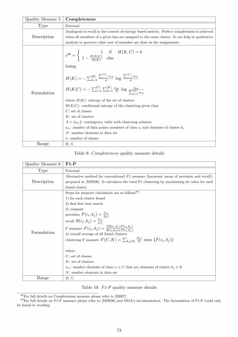
Quality Measure 5 CompletenessType External

DescriptionAnalogous to recall in the context of entropy based metrics. Perfect completeness is achievedwhen all members of a given lass are assigned to the same cluster. It can help in qualitativeanalysis to perceive what sort of mistakes are done in the assignments.

Formulation

c68 =

1 if H(K,C) = 01− H(K|C)

H(K) else

being

H(K) = −∑|K|k=1

∑|C|c=1 ack

n log∑|C|

c=1 ack

n

H(K|C) = −∑|C|c=1

∑|K|k=1

ackN log ack∑|K|

k=1 ack

where H(K): entropy of the set of clustersH(K|C): conditional entropy of the clustering given classC: set of classesK: set of clustersA = aij: contingency table with clustering solutionaij : number of data points members of class ci and elements of cluster kj

N : number elements in data setn: number of classes

Range [0, 1]

Table 9: Completeness quality measure details

Quality Measure 6 F1-PType External

DescriptionAlternative method for conventional F1 measure (harmonic mean of precision and recall),proposed in [MSE06]. It calculates the total F1 clustering by maximizing its value for eachfound cluster.

Formulation

Steps for measure calculation are as follows69:1) for each cluster found2) find first best match3) computeprecision P (ci, kj) = nij

|kj |recall R(ci, kj) = nij

|ci|

F measure F (ci, kj) = 2R(ci,kj)P (ci,kj)R(ci,kj)+P (ci,kj)

4) overall average of all found clustersclustering F measure F (C,K) =

∑kj∈K

|kj |N max F (ci, kj)

whereC: set of classesK: set of clustersnij : number elements of class ci ∈ C that are elements of cluster kj ∈ KN : number elements in data set

Range [0, 1]

Table 10: F1-P quality measure details68For full details on Completeness measure please refer to [RH07].69For full details on F1-P measure please refer to [MSE06] and MOA’s documentation. The formulation of F1-P could only

be found in wording.

73

Quality Measure 7 F1-RType External

DescriptionAlternative method for conventional F1 measure (harmonic mean of precision and recall),proposed in [MSE06]. It calculates the total F1 clustering by maximizing its value for eachground-truth class.

Formulation

Steps for measure calculation are as follows70:1) for each cluster found2) find first best match3) computeprecision P (ci, kj) = nij

|kj |recall R(ci, kj) = nij

|ci|

F measure F (ci, kj) = 2R(ci,kj)P (ci,kj)R(ci,kj)+P (ci,kj)

4) overall average of each ground-truth classclustering F measure F (C,K) =

∑ci∈C

|ci|N max F (ci, kj)

whereC: set of classesK: set of clustersnij : number elements of class ci ∈ C that are elements of cluster kj ∈ KN : number elements in data set

Range [0, 1]

Table 11: F1-R quality measure details

Finally, we define the quality measure we will use to do benchmarking:

Quality Measure used Q AVG (AVG of Quality Metrics)Type Combination of Internal & External

Description Average of CMM, Rand Statistic, Silhouette Coefficient, Homogeneity, Completeness, F1-Pand F1-R.

Formulation

Q AV G = CMM+RI+SC+h+c+F1 P+F1 R7

whereCMM : CMM Cluster Mapping MeasureRI: Rand IndexSC: Silhouette Coefficienth: Homogeneityc: CompletenessF1 P : F1-PF1 R: F1-P

Range [0, 1]

Table 12: Q AV G quality measure details

70For full details on F1-R measure please refer to [MSE06] and MOA’s documentation. The formulation of F1-R could onlybe found in wording.

74

3.3 Quality tests - Synthetic data

Now that we have defined the quality measure to use (Q AV G = CMM+RI+SC+h+c+F1 P+F1 R7 ), we will

need synthetic data for testing. We use MOA’s capabilities to generate synthetic streaming data by usingRandom RBF Generators71. This gives us the flexibility to create very diverse scenarios and measure thequality results of the clustering delivered by Clustream, Denstream and Clustree in each. We should noticethat generated data is normalized within the [0,1] range.

We therefore design a comprehensive set of scenarios where numbers of clusters (few, medium amount,many), radius sizes (small, medium size, big), dimensionality (2, 5, 20, 50) and noise levels (10%, 33%) aresystematically combined. We produce 10 test type scenarios, combining all the elements above with thevalue ranges described in Table 13:

Number of clusters- few: 2 to 5- medium amount: 5 to 11- many: 12 to 44

Cluster radius length

in d dimensions:- small: 0.001 to 0.05- medium size: from 0.05 to 0.2572

- big: 0.11 to 0.25 to

- Observation: MOA generates synthetic data in normalized space. StreamLeader isdesigned to work in that space too.

Dimensionality 2, 5, 20, 50

Noise levels 10%, 32.8%

Table 13: Elements to create synthetic test scenarios

We prepare 10 different scenarios. Type 1 to 5 combine multiple cluster sizes with different amount ofclusters, from low to high dimensionality, all in a 10% noise environment. Type 6 to 10 repeat the same sortof test scenarios but with noise levels increased to 33%. Each test in MOA will consist of 500000 streaminginstances. It also contains concept drift, including cluster speed in the d space (speed = 500, clusters movea predefined distance of 0.01 every 500 instances), event frequency (each 50000 instances), events are eithercluster creation, deletion, merging or split73 when event frequency completes. Some parameters were taken asdefault, namely decay horizon = 1000, (instance)decay threshold = 0.01, evaluation frequency = 1000.We used the given random seeds (modelRandomSeed = 1, instanceRandomSeed = 5).

With such tests, we aim to check how robust the algorithms are in terms of quality. We also want tocheck the sensibility in terms of parametrization. We opt to run each algorithm first with default then withoptimal parametrization. Below we describe what we understand by these two different setups:

- DEFAULT PARAMETRIZATION: Parametrization MOA74 gives by default to each algorithm. Val-ues are as follows:

- StreamLeader : horizon = 1000, d max = 0.11.As stated before, a default value of 0.11 allows expansion that covers a big portion of the normalized

d-dimensional space but also the contraction to discover small cluster.

- Clustream: horizon = 1000, maxNumKernels = 100, kernelRadiFactor = 2.As we will see in optimal parametrization, this provides a good micro-ratio for up to 9 or 10 clusters.

- Clustree: horizon = 1000, maxHeight = 8.71Please refer to Streaming Terminology section for further details.72Medium size is generated creating clusters with radius ranging from 0.001 to 0.25.73In some configurations, MOA crashed when splitting or creating new clusters, so we had to deactivate those options for

those tests.74MOA Release 2014.11

75

This height value for the tree is in line with what the authors mention in their published paper in[KABS11], where they use heights ranging from 7 to 11.

- Denstream (with DBSCAN): horizon = 1000, epsilon = 0.02, beta = 0.2, mu = 1, initPoints = 1000,offline = 2, lambda = 0.25, processingSpeed = 100

We already see the heavy and complex parametrization the algorithm needs. In general, these need tobe fine-tuned according to the data we are receiving. Parameters guide the algorithm in how data should begathered within common areas of density or noise elimination, and they are used first by Denstream in theonline phase and then by DBSCAN in the offline. Authors describe in [CEQZ06] that parameters shouldadopt the following setting: ε (neighbourhood) = 16 β (outlier threshold) = 0.2 µ (weight threshold formicro-cluster to exists as such) = 10 InitPoints = 1000 λ (decay factor) = 0.25 processingSpeed = 1000

We note that MOA’s parametrization is different. So we use MOA’s as we did with the other algorithms.We still can try to adjust the parameters when we do optimal parametrization.

- OPTIMAL PARAMETRIZATION as specified by corresponding published paper or adjusting theparameters as good as possible to the knowledge we have of the incoming stream (we know ground-truthbecause we specify the generating data distributions):

- StreamLeader : We adjust radius d max to a size around 15% smaller than the radius of the biggeststructure we will receive in the stream. Doing that, expansion capabilities will be used to cover the biggestcluster entirely. If at the same time several much smaller clusters do appear, we want that d max as smallas possible in order capture them individually and not together with bigger clusters that can cover several.

- Clustream: As described in [AHWY03], in order to achieve quality clustering the algorithm needs thatthe number of micro-clusters is larger than the one for natural clusters. That that can be inefficient tomaintain if the number increases enough. Therefore a micro-ratio is defined as number micro−clusters

number natural clusters with avalue of at least 10 or above to provide quality results with enough low granularity. KernelRadiFactor = 2 isthe optimal value to calculate CFs radius, trade-off between detecting new clusters without creating outliers.

- Clustree: horizon = 1000, maxHeight = 14.We give the tree much larger capacity as compared to default parametrization. According to the au-

thors in [KABS11], height of 7 to 11 were compared, with higher heights rendering lower granularitieswhich supposedly let the offline phase achieve higher quality clustering by using conventional stream clus-tering algorithms. Height = 14 increases substantially the detail in granularity as compared to defaultparametrization and also having in mind the values used in the original paper.

- Denstream (with DBSCAN):When trying to use the parametrization specified by the authors in [CEQZ06], we realize that the

value ranges are not allowed by MOA. We can therefore not replicate exactly its values. We have tried tofine-tune the parameters according to the paper and according to the test scenarios, but the ranges wereagain not accepted by MOA. A reason for this could be the normalized environment where MOA works,so we tried to scale-down all parameters accordingly but still, proportions could not be maintained for allparameters. Since Denstream is the only algorithm available that allows arbitrary-shaped clustering, wedecide to, at least, use a configuration that works, keeping in mind that it is most likely not an optimal one.We use neighborhood ε = 0.16 to define a bigger data neighborhood than what default parametrization uses.

Table 14 shows first the scenarios with 2d visual representation of what the tests would look like inMOA. Table 15 shows the quality results of each algorithm in each scenario. The table contains:

10 scenarios * 4 dimensions * 2 (default VS optimal) parametrization = 80 different configurations.Parametrization for each configuration is different, while respecting the scenario. Each configuration

requires execution of each algorithm to gather 7 measures. 80 configurations * 3 runs75 = 240 tests.Each test requires the corresponding parametrization for each algorithm and generates 7 quality metrics.Performing 10 runs per test would render 2400 test in total, which is unfeasible76, so we run them only once.

75Each configuration requires three runs, first StreamLeader VS Clustream, second StreamLeader VS Denstream, third Stream-Leader VS Clustree.

76We will perform 10 runs per tests when we proceed with scalability testing.

76

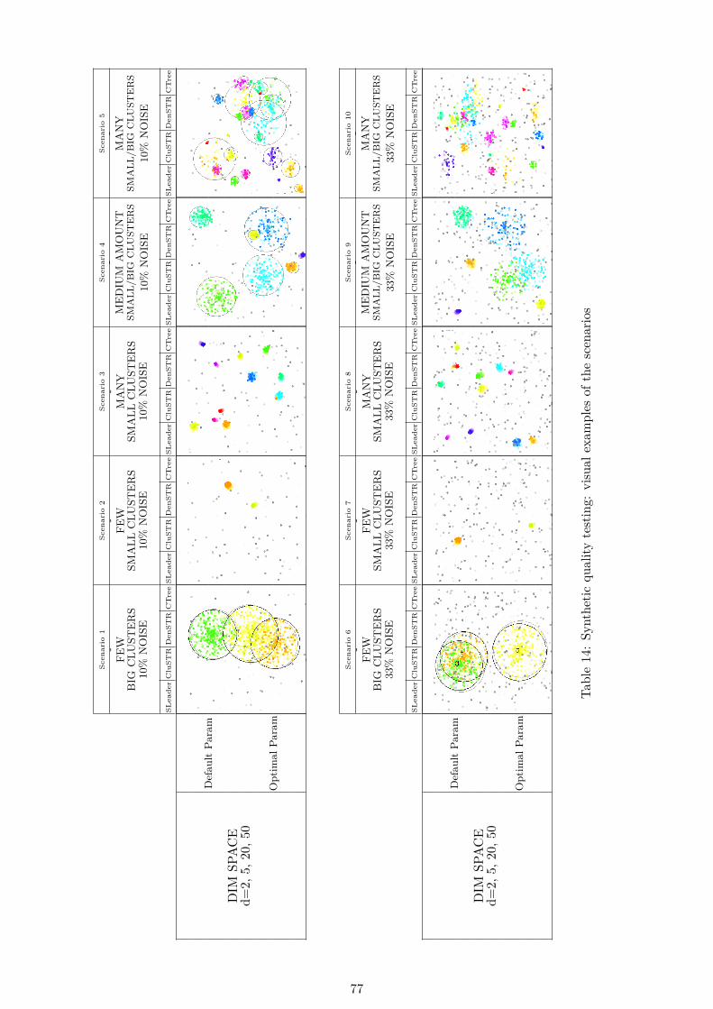
Scen

ario

1Sc

enar

io2

Scen

ario

3Sc

enar

io4

Scen

ario

5-

FEW

BIG

CLU

STE

RS

10%

NO

ISE

-FE

WSM

ALL

CLU

STE

RS

10%

NO

ISE

-M

AN

YSM

ALL

CLU

STE

RS

10%

NO

ISE

-M

ED

IUM

AM

OU

NT

SMA

LL/B

IGC

LUST

ER

S10

%N

OIS

E

-M

AN

YSM

ALL

/BIG

CLU

STE

RS

10%

NO

ISE

SLea

der

Clu

STR

Den

STR

CT

ree

SLea

der

Clu

STR

Den

STR

CT

ree

SLea

der

Clu

STR

Den

STR

CT

ree

SLea

der

Clu

STR

Den

STR

CT

ree

SLea

der

Clu

STR

Den

STR

CT

ree

DIM

SPA

CE

d=2,

5,20

,50

Def

ault

Para

m

Opt

imal

Para

m

Scen

ario

6Sc

enar

io7

Scen

ario

8Sc

enar

io9

Scen

ario

10-

FEW

BIG

CLU

STE

RS

33%

NO

ISE

-FE

WSM

ALL

CLU

STE

RS

33%

NO

ISE

-M

AN

YSM

ALL

CLU

STE

RS

33%

NO

ISE

-M

ED

IUM

AM

OU

NT

SMA

LL/B

IGC

LUST

ER

S33

%N

OIS

E

-M

AN

YSM

ALL

/BIG

CLU

STE

RS

33%

NO

ISE

SLea

der

Clu

STR

Den

STR

CT

ree

SLea

der

Clu

STR

Den

STR

CT

ree

SLea

der

Clu

STR

Den

STR

CT

ree

SLea

der

Clu

STR

Den

STR

CT

ree

SLea

der

Clu

STR

Den

STR

CT

ree

DIM

SPA

CE

d=2,

5,20

,50

Def

ault

Para

m

Opt

imal

Para

m

Tabl

e14

:Sy

nthe

ticqu

ality

test

ing:

visu

alex

ampl

esof

the

scen

ario

s

77

Scen

ario

1Sc

enar

io2

Scen

ario

3Sc

enar

io4

Scen

ario

5Sc

enar

io1.

.5-

FEW

BIG

CLU

STE

RS

10%

NO

ISE

-FE

WSM

ALL

CLU

STE

RS

10%

NO

ISE

-M

AN

YSM

ALL

CLU

STE

RS

10%

NO

ISE

-M

ED

IUM

AM

OU

NT

SMA

LL/B

IGC

LUST

ER

S10

%N

OIS

E

-M

AN

YSM

ALL

/BIG

CLU

STE

RS

10%

NO

ISE

-AV

GA

LLSC

EN

AR

IOS

10%

NO

ISE

SLea

der

Clu

STR

Den

STR

CT

ree

SLea

der

Clu

STR

Den

STR

CT

ree

SLea

der

Clu

STR

Den

STR

CT

ree

SLea

der

Clu

STR

Den

STR

CT

ree

SLea

der

Clu

STR

Den

STR

CT

ree

SLea

der

Clu

STR

Den

STR

CT

ree

DIM

SPA

CE

d=2

Def

ault

Par

am0.

620.

650.

250.

650.

830.

770.

730.

750.

710.

790.

630.

770.

740.

710.

530.

740.

570.

670.

320.

670.

690.

720.

490.

71O

ptim

alP

aram

0.62

0.65

0.48

0.67

0.83

0.77

0.51

0.77

0.91

0.84

0.23

0.82

0.76

0.71

0.34

0.74

0.67

0.68

0.33

0.71

0.75

0.73

0.38

0.74

DIM

SPA

CE

d=5

Def

ault

Par

am0.

800.

830.

230.

800.

870.

810.

700.

810.

900.

840.

320.

850.

920.

830.

540.

830.

910.

860.

310.

840.

880.

830.

420.

83O

ptim

alP

aram

0.82

0.83

0.5

0.84

0.87

0.81

0.69

0.82

0.92

0.93

0.28

0.90

0.92

0.83

0.55

0.87

0.92

0.90

0.28

0.90

0.89

0.86

0.46

0.87

DIM

SPA

CE

d=20

Def

ault

Par

amN

AN

AN

AN

A0.

900.

740.

710.

800.

950.

690.

370.

570.

930.

810.

700.

850.

950.

640.

32cr

ash

0.93

0.72

0.52

0.68

Opt

imal

Par

amN

AN

AN

AN

A0.

910.

740.

720.

800.

960.

910.

370.

720.

930.

810.

720.

870.

950.

920.

350.

750.

940.

840.

540.

78D

IMSP

AC

Ed=

50D

efau

ltP

aram

NA

NA

NA

NA

0.91

0.55

0.66

0.63

0.95

0.24

0.32

cras

h0.

930.

550.

550.

770.

950.

420.

360.

690.

930.

440.

470.

64O

ptim

alP

aram

NA

NA

NA

NA

0.91

0.55

0.67

0.66

0.96

0.67

0.32

0.42

0.93

0.73

0.58

0.70

0.95

0.73

0.36

0.64

0.93

0.67

0.48

0.60

Scen

ario

6Sc

enar

io7

Scen

ario

8Sc

enar

io9

Scen

ario

10Sc

enar

io6.

.10

-FE

WB

IGC

LUST

ER

S33

%N

OIS

E

-FE

WSM

ALL

CLU

STE

RS

33%

NO

ISE

-M

AN

YSM

ALL

CLU

STE

RS

33%

NO

ISE

-M

ED

IUM

AM

OU

NT

SMA

LL/B

IGC

LUST

ER

S33

%N

OIS

E

-M

AN

YSM

ALL

/BIG

CLU

STE

RS

33%

NO

ISE

-AV

GA

LLSC

EN

AR

IOS

33%

NO

ISE

SLea

der

Clu

STR

Den

STR

CT

ree

SLea

der

Clu

STR

Den

STR

CT

ree

SLea

der

Clu

STR

Den

STR

CT

ree

SLea

der

Clu

STR

Den

STR

CT

ree

SLea

der

Clu

STR

Den

STR

CT

ree

SLea

der

Clu

STR

Den

STR

CT

ree

DIM

SPA

CE

d=2

Def

ault

Par

am0.

570.

570.

210.

570.

860.

590.

540.

600.

680.

640.

510.

640.

730.

610.

490.

620.

570.

590.

290.

600.

680.

600.

400.

60O

ptim

alP

aram

0.57

0.57

0.46

0.58

0.88

0.59

0.39

0.61

0.89

0.63

0.28

0.68

0.8

0.61

0.34

0.67

0.67

0.60

0.35

0.63

0.76

0.60

0.36

0.63

DIM

SPA

CE

d=5

Def

ault

Par

am0.

690.

590.

280.

610.

800.

700.

440.

690.

930.

800.

350.

850.

890.

810.

360.

840.

870.

740.

330.

820.

840.

730.

350.

76O

ptim

alP

aram

0.69

0.59

0.36

0.63

0.83

0.70

0.59

0.71

0.95

0.85

0.48

0.89

0.89

0.81

0.52

0.85

0.87

0.83

0.34

0.91

0.85

0.76

0.46

0.80

DIM

SPA

CE

d=20

Def

ault

Par

amN

AN

AN

AN

A0.

880.

510.

430.

780.

950.

340.

340.

850.

890.

510.

490.

770.

930.

330.

330.

800.

900.

420.

400.

80O

ptim

alP

aram

NA

NA

NA

NA

0.91

0.51

0.45

0.78

0.96

0.66

0.35

0.86

0.89

0.51

0.57

0.76

0.94

0.84

0.35

0.84

0.92

0.63

0.43

0.81

DIM

SPA

CE

d=50

Def

ault

Par

amN

AN

AN

AN

A0.

870.

470.

350.

590.

900.

120.

31cr

ash

0.92

0.39

0.38

cras

h0.

920.

120.

32cr

ash

0.90

0.27

0.34

0.52

Opt

imal

Par

amN

AN

AN

AN

A0.

900.

470.

400.

540.

940.

340.

320.

400.

920.

420.

370.

690.

930.

430.

320.

400.

920.

410.

350.

51

0.67

0.66

0.35

0.67

0.87

0.64

0.56

0.71

0.90

0.64

0.36

0.70

0.87

0.66

0.50

0.75

0.85

0.64

0.33

0.70

Tabl

e15

:Sy

nthe

ticqu

ality

test

ing:

resu

ltsfo

rea

chsc

enar

io

78

The table shows the throughout testing of each algorithm on each scenario. On the right side, we canalso see average results per algorithm for all scenarios and split per 10% and 30% noise respectively. Below,another summary per scenario type with no split by noise levels. On both summaries, the best result of thefour algorithms is underscored.

From each test, for each algorithm, we take the resulting 7 quality metrics mentioned before (CMM,Rand Statistic, Silhouette Coefficient, Homogeneity, Completeness, F1-P, F1-R) and calculate the final over-all quality as Q AV G = CMM+RI+SC+h+c+F1 P+F1 R

7 .

First thing we notice from the tests, is that Scenario 1 and Scenario 6 have NA77 results for dimen-sionality 20 and 50. The reason is that MOA can not create big (i.e radius 0.11 to 0.25) clusters with suchdimensionality, prompting to reduce radius in cluster creation and/or split. In general, working in medium(20) to high dimensionality(50), we had to reduce the cluster size in order to run the tests. Looking at thenumeric results, MOA’s visual representation of the clusters and evolution of the metrics as the test proceed,we can see multiple situations were the algorithms react interestingly. We can not display each situationand scenario graphically, so we draw some general conclusions looking at the numbers, and also describinghow the algorithms handle the scenarios with some visual representations:

1) Denstream is the worst performer most of the times:as mentioned before, we could not emulate the author’s suggested parametrization in MOA for the optimalsetting, therefore we had to choose one that at least executed. MOA’s default setting was also different fromauthor’s, so we should look at Denstream’s results with caution.

2) Clustree crashed in five scenarios:this happened mostly in high dimensionality and with default parametrization. It is out of scope to inves-tigate the reasons of the crash so we will no comment on this further. In order to produce the statistics, avalue of 0.5 has been assigned to situations were the algorithm crashed. This value seems reasonable sincesometimes it could be a good result in a difficult scenario but sometimes could be low when other algorithmsave good performance.

3) All algorithms have problems with heavy cluster overlapping in very low dimensional spaces (2d):scenario 1 and 6 (FEW BIG CLUSTERS) seem to present challenging conditions for all four algorithms.This is because when we have big clusters changing position, the lower the dimensionality the higher thechances of overlapping and collisions. This has the effect that points will be found in the same location ind-dimensional space, therefore proximity metrics return a small distances and high similarity. The effectin StreamLeader, for instance, is that when two clusters get close enough, merging operations are triggered(Property 2 LeaderKernel additivity and merge operation), returning one cluster instead of the several thatmight exist as ground-truth. So when collisions do happen, StreamLeader tends to merge. All algorithmssuffer from the same effect, although they have an (unfair) important advantage because Clustream andClustree use k-means as offline conventional algorithm, receiving the true number of clusters from MOA, sothe chances to deliver better clustering in these situations are higher.We can see in Figure 37 a simplification of this effect caused by two clusters represented by two LeaderKernels(contour in red). The two clusters are identified in space in the upper side. In the middle, when they getclose enough, StreamLeader detects the instances and tries to encapsulate them all with a unique leader bycalculating the center of gravity according to DISTSL function. Lastly, when the clusters overlap totally, allalgorithms tend to represent the two ground-truth clusters with a unique one. We observe quality Metricsdropping down in general in such situations, specifically homogeneity, F1-P and F1-R which reflect theerrors properly. The way to properly parametrize StreamLeader in these situations, is with the assignmentof a smaller (than biggest cluster radius) D MAX. In this way, it tries to identify the masses first and thenexpand from inside out (expansion capabilities), as opposite to contract from outside down (contractioncapabilities).

77NA = Not Available.

79

Figure 37: Two LeaderKernels mapping true clusters (top) merge if true clusters get close enough (bottom)

4) Dimensionality higher than 2d:StreamLeader handles well situations with higher (greater than 2) dimensionality because of its design.Collisions are not so often, sparsity of the data is somehow expected, but inter-cluster distance is normallyhigher than inter-cluster distance among instances. StreamLeader captures the masses first, and can expandif necessary to a bigger cluster (default parametrization). With optimal D MAX it normally does not needto expand, and because collisions are not so frequent, it can contract and look for the most appropriateradius to capture the mass detected. Clustream, however, shows a noticeable decrease in quality resultswhen dimensionality increases. Clustree also, but not the same extend. The reason is caused by the useof cluster feature vectors CFs together with a conventional clustering algorithm. In high dimensions, CFsdo not have the capabilities to contract (like LeaderKernels do), therefore CFs tend to become bigger,occupying more space and distorting their centers. Since CFs are taken as pseudo-points and the centersare indeed distorted, then the clustering delivered is normally over-sized and returned clusters overlap withone another in space. Clustream can attenuate this negative effect when number of ground-truth clustersincreases by augmenting the micro-ratio to a factors bigger than 10. When this happens, it starts mappingpoints more closely, so the CFs tend to be of smaller radius. This has the effect of increasing the resultingclustering quality by taking more CFs, each representing a smaller and smaller set of points. But also twoconsiderable drawbacks: the performance gets degraded considerably (as we will see in scalability testing),and second such low level mapping produces some sort of overfitting, by mapping also the noise. In highnoise scenarios, quality drops substantially.We can se the effect of high dimensionality with default parametrization on the algorithms in Figure 38.Upper left plot shows true clusters (or ground-truth) in high d with 10% noise. Upper right shows theclustering provided by StreamLeader, where the LeaderKernels adjust remarkably well to the true clusters.Middle picture shows Clustream producing over-sized and overlapping micro-clusters (in green) and clus-tering (in blue). Bottom left shows Clustree with similar problems and bottom right Denstream, where itmaps almost exactly the points with many clusters.

80

Figure 38: micro-clusters (green) and clustering (blue) suffer distortions in high d in Clustream, Clustreeusing default parametrization

Same display with optimal parametrization in Figure 39:

Figure 39: micro-clusters (green) and clustering (blue) suffer distortions in high d in Clustream, Clustreeusing optimal parametrization

We observe that StreamLeader shows no difference in clustering delivered. This is because contractioncapabilities work well with default D MAX. Clustream, in this case behaves the same, because micro-ratiowas already above 10 with 7 clusters. In case we had a situation with 30 clusters, we would have observedthat optimal parametrization would have required around 300 CF ’s, and we would observe how each mappedclosely to each instance, producing the mentioned overfitting-like effect. Still it shows how big and smallCF ’s overlap in space, covering in many situations one another and delivering the offline phase a distortedview of the instances. Clustree shows how increasing height of tree from default 8 to 14, overfitting-like alsooccurs. Delivered clustering produces a really big cluster, covering most of the d normalized space, andoverlapping with other clusters. We recall that these representation in 2d does not imply overlapping ofclustering, but in this case, other views on other dimensions would show it. Also, the quality metrics reflectthis overlapping in clustering with a drop.

5) Noise:it poses a significant challenge for the algorithms except StreamLeader, which only experiments small de-

81

creases in quality. We can see in Figure 40, in the upper left side, seven clusters of different sizes in a streamwith 33% noise in high d.

Figure 40: micro-clusters (green) and clustering (blue) suffer distortions with heavy noise in Clustream,Clustree

In the upper right side, StreamLeader performs remarkably well, detecting the true clusters and buildingLeaderKernels describing them, using contraction capabilities. But the key in these scenarios is the noisetreatment it carries out in two phases, first percentile cuts and logarithmic cuts subsequently. The twotechniques combined seem to be very effective eliminating the heavy noise. In very heavy noise scenarioswe observed sometimes the effect of a LeaderKernel capturing noise and surviving the noise treatment, butit dissipated very quickly, distorting the quality measures only momentarily. Clustream and Clustree, inthe middle and bottom left corner respectively, have considerable problems because their CF ’s absorb thenoise as if they were points, overlapping heavily with one another. Furthermore, this distortion is passed onto the offline clustering algorithm producing over-sized (they include the noise) and overlapping clustering,causing drops in quality measures. Denstream in the bottom right side, seems to detect the very center ofmass of the cluster, although not covering the required space. MOA metrics still deliver bad quality results,so we will not comment further due to the problem with parametrization.

6) Optimal parametrization outperforms default parametrization:this is the case for all algorithms, but there are important differences. StreamLeader improves qualityonly marginally on each scenario. This is an indication that LeaderKernels expand and contract properly,adjusting their radius to the data and away from D MAX if needed. Only in one test type we can seesubstantial improvement, Scenario 3 & 8 with 2 dimensions and many small clusters, represented in Figure41. The reason is that those small clusters are found in very small space, so several can fall under theattraction of D MAX and therefore placed in the same LeaderKernel. Optimal setting means decreasingD MAX to a value similar of the size of radius of the true clusters. In this way, it does not capture severalclusters and concentrates only on the small mass represented by one single cluster. A mixture of small andbig clusters in very low d also challenges default parametrization. Still, this effect disappears when we moveinto 5, 20, 50 dimensions. We can see this effect in the picture below:

We already notice that optimal parametrization has no noticeable performance effects on StreamLeader,although this will be properly checked in scalability testing in next section.

82

Figure 41: StreamLeader delivering clustering (in red) with default & optimal parametrization in 2d space

With regards to Clustream, optimal parametrization depends on keeping micro-ratio above 10. Thishappens mostly in scenarios 3 & 5, with numerous clusters (20 or more). More micro-clusters are thereforeneeded (above 200 for a 20 cluster scenario, or above 300 with 30) which will then describe the streamwith a finer granularity, lowering substantially the radius of the CFs micro-clusters. This has the effect ofmapping also noise (and noticeable negative effects on performance, amplified when we move into higherdimensionality). Figure 42 shows the effects described above, with 24 true clusters as ground-truth in theplot in the upper side, micro-clusters (in green) and clustering (in blue) delivered by Clustream, with defaultparametrization on the left side and optimal on the right side.

Figure 42: Clustream clustering with default & optimal parametrization (micro-clusters green, clusteringred & blue)

We can observe that with default parametrization (100 micro-clusters), micro-ratio is below factor 10(100

24 = 4.16 ≤ 10) as recommended by the authors. Micro-clusters are therefore bigger and offline clusteringproduces heavily over-sized and overlapping clusters (bottom-left corner in the picture above), causingdegradation in clustering quality metrics. On the other hand, optimal parametrization implies manual

83

increase of number of micro-clusters to 260 to keep micro-ratio above 10 (26024 = 10.8 ≥ 10). This produces

the effect of decreasing micro-cluster’s size and also mapping data with lower granularity, which produces anoverfitting-like effect. This can be seen in the picture on the middle-right side, as very small micro-clustersgroup together and describe almost totally the cluster, together with bigger ones occupying big portions ofthe 20d space. Clustering produced is of higher quality than that of default parametrization, although highdimensionality causes the offline algorithm to still produce overlapping due to the micro-clusters. We shouldalso note that this effect would be amplified with high noise levels producing further drops in quality. Wealso experience substantial negative impact on runtime performance (further details on this effect on thescalability section).

Clustree suffers from same effects. Optimal parametrization of 14 levels of the tree provides finer granu-larity CFs than height 8 to summarize the data. It can increase the quality, but it is also very sensitive tonoise. In Figure 43, we can see same stream as shown in 42, 24 true clusters in the upper side, the effectsof both parametrizations for the Clustree, default in the left, optimal in the right, and comparison withclustering delivered by StreamLeader at the bottom, all in same scenario at same instant. StreamLeaderachieves higher accuracy, contracting in d space where the mass is and producing no overlapping. Clustreesuffers from overlapping and oversize clustering, regardless of parametrization used.

Figure 43: Clustree clustering with default & optimal parametrization. Also StreamLeader with optimal

7) Looking at quality results, StreamLeader outperforms, in average, Clustream, Denstream, Clustree:results based on dimensionality and on noise levels indicate that StreamLeader delivered better qualityclustering in average, both in default and optimal configurations. Only in dimensionality 2 with defaultparametrization, StreamLeader was outperformed by Clustream due to the high collision of clusters and theadvantage that Clustream has of using k-means with the real number of true clusters provided by MOA. Perscenario type, it outperforms in average again the contenders, only sharing the highest score with Clustreein scenario with few big clusters combining 10% & 33% noise levels.

8) Individual clustering quality metrics: default vs optimal parametrization:for each of the 216 tests78, we take the 7 quality metrics used. Figures 44, 45, 46 and 47 show how eachalgorithm performs on each metric in average, with default parametrization on the left side and optimal inthe right. We want to see: a) quality achieved and b) effect of parametrization on each metric:

78Experiments consisted of 240 tests except 16 that crashed in MOA, from scenario 1 & 6 (few big clusters with 10% & 33%noise levels) in dimensionality 20 & 50.

84

Figure 44: Synthetic results: average CMM and Silhouette Coef, default vs optimal parametrization

Figure 45: Synthetic results: average F1-P and F1-R, default vs optimal parametrization

85

Figure 46: Synthetic results: average Homogeneity and Completeness, default vs optimal parametrization

Figure 47: Synthetic results: average Rand Statistic and overall Q AV G, default vs optimal parametrization

86

With regards to parametrization, we can extract important information from the figures:

- with default parametrization, StreamLeader seems to outperform all other algorithms in each of themetrics with exception of Completeness. However, this was somehow anticipated because, as we mentionedbefore, techniques like Clustream filled the d space with over-sized CFs and overlapping clusters due to theuse of conventional clustering algorithms. When that is the case, Completeness renders very high qualityresult because all members of a single class are always assigned to the same cluster. But this also has avery negative collateral effect on homogeneity, which delivers quality when each cluster contains members ofa single class, which in this case hardly happens because big overlapping clusters contain much more thanjust one class. This is also noticeable in F1-R recall which drops in quality when clusters are over-sizedincluding instances of one class but also from other classes or just noise. F1-P shows higher values sincebigger clusters would retrieve most of the instances of a class. Last graph shows the average of all qualitymeasures, showing StreamLeader performing remarkably well and Clustree outperforming clearly Clustream

- with optimal parametrization, StreamLeader seems to outperform all other algorithms in each of themetrics again with exception of Completeness. The reasons are as above. We notice also that StreamLeaderonly improves marginally (default scored high already). This indicates that the contraction and expansioncapabilities of the LeaderKernels work well and capture the mass of the clusters effectively. Another takefrom the plots is that the other algorithms do improve substantially their quality, specially Clustream inF1-P, F1-R, homogeneity and Rand Statistic, which indicates that the micro-ratio needs to be adjustedproperly with the number of real clusters. Clustree improves also but to a lesser extend, still, showing a bet-ter overall performance than Clustream. Denstream showed poor performance, probably to the inadequateparametrization.

9) Average clustering quality metrics: 10% vs 33% noise levels:we do the same exercise averaging all metrics for all tests per noise level and produce the results shown inFigure 48 in the upper plots. For 10% noise environments in the left, StreamLeader seems to outperformthe other algorithms, while Clustream and Clustree have a similar performance. Introducing 33% noiselevels, in the right, does not seem to impact substantially StreamLeader, which indicates that the algorithmhas high tolerance to noise thanks to the combination of percentile, logarithmic cuts and the avoidance ofconventional clustering algorithms. Clustree gets impacted but not as much as Clustream, which experiencesa substantial drop in quality. This seems to corroborate what we expected since offline phase takes as inputthe noise captured by micro-clusters, which produced degradation in clustering.

10) Average clustering quality metrics: low dimensionality (d = 2, 5) vs medium/high (d = 20, 50):lastly, we analyze the general performance focusing on dimensionality. In Figure 48 in the lower plots, we seethat, in low dimensional space (d = 2, 5), StreamLeader outperforms again Clustream and Clustree, beingthese two similar in performance. Denstream lags behind. When we move into medium/high dimensionality(d = 20, 50), in the bottom right, StreamLeader delivers even higher quality. Reason, among others, is thatno offline conventional clustering algorithm is used based on LeaderKernels, which would tend otherwise tocreate over-sized clusters. Also, collisions in high d are normally reduced, allowing StreamLeader to focusonly on detecting the concentrated mass using expansion/contraction capabilities. Effective noise treatmentalso contributes to eliminate undesired LeaderKernels that captured noise. On the other hand, Clustreeexperiences substantial degradation in performance, although not as much as Clustream, which is heavilyaffected by noise. One of the reasons for their lower performance is that they collect as many CFs as theycan maintain in order to capture fine-grain encapsulation of the data stream. In higher dimensional space,hyper-spherical micro-clusters tend to grow bigger and contain everything they find in d space, includingnoise. Passing these encapsulations to the offline phase where conventional algorithm takes them as input(which can be already distorted) might cause degradation in clustering, including over-sized and overlappingclustering. If they use optimal parametrization to maintain a larger number of CFs, then their radius isreduced, they summarize in a very low detail, producing what it looks as overfitting-like capturing theneverything, including noise with individual CFs

87

Figure 48: Synthetic results: average overall quality Q AV G per noise levels and dimensionality

11) Overall Average clustering quality metrics:Finally, we average all metrics for all synthetic tests (Q AV G = CMM+RI+SC+h+c+F1 P+F1 R

7 ) peralgorithm and produce the following the plot shown in Figure 49 which describes the overall performancewith synthetic data. StreamLeader outperforms in quality Clustream, Clustree and Denstream. Thisconfirms that LeaderKernels describe efficiently the synthetic data stream, time window managementhandles well their aging, noise treatment is effective eliminating disturbances in underlying data generationand the attempt of using no conventional clustering worked remarkably well:

Figure 49: Synthetic results: overall quality performance for all scenarios

88

3.4 Quality tests - Real Data

Synthetic data is very useful when it comes to designing scenarios with different configurations, coming nor-mally in the form of Gaussian distributed points around centers in Rd. Real data sets can behave differentlyto those artificially generated though. Thus, we need to find real data that evolves significantly. Review-ing the literature, we find two datasets that have been used in clustering tasks and later in stream clustering:

- Forest Cover Type (KDD)- Network Intrusion Detection (KDD-CUP’99)

MOA provides the capability to feed data files by using the class FileStream. By adding headers to thefile, which explain the content of the data, MOA converts all observations contained into a data stream thatcan be fed to the algorithms. An example for such headings is the following:

@RELATION Forest Cover Type MOA input@ATTRIBUTE Elevation NUMERIC@ATTRIBUTE Aspect NUMERIC......@ATTRIBUTE Cover Type desc Spruce Fir,Lodgepole Pine,Ponderosa Pine,Cottonwood Willow,Aspen,Douglas fir, Krummholz

@DATA0.366561630964665,0.157946610042229,0.0310230063453802,0.152063116587451,0.21612095140829,0.0553723245473644, ... ,Aspen...

3.4.1 Data Set 1: Forest Cover Type

Forest Data Cover data set has been used frequently in the stream clustering literature, in StreamKM++[AMR+12] or Clustree [KABS11] among others. We will use it then in MOA to compare the algorithms.Table 16 contains a brief description of the dataset:

Real Data Set Name Forest Cover Type (KDD)Size 580K observationsGoal Cluster the 7 different types of forest trees found in the terrain

Description

The forest cover type for 30 x 30 meter cells obtained from US Forest Service (USFS)Region 2 Resource Information System (RIS) data. It contains 10 continuous variables:(Elevation, Aspect, Slope, Horizontal Distance To Hydrology, Verti-cal Distance To Hydrology Horizontal Distance To Roadways, Hillshade 9am , Hill-shade Noon , Hillshade 3pm , Horizontal Distance To Fire Points)

7 classes to cluster (forest cover types), in variable Cover Type desc:- Spruce/Fir- Lodgepole Pine- Ponderosa Pine- Cottonwood/Willow- Aspen- Douglas-fir- Krummholz

Min classes79 2Max classes80 7Avg classes81 4.02

Location http://kdd.ics.uci.edu/databases/covertype/covertype.html

Table 16: Forest Covert Type data set details79Minimum number of different classes appearing simultaneously.

89

We select settings for the data stream (default values decayHorizon = 1000, decayThreshold = 0.01 ,evaluationFrequency = 1000) and normalize the data. Then execute the streaming of the data and noticeagain is that visualization in streaming scenarios is an important field to be improved upon. Thankfully,MOA provides some basic visualization in 2d modes, which is helpful, but surely techniques like parallel barsin streaming version would be very useful for this sort of investigation. We even considered developing atechnique for this, but we realized that it would be far too ambitions for the scope of this work. We finallyselect some sets of informative dimensions and see that the classes are intertwined and broken in differentpieces, which poses certainly a real challenge to the algorithms. Figure 50 shows four different 2-dimensionalscreen-shots in MOA of the execution of the streaming of the data set, at one specific instant. This givesan idea of what the data looks like. Upper left picture displays the attributes Elevation vs Aspect. Upperright Elevation vs Horizontal distance to hydrology. Bottom left Elevation vs Vertical distance to hydrologyand finally bottom right Elevation vs Horizontal distance to roadways. We also identify four classes (fourtypes of forest cover) present in the stream at that instant (class 1...class 4). On the right plots, We observehow class 1, class 2 and class 3 appear in the visualization in different places. That already indicates thatcreating unique non-overlapping clusters for each class will be difficult.

Figure 50: Forest Cover Type: visualizing the stream using four different sets of attributes

We also realize that the calculation of the ground-truth or true clustering done by MOA will not bestraightforward as seen in Figure 51. MOA does this probably on-the-fly by capturing each class (allinstances belonging to the same label) with the smallest possible hyper-spherical cluster. We should bear inmind that this step is necessary in order to calculate external clustering measures. We observe seven oversizedand overlapping clusters (contour in black) covering each class label (forest cover type, i.e. Lodgepole Pine,Ponderosa Pine, etc). Quality measures could well be affected because of this.

Figure 51: Forest Cover Type: true clusters or ground-truth calculated on-the-fly by MOA

80Maximum number of different classes appearing simultaneously.81Average number of different classes appearing simultaneously.

90

Table 17 contains the parametrization chosen for the algorithms (horizon = 1000 for all):

Algorithm StreamLeaderDefault Param D MAX = 0.11Optimal Param D MAX = 0.17

Algorithm Clustream

Default Param - MaxNumKernels = 100- kernelRadiFactor = 2

Optimal Param - MaxNumKernels82= 150- kernelRadiFactor=2

Algorithm ClustreeDefault Param maxHeight = 8Optimal Param maxHeight = 14

Algorithm Denstream83

Default Param

- epsilon = 0.02- beta = 0.2- mu = 1- initPoints = 1000- offline = 2- lambda = 0.25- processingSpeed = 100

Optimal Param

- epsilon = 0.16- beta = 0.2- mu = 1- initPoints = 1000- offline = 2- lambda = 0.25- processingSpeed = 100

Table 17: Forest Covert Type: parametrization used for StreamLeader, Clustream, Denstream and Clustree.

Figure 52 displays the clustering provided by StreamLeader (contour in red) and Clustream (contour inblue) for the instant shown in Figure 50. Attributes chosen for visualization are Elevation vs Horizontaldistance to hydrology. Clustream produces as many clusters (seven) as ground-truth shows, probably becauseit receives from MOA the true number of clusters to discover, so this help is not to be expected in a realscenario. Still, they do not seem very consistent with the data. StreamLeader delivers four in optimalparametrization.

Figure 52: Forest Cover Type: clustering by StreamLeader (red) and Clustream (blue)82While 100 micro-clusters achieves micro-ratio ≥ 10, we still opt to increase that ratio to achieve finer granularity.83We recall that we could not replicate the author’s preferred parametrization for Denstream in MOA.

91

Finally we gather quality metrics for both default and optimal parametrization in Figures 53 (CMM andSilhouette Coef ), 54 (F1-P and F1-R), 55 (Homogeneity and Completeness), 56 (Rand Stat and Q AVG):

Figure 53: Forest Cover Type: CMM and Silhouette Coef default vs optimal parametrization

Figure 54: Forest Cover Type: F1-P and F1-R on default vs optimal parametrization

92

Figure 55: Forest Cover Type: Homogeneity and Completeness on default vs optimal parametrization

Figure 56: Forest Cover Type: Rand Statistic and Q AV G on default vs optimal parametrization

93

Together with the overall performance with both parametrizations in Figure 57:

Figure 57: Forest Cover Type: overall quality performance

According to the quality metrics, it is a very difficult data set to cluster in streaming. Homogeneityrenders very low quality for all algorithms except StreamLeader, which still suffers from a quality droparound in the middle of the experiment but then recovers. Completeness on the other hand shows weakperformance for StreamLeader, values even drop out of the plot. In general, the classes in general seem tobe fragmented in different pieces in several locations, so the algorithms struggle to find them using hyper-spherical clusters. Another factor of uncertainty is the way MOA calculates ground-truth and compare itwith final clustering to generate external quality clustering measures. All in all, StreamLeader outperformsagain in average Clustream, Denstream and Clustree. Table 18 displays average quality values obtainedwith default and optimal parametrization. While Denstream crashed in MOA delivering metrics in defaultparametrization, it outperformed Clustream and Clustree using optimal parameters, which could not improvetheir own results in any of the two parametrizations.

Forest Cover Type-

FEWBIG CLUSTERS

SLeader CluSTR DenSTR CTree

DIM SPACEd=10

Default Param 0.26 0.27 crash 0.27Optimal Param 0.37 0.27 0.36 0.27

Table 18: Forest Cover Type: quality test results

94

3.4.2 Data Set 2: Network Intrusion

This data set was used for the Third International Knowledge Discovery and Data Mining Tools Compe-tition, held together with KDD-99 The Fifth International Conference on Knowledge Discovery and DataMining in 1999. It can be found frequently in stream clustering research, i.e. StreamKM++ [AMR+12],Clustream [AHWY03], Denstream [CEQZ06], D-Stream [CT07] and Clustree [KABS11] among others. Table19 contains a brief description of the dataset:

Real Data Set Name Network Intrusion (KDD-CUP’99)Size 4.8 million connections

Goal The intrusion detector learning task is to build a network intrusion detector capable of distin-guishing between bad connections, called intrusions or attacks, and good normal connections.

Description

Data contains computer connections, defined as a sequence of TCP packets starting andending at some well defined times, between which data flows to and from a source IPaddress to a target IP address under some well defined protocol. Each connection is labeledas either normal, or as an attack, with exactly one specific attack type. Each connectionrecord consists of about 100 bytes.

It contains 42 total attributes (34 of those continuous used for clustering):

duration, protocol type , service , flag , src bytes , dst bytes , land , wrong fragment ,urgent , hot , num failed logins , logged in , num compromised , root shell , su attempted ,num root , num file creations , num shells , num access files, is host login , is guest login ,count , srv count , serror rate , srv serror rate , rerror rate , srv rerror rate , same srv rate ,diff srv rate , srv diff host rate , dst host count , dst host srv count , dst host same srv rate, dst host diff srv rate , dst host same src port rate , dst host srv diff host rate ,dst host serror rate , dst host srv serror rate , dst host rerror rate , dst host srv rerror rate

Cluster by type of connection in attack types:normal or 24 attack types (i.e satan, smurf, spy, warezmaster, neptune, multihop ,loadmodule , ipsweep , guess passwd, buffer overflow, etc)

Min classes84 1Max classes85 5Avg classes86 1.05

Location http://kdd.ics.uci.edu/databases/kddcup99/kddcup99.html

Table 19: Network Intrusion data set details

We choose settings for the data stream (default values decayHorizon = 1000, decayThreshold = 0.01 ,evaluationFrequency = 1000) and normalize the data. We have to do it manually because MOA turns outto normalize but values are not restricted to range [0,1] with this specific data set. We then visualize thestream in MOA to have a feeling of the data. We quickly see that this type of data is special in the waythat normal connections tend to be very similar in terms of duration, bytes transfered and so on. They aretherefore placed in the same position or very close in the normalized d space, almost in min or maximumvalues of the normalized variable. The reason is that attacks, on the other hand, present sudden substantialvariations in the variables (like rash increases in duration of connection, access files, root shell, etc), whichtake variables to the maximum or minimum values. Attacks also tend to be concentrated in a very short timespan, which in a streaming scenario appears as a flash in the middle of normal connections. The algorithmsare then confronted with very large periods of stability (normal connections) and sudden attacks lastinga fraction of that. An example of that would be, for instance, 40000 normal connections, combined withmoments where 50 or 200 abnormal (attacks) take place. We confirm this with the information describingthe data set in the table above, where Min classes = 1, Max classes = 5 (attacks), Avg classes = 1.05.

84Minimum number of different classes appearing simultaneously.85Maximum number of different classes appearing simultaneously.86Average number of different classes appearing simultaneously.

95

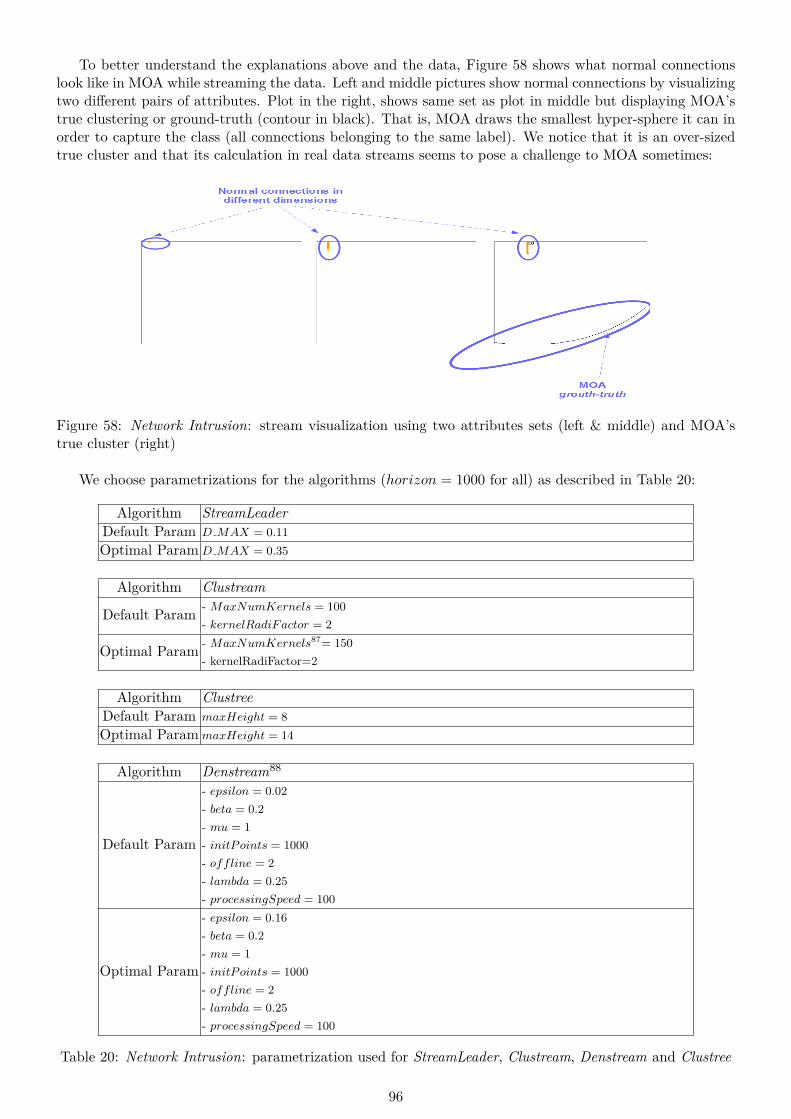
To better understand the explanations above and the data, Figure 58 shows what normal connectionslook like in MOA while streaming the data. Left and middle pictures show normal connections by visualizingtwo different pairs of attributes. Plot in the right, shows same set as plot in middle but displaying MOA’strue clustering or ground-truth (contour in black). That is, MOA draws the smallest hyper-sphere it can inorder to capture the class (all connections belonging to the same label). We notice that it is an over-sizedtrue cluster and that its calculation in real data streams seems to pose a challenge to MOA sometimes:

Figure 58: Network Intrusion: stream visualization using two attributes sets (left & middle) and MOA’strue cluster (right)

We choose parametrizations for the algorithms (horizon = 1000 for all) as described in Table 20:

Algorithm StreamLeaderDefault Param D MAX = 0.11Optimal Param D MAX = 0.35

Algorithm Clustream

Default Param - MaxNumKernels = 100- kernelRadiFactor = 2

Optimal Param - MaxNumKernels87= 150- kernelRadiFactor=2

Algorithm ClustreeDefault Param maxHeight = 8Optimal Param maxHeight = 14

Algorithm Denstream88

Default Param

- epsilon = 0.02- beta = 0.2- mu = 1- initPoints = 1000- offline = 2- lambda = 0.25- processingSpeed = 100

Optimal Param

- epsilon = 0.16- beta = 0.2- mu = 1- initPoints = 1000- offline = 2- lambda = 0.25- processingSpeed = 100

Table 20: Network Intrusion: parametrization used for StreamLeader, Clustream, Denstream and Clustree

96

We can see an examples of StreamLeader (left side, contour in red) and Clustream (right side, contourin blue) delivering clustering at specific moments in Figure 59, together with true clustering from MOA(contour in black). Upper plots show instant 1 in the stream, where StreamLeader seems to adjust well tothe set of points while Clustream delivers only a small clustering not covering all the connections. Bottomplots show another time instant 2, where StreamLeader creates a LeaderKernel that still seems to capturewell the connections, while Clustream delivers again a very small cluster.

Figure 59: Network Intrusion: clustering at two instants by StreamLeader (red) and Clustream (blue)

Figure 60 displays a very common situation that will explain why this time Denstream will deliver muchbetter quality results than what we saw in other sections of this work. Very similar connections imply verysimilar placing of the instances in d space, lasting also a considerable amount of time since normally thereare no cyber-attacks. Because there are no shapes to form, Denstream concentrates its clustering in verysmall areas, which almost map the instances themselves, achieving therefore higher scores. StreamLeader(red contour) creates a LeaderKernel capturing the connection, which is bigger than what seems necessaryin this set of attributes visualized. The LeaderKernel does not contract further even if it seems naturalto do so, probably because other dimensions show instances not concentrating so much89. Clustream andDenstream deliver a much smaller cluster.

Figure 60: Network Intrusion: clustering by StreamLeader (red), Clustream (blue) and Denstream (green)

87While 100 micro-clusters achieves micro-ratio ≥ 10, we still opt to increase that ratio to achieve finer granularity.88We recall that we could not replicate the author’s preferred parametrization for Denstream in MOA.89We found time consuming and difficult finding the right set of attributes to display. Advances techniques for visualizing

clustering in streaming scenarios is an evident need for the future.

97

Finally, Figure 61 shows a sudden and short-lived satan attack (in purple), which appears suddenly anddisappears very quickly. It contains two screen-shots with two time instants (instant 1 top plots whereattack just appears and instant 2 bottom plots, where the attack crossed the screen and banishes). Wecan see how StreamLeader (plots in the left, red contour) and Clustream (plots in the right, blue contour)react to the attack (fast change in data distribution). StreamLeader, at instant 1, covers initially the datawith one LeaderKernel and suddenly tries to adjust its size to the very fast moving sequence of connections,producing the effect we observe of co-center spheres. At instant 2, a big unique LeaderKernel captures thewhole tract of the attack. On the right side, Clustream also adjusts its micro-clusters as fast as it can atinstant 1. At instant 2 it produces two small clusters. We can also observe true clustering (black contour)in MOA, producing the bigger cluster of all. Due to the fast pace changes produced in this sort of attacks,we expect abrupt changes in the quality metrics.

Figure 61: Network Intrusion: Connection attack and reaction of StreamLeader (red) and Clustream (blue)

98

We gather all quality metrics for both default and optimal parametrization in Figures 62 CMM, 63 SilhCoef, 64 F1-P, 65 F1-R, 66 Homogeneity, 67 Completeness, 68 Rand Statistic, 69 Q AVG:

Figure 62: Network Intrusion: CMM on default vs optimal parametrization

Figure 63: Network Intrusion: Silhouette Coefficient on default vs optimal parametrization

99

Figure 64: Network Intrusion: F1-P on default vs optimal parametrization

Figure 65: Network Intrusion: F1-R on default vs optimal parametrization

100

Figure 66: Network Intrusion: Homogeneity on default vs optimal parametrization

Figure 67: Network Intrusion: Completeness on default vs optimal parametrization

101

Figure 68: Network Intrusion: Rand Statistic on default vs optimal parametrization

Figure 69: Network Intrusion: overall performance on default vs optimal parametrization

102

Together with the overall performance Q AV G with both parametrizations in Figure 70:

Figure 70: Network Intrusion: overall performance of StreamLeader, Clustream, Clustree and Denstream

As we see in the plots, the changes in metrics are very abrupt due to the nature of the attacks. Thefact that they are very short in duration produces the sudden drops in some of the metrics. Completenessin Figure 67 seems to be a very special case in experiencing the biggest decreases in quality. The reason isthat attacks occupy a place in the d space, away from normal connections, and StreamLeader can normallydetect them. The most difficult situation for the clustering task arises when the attacks come in the formof fast-moving instances in the d space. Then, LeaderKernels must track the moving target and adjustconstantly. In this cases, Completeness drops substantially because all members from the same class canalmost never be allocated to the same LeaderKernel which takes a certain amount of instances to reallocate(move) its leader. Looking at the values that MOA delivers for Completeness, we also observe extremelylarge negative values (i.e -8), even if the measure should be bounded within range [0,1]90. Another factorcould also be the way true clustering or ground-truth is calculated on-the-fly in MOA, because matchingagainst it is necessary for external measure calculation.

This problem immediately draws our attention to the fact that horizon is a key piece in this sort ofenvironment with streams having large periods of stability (normal connections) and sudden and abruptchanges (fast attacks). In normal situations, as we mentioned in former sections, a trade-off between stabil-ity/efficiency of the algorithms and rapid response is necessary. MOA allows horizon specification, but it isfixed, in this case for the 4.8 million stream instances. A technique like ADWIN or ADWIN2, as explained in[BG06] would be perfect for this data set to reduce horizon automatically, recalculate LeaderKernels fasterand and give a more accurate response to attacks.

Since 5.8 million instances overcrowd the plots, we also show separately the Q AV G overall metric foreach algorithm in Figure 71 and Figure 72. We observe how StreamLeader and Denstream suffer from intensedrops but achieve an overall higher quality than Clustream and Clustree.

90Analyzing the functioning of the measure in MOA is out of scope of this work.

103

Figure 71: Network Intrusion: overall performance of StreamLeader and Clustream

Figure 72: Network Intrusion: overall performance of Denstream and Clustree

104

To investigate further the drops in quality, we look with detail at metrics delivered StreamLeader only,shown in Figures 73, 74, 75 and 76. We want to trace where the sudden drops in quality originate. Wesee in Figure 75 that they are due to Completeness, which experiences decreases in quality reaching valuesof up to -8, even when the metric should be constrained to [0,1] in MOA. Such high negative values dragheavily the average quality for those instants.

Figure 73: Network Intrusion: CMM and Silhouette Coef for StreamLeader, default vs optimal parametriza-tion

Figure 74: Network Intrusion: F1-P and F1-R for StreamLeader, default vs optimal parametrization

105

Figure 75: Network Intrusion: Homogeneity and Completeness, default vs optimal parametrization

Figure 76: Network Intrusion: Rand Statistic and Q AV G for StreamLeader, default vs optimal parametriza-tion

106

Table 21 contains the numeric results of the tests. MOA crashes while producing Clustree’s measures.Ten values are set as NA (Not Available). If we were to assign default of 0.5 to those, Clustree woulddeviver average value of 0.65 and 0.65 for default and optimal parametrization respectively. StreamLeaderoutperforms again, in average, Clustream, Denstream and Clustree

Network Intrusion-

FEWSMALL CLUSTERS

SLeader CluSTR DenSTR CTree

DIM SPACEd=33

Default Param 0.71 0.79 0.80 crash

Optimal Param 0.90 0.79 0.82 crash

Table 21: Network Intrusion: quality test results

As side effect, we could use StreamLeader even as an attack warning system. In best case scenario, theconnections of an attack form a cluster (or clusters) that can be tracked in d space properly. If they reallocatetoo fast for our time window to track them efficiently, then we could theoretically detect those changes andadjust to a smaller horizon. Even if we could not adjust it, attacks trigger in StreamLeader the creation ofLeaderKernels to try capturing them. With proper D MAX, suddenly we detect attacks. Figure 77, upperplot displays number of classes in the data set as they appear in the stream (that is, classes = connectiontypes, so that several connection types implies a normal and several abnormal connections). Bottom plotcontains number of LeaderKernels maintained by StreamLeader at those specific moments. Above a certainthreshold, we get strong indications that connection attacks are taking place.

Figure 77: Network Intrusion: using StreamLeader as an attack warning system

107

3.5 Scalability and sensitivity tests

Regarding the aspect of theoretical complexity in stream clustering algorithms, we review the literature andfind that a comprehensive theoretical analysis on space and/or performance complexity seems not to bestandard in published papers. Clustream [AHWY03], Denstream [CEQZ06], Clustree [KABS11], D-Stream[CT07], StreamKM++ [AMR+12], among others, favor runtime performance and scalability testing instead.We therefore follow this approach and design scalability and sensitivity testing focusing on:

- number of clusters vs dimensionality, using default parametrization- number of clusters vs dimensionality, using optimal parametrization- number of clusters vs number of instances, using default parametrization

We use MOA command features to run the tests in console. Basic settings are: instanceLimit = 500000(stream size 500000 instances), measurecollectiontype = 0 (no measures collected), numClusterChange =0 (no change in number of clusters), KerneRadius = 0.025 (we keep clusters small so that we avoidcrashes in execution in high dimensional space91), RadiusChange = 0 (cluster radius does not change),Noise = 0.1 (10% noise), EventFreq = 50000 (one event every 50000 instances), MergeSplit = N andDeleteCreate = N (disabling events). We generate tests by changing numClus =? (number of clusters)and numAttr =? (dimensionality). An example of such command to test StreamLeader, D MAX = 0.04,RBF random generators to create the stream, 50 clusters of radius 0.025, disallow events creation/deletion,merging/splitting of clusters, (in normalized d space), 50 dimensions and half a million instances:

java -javaagent:sizeofag.jar moa.DoTask ”EvaluateClustering -l (StreamLeader.StreamLeader -d 0.04) -s (Random-RBFGeneratorEvents -K 50 -k 0 -R 0.025 -n -E 50000 -a 50) -i 500000”

We test each of the four algorithms against 2, 5, 20, 40 and 50 clusters, in spaces of dimensionality 2, 5,20 and 50. This results in 20 tests per algorithm, so 80 tests for all four algorithms. Each test in executed10 times to get average results, totaling 800 tests producing the average results in Figure 78:

Figure 78: Scalability: number of clusters VS dimensionality, (default parametrization)91In dimension d = 50, we had to reduce the cluster radius down to 0.02 because MOA needs small clusters if they are to be

created in such high dimensional space.

108

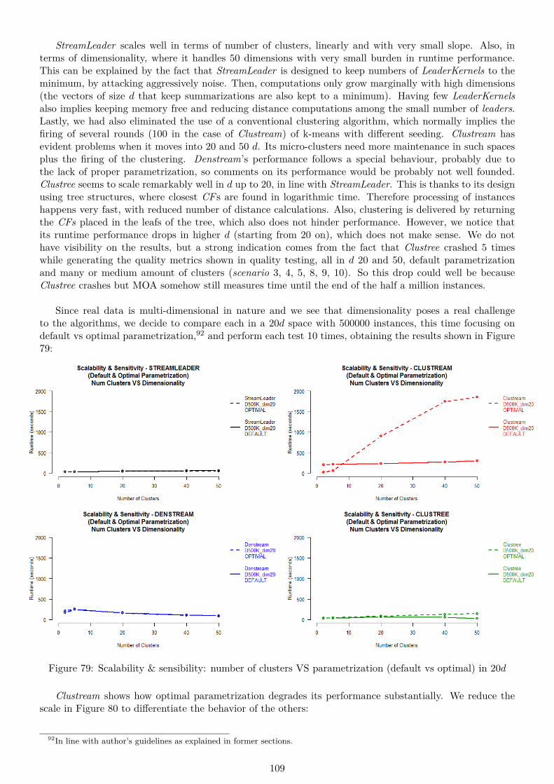
StreamLeader scales well in terms of number of clusters, linearly and with very small slope. Also, interms of dimensionality, where it handles 50 dimensions with very small burden in runtime performance.This can be explained by the fact that StreamLeader is designed to keep numbers of LeaderKernels to theminimum, by attacking aggressively noise. Then, computations only grow marginally with high dimensions(the vectors of size d that keep summarizations are also kept to a minimum). Having few LeaderKernelsalso implies keeping memory free and reducing distance computations among the small number of leaders.Lastly, we had also eliminated the use of a conventional clustering algorithm, which normally implies thefiring of several rounds (100 in the case of Clustream) of k-means with different seeding. Clustream hasevident problems when it moves into 20 and 50 d. Its micro-clusters need more maintenance in such spacesplus the firing of the clustering. Denstream’s performance follows a special behaviour, probably due tothe lack of proper parametrization, so comments on its performance would be probably not well founded.Clustree seems to scale remarkably well in d up to 20, in line with StreamLeader. This is thanks to its designusing tree structures, where closest CFs are found in logarithmic time. Therefore processing of instanceshappens very fast, with reduced number of distance calculations. Also, clustering is delivered by returningthe CFs placed in the leafs of the tree, which also does not hinder performance. However, we notice thatits runtime performance drops in higher d (starting from 20 on), which does not make sense. We do nothave visibility on the results, but a strong indication comes from the fact that Clustree crashed 5 timeswhile generating the quality metrics shown in quality testing, all in d 20 and 50, default parametrizationand many or medium amount of clusters (scenario 3, 4, 5, 8, 9, 10). So this drop could well be becauseClustree crashes but MOA somehow still measures time until the end of the half a million instances.

Since real data is multi-dimensional in nature and we see that dimensionality poses a real challengeto the algorithms, we decide to compare each in a 20d space with 500000 instances, this time focusing ondefault vs optimal parametrization,92 and perform each test 10 times, obtaining the results shown in Figure79:

Figure 79: Scalability & sensibility: number of clusters VS parametrization (default vs optimal) in 20d

Clustream shows how optimal parametrization degrades its performance substantially. We reduce thescale in Figure 80 to differentiate the behavior of the others:

92In line with author’s guidelines as explained in former sections.

109

Figure 80: Scalability & sensibility: number of clusters VS parametrization (default vs optimal) in 20d,reduced scale

And plot them together per type of parametrization in Figure 81:

Figure 81: Scalability & sensibility: number of clusters VS parametrization (default & optimal) in 20d,reduced scale (2)

We can draw some conclusions with the small size cluster setting. StreamLeader manages to even im-prove runtime performance when optimal parametrization is chosen. This can be explained by the fact thatadjusting the radius close to the size of the true biggest cluster causes fewer collisions, also occurring not sooften in higher d spaces so the StreamLeader spends most of its time contracting to the correct radius. Withdefault parametrization, probably D MAX is too large, therefore collisions with other LeaderKernels mightoccur, triggering then the merging operations, which implies computation over the always restricted set ofLeaderKernels. Still, it handles numerous clusters well using both parametrizations. Clustream pays a pricefor optimal tunning, having to maintain its micro-ratios with numerous micro-clusters in high d. Clustree

110

increases runtime performance with a higher slope than StreamLeader, avoiding this time the crashes itexperiences with default parametrization. Still, it outperforms Clustream clearly. This is again probablydue to the logarithmic access to the right CF when a new instance comes plus its internal handling of thetree and the fact of delivering clustering just by returning the CFs located in the leafs.

Lastly, we test again scalability by increasing number of instances in the data stream being launched atthe algorithms. We create data streams of different lengths (K=1000 instances) 100K, 250K, 500K, 1000K,2000K), in 20d space, using 5, 20 clusters and default parametrization. Rest of the configuration remainsthe same as in former synthetic tests, resulting in Figure 82:

Figure 82: Scalability: number of clusters VS number of instances, in 20d, default parametrization

StreamLeader scales again linearly with a small slope, increasing its runtime performance slightly whenthe stream contains 20 clusters. This means that no bottleneck occurs, and that the LeaderKernels absorbthe 2 million instances effectively (in less than 3 minutes). Clustree also handles the increasing streamefficiently, while Clustream seems to scale worse, taking around 12 minutes to process the data stream.

111

4 Part 4 - Conclusions and future work

4.1 Conclusions

In this thesis, we have developed a fast and accurate algorithm for clustering evolving streams of data,named StreamLeader, as it is based on the principles of the Leader clustering algorithm defined by JohnHartigan in [Har75].Our work needed to start with a review of the state of the art techniques in stream clustering. We cameto the conclusion that certain drawbacks are implicit to the design of most of the existing solutions. Theyuse a combination of online abstractions of the stream and offline phases, where resulting micro-clustersfrom online step are used offline as pseudo-points in a conventional clustering algorithm. First, the use ofconventional clustering in a streaming problem, does not seem entirely desirable. Second, micro-clusterstend to grow bigger in size in higher dimensional spaces, since data tends to be sparse, which implies thatfinal clustering also tends to be over-sized and overlapping. And third, noise can pose serious challenges tosuch approaches because it contaminates the micro-clusters and therefore the final clustering using them asbasis.These considerations gave us a clear idea of what we wanted to avoid and what to achieve with the Stream-Leader in a streaming scenario, while bearing in mind the characteristics we had to keep to follow leaderprinciples. Extending the concept of cluster feature vectors gave us an effective way to abstract parts ofthe stream and implement a functioning sliding window model, allowing LeaderKernels to age. We gavethem capability to contract and expand and made them very efficient in capturing groups of instances inthe multi-dimensional space based on a normalized proximity measure (distance) we developed. The use ofthese new units, called LeaderKernels proved very effective in encapsulating and capturing concept drift inthe stream. With them, we could absorb statistically the stream, but we needed to counter the tendency ofleader-based algorithms of filling the space with LeaderKernels. The solution to this problem gave us thekey for a more ambitions and integral solution, which avoids the need of a conventional clustering algorithmin the offline phase and that controls aggressively noise before it can contaminate resulting clustering. Wedesigned a novel approach to attack noise in the distribution of LeaderKernels, comprising of a combinedapplication of percentile and logarithmic cuts, aiming at noise located in the tail and in the elbow of thedistribution respectively.With regards to testing, we realized that it is common in the literature to use certain quality metrics whichare not optimal, due to either a tendency to deliver overoptimistic results (i.e purity) or because they lacknormalized results (i.e SSQ). Since individual metrics often focus on a partial view of the clustering quality,we deemed necessary to build a sound metric and did so by combining seven well-known clustering qualitymeasures, offering in this way a more comprehensive one. A framework to allow proper comparison ofstreaming solutions was also needed, so we put together 80 different use case configurations for synthetictesting, including noise levels, dimensionality and stream composition. Real data testing was also needed toput StreamLeader, Clustream, DenStrean and Clustree to the test. The results were encouraging, achievingand surpassing the initial expectations for the StreamLeader. Below the key milestones achieved:

1) We created StreamLeader, a new stream clustering algorithm based on the leader principles, and special-ized in detecting hyper-spherical clusters in multi-dimensional space.2) We integrated StreamLeader in MOA streaming platform.3) StreamLeader uses an alternative novel approach in order not to use any conventional clustering algorithmin the offline phase (which most of the other solutions do). It is based on percentile and logarithmic cuts onthe distribution of LeaderKernels, combined with contraction/expansion capabilities for cluster detection.4) To measure clustering quality, we avoided the use of single metrics (which is the most frequent case inthe literature) and created a sound metric which offers a more solid view of quality results.5) To test quality results, we designed a comprehensive set of 80 synthetic scenarios and also used real datato test the algorithms with multiple configurations and uniformly.6) StreamLeader outperformed, in terms of quality results, Clustream, Denstream and Clustree, in noisetolerance, dimensionality handling and stream composition.7) StreamLeader scaled remarkably well, in terms of cluster number, stream size, dimensionality andparametrization, outperforming in runtime performance Clustream, Denstrean and Clustree in most cases.8) StreamLeader achieves its performance with only one user-friendly parameter (Clustree 1, Clustreamrequires 2 and Denstream 7, in MOA).

112

4.2 Future work

As future work, there are plenty of areas where we could work to make StreamLeader more effective:

1) Even if completely 0% noise environment is not very likely, a new version will handle automatic ad-justments for the percentile cuts, which could be entirely disabled when necessary.

2) One important improvement would be to make the algorithm react faster to sudden changes in un-derlying data distributions. The need for this was clearly visible while testing Network Intrusion real dataset when short-lived attacks occurred suddenly, making it hard for the algorithms to adjust fast enoughand capture those instances in a cluster. This can be done via automatic horizon adjustment. An adaptivesliding window technique like ADWIN2 in [BG06] would be first candidate. If not in the algorithm itself,in MOA.

3) Another interesting area of improvement will be an automatic adjustment of the one parameter D MAX,so that, apart from contracting/expanding the cluster, it could also contract/expand the area of the influ-ence of the leader progressively in the multi-dimensional space. In this way, the algorithm would adjustitself automatically to concept drift, aiming at reaching an entirely autonomous stream clustering algorithm,needing no human intervention.

4) Expanding the use of StreamLeader to other domains would be also very important. A natural pathfor improvement would be heterogeneous data streams, where instances would be made up by numericaland categorical attributes. Here we could experiment with proximity measures, like Gower similarity coeffi-cient. If MOA was expanded, StreamLeader could also theoretically handle textual domains, like documentclustering, via calculation of similarity metrics like TF-IDF or other faster light-weight metrics. UsingStreamLeader in Genetics or DNA analysis would be a potential area of work, where metrics like Hammingdistances could cluster similar proteins, while probably requiring some sort of sketches to keep ordering ofgenes within the protein. Other options could be logical metrics like Jaccard, Sokal and so on.

5) A distributed version of StreamLeader would also be a natural development. We could integrate itinto SAMOA (Scalable Advanced Massive Online Analysis). SAMOA is a distributed streaming machinelearning framework that contains a programming abstraction for distributed machine learning algorithms.Because of its special design, number of LeaderKernels is always kept to a minimum and number of distancecomputations to leaders are therefore restricted. However, we should study whether substantial runtimeimprovement could be made or not with the use of distribution. We should bear in mind that the order inwhich the instances arrive does impact how LeaderKernels are created, but since leaders do evolve throughre-calculation of all instances that fall within, then the ordering is not so critical in our algorithm. Therefore,parallelization of the data stream would be an option to consider.

113

5 Part 5 - Appendix

5.1 Stream clustering terminology

The following are high-level general definitions used in this work, intended to be used as quick reference:

Attribute: a quantity describing an instance. An attribute has a domain defined by the attribute type,which denotes the values that can be taken by an attribute.

Attribute (or variable-based) clustering: stream clustering model with the goal of finding attributesthat behave similarly though time.

Batch mode: Batch machine learning techniques are used when one has access to the entire trainingdata set at once.

Categorical: A finite number of discrete values. The type nominal denotes that there is no orderingbetween the values, such as last names and colors. The type ordinal denotes that there is an ordering, suchas in an attribute taking on the values low, medium, or high.

Cluster feature vectors or CF : structure used for summarizing the data stream in the online phaseby using an n-dimensional vector of numerical features that capture statistics representing a cluster.

Clustering algorithm: algorithm with the task of grouping a set of objects in such a way that objects inthe same group (called a cluster) are more similar (in some sense or another) to each other than to those inother groups (clusters).

Concept drift: In streaming scenarios, change in underlying generation data distributions.

Coreset: small weighted set S of points, such that for any set of k-cluster centers, the weighted clus-tering cost of the coreset is an approximation for the clustering cost of the original set P with a smallerrelative error.

Cosine similarity measure: measure of similarity between two vectors of an inner product space thatmeasures the cosine of the angle between them.

Damped window model (or time fading models): time window model where more recent instanceshave higher importance than older ones by assigning normally weights to the instances so that more recentinstances have higher weights than older ones, using for instance, decay functions.

Data set: A schema and a set of instances matching the schema.

Data stream: massive sequence of instances potentially unbounded.

Data stream mining: process of extracting knowledge structures from continuous, rapid data recordsforming a data stream.

Dimension: An attribute or several attributes that together describe a property. For example, a geo-graphical dimension might consist of three attributes: country, state, city.

Distance: subgroup of proximity measures, where normally a numerical description is provided to de-scribe how far apart objects are.

Euclidean distance: in Euclidean space, the distance between points x and y is the length ||x − y||2of the straight line connecting them (xy).

Feature vectors: an n-dimensional vector of numerical features that represent some object.

114

Grids: structures used for summarizing the data stream in the online phase by segmenting the d-dimensionalfeature space into equal parts and assigning density quantities to them.

Ground-truth (also true cluster): known cluster structure of a data set (or cluster labels).

Horizon: in a data stream, the set of instances to be considered whose weights are above a certain threshold.

Induction algorithm: An algorithm that takes as input specific instances and produces a model thatgeneralizes beyond these instances.

Instance: A single object of the world from which a model will be learned, or on which a model willbe used (e.g., for prediction). In most machine learning work, instances are described by feature vectors;some work uses more complex representations (e.g., containing relations between instances or between partsof instances).

Instance-based clustering: stream clustering model with the goal of finding instances that behave simi-larly though time.

Knowledge discovery: The non-trivial process of identifying valid, novel, potentially useful, and ulti-mately understandable patterns in data.

Landmark window model: time window model where portions of a data stream are separated by land-marks, which are relevant objects defined by, for example, time, or number of instances observed as velocityfactor, producing non-overlapping sections of the stream and where instances arriving after a landmark aresummarized until a new landmark appears.

LeaderKernel: extension of cluster feature vectors with expansion and contraction capabilities that allowto represent a potential true cluster in a streaming environment.

Machine learning: field of scientific study that concentrates on induction algorithms and on other al-gorithms that can be said to learn, and is one step in the knowledge discovery process.

Micro-cluster: see cluster feature vector.

Noise: recognized amounts of unexplained variation in a data sample.

Normalized space: space where unit vectors (spatial vectors of length 1) are chosen to form the basisof the space.

Object: see instance.

Object-based clustering: see Instance-based clustering.

Offline Phase: second phase of a stream clustering algorithm where final clustering is provided basedon the components provided in the online phase.

Online (or data abstraction phase): second phase of a stream clustering algorithm where stream-ing data is summarized at a high level using special data structures.

Outlier: observation falling outside the overall pattern of a distribution.

Overfitting: effect occurred when a statistical model describes random error or noise instead of the under-lying relationship.

Prototype arrays: Method used for abstracting the data stream in the online phase by summarizing

115

an array of representatives, where each one of them represents certain parts of the stream.

Proximity measure: metric that reflects the actual proximity between instances according to the fi-nal aim of the clustering, like distance, similarity or dissimilarity indexes.

Random RBF Generator: process that generates a random radial basis function stream. This generatorwas devised to offer an alternate concept type that is not necessarily as easy to capture with a decision treemodel. The RBF (Radial Basis Function) generator works as follows: A fixed number of random centroidsare generated. Each center has a random position, a single standard deviation, class label and weight. Newexamples are generated by selecting a center at random, taking weights into consideration so that centerswith higher weight are more likely to be chosen. A random direction is chosen to offset the attribute valuesfrom the central point. The length of the displacement is randomly drawn from a Gaussian distributionwith standard deviation determined by the chosen centroid. The chosen centroid also determines the classlabel of the example. This effectively creates a normally distributed hypersphere of examples surroundingeach central point with varying densities. Only numeric attributes are generated.

Similarity index: subgroup of proximity measures as real-valued function that quantifies the similar-ity between two objects, taken in some sense as the inverse of distance metrics.

Sliding window: time window model where assumption is taken that recent data is more relevant thanolder data by using FIFO queue concept.

Stream clustering algorithm: clustering algorithm designed to work with data streams.

Time window model: model designed for data stream scenarios to detect potential change in data distri-bution generation processes by analyzing only most recent data.

True clustering (or ground-truth): see ground-truth.

Supervised learning: techniques used to learn the relationship between independent attributes and adesignated dependent attribute (the label). Most induction algorithms fall into the supervised learningcategory.

Unsupervised learning: Learning techniques that group instances without a pre-specified dependentattribute. Clustering algorithms are usually unsupervised.

Weight (of an instance): in streaming scenarios using time window models, the numerical value assigned toan instance that decays as time elapses, normally represented as decay functions in damped window models.

Weight (of a LeaderKernel): The terms weight and mass are equal in this context and refer to the numberof instances allocated to a LeaderKernel.

Window model: see time window model.

116

5.2 References

References

[Agg07] Aggarwal, C. 2007. Data Streams - Models and Algorithms. Springer.

[Agg09] C. Aggarwal. A Framework for Clustering Massive-Domain Data Streams. In ICDEConference, 2009.

[AHWY03] Aggarwal, C. C., Han, J., Wang, J., and Yu, P. S. 2003. A framework for clustering evolvingdata streams. In Proceedings of the 29th Conference on Very Large Data Bases. 81-92.

[AHW+04] C. C. Aggarwal, J. Han, J. Wang, and P. S. Yu. A framework for projected clustering of highdimensional data streams. In VLDB, pages 852–863, 2004.

[ALY+10] C. Aggarwal, Y. Li, P. Yu, and R. Jin. On Dense Pattern Mining in Graph Streams, VLDBConference, 2010.

[AMR+12] Ackermann, M. R., Martens, M., Raupach, C., Swierkot, K., Lammersen, C., and Sohler, C.2012. Streamkm++: A clustering algorithm for data streams. ACM Journal of ExperimentalAlgorithmics 17, 1.

[AV06] D. Arthur and S. Vassilvitskii. K-means++: The advantages of careful seeding. In Bay AreaTheory Symposium, BATS 06, 2006.

[AV07] D. Arthur and S. Vassilvitskii. k-means++: the advantages of careful seeding. Proc. 18thACM-SIAM Sympos. Discrete Algorithms, pp. 1027-1035, 2007.

[AY06] C. Aggarwal, and P. Yu. A Framework for Clustering Massive Text and Categorical DataStreams. In SIAM Conference on Data Mining, 2006.

[AY10] C. Aggarwal, and P. Yu. On Clustering Graph Streams, SDM Conference, 2010.

[AZY11] C. Aggarwal, Y. Zhao, and P. Yu. Outlier Detection in Graph Streams, ICDE Conference,2011.

[B02] Barbara, D. 2002. Requirements for clustering data streams. SIGKDD Explorations (SpecialIssue on Online, Interactive, and Anytime Data Mining) 3, 23-27.

[BBD+02] B. Babcock, S. Babu, M. Datar, R. Motwani, and J. Widom. Models and issues in data streamsystems. In Proc. 21st ACM Symposium on Principles of Database Systems, 2002.

[BC00] Barbara D, Chen P (2000) Using the fractal dimension to cluster datasets, in Proceedings ofthe Sixth ACM-SIGKDD International Conference on Knowledge Discovery and Data Mining,pages 260–264. ACM Press.

[BF07] W. Barbakh and C. Fyfe. Inverse weighted clustering algorithm. Computing and InformationSystems, 11(2), 10–18, May 2007. ISSN 1352-9404.

[BF14] Bolanos M, Forrest J, Hahsler M (2014). “Clustering Large Datasets using Data StreamClustering Techniques.” In M Spiliopoulou, L Schmidt-Thieme, R Janning (eds.), DataAnalysis, machine learning and Knowledge Discovery, Studies in Classification, Data Analysis,and Knowledge Organization, pp. 135–143. Springer-Verlag.

[BG06] A. Bifet and R. Gavalda. Learning from time-changing data with adaptive windowing. 2006.Poster. In 2007 SIAM International Conference on Data Mining (SDM’07), Minneapolis,Minnesota.

[BG09] A. Bifet and R. Gavalda. Adaptive Parameter-free Learning from Evolving Data Streams.2009. IDA ’09 Proceedings of the 8th International Symposium on Intelligent Data Analysis:Advances in Intelligent Data Analysis VIII, pp. 249-260

117

[BHK+11] A. Bifet, G. Holmes, R. Kirkby, and B. Pfahringer. 2011. DATA STREAM MINING: APractical Approach. Tech. rep. University of Waikato. Retrieved fromhttp://heanet.dl.sourceforge.net/project/moa-datastream/documentation/StreamMining.pdf.

[BHP+10] Bifet A, Holmes G, Pfahringer B, et al. MoA: massive online analysis, a framework for streamclassification and clustering. Journal of machine learning Research. 2010;22:44–50.

[BK12] A. Bifet, R. Kirkby, Tutorial 1. Introduction to MOA Massive Online Analysis, March 2012.Retrieved from http://sourceforge.net/projects/moa-datastream/files/documentation/Tutorial1.pdf/download.

[BK+12] A. Bifet, R. Kirkby. Tutorial 2. Introduction to the API of MOA Online Analysis, March2012. Retrieved fromhttp://sourceforge.net/projects/moa-datastream/files/documentation/Tutorial2.pdf/download

[BSH+07] M. Brun, C. Sima, J. Hua, J. Lowey, B. Carroll, E. Suh, and E. R. Dougherty. Model-basedevaluation of clustering validation measures. Pattern Recognition, 40(3),807–824, 2007.

[CEQZ06] Cao, F., Ester, M., Qian, W., and Zhou, A. 2006. Density-based clustering over an evolvingdata stream with noise. In Proceedings of the Sixth SIAM International Conference onDataMining. SIAM, 328-339.

[CM05] G. Cormode and S. Muthukrishnan. An Improved Data-Stream Summary: The Count-minSketch and its Applications. In Journal of Algorithms, 55(1), 2005.

[CT06] T. Cover and J. Thomas. Elements of Information Theory (2nd Edition). Wiley-Interscience,2006.

[CT07] Chen, Y. and Tu, L. 2007. Density-based clustering for real-time stream data. In KDD ’07:Proceedings of the 13th ACM SIGKDD international conference on Knowledge discovery anddata mining. ACM Press, 133-142.

[DH01] Domingos, P. and Hulten, G. 2001. A general method for scaling up machine learningalgorithms and its application to clustering. In Proceedings of the 8th InternationalConference on machine learning. Morgan Kaufmann, 106-113.

[Don00] S. van Dongen. Performance criteria for graph clustering and markov cluster experiments.Technical Report INS-R0012, National Research Institute for Mathematics and ComputerScience in the Netherlands, Amsterdam, May 2000.

[Dunn74] J. Dunn. Well separated clusters and optimal fuzzy partitions. Journal of Cybernetics,4:95–104, 1974.

[EKS+96] Ester, M., Kriegel, H.-P., Sander, J., and Xu, X. 1996. A density-based algorithm fordiscovering clusters in large spatial databases with noise. In 2nd International Conference onKnowledge Discovery and Data Mining. 226-231.

[EKW12] A. Eldawy, R. Khandekar, and K. L.Wu. On clustering Streaming Graphs, ICDCSConference, 2012.

[ELL+10] B. Everitt, S.Landau, M. Leese, D. Stahl. Cluster Analysis, 5th Edition. Wiley, 2010.

[FC83] E. Folkes and C. Mallows. A method for comparingtwo hierarchical clusterings. Journal of theAmerican Statistical Association, 78:553–569, 1983.

[Fis87] Fisher, Douglas H. (1987). ”Knowledge acquisition via incremental conceptual clustering”.machine learning 2 (2), 139–172

[FTT03] G. Flake, R. Tarjan, and M. Tsioutsiouliklis, Graph Clustering and Minimum Cut Trees,Internet Mathematics (2003), 1(4), pp. 385–408.

[Gam07] Gama, J. 2010. Knowledge Discovery from Data Streams. Chapman Hall/CRC.

118

[GG07] Gama, J. and Gaber, M. M. 2007. Learning from Data Streams: Processing Techniques inSensor Networks. Springer.

[GK54] L.A. Goodman and W.H. Kruskal. Measures of association for cross classification. Journal ofthe American Statistical Association, 49:732–764, 1954.

[GMMO00] Guha, S., Mishra, N., Motwani, R., and O’Callaghan, L. 2000. Clustering data streams. InIEEE Symposium on Foundations of Computer Science. IEEE Computer Society, 359-366.

[GRL11] Gama, J., Rodrigues, P. P., and Lopes, L. 2011. Clustering distributed sensor data streamsusing local processing and reduced communication. Intelligent Data Analysis 15, 1, 3-28.

[Har75] J. Hartigan. Clustering Algorithms, chapter 3: Quick Partition Algorithms. Wiley, 1975.

[HCL+07] Q. He, K. Chang, E.-P. Lim, and J. Zhang. Bursty feature representation for clustering textstreams. SDM Conference, 2007.

[HK01] J. Han and M. Kamber. Data Mining: Concepts and Techniques. Morgan Kaufmann, 2001.

[HXD+04] Z. He, X. Xu, S. Deng, and J. Huang. Clustering Categorical Data Streams, The ComputingResearch Repository, 2004.

[JZC06] Jain A, Zhang Z, Chang EY (2006) Adaptive non-linear clustering in data streams, CIKM, pp122–131

[KABS11] Kranen, P., Assent, I., Baldauf, C., and Seidl, T. 2011. The clustree: indexing micro-clustersfor anytime stream mining. Knowledge and Information Systems 29, 2, 249-272.

[KKJ+11] Kremer H, Kranen P, Jansen T, Seidl T, Bifet A, Holmes G, Pfahringer B (2011) An effectiveevaluation measure for clustering on evolving data streams. In: Proceedings of the17thACMSIGKDD international conference on knowledge discovery and data mining, pp868–876

[Kle02] J. Kleinberg, Bursty and hierarchical structure in streams, ACM KDD Conference, pp.91–101, 2002.

[KR87] Kaufman, L. and Rousseeuw, P.J. (1987), Clustering by means of Medoids, in Statistical DataAnalysis Based on the L 1–Norm and Related Methods, edited by Y. Dodge, North-Holland,405–416.

[KR90] Kaufman, L. and Rousseeuw, P. 1990. Finding Groups in Data An Introduction to ClusterAnalysis. Wiley Interscience.

[LL09] S. Luhr and M. Lazarescu (2009), ”Incremental clustering of dynamic data streams usingconnectivity based representative points,” Data and Knowledge Engineering, vol. 68, pp. 1-27.

[Maq67] MacQueen, J. B. 1967. Some Methods for Classication and Analysis of MultiVariateObservations. In 5th Berkeley Symposium on Mathematical Statistics and Probability, L. M.L. Cam and J. Neyman, Eds. Vol. 1. 281-297.

[Mei05] M. Meila. Comparing clusterings—an axiomatic view. InICML, pages 577–584, 2005.

[MM02] G. Manku, and R. Motwani. Approximate Frequency Counts over Data Streams, VLDBConference,2002.

[MSE06] G. Moise, J. Sander, and M. Ester, “P3C: A Robust Projected Clustering Algorithm,” Proc.Sixth IEEE Int’l Conf. Data Mining (ICDM), 2006.

[Ord03] C. Ordonez. Clustering Binary Data Streams with K-means. In Data Mining and KnowledgeDiscovery Workshop, 2003.

[PL07] Park, N. H. and Lee, W. S. 2007. Cell trees: An adaptive synopsis structure for clusteringmulti-dimensional on-line data streams. Data and Knowledge Engineering 63, 2, 528-549.

119

[Rand71] W.M. Rand. Objective criteria for the evaluation of clustering methods. Journal of theAmerican Statistical Association, 66:846–850, 1971.

[RGP06] Rodrigues, P., Gama, J., and Pedroso, J. 2006. ODAC: Hierarchical clustering of time seriesdata streams. In Proceedings of the Sixth SIAM International Conference on Data Mining.499-503.

[RH07] A. Rosenberg and J. Hirschberg. V-measure: A conditional entropy-based external clusterevaluation measure. Proceedings of the 2007 Joint Conference on Empirical Methods inNatural Language Processing and Computational Natural Language Learning(EMNLP-CoNLL), pages 410–420, 2007.

[Rij79] C.J.V. Rijsbergen. Information Retrieval (2nd Edition). Butterworths, London, 1979.

[RMJ07] M. Rattigan, M. Maier, and D. Jensen, Graph Clustering with Network Sructure Indices,ICML Conference Proceedings (2007), pp. 783–790.

[SKK00] Michael Steinbach, George Karypis, and Vipin Kumar. A comparison of document clusteringtechniques. In Workshop on Text Mining, KDD, 2000.

[Sha96] S. Sharma, Applied multivariate techniques. New York: Wiley, 1996.

[Str+13] F.Stahl. Tutorial 3. Introduction to MOA Clustering, October 2013. Retrieved fromhttp://sourceforge.net/projects/moa-datastream/files/documentation/Tutorial3.pdf/download

[XW08] R. Xu, D. Wunsch. Clustering. Wiley, 2008.

[ZK04] Y. Zhao and G. Karypis. Empirical and theoretical comparisons of selected criterion functionsfor document clustering. ML, 55(3),311–331, 2004.

[ZRL97] Zhang, T., R. Ramakrishnon, y M. Livny. 1996. BIRCH: An efficient data clustering methodfor very large databases. Proceedings of the ACM SIGMOD Conference on Management ofData. Montreal (Canada): ACM.

[ZS02] Zhu, Y. and Shasha, D. 2002. StatStream: statistical monitoring of thousands of data streamsin real time. In Proceedings of the 28th International Conference on Very Large Data Bases.VLDB Endowment, 358-369.

120