trajectories of ﬂuid particles in a periodic water...

Phil. Trans. R. Soc. A (2012) 370, 1661–1676doi:10.1098/rsta.2011.0447

Trajectories of fluid particles in a periodicwater wave

BY HISASHI OKAMOTO1,* AND MAYUMI SHOJI2

1Research Institute for Mathematical Sciences, Kyoto University,Kyoto 606-8502, Japan

2Department of Mathematical and Physical Sciences, Japan Women’sUniversity, 2-8-1 Mejirodai Bunkyo-ku, Tokyo 112-8681, Japan

We compute trajectories of fluid particles in a water wave that propagates with a constantshape at a constant speed. The Stokes drift, which asserts that fluid particles are pushedforward by a wave, is proved using a new method. Numerical examples with variousgravity and surface tension coefficients are presented.

Keywords: partial differential equations; nonlinear analysis; water wave

1. Introduction

We consider two-dimensional progressive water waves that propagate with aconstant shape at a constant speed. Fluid motion is assumed to be irrotational.We are interested in the study of trajectories of fluid particles in the stationarycoordinate system. Trajectories in a coordinate system attached to the waveare easily computed by drawing contours (level curves) of the stream function.Examples are abundant [1]. On the other hand, we need to take some care tocompute trajectories in the stationary coordinate system. Longuett-Higgins [2]gives some examples for gravity waves, but we do not know examples of capillary–gravity waves. The first objective of this paper is to give some new examples. Wedraw trajectories of gravity, capillary–gravity and pure capillary waves.

It is well known (see Lamb [3] or Milne-Thomson [4]) that fluid particles inlinearized water waves of small amplitude move on a circle or an ellipse, dependingon whether the depth of water is infinite or finite, respectively. Therefore, the fluidparticle does not move on average, whereas the wave itself propagates with a non-zero speed. This is, however, a proposition that is valid only approximately. Infact, Stokes [5] discovered that a particle trajectory is not closed.

Recently, Constantin [6] mathematically proved that none of the trajectoriesin the gravity waves are closed. It was also proved that trajectories in somelinearized water waves are not closed either. See Constantin and co-workers [7,8]for the case of finite and infinite depth, respectively. The second objective of thispaper is to prove non-closedness of trajectories by a method different from thatof Constantin and co-workers [6,7]. Our proof may be of some use because ofits simplicity.*Author for correspondence ([email protected]).

One contribution of 13 to a Theme Issue ‘Nonlinear water waves’.

This journal is © 2012 The Royal Society1661

on May 21, 2018http://rsta.royalsocietypublishing.org/Downloaded from

mailto:[email protected]

http://rsta.royalsocietypublishing.org/

1662 H. Okamoto and M. Shoji

This paper is organized as follows. In §2, we give an account of the backgroundof the present problem. Following this, we prepare some notations and amathematical framework in §3. In §4, we study Crapper’s pure capillary waves.Gravity and capillary–gravity waves are computed in §5. Constantin’s theorem isproved in §6. Finally, concluding remarks are presented in §7.

2. Background

For historical material on water waves, we recommend Craik [9]. Here, wesummarize what is necessary for this paper.

Fluid particles in linearized gravity waves of small amplitude move on a circleor an ellipse. This was first recognized by Green [10, p. 280]. Stokes [5] thenconsidered a higher order approximation. In the second-order approximation,he found a term that is proportional to the time variable, hence the particletrajectory does not close, but the fluid particle moves, on average, in the samedirection as the wave. This phenomenon is now called the Stokes drift. If thereader looks at the figures in Van Dyke [11, p. 110] carefully, then he/she willfind some trajectories which are not closed.

Longuett-Higgins [2] considered gravity waves of any amplitude and computedapproximately the trajectories of particles. The paper also presents somelaboratory experiments, which seem to agree with his theory.

From the viewpoint of modern mathematicians, the argument of Stokes is nota rigorous proof of non-closedness of particle trajectories. It is Constantin [6] whofirst presented a rigorous proof of the Stokes drift. His result has many variants[7,8,12–14], which we will comment on in the following sections of this paper.

Recently, the paper of Chen et al. [15] came to our attention. The authorsof this paper computed approximate solutions of fifth order and compared themwith their laboratory experiments. The agreement seems to be very good, see alsoUmeyama [16].

These studies are concerned with irrotational waves. Particles in rotationalwaves behave quite differently. In fact, all the trajectories in Gerstner’s wave(discovered by Gerstner [17], and later independently by Rankine [18]) are circles,no matter how large the wave amplitude may be, see earlier studies [3,4,19,20].

3. Preliminaries

In the following text, we restrict ourselves to particles in irrotational waves. Inthe moving frame, where the wave profile looks stationary, we take (x , y) as thecoordinates. We set z = x + iy and identify the complex plane with the (x , y)-plane. In the stationary coordinate system, we take (X , Y ). They are related byX = x + gt, Y = y, where g is the propagating speed of the wave profile. As wedo not lose generality by normalizing g = −1 and setting the wavelength as 2p,we do so henceforth. Accordingly, we have X + t + iY = x + iy. Hereafter, we usethe notation of Okamoto & Shoji [1]. The reason that we use g = −1 rather thang = 1 is that we required many formulae in Okamoto & Shoji [1], where g = −1was employed, and we prefer compatibility with Okamoto & Shoji [1] to that ofearlier studies [6–8,12,13,15,19,21,22]. These earlier studies employed g = 1.

Phil. Trans. R. Soc. A (2012)



Trajectories of fluid particles 1663

The fluid is assumed to be incompressible and inviscid. The motion of fluidis assumed to be irrotational. Throughout this paper, except in §6b, we consideronly progressive waves on water of infinite depth. Using the complex potentialf = U + iV , where U is the velocity potential and V is the stream function, wedefine z as

z = exp(−if ). (3.1)

Our normalization implies that U and V are so normalized that |U | ≤ p, −∞ <V ≤ 0. Accordingly, z runs in and on the unit disc of the complex plane, namely,|z| ≤ 1. We define z = x + iy, which is conformally in one-to-one correspondencewith z and f . For later use, we define r and s by z = reis. We now set

i logdfdz

= u = q + it, (3.2)

which is regarded as an analytic function of z. Here, u is defined by the equalityon the left-hand side. The equality on the right-hand side implies just that thereal and imaginary parts of u are denoted by q and t, respectively. u satisfiesthat u(0) = 0, which simply implies that the velocity tends to unity as z → 0, i.e.as y → −∞.

It is shown by Okamoto & Shoji [1] that two-dimensional progressive wavesare characterized by the following Levi-Civita equation:

e2t dt

ds− pe−t sin q + q

dds

(et dq

ds

)= 0 (0 ≤ s ≤ 2p). (3.3)

Note that q and t in (3.2) are regarded as a function of z defined in the unit discof the complex plane. q and t in (3.3) denote q(1, s) and t(1, s), respectively.As an analytic function is uniquely determined by its boundary values, q(r, s)and t(r, s) are uniquely determined once q(1, s) and t(1, s) are given. As t is animaginary part of the analytic function q + it, t can be written as the Hilberttransform of q. Accordingly, we have

t(s) = 12p

∫p

−p

q(s) cots − s

2ds,

where t(s) = t(1, s) and q(s) = q(1, s). p and q in (3.3) are given by

p = gL2pg2

and q = 2pTmg2L

.

Here, L is the wavelength, g is the propagation speed, g is the acceleration dueto gravity, T is the surface tension and m is the density of the fluid. As we havenormalized with g = −1 and L = 2p, p is simply the acceleration due to gravity.

The issue of existence of the solutions was discussed in earlier studies [1,23].

4. Crapper’s waves

Crapper [24] discovered that the pure capillary wave is an exact solution whengravity is neglected (p = 0) and the surface tension is the only force acting on the





fluid surface. It is given by

dfdz

=(

1 + Az

1 − Az

)2

(z ∈ C, |z| ≤ 1), (4.1)

where −1 < A < 1 is a real parameter that is related to q in the following way:

q = 1 + A2

1 − A2,

see Okamoto & Shoji [1]. As (3.1) gives us

dz

df= −iz, (4.2)

(4.1) implies that

dzdz

= iz

(1 − Az

1 + Az

)2

= i(

1z

− 4A(1 + Az)2

). (4.3)

Integrating this, we obtain

z = i(

log z + 41 + Az

− 4)

. (4.4)

Here, the integral constant is chosen so that the free surface of the trivial solution(the one with A = 0) becomes the line segment y = 0, −p ≤ x < p. The free surfacein the moving frame is obtained if we set z = eis in (4.4). If 0 < r < 1 is fixed and sruns in 0 ≤ s < 2p, then a particle trajectory below the free surface in the movingframe is obtained. We draw in figure 1 some wave profiles (r = |z| = 1) and particletrajectories in the water (0 < r < 1). If |A| > 0.45467 · · · , the wave profile has self-intersection points, and it is an unphysical solution. We must therefore considerthose solutions only with |A| < 0.45467 · · · , see Okamoto & Shoji [1].

Once the trajectory z = z(t) in the moving frame is given, we can obtain thecorresponding z = z(t) by applying the inverse mapping of (4.4). But the concreteexpression of the inverse mapping does not seem to be available, and we proceedas follows. Using (4.3), we have

dzdt

= iz

(1 − Az

1 + Az

)2 dz

dt. (4.5)

On the other hand, we can obtain the complex velocity using (4.1). The velocityin complex number notation is (

1 + Az

1 − Az

)2

,

where the bar denotes the complex conjugate. This must be equal to dz/dt. Hence,(1 + Az

1 − Az

)2

= i(1 − Az)2

z(1 + Az)2

dz

dt.





A = 0.1

(a) (b)

(c) (d)

A = 0.25

A = 0.44 A = 0.47

Figure 1. Crapper’s waves in the moving coordinates: (a) A = 0.1, (b) A = 0.25, (c) A = 0.44 and(d) A = 0.47. r = 0.1, 0.2, 0.4, 0.6, 0.8, 1. The broken line shows the level y = 0. The arrows indicatethe directions of the particles. They move from left to right.

We therefore obtain

dz

dt= z|1 + Az|4

i|1 − Az|4 . (4.6)

If we represent z(t) in polar coordinates as z(t) = r(t)eis(t), then (4.6) becomes

ds

dt= −

(1 + 2Ar cos s + A2r2

1 − 2Ar cos s + A2r2

)2

anddr

dt= 0. (4.7)

We can solve this as

−t = −4b1 − b2

sin s

1 + b cos s+ 8b2

(1 − b2)3/2tan−1

⎛⎝

√1 − b1 + b

tan(s

2

)⎞⎠ + s

(−p < s < p), (4.8)

where b is defined by

b = 2Ar

1 + A2r2.





(As r is independent of t and is a constant for a given particle, we regard it asa parameter.) We have chosen the integral constant so that t = 0 corresponds tos = 0. Or, instead, we may choose s′ = p − s to have

t = 4b1 − b2

sin s′

1 − b cos s′ + 8b2

(1 − b2)3/2tan−1

⎛⎝

√1 + b1 − b

tan(

s′

2

)⎞⎠ + s′

(0 < s′ < 2p). (4.9)

Here, the integral constant is adjusted so that t = 0 at s′ = 0. When wederive (4.9), we should note an identity tan−1 x + tan−1(1/x) = p/2. It is easilyseen that we can choose a branch of tan−1, so that the right-hand side of (4.9)becomes smooth at s′ = p.

We are now ready to draw trajectories in the stationary frame. Using (4.4) andX + iY = x − t + iy, we have

X = 8b2

(1 − b2)3/2tan−1

⎛⎝

√1 − b1 + b

tan(s

2

)⎞⎠ − 1 + b2

1 − b2

2b sin s

1 + b cos s, (4.10)

Y = 2√

1 − b2

1 + b cos s− 2 + log r (4.11)

or

X = − 8b2

(1 − b2)3/2tan−1

⎛⎝

√1 + b1 − b

tan(

s′

2

)⎞⎠ − 1 + b2

1 − b2

2b sin s′

1 − b cos s′ , (4.12)

either will do, but we mostly use (4.12) and (4.11) in what follows.We now compute some trajectories. We suppose that one of the crests of the

wave starts from the y-axis at t = 0. We then consider the motion of severalparticles that lie on the y-axis at t = 0. We compute trajectories for 0 ≤ s′ ≤ 2p.This implies that we draw trajectories until the particle comes to the same heightas the initial position. Figure 2 shows the trajectories in the case of A = 0.44. Wesee that the particle on the free surface takes a long journey. Figure 3 shows sometrajectories when A = 0.25 and A = 0.1. No trajectory in these figures is closed,and the particles drift leftwards. As the wave is periodic, the trajectories actuallylook like figure 4.

When A = 0.44, we plot a trajectory in figure 5 that lies somewhat deep, r =0.02. It is not closed, but is very much like a circular curve. Note that decreasing rimplies increasing the depth and reducing the nonlinear effect. Therefore, figure 5complies with linear theory.

We now define the drift distance as

D(r) = X(s′ = 2p) − X(s′ = 0).

This is the distance between two consecutive crests in the stationary frame. Asis seen from (4.12), it can be expressed as

D(r) = − 8pb2

(1 − b2)3/2= −32pA2r2 1 + A2r2

(1 − A2r2)3. (4.13)





–3

–2

–1

0

1

2

3

4

–45 –40 –35 –30 –25X

Y

–20 –15 –10 –5 0 5

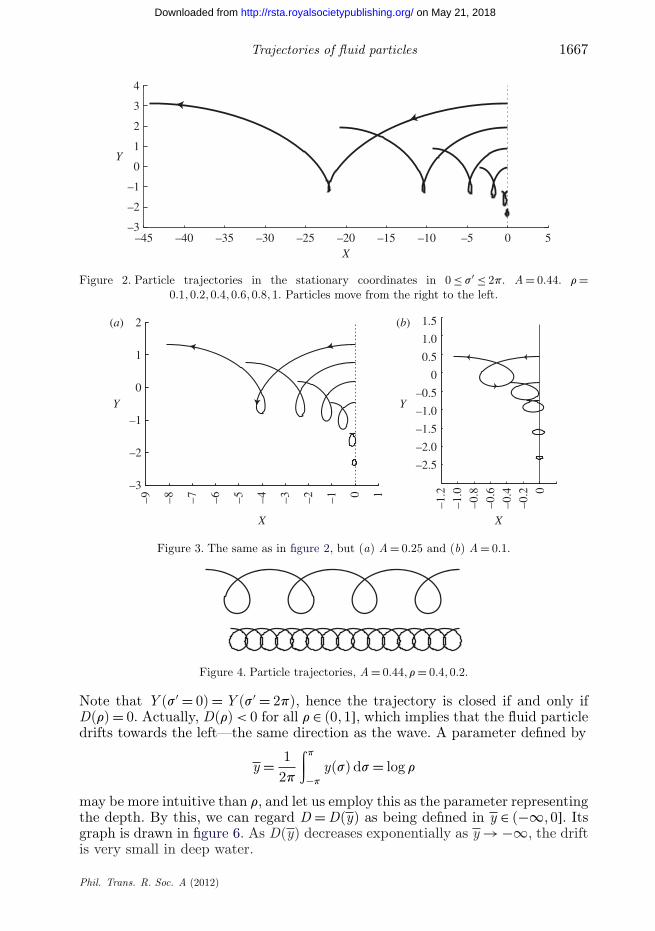
Figure 2. Particle trajectories in the stationary coordinates in 0 ≤ s′ ≤ 2p. A = 0.44. r =0.1, 0.2, 0.4, 0.6, 0.8, 1. Particles move from the right to the left.

–3

–2

–1

0

1

2

–9 –8 –7 –6 –5 –4 –3 –2 –1 0 1

–2.5

–2.0

–1.5

–1.0

–0.5

0

0.5

1.0

1.5(a) (b)

–1.2

–1.0

–0.8

–0.6

–0.4

–0.2 0

Y Y

X X

Figure 3. The same as in figure 2, but (a) A = 0.25 and (b) A = 0.1.

Figure 4. Particle trajectories, A = 0.44, r = 0.4, 0.2.

Note that Y (s′ = 0) = Y (s′ = 2p), hence the trajectory is closed if and only ifD(r) = 0. Actually, D(r) < 0 for all r ∈ (0, 1], which implies that the fluid particledrifts towards the left—the same direction as the wave. A parameter defined by

y = 12p

∫p

−p

y(s) ds = log r

may be more intuitive than r, and let us employ this as the parameter representingthe depth. By this, we can regard D = D(y) as being defined in y ∈ (−∞, 0]. Itsgraph is drawn in figure 6. As D(y) decreases exponentially as y → −∞, the driftis very small in deep water.





–3.95

–3.94

–3.93

–3.92

–3.91

–3.90

–3.89

–3.88

–3.87

–0.04 –0.03 –0.02 –0.01 0 0.01 0.02 0.03

Y

X

Figure 5. The particle trajectory in 0 ≤ s′ ≤ 2p. A = 0.44, r = 0.02.

–3.0

–2.5

–2.0

–1.5

–1.0

–0.5

0

–45 –40 –35 –30 –25 –20 –15 –10 –5 0

A = 0.44A = 0.25

A = 0.1

y

D ( y )

Figure 6. The drift distances for A = 0.1, 0.25, 0.44.

We next verify that the trajectories are almost circular in deep water. Weexpand (4.12) and (4.11) in small b to have

X = −2b sin s′ − 4b2s′ − b2 sin 2s′ + O(b3)

and Y = 2b cos s′ + 2b2 cos2 s′ + log r − b2 + O(b3).

}(4.14)

If we take only O(b) terms, we have a circle. The term −4b2s′ is responsible forthe Stokes drift.





–3.0

–2.5

–2.0

–1.5

–1.0

–0.5

0

0.5

1.0

1.5

–4.0

–3.5

–3.0

–2.5

–2.0

–1.5

–1.0

–0.5 0 0.5

(a) (b)

–4.0 –3.5

–3.0

–2.5

–2.0

–1.5

–1.0

–0.5 0 0.5

Y

X X

Figure 7. Particle trajectories in 0 ≤ t ≤ 2p. A = 0.25, r = 1, 0.8, 0.6, 0, 4, 0.2, 0.1 and (X |t=2p,Y |t=2p) with various r are plotted together. (a) The y-axis is mapped, at t = 2p, onto the greyline. (b) (X , Y ) with t = 2pk/10 (k = 1, 2, . . . , 10) with 0.05 ≤ r ≤ 1.

–4

–3

–2

–1

0

1

2

3

4

–6 –5 –4 –3 –2 –1 0 1–4

–3

–2

–1

0

1

2

3

4(a) (b)

–6 –5 –4 –3 –2 –1 0 1

Y

X X

Figure 8. (a,b) The same as in figure 7, but A = 0.44.

So far we have considered trajectories from one crest to the next crest. But thetime that elapsed during this motion is different from trajectory to trajectory.For instance, the particle on the free surface in figure 2 travels a long distanceand takes a lot of time. The travel time is considerably larger than 2p. On theother hand, the particle lying in deep water comes to the next crest in a timethat is close to 2p. Therefore, it would be interesting to consider trajectories fora fixed time interval, say, 0 ≤ t ≤ 2p. Figure 7a shows parts of trajectories for0 ≤ t ≤ 2p. Figure 7b shows positions of particles at t = 2pk/10 (k = 0, 1, . . . , 10),which started the y-axis at t = 0. Figure 8 shows the same data for a different A.

5. Gravity and capillary–gravity waves

We now study trajectories in the case of general (p, q). We consider onlysymmetric waves. Accordingly, q is assumed to be odd in s ∈ (−p, p). We start





with (3.3). By the Fourier spectral method, we obtain its approximate solution,

q(1, s) =N∑

n=1

an sin ns. (5.1)

For some solutions, N = 128 is enough, but some gravity waves requires a largeN such as N = 1024 [1]. With the coefficients an in hand, we compute

u(r, s) = q(r, s) + it(r, s) =N∑

n=1

anrn sin ns − iN∑

n=1

anrn cos ns

=N∑

n=1

(−i)an(reis)n = −i

N∑n=1

anzn

and

dfdz

= exp (−iu) = exp

(−

N∑n=1

anzn

).

As in the case of Crapper’s wave, we have

dz

dz= −iz exp

(−

N∑n=1

anzn

)or

dzdz

= iz

exp

(N∑

n=1

anzn

). (5.2)

The velocity is represented as

exp

(−

N∑n=1

anzn

)= dz

dt= i

zexp

(N∑

n=1

anzn

)dz

dt.

Consequently,

dz

dt= −iz exp

(−

N∑n=1

an

(z

n + zn))

= −iz exp

(−2

N∑n=1

anrn cos ns

)

= −iz exp(−i(u − u)

).

This gives us

dr

dt≡ 0 and

ds

dt= − exp

(−

N∑n=1

2anrn cos ns

).

Therefore, r is constant along an individual trajectory of a fluid particle.Furthermore,

−t =∫s

0exp

(N∑

n=1

2anrn cos ns

)ds (−p ≤ s ≤ p). (5.3)





–2.5

–2.0

–1.5

–1.0

–0.5

0

0.5

0 1 2 3 4 5 6–1

Y

X x

Figure 9. Particle trajectories on and in a gravity wave, (p, q) = (0.842, 0), r = 0.2 × k (k =1, 2, . . . , 5).

Instead of s, we may use s′ = p − s and (5.2) to obtain

dds′ (x + iy) = exp

(N∑

n=1

an(−r)n cos ns′ − iN∑

n=1

an(−r)n sin ns′)

= exp(iu(r, p − s′)) (5.4)

and

dtds′ = exp

(2

N∑n=1

an(−r)n cos ns′)

= exp (iu − iu) . (5.5)

If the amplitude of the wave is not very large, we may integrate (5.5) by a simplequadrature rule. Once we have x , y, t as a function of s′, then we can draw

X + iY = −t + x + iy.

For a fixed r, we compute Y (r, 0) by

Y (r, 0) = −∫ 1

r

1s

exp

(N∑

n=1

an(−s)n

)ds.

With these formulae we can easily compute trajectories. Figures 9–13 areexamples. Longuett-Higgins [2] computes some gravity waves, but it seems tous that trajectories of capillary–gravity waves have not been computed before.

Figure 9 shows trajectories of fluid particles when (p, q) = (0.842, 0). Numericaldata in (5.1) are borrowed from Okamoto & Shoji [1]. Trajectories of fiveparticles r = 0.2 × k (k = 1, 2, . . . , 5) are plotted. Those on the left-hand sideare trajectories in stationary coordinates. They start from the y-axis andmove leftwards. Those on the right-hand side (thinner ones) are trajectories inmoving coordinates. They start from the y-axis and move rightwards until theycome to x = 2p. Figure 10 is a blow-up of the trajectory of r = 0.2.

In the same fashion, we draw figures 11–13, where solutions with different (p, q)are chosen, but we take the same r, i.e. r = 0.2, . . . , 1.





–2.30

–2.28

–2.26

–2.24

–2.22

–2.20

–2.18

–2.16

–2.14

–0.08 –0.06 –0.04 –0.02 0 0.02 0.04 0.06

Y

X

Figure 10. A particle trajectory deep in a gravity wave, (p, q) = (0.842, 0), r = 0.2.

–1.6–1.4–1.2–1.0–0.8–0.6–0.4–0.2

0(a) (b)

–3 –2 –1 0 1 2 3 4 5 6 7

–0.40–0.38–0.36–0.34–0.32–0.30–0.28–0.26–0.24

–0.2

5

–0.2

0

–0.1

5

–0.1

0

–0.0

5 0

0.0

5

0.1

0

Y Y

XX

x

Figure 11. Particle trajectories on and in a capillary–gravity wave: (a) (p, q) = (0.73, 0.28) and(b) the trajectory of r = 0.6.

–2

–1

0

–8 –6 –4 –2 0 2 4 6 8

Y

X x

Figure 12. Particle trajectories on and in a capillary–gravity wave, (p, q) = (0.79, 0.5).





–2

–1

0

–8 –6 –4 –2 0 2 4 6 8

Y

X x

Figure 13. Particle trajectories on and in a capillary–gravity wave, (p, q) = (0.76, 0.31).

6. Trajectory is not closed

This section is devoted to a mathematical proof of Constantin’s theorem that aparticle trajectory is not closed.

(a) The case of infinite depth

Theorem 6.1. Suppose that the depth is infinite. Then, for any p and q, wehave X |s′=2p < X |s′=0. Also, X |s′=0 − X |s′=2p is monotonically increasing in r.

Proof. What we have to prove is

X |s=p − X |s=−p > 0.

Note first that (5.4) implies that

−x |s=p + x |s=−p =∫p

−p

Re[exp(i u(r, s))] ds,

and (5.3) implies that

−t|s=p + t|s=−p =∫p

−p

| exp(iu(r, s))|2 ds.

As X = x − t, our goal is to prove∫p

−p

Re [exp(i u(r, s))] ds <

∫p

−p

∣∣exp(i u(r, s))∣∣2 ds. (6.1)

The left-hand side is computed as follows:∫p

−p

Re[exp(i u(r, s))] ds = Re[∫p

−p

exp(i u(r, s)) ds

]

= Re[∫

|z|=r

exp(i u(z))dz

i z

]= 2p.

The right-hand equality follows from Cauchy’s integral formula and u(0) = 0.(Note that u(0) = 0 is a consequence of the fact that df /dz → 1 as y → −∞.See (3.2).)





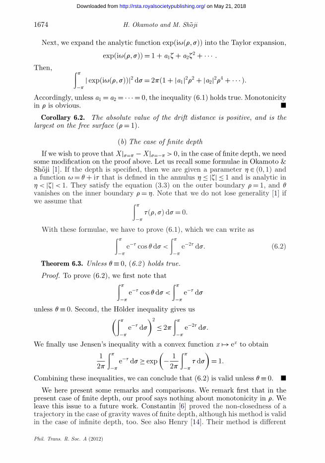
Next, we expand the analytic function exp(iu(r, s)) into the Taylor expansion,

exp(iu(r, s)) = 1 + a1z + a2z2 + · · · .

Then, ∫p

−p

| exp(iu(r, s))|2 ds = 2p(1 + |a1|2r2 + |a2|2r4 + · · · ).

Accordingly, unless a1 = a2 = · · · = 0, the inequality (6.1) holds true. Monotonicityin r is obvious. �

Corollary 6.2. The absolute value of the drift distance is positive, and is thelargest on the free surface (r = 1).

(b) The case of finite depth

If we wish to prove that X |s=p − X |s=−p > 0, in the case of finite depth, we needsome modification on the proof above. Let us recall some formulae in Okamoto &Shoji [1]. If the depth is specified, then we are given a parameter h ∈ (0, 1) anda function u = q + it that is defined in the annulus h ≤ |z| ≤ 1 and is analytic inh < |z| < 1. They satisfy the equation (3.3) on the outer boundary r = 1, and qvanishes on the inner boundary r = h. Note that we do not lose generality [1] ifwe assume that ∫p

−p

t(r, s) ds = 0.

With these formulae, we have to prove (6.1), which we can write as∫p

−p

e−t cos q ds <

∫p

−p

e−2t ds. (6.2)

Theorem 6.3. Unless q ≡ 0, (6.2 ) holds true.

Proof. To prove (6.2), we first note that∫p

−p

e−t cos q ds <

∫p

−p

e−t ds

unless q ≡ 0. Second, the Hölder inequality gives us(∫p

−p

e−t ds

)2

≤ 2p

∫p

−p

e−2t ds.

We finally use Jensen’s inequality with a convex function x → ex to obtain

12p

∫p

−p

e−t ds ≥ exp(

− 12p

∫p

−p

t ds

)= 1.

Combining these inequalities, we can conclude that (6.2) is valid unless q ≡ 0. �We here present some remarks and comparisons. We remark first that in the

present case of finite depth, our proof says nothing about monotonicity in r. Weleave this issue to a future work. Constantin [6] proved the non-closedness of atrajectory in the case of gravity waves of finite depth, although his method is validin the case of infinite depth, too. See also Henry [14]. Their method is different





from ours. Ours is also valid in the presence of surface tension. It seems to us thatthe proof in earlier studies [6,14] requires an assumption that the wave profile hasone and only one relative maximum. We do not need to assume this. As numericalexamples of gravity waves that possess more than one relative maxima in itsprofile are known [1], our proof may be worth being recorded. (The capillary–gravity waves in §5 are also such examples.) A theorem in the case of solitarywaves was considered by Constantin & Escher [12].

Water waves with underlying uniform current are considered in Constantin &Strauss [13]. We can also consider them with underlying shear flow, seeOkamoto & Shoji [1, ch. 7]. These constitute further problems, but we leavethem to the reader.

7. Conclusion

None of the particle trajectories in the stationary coordinates are closed, althoughthey are very close to a closed circular curve if the fluid particle lies deeply. Fluidparticles are pushed out by the wave in the same direction as the wave. Thedrift distance is the largest on the water surface and decreases exponentially andmonotonically in depth.

As Gerstner’s wave has been a unique example of explicitly written trajectories,our explicit formula for particle trajectory of Crapper’s waves may be worthy ofnotice. This analysis can be viewed as one of the particle dynamics considered inmany situations in earlier studies [25,26].

We are naturally led to a question: if we consider a rotational wave, what isa necessary and sufficient condition for a vorticity distribution to produce closedtrajectories only? Our method is restricted to irrotational waves, and does notseem to work in the case of rotational waves. For rotational waves, see Okamoto &Shoji [1, ch. 7] and other recent papers [19,20,22,27–29]. Waves on a slopingbeach [21], too, may well give us an interesting problem. We would like to posethis problem to the reader.

This work was inspired by A. Constantin’s seminar talk in Kyoto University. His comments onthe early version of our manuscript are acknowledged with deep gratitude. Also, comments of twoanonymous referees were valuable in revising this paper. Partially supported by JSPS grant no.20244006.

References

1 Okamoto, H. & Shoji, M. 2001 The mathematical theory of bifurcation of permanent progressivewater-waves. Singapore: World Scientific.

2 Longuett-Higgins, M. S. 1979 The trajectories of particles in deep, symmetric gravity waves.J. Fluid Mech. 94, 497–517. (doi:10.1017/S0022112079001154)

3 Lamb, H. 1932 Hydrodynamics. Cambridge, UK: Cambridge University Press.4 Milne-Thomson, L. M. 1968 Theoretical hydrodynamics, 5th edn. London, UK: Macmillan.5 Stokes, G. G. 1847 On the theory of oscillatory waves. Trans. Camb. Phil. Soc. 8; Math. Phys.

Pap. 1, 197–229. (doi:10.1017/CBO9780511702242.013)6 Constantin, A. 2006 The trajectories of particles in Stokes waves. Invent. Math. 166, 523–535.

(doi:10.1007/s00222-006-0002-5)7 Constantin, A., Ehrnström, M. & Villari, G. 2008 Particle trajectories in linear deep-water

waves. Nonlin. Anal. Real World Appl. 9, 1336–1344. (doi:10.1016/j.nonrwa.2007.03.003)



http://dx.doi.org/doi:10.1017/S0022112079001154

http://dx.doi.org/doi:10.1017/CBO9780511702242.013

http://dx.doi.org/doi:10.1007/s00222-006-0002-5

http://dx.doi.org/doi:10.1016/j.nonrwa.2007.03.003



8 Constantin, A. & Villari, G. 2008 Particle trajectories in linear water waves. J. Math. FluidMech. 10, 1–18. (doi:10.1007/s00021-005-0214-2)

9 Craik, A. D. D. 2004 The origin of water wave theory. Ann. Rev. Fluid Mech. 36, 1–28.(doi:10.1146/annurev.fluid.36.050802.122118)

10 Green, G. 1871 Note on the motion of waves in canals. In Mathematical papers by George Green(ed. N. M. Ferrers), pp. 273–280. London, UK: Macmillan.

11 Van Dyke, M. 1982 An album of fluid motion. Stanford, CA: Parabolic Press.12 Constantin, A. & Escher, J. 2007 Particle trajectories in solitary water waves. Bull. Am. Math.

Soc. 44, 423–431. (doi:10.1090/S0273-0979-07-01159-7)13 Constantin, A. & Strauss, W. 2010 Pressure beneath a Stokes wave. Commun. Pure Appl.

Math. 63, 533–557. (doi:10.1002/cpa.20299)14 Henry, D. 2006 The trajectories of particles in deep-water Stokes waves. Int. Math. Res. Notices

2006, 1–13.15 Chen, Y.-Y., Hsu, H.-C. & Chen, G.-Y. 2010 Lagrangian experiment and solution for

irrotational finite-amplitude progressive gravity waves at uniform depth. Fluid Dyn. Res. 42,045511. (doi:10.1088/0169-5983/42/4/045511)

16 Umeyama, M. 2010 Coupled PIV and PTV measurements of particle velocities and trajectoriesfor surface waves following a steady current. J. Waterw. Port Coast. Ocean Eng. 137, 85–94.(doi:10.1061/(ASCE)WW.1943-5460.0000067)

17 Gerstner, F. 1809 Theorie der Wellen. Ann. Phys. 32, 412–445. (doi:10.1002/andp.18090320808)18 Rankine, W. J. M. 1863 On the exact form of waves near the surface of deep water. Phil. Trans.

R. Soc. Lond. 153, 127–138. (10.1098/rstl.1863.0006)19 Constantin, A. 2001 On the deep water wave motion. J. Phys. A 34, 1405–1417. (doi:10.1088/

0305-4470/34/7/313)20 Henry, D. 2008 On Gerstner’s water wave. J. Nonlin. Math. Phys. 15, 87–95. (doi:10.2991/

jnmp.2008.15.s2.7)21 Constantin, A. 2001 Edge waves along a sloping beach. J. Phys. A 34, 9723–9731. (doi:10.1088/

0305-4470/34/45/311)22 Constantin, A. & Escher, J. 2011 Analyticity of periodic traveling free surface water waves with

vorticity. Ann. Math. 173, 559–568. (doi:10.4007/annals.2011.173.1.12)23 Toland, J. F. 1996 Stokes waves. Topol. Meth. Nonlinear Anal. 7, 1–48.24 Crapper, G. D. 1957 An exact solution for progressive capillary waves of arbitrary amplitude.

J. Fluid Mech. 2, 532–540. (doi:10.1017/S0022112057000348)25 Kimura, Y. & Koikari, S. 2004 Particle transport by a vortex soliton. J. Fluid Mech. 510,

201–218. (doi:10.1017/S0022112004009383)26 Shoji, M., Okamoto, H. & Ooura, T. 2010 Particle trajectories around a running cylinder or a

sphere. Fluid Dyn. Res. 42, 025506. (doi:10.1088/0169-5983/42/2/025506)27 Constantin, A. & Varvaruca, E. 2011 Steady periodic water waves with constant vorticity:

regularity and local bifurcation. Arch. Rational Mech. Anal. 199, 33–67. (doi:10.1007/s00205-010-0314-x)

28 Ehrnström, M. & Villari, G. 2008 Linear water waves with vorticity: rotational features andparticle paths. J. Differ. Equ. 244, 1888–1909. (doi:10.1016/j.jde.2008.01.012)

29 Wahlen, E. 2009 Steady water waves with a critical layer. J. Differ. Equ. 246, 2468–2483.(doi:10.1016/j.jde.2008.10.005)



http://dx.doi.org/doi:10.1007/s00021-005-0214-2

http://dx.doi.org/doi:10.1146/annurev.fluid.36.050802.122118

http://dx.doi.org/doi:10.1090/S0273-0979-07-01159-7

http://dx.doi.org/doi:10.1002/cpa.20299

http://dx.doi.org/doi:10.1088/0169-5983/42/4/045511

http://dx.doi.org/doi:10.1061/(ASCE)WW.1943-5460.0000067

http://dx.doi.org/doi:10.1002/andp.18090320808

http://dx.doi.org/10.1098/rstl.1863.0006



http://dx.doi.org/doi:10.2991/jnmp.2008.15.s2.7

http://dx.doi.org/doi:10.2991/jnmp.2008.15.s2.7



http://dx.doi.org/doi:10.4007/annals.2011.173.1.12




http://dx.doi.org/doi:10.1007/s00205-010-0314-x

http://dx.doi.org/doi:10.1007/s00205-010-0314-x

http://dx.doi.org/doi:10.1016/j.jde.2008.01.012

http://dx.doi.org/doi:10.1016/j.jde.2008.10.005


trajectories of ﬂuid particles in a periodic water...

Documents