analysis of stokes flow through periodic permeable … · bessel function abstract this ......

Alexandria Engineering Journal (2016) xxx, xxx–xxx

HO ST E D BY

Alexandria University

Alexandria Engineering Journal

www.elsevier.com/locate/aejwww.sciencedirect.com

ORIGINAL ARTICLE

Analysis of Stokes flow through periodic permeable

tubules

* Corresponding author.

Peer review under responsibility of Faculty of Engineering, Alexandria

University.

http://dx.doi.org/10.1016/j.aej.2016.09.0101110-0168 � 2016 Faculty of Engineering, Alexandria University. Production and hosting by Elsevier B.V.This is an open access article under the CC BY-NC-ND license (http://creativecommons.org/licenses/by-nc-nd/4.0/).

Please cite this article in press as: A.M. Siddiqui et al., Analysis of Stokes flow through periodic permeable tubules, Alexandria Eng. J. (2016), http://dx10.1016/j.aej.2016.09.010

A.M. Siddiqui a, Ayesha Sohail b,*, S. Naqvi c, T. Haroon d

aDepartment of Mathematics, Pennsylvania State University, York Campus, Edgecomb Avenue, PA 1703, USAbDepartment of Mathematics, COMSATS Institute of Information Technology, Lahore 54000, PakistancDepartment of Mathematics, COMSATS Institute of Information Technology, Attock, PakistandDepartment of Mathematics, COMSATS Institute of Information Technology, Islamabad 44000, Pakistan

Received 15 August 2016; revised 19 September 2016; accepted 20 September 2016

KEYWORDS

Stokes flow;

Permeable tube;

Periodic penetration;

Bessel function

Abstract This article reports the detailed analysis of the Stokes flow through permeable tubes. The

objective of this investigation was to search for exact solutions to the Stokes flow and thereby

observe the effects on radial flow component, provided the permeability on the tubular surface is

an elementary trigonometric function. Mathematical expressions for the pressure distribution,

velocity components, volume flux, average wall shear stress and leakage flux are presented explic-

itly. Graphical analysis of the fluid flow is presented for a set of parametric values. Important con-

clusions are drawn for Stokes flow through tubes with low as well as high permeability. The classical

Poiseuille flow is presented as a limiting case of this immense study of Stokes flow.� 2016 Faculty of Engineering, Alexandria University. Production and hosting by Elsevier B.V. This is an

open access article under the CC BY-NC-ND license (http://creativecommons.org/licenses/by-nc-nd/4.0/).

1. Introduction

Detailed analysis of Stokes flow is of great significance due toits importance in biological and industrial studies. Fluid flowwhich is dominated by viscosity i.e., Reynolds number,

Re� 1, is quite suitably called Stokes flow (or creeping flow),and such fluids do not make spinning vortices or become tur-bulent, but rather ooze or creep around obstacles. Vast litera-

ture is available on the analysis of Stokes flow [1–7].The human body possesses the Poiseuille stokes flow; for

example, the heart requires the pressure to pump the bloodin arteriole. An arteriole is the branching off of an artery with

significantly lower blood pressures, and they are the portions

of arteries that deliver blood directly to the tissues at Reynolds

number around 0.7. Therefore Stokes flow analysis is of inter-est in physiology with regard to fluid transport from capillarytubes into surrounding tissue. A few dozen liters of biological

fluid perfuse through the capillaries of the human body eachday.

The hydrodynamics of the proximal renal tubule [8] andblood perfusion through kidneys (organic and artificial

hollow-fiber) [9] are examples of Stokes flow. The blood flowsinto the mammalian kidneys through the renal artery andenters the glomerulus in Bowman’s capsule. In the glomerulus,

the blood flow is split into fifty capillaries that have very thinwalls. The solutes in the blood are easily filtered through thesewalls due to the pressure gradient that exists between the blood

in the capillaries and the fluid in the Bowman’s capsule. Thepressure gradient is controlled by the contraction or dilationof the arterioles. After passing through the afferent arteriole,

.doi.org/

http://creativecommons.org/licenses/by-nc-nd/4.0/

http://dx.doi.org/10.1016/j.aej.2016.09.010


http://www.sciencedirect.com/science/journal/11100168


http://creativecommons.org/licenses/by-nc-nd/4.0/



Figure 1 Stokes flow through tube with periodic boundaries.

2 A.M. Siddiqui et al.

the filtered blood enters the vasa recta. Blood exits the kidneysthrough the renal vein. Recently, Haroon et al. [10] studied theStokes flow of an incompressible viscous fluid through a slit

with periodic reabsorption at the walls. They showed thatthe periodic reabsorption parameter plays a dominant role inaltering the flow properties, which are useful in analyzing flow

behavior during the reabsorption. Ahmad and Ahmad [20]studied the blood flow through renal tubules in detail but therecalculations did not fully demonstrate the flow behavior.

Industrial applications of flow through permeable tubes areencountered in desalination, flow through tubular nano-structures [11–14] and reverse osmosis. Clear understandingof osmosis and filtration is of notable importance. These two

processes take place by pumping the fluid to be filteredthrough porous walled ducts at elevated pressure.

Keeping in view the significance of the Stokes flow analysis

in tube geometry in biological systems and in industry, thiswork demonstrates the pressure-driven Stokes flow throughpermeable tube with periodic permeation. In order to develop

a more balanced model of the problem while evading the com-plications (accuracy, computational cost, etc.) of a fully three-dimensional computation, we have examined the two-

dimensional equivalent of the penetrable tube problem forReynolds number (Re < 1), in which the walls are consideredto be porous membrane with periodic boundary condition.The motive of this research is to present a collective study of

the cases presented in the literature [16] and the referencestherein. The periodic permeation is considered and the classicalPoiseuille flow properties are retrieved as limiting case without

periodic permeation. Two important aspects will be targetedduring this research: (i) the link between the volume flow rateand the velocity profiles, and (ii) the penetration rate and the

velocity profile. This will help to understand the models (Engi-neering [17,18] and biological [19]) of the filtration processes.We will present the mathematical model in the next section,

and Section 3 presents the detailed derivation of the pressuredistribution, velocity components and volume flux rate. In Sec-tion 4, we have presented the flow profile with the aid of thevideo-graphic footage. Finally, we have discussed the results

and have listed the important conclusions.

2. Problem formulation and mathematical modeling

Consider the steady, laminar, fully developed, isothermal flowof an incompressible Newtonian fluid passing through perme-able narrow tube of radius R and length L which is homoge-

neous to the flow model as shown in the schematic diagramFig. 1. Here we choose the axisymmetric coordinate accordingto the geometry of problem. The z-axis of the tube is taken

along the axis of the tube (transverse axis) and r, the radial-axis is perpendicular to it.

Under the assumption that the flow is symmetric about thez-axis, we pursue that the velocity profile is governed by the

following set of equations:

v ¼ vr r; zð Þ; vz r; zð Þ½ �; ð1ÞSince our motive is to study the creeping flow, the inertial termcan be neglected. Using this assumption the Navier-Stokes

equation takes the form of

1

r

@

@rrvrð Þ þ @vz

@z¼ 0; ð2Þ

Please cite this article in press as: A.M. Siddiqui et al., Analysis of Stokes flow thro10.1016/j.aej.2016.09.010

@p

@r¼ l

@2vr@r2

þ 1

r

@vr@r

� vrr2þ @2vr

@z2

� �ð3Þ

@p

@z¼ l

@2vz

@r2þ 1

r

@vz@r

þ @2vz@z2

� �ð4Þ

The boundary conditions are given as

vr ¼ 0 at r ¼ 0; ð5Þ@vz@r

¼ 0 at r ¼ 0; ð6Þ

vr ¼vo sin az case1ð Þvo cos az case2ð Þ

�at r ¼ R; ð7Þ

vz ¼ 0 at r ¼ R; ð8Þ

2pZ R

0

rvz r; 0ð Þdr ¼ Qo at z ¼ 0: ð9Þ

p ¼ p0 at z ¼ 0; ð10Þp ¼ pL at z ¼ L; ð11Þwhere vo is the uniform suction velocity at z ¼ p

2a for the case1

and z ¼ 0 for the case2. a is the periodic suction parameter.In a manner similar to Macey [15], eliminating the pressure

from Eqs. (3) and (4) and utilizing Eq. (2) we obtain

ugh periodic permeable tubules, Alexandria Eng. J. (2016), http://dx.doi.org/



0 0.5 1 1.5 2−1

−0.8

−0.6

−0.4

−0.2

0

0.2

0.4

0.6

0.8

1

vz(r,z)

r

Q0 = 1,3,5

v0 = 0 at r = R

−0.5 0 0.5 1 1.5 2−1

−0.8

−0.6

−0.4

−0.2

0

0.2

0.4

0.6

0.8

1

vz(r,z)

r

Q0 = 1,3,5

v0 = v

0sin(αz) at r = R

0 0.5 1 1.5 2 2.5 3 3.5 4 4.5 5−1

−0.8

−0.6

−0.4

−0.2

0

0.2

0.4

0.6

0.8

1

vz(r,z)

r

Q0 = 1,3,5

v0 = v

0cos(αz) at r = R

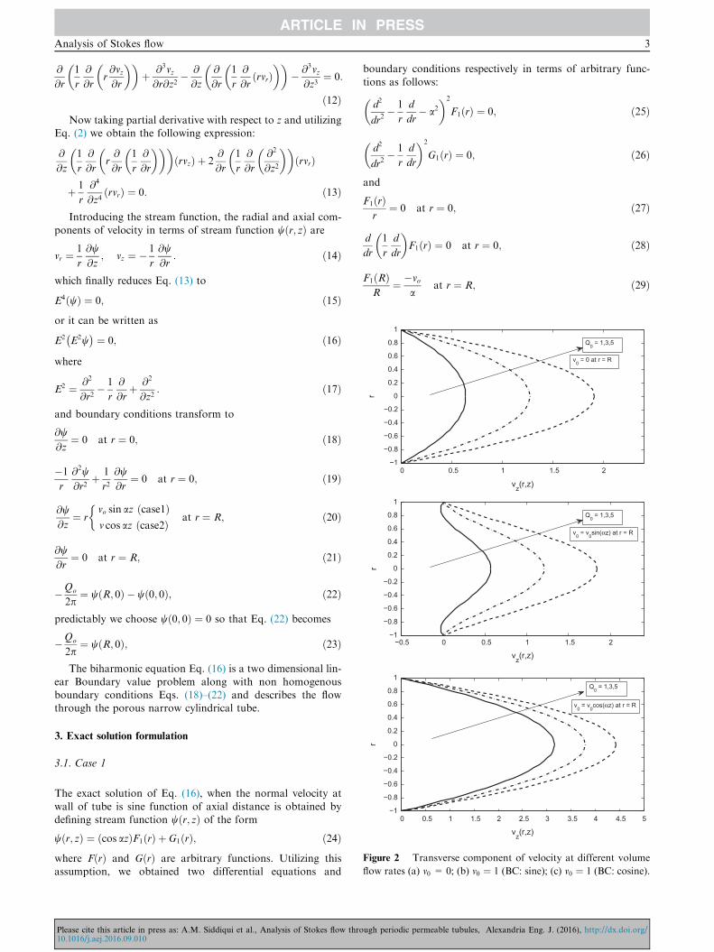
Figure 2 Transverse component of velocity at different volume

flow rates (a) v0 = 0; (b) v0 ¼ 1 (BC: sine); (c) v0 ¼ 1 (BC: cosine).

Analysis of Stokes flow 3

@

@r

1

r

@

@rr@vz@r

� �� þ @3vz@r@z2

� @

@z

@

@r

1

r

@

@rrvrð Þ

� �� @3vz

@z3¼ 0:

ð12ÞNow taking partial derivative with respect to z and utilizing

Eq. (2) we obtain the following expression:

@

@z

1

r

@

@rr@

@r

1

r

@

@r

� �� rvzð Þ þ 2

@

@r

1

r

@

@r

@2

@z2

� �� rvrð Þ

þ 1

r

@4

@z4rvrð Þ ¼ 0: ð13Þ

Introducing the stream function, the radial and axial com-

ponents of velocity in terms of stream function w r; zð Þ are

vr ¼ 1

r

@w@z

; vz ¼ � 1

r

@w@r

: ð14Þ

which finally reduces Eq. (13) to

E4ðwÞ ¼ 0; ð15Þor it can be written as

E2 E2w� � ¼ 0; ð16Þ

where

E2 ¼ @2

@r2� 1

r

@

@rþ @2

@z2: ð17Þ

and boundary conditions transform to

@w@z

¼ 0 at r ¼ 0; ð18Þ

�1

r

@2w@r2

þ 1

r2@w@r

¼ 0 at r ¼ 0; ð19Þ

@w@z

¼ rvo sin az case1ð Þv cos az case2ð Þ

�at r ¼ R; ð20Þ

@w@r

¼ 0 at r ¼ R; ð21Þ

�Qo

2p¼ w R; 0ð Þ � w 0; 0ð Þ; ð22Þ

predictably we choose w 0; 0ð Þ ¼ 0 so that Eq. (22) becomes

�Qo

2p¼ w R; 0ð Þ; ð23Þ

The biharmonic equation Eq. (16) is a two dimensional lin-

ear Boundary value problem along with non homogenousboundary conditions Eqs. (18)–(22) and describes the flowthrough the porous narrow cylindrical tube.

3. Exact solution formulation

3.1. Case 1

The exact solution of Eq. (16), when the normal velocity at

wall of tube is sine function of axial distance is obtained bydefining stream function w r; zð Þ of the form

w r; zð Þ ¼ cos azð ÞF1 rð Þ þ G1 rð Þ; ð24Þwhere F rð Þ and G rð Þ are arbitrary functions. Utilizing thisassumption, we obtained two differential equations and


boundary conditions respectively in terms of arbitrary func-

tions as follows:

d2

dr2� 1

r

d

dr� a2

� �2

F1 rð Þ ¼ 0; ð25Þ

d2

dr2� 1

r

d

dr

� �2

G1 rð Þ ¼ 0; ð26Þ

and

F1 rð Þr

¼ 0 at r ¼ 0; ð27Þ

d

dr

1

r

d

dr

� �F1 rð Þ ¼ 0 at r ¼ 0; ð28Þ

F1 Rð ÞR

¼ �voa

at r ¼ R; ð29Þ




−4 −3 −2 −1 0 1 2 3 40.5

1

1.5

2

2.5

3

3.5

4

z

v z(r,z

)

r = 0 z

r

r = 0.3

r = 0.6

vr (R,z) = v

o cos(α z)

r = 0.1

−4 −3 −2 −1 0 1 2 3 40.5

1

1.5

2

2.5

3

3.5

4

z

v z(r,z

)

r = 0 z

r

r = 0.1

r = 0.3

r = 0.6

vr (R,z) = v

o sin(α z)

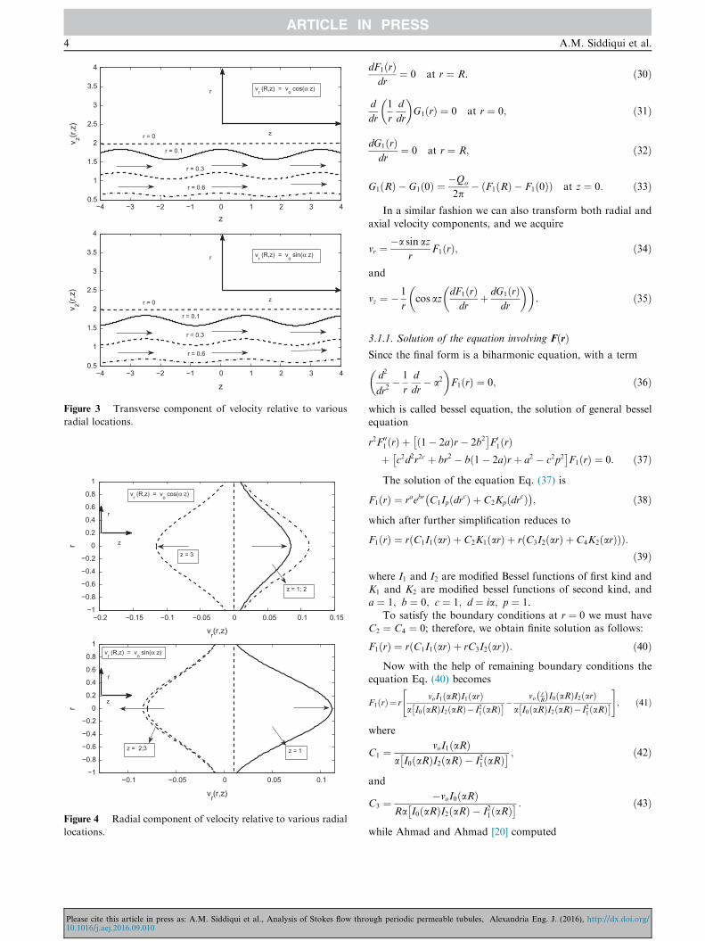
Figure 3 Transverse component of velocity relative to various

radial locations.

−0.2 −0.15 −0.1 −0.05 0 0.05 0.1 0.15−1

−0.8

−0.6

−0.4

−0.2

0

0.2

0.4

0.6

0.8

1

vr(r,z)

r z

r

vr (R,z) = v

o cos(α z)

z = 1; 2

z = 3

−0.1 −0.05 0 0.05 0.1−1

−0.8

−0.6

−0.4

−0.2

0

0.2

0.4

0.6

0.8

1

vr(r,z)

r

r

vr (R,z) = v

o sin(α z)

z = 1

z

z = 2;3

Figure 4 Radial component of velocity relative to various radial

locations.



dF1 rð Þdr

¼ 0 at r ¼ R: ð30Þ

d

dr

1

r

d

dr

� �G1 rð Þ ¼ 0 at r ¼ 0; ð31Þ

dG1 rð Þdr

¼ 0 at r ¼ R; ð32Þ

G1 Rð Þ � G1 0ð Þ ¼ �Qo

2p� F1 Rð Þ � F1 0ð Þð Þ at z ¼ 0: ð33Þ

In a similar fashion we can also transform both radial and

axial velocity components, and we acquire

vr ¼ �a sin azr

F1 rð Þ; ð34Þ

and

vz ¼ � 1

rcos az

dF1ðrÞdr

þ dG1 rð Þdr

� �� : ð35Þ

3.1.1. Solution of the equation involving F rð ÞSince the final form is a biharmonic equation, with a term

d2

dr2� 1

r

d

dr� a2

� �F1 rð Þ ¼ 0; ð36Þ

which is called bessel equation, the solution of general besselequation

r2F001 rð Þ þ 1� 2að Þr� 2b2

� �F01 rð Þ

þ c2d2r2c þ br2 � b 1� 2að Þrþ a2 � c2p2� �

F1 rð Þ ¼ 0: ð37ÞThe solution of the equation Eq. (37) is

F1 rð Þ ¼ raebr C1Ip drcð Þ þ C2Kp drcð Þ� �; ð38Þ

which after further simplification reduces to

F1 rð Þ ¼ r C1I1 arð Þ þ C2K1 arð Þ þ r C3I2 arð Þ þ C4K2 arð Þð Þð Þ:ð39Þ

where I1 and I2 are modified Bessel functions of first kind and

K1 and K2 are modified bessel functions of second kind, anda ¼ 1; b ¼ 0; c ¼ 1; d ¼ ia; p ¼ 1.

To satisfy the boundary conditions at r ¼ 0 we must haveC2 ¼ C4 ¼ 0; therefore, we obtain finite solution as follows:

F1 rð Þ ¼ r C1I1 arð Þ þ rC3I2 arð Þð Þ: ð40ÞNow with the help of remaining boundary conditions the

equation Eq. (40) becomes

F1 rð Þ¼ rvoI1 aRð ÞI1 arð Þ

a I0 aRð ÞI2 aRð Þ� I21 aRð Þ� �� vorR

� �I0 aRð ÞI2 arð Þ

a I0 aRð ÞI2 aRð Þ�I21 aRð Þ� �" #

; ð41Þ

where

C1 ¼ voI1 aRð Þa I0 aRð ÞI2 aRð Þ � I21 aRð Þ� � ; ð42Þ

and

C3 ¼ �voI0 aRð ÞRa I0 aRð ÞI2 aRð Þ � I21 aRð Þ� � : ð43Þ

while Ahmad and Ahmad [20] computed




−0.4 −0.2 0 0.2 0.4 0.6 0.8−1

−0.8

−0.6

−0.4

−0.2

0

0.2

0.4

0.6

0.8

1

vr(r,z)

rr

z

z = 0.5; 1;1.5; 2; 2.5; 3; 3.5;4

vr (R,z) = v

ocos(αz); α = 1; Q

0=1

−0.4 −0.2 0 0.2 0.4 0.6 0.8−1

−0.8

−0.6

−0.4

−0.2

0

0.2

0.4

0.6

0.8

1

vr(r,z)

r

r

z

vr (R,z) = v


0=1z = 0.5; 1;1.5; 2; 2.5; 3; 3.5;4

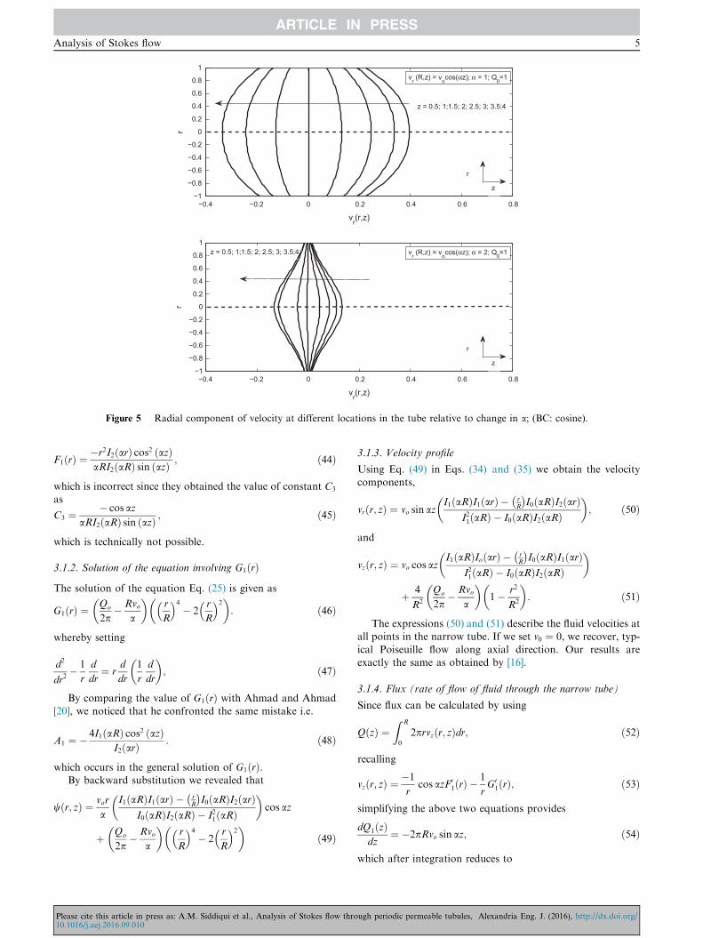
Figure 5 Radial component of velocity at different locations in the tube relative to change in a; (BC: cosine).


F1 rð Þ ¼ �r2I2 arð Þ cos2 azð ÞaRI2 aRð Þ sin azð Þ ; ð44Þ

which is incorrect since they obtained the value of constant C3

as

C3 ¼ � cos azaRI2 aRð Þ sin azð Þ ; ð45Þ

which is technically not possible.

3.1.2. Solution of the equation involving G1 rð ÞThe solution of the equation Eq. (25) is given as

G1 rð Þ ¼ Qo

2p� Rvo

a

� �r

R

4� 2

r

R

2� �: ð46Þ

whereby setting

d2

dr2� 1

r

d

dr¼ r

d

dr

1

r

d

dr

� �; ð47Þ

By comparing the value of G1ðrÞ with Ahmad and Ahmad[20], we noticed that he confronted the same mistake i.e.

A1 ¼ � 4I1 aRð Þ cos2 azð ÞI2 arð Þ : ð48Þ

which occurs in the general solution of G1 rð Þ.By backward substitution we revealed that

w r; zð Þ ¼ vor

a

I1 aRð ÞI1 arð Þ � rR


I0 aRð ÞI2 aRð Þ � I21 aRð Þ

� �cos az

þ Qo

2p� Rvo

a

� �r

R

4� 2

r

R

2� �ð49Þ


3.1.3. Velocity profile

Using Eq. (49) in Eqs. (34) and (35) we obtain the velocitycomponents,

vr r; zð Þ ¼ vo sin azI1 aRð ÞI1 arð Þ � r

R


I21 aRð Þ � I0 aRð ÞI2 aRð Þ� �

; ð50Þ

and

vz r; zð Þ ¼ vo cos azI1 aRð ÞIo arð Þ � r

R


I21 aRð Þ � I0 aRð ÞI2 aRð Þ� �

þ 4

R2

Qo

2p� Rvo

a

� �1� r2

R2

� �: ð51Þ

The expressions (50) and (51) describe the fluid velocities atall points in the narrow tube. If we set v0 ¼ 0, we recover, typ-

ical Poiseuille flow along axial direction. Our results areexactly the same as obtained by [16].

3.1.4. Flux (rate of flow of fluid through the narrow tube)

Since flux can be calculated by using

QðzÞ ¼Z R

0

2prvz r; zð Þdr; ð52Þ

recalling

vzðr; zÞ ¼ �1

rcos azF0

1 rð Þ � 1

rG0

1 rð Þ; ð53Þ

simplifying the above two equations provides

dQ1 zð Þdz

¼ �2pRvo sin az; ð54Þ

which after integration reduces to




0 0.1 0.2 0.3 0.4 0.5 0.6 0.7 0.8−1

−0.8−0.6−0.4−0.2

00.20.40.60.8

1

vr(r,z)

r

z

r

z = 0.5; 1;1.5; 2; 2.5; 3; 3.5

vr (R,z) = v

osin(αz); α = 1; Q

0=1

−0.4 −0.2 0 0.2 0.4 0.6 0.8−1

−0.8−0.6−0.4−0.2

00.20.40.60.8

1

vr(r,z)

r

z

r

vr (R,z) = v


0=4

z = 0.5; 1;1.5; 2; 2.5; 3; 3.5

−0.4 −0.2 0 0.2 0.4 0.6 0.8−1

−0.8−0.6−0.4−0.2

00.20.40.60.8

1

vr(r,z)

r

z

r

z = 0.5; 1;1.5; 2; 2.5; 3; 3.5 vr (R,z) = v


0=1

−0.4 −0.2 0 0.2 0.4 0.6 0.8−1

−0.8−0.6−0.4−0.2

00.20.40.60.8

1

vr(r,z)

r

z

r

z = 0.5; 1;1.5; 2; 2.5; 3; 3.5v

r (R,z) = v


0=4

−0.4 −0.2 0 0.2 0.4 0.6 0.8−1

−0.8−0.6−0.4−0.2

00.20.40.60.8

1

vr(r,z)

r

z

r

z = 0.5; 1;1.5; 2; 2.5; 3; 3.5 vr (R,z) = v


0=1

−0.4 −0.2 0 0.2 0.4 0.6 0.8−1

−0.8−0.6−0.4−0.2

00.20.40.60.8

1

vr(r,z)

r

z

r

z = 0.5; 1;1.5; 2; 2.5; 3; 3.5v

r (R,z) = v


0=4

Figure 6 Radial component of velocity at different locations in the tube relative to change in a (Left Q0 = 1; Right Q0 ¼ 4) (BC: sine).


Q1 zð Þ ¼ Qo þ2pRvo

acos az� 1ð Þ: ð55Þ

3.1.5. Maximum axial velocity

With the help of Eq. (50) the maximum axial velocity can beobtained as

vmax ¼ vo �1ð Þm I1 aRð ÞIo arð Þ � rR


I21 aRð Þ � I0 aRð ÞI2 aRð Þ

� �

� 4

R2

Qo

2p� Rvo

a

� �1� r2

R2

� �; m 2 Zþ; ð56Þ

at the center of the tube at

z ¼ npa

8 na2 Z; a > 0:

It is clear from Eq. (56) that

(1) if n is negative then z < 0,(2) if n is positive then z > 0.

Since z is positive i.e. 0 to L then we must have positive n.


3.1.6. Pressure distribution

Utilizing Eqs. (3) and (4) we obtain

1

l@p

@r¼ 1

r

@

@zE2w� �

; ð57Þ

1

l@p

@z¼ � 1

r

@

@rE2w� �

; ð58Þ

where a straightforward computation reveals that

E2w ¼ cos azd2

dr2� 1

r

d

dr� a2

� �F1 rð Þ

þ d2

dr2� 1

r

d

dr

� �G1 rð Þ: ð59Þ

By eliminating the pressure gradient from Eqs. (57) and(58), we get

1

lp r; zð Þ ¼ � sin az

2voIo aRð ÞIo arð ÞR I0 aRð ÞI2 aRð Þ � I21 aRð Þ� �

!

� 16

R4

Qo

2p� Rvo

a

� �zþ po

l: ð60Þ




−4 −3 −2 −1 0 1 2 3 4−0.1

0

0.1

0.2

0.3

0.4

0.5

0.6

0.7

z

v z(r,z

)

z

r

r = 0.05; 0.1;0.15; 0.2; 0.25; 0.3; 0.35;0.4

vr (R,z) = v


0=1

−4 −3 −2 −1 0 1 2 3 4−1

−0.5

0

0.5

1

1.5

2

2.5

3

z

v z(r,z

)

r = 0.05; 0.1;0.15; 0.2; 0.25; 0.3; 0.35;0.4z

r

vr (R,z) = v


0=4

−4 −3 −2 −1 0 1 2 3 40

0.1

0.2

0.3

0.4

0.5

0.6

0.7

z

v z(r,z

)

z

r

r = 0.05; 0.1;0.15; 0.2; 0.25; 0.3; 0.35;0.4

vr (R,z) = v


0=1

−4 −3 −2 −1 0 1 2 3 4−1

−0.5

0

0.5

1

1.5

2

2.5

3

z

zv(r

,z)

r = 0.05; 0.1;0.15; 0.2; 0.25; 0.3; 0.35;0.4z

r

vr (R,z) = v


0=4

−4 −3 −2 −1 0 1 2 3 4−0.2−0.1

00.10.20.30.40.50.60.70.8

z

v z(r,z

)

vr (R,z) = v


0=1

r = 0.05; 0.1;0.15; 0.2; 0.25; 0.3; 0.35;0.4z

r

−4 −3 −2 −1 0 1 2 3 4−1

−0.50

0.51

1.52

2.53

3.54

z

v z(r,z

)

r = 0.05; 0.1;0.15; 0.2; 0.25; 0.3; 0.35;0.4z

r

vr (R,z) = v


0=4

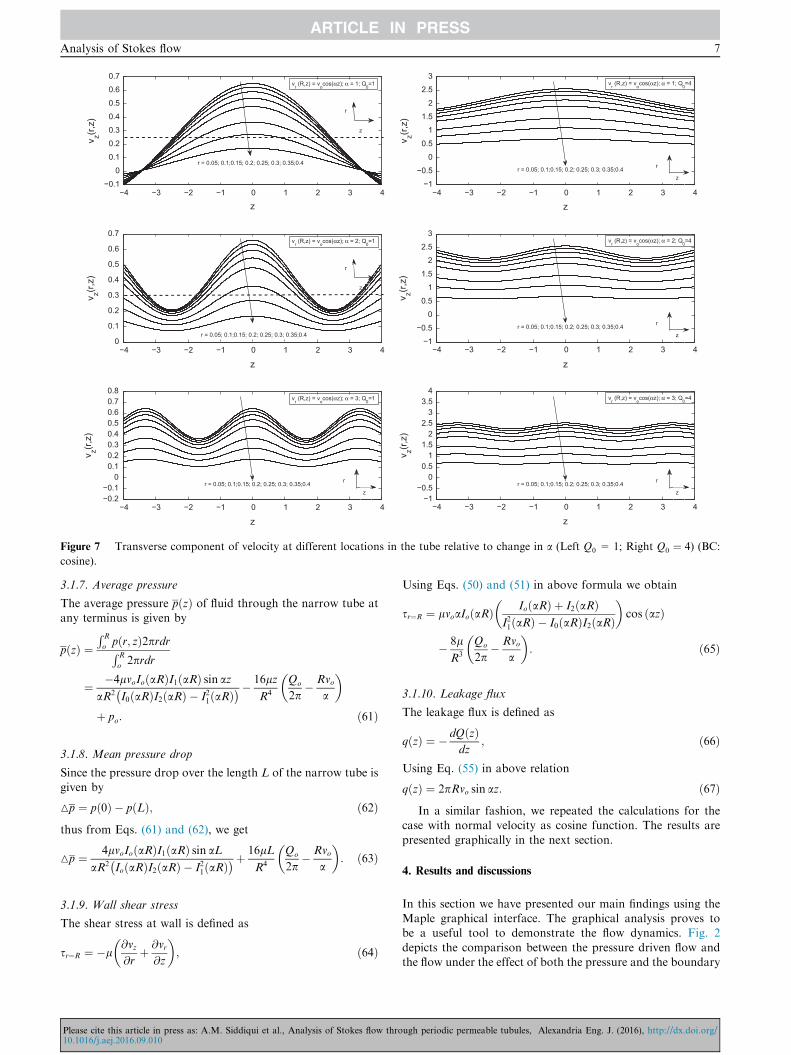
Figure 7 Transverse component of velocity at different locations in the tube relative to change in a (Left Q0 = 1; Right Q0 ¼ 4) (BC:

cosine).


3.1.7. Average pressure

The average pressure p zð Þ of fluid through the narrow tube atany terminus is given by

p zð Þ ¼R R

op r; zð Þ2prdrR R

o2prdr

¼ �4lvoIo aRð ÞI1 aRð Þ sin azaR2 I0 aRð ÞI2 aRð Þ � I21 aRð Þ� �� 16lz

R4

Qo

2p� Rvo

a

� �

þ po: ð61Þ

3.1.8. Mean pressure drop

Since the pressure drop over the length L of the narrow tube isgiven by

Mp ¼ p 0ð Þ � p Lð Þ; ð62Þthus from Eqs. (61) and (62), we get

Mp ¼ 4lvoIo aRð ÞI1 aRð Þ sin aLaR2 Io aRð ÞI2 aRð Þ � I21 aRð Þ� �þ 16lL

R4

Qo

2p� Rvo

a

� �: ð63Þ

3.1.9. Wall shear stress

The shear stress at wall is defined as

sr¼R ¼ �l@vz@r

þ @vr@z

� �; ð64Þ


Using Eqs. (50) and (51) in above formula we obtain

sr¼R ¼ lvoaIo aRð Þ Io aRð Þ þ I2 aRð ÞI21 aRð Þ � I0 aRð ÞI2 aRð Þ� �

cos azð Þ

� 8l

R3

Qo

2p� Rvo

a

� �: ð65Þ

3.1.10. Leakage flux

The leakage flux is defined as

q zð Þ ¼ � dQ zð Þdz

; ð66Þ

Using Eq. (55) in above relation

q zð Þ ¼ 2pRvo sin az: ð67ÞIn a similar fashion, we repeated the calculations for the

case with normal velocity as cosine function. The results are

presented graphically in the next section.

4. Results and discussions

In this section we have presented our main findings using theMaple graphical interface. The graphical analysis proves tobe a useful tool to demonstrate the flow dynamics. Fig. 2

depicts the comparison between the pressure driven flow andthe flow under the effect of both the pressure and the boundary




−4 −3 −2 −1 0 1 2 3 4−1

−0.8−0.6−0.4−0.2

00.20.40.60.8

1

z

v z(r,z

)

z

rr = 0.05; 0.1;0.15; 0.2; 0.25; 0.3; 0.35;0.4

vr (R,z) = v


0=1

−4 −3 −2 −1 0 1 2 3 40

0.5

1

1.5

2

2.5

3

z

zv(r

,z)

r

z

vr (R,z) = v


0=4

r = 0.05; 0.1;0.15; 0.2; 0.25; 0.3; 0.35;0.4

−4 −3 −2 −1 0 1 2 3 4

−0.2

0

0.2

0.4

0.6

0.8

z

v z(r,z

)

rr = 0.05; 0.1;0.15; 0.2; 0.25; 0.3; 0.35;0.4

vr (R,z) = v


0=1

z

−4 −3 −2 −1 0 1 2 3 4

0

0.5

1

1.5

2

2.5

3

z

v z(r,z

)

r

zr = 0.05; 0.1;0.15; 0.2; 0.25; 0.3; 0.35;0.4

vr (R,z) = v


0=4

−4 −3 −2 −1 0 1 2 3 4

−0.2

0

0.2

0.4

0.6

0.8

z

v z(r,z

)

r

z

r = 0.05; 0.1;0.15; 0.2; 0.25; 0.3; 0.35;0.4

vr (R,z) = v


0=1

−4 −3 −2 −1 0 1 2 3 4−0.5

0

0.5

1

1.5

2

2.5

3

z

v z(r,z

)

r

zr = 0.05; 0.1;0.15; 0.2; 0.25; 0.3; 0.35;0.4

vr (R,z) = v


0=4

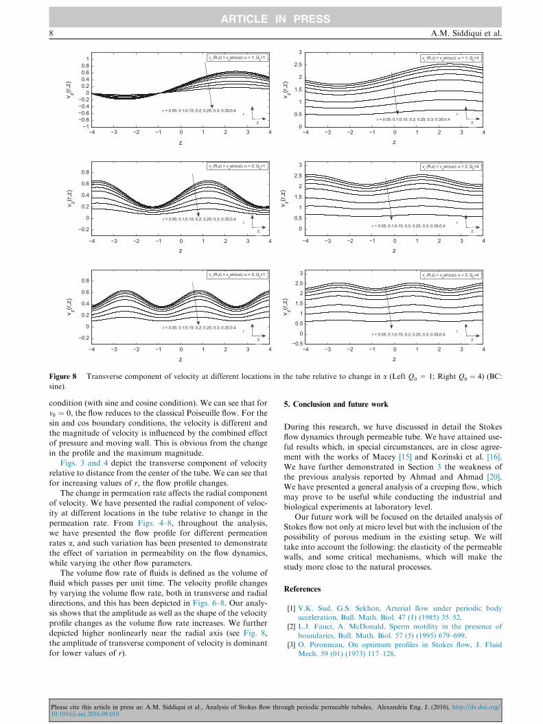
Figure 8 Transverse component of velocity at different locations in the tube relative to change in a (Left Q0 = 1; Right Q0 ¼ 4) (BC:

sine).


condition (with sine and cosine condition). We can see that forv0 ¼ 0, the flow reduces to the classical Poiseuille flow. For the

sin and cos boundary conditions, the velocity is different andthe magnitude of velocity is influenced by the combined effectof pressure and moving wall. This is obvious from the change

in the profile and the maximum magnitude.Figs. 3 and 4 depict the transverse component of velocity

relative to distance from the center of the tube. We can see that

for increasing values of r, the flow profile changes.The change in permeation rate affects the radial component

of velocity. We have presented the radial component of veloc-ity at different locations in the tube relative to change in the

permeation rate. From Figs. 4–8, throughout the analysis,we have presented the flow profile for different permeationrates a, and such variation has been presented to demonstrate

the effect of variation in permeability on the flow dynamics,while varying the other flow parameters.

The volume flow rate of fluids is defined as the volume of

fluid which passes per unit time. The velocity profile changesby varying the volume flow rate, both in transverse and radialdirections, and this has been depicted in Figs. 6–8. Our analy-sis shows that the amplitude as well as the shape of the velocity

profile changes as the volume flow rate increases. We furtherdepicted higher nonlinearly near the radial axis (see Fig. 8,the amplitude of transverse component of velocity is dominant

for lower values of r).


5. Conclusion and future work

During this research, we have discussed in detail the Stokes

flow dynamics through permeable tube. We have attained use-ful results which, in special circumstances, are in close agree-ment with the works of Macey [15] and Kozinski et al. [16].

We have further demonstrated in Section 3 the weakness ofthe previous analysis reported by Ahmad and Ahmad [20].We have presented a general analysis of a creeping flow, whichmay prove to be useful while conducting the industrial and

biological experiments at laboratory level.Our future work will be focused on the detailed analysis of

Stokes flow not only at micro level but with the inclusion of the

possibility of porous medium in the existing setup. We willtake into account the following: the elasticity of the permeablewalls, and some critical mechanisms, which will make the

study more close to the natural processes.

References

[1] V.K. Sud, G.S. Sekhon, Arterial flow under periodic body

acceleration, Bull. Math. Biol. 47 (1) (1985) 35–52.

[2] L.J. Fauci, A. McDonald, Sperm motility in the presence of

boundaries, Bull. Math. Biol. 57 (5) (1995) 679–699.

[3] O. Pironneau, On optimum profiles in Stokes flow, J. Fluid

Mech. 59 (01) (1973) 117–128.


http://refhub.elsevier.com/S1110-0168(16)30277-0/h0005









[4] T.W. Lowe, T.J. Pedley, Computation of Stokes flow in a

channel with a collapsible segment, J. Fluids Struct. 9 (8) (1995)

885–905.

[5] J. Lighthill, Flagellar hydrodynamics, SIAM Rev. 18 (2) (1976)

161–230.

[6] S.W. Walker, The Shape of Things: A Practical Guide to

Differential Geometry and the Shape Derivative, vol. 28, SIAM,

2015.

[7] T. Chacon Rebollo, V. Girault, F. Murat, O. Pironneau,

Analysis of a coupled fluid-structure model with applications

to hemodynamics, SIAM J. Numer. Anal. 54 (2) (2016) 994–

1019.

[8] E.A. Marshall, E.A. Trowbridge, Flow of a Newtonian fluid

through a permeable tube: the application to the proximal renal

tubule, Bull. Math. Biol. 36 (5–6) (1974) 457–476.

[9] S.M. Ross, A mathematical model of mass transport in a long

permeable tube with radial convection, J. Fluid Mech. 63 (01)

(1974) 157–175.

[10] T. Haroon, A.M. Siddiqui, A. Shahzad, Stokes flow through a

slit with periodic reabsorption: an application to renal tubule,

Alexandria Eng. J. (2016).

[11] G. Liu, K. Wang, N. Hoivik, H. Jakobsen, Progress on free-

standing and flow-through TiO2 nanotube membranes, Sol.

Energy Mater. Solar Cells 98 (2012) 24–38.

[12] M. Sheikholeslami, M. Azimi, D.D. Ganji, Application of

differential transformation method for nanofluid flow in a semi-


permeable channel considering magnetic field effect, Int. J.

Comput. Methods Eng. Sci. Mech. 16 (4) (2015) 246–255.

[13] M. Sheikholeslami, M.M. Rashidi, T. Hayat, D.D. Ganji, Free

convection of magnetic nanofluid considering MFD viscosity

effect, J. Mol. Liq. 218 (2016) 393–399.

[14] M. Sheikholeslami, D.D. Ganji, M.Y. Javed, R. Ellahi, Effect of

thermal radiation on magnetohydrodynamics nanofluid flow

and heat transfer by means of two phase model, J. Magn. Magn.

Mater. 374 (2015) 36–43.

[15] R.I. Macey, Pressure flow patterns in a cylinder with

reabsorbing walls, Bull. Math. Biophys. 25 (1963) 1–9.

[16] A.A. Kozinski, F.P. Schmidt, E.N. Lightfoot, Velocity profiles

in porous-walled ducts, Ind. Eng. Chem. Fundam. 9 (3) (1970)

502–505.

[17] E.S. Mickaily, S. Middleman, M. Allen, Viscous flow over

periodic surfaces, Chem. Eng. Commun. 117 (1) (1992) 401–414.

[18] M. Heil, Stokes flow in an elastic tube—a large displacement

fluid structure interaction problem, Int. J. Numer. Methods

Fluids 28 (2) (1998) 243–265.

[19] S. Vogel, Life in Moving Fluids: The Physical Biology of Flow,

Princeton University Press, 1994.

[20] S. Ahmad, N. Ahmad, On flow through renal tubule in case of

periodic radial velocity component, Int. J. Emerg. Multidiscip.

Fluid Sci. 3 (4) (2011) 201–208.
























































analysis of stokes flow through periodic permeable … · bessel function abstract this ......

Documents