training effectiveness of flight simulators with outside ... · adquirem aptido˜es de pilotagem...

Training Effectiveness of Flight Simulatorswith Outside Visual Cues

Miguel Freitas da Silva Mendes

Thesis to obtain the Master of Science Degree in

Aerospace Engineering

Supervisor: Prof. Agostinho Rui Alves da Fonseca

Examination Committee

Chairperson: Prof. João Manuel Lage de Miranda Lemos

Supervisor: Prof. Agostinho Rui Alves da Fonseca

Member of the Committee: Prof. José Raúl Carreira Azinheira

October 28, 2016

Acknowledgments

Conducting a research project like the one behind this dissertation was something I looked

forward to ever since I started my academic path, back in 2010. When choosing my Grad-

uation Project to obtain the Master degree on the Aerospace Engineering Faculty at Delft

University of Technology, this topic was proposed by my thesis advisor dr.ir. Daan Pool and

to him I must dedicate the first acknowledgment of this work. The door of dr.ir. Pool’s office

was always opened whenever I ran into a trouble during the last 7 months and his consistent

guidance and immense knowledge and experience were fundamental to elaborate this work.

I must also thank to senior researcher engineer Peter Zaal, of the NASA Ames Research

Center at San Jose State University, for his availability to steer me in the right direction with

his fruitful and insightful inputs given in several moments of the work developed.

I would further like to express a note of gratefulness to the 22 people who volunteered to

perform this experiment. Their commitment to this project, with each of them spending a

total of 8 hours on the simulator, was remarkable.

On a personal level, a significant thank-you must be expressed to Joao Paulo, for his valuable

friendship and for being my travel partner in the journey this Master’s program we both

followed was. I must also dedicate the deepest appreciation note to Mariana for her crucial

presence and importance in my life. Last but definitely not least I must express my very

profound gratitude to my parents and my sister, my aunt and my grandparents, for their

continuous encouragement throughout my years of study, unfailing support, and ultimately

for providing me with this opportunity of completing my studies far from their so loved home.

Training Effectiveness of Flight Simulators with Outside Visual Cues M.F.S. Mendes

ii Acknowledgments

M.F.S. Mendes Training Effectiveness of Flight Simulators with Outside Visual Cues

Abstract

To control an aircraft, human pilots rely on their visual and somatosensory systems to perceive

their self-motion through the world and thereby control their aircraft. Nowadays, pilot acquire

such low-level control skills almost exclusively during simulator-based training. To study

this learning process and investigate the effectiveness of simulator-based training procedures,

transfer-of-training experiments are performed to evaluate from a cybernetic perspective how

the pilots control behavior changes during learning. Some simulator manufacturers claim

that motion cues presented on the outside visual may substitute for physical motion cues,

however the effects of outside visual cues, as typically available in flight simulators, on control

skill development remains largely unknown. To investigate this, a quasi-transfer-of-training

experiment with twenty fully task-naive participants was conducted in the SIMONA Research

Simulator at Delft University of Technology. The main hypothesis for the experiment was that

training with outside visual cues would ease the development of a multimodal control strategy

and the effective use of physical simulator motion feedback for control. It was found that,

while outside visual cues do improve task performance, they result in a control strategy that

shows no meaningful transfer to a motion-base condition, suggesting that physical motion

cues are still very important to supply during the initial simulator-based training of basic

control skills.

Keywords: Flight Simulator, Cybernetics, Outside Visual Cues, Manual Control, Transfer

of Training.


iv Abstract


Resumo

Um piloto humano utiliza a sua visao e o seu sistema somatossensorial para percepcionar o

movimento da aeronave, usando essa informacao para a controlar. Hoje em dia, os pilotos

adquirem aptidoes de pilotagem com recurso tendencialmente exclusivo a treino em simu-

ladores de voo. Para entender de que forma a estrategia de controlo dos pilotos muda durante

este processo de treino em simuladores de voo, bem como para avaliar a sua eficiencia numa

perspectiva cibernetica, realizam-se experiencias de transferncia de treino. Alguns fabricantes

de simuladores alegam que estımulos de movimento apresentados no cenario exterior podem

substituir a presenca de movimento fısico do simulador. Contudo, os efeitos da existencia

de um cenario visual exterior durante o treino de pilotos em simuladores permanecem em

grande parte desconhecidos. Para investigar este aspecto, uma experiencia de treino com 20

participantes sem experiencia previa de pilotagem foi conduzida no simulador de investigacao

SIMONA, para testar a hipotese de que a presenca de um cenario visual exterior durante

o treino dos sujeitos inicialmente inexperientes facilitaria a habituacao a uma situacao onde

existisse movimento fısico do simulador, ja que o cenario visual permitiria a utilizac de feed-

back para controlo. Foi concluido que, por um lado, o cenario exterior melhora o desempenho

dos pilotos no simulador, mas a sua presenca induz uma estrategia de controlo que nao se

transfere positivamente para uma condicao com movimento fısico do simulador. Isto sugere

que a presenca de movimento fısico do simulador de voo e o estımulo mais importante a

providenciar nas etapas iniciais de treino de pilotos em simuladores de voo.

Palavras-chave: Simulador de Voo, Cibernetica, Cenario Visual Exterior, Controlo Manual,

Transferencia de Treino.


vi Resumo


Acronyms

DCF Disturbance Crossover Frequency

DPM Disturbance Phase Margin

DUT Delft University of Technology

FC Fourier Coefficients

GN Gauss-Newton

MISC Misery Scale

MLE Maximum Likelihood Estimation

NV No Visuals

PFD Primary Flight Display

RMS Root Mean Square

SISO Single Input Single Output

SRS SIMONA Research Simulator

TCF Target Crossover Frequency

TPM Target Phase Margin

V Visuals

VAF Variance Accounted For

VAR Variance


viii Acronyms


List of Symbols

Greek Symbols

∆ Fourier transform of system input

δ system input

ǫ estimation error

Γ coherence

ωc crossover frequency

ω radial frequency

φm phase margin

φ roll angle

ρ Pearson’s correlation coefficient

σ standard deviation

τ time delay

Θ parameter vector

ζ damping


x List of Symbols

Roman Symbols

A amplitude/system matrix

B input matrix

C output matrix

D feedthrough matrix

E Fourier transform of the error

e error

F Fourier transform of the forcing function/learning curve rate

f forcing function

H frequency response function

j imaginary unit

K gain

k loop counter

m measurement sample number

N Fourier transform of the remnant

n remnant

S power spectral density function

T time constant

t time

U Fourier transform of the control input

u control input

X Fourier transform of the output

x output


Subscripts

φ roll response

c controlled element

d disturbance

e error response

lag lag

lead lead

nm neuromuscular system

lc learning curve model

ol open-loop

scc semi-circular canals

t target

u control output

v visual

x system output

xii List of Symbols


Contents

Acknowledgments i

Abstract iii

Resumo v

Acronyms vii

List of Symbols ix

1 Introduction 1

1-1 Dissertation Outline . . . . . . . . . . . . . . . . . . . . . . . . . . . . . . . . . 3

2 Experiment Preparation 5

2-1 Identification Methods in Offline Simulations . . . . . . . . . . . . . . . . . . . . 5

2-1-1 Experiment Overview . . . . . . . . . . . . . . . . . . . . . . . . . . . . 6

2-1-2 Identification Using Fourier Coefficients . . . . . . . . . . . . . . . . . . 7

2-1-3 Identification using Maximum Likelihood Estimation . . . . . . . . . . . 9

2-1-4 Offline Simulations . . . . . . . . . . . . . . . . . . . . . . . . . . . . . 11

2-2 Pilot Experiments . . . . . . . . . . . . . . . . . . . . . . . . . . . . . . . . . . 15

2-2-1 Controlled Element Dynamics . . . . . . . . . . . . . . . . . . . . . . . . 15

2-2-2 Outside Visual Cues . . . . . . . . . . . . . . . . . . . . . . . . . . . . . 22

3 Experimental Methods 31

3-1 Control Task . . . . . . . . . . . . . . . . . . . . . . . . . . . . . . . . . . . . . 31

3-2 Forcing Functions . . . . . . . . . . . . . . . . . . . . . . . . . . . . . . . . . . 34

3-3 Experiment Setup . . . . . . . . . . . . . . . . . . . . . . . . . . . . . . . . . . 35

3-4 Apparatus . . . . . . . . . . . . . . . . . . . . . . . . . . . . . . . . . . . . . . 37

3-5 Participants . . . . . . . . . . . . . . . . . . . . . . . . . . . . . . . . . . . . . 38


xiv Contents

3-6 Data Analysis . . . . . . . . . . . . . . . . . . . . . . . . . . . . . . . . . . . . 39

3-6-1 Human Operator Modeling . . . . . . . . . . . . . . . . . . . . . . . . . 39

3-6-2 Other Dependent Variables . . . . . . . . . . . . . . . . . . . . . . . . . 41

3-6-3 Learning Curve Modeling . . . . . . . . . . . . . . . . . . . . . . . . . . 42

3-6-4 Statistical Analysis . . . . . . . . . . . . . . . . . . . . . . . . . . . . . 43

3-7 Hypotheses . . . . . . . . . . . . . . . . . . . . . . . . . . . . . . . . . . . . . . 43

4 Experimental Results 45

4-1 Tracking Performance . . . . . . . . . . . . . . . . . . . . . . . . . . . . . . . . 45

4-2 Control Activity . . . . . . . . . . . . . . . . . . . . . . . . . . . . . . . . . . . 48

4-3 Human Operator Modeling Results . . . . . . . . . . . . . . . . . . . . . . . . . 50

4-3-1 Model Fits and Describing Functions . . . . . . . . . . . . . . . . . . . . 50

4-3-2 Coherence . . . . . . . . . . . . . . . . . . . . . . . . . . . . . . . . . . 52

4-3-3 Variance Accounted For . . . . . . . . . . . . . . . . . . . . . . . . . . . 52

4-3-4 Human Operator Model Parameters . . . . . . . . . . . . . . . . . . . . 54

4-3-5 Crossover Frequencies and Phase Margins . . . . . . . . . . . . . . . . . 57

5 Discussion 59

6 Conclusions 63

6-1 Recommendations for Future Training Experiments . . . . . . . . . . . . . . . . 64

A Processing Experimental Results 71

A-1 Excluding Subjects . . . . . . . . . . . . . . . . . . . . . . . . . . . . . . . . . . 72

A-1-1 Excluded Subject 1 . . . . . . . . . . . . . . . . . . . . . . . . . . . . . 72

A-1-2 Excluded Subject 2 . . . . . . . . . . . . . . . . . . . . . . . . . . . . . 75

A-2 Solving Identification Issues . . . . . . . . . . . . . . . . . . . . . . . . . . . . . 78

A-3 Variations on Identification Methods . . . . . . . . . . . . . . . . . . . . . . . . 82

A-3-1 Identification on Multiple Consecutive Runs . . . . . . . . . . . . . . . . 82

A-3-2 Single-Channel for Training of Group V . . . . . . . . . . . . . . . . . . 84

A-3-3 Double-Channel for Training of Group NV . . . . . . . . . . . . . . . . . 86

B Experiment Documents 89

B-1 Call for Volunteers . . . . . . . . . . . . . . . . . . . . . . . . . . . . . . . . . . 89

B-2 Consent Form . . . . . . . . . . . . . . . . . . . . . . . . . . . . . . . . . . . . 90

B-3 Experiment Briefing . . . . . . . . . . . . . . . . . . . . . . . . . . . . . . . . . 91

B-4 Experiment Scheduling . . . . . . . . . . . . . . . . . . . . . . . . . . . . . . . 93

B-5 Experiment Numbers . . . . . . . . . . . . . . . . . . . . . . . . . . . . . . . . 100


List of Figures

2-1 Schematic representation of the pitch tracking task. . . . . . . . . . . . . . . . . 6

2-2 Simulated frequency response of human operator in run 175. . . . . . . . . . . . 12

2-3 Frequency response of target and disturbance open loops for run 175. . . . . . . 13

2-4 Schematic representation of the roll tracking task. . . . . . . . . . . . . . . . . . 15

2-5 Compensatory tracking display shown in the PFD. . . . . . . . . . . . . . . . . . 15

2-6 Frequency response of the three considered dynamics. . . . . . . . . . . . . . . . 17

2-7 RMS value of tracking error and control activity in the three dynamics tested. . . 19

2-8 Subject 1 frequency response for the three dynamics tested. . . . . . . . . . . . 20

2-9 Subject 1 target open loop frequency response for the three dynamics tested. . . 20

2-10 Target open loop crossover frequency and phase margin of the tested dynamics. . 20


2-12 Checkerboard visual scene. . . . . . . . . . . . . . . . . . . . . . . . . . . . . . 24

2-13 Realistic visual scene. . . . . . . . . . . . . . . . . . . . . . . . . . . . . . . . . 25

2-14 Flow-field visual scene. . . . . . . . . . . . . . . . . . . . . . . . . . . . . . . . 25

2-15 RMS value of tracking error and control in the visual testing. . . . . . . . . . . . 26


xvi List of Figures

2-16 Frequency response of Subject 1 for C2 (Visuals On, Motion Off). . . . . . . . . 27

2-17 Open loop frequency response of Subject 1 for C2 (Visuals On, Motion Off). . . 28

2-18 Crossover frequencies and phase margins in the visual testing. . . . . . . . . . . 29


3-2 Simulator cockpit, central display and the out-of-the-window scene. . . . . . . . 32

3-3 Frequency response of the controlled element dynamics. . . . . . . . . . . . . . . 33

3-4 Quasi-transfer-of-training experiment design. . . . . . . . . . . . . . . . . . . . . 36

3-5 The SIMONA Research Simulator at TU Delft. . . . . . . . . . . . . . . . . . . 37

4-1 Tracking error variance and the disturbance, target, and remnant components. . 46

4-2 Average control input variance. . . . . . . . . . . . . . . . . . . . . . . . . . . . 49

4-3 Frequency Response of Error and Roll channels in the human operator control model. 51

4-4 Average coherence for the initial and final runs in training and evaluation phases. 53

4-5 Average Variance Accounted For of the estimated model. . . . . . . . . . . . . . 53

4-6 Average estimated parameters defining the error response. . . . . . . . . . . . . 54

4-7 Average estimated parameters defining the human operator neuromuscular system. 55

4-8 Average estimated parameters defining the roll response. . . . . . . . . . . . . . 55

4-9 Average disturbance and target crossover frequencies and phase margins. . . . . 57

A-1 Tracking error and control input variances for Excluded Subject 1. . . . . . . . . 72

A-2 VAF of the identified model for Excluded Subject 1. . . . . . . . . . . . . . . . . 73

A-3 Estimated parameters of the model for Excluded Subject 1. . . . . . . . . . . . . 74

A-4 Tracking error and control input variances for Excluded Subject 2. . . . . . . . . 75

A-5 Detail of the tracking error variance for Excluded Subject 2. . . . . . . . . . . . 75

A-6 VAF of the identified model for Excluded Subject 2. . . . . . . . . . . . . . . . . 76

A-7 Estimated parameters of the model for Excluded Subject 2. . . . . . . . . . . . . 77


List of Figures xvii

A-8 Bode plots comparing different model estimates. . . . . . . . . . . . . . . . . . . 79

A-9 Overview of the experiment runs identifying the origin of the final identified model. 81

A-10 VAF of the 5 runs model of Group V. . . . . . . . . . . . . . . . . . . . . . . . 83

A-11 5-runs estimation of error response model parameters of Group V. . . . . . . . . 83

A-12 5-runs estimation of neuromuscular system parameters of Group V. . . . . . . . . 83

A-13 5-run estimation of roll response model parameters of Group V. . . . . . . . . . 84

A-14 VAF of the single-channel model for training of Group V. . . . . . . . . . . . . . 85

A-15 Error response model parameters of Group V with different model structures. . . 85

A-16 Neuromuscular system parameters of Group V with different model structures. . . 86

A-17 VAF of the double-channel model for training of Group NV. . . . . . . . . . . . 87

A-18 Error response model parameters of Group NV with different model structures. . 88

A-19 Neuromuscular system parameters of Group NV with different model structures. . 88

A-20 Roll response model parameters of Group NV with a double-channel structures. . 88


xviii List of Figures


List of Tables

2-1 Parameters of the human operator control model for run 175. . . . . . . . . . . 12

2-2 Parameter estimates for both subjects for three dynamics tested. . . . . . . . . . 19

2-3 Experimental conditions for the outside visual cues pilot experiment. . . . . . . . 22

3-1 Experiment forcing function (disturbance and target) data . . . . . . . . . . . . 35

4-1 Learning curve parameters and statistical analysis for total tracking error. . . . . 46

4-2 Learning curve parameters and statistical analysis for disturbance tracking error. . 46

4-3 Learning curve parameters and statistical analysis for target tracking error. . . . . 46

4-4 Learning curve parameters and statistical analysis for remnant tracking error. . . 47

4-5 Learning curve parameters and statistical analysis for control input. . . . . . . . 49

4-6 Parameters for the evaluation phase learning curves shown in Figs. 4-6 and 4-8. . 55

A-1 Comparison between obtained models. . . . . . . . . . . . . . . . . . . . . . . . 80

A-2 Overview of the origin of the final considered model. . . . . . . . . . . . . . . . 80

B-1 Experiment scheduling - testing week. . . . . . . . . . . . . . . . . . . . . . . . 94


xx List of Tables

B-2 Experiment scheduling - first week. . . . . . . . . . . . . . . . . . . . . . . . . . 95

B-3 Experiment scheduling - second week. . . . . . . . . . . . . . . . . . . . . . . . 96

B-4 Experiment scheduling - third week. . . . . . . . . . . . . . . . . . . . . . . . . 97

B-5 Experiment scheduling - forth week. . . . . . . . . . . . . . . . . . . . . . . . . 98

B-6 Experiment scheduling - fifth week. . . . . . . . . . . . . . . . . . . . . . . . . . 99


Chapter 1

Introduction

In order to control and steer any vehicle, whether it is a bicycle, a car or an aircraft, humans

depend on their sensory systems to perceive the surrounding reality and thereby gather infor-

mation relevant for control. Visual and motion stimuli are the most relevant control inputs

and control proficiency is attained by training responses to what the visual and vestibu-

lar systems perceive [1]. In case of an aircraft, pilots’ learning process usually includes a

simulator-based phase in which simulators replicate flight reality for pilots to develop their

control skills. The control skills acquired by a pilot in his simulator training are brought into

use when transferred to a real-world setting as flying an actual aircraft. Understanding what

changes in pilots’ responses to their sensory systems inputs throughout their learning process,

together with why and how those changes occur, will result in improved flight simulators, pilot

training, and ultimately pilot skills.

A cybernetic approach to understand these changes consists on transfer-of-training experi-

ments, in which the transfer of control behavior acquired in a training condition (e.g., a flight

simulator) to the evaluation setting (e.g., a real aircraft) is investigated and directly assessed.

However, given the impracticability in performing transfer to real settings, the majority of

the studies performed are in fact quasi-transfer-of-training experiments, where the evaluation

setting is not true reality but a more realistic simulation environment [2]. The learning of skill-

based manual control is characterized by the development of low-level automated responses


2 Introduction

to continuous environmental feedback signals [3], and the extent to which trained behavior

transfers to a different environment is mainly defined by the environmental dependency of the

applied skills [4, 5]. Multiple transfer-of-training experiments were performed to understand

what are the effects of different types of simulator cues on humans’ learning of control behav-

ior and how these cues affect skill transfer. Most of them focused on the training effectiveness

of motion cues, having found that motion feedback is required for effective simulator-based

training of manual control skills [6, 7, 8]. This happens because motion feedback strongly

influences human operators’ behavior, especially when the controlled dynamics require lead

equalization [9, 10, 11].

Recent studies with compensatory tracking tasks have shown that outside visual cues are

utilized by human operators to support a human feedback control organization similar to

the one observed in tasks with physical motion cues [12]. It was proven that the presence

of a strong outside visual scene provides lead information on the controlled dynamics in a

similar way as achieved by the physical motion feedback, though not as effectively [1, 13,

14]. If these findings are taken into consideration from a perspective of simulator-based

training, similarities in the way human operators deal with both sensory inputs suggest that

outside visual cues might be used for initial simulator-based training, as they might create

and establish a feedback channel in the human operator without the need of actual physical

motion cues. At this point, such transfer has never been studied explicitly and it is thus

hypothesized that the feedback channel created by the existence of an outside visual scene is

effective in easing the developing of manual control skills in a motion condition.

The goal of the research conducted in this project is to discover to which extent visual cues

are effective in developing multimodal control skills during simulator-based pilot training.

To achieve this goal, a quasi-transfer-of-training experiment was conducted in the SIMONA

Research Simulator at Delft University of Technology, in Delft, the Netherlands, and it is

hereby described and analyzed. Twenty fully task-naive participants performed the exper-

iment, which consisted on a compensatory roll attitude tracking task, similar to multiple

earlier training and tracking experiments [8, 15, 16, 13]. Subjects were divided in two ex-

perimental groups and performed 100 training runs, either with the simulator outside visual

system off (“no-visuals”) or on (“visuals”). After this training phase, participants were trans-

ferred to the evaluation setting, where both groups performed 100 more runs with pure roll


1-1 Dissertation Outline 3

motion provided by the simulator and without an outside visual scene. Each run performed

was subsequently analyzed in terms of tracking performance, control activity, human oper-

ator control behavior, among other derived data. The overall evolution of the quantities of

interest throughout the runs, together with the comparison of group averaged results, pro-

vided insight into the efectiveness of outside visual cues in using physical motion cues during

simulator-based training of manual piloting skills.

1-1 Dissertation Outline

This dissertation is structured as follows. The main part of this dissertation starts in Chapter

2 in which the most important aspects of the experiment preparation are given, with an

emphasis on the offline simulations made to prepare the algorithms used and in the pilot

experiments to define the experiment design. Afterwards, in Chapter 3, the methods, the

organization of the experiment, and the hypotheses are described. Chapter 4 contains the

results of the experiment grouped in three different categories. Tracking performance is

presented in section 4-1 and control activity in section 4-2. The human operator modeling

results are shown in section 4-3. A discussion follows in Chapter 5 and the main part of

the dissertation ends with conclusions in Chapter 6, together with some recommendations

regarding possible future training experiments.

In the final part of this dissertation, some appendices are included, covering further aspects

of the work developed. In appendix A a description on the approach followed to deal with

problems in the processing of the results is given. This dissertation ends with appendix B, in

which some important experiment documents are presented.


4 Introduction


Chapter 2

Experiment Preparation

To perform a cybernetic experiment as the quasi-transfer-of-training study conducted in this

work, an extensive and careful preparation should be made with an emphasis on firstly the

available background research on the topic and secondly on the design of the experiment itself.

In this Chapter, the preparation of the final experiment is given, with the steps followed to

justify the final experiment design and the tools used to process the data of the experiment.

2-1 Identification Methods in Offline Simulations

The first steps of the experiment preparation consisted on extensively studying the previous

training experiment performed in the Control & Simulation group on the Aerospace Engi-

neering Faculty at Delft University of Technology, a quasi-transfer-of-training experiment

developed by Pool et al. [8] in the SIMONA Research Simulator (SRS). The main conclusion

reached in this study was that motion feedback is required for effective initial simulator-based

training of skill-based manual control. The methods followed in the referred research, mainly

the experiment design and the data processing, were carefully analyzed to prepare the cur-

rent experiment. The comprehension and development of the identification techniques to be

applied in the current experiment were made using a simulation of the referred experiment,


6 Experiment Preparation

as a way of validating the algorithms developed. An overview of the experiment is given in

Sec. 2-1-1 to contextualize the reader for the following sections, in which two identification

methods are detailed, in Sec. 2-1-2 and Sec. 2-1-3, and in Sec. 2-1-4 the results of the

application of these methods in offline simulations are shown.

2-1-1 Experiment Overview

The experiment conducted by Pool et al. [8] in the SRS was meant to quantify the effects

of simulator motion feedback on the training of skill-based human operator control behavior.

A quasi-transfer-of-training experiment was performed using 24 task-naive participants who

were divided over two groups and were trained in performing a skill-based compensatory pitch

tracking task. The first group was trained in a fixed-base setting and transferred to a moving-

base condition; the second group was trained with motion feedback and then transferred to

the fixed-base condition. The task performed consisted on minimizing the pitch tracking

error which was shown in a visual display as a deviation from the current pitch angle θ

and the tracking signal ft. If motion is available, direct feedback of θ is perceived by the

human operator through motion cues. A disturbance signal fd directly affects the controlled

dynamics, as it is summed to the human operator input u. The initially task-naive participants

controlled the elevator-to-pitch dynamics of a Cessna Citation I, given in Eq. (2-1). A

representation of the pitch tracking task can be found in Fig. 2-1.

Hθ,δe(s) = 10.62s+ 0.99

s(s2 + 2.58s+ 7.61)(2-1)

Figure 2-1: Schematic representation of the tracking task performed by Pool et al. [8].

To model the human operator response to visual and motion feedback, a quasi-linear model


2-1 Identification Methods in Offline Simulations 7

is used, in which the behavior of the human operator is divided in a linear part and the

remaining non-linear behavior is captured by a noise signal, called the remnant. To model

the human operator response to motion feedback independently of the visual feedback, a

multi-channel model structure is used, as shown in Fig. 2-1. When motion is not available, a

single channel model is used (Hpm(s)=0). The structure of the human operator response in

each of the two channels is shown in Eq. (2-2) and Eq. (2-3).

Hpv(s) = Kv(Tleads+ 1)2

(Tlags+ 1)e−sτvHnm(s) (2-2)

Hpm(s) = s2Hscc(s)Kme−sτmHnm(s) (2-3)

Where Hnm(s) represent the neuromuscular system dynamics and Hscc(s) represent the semi-

circular canals system dynamics, given respectively in Eqs. (2-4) and (2-5).

Hnm(s) =w2nm

s2 + 2ζnmωnms+ w2nm

(2-4)

Hscc(s) =0.11s+ 1

5.9s+ 1(2-5)

2-1-2 Identification Using Fourier Coefficients

The first method used to obtain a description of the human operator control behavior is a

frequency-domain approach using the Fourier coefficients of the discrete Fourier transform

of the time signals recorded in the SRS (or in this Chapter, the time signals obtained in

a simulation of the task). This black-box method allows the estimation of the frequency

response of a controller in a tracking task [17, 18].

Single-Input-Single-Output

The easiest systems to identify are single-input-single-output (SISO) systems, which be-

comes the human operator case if the motion feedback channel in Fig. 2-1 is not considered



(Hpm(s) = 0), holding the following relation in the frequency domain for the human operator

control behavior:

U(s) = Hpv(s)E(s) +N(s) (2-6)

If this relation is considered in the frequencies of the target signals, then the signal to noise

ratio becomes high due to the high power of those signals in the considered frequencies. For

that reason, the remnant noise can be ignored in those frequencies, yielding the following

relation for the human describing function, at the discrete frequencies composing the target

signal:

Hpv(jωt) =U(jωt)

E(jωt)(2-7)

Two-Inputs-Single-Output

For a multi-channel model structure, the output signal is related to the input signals as follows,

considering already the Fourier transform of the considered signals at the target signals:

U(jωt) = Hpv(jωt)E(jωt)−Hpm(jωt)θ(jωt) (2-8)

In this equation, there are two unknowns, Hpv(jωt) and Hpm(jωt), which means a second

equation should be added to the picture to allow solving both unknowns. This is the reason

why two forcing functions are needed in the experiment task, target and disturbance, because

interpolating the signals at the disturbance frequencies to the target frequencies holds a second

set of signals valid at the target frequencies. The estimates of the describing functions for a

two-channel control task are given by Eqs. (2-9) and (2-10) as shown by Nieuwenhuizen et

al. [19]:

Hpv(jωt) =U(jωt)θ(jωt)− U(jωt)θ(jωt)

E(jωt)θ(jωt)− E(jωt)θ(jωt)(2-9)

Hpm(jωt) =U(jωt)E(jωt)− U(jωt)E(jωt)

E(jωt)θ(jωt)− E(jωt)θ(jωt)(2-10)



The tilde in this equation denotes interpolation from the target to the disturbance input fre-

quencies. These equations are only valid at the input frequencies of the target forcing function,

but exchanging the frequency subscripts from t to d holds the expression for identification at

the disturbance input frequencies.

One final detail, for the interpolation of the complex Fourier coefficients to make sense the

initial phase of the input signals has to be removed, using Eq. (2-11), where X denotes any

signal (can be U , E, θ), and Ft(ωt) is the Fourier coefficient of the target forcing function at

the specific target input frequencies. The same relation is valid for the disturbance signal.

X∗(ωt) = X(ωt)e−j∠Ft(ωt) (2-11)

Regarding this method, it must be seen that it provides limited knowledge about the system

because the identified system is only known at very specific frequencies. The system remains

unknown in other frequencies, and if in those frequencies the signal-to-noise ratio is low,

remnant noise plays an important role in the human model and therefore these estimates

fail to provide the whole picture on the human control behavior. To reduce noise and non-

linearities contribution, this method yields better results if applied to multiple averaged runs.

2-1-3 Identification using Maximum Likelihood Estimation

The previous method holds a general description of the human operator frequency response

but it lacks information about the model structure itself. It is desirable to estimate the fre-

quency response using a parametric model, which yields insight in the physical characteristics

of human response behavior. To do so, a Maximum Likelihood Estimation (MLE) procedure

is applied, which is extensively described in P. M. T. Zaal et al. [20]. This method offers sat-

isfiable statistical properties, namely the convergence of the estimates to the true parameter

set and the variance of the estimates reducing to the lower Cramer-Rao bound as the sample

size increases.

Being a time-domain parameter estimation method, this algorithm requires a state-space rep-

resentation of the human operator dynamics. Considering a double-channel control loop with

feedback in the error and in the controlled angle, and denoting with Θ the set of parameters



defining the model, the state-space description is, following Ref. [20]:

˙x =

Ae(Θ) 0

0 Aθ(Θ)

x+

Be(Θ) 0

0 Bθ(Θ)

e(t)

θ(t)

(2-12)

u(t) =[

Ce(Θ) −Cθ(Θ)]

x(t) +[

De(Θ) −Dθ(Θ)]

e(t)

θ(t)

+ n(t) (2-13)

The Ae,θ, Be,θ, Ce,θ and De,θ matrices are obtained by converting the respective transfer

functions to the controller canonical form and replacing the parameters that define each

channel by the current estimate. The estimation error for a certain sample number k can be

calculated with:

ǫ(k|θ) = uexp(k|Θ)− u(k|Θ) (2-14)

Where uexp is the recorded signal and u is the modeled control signal, i.e., the output signal

calculated by Eq. (2-13).

The maximum likelihood estimate of the parameters is finally obtained by optimizing the

criterion:

ΘML = argminΘ

[

m

2lnσ2

n +1

2σ2n

m∑

k=1

ǫ2(k)

]

(2-15)

This becomes a highly non-linear optimization problem, due to the many degrees of freedom

of the model and the complementary nature of both feedback paths. To solve the optimization

of the criterion given in Eq. (2-15), a two-step process is taken. Firstly, a genetic algorithm

is applied to find a parameter set that is close to the global optimum, and subsequently this

set serves as an initial estimate of a Gauss-Newton algorithm, a gradient-based optimization

method. A detailed explanation of this method is given in [20].



2-1-4 Offline Simulations

The results of the experiment performed by Pool et al. [8] were utilized in offline simulations

to develop and validate the identification techniques presented in the previous Section. These

offline simulations were made in MatLab’s simulation environment, Simulink. The experiment

diagram shown in Fig. 2-1 was reproduced in Simulink, with the human operator model being

characterized by the parameters found by Pool et al. [8]. The simulated time signals of the

tracking error e, the pitch angle θ and the control input u were subsequently processed in the

identification techniques described to determine the parameters that were initially defined in

Simulink, providing thus a validation on the algorithms implemented.

Training and evaluation phases of one of the groups of the referred experiment were considered

and replicated in the offline simulations, meaning both single channel and double channel

identification was performed. The describing learning curves obtained in the experiment were

utilized to provide the parameters of the human operator response. Noise was not introduced

in the simulation, meaning the remnant noise which is part of the human operator control

behavior was not included in the offline simulations performed. This means the human

operator is simulated as a fully linear system, which will lead to an expected almost perfect

match between both the Fourier coefficients method and the Maximum Likelihood Estimation.

In Figure 2-2 the results of the double-channel identification for the last run in the evaluation

phase are shown. The blue line represents the identified model and the red markers the

Fourier coefficients of the human operator describing functions. An almost perfect fit is

visible, validating the estimation of human behavior provided by both methods. One remark

should be done considering the motion response. The considered structure for the motion

response was the one shown in Eq. (2-3), without the double pure derivative term s2. This

means the input to the system was not the pitch angle, but the pitch acceleration, i.e., a

feedback of an internal state of the controlled dynamics was made to the human operator.

This is done to avoid having a non-proper transfer function in the motion channel response,

as a non-proper transfer function forces MatLab to perform derivation on the time signals

during the identification algorithm, with numerical issues arising. Therefore, in Figs. 2-2(c)

and 2-2(d), the frequency response corresponds to the transfer function shown in Eq. (2-3),

without s2.



Fourier Coefficients

MLE Model

replacemen

|Hpe(jω)|,—

10-1 100 101 10210-2

10-1

100

101

102

(a) Error response - magnitude.

∠(H

pe(jω)),deg

10-1 100 101 102-630

-540

-450

-360

-270

-180

-90

0

90

180

(b) Error response - phase.

|Hpm(jω)|,—

10-1 100 101 10210-2

10-1

100

101

102

(c) Motion response - magnitude.

∠(H

pm(jω)),deg

10-1 100 101 102-630

-540

-450

-360

-270

-180

-90

0

90

180

(d) Motion response - phase.

Figure 2-2: Frequency response of human operator for run 175 (evaluation phase), using simu-lated time signals.

Furthermore, in Table 2-1, the parameters provided by the learning curve (which were used in

Simulink to obtain the time signals on which identification was performed) and the parameter

estimates that were the result of MLE identification technique are shown. Giving that both

lines are highly similar, it can be concluded that the algorithm is properly estimating the

parameters that define human operator control behavior.

Table 2-1: Parameters of the human operator control model for run 175, in the learning curvefound by Pool et al. [8] and in the MLE technique using a offline simulation of the experimentperformed.

Ke, — Tlead, s Tlag, s τe, s ωnm, rad/s ζnm, — Km, — τm, s

Learning Curve 4,3608 0,2923 0,7213 0,2334 12,5000 0,3000 3,1003 0,1812MLE 4,3608 0,2923 0,7213 0,2333 12,4984 0,3001 3,1004 0,1812

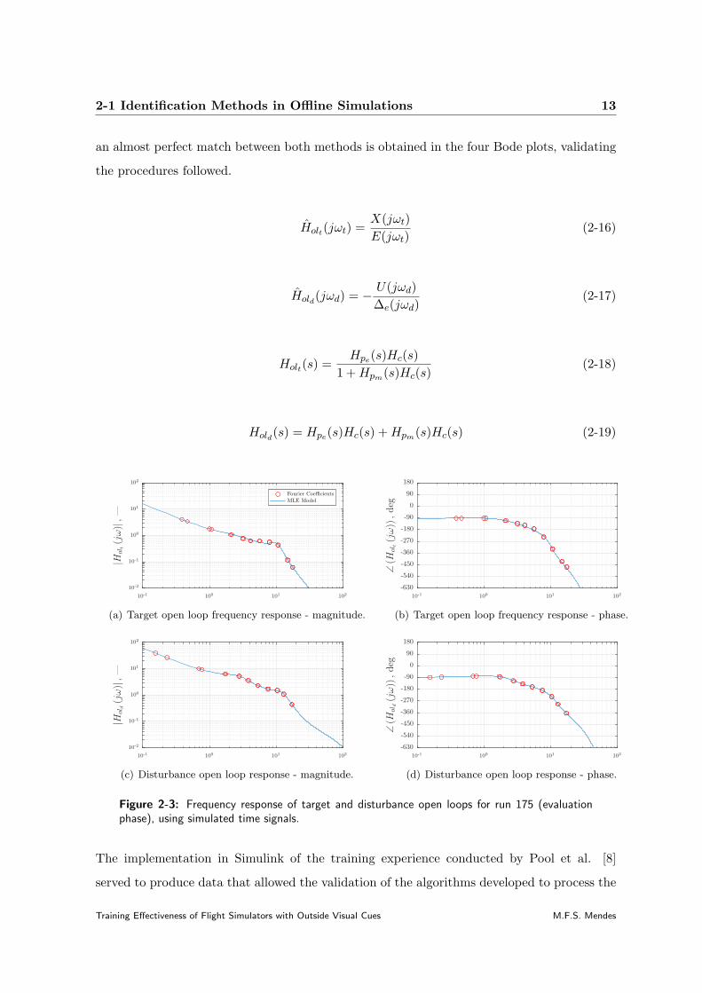
In Figure 2-3 the frequency response of target and disturbance open loops is shown, calculated

using the Fourier coefficients of the signals that define respectively the target and disturbance

open loops, as given in Eqs. (2-16) and (2-17) (where ∆e represents the Fourier Transform of

the time signal corresponding to the elevator command, δe), and recurring to the parameters

determined by the MLE identification algorithm, according to Eqs. (2-18) and (2-19). Again,



an almost perfect match between both methods is obtained in the four Bode plots, validating

the procedures followed.

Holt(jωt) =X(jωt)

E(jωt)(2-16)

Hold(jωd) = −U(jωd)

∆e(jωd)(2-17)

Holt(s) =Hpe(s)Hc(s)

1 +Hpm(s)Hc(s)(2-18)

Hold(s) = Hpe(s)Hc(s) +Hpm(s)Hc(s) (2-19)

Fourier Coefficients

MLE Model

|Hol

t(jω)|,—

10-1 100 101 10210-2

10-1

100

101

102

(a) Target open loop frequency response - magnitude.

∠(H

olt(jω)),deg

10-1 100 101 102-630

-540

-450

-360

-270

-180

-90

0

90

180

(b) Target open loop frequency response - phase.

|Hol

d(jω)|,—

10-1 100 101 10210-2

10-1

100

101

102

(c) Disturbance open loop response - magnitude.

∠(H

old(jω)),deg

10-1 100 101 102-630

-540

-450

-360

-270

-180

-90

0

90

180

(d) Disturbance open loop response - phase.

Figure 2-3: Frequency response of target and disturbance open loops for run 175 (evaluationphase), using simulated time signals.

The implementation in Simulink of the training experience conducted by Pool et al. [8]

served to produce data that allowed the validation of the algorithms developed to process the



results of the current experiment. In this Section, the main results of identification techniques

were shown, but during the experiment preparation the results gathered with this simulation

were also useful to develop and validate other algorithms and analysis techniques typically

used in tracking experiments, like coherence determination, crossover frequency, and phase

margin estimation, decomposition of tracking error and control activity variance, and other

dependent metrics used to evaluate the results of the current experiment.


2-2 Pilot Experiments 15

2-2 Pilot Experiments

Following the literature study developed and the offline simulations, the design of the training

experiment began. In this section, insight on crucial aspects of the experiment design is given,

justifying the most relevant design decisions made. Namely, two pilot experiments to define

the final controlled element dynamics and the outside visual scene are described and their

results analyzed.

2-2-1 Controlled Element Dynamics

The first design choice to be made for the final experiment was the dynamics to be controlled.

A pilot experiment was conducted in the SRS on March 9, 2016, where three different dy-

namics were tested, and the results processed to evaluate how these dynamics performed in

terms of controlling effort, tracking performance and human operator modeling. The task

performed is shown in Fig. 2-4. Human operators perceived the tracking error to minimize

with a compensatory display presented in the Primary Flight Display (PFD), shown in Fig.

2-5. No other cues were provided (the SRS outside visual and motion systems were off).

Human Operator

ft +

-

e

Error Response

Hpe

ue

n

+ + u

fd

++Controlled Dynamics

Hcφδ

Figure 2-4: Schematic representation of the roll tracking task.

Figure 2-5: Compensatory tracking display shown in the PFD.



The dynamics tested are described in the following paragraphs, together with a description

of the structure of the human operator control behavior model utilized. In Fig. 2-6 the

frequency response of the three dynamics tested is shown.

1. The first dynamics tested were the dynamics used in the training experiment mentioned

in Sec. 2-1. The dynamics are given in Eq. (2-1) and correspond to a reduced-order

linearized model for the elevator-to-pitch dynamics of a Cessna Citation I.

Considering the frequency response shown in Fig. 2-6, the structure for the human

operator behavior was chosen the same as the one introduced in Sec. 2-1, with the error

response model given by Eq. (2-20), being equivalent to the one used in Pool et al. [8].

This structure is chosen for the human operator model following the crossover model by

McRuer et. al (1965) [21], making the dynamics of the target open loop in the crossover

region to approximate a single integrator.

Hpe(s) = Ke(Tleads+ 1)2

Tlags+ 1e−sτeHnm(s) (2-20)

With Hnm(s) representing the neuromuscular system dynamics given in Eq. (3-4).

Hnm(s) =ω2nm

s2 + 2ζnmωnms+ ω2nm

(2-21)

Six parameters define the human operator equalization response: the error gain Ke, a

lead time constant, Tlead, and a lag time constant, Tlag. Human operator limitations

are included in a time delay τe and in the neuromuscular system, a second-order system

characterized by a natural frequency ωnm and a damping ratio ζnm.

2. The second dynamics tested correspond to the dynamics used by P. M. T. Zaal et al.

[16], from a mid-size twin-engine commercial transport aircraft with a gross weight of

185,800 lbs. The roll dynamics, given in Eq. (2-22), correspond to a linearization close

to the stall point, at an altitude of 41,000 ft and an airspeed of 150 kts.

Hc(s) = 3.91040

(

s2 + 0.2175s+ 0.5861)

(s+ 0.7599) (s− 0.02004) (s2 + 0.1133s+ 0.6375)(2-22)



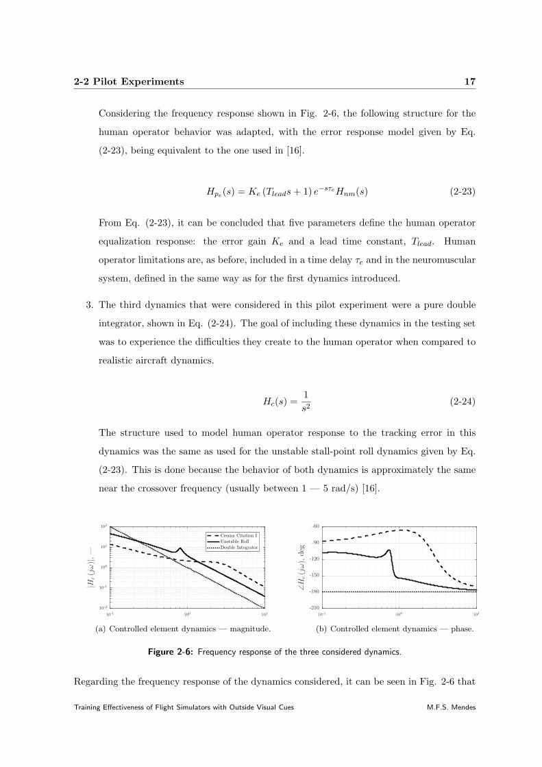
Considering the frequency response shown in Fig. 2-6, the following structure for the

human operator behavior was adapted, with the error response model given by Eq.

(2-23), being equivalent to the one used in [16].

Hpe(s) = Ke (Tleads+ 1) e−sτeHnm(s) (2-23)

From Eq. (2-23), it can be concluded that five parameters define the human operator

equalization response: the error gain Ke and a lead time constant, Tlead. Human

operator limitations are, as before, included in a time delay τe and in the neuromuscular

system, defined in the same way as for the first dynamics introduced.

3. The third dynamics that were considered in this pilot experiment were a pure double

integrator, shown in Eq. (2-24). The goal of including these dynamics in the testing set

was to experience the difficulties they create to the human operator when compared to

realistic aircraft dynamics.

Hc(s) =1

s2(2-24)

The structure used to model human operator response to the tracking error in this

dynamics was the same as used for the unstable stall-point roll dynamics given by Eq.

(2-23). This is done because the behavior of both dynamics is approximately the same

near the crossover frequency (usually between 1 — 5 rad/s) [16].

Cessna Citation IUnstable RollDouble Integrator

|Hc(jω)|,—

10-1 100 10110-2

10-1

100

101

102

(a) Controlled element dynamics — magnitude.

∠H

c(jω),deg

10-1 100 101-210

-180

-150

-120

-90

-60

(b) Controlled element dynamics — phase.

Figure 2-6: Frequency response of the three considered dynamics.

Regarding the frequency response of the dynamics considered, it can be seen in Fig. 2-6 that



both the pitch and the unstable dynamics approach the double integrator dynamics for high

frequencies. On low frequencies, the unstable dynamics and the pitch dynamics are similar to

a single integrator, which means they will be easier to control than the double integrator. The

main difference in terms of frequency response between these two dynamics is the crossover

frequency, which is higher for the Cessna Citation I, and the phase, which is higher for the

pitch dynamics and therefore further away from the critical -180 degrees at the crossover

frequency. These two effects combined make the pitch dynamics easier to control than the

unstable dynamics.

Results

Two testing subjects performed three tracking runs with each of the previous defined dynam-

ics. The runs were averaged to mitigate measurement noise and non-linearities affecting the

runs. One subject, henceforth mentioned as subject 1, had significant experience in compen-

satory tasks and the other subject, henceforth mentioned as subject 2, had relatively little

experience in tracking tasks. The dynamics are henceforth referred to as P, U and D, mean-

ing, respectively, the Cessna Citation I elevator-to-pitch dynamics of Eq. (2-1), the unstable

stall-point roll dynamics of Eq. (2-22) and the pure double integrator dynamics of Eq. (2-24).

Tracking Error and Control Activity RMS

In Figure 2-7 the average of the root mean square value of the tracking error and control

activity time signals of the three runs performed in each condition is shown for both subjects.

It is visible the differences in task proficiency of the subjects. Both subjects performed better

with the Pitch dynamics, and the double integrator yielded the worse results. The unstable

dynamics constitute an intermediate situation between the other two considered dynamics.

Human Modeling Parameters

A time-domain identification algorithm was applied to the three-run average for each condi-

tion. The method, described in [20], consists on a genetic algorithm optimization method to

generate the initial estimation of a Gauss-Newton optimization procedure. The results ob-

tained for each subject are shown in Table 2-2. It can be seen that Subject 1 has higher gains



Subject 1Subject 2

Dynamics

σe,deg

P U D

0

1

2

3

4

(a) Tracking error.Dynamics

σu,deg

P U D

0

1

2

3

4

(b) Control input.

Figure 2-7: Root mean square value of tracking error and control activity for both subjects inthe three dynamics tested.

in every dynamics, together with lower lead constants and higher lag constants, which is con-

sistent to what was found in terms of tracking performance. Subject 1 has approximately the

same neuromuscular frequency and damping ratio in every dynamics, while subject 2 shows

more variation, especially in the double integrator case. For these dynamics, the damping

coefficient is higher than 1 suggesting the model did not hold a proper estimation of this

neuromuscular parameter.

Table 2-2: Parameter estimates for both subjects for three dynamics tested.

Pitch Dynamics Unstable Dynamics Double Integrator

Ke, — Tlead, s Tlag, s τe, s ωnm, rad/s ζnm, — Ke, — Tlead, s τe, s ωnm, rad/s ζnm, — Ke, — Tlead, s τe, s ωnm, rad/s ζnm, —

Subject 1 3.76 0.52 1.53 0.23 10.41 0.23 1.04 0.63 0.24 10.59 0.15 0.61 0.83 0.22 10.32 0.17Subject 2 2.21 0.78 2.60 0.27 9.42 0.65 0.39 1.15 0.28 9.26 0.62 0.14 2.23 0.37 19.87 1.08

In Figures 2-8 and 2-9, the frequency response of the identified human control behavior and

the target open loop are, respectively, shown for subject 1. Considering these plots, it can be

seen again that the unstable roll dynamics are an intermediate situation between the other

two dynamics. Pilot behavior in pitch and unstable dynamics is similar, and in the open

loop it is visible that, while the crossover frequency is approximately the same, the unstable

dynamics have a lower phase margin than the pitch dynamics.

In Fig. 2-10, where crossover frequencies and phase margins are shown for both subjects, it

can be seen that on one hand the phase margin of the double integrator is small, indicating

difficulties for the human operator to successfully control the system, and on the other hand

the pitch dynamics make the task relatively easy. It can also be seen that subject 2 has a




ω, rad/s

|Hpe(jω)|,—

10-1 100 101 10210-1

100

101

(a) Human operator response — magnitude.

ω, rad/s

∠(H

pe(jω)),deg

10-1 100 101-500

-400

-300

-200

-100

0

100

(b) Human operator response — phase.

Figure 2-8: Subject 1 frequency response for the three dynamics tested.


ω, rad/s

∣ ∣

Hpφ(jω)∣ ∣,—

10-1 100 101 10210-2

10-1

100

101

102

(a) Open loop frequency response — magnitude.

ω, rad/s

∠(

Hpφ(jω))

,deg

10-1 100 101 102-600

-500

-400

-300

-200

-100

0

(b) Open loop frequency response — phase.

Figure 2-9: Subject 1 target open loop frequency response for the three dynamics tested.

Subject 1

Subject 2

Dynamics

ωc,rad/s

P U D

0

1

2

3

4

(a) Disturbance open loop crossover frequency.Dynamics

φm,deg

P U D

20

40

60

80

100

(b) Target open loop phase margin.

Figure 2-10: Target open loop crossover frequency and phase margin for both subjects for thethree dynamics tested.



abnormally high phase margin for the pitch dynamics, but his crossover frequency is, con-

trastingly, abnormally low, being a good example on the trade-off a human operator has to

make on a tracking task between performance and stability.

Conclusions

Regarding the pilot experiment made to decide which dynamics would be used on the fi-

nal experiment setup, the following conclusions were drawn based on the results previously

presented and on the opinion of both subjects performing the pilot experiment.

• Pitch Dynamics: These dynamics are easy to control, even for task-naive partici-

pants, which means that it is unlikely that task-naive subjects loose the control of these

dynamics. This is a clear advantage of these dynamics because if that would happen

the training progress would be interrupted, and furthermore if it would happen on a

motion-base condition it would cause a simulator crash, which is something to avoid.

Furthermore, there is also background research available where these dynamics were

used, which allows for a cross-checking of the final results. However, these dynamics

might be excessively easy, failing to challenge subjects who need to perform 200 tracking

runs. Also, with easy dynamics, subjects might master them on a early stage of the

experiment, jeopardizing the exponential acquisition of manual control skills expected;

• Unstable Roll Dynamics: These dynamics, while being harder to control than the

previous ones, are also relatively easy to master, which makes it again unlikely for

subjects to loose control over these dynamics. Being slightly harder makes these dy-

namics more suitable to performance improvements throughout the 200 tracking runs

performed by each subject. The most considerable difference between these dynamics

and the pitch dynamics is the constant focus necessary to execute the control tracking

task with these dynamics, given their unstable characteristic. Background research done

with these dynamics also provides a safety net for cross-checking final results, however

not in the same degree as the previous dynamics do, with whom training experiments

with task-naive subjects have already been performed;

• Double Integrator Dynamics: Given the marginal stability of the double integrator,

these are the hardest dynamics to control. They require a permanent focus of the



participant, which is an advantage as participants would need to be extremely focused

throughout the entire experiment, but it can also increase fatigue effects on the subjects.

However, given the naivety of the subjects who will be performing the experiment, these

dynamics might cause problems in motion conditions where simulator limits are easily

attained.

Given the aforementioned arguments, which were carefully weighted and evaluated, the final

decision was to utilize in this training experiment the unstable dynamics given in Eq. (2-22),

as they offer a piece of both worlds, being challenging enough without being excessively hard

to control.

2-2-2 Outside Visual Cues

The second main choice to be made regarding the final experiment setup was the outside

scenario to provide out-of-the-window visual cues to the human operator. Again, three options

were considered for the outside visual scene and a pilot experiment was performed on the

SRS to evaluate what outside visual scenario best fitted the experiment purpose. This pilot

experiment was performed on April 28, 2016, and consisted on a tracking task similar to the

one described in the previous section, with the addition of a feedback path to the controlled

dynamics, which could be provided by motion and/or visual cues, defining four conditions

(C1, C2, C3 and C4) as explained in Table 2-3, with the tracking error being presented in

the PFD in the form of a compensatory display for every condition.

Table 2-3: Experimental conditions for the outside visual cues pilot experiment.

PFD Outside Visuals Motion

C1 On Off OffC2 On On OffC3 On Off OnC4 On On On

The dynamics utilized were the ones chosen in Section 2-2-1, the unstable stall-point roll

dynamics given in Eq. (2-22). The tracking task block diagram is given in Fig. 2-11, where

the dashed channel represents the roll response which is available when motion and/or visual

cues were provided, meaning that in C1 only the error response channel is considered in



the human operator model. Therefore in this pilot experiment a double-channel structure

was considered for conditions C2, C3 and C4, where the error response was modeled in the

same way as in the previous pilot experiment (Eq. (2-23)), and the response to the roll

feedback (provided by the outside visual scene and/or the physical motion of the simulator)

was modeled with the structure given in Eq. (2-25).

Hpφ(s) = sKφe−τφsHnm(s) (2-25)

Human Operator

ft +

-

e

Error Response

Hpe

Roll Response

Hpφφ

ue

n

uφ

-

+ + u

fd


Hcφδ


A description of the three scenarios considered is given in the following paragraphs.

• Vertically moving checkerboard patterns: This outside visual scenario provides

peripheral visual cues using two vertically moving checkerboards positioned in the lateral

windows of the simulator’s cockpit. The checkerboards move vertically according to the

roll angle, providing human operators with roll rate information without giving a roll

angle reference. While being a peripheral visual cue and not a fully outside visual cue,

the checkerboards are reported to give strong roll inputs, as peripheral visual cues are

known to be primarily important in visual motion perception [22], and were already

used in roll compensatory tracking tasks [13]. In Fig. 2-12(a) one checkerboard panel

is displayed, and in Fig. 2-12(b) the visual on the simulator cockpit is shown.

• Realistic outside environment: This outside visual scenario consists on a realistic

environment corresponding to Schiphol Airport, in Amsterdam, the Netherlands. The

center projection of the visual scene presented to the human operator is shown in Fig.



(a) Right checkerboard. (b) Simulator cockpit.

Figure 2-12: Checkerboard visual scene.

2-13(a), with the simulator cockpit in 2-13(b). When considering a realistic outside

environment to provide roll cues, some aspects were taken into account. If a realistic

situation is adopted, with the simulated aircraft flying at a certain altitude, then the

horizon line is barely visible from the pilots’ position, thus resulting in poor roll rate

feedback information and in a weak roll sensation when motion is not provided. To

increase the available visual information, elements like clouds could be added to the

visual scenario, or the altitude could be lowered, so that the horizon line, buildings, trees

and other elements of Earth surface are visible to the pilot, providing the needed roll

information. The last solution was adopted, thus the outside environment presented to

human operators consisted on a fixed 5 meter height perspective, that will roll following

the controlled element dynamics. The reduced height causes a perception of the roll

rotation based on the position of the horizon line and its relative position with respect

to the buildings and other visible elements.

• Flow-field environment: This outside visual scenario gives information on the dy-

namics exploring flow-field perception. It consists on a black background with white

dots randomly distributed in a simulated 3-dimensional space, projected in the windows

of the simulator cockpit as shown in 2-14(b) and simulates a star field, shown in Fig.

2-14(a). This scenario is based on the optic flow concept. When the simulation starts,

a radial optic flow pattern emerges, created by the stars through two types of simulta-

neous movement, a translational and a rotational movement, made with respect to the

central point of the projected image, the focus of radial outflow [23]. To understand how



(a) Realistic visual scene. (b) Simulator cockpit.

Figure 2-13: Realistic visual scene.

(a) Flow-field scene. (b) Simulator cockpit.

Figure 2-14: Flow-field visual scene.

the projection is generated, it helps if the human operator moving through the world

is modeled using a camera analogy. The translational movement is simulated with a

constant forward speed of the camera, and the rotational movement is simulated with

the rotation of the camera around an axis perpendicular to the perspective according

to the roll angle of the controlled element. The combination of both aspects provides

a strong visual perception of the controlled dynamics. To the described visual scenario

a explicit compensatory display showing the tracking error was added, overlapped in

the visual scenario, repeating the information provided in the PFD. This was done so

that a reference for the null error was explicitly given, because if the null position is

only provided by the PFD then this visual cue would become peripheral (the human

operator would have to look down to perform the task).



Results

The same two test subjects who performed the dynamics pilot experiment performed the

task in the four conditions for the three outside visual scenes, making a total of 12 runs per

subject. The results are subsequently described.

Tracking Error and Control Activity RMS

In Figure 2-15, the RMS of the tracking error and the control input are shown for both

subjects, in the four cues combinations and the three outside scenarios. The difference in

performance of both subjects is again clear as all the red lines in Fig. 2-15(a) are above the

blue lines. To compare visual scenarios, conditions 2 and 4 should be considered, because

in these conditions the outside visuals are On. For Subject 1, the best performances are

attained with the checkerboards and the worse with the flow-field. For Subject 2 the best

performances are attained with the realistic environment, while the checkerboards and the

flow-field register similar performances.

Subject 1Subject 2CheckerboardsRealisticFlow Field

σe,deg

C1 C2 C3 C4

0

1

2

3

4

(a) Tracking error RMS.

σu,deg

C1 C2 C3 C4

0

1

2

3

4

5

(b) Control input RMS.

Figure 2-15: RMS of signals e and u for both subjects in the three outside visuals tested.

Human Operator Modeling Results

The 24 runs performed were submitted to a maximum likelihood time domain identification

procedure in order to estimate the parameters defining the error response Hpe and the roll

response Hpφ of the human operator. Each run was individually identified, thus without

performing any between-runs averaging, degrading the quality of the estimates. The results



of the human operator control behavior in condition 2 (with the outside visual scene on and

the physical motion cues off) will be carefully analyzed, because in this condition outside

visual cues are mostly relevant to the creation of the roll feedback channel.

In Fig. 2-16, Subject 1 error and roll frequency response plots are shown, for the three outside

visuals provided, in condition C2. Given that only outside visual cues were provided in C2,

they are exclusively responsible for the creation of the roll response. It is visible in Fig.

2-16(c) that the checkerboards provide the strongest roll feedback channel. The flow-field

fails to create effectively this feedback channel. If open loop frequency response is considered,

shown in Figure 2-17, it is clear that with the checkerboards this human operator registered

the best open-loop characteristics, and therefore with the checkerboards the roll feedback

channel is the most effective from the three tested visuals.

CheckerboardsRealisticFlow Field

ω, rad/s

|Hpe(jω)|,—

10-1 100 101 10210-2

10-1

100

101

102


ω, rad/s

∠(H

pe(jω)),deg

10-1 100 101 102-630

-540

-450

-360

-270

-180

-90

0

90

180


ω, rad/s

∣ ∣

Hpφ(jω)∣ ∣,—

10-1 100 101 10210-2

10-1

100

101

102

(c) Roll response - magnitude.

ω, rad/s

∠(

Hpφ(jω))

,deg

10-1 100 101 102-630

-540

-450

-360

-270

-180

-90

0

90

180

(d) Roll response - phase.

Figure 2-16: Frequency response of Subject 1 for C2 (Visuals On, Motion Off), comparing thethree outside visual scenarios.

Crossover Frequencies and Phase Margins

In Figure 2-18 the disturbance and target crossover frequencies and phase margins for both

subjects are shown. Looking at C2 from subject 1, it is seen that checkerboards cause a



CheckerboardsRealisticFlow Field

replacemen

ω, rad/s

|Hol

d(jω)|,—

10-1 100 101 10210-2

10-1

100

101

102

(a) Disturbance open loop - magnitude.

ω, rad/s

∠(H

old(jω)),deg

10-1 100 101 102-630

-540

-450

-360

-270

-180

-90

0

(b) Disturbance open loop - phase.

ω, rad/s

|Hol

t(jω)|,—

10-1 100 101 10210-2

10-1

100

101

102

(c) Target open loop - magnitude.

ω, rad/s

∠(H

olt(jω)),deg

10-1 100 101 102-630

-540

-450

-360

-270

-180

-90

0

(d) Target open loop - phase.

Figure 2-17: Open loop frequency response of Subject 1 for C2 (Visuals On, Motion Off),comparing the three outside visual scenarios.

better performance (higher crossover frequencies and lower phase margins). For subject 2,

the same is visible in target crossover frequency and both phase margins, while no clear

difference between the scenarios exists in disturbance crossover frequency. In C2 and for both

subjects, the flow-field visual scenario yields the worse results in these parameters, with the

realistic environment yielding intermediate results. Furthermore, motion is seen to decrease

target crossover frequencies and increase disturbance crossover frequencies and target phase

margins. No clear effect on disturbance phase margin is seen to be introduced by motion.

Conclusions

Considering the pilot experiment designed to decide which outside visual scene would be uti-

lized as out-of-the-window visual cue in this training experiment, the following considerations

were drawn based on the results presented in this Section and on the opinion of both subjects

performing the test session.



wc d,rad/s

C1 C2 C3 C4

0

1

2

3

4

(a) Disturbance crossover frequency.

Subject 1Subject 2CheckerboardsRealisticFlow Field

φd,deg

C1 C2 C3 C4

0

25

50

75

100

(b) Disturbance phase margin.

wc t,rad/s

C1 C2 C3 C4

0

1

2

3

4

(c) Target crossover frequency.

φt,deg

C1 C2 C3 C4

0

25

50

75

100

(d) Target phase margin.

Figure 2-18: Crossover frequencies and phase margins for both subjects in the three outsidevisual scenes tested.

• Vertically moving checkerboard patterns: This out-of-the-window visual cue has

the main advantage of providing a strong visual roll rotation input with relative sim-

plicity. Another advantage is the fact that it was already used in previous roll-tracking

tasks, with its effects being well-known and described. It is not however a full out-of-the-

window visual cue, as it provides only peripheral visual cues. This fact is nonetheless

not problematic because it is known that peripheral visual cues are the main responsi-

ble for the visual perception of motion, and subjects performing tracking experiments

with these visuals reported that checkerboards made them feel like if they were actually

moving.[13] This translated to the results obtained in this test session, with the verti-

cally moving checkerboards proving to be clearly more effective in giving roll motion

feedback than the other visual cues. This is visible in lower tracking error RMS, higher

gains in the roll feedback response and higher crossover frequencies attained with the

checkerboards as visual cue. The fact that this cue is not realistic may constitute a

disadvantage in terms of transferring the results of the experiment to real flight sim-

ulators, but on one hand the entire experiment has a fundamental character typical



in academic research, and on the other hand, the remaining solutions do not offer a

significant increase in terms of realism. Another positive point of these dynamics is the

fact that they are highly unlikely to create motion sickness.

• Realistic outside environment: This visual setup is the visual cue which is clos-

est to reality, but the fact that the aircraft was simulated to be in low altitude and

not moving forward lowers the realism of this scenario. Subjects also reported some

sickness effects caused by this visual scene. Looking at the results obtained when the

Schiphol Airport environment was given as roll cue, it was seen that these cues provide

a strong visual input, with good results in tracking performance and human operator

modeling results. Another effect described by the subjects was the fact that it was not

easy to steer the dynamics to the null error, which is explained by the fact that these

dynamics provide roll-attitude reference, as the zero error corresponds to the horizon

being aligned. Therefore subjects would try to minimize the error without looking at

the PFD, which leads to worse performance because perceiving zero error is easier with

the explicit compensatory display.

• Flow-field environment: This out-of-the-window visual cue was the less effective in

providing a strong roll rotation perception, registering the worse tracking performances,

an effect also seen in human operator modeling results. Subjects described some motion

sickness caused by the flow-field environment. They also reported that the perception

of the zero-error position was harder with this cue, because they would not look at the

explicit display in the PFD but to the explicit display which was overlapped into the

visuals, where it was harder to perceive the null position, possibly due to the interaction

with the visual background. This scene was developed to take advantage of optic flow

concepts, which were previously applied to tracking tasks but not in a roll-axis tracking

task. The results of this test session seem to prove that this concept fails to be effective

as a roll cue, but a more extensive study, with perhaps a different concretization of the

optic flow concept, would be beneficial to further validate this conclusion.

Considering the results presented, together with the opinions collected from the subjects and

the arguments described, the conclusion of this test session was to use the checkerboards as

the outside visual cue in this quasi-transfer-of-training experiment.


Chapter 3

Experimental Methods

Following the experiment design decisions given in the previous Chapter, the methods followed

and the full experiment design are given in this Chapter, with a description of the control

task, the experiment setup, the participants and the apparatus, followed by a description on

the way the experimental data was analyzed. This Chapter ends with the main hypothesis

to be tested.

3-1 Control Task

This human-in-the-loop training experiment considered a compensatory roll-axis tracking

task, following the same procedures as various earlier investigations on skill-based manual

control training [8, 15, 16, 13]. In Figure 3-1 this task is schematically represented. The

human controller was asked to follow a target roll angle, specified by the tracking signal ft,

as accurately as possible. Simultaneously, the human operator had to reject disturbances on

the controlled system Hc, which were induced by the disturbance signal fd. This disturbance

signal was summed to the human operator’s input, u, and directly affected the controlled

dynamics. In order to identify and model the multi-channel human operator response, char-

acterized by Hpe and Hpφ , the disturbance signal fd and the target signal fd were independent


32 Experimental Methods

sum-of-sines signals [24, 19, 20]. Given the quasi-linear human operator model used, the con-

trol input had contributions from the error response, ue, the roll response, uφ, and a remnant

n accounting for nonlinear behavior and measurement noise.

Human Operator

ft +

-

e

Error Response

Hpe

Roll Response

Hpφφ

ue

n

uφ

-

+ + u

fd


Hcφδ


In the experiment (see Fig. 3-2(a)), the human operator perceived the dynamics being con-

trolled with a compensatory display which resembled a basic Primary Flight Display (PFD),

shown in Fig. 3-2(b). This compensatory display showed the deviation e between the current

aircraft roll angle, φ, and the target roll angle, ft.

The out-of-the-window visual cues used were chosen with a pilot experiment described in

Section 2-2-2 and are based on various compensatory roll-axis tracking experiments [25, 1,

26, 13]. They consisted on two vertically moving checkerboard panels (see Fig. 3-2(c)),

providing a strong roll motion sensation without giving reference of roll-attitude. In the

moving base condition pure roll motion was provided, thus without any washout or lateral

specific force compensation.

(a) Simulator Cockpit.

e

(b) Central Display. (c) Out-of-the-window visuals.

Figure 3-2: Simulator cockpit, central display and the out-of-the-window scene.

The controlled dynamics Hc were also chosen with a pilot experiment, described in 2-2-1.


3-1 Control Task 33

ω, rad/s

|Hc(jω)|,—

10-1 100 10110-2

10-1

100

101

102

ω, rad/s

∠H

c(jω),

deg

10-1 100 101-180

-150

-120

-90

Figure 3-3: Frequency response of the controlled element dynamics.

They are the dynamics used in Ref. [16] presented in Eq. (3-1), multiplied by a gain of

5. These dynamics correspond to a mid-size twin-engine commercial transport aircraft with

a gross weight of 185,800 lbs, linearized in a flight condition close to the stall point, at an

altitude of 41,000 ft and an airspeed of 150 kts.

Hc(s) = 3.91040

(

s2 + 0.2175s+ 0.5861)

(s+ 0.7599) (s− 0.02004) (s2 + 0.1133s+ 0.6375)(3-1)

An obvious remark regarding the transfer function presented in Eq. (3-1) is that the roll

dynamics of the aircraft are unstable, due to the spiral mode. These dynamics approximate

a single integrator(

1s

)

at low frequencies (< 0.75 rad/s) and a double integrator(

1s2

)

at

frequencies higher than 0.75 rad/s, as seen in Fig. 3-3, due to the effect of the pole at

s = -0.7599 rad/s.

The human operator control behavior was modeled in this compensatory tracking task using

a quasi-linear model [21, 27]. As shown in Fig. 3-1, the output of the human operator, the

control input signal u, is the sum of a linear response and a remnant signal n. The linear

response has two contributions, Hpe and Hpφ , which respectively model the response to the

roll tracking error (available from the PFD) and the response to the roll feedback (available

via the out-of-the-window cues or simulator’s motion) [28, 29]. The remnant signal accounts

for measurement noise and nonlinearities which are not described by the linear response

functions. Determining the form of the transfer functions Hpe and Hpφ and the evolution of

their parameters throughout the progress of a training experiment has proven to be of great

help in understanding and quantifying the learning process of both visual and motion cues

by the initially task-naive participants [16, 30].



3-2 Forcing Functions

The disturbance and target forcing functions, fd and ft, were independent sum-of-sines signals

defined by Eq. (3-2), as used in a number of previous tracking studies [19, 24, 31].

fd,t(t) =

Nd,t∑

k=1

Ad,t[k] sin (ωd,t[k]t+ φd,t[k]) (3-2)

In Eq. (3-2), Ad,t[k], ωd,t[k] and φd,t(k) respectively indicate the amplitude, frequency and

phase of the k-th sine in the forcing function. Nd,t is the number of sine waves constituting

the forcing function. In this experiment, both the disturbance and target forcing functions

were the sum of Nd,t = 20 individual sinusoids, each with different amplitudes, frequencies

and phases. In Table 3-1 a list of all the parameters used to generate the forcing functions

can be found.

The frequencies of the sinusoids, ωd,t[k], were purposely defined as integer multiples of the

measurement time base frequency, ωd,t[k] = nd,t[k] ωm, where ωm = 2π/Tm = 0.0767 rad/s

and Tm = 213/fs = 81.92 s is the measurement time, counting from the end of the run (each

run had 95 seconds and only the last 81.92 seconds were used, using a sampling frequency of

fs=100 Hz). The selected integer multiples were used in previous studies [8], guaranteeing

the twenty sinusoid frequencies covered the frequency range of human control at regular

intervals on a logarithmic scale. Moreover, the integer multiples were chosen in consecutive

pairs, creating double bands of input frequencies so that coherence between the control signal

produced by the human operator u and the forcing functions fd and ft could be calculated,

which allowed the evaluation of human control linearity in each individual run [32].

A second-order low-pass filter was used to calculate the amplitudes of the individual sines, in

similarity with previous studies [8, 31]. The purpose of this second-order filter was to reduce

the magnitude of the amplitudes at higher frequencies, which results in a not extremely

difficult tracking task. Also matching earlier experiments [8, 31], the amplitude distributions

were scaled so that the target forcing function power was 25% of that of the disturbance

forcing function, which made this task predominantly a disturbance-rejection task.

Five realizations of fd and ft were used, differing only by their initial sinusoidal phases φd,t of

the individual sine-components. The set of phases chosen yielded signals with a Gaussian-like


3-3 Experiment Setup 35

Table 3-1: Experiment forcing function (disturbance and target) data

Disturbance signal, fd Target signal, ftnd ωd, rad/s Ad, deg φd,1, rad φd,2, rad φd,3, rad φd,4, rad φd,5, rad nt ωt, rad At, deg φt,1, rad φt,2, rad φt,3, rad φt,4, rad φt,5, rad2 0,15 0,03 6,28 3,52 2,64 2,83 2,96 5 0,38 0,51 5,68 3,99 3,92 6,00 4,393 0,23 0,05 1,25 5,41 2,07 5,64 1,00 6 0,46 0,49 0,83 4,35 1,42 5,23 5,779 0,69 0,13 1,46 2,16 5,64 5,18 4,57 13 1,00 0,34 0,54 5,35 5,17 4,75 4,9310 0,77 0,09 5,45 0,11 3,78 5,70 1,51 14 1,07 0,33 1,14 5,92 1,57 6,28 4,2322 1,69 0,27 1,96 0,66 4,94 4,09 1,81 27 2,07 0,16 2,93 3,84 4,05 2,88 4,0123 1,76 0,28 3,29 2,88 0,38 4,65 4,04 28 2,15 0,15 2,83 3,48 6,24 1,23 2,3936 2,76 0,36 2,62 1,96 1,88 4,43 3,33 41 3,14 0,08 6,02 4,99 4,04 1,21 2,9137 2,84 0,36 4,28 5,61 4,38 4,98 3,45 42 3,22 0,08 1,74 4,97 2,71 0,29 0,4649 3,76 0,40 6,28 5,63 0,73 3,80 4,31 53 4,07 0,06 3,90 4,26 1,71 1,88 2,5650 3,83 0,41 3,93 0,31 2,07 2,35 5,67 54 4,14 0,05 0,74 1,00 4,03 4,62 2,0869 5,29 0,47 4,39 0,65 4,09 3,60 1,54 73 5,60 0,03 5,65 4,69 0,67 0,89 4,5670 5,37 0,48 0,65 1,14 4,42 4,20 1,80 74 5,68 0,03 3,70 5,01 5,85 0,97 3,3397 7,44 0,59 6,17 0,35 2,82 0,34 6,24 103 7,90 0,02 3,63 5,44 5,13 0,74 1,4399 7,59 0,60 2,17 2,92 2,69 5,85 0,84 104 7,98 0,02 1,42 5,78 4,14 5,81 1,44135 10,35 0,79 3,80 2,27 4,91 4,54 3,25 139 10,66 0,02 3,64 0,86 2,66 5,21 5,97136 10,43 0,80 2,58 2,57 4,31 2,20 1,43 140 10,74 0,02 5,94 2,05 5,65 1,08 4,55169 12,96 1,03 2,84 6,07 4,46 6,16 4,57 193 14,80 0,01 4,74 2,03 4,28 0,70 5,76170 13,04 1,04 4,11 2,98 4,22 3,94 0,44 194 14,88 0,01 3,72 2,88 1,92 2,81 5,28224 17,18 1,53 4,98 0,77 4,69 2,20 3,57 229 17,56 0,01 4,32 3,01 1,03 4,44 2,67225 17,26 1,54 5,67 3,90 4,70 4,16 5,20 230 17,64 0,01 2,15 2,93 3,21 0,53 2,50

distribution and an average crest factor [33]. This was done in order to prevent subjects

from recognizing parts of the signals because of the repeated exposure inherent to performing

200 tracking runs. With a combination of five disturbance signals and five target signals,

randomly assigned to consecutive tracking runs following a latin-square distribution, it was

virtually impossible for the subjects to memorize the signals.

The disturbance signal was preshaped by the inverse of the aircraft dynamics to compensate

for the fact that it is actually inserted before Hc (see Fig. 3-1).

3-3 Experiment Setup

The experiment was divided in two phases, henceforth referred to as training and evaluation.

During the training phase, the task-naive participants were trained in the roll tracking task

previously described until their level of task performance stabilized. They were subsequently

transferred to the evaluation phase where the same roll tracking task was performed with

different cues being provided.

Participants were divided in two experimental groups, as shown in Fig. 3-4. The first group,

henceforth referred to as Group NV, was trained with only the PFD, thus without neither

out-of-the-window visuals or motion cues (NV NM), and they were transferred to evaluation

conditions where they had access to the PFD and motion feedback (NV M). The second

group, henceforth referred to as Group V, was trained without motion but with the PFD



and the out-of-the-window visual cues (V NM), and it was transferred to the same evaluation

configuration as the Group NV where the PFD and motion cues were available, without

peripheral visual cues (NV M). Therefore, the only difference between the two experimental

groups was the presence of out-of-the-window visual cues in the training phase.

Day 1

Session 1

25 runs

V NM

Session 2

25 runs

V NM

Day 2

Session 3

25 runs

V NM

Session 4

Transfer

25 runs

V NM

Day 3

Session 5

25 runs

NV M

Session 6

25 runs

NV M

Day 4

Session 7

25 runs

NV M

Session 8

25 runs

NV M

Visuals Group - Group V

Training Evaluation

Day 1

Session 1

25 runs

NV NM

Session 2

25 runs

NV NM

Day 2

Session 3

25 runs

NV NM

Session 4

Transfer

25 runs

NV NM

Day 3

Session 5

25 runs

NV M

Session 6

25 runs

NV M

Day 4

Session 7

25 runs

NV M

Session 8

25 runs

NV M

No - Visuals Group - Group NV

Training Evaluation

Figure 3-4: Quasi-transfer-of-training experiment design.

Each phase of the experiment consisted of a fixed number of 100 tracking runs, therefore each

subject performed 200 runs in total. The 95-second runs were performed in eight sessions of 25

runs each. The eight sessions were performed in four consecutive days, therefore two sessions

on each day, with a 20 minutes break between sessions (subjects left the simulator between

sessions). This experimental configuration allowed convergence of manual control skills in

both experimental phases, with a consolidation of the acquired control skills in between days

happening outside the simulator, an effect known as offline learning [34], and it also respected

the optimum retention time between training sessions of 24 hours [35].

The experiment was performed during five weeks on four consecutive working days of each

week. Two subjects performed their two daily sessions in the morning and two subjects

performed their two daily sessions in the afternoon, meaning a total of four subjects performed

the experiment in each week. To guarantee the balancing between subjects in the groups,

every subject in one week was placed in the same group. Therefore, two weeks had subjects

from Group NV, two weeks had subjects from Group V, and the fifth week had subjects from

both groups.

In the end of each tracking run, the researcher informed the subject of their score in that run


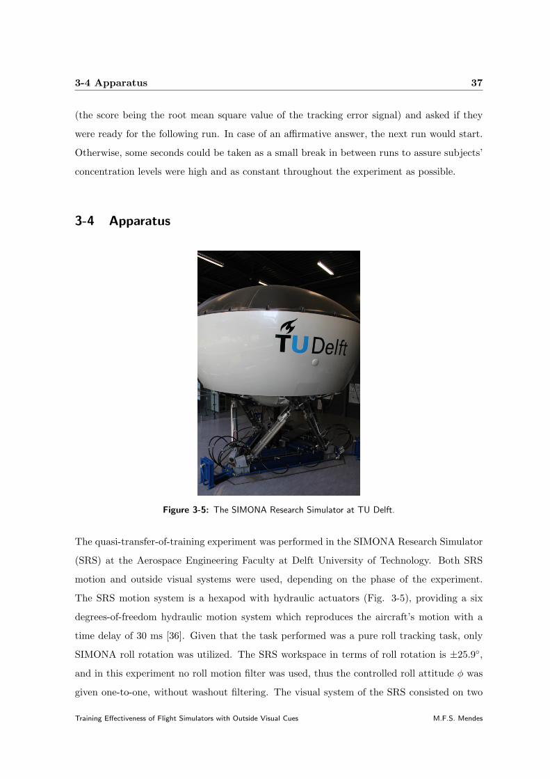
3-4 Apparatus 37

(the score being the root mean square value of the tracking error signal) and asked if they

were ready for the following run. In case of an affirmative answer, the next run would start.

Otherwise, some seconds could be taken as a small break in between runs to assure subjects’

concentration levels were high and as constant throughout the experiment as possible.

3-4 Apparatus

Figure 3-5: The SIMONA Research Simulator at TU Delft.

The quasi-transfer-of-training experiment was performed in the SIMONA Research Simulator

(SRS) at the Aerospace Engineering Faculty at Delft University of Technology. Both SRS

motion and outside visual systems were used, depending on the phase of the experiment.

The SRS motion system is a hexapod with hydraulic actuators (Fig. 3-5), providing a six

degrees-of-freedom hydraulic motion system which reproduces the aircraft’s motion with a

time delay of 30 ms [36]. Given that the task performed was a pure roll tracking task, only

SIMONA roll rotation was utilized. The SRS workspace in terms of roll rotation is ±25.9◦,

and in this experiment no roll motion filter was used, thus the controlled roll attitude φ was

given one-to-one, without washout filtering. The visual system of the SRS consisted on two



projectors generating the two checkerboard panels on the left and right window views of the

simulator cockpit. The visual system delay is approximately 30 ms and all displays were ran

at a 60 Hz refresh rate [37].

Participants sat in the simulator co-pilot seat and used a right-hand sidestick to control the roll

rotation of the aircraft. The pitch axis of the sidestick was locked so that only roll commands

could be given. The active stick was set to have a linear force-deflection characteristic of 0.75

N/deg without breakout-force. The simulator rolling motion was performed around an axis

aligned with the center of the right pilot seat to ensure pure roll cueing. The compensatory

display was located in front of the participant’s seat.

Each subject adjusted both the height of the seat and the distance of the seat to the sidestick to

ensure their comfort and the correct positioning of the checkerboards in their peripheral field

of vision. These seat settings were kept constant for each subject throughout the experiment.

Furthermore, participants used noise-canceling headphones with a masking aircraft engine

sound to fully hide the acoustic noise caused by the actuators of SRS motion system.

The SRS data recording system was set to work on a sampling frequency of 100 Hz, thus

yielding 9501 points of data per variable recorded for each tracking run.

3-5 Participants

To perform this training experiment, subjects could neither have any type of previous piloting

experience nor have participated in earlier tracking experiments. Another requirement the

subjects had to comply with was to be right-handed. An initial group of twenty fully task-

naive subjects, who gave their written consent to participate in this study, performed the

experiment. A total of ten subjects were included in each group, considering people between

18 and 23 years old, with nine different nationalities and three females (two placed in Group

NV and one in Group V). Two more subjects were tested in the experiment set, but due

to performance inconsistencies were omitted from the final data set. Each subject chose a

time slot (8 sessions of 1 hour each spread over four consecutive working days) and this

defined automatically the group in which they were inserted. Therefore no explicit selection

or distribution of the subjects between the experimental groups was made.


3-6 Data Analysis 39

3-6 Data Analysis

To understand how human operators acquire control skills throughout their learning process,

the data collected in the SRS was processed using a variety of mathematical tools and methods

which are carefully discussed in the following subsections.

3-6-1 Human Operator Modeling

Human operator control behavior was modeled and identified in each tracking run using a

multimodal quasi-linear operator model. Namely, the defining parameters of both the error

response transfer function Hpe and the roll feedback response transfer function Hpφ were

determined using identification and optimization algorithms. The models used for Hpe and

Hpφ were successfully used in earlier studies [12, 16, 31].

The considered model for the human operator error response Hpe is given by:

Hpe(s) = Ke (Tleads+ 1) e−τesHnm(s) (3-3)

With Hnm being the neuromuscular dynamics modeled by:

Hnm(s) =ω2nm

s2 + 2ζnmωnms+ ω2nm

(3-4)

For this roll tracking task with the considered controlled element dynamics, the error response

model included a gain Ke, a lead equalization term Tlead, a human operator response delay

τe, and the neuromuscular dynamics Hnm, modeled as a second-order mass-spring-damper

system with a neuromuscular frequency ωnm and a neuromuscular damping ratio ζnm. The

considered structure of Hpe is explained by the fact that human operators needed to generate

lead, because the controlled dynamics approximated a double integrator in the frequency

range where the human operator crossover frequency was expected to be for compensatory

tracking (1 - 5 rad/s) [16].

The human operator roll response Hpφ is modeled by:

Hpφ(s) = sKφe−τφsHnm(s) (3-5)



The roll response included a pure derivative term and an equalization gain Kφ, modeling

human operator limitations with a roll response delay τφ and the neuromuscular system,

modeled as in Hpe . It is convenient to mention that Hpφ characterized the sum of multiple

and separate feedback channels, namely the ones related with motion feedback, i.e., angular

accelerations detected by the semicircular canals, linear accelerations detected by the otoliths,

and motion cues from the somatosensory system [16]. For similar tasks, this model structure

has been successfully applied in earlier investigations [38]. The same human operator model

was used for experimental conditions in which either motion or out-of-the-window cues were

available. This allowed a direct assessment of how well out-of-the-window visual cues can

replace motion cues.

The multi-channel pilot model defined in Eqs. (3-3) to (3-5) contained seven free parame-

ters (Ke, Tlead, τe, Kφ, τφ, ωnm, and ζnm) which were estimated using maximum likelihood

time-domain parameter estimation techniques, as described in Section 2-1-3, on the collected

experimental data (the time-domain signals e, φ, and u). Obviously, in the training phase of

Group NV, only Hpe was fitted, as no out-of-the-window visual or motion cues were avail-

able. Firstly, ten repetitions of a genetic algorithm optimization were performed in order

to obtain ten initial rough estimates of the parameters, which were the starting point of a

Gauss-Newton optimization algorithm, yielding ten estimates for the set of parameters. The

estimate yielding the lowest value of the likelihood function was selected as the one describing

the control activity of the human operator in that run. If the lowest likelihood solution failed

to satisfy the physical restrictions inherent to the model (neuromuscular frequency between 0

and 30 rad/s and neuromuscular damping ratio between 0 and 1), another solution from the

set of ten Gauss-Newton estimates was considered. If none of the Gauss-Newton estimates

was in the domain of the model parameters, the genetic algorithm solution holding the lowest

likelihood was considered as the identified model of that run, with the validity of this lower

likelihood solution being carefully analyzed. Should this model describe the human operator

control behavior with an unacceptable low quality, the respective run would be omitted from

the final data set. This procedure was applied to the 200 runs in the training and evaluation

phases of each of the twenty subjects who performed the experiment, and from the set of 4000

tracking runs that compose the experiment, three were omitted from the final data set.

In every tracking run, the identified model Variance Accounted For (VAF) was calculated with


3-6 Data Analysis 41

Eq. (3-6) as a measure of the human operator model accuracy in describing the measured

control signal. The VAF is expressed in percentage and the higher the value, the better

the model describes what was exactly done by the human operator control behavior. It is

an usual practice in cybernetic studies to average the time signals over a certain number of

runs, to attenuate noise in the measured data and thus improving the model quality [31].

However, given the need to evaluate acquisition of control skills throughout individual runs,

averaging was not an option and therefore slightly lower VAF values were obtained due to

higher noise levels. Nevertheless, runs with abnormally low model VAFs (lower than 40 %)

were considered as identification outliers and excluded from the final data set considered, so

that they would not influence the group average results shown in Section III. A total of 56

runs were excluded from the final data set due to this reason, which is a reduced percentage

of excluded runs (1.4 %) for a training experiment with task-naive participants [8].

VAF =

(

1−

∑Ni=1 (u(t)− u(t))2∑N

i=1 u2(t)

)

× 100% (3-6)

The validity of the final model estimates was further analyzed with independently estimated

frequency-domain describing functions for Hpe and Hpφ , obtained with a black-box multiloop

identification method based on Fourier coefficients, as described in Section 2-1-2.

3-6-2 Other Dependent Variables

To further evaluate the progress of every subject and the effectiveness of training cues in the

evaluation setting, several additional dependent variables were calculated from the collected

data. Operator control activity and performance were evaluated, in the time domain, with the

variance of the control input, σ2u, and the roll tracking error, σ2

e , respectively, in accordance

to previous training studies [8, 16]. A decomposition on the sources (disturbance, target or

remnant) of these variances was also made. In the frequency domain, pilot performance in

rejecting the disturbance forcing function and following the target signal was determined by

the crossover frequencies and phase margins of the disturbance and target open-loop dynamics,

respectively [39]. The disturbance and target open-loop dynamics are given by (see Fig. 3-1):



Hol,d(s) = −u(s)

δ(s)=[

Hpe(s) +Hpφ(s)]

Hc(s) (3-7)

Hol,t(s) =φ(s)

E(s)=

Hpe(s)Hc(s)

1 +Hpφ(s)Hc(s)(3-8)

The disturbance and target crossover frequencies ωc,d and ωc,t are the frequencies where the

magnitude of the disturbance and target open-loop frequency responses is unity (0 dB). The

phase differences from -180 degrees at these crossover frequencies are the corresponding phase

margins φm,d and φm,t.

Finally, the coherence of the operators’ control input with respect to the disturbance and

target forcing signals was also estimated according to Eq. (3-9).

Γd,t (ωd,t [k]) =

√

√

√

√

√

∣

∣

∣Sfd,t (jωd,t [k])

∣

∣

∣

2

Sfd,tfd,t (jωd,t [k]) Suu (jωd,t [k])(3-9)

In Eq. (3-9), S (jωd,t [k]) represents the auto or cross power spectral density (PSD) function

of the signal. In each pair of averaged frequencies, ωd,t, the estimated coherence expresses

the linearity with respect to fd,t as a value between zero and one, where one means perfectly

linear control behavior [32].

3-6-3 Learning Curve Modeling

To give a quantitative insight on how operators’ control behavior changed during training

and after transfer to the evaluation condition, exponential learning curves were fitted to the

dependent measures described above. The learning curve model used is given by Eq. (3-10):

ylc(n) = pa + (1− F )n(p0 − pa) (3-10)

The exponential learning curve model in Eq. (3-10) is determined by the initial value p0, the

asymptotic value pa, and the learning rate F [6]. These parameters were calculated using

a non-linear optimization procedure using MatLab’s fminsearch to minimize the summed


3-7 Hypotheses 43

squared error between the experimental data yp and the learning curve model ylc, given in

Eq. (3-11). Each dependent variable had two learning curves associated, one for the training

phase and one for the evaluation. Pearson’s linear correlation coefficient ρ was determined to

evaluate fitness quality.

J =1

N

N∑

n=1

(yp(n)− ylc(n|p0, pa, F ))2 (3-11)

3-6-4 Statistical Analysis

A statistical analysis of the dependent data σ2e and σ2

u was performed to compare different

phases of the experiment. Three pairwise comparisons (dependent t-tests) were done for

each variable, corresponding to the expected evolutions throughout the experiment. Training

comparison took the average of each subject on runs 1-5 and 96-100. Transfer comparison

considered the average of each subject on runs 96-100 and 101-105. Evaluation comparison

contemplated the average of each subject on runs 101-105 and 196-200. The test utilized

in this statistical analysis was a nonparametric Wilcoxon signed-rank test, as the considered

data were mostly not normal distributed due to large between-subject differences.

3-7 Hypotheses

Based on a number of previous tracking experiments where the effects of both out-of-the-

window and motion cues were studied, together with earlier quasi-transfer-of-training studies,

the following hypotheses were formulated for this experiment:

H1: Training causes an improvement in performance and task proficiency in both experimen-

tal groups. Clear effects of training were expected to occur in both experimental groups during

the training phase, as seen in a number of previous training experiments (Refs. [7, 8, 16, 40]),

which are visible in improved performance (lower σ2e), increased control activity (higher σ2

u),

and higher crossover frequencies and phase margins. In the human operator modeling results,

it was expected to see adjustments in parameters that are known to be related to improved

performance (increased Ke, Kφ, lower human operator delays). Finally it was also expected



to see an increase on human operator linearity with training, measured with human operator’s

coherence.

H2: The presence of peripheral visual cues in training of control skills provides a feedback

channel of the controlled dynamics output. For the group trained with visual conditions

(Group V), previous studies (Refs. [1, 13, 14]) suggest that visual cues available in the

training phase provide a feedback channel for the roll angle and this was expected to be

visible in better performance (lower σ2e) and in the human operator parameters describing

the response to roll angle feedback. The roll gain Kφ and the roll delay τφ were expected to

be different from zero in the training phase of Group V.

H3: In the evaluation phase, the presence of motion allows reaching better task performance

levels. It is known that the addition of motion cues in a tracking task allows reaching better

levels of task performance [8, 9, 16]. This effect was expected to be mainly visible in perfor-

mance metrics with lower σ2e and higher σ2

u. In the human operator parameters, higher gains

(Ke and Kφ), lower delays (τe and τφ), and especially lower values of Tlead were expected as

a consequence of the lead information provided by the motion feedback.

H4: Adaption to motion conditions is faster for subjects who were trained with out-of-the-

window visual cues. It was expected that subjects in both groups would, at the end of the

evaluation phase, reach the same level of task proficiency, as a result of the extensive repetition

of the evaluation conditions with physical motion. However, this level of task proficiency was

expected to be reached earlier by subjects in Group V, meaning less hours of training would

be needed in a flight simulator with motion conditions. This would happen because transfer

of control skills to a motion condition was expected to be more effective for subjects who

trained with the presence of out-of-the-window visuals, as these cues would have created a

roll feedback response in training phase. This is supported by earlier findings that out-of-the-

window visuals function to a certain extent as a motion feedback channel [12]. This would

be visible in higher learning rates in the evaluation condition for subjects in Group V when

compared to subjects in Group NV and better performances in Group V immediately after

transfer.


Chapter 4

Experimental Results

In this Chapter the results of the experiment are presented. In the Figures of this Chapter,

data from Group NV is shown in blue and data from Group V in red. In plots where

data evolution is shown over 200 runs, a black vertical line indicates the transfer after run

100. When learning curves are fitted to the data, which is done when Pearson’s correlation

coefficient is higher than 0.5, Pearson’s correlation coefficients for comparison of the curve

model and the real data are shown in the plot’s legend with the following organization ρ =

[ρtraining, ρevaluation]. Gray error bars are plotted indicating the 95% confidence intervals of

mean data for plots showing the evolution with the runs.

4-1 Tracking Performance

Tracking performance was measured with the variance of the roll error, i.e., the error presented

to the human operator on the PFD. The lower the value of σ2e , the better the performance.

Figure 4-1(a) shows the average variance of the tracking error per experiment run, together

with fitted learning curves and the 95% confidence intervals of the mean data. Furthermore,

to evaluate the performance improvement throughout the experiment, a decomposition in

components of tracking error variance was made, separating the contributions from the dis-

turbance forcing function, the target forcing function, and the remnant noise [39]. Results are


46 Experimental Results

shown, respectively, in Figs. 4-1(b), 4-1(c), and 4-1(d). The parameters of the fitted learning

curves in Fig. 4-1 are presented on the left side of Tables 4-1 to 4-4.

Average of group NV

Average of group V

Fit Group NV, ρ = [0.83, 0.93]

Fit Group V, ρ = [0.81, 0.92]

Evaluation RunsTraining Runs

σ2 e,deg

2

0 25 50 75 100 125 150 175 200

0.5

1

1.5

2

2.5

(a) Total tracking error variance.

Average of group NV

Average of group V

Fit Group NV, ρ = [0.74, 0.93]

Fit Group V, ρ = [0.83, 0.95]


σ2 ed,deg

2

0 25 50 75 100 125 150 175 200

0.2

0.4

0.6

0.8

1

(b) Disturbance tracking error variance.

Average of group NV

Average of group V

Fit Group NV, ρ = [0.78, 0.84]

Fit Group V, ρ = [0.81, 0.75]


σ2 et,deg

2

0 25 50 75 100 125 150 175 200

0

0.2

0.4

0.6

0.8

(c) Target tracking error variance.

Average of group NV

Average of group V

Fit Group NV, ρ = [0.81, 0.85]

Fit Group V, ρ = [0.68, 0.76]


σ2 en,deg

2

0 25 50 75 100 125 150 175 200

0

0.5

1

1.5

(d) Remnant tracking error variance.

Figure 4-1: Measured tracking error variance and the disturbance, target, and remnant contri-butions.

Table 4-1: Learning curve parameters and statistical analysis for total tracking error.

σ2e

Learning Curve Parametersσ2e

Statistical SignificanceTraining Phase Evaluation Phase Training Transfer Evaluation

p0, deg2 pa, deg

2 F (×10−2) p0,deg2 pa, deg

2 F (×10−2) Ws Sig. Ws Sig. Ws Sig.Group NV 2.94 1.32 5.42 1.04 0.51 2.72 Group NV 55 ∗∗ 51 ∗ 55 ∗∗Group V 2.26 1.09 1.38 0.93 0.51 3.05 Group V 55 ∗∗ 55 ∗∗ 55 ∗∗

Table 4-2: Learning curve parameters and statistical analysis for disturbance tracking error.

σ2ed

Learning Curve Parametersσ2ed


p0, deg2 pa, deg

2 F (×10−2) p0,deg2 pa, deg

2 F (×10−2) Ws Sig. Ws Sig. Ws Sig.Group NV 0.89 0.57 2.15 0.45 0.23 2.79 Group NV 55 ∗∗ 51 ∗∗ 54 ∗∗Group V 0.86 0.54 2.17 0.44 0.21 2.38 Group V 55 ∗∗ 55 ∗∗ 55 ∗∗

Table 4-3: Learning curve parameters and statistical analysis for target tracking error.

σ2et

Learning Curve Parametersσ2et


p0, deg2 pa, deg

2 F (×10−2) p0,deg2 pa, deg

2 F (×10−2) Ws Sig. Ws Sig. Ws Sig.Group NV 0.66 0.33 4.94 0.28 0.15 3.12 Group NV 53 ∗∗ 49 ∗ 55 ∗∗Group V 0.66 0.31 6.49 0.26 0.16 4.63 Group V 54 ∗∗ 41 — 55 ∗∗


4-1 Tracking Performance 47

Table 4-4: Learning curve parameters and statistical analysis for remnant tracking error.

σ2en

Learning Curve Parametersσ2en


p0, deg2 pa, deg

2 F (×10−2) p0,deg2 pa, deg

2 F (×10−2) Ws Sig. Ws Sig. Ws Sig.Group NV 1.13 0.31 7.35 0.26 0.08 1.41 Group NV 55 ∗∗ 30 — 54 ∗∗Group V 0.57 0.15 2.33 0.19 0.11 3.73 Group V 55 ∗∗ 45 — 47 ∗

Legend:

∗∗ indicates highly significant (p < 0.01) statistical differences between compared samples.

∗ indicates significant (0.01 ≤ p < 0.05) statistical differences between compared samples.

— indicates no significant (p ≥ 0.05) statistical differences between compared samples.

Some important conclusions can be drawn when looking at the tracking error results pre-

sented in Fig. 4-1. In the training phase, the performance level of Group V was always better

than the performance level reached by Group NV in every component of the tracking error,

suggesting that the presence of out-of-the-window visual cues indeed improved human opera-

tor performance, as expected from previous studies.[13, 12] In Fig. 4-1(a), it can be seen that

Group NV showed a steeper improvement in performance during the training phase, whereas

the learning curve for Group V was smoother, mainly because of the contribution of the rem-

nant error seen in Fig. 4-1(d). This is also seen in the learning rates in Table 4-1, as F in the

training phase was higher for Group NV. However, while Group NV stabilized their perfor-

mance approximately at σ2e = 1.32 deg2 around run 60, Group V kept a steady improvement

throughout the 100 training runs, reaching σ2e = 1.09 deg2 at the end of the training phase.

This suggests it took longer to adapt to the peripheral visual scene but the information it

provided allowed better performance, even in the first runs where a clear difference between

groups was already visible. Statistical data shown in Tables 4-1-4-4 for the training phase

confirm the significant improvements in performance. It is also important to notice that the

contribution of the disturbance forcing function was larger than the contribution of the target

forcing function, as seen in a comparison of Figs. 4-1(b) and (c), given that the experiment

had mainly a disturbance-rejection character.

Upon transfer, both groups showed a similar evolution in tracking performance, with an

instantaneous decrease in total error variance of 0.3 deg2 in Group NV and 0.2 deg2 in Group

V. This effect is also seen in the statistical analysis, reporting a significant difference in

compared samples of total error and disturbance components both groups. However, this was

not true in terms of target error for Group V and for remnant error for both groups, where



no significant difference was found after transfer. This difference between groups suggests a

better adaptation to motion cues by Group V, given that no significant difference was found

in the target error component. This in itself suggests that transfer of control skills did happen

when subjects in Group V were transferred to the motion conditions.

For the evaluation phase, it can be seen that, as reported by numerous previous studies

[8, 9, 13], motion cues were more effective and they allowed for notable improvements in per-

formance levels of subjects in both groups. Both groups ended in the same level of asymptotic

task proficiency in terms of performance (total error of 0.51 deg2), showing a convergence of

control skills, a necessary premise to validate the results of any training experiment. The

confidence intervals for the evaluation phase were much smaller in amplitude and the Pear-

son’s coefficients of the learning curves were also higher in this phase, which suggest lower

subject variability as the experiment approached its end and subjects became more proficient

in the task. Group NV had a lower evaluation learning rate in the total error, target error,

and remnant error than Group V which means Group V was faster in learning how to use

motion cues. The improvement in performance for both groups during the evaluation phase

was validated by the statistical analysis. It can also be seen that, even though the target

error and the remnant error components decreased with motion, the main effect of motion

feedback was to decrease the disturbance tracking error. This was also observed in previous

tracking tasks [13, 31].

4-2 Control Activity

Figure 4-2 shows the evolution of the human operator control input throughout the 200 runs

performed, in a similar way as it was done for the tracking performance. Table 4-5 shows,

on the left side, the fitted learning curves parameters and on the right side the statistical

analysis results.


4-2 Control Activity 49

Average of group NV

Average of group V

Fit Group NV, ρ = [—, 0.72]

Fit Group V, ρ = [—, 0.93]


σ2 u,deg

2

0 25 50 75 100 125 150 175 200

2

4

6

8

10

12

Figure 4-2: Average control input variance.

Table 4-5: Learning curve parameters and statistical analysis for control input.

σ2u

Learning Curve Parametersσ2u


p0, deg2 pa, deg

2 F (×10−2) p0, deg2 pa, deg

2 F (×10−2) Ws Sig. Ws Sig. Ws Sig.Group NV n/a n/a n/a 3.94 9.10 4.14 Group NV 23 — 0 ∗∗ 14 —Group V n/a n/a n/a 1.67 8.59 1.18 Group V 33 — 5 ∗ 0 ∗∗

Legend:

∗∗ indicates highly significant (p < 0.01) statistical differences between compared samples.

∗ indicates significant (0.01 ≤ p < 0.05) statistical differences between compared samples.

— indicates no significant (p ≥ 0.05) statistical differences between compared samples.

Looking at Fig. 4-2, it can be seen that the improvement in performance made by both

groups was reached with approximately constant control activity throughout the runs, as no

significant difference exists. Learning curves were not fitted in the training phase control data

given the low Pearson’s correlation coefficient. This behavior was not expected when looking

at earlier training studies.

After the transfer of conditions, Group NV immediately showed a great increase in control

power, whereas Group V showed a smaller increase. Looking at the transfer line in Table 4-5,

it is seen that both increases were statistically significant but the increase in Group NV was

more significant.

For the evaluation phase, the increase in control activity because of motion was expected.

[8, 13, 31] Group NV registered much stronger inputs than Group V, in spite of an unusually

high spread of values. Notwithstanding, in the last runs, a leveling in the power of the control

signal was visible, approaching the levels of Group V. This behavior was not portrayed by

the learning curve, which translated in a lower Pearson’s coefficient, but it was visible in the

statistical analysis in Table 4-5 where there was no statistical significant difference between

σ2u at the beginning and at the end of evaluation, due to the considerable spread in the data.



4-3 Human Operator Modeling Results

The development of skill-based control behavior during training, transfer and evaluation was

further analyzed by identifying the human operator model considered in Fig. 3-1 for every

run performed by every subject. An assessment of the quality of the identified model was

performed in three steps. First, single Bode diagram plots for the human response are shown

where the model fits are compared to independently estimated frequency-domain describing

functions. Then, the coherence of the human operator at the start and at the end of both

experimental phases is compared. Afterwards, the VAF of the obtained model is presented.

Finally the results of the parameter estimation are shown, followed by the evolution of the

crossover frequencies and phase margins.

4-3-1 Model Fits and Describing Functions

Figure 4-3 presents Bode plots containing the frequency response of both response functions

(error and roll response) of the human operator control model for one subject in Group V. The

two upper row of plots in Fig. 4-3 show the data concerning the initial and final training runs,

and the two bottom row of plots show data concerning the initial and final evaluation runs. In

each Bode plot, the frequency response as calculated with the identified model is plotted with

a continuous line, and the correspondent describing function estimates, calculated with the

Fourier coefficients of the time signals, are plotted with circle markers. These plots represent

the general obtained results and are similar to the data from the remaining participants.

Comparing the error and roll responses in the upper rows of plots in Fig. 4-3, a large variation

is observed in the describing functions, together with discrepancies between the model and

the respective describing function. This indicates reduced consistency and linearity of control

behavior, which was expected given the naivety of the participants in the earlier training

runs. Comparing the blue and red lines in Figs. 4-3(a) and 4-3(c), higher gains were seen

in both responses, the neuromuscular frequency increased, and the neuromuscular damping

ratio decreased, which is a typical evolution in the acquisition of manual control skills by

task-naive controllers [30, 40].

Looking at the bottom rows of Fig. 4-3, it is clear that the quality of the model increased when

runs 1 and 100 are compared with runs 101 and 200, as the circular markers corresponding


4-3 Human Operator Modeling Results 51

Run 1Run 100

ω, rad/s

|Hpe(jω)|,−

100 10110-1

100

101

(a) Training – Error Response, Magnitude

Run 1Run 100

ω, rad/s

∠H

pe(jω),

deg

100 101-450

-175

100

(b) Training – Error Response, Phase

Run 1Run 100

ω, rad/s

|Hpφ(jω)|,−

100 10110-2

100

(c) Training – Roll Response, Magnitude

Run 1Run 100

ω, rad/s

∠H

pφ(jω),

deg

100 101-400

-75

250

(d) Training – Roll Response, Phase

Run 101Run 200

ω, rad/s

|Hpe(jω)|,−

100 10110-1

100

101

(e) Evaluation – Error Response, Magnitude

Run 101Run 200

ω, rad/s

∠H

pe(jω),

deg

100 101-450

-175

100

(f) Evaluation – Error Response, Phase

Run 101Run 200

ω, rad/s

|Hpφ(jω)|,−

100 10110-2

100

(g) Evaluation – Roll Response, Magnitude

Run 101Run 200

ω, rad/s

∠H

pφ(jω),

deg

100 101-400

-75

250

(h) Evaluation – Roll Response, Phase

Figure 4-3: Frequency Response of Error and Roll channels in the human operator control model.



to the describing functions are closer to the corresponding model lines. This means the

model became better in describing the human control behavior, as expected, because in runs

101 and 200 motion cues were available, which is known to improve the quality of the roll

feedback. Furthermore, people behave more linearly with training. From run 101 to 200,

human operators increased their error and roll gains, reduced the lead time constant, and

lowered the neuromuscular damping ratio.

It should also be pointed out that the models represented in Fig. 4-3 were obtained with

a time-domain fitting method, whereas the describing functions obtained with Fourier coef-

ficients only describe the human response on the 20 frequency-pairs of the disturbance and

target forcing functions. Therefore, a model fitted perfectly to the Fourier coefficients shown

above does not necessarily mean a better model for the collected data. In fact, time-domain

identification procedures are consistent and efficient, holding estimates for the model param-

eters closer to the true set [20].

4-3-2 Coherence

Figure 4-4 shows the coherence of human operator control inputs, averaged for every subject

in Group V, with respect to disturbance and target forcing functions, Γd and Γt, respectively.

The upper row shows the evolution in training, with a comparison of run 1 and 100, and

the bottom row shows the evolution in the evaluation phase, with a comparison of run 101

and 200. High values for the coherence were found for every phase of the experiment with

increasingly higher coherence values as the experiment advances, meaning higher linearity

of human control behavior. This increase was especially high in the training phase. No

consistent differences for coherence results were seen between run 100, 101 and 200.

4-3-3 Variance Accounted For

The results for the average VAF in each group throughout the experimental runs are shown

in Fig. 4-5. Values for VAF in tracking experiments are usually around 80% and 90% when

human operator data is averaged between repeated measurements [20]. In a training experi-

ment, the evolution in the model throughout the runs is crucial to evaluate the acquisition and

development of control skills and averaging results would mask that effect. Therefore, a model

was fit to each individual run without any averaging, lowering its VAF due to higher remnant



Run 1Run 100

ω, rad/s

Γd,—

10-1 100 1010.85

0.9

0.95

1

(a) Disturbance coherence - training phase.

Run 1Run 100

ω, rad/s

Γt,—

10-1 100 1010.85

0.9

0.95

1

(b) Target coherence - training phase.

Run 101Run 200

ω, rad/s

Γd,—

10-1 100 1010.85

0.9

0.95

1

(c) Disturbance coherence - evaluation phase.

Run 101Run 200

ω, rad/s

Γt,—

10-1 100 1010.85

0.9

0.95

1

(d) Target coherence - evaluation phase.

Figure 4-4: Average coherence with respect to disturbance and target frequencies for the initialand final runs in training and evaluation phases.

noise. In this experiment, the majority of the models obtained held VAFs between 60% and

80%, which is in accordance with previous training studies [8]. The reduced consistency and

linearity seen when comparing initial and final runs of both experiment phases in Fig. 4-3 and

Fig. 4-4 translated to lower VAFs, especially in the earlier runs of each phase. Furthermore,

especially low values of VAF (around 40% and 50%) are seen throughout training phase.

Subject in group NV

Average of group NV

Subject in group V

Average of group V


VAF,%

0 25 50 75 100 125 150 175 200

40

50

60

70

80

90

100

Figure 4-5: Average Variance Accounted For of the estimated model.



4-3-4 Human Operator Model Parameters

In the previous sections an assessment of the fitness quality of the human operator model

was performed. It was concluded that the quality of the data increases with the number

of runs performed, which is something inherent to any training experiment with task-naive

participants. In this section, the estimated parameters of the error response, the roll response

and the neuromuscular system are presented. Fitted curves were included to show learning

trends whenever the respective Pearson’s coefficient was significant, with the parameters for

all fits made shown in Table 4-6. The average parameter estimation results do not show a

learning trend in the training phase, and therefore learning curves are not shown for this

phase.

Average of group NV

Average of group V


Fit Group V, ρ = [—, 0.92]


Ke,—

0 25 50 75 100 125 150 175 200

0

0.5

1

1.5

(a) Error gain.

Average of group NV

Average of group V


Fit Group V, ρ = [—, 0.93]


TLead,s

0 25 50 75 100 125 150 175 200

0

0.5

1

1.5

2

(b) Error lead time constant.

Average of group NV

Average of group V


τ e,s

0 25 50 75 100 125 150 175 200

0.1

0.2

0.3

0.4

0.5

0.6

(c) Error Delay.

Figure 4-6: Average estimated parameters defining the error response of the human operatormodel.



Average of group NV

Average of group V


ωnm,rad/s

0 25 50 75 100 125 150 175 200

5

10

15

20

25

(a) Neuromuscular frequency.

Average of group NV

Average of group V


ζ nm,—

0 25 50 75 100 125 150 175 200

0

0.2

0.4

0.6

0.8

1

(b) Neuromuscular damping ratio.

Figure 4-7: Average estimated parameters defining the human operator neuromuscular system.

Average of group NV

Average of group V


Fit Group V, ρ = [—, 0.97]


Kφ,—

0 25 50 75 100 125 150 175 200

−0.2

0

0.2

0.4

0.6

0.8

1

(a) Roll Gain.

Average of group NV

Average of group V


τ φ,s

0 25 50 75 100 125 150 175 200

0

0.5

1

1.5

(b) Roll Delay.

Average of group NV

Average of group V


Fit Group V, ρ = [—, 0.97]


σ2 uφ/σ2 u,%

0 25 50 75 100 125 150 175 200

0

20

40

60

80

100

(c) Roll channel variance fraction.

Figure 4-8: Average estimated parameters defining the roll response of the human operatormodel, and roll channel variance fraction.

Table 4-6: Parameters for the evaluation phase learning curves shown in Figs. 4-6 and 4-8.

Ke Tlead, (s) Kφ σ2uφ/σ2

u, %

p0, — pa, — F(

×10−2)

p0, s pa, s F(

×10−2)

p0, — pa, — F(

×10−2)

p0, % pa, % F(

×10−2)

Group NV 0.50 1.11 3.46 1.04 0.38 5.75 0.16 0.65 4.91 13.80 79.57 3.91Group V 0.34 1.37 0.94 1.10 0.41 3.04 0.12 0.70 1.91 10.49 111.02 1.04



Considering the human operator error parameters in the training phase, shown in Fig. 4-6, it

is clear that both the gain, the lead time constant and the delay did not show any consistent

trend, remaining approximately constant throughout the 100 runs. This is consistent with the

results of Ref. [16], where a similar task with the same controlled dynamics was performed.

These evolutions are also consistent to what was found in control input metrics, in Fig. 4-2.

Similarities between both groups indicate that peripheral visual cues do not affect the response

in this channel. For the evaluation phase, the presence of motion induced a significant increase

in the error gain for both groups, whereas the lead time constant decreased, as expected given

the lead information motion provides [9, 10, 11]. For the evaluation phase, the learning curve

parameters are shown in Table 4-6, where it can be seen that Group V had lower learning

rates in Kφ and Tlead suggesting less transfer of skills for Group V.

With respect to the neuromuscular system parameters, shown in Fig. 4-7, no effects of learning

were observed in the neuromuscular frequency, which was higher for Group V in training and it

increased after transfer. This was an expected effect of experimental conditions with motion

and can be seen as the human arm getting stiffer in motion conditions, corresponding to

the contraction of the arm and hand muscle [31]. Neuromuscular damping ratio decreased

throughout the experiment, which was also expected and it is a sign of task proficiency because

with decreasing damping ratios phase lag is slightly lower in the frequencies where the human

operator is actively controlling (frequencies around the crossover frequency).

Finally, the roll response parameters, plotted in Fig. 4-8, show that the use of the roll feedback

channel was much smaller in training than in evaluation, suggesting that out-of-the-window

visual cues were not as effective in providing a roll feedback channel as motion. It was seen

though a positive evolution in roll gain during training, which was initially zero and in the end

of training was slightly greater than zero. In terms of roll response delay, this parameter does

not have any significance when the roll gain is zero, which explains the large variability in

early training runs. In the final training runs a decreasing trend was seen and its values seem

to converge to the ones in the evaluation phase. However, a great group variability is visible

which does not allow drawing significant conclusions on the evolution of this parameter.

In Figure 4-8(c), the contribution of the roll feedback channel in the total control input

is shown. A modest and approximately constant motion contribution was seen in training

phase, which means peripheral visual cues slightly contributed for the development of a roll



feedback channel. In the evaluation phase, there was a clear and increasing dominance of the

roll feedback, and the final values (around 80%) were higher than what is usually expected

for this type of tasks [8], suggesting that this unstable dynamics required an extensive use of

motion cues.

4-3-5 Crossover Frequencies and Phase Margins

Figure 4-9 shows the average crossover frequencies and phase margins in the disturbance and

target open loops for both groups, calculated considering the identified model.

Average of group NV

Average of group V


ωc,d,rad/s

0 25 50 75 100 125 150 175 200

1

2

3

4

(a) Disturbance crossover frequency.

Average of group NV

Average of group V


ωc,t,rad/s

0 25 50 75 100 125 150 175 200

1

2

3

4

(b) Target crossover frequency.

Average of group NV

Average of group V


φm

,d,deg

0 25 50 75 100 125 150 175 200

20

40

60

80

100

(c) Disturbance phase margin.

Average of group NV

Average of group V


φm

,t,deg

0 25 50 75 100 125 150 175 200

20

40

60

80

100

(d) Target phase margin.

Figure 4-9: Average disturbance and target crossover frequencies and phase margins.

For the disturbance crossover frequency (Fig. 4-9(a)), a reduced but visible increase was seen

in both groups throughout training, which was congruent with the observed improvement

in tracking performance. In the final runs of the training phase Group NV had a slightly

higher disturbance crossover frequency than Group V, explained by the also slight difference

in control activity in the final runs of the training phase. When transferred to the evaluation

conditions, motion increased disturbance crossover frequency in both groups, which was an



effect found in previous tracking experiments [13, 31]. Disturbance crossover frequency is

higher for Group NV, following the control activity results. For the target crossover frequency

(Fig. 4-9(b)), the results suggest again a slight increase throughout the training runs for

both groups, with higher crossover frequencies for Group NV in the training phase, and no

significant difference was seen after transfer.

With respect to the disturbance phase margin (Fig. 4-9(c)), a slight increase was seen in

both groups throughout training phase, with Group V showing higher values of phase margin

in the end of training phase. In evaluation, motion was seen to decrease disturbance phase

margin. For the target phase margin (Fig. 4-9(d)), Group V had higher values in the end of

training phase, following the results of the disturbance phase margin, and in the evaluation

phase motion cues caused an increase in φmt of both groups. Regarding the training phase,

the differences existing between groups in both disturbance and target phase margins were

not significant to allow any conclusions. Looking at the evaluation phase, effects of motion in

disturbance and target phase margins were expected given previous tracking studies [13, 31].


Chapter 5

Discussion

The goal of the research project analyzed in this paper was to evaluate the effectiveness of

out-of-the-window visual cues for the development of manual control skills in the absence of

motion feedback by task-naive controllers. This was achieved by measuring tracking behavior

in a roll tracking task with a controlled element that required significant human operator lead

equalization in a quasi-transfer-of-training experiment performed in the SIMONA Research

Simulator at TU Delft. The twenty participants were divided in two experimental groups and

different cues were given according to the group and the experiment phase. Group NV was

trained with only a PFD showing the tracking error whereas Group V was trained with both

the PFD and an out-of-the-window view. Both groups were then transferred to the same

motion-base evaluation condition with pure roll motion feedback. Tracking performance,

control effort, crossover frequencies, phase margins, and human operator modeling results in

each run and for each subject were used to evaluate the evolution of human operator control

behavior from the initial fully naive task exposure to the final task proficiency.

Considering the results from previous training experiments, it was expected to see clear ef-

fects of skill development in the training phase in both groups (Hypothesis H1)[8, 40, 30].

The progress seen in the first 100 runs showed a positive evolution in terms of task perfor-

mance, with a decrease in tracking error variance due to a consistent reduction of disturbance-

rejection, target-tracking and remnant error variances. The decrease in remnant error variance


60 Discussion

means the initial task-naive participants increased their linearity, which is a clear training ef-

fect. This was further corroborated by increasing disturbance and target coherence. In terms

of control activity, no clear tendency existed during training, which was consistent with the

human operator model parameters whose average estimates were approximately constant for

the first 100 runs. This was not expected considering previous training experiments with

task-naive participants, but it was congruent with the findings for the training experiment

described in Ref. [16], where the controlled dynamics were the same as used here. Therefore,

and given these findings, training causes an improvement in task proficiency but not neces-

sarily in terms of human control dynamics, whose parameters remained constant throughout

training. However, these parameters describe the human control behavior progressively better

as the human operator linearity increases with the number of training runs.

Based on results from earlier studies investigating the effect of out-of-the-window visual cues

on tracking task performance and human control behavior, it was hypothesized that subjects

in Group V would develop during training a roll feedback channel similar as the one created

when motion cues are available (Hypothesis H2). Analyzing the results obtained in this

experiment, out-of-the-window visuals helped subjects performing the control task, as Group

V had a lower tracking error variance in the training phase. However, the average estimates

of the motion gain Kφ were close to zero throughout training, meaning no strong roll feedback

channel was used. Only a slight increase in roll gain and a decreasing tendency in roll delay

were found, converging to the values obtained in the beginning of the evaluation phase and

thus suggesting a slight adaptation to motion cues in a fixed-base condition augmented with

peripheral visual cues. This reduced effect of a roll feedback channel created with peripheral

visual cues is not entirely consistent with previous studies on the effect of out-of-the-window

visual cues. A reason for this to happen might be due to the fact that the roll stimulus

provided by the checkerboards was weaker than the yaw visual stimulus provided in Ref. [12].

Furthermore, in Ref. [12], participants were not task-naive but experienced subjects who

logically attain better performance easier. Another cause might be the different dynamics

controlled, as the unstable roll dynamics used here require a control strategy with a stronger

need for lead equalization.

When transferring to motion conditions in the evaluation phase, both groups were seen to

achieve better performance using stronger control activity (Hypothesis 3). A clear evolution


61

in the human model parameters was also seen, with higher error and roll gains and lower lead

time constants, as a consequence of the lead information motion feedback provides. Therefore,

motion significantly helped human operators performing this control tracking task, therefore

confirming Hypothesis 3. Great differences were, however, found when groups were compared,

with motion and visual gains being higher for Group NV, together with lower lead constants.

This is explained with the significant differences in control activity levels between the groups in

the evaluation phase, as Group NV adopted a significantly stronger control activity. Stronger

inputs mean the dynamics are being more excited and thus better perceived by the human

operator. Therefore, stronger control inputs increase the benefits from motion feedback. No

clear explanation for this difference in control strategy was found, but the control strategy of

Group NV was less consistent than the one of Group V. The data spread was notably larger

for Group NV and the average control variance decreased in the end of evaluation, showing

an unusual parabolic shape in this phase of the experiment.

As a consequence of the absence of a roll feedback channel with visual cues in the training

phase, the benefit of training with visual cues was also not verified when transferring to

motion (Hypothesis H4). On one side, supporting this hypothesis, lower tracking errors and

higher learning rates in tracking error data were indeed found for subjects in Group V when

compared to subjects in Group NV, but on the other side this tendency was not confirmed

by the human operator model parameters, where higher learning rates were in fact found for

Group NV in the evaluation phase.

Looking at the overall results, there seems to exist a between-group imbalance. As mentioned,

no explicit group assignment was made and this seems to have led to uneven groups in manual

control skills predisposition. Considering control activity, Group NV had, in evaluation phase,

a significant in-group variance as some subjects had an abnormally high control activity, mak-

ing Group NV’s average significantly higher than Group V’s average. This result propagated

to the model parameter estimations, biasing the group comparison. To avoid this effect, a

suggestion for future training experiments is to perform a brief inquiry to the participants to

evaluate their propensity on developing manual control skills, and then assign them evenly

in the experimental groups, avoiding confounding factors. Subjects who were professional

athletes, played computer games, or had proficiency in playing musical instruments showed

higher propensity for this control task, reaching better overall tracking performances with


62 Discussion

faster learning rates, while keeping higher and more stable concentration levels. Having made

an initial selection based on these characteristics could have had consequences on the final

group comparison. Another solution to this problem is increasing the number of subjects per-

forming the experiment, guaranteeing more samples in each group, which in this experiment

was not possible given the limited availability of the SRS. This same factor justified the ex-

perimental setup chosen, with 50 tracking runs performed by each subject in each day, which

might have been too intensive for the subjects and might have led to concentration issues

that directly affected the results. It is advisable to make shorter sessions, without however

reducing the amount of runs in each experiment phase, as 100 runs seem to be the necessary

amount of practice needed to achieve task proficiency in a specific condition.

Finally, looking at the evaluation phase of both groups, the fact that a great improvement

was achieved with respect to training suggests an ineffective training setup. The control

skills learned in a fixed-base environment showed limited direct transfer to the moving-base

condition, which had been described in previous experiments for the case where no visual

scene was provided [8, 40, 30]. The data collected in this experiment supports the conclusion

that manual control skills developed during training with a peripheral visual scene also do

not positively transfer to a motion condition. While peripheral visual cues are beneficial in

terms of performance and simulator realism, they seem to not effectively create the feedback

channel motion utilizes and therefore they do not replace motion as a cue in an initial phase

of simulator-based training.


Chapter 6

Conclusions

A quasi-transfer-of-training experiment was performed to evaluate to which extent out-of-the-

window visual cues are effective as an initial setting of simulator-based training, under the

hypothesis that a peripheral visual scene eases the developing of manual control skills with

physical motion. This easiness would be created because peripheral visual cues were expected

to develop a feedback channel similar to the one motion is known to introduce in human

operator control strategy. Twenty task-naive participants divided in two groups performed

a compensatory roll tracking task starting from a total task naivety condition until full task

proficiency. The training settings differed on the presence of visual cues providing roll rate

information to the subjects of one group. Both groups were then transferred to a motion-base

condition where pure roll motion feedback was provided. All individual tracking runs were

analyzed for tracking performance and control activity, and multimodal quasi-linear human

operator models were used to describe human control behavior. A clear difference between

groups was seen in terms of performance during training, with the group where peripheral

visual cues were provided having lower tracking errors. This suggests a benefit of using

peripheral visual cues in training of manual control skills. However, when the parameters

describing human operator control behavior were analyzed, the roll response could barely be

found when peripheral visual cues were provided, as the average roll response gain estimate

was found to be close to zero throughout the training runs. In the evaluation phase, subjects


64 Conclusions

trained with peripheral visual cues converged faster to their final performance level, but again

this effect is not visible in human model parameters, which indicates that developing control

skills with a peripheral visual scene does not hold any strong benefit when transferring to

a motion condition. Physical motion is ultimately the most relevant cue in simulator-based

training of control skills.

6-1 Recommendations for Future Training Experiments

Having conducted this 7-month project in which every step of a training experiment was

carefully developed, the following recommendations for future training experiments are given

based on the personal experience and the results obtained in this project.

• Perform an inquiry to determine the natural propensity on developing of manual control

skills, and then assign the subjects evenly in the groups;

• Increase the number of subjects in each group, to guarantee more data samples on each

group and thus increasing group homogeneity;

• Adopting a different experimental setup using shorter sessions, without however reduc-

ing the number of runs in each training condition.


Bibliography

[1] R.J.A.W. Hosman and J.C. van der Vaart. Effects of vestibular and visual motion

perception on task performance. Acta Psychologica, 48(13):271 – 287, 1981.

[2] Gavan Lintern, Stanley N. Roscoe, and Jonathan E. Sivier. Display Principles, Control

Dynamics, and Environmental Factors in Pilot Training and Transfer. Human Factors:

The Journal of the Human Factors and Ergonomics Society, 32(3):299–317, June 1990.

[3] John R. Anderson. Acquisition of Cognitive Skill. Psychological Review, 89(4):369–406,

1982.

[4] J. Rasmussen. Skills, rules, and knowledge; signals, signs, and symbols, and other dis-

tinctions in human performance models. IEEE Transactions on Systems, Man, and

Cybernetics, SMC-13(3):257–266, May 1983.

[5] Keith R. Lohse and Alice F. Healy. Exploring the contributions of declarative and

procedural information to training: A test of the procedural reinstatement principle.

Journal of Applied Research in Memory and Cognition, 1(2):65–72, June 2012.

[6] William H. Levison, Roy E. Lancraft, and Andrew M. Junker. Effects of Simulator

Delays on Performance and Learning in a Roll-Axis Tracking Task. In Proceedings of

the Fifteenth Annual Conference on Manual Control, Dayton (OH), pages 168–186, 1979.


66 BIBLIOGRAPHY

[7] Edward A Martin. The influence of tactual seat-motion cues on training and performance

in a roll-axis compensatory tracking task setting. Technical report, DTIC Document,

2008.

[8] Daan M. Pool, Gertjan A. Harder, and Marinus M. van Paassen. Effects of Simulator

Motion Feedback on Training of Skill-Based Control Behavior. Journal of Guidance,

Control, and Dynamics, 39(4):889–902, 2016.

[9] Richard S Shirley and Laurence R Young. Motion cues in man-vehicle control effects of

roll-motion cues on human operator’s behavior in compensatory systems with disturbance

inputs. IEEE Transactions on Man-Machine Systems, 9(4):121–128, 1968.

[10] Ronald A. Hess. Model for Human Use of Motion Cues in Vehicular Control. Journal

of Guidance, Control, and Dynamics, 13(3):476–482, 1990.

[11] Peter R. Grant, Bonnie Yam, Ruud J. A. W. Hosman, and Jeffery Allyn Schroeder. Effect

of Simulator Motion on Pilot Behavior and Perception. Journal of Aircraft, 43(6):1914–

1924, November/December 2006.

[12] Henk P. M. Peterse, Daan M. Pool, Marinus M. van Paassen, and Max Mulder. In-

teractions of Outside Visual Cues and Motion Cueing Settings in Yaw Tracking. In

Proceedings of the AIAA Modeling and Simulation Technologies Conference, Washing-

ton, D.C., number AIAA-2016-3370, June 2016.

[13] Daan M. Pool, Max Mulder, Marinus M. van Paassen, and J. C. van der Vaart. Effects

of Peripheral Visual and Physical Motion Cues in Roll-Axis Tracking Tasks. Journal of

Guidance, Control, and Dynamics, 31(6):1608–1622, 2008.

[14] Maxim C. Vos, Daan M. Pool, Herman J. Damveld, Marinus M. van Paassen, and Max

Mulder. Identification of Multimodal Control Behavior in Pursuit Tracking Tasks. In

Proceedings of the 2014 IEEE International Conference on Systems, Man, and Cyber-

netics, San Diego (CA), pages 69–74, October 2014.

[15] Frank M. Nieuwenhuizen, Max Mulder, Marinus M. van Paassen, and H. H. Bulthoff. In-

fluences of Simulator Motion System Characteristics on Pilot Control Behavior. Journal

of Guidance, Control, and Dynamics, 2013.


BIBLIOGRAPHY 67

[16] Peter M. T. Zaal, Alexandru Popovici, and Melinda A. Zavala. Effects of False Tilt Cues

on the Training of Manual Roll Control Skills. In Proceedings of the AIAA Modeling and

Simulation Technologies Conference, Kissimmee (FL), number AIAA-2015-0655, 2015.

[17] Anton van Lunteren. Identification of Human Operator Describing Function Models with

One or Two Inputs in Closed Loop Systems. PhD thesis, Delft University of Technology,

Faculty of Mechanical Engineering, January 1979.

[18] Marinus M. van Paassen. Biophysics in Aircraft Control, A Model of the Neuromuscu-

lar System of the Pilot’s Arm. PhD thesis, Delft University of Technology, Faculty of

Aerospace Engineering, 1994.

[19] Frank M. Nieuwenhuizen, Peter M. T. Zaal, Max Mulder, Marinus M. van Paassen, and

Jan A. Mulder. Modeling Human Multichannel Perception and Control Using Linear

Time-Invariant Models. Journal of Guidance, Control, and Dynamics, 31(4):999–1013,

July-August 2008.

[20] Peter M. T. Zaal, Daan M. Pool, Q. P. Chu, Marinus M. van Paassen, Max Mulder,

and Jan A. Mulder. Modeling Human Multimodal Perception and Control Using Ge-

netic Maximum Likelihood Estimation. Journal of Guidance, Control, and Dynamics,

32(4):1089–1099, 2009.

[21] Duane T McRuer, Dunstan Graham, ES Krendel, and William Reisener Jr. Human

pilot dynamics in compensatory systems. theory, models and experiments with controlled

element and forcing function variations. Wright-Patterson AFB (OH): Air Force Flight

Dynamics Laboratory, 1965.

[22] Valentin Dragoi and Chieyeko Tsuchitani. Electronic Textbook for Neurosciences, 2000.

The University of Texas Health Science Center at Houston (UTHealth). Consulted online

at http://neuroscience.uth.tmc.edu/s2/chapter14.html on 26 July, 2016.

[23] Peter M. T. Zaal, Frank M. Nieuwenhuizen, Marinus M. van Paassen, and Max Mulder.

Modeling Human Control of Self-Motion Direction With Optic Flow and Vestibular

Motion. IEEE Transactions on Cybernetics, 43(2):544–556, April 2013.


68 BIBLIOGRAPHY

[24] Robert L. Stapleford, Duane T. McRuer, and R. E. Magdaleno. Pilot Describing Function

Measurements in a Multiloop Task. IEEE Transactions on Human Factors in Electronics,

8(2):113–125, June 1967.

[25] Johannes Cornelis Van der Vaart. Modelling of perception and action in compensatory

manual control tasks. TU Delft, Delft University of Technology, 1992.

[26] Ruud J. A. W. Hosman. Pilot’s Perception and Control of Aircraft Motions. PhD thesis,

Delft University of Technology, Faculty of Aerospace Engineering, 1996.

[27] Duane T. McRuer and Henry R. Jex. A Review of Quasi-Linear Pilot Models. IEEE

Transactions on Human Factors in Electronics, HFE-8(3):231–249, September 1967.

[28] William H. Levison and Andrew M. Junker. A Model for the Pilot’s use of Motion

Cues in Roll-Axis Tracking Tasks. BBN Report 3528, Bolt Beranek and Newman Inc.,

Cambridge (MA), April 1977.

[29] William H Levison. A model for the pilot’s use of roll-axis motion cues in steady-state

tracking tasks. Technical report, DTIC Document, 1978.

[30] Daan M. Pool, Gertjan A. Harder, Herman J. Damveld, Marinus M. van Paassen, and

Max Mulder. Evaluating Simulator-Based Training of Skill-Based Control Behavior using

Multimodal Operator Models. In Proceedings of the 2014 IEEE International Conference

on Systems, Man, and Cybernetics, San Diego (CA), pages 3868–3873, October 2014.

[31] Peter M. T. Zaal, Daan M. Pool, Jaap de Bruin, Max Mulder, and Marinus M. van

Paassen. Use of Pitch and Heave Motion Cues in a Pitch Control Task. Journal of

Guidance, Control, and Dynamics, 32(2):366–377, 2009.

[32] Herman J. Damveld, David A. Abbink, Mark Mulder, Max Mulder, Marinus M. van

Paassen, Frans C. T. van der Helm, and Ruud J. A. W. Hosman. Measuring the Con-

tribution of the Neuromuscular System During a Pitch Control Task. In Proceedings

of the AIAA Modeling and Simulation Technologies Conference, Chicago (IL), number

AIAA-2009-5824, August 2009.

[33] Herman J. Damveld, Gijs C. Beerens, Marinus M. van Paassen, and Max Mulder. Design


BIBLIOGRAPHY 69

of Forcing Functions for the Identification of Human Control Behavior. Journal of

Guidance, Control, and Dynamics, 33(4):1064–1081, July 2010.

[34] Edwin M Robertson, Alvaro Pascual-Leone, and Daniel Z Press. Awareness modifies the

skill-learning benefits of sleep. Current Biology, 14(3):208–212, 2004.

[35] Shailesh S. Kantak and Carolee J. Winstein. Learning-performance distinction and mem-

ory processes for motor skills: A focused review and perspective. Behavioural Brain

Research, 228(1):219–231, 2012.

[36] Walter R. Berkouwer, Olaf Stroosma, Marinus M. van Paassen, Max Mulder, and Jan A.

Mulder. Measuring the Performance of the SIMONA Research Simulator’s Motion Sys-

tem. In Proceedings of the AIAA Modeling and Simulation Technologies Conference and

Exhibit, San Francisco (CA), number AIAA 2005-6504, August 2005.

[37] Olaf Stroosma, Marinus M. van Paassen, Max Mulder, and Ferdinand N. Postema. Mea-

suring Time Delays in Simulator Displays. In Proceedings of the AIAA Modeling and

Simulation Technologies Conference and Exhibit, Hilton Head (SC), number AIAA-2007-

6562, 2007.

[38] Daan M. Pool, Peter M. T. Zaal, Marinus M. van Paassen, and Max Mulder. Effects of

Heave Washout Settings in Aircraft Pitch Disturbance Rejection. Journal of Guidance,

Control, and Dynamics, 33(1):29–41, 2010.

[39] Henry R. Jex, R. E. Magdaleno, and Andrew M. Junker. Roll Tracking Effects of G-

vector Tilt and Various Types of Motion Washout. In Proceedings of the Fourteenth

Annual Conference on Manual Control, pages 463–502, 1978.

[40] Joost C. F. de Winter, Dimitra Dodou, and Max Mulder. Training Effectiveness of Whole

Body Flight Simulator Motion: A Comprehensive Meta-Analysis. The International

Journal of Aviation Psychology, 22(2):164–183, 2012.

[41] Robert L Stapleford, Richard A Peters, and Fred R Alex. Experiments and a model for

pilot dynamics with visual and motion inputs. 1969.

[42] Marinus M. van Paassen and Max Mulder. Identification of Human Operator Control

Behaviour in Multiple-Loop Tracking Tasks. In Proceedings of the Seventh IFAC/IFIP/I-


70 BIBLIOGRAPHY

FORS/IEA Symposium on Analysis, Design and Evaluation of Man-Machine Systems,

Kyoto Japan, pages 515–520. Pergamon, 1998.

[43] Franciscus Albertus Martinus van der Steen. Self-motion perception. TU Delft, Delft

University of Technology, 1998.

[44] Thomas Brandt, Peter Bartenstein, Anika Janek, and Marianne Dieterich. Reciprocal

inhibitory visual-vestibular interaction. visual motion stimulation deactivates the parieto-

insular vestibular cortex. Brain, 121(9):1749–1758, 1998.

[45] Peter MT Zaal, Frank M Nieuwenhuizen, Marinus M van Paassen, and Max Mulder.

Modeling human control of self-motion direction with optic flow and vestibular motion.

IEEE transactions on cybernetics, 43(2):544–556, 2013.

[46] Daan M. Pool and Peter M. T. Zaal. Between-Subject Variability in Transfer-of-Training

of Skill-Based Manual Control Behavior. In Proceedings of the IEEE International Con-

ference on Systems, Man, and Cybernetics, Hong Kong, pages 1095–1099, October 2015.


Appendix A

Processing Experimental Results

In this Chapter, multiple aspects of the experimental data processing are carefully explained,

to justify the decisions made, to detail the methods followed and to check the results obtained.

Firstly, in Section B-1, the results of the two participants who were excluded from the ex-

periment set are presented and analyzed to justify their removal from the final experimental

data.

Secondly, in Section B-2, the methods followed to solve issues appearing during identification

techniques are described.

Thirdly, in Section B-3, an overview of the individual runs that were excluded from the final

data set is made, with an explanation on the reasons for that exclusion.

This Chapter ends in Section B-4, alternative identification methods are described and the

results shown, to cross-check the results obtained and presented in the main thesis.


72 Processing Experimental Results

A-1 Excluding Subjects

The initial experiment planning consisted on having ten subjects in each group, who would

perform the experiment in five weeks. However, in week four (the second week of group V),

two subjects registered problems in their performance in the experiment, problems that are

explained and detailed in this section. For this reason, the two initial test subjects were

included in the final data set, which changed the experiment planning for the last week in

order to reach the ten subjects in each experimental group in the final considered set.

These subjects were excluded from the final set of considered subjects for different reasons,

which are individually explained in the following subsections.

A-1-1 Excluded Subject 1

The main reason leading to the exclusion of this subject of group V was his inconsistencies in

performance and difficulties in keeping the concentration at a steady, constant level. In Fig.

A-1(a) the tracking error variance is shown for the 200 tracking runs performed, and in Fig.

A-1(b) the respective control input variance.

Excluded Subject 1

Fit, ρ = [0.32, 0.67]

Average Group V


σ2 e,deg

2

0 25 50 75 100 125 150 175 2000

1

2

3

4

5

(a) Tracking error variance.

Excluded Subject 1

Fit, ρ = [0.27, 0.40]

Average Group V


σ2 u,deg

2

0 25 50 75 100 125 150 175 2000

10

20

30

40

(b) Control input variance.

Figure A-1: Tracking error and control input variances for Excluded Subject 1.

Analyzing these results, it can be seen that this subject was highly inconsistent in terms

of performance throughout the first 150 runs, with his training learning curve having the

lowest training Pearson correlation coefficient in the entire experiment. In the training phase,

no learning is present and even worse performances were obtained in the middle of this

phase when compared to the beginning of the experiment. In the evaluation phase, a clear


A-1 Excluding Subjects 73

difference is seen between both experimental days: in the first day of the evaluation phase

(runs 101—150), the performance of this subject was approximately the same as in training

phase, i.e., motion did not introduce any improvements on the tracking performance, and this

was the only subject where such behavior was observed after transfer to motion. However,

another incongruity was the substantial improve (both in tracking performance results and

consistency) that happened in the last day, runs 150 to 200, with results following the group’s

average. Control input variance is consistence with the observations previously made.

If human operator modeling results are analyzed for this subject, the inconsistencies in perfor-

mance clearly affect the estimates made on his model. In Fig. A-2 the VAF of the identified

model for the 200 runs is shown. If compared with the other subjects in this group, excep-

tionally low values of VAF can be seen in the training phase, portraying the inconsistency

seen before in this subject control behavior. Even in evaluation phase the VAF of the model

is significantly below average compared to the entire group.

Excluded Subject 1

Average Group V


VAF,%

0 25 50 75 100 125 150 175 20020

30

40

50

60

70

80

Figure A-2: VAF of the identified model for Excluded Subject 1.

Figure A-3 plot the estimates for the parameters that define the model found. Again, the

fact that no specific trend is found and highly inconsistent estimates were obtained justifies

the exclusion of this subject from the final considered data set of the experiment.



Excluded Subject 1

Fit, ρ = [— , 0.38]

Average Group V


Ke,—

0 25 50 75 100 125 150 175 2000

0.2

0.4

0.6

0.8

1

1.2

(a) Error gain.

Excluded Subject 1

Fit, ρ = [— , 0.63]

Average Group V


TLead,s

0 25 50 75 100 125 150 175 200−1

0

1

2

3

4


Excluded Subject 1

Average Group V


τ e,s

0 25 50 75 100 125 150 175 2000

0.1

0.2

0.3

0.4

0.5

(c) Error Delay.

Excluded Subject 1

Average Group V


ωnm,rad/s

0 25 50 75 100 125 150 175 2005

10

15

20

25

30

(d) Neuromuscular frequency.

Excluded Subject 1

Average Group V


ζ nm,—

0 25 50 75 100 125 150 175 2000

0.2

0.4

0.6

0.8

1

(e) Neuromuscular damping ratio.

Excluded Subject 1

Fit, ρ = [— , 0.01]

Average Group V


Kφ,—

0 25 50 75 100 125 150 175 200−0.2

0

0.2

0.4

0.6

0.8

1

(f) Roll Gain.

Excluded Subject 1

Average Group V


τ φ,s

0 25 50 75 100 125 150 175 2000

0.5

1

1.5

2

2.5

3

3.5

(g) Roll Delay.

Figure A-3: Estimated parameters of the model for Excluded Subject 1.



A-1-2 Excluded Subject 2

The main reason leading to the exclusion of this subject of group V was his bad performance

results throughout the experiment, which were worse than any other subject performing the

experiment, regardless of the group considered. In Fig. A-4(a) the tracking error variance is

shown for the 200 tracking runs performed, and in Fig. A-4(b) the respective control input

variance. In Fig. A-5 a detailed view of Fig. A-4(a) is presented, to better understand the

differences existing between this subject and the other subjects who were included in the

final data set of the experiment. In this figure, the average tracking error of group NV is also

shown.

Excluded Subject 2

Fit, ρ = [0.87, 0.73]

Average Group V


σ2 e,deg

2

0 25 50 75 100 125 150 175 2000

10

20

30

40

(a) Tracking error variance.

Excluded Subject 2

Fit, ρ = [0.81, 0.23]

Average Group V


σ2 u,deg

2

0 25 50 75 100 125 150 175 2000

5

10

15

(b) Control input variance.

Figure A-4: Tracking error and control input variances for Excluded Subject 2.

Excluded Subject 2

Average Group NV

Average Group V


σ2 e,deg

2

0 25 50 75 100 125 150 175 2000

1

2

3

4

5

Figure A-5: Detail of the tracking error variance for Excluded Subject 2.

Firstly, in the first runs performed by this subject, the error variance was unusually high,

but that is understandable given that in the beginning the task is new and subjects are still

figuring out what should they do to control the dynamics. However, if the detailed plot

is analyzed, it can be seen that this subject tracking performance not only fails to show a



learning curve in training phase, but it also shows that this subject is way worse in terms

of tracking performance than the average of both groups. Including this subject in the final

data set would make the average data highly biased due to the influence of this subject in

group V, as this subject registered substantial differences in control behavior than the other

subjects who performed the experiment.

In Figure A-6 the VAF of the identified model for this subject is shown. Good results for the

VAF were obtained, meaning the control behavior of this subject was coherent, in opposition

to what was found for the previous excluded subject. The reason to exclude this subject

was not lack of consistency, but a lack of natural manual control skills that would made the

groups unbalanced if this subject would be included in the final data set.

Excluded Subject 2

Average Group V


VAF,%

0 25 50 75 100 125 150 175 20040

50

60

70

80

90

Figure A-6: VAF of the identified model for Excluded Subject 2.

Figure A-7 plot the estimates for the parameters that define the model found. This subject bad

performance results are mainly visible in lower gains (error and roll) and in the neuromuscular

parameters.



Excluded Subject 2

Fit, ρ = [— , 0.69]

Average Group V


Ke,—

0 25 50 75 100 125 150 175 2000

0.2

0.4

0.6

0.8

1

1.2

(a) Error gain.

Excluded Subject 2

Fit, ρ = [— , 0.65]

Average Group V


TLead,s

0 25 50 75 100 125 150 175 200−1

0

1

2

3

4

5


Excluded Subject 2

Average Group V


τ e,s

0 25 50 75 100 125 150 175 2000

0.2

0.4

0.6

0.8

1

(c) Error Delay.

Excluded Subject 2

Average Group V


ωnm,rad/s

0 25 50 75 100 125 150 175 2000

5

10

15

20

25

(d) Neuromuscular frequency.

Excluded Subject 2

Average Group V


ζ nm,—

0 25 50 75 100 125 150 175 2000

0.2

0.4

0.6

0.8

1

(e) Neuromuscular damping ratio.

Excluded Subject 2

Fit, ρ = [— , 0.70]

Average Group V


Kφ,—

0 25 50 75 100 125 150 175 200−0.2

0

0.2

0.4

0.6

0.8

(f) Roll Gain.

Excluded Subject 2

Average Group V


τ φ,s

0 25 50 75 100 125 150 175 2000

1

2

3

4

5

(g) Roll Delay.

Figure A-7: Estimated parameters of the model for Excluded Subject 2.



A-2 Solving Identification Issues

As mentioned in the paper on Part I, the identification algorithm used to obtain the human

operator control behavior model was a time-domain Maximum Likelihood Estimation algo-

rithm, where the initial condition of a Gauss-Newton optimization procedure was provided by

a genetic algorithm. Given the gradient-based character of the Gauss-Newton algorithm used

to minimize the likelihood function, this method is not constrained to a feasibility domain

which means it can result in a solution without physical meaning, like estimating the natural

frequency of the neuromuscular system higher than the highest of the target and disturbance

frequencies, or holding neuromuscular damping ratios higher than 1 or lower than 0.

To avoid those meaningless solutions, the following strategy was adopted.

1. 10 repetitions of the genetic algorithm provide 10 initial conditions for the Gauss-

Newton optimization, which then yield 10 final parameter sets for the human operator

control behavior model;

2. The 10 final solutions are ordered in terms of the final value of the likelihood function,

and the solution with the lowest likelihood is taken as the best estimate of the model

parameters;

3. If the referred solution satisfies the physical restrictions inherent to the model, then its

estimates are taken as the final set of parameters for that tracking run;

4. If the referred solution fails to satisfy the physical restrictions inherent to the model

(namely, neuromuscular natural frequency higher than 30 rad/s and lower than 0 rad/s,

neuromuscular damping ratio higher than 1 or lower than 0), then the following solution

with lower likelihood is considered, and it is taken as the final solution if it satisfies the

physical restrictions. If not, the following solution is considered, and the process repeats

until one of the following conditions is true: either one of the Gauss-Newton solutions

satisfies the physical criterion, or all of them fail to meet the physical restrictions of the

model;

5. If the second situation is true, then the genetic algorithm estimation holding the lower

likelihood is considered as the final solution of the model parameters. Being a restricted-


A-2 Solving Identification Issues 79

domain optimization method, the solutions yielded by the genetic algorithm are by

definition within the domain defined in the algorithm setup;

6. If the solution with the lowest likelihood of the Gauss-Newton estimates is not considered

as the final solution, a comparison is made between the VAF of that solution and the

VAF of the considered solution (either another solution of the Gauss-Newton method

or the best genetic algorithm estimation). If a difference higher than 5% exists between

the VAF of both solutions, then a significant difference in the model parameters exists

between the considered models and the run is considered as an identification outlier.

In the set of 4000 runs analyzed, this situation only happened in three runs (group V,

subject 5, run 23; group V, subject 6, run 5; group V, Subject 9, run 89);

To better illustrate this process, in Fig. A-8 the Bode magnitude and phase plots of the error

channel response for a training run of Group NV are shown. In red, the frequency response

of the model that yielded the lowest likelihood in this run is shown. In blue, the frequency

response of the final considered model is plotted. And in black the Fourier coefficients of

this channel response are represented. It is clear that the model that best suits the Fourier

coefficients is the blue one, even if the Fourier coefficients do not fully describe the human

operator control behavior due to high levels of noise, as it is probably the case giving the

erratic distribution of the Fourier coefficient estimates.

Final ModelBest GN EstimationFC

ω, rad/s

|Hpe(jω)|,-

10-1 100 101 102 10310-2

10-1

100

101


Final Model

Best GN Estimation

FC

ω, rad/s

∠(H

pe(jω)),deg

100 101

-400

-300

-200

-100

0

100


Figure A-8: Bode plots of a run in group NV where the best Gauss-Newton estimated modelwas not taken as the final identified model.

In Table A-1, the characteristics and parameter estimates of both identified models are shown.

A negligible difference exists in the likelihood of both models, and the VAFs are also highly



similar. However, the differences in the parameter estimates are significant, especially in the

lead constant and in the neuromuscular parameters.

Table A-1: Comparison between both obtained models, regarding their characteristics and pa-rameter estimates

Likelihood, — VAF, % Ke, — Tlead, s τe, s ωnm, rad/s ζnm, —

Final Model -1902.26 71.07 0,14 1,83 0,36 7,02 0,98Best GN Estimate -1902.28 71.54 0,12 2,53 0,39 21,20 3,53

This example shows how the Gauss-Newton algorithm can converge into a non-realistic min-

imum of the likelihood function and justifies the need to replace such cases by another valid

estimate of the model.

In Fig. A-9 an overview of the 2000 runs performed by each group is presented in order to

indicate the origin of the final considered model. A black dot means the identified model

corresponds to the Gauss-Newton solution with the lowest likelihood. A blue dot means

another solution from the set of 10 Gauss-Newton estimates was considered. A red dot means

all the 10 Gauss-Newton estimates did not fulfill the physical restrictions and thus the best

genetic algorithm estimate was taken as the model of the human operator in that run. A

cross indicates the runs that were discarded as identification outliers, because the final model

was not feasible within the domain of the model parameters, and the other estimates held

a significant lower VAF when compared to the lowest likelihood solution. In Table A-2 the

same information is given in a numeric way, which can easily be converted in percentage given

that in each group and in each experiment phase, the total number of runs performed was

1000.

Table A-2: Overview of the origin of the final considered model for each group and phase of theexperiment.

Training EvaluationBest GN Other GN Best Genetic Excluded Best GN Other GN Best Genetic Excluded

Group NV 926 2 72 0 907 29 64 0Group V 815 66 116 3 880 56 64 0

From Fig. A-9 and Table A-2 it can be concluded that the lowest likelihood Gauss-Newton

solution was predominantly chosen as the final model. In the training phase of group V, the

genetic algorithm estimate was considered as the final model in a significant amount of times

(more than 10%), which is understandable given that in this phase physical motion cues are

not being provided to the human operator, while its control behavior model assumes a roll


A-2 Solving Identification Issues 81

feedback that is mainly given by motion.

It is also interesting to see the between-subject variability present in the results of the iden-

tification algorithms. Some subjects (namely subject 5 and 6 from group V, and subject 8

from group NV in the evaluation phase), clearly have more runs where the lowest likelihood

solution does not have physical meaning. This probably indicates that the control behavior of

these subjects does not exactly follow the considered structure, whether because they adopted

a different structure or because they are highly non-linear controllers.


0 25 50 75 100 125 150 175 200

S1

S2

S3

S4

S5

S6

S7

S8

S9

S10

(a) Provenance of the identified model - Group NV.


0 25 50 75 100 125 150 175 200

S1

S2

S3

S4

S5

S6

S7

S8

S9

S10

(b) Provenance of the identified model - Group V.

Figure A-9: Overview of the 200 runs performed by each subject showing on a color and symbolcode the provenance of the final identified model. Black dots mean the model of that runcorresponds to the Gauss-Newton estimate with the lowest likelihood, the blue dots mean themodel of that run corresponds to a lower likelihood Gauss-Newton estimate, and the red dotsmean the model was obtained considering the best genetic estimate. Crosses symbolize theexcluded runs.



A-3 Variations on Identification Methods

The identification procedure described in the paper presented in Part I and further detailed in

Section E-2 was not the only method utilized to identify the human operator control behavior.

Different approaches were also made to check the validity of the estimates obtained with the

method described, which are presented in this section.

A-3-1 Identification on Multiple Consecutive Runs

As mentioned in previous sections of this dissertation, in tracking tasks as the one performed in

this experiment, it is common practice to perform the identification on average tracking runs

instead of individual tracking runs, in order to reduce the measurement noise. This option

was not considered in this experiment because an evolution throughout the 200 tracking

runs should be measured, justifying the need to model in each individual run the control

behavior of the human operator. However, to check what would be the results of performing

identification on multiple runs, an identification algorithm was developed to identify each of

the 5 consecutive runs performed by the subjects in Group V.

Time averaging of consecutive runs would be the easiest way of performing identification on

multiple runs. However, the use of different realizations of forcing functions in consecutive

runs invalidates this option. Therefore, another solution was needed, which consisted on

appending five consecutive runs in a single time trace, thus yielding time signals with 95 × 5

= 475 seconds, and considering only the last 81.92 seconds of data in each of those 5 runs for

the likelihood calculations, meaning the likelihood function considered 81.92 × 5 = 409.60

seconds of data. This is done to avoid taking in consideration in the likelihood function of

the transient response of the system. With this approach, 5 different consecutive runs are all

described by the same model, with the effect of measurement noise, non-linearities in control

behavior and control errors in the final model being minimized.

The results obtained for the VAF of the 5-run model in each of the individual runs is shown

in A-10, and the comparison between single-run and 5-runs estimates of the control behavior

model parameters of subjects in group V are shown in Figs. A-11 to A-13.


A-3 Variations on Identification Methods 83

Individual Run

5 Runs Estimate


VAF,%

Variance Accounted For

0 25 50 75 100 125 150 175 200

40

50

60

70

80

Figure A-10: VAF of the 5 runs model compared with the VAF obtained for individually identifiedruns, for Group V.

Individual Run

5 Runs Estimate


Ke,—

Error Response - Gain

0 25 50 75 100 125 150 175 200

0

0.5

1

1.5


TLead,s

Error Response - Lead Constant

0 25 50 75 100 125 150 175 200

0

0.5

1

1.5

2


τ e,s

Error Response - Delay

0 25 50 75 100 125 150 175 200

0.1

0.2

0.3

0.4

0.5

0.6

Figure A-11: Single-run and 5-runs estimation of error response model parameters of Group V.


ωnm,rad/s

Neuromuscular Frequency

0 25 50 75 100 125 150 175 200

5

10

15

20

25


ζ nm,—

Neuromuscular Damping Ratio

0 25 50 75 100 125 150 175 200

0

0.2

0.4

0.6

0.8

1

Figure A-12: Single-run and 5-runs estimation of neuromuscular system parameters of Group V.




Kφ,—

Roll Response - Gain

0 25 50 75 100 125 150 175 200

-0.2

0

0.2

0.4

0.6

0.8

1


τ φ,s

Roll Response - Delay

0 25 50 75 100 125 150 175 200

0

0.5

1

1.5

Figure A-13: Single-run and 5-runs estimation of roll response model parameters of Group V.

It can be seen that on a general view the 5 runs estimates do match the individually estimates,

which confirms the identification procedure followed.

Regarding the VAF obtained in both identification methods, the VAF obtained with the

individual runs is higher than when considering 5 runs. This makes sense because in the 5

runs model the weight of each run is averaged with the other 4 runs, meaning each run will

not be explained by the model as good as with an individual model. Higher values of VAF

considering multiple runs would only happen if a time average would be done, which was not

possible in this experiment as already mentioned.

Looking at the parameter results, the 5 runs estimates of the parameters approach an average

of the parameters themselves, which is consistent and validates the methods followed. Signif-

icant differences between both estimates are found in the error response delay in evaluation

phase and in roll response delay in training phase. In both cases, lower values were obtained

in the 5 runs model.

A-3-2 Single-Channel for Training of Group V

The next identification method followed was fitting a single-channel model in the training

phase of group V, where the participants had access to the peripheral visual cues but no motion

was provided. The results of this experiment suggest that the presence of the peripheral visual

cues do not significantly contribute to the roll feedback channel, therefore fitting a model with

only the error visual response would make sense to see the differences in the model parameters

and VAF, also to compare with the double-channel model estimate.

Figure A-14 shows the VAF of both models. It is visible that the double-channel model



holds consistently better VAFs than the single-channel model, but that difference is small

and almost not significant. In the 1000 runs analyzed, in 87 runs the model of the single-loop

channel held a higher VAF than the double-loop channel. The average difference in VAF

between both models considering those 87 runs was 0.47 %. Considering the other 913 runs,

the double-loop channel model held, on average, a 0.68% higher VAF than the single-loop

channel model.

With Feedback Channel

Without Feedback Channel

Training Runs

VAF,%


0 25 50 75 100

50

55

60

65

70

75

Figure A-14: Comparison of the VAF obtained with the single and double channel models fortraining of Group V.

In Figures A-15 and A-16 the error response and the neuromuscular system model parameters

are respectively shown.



Training Runs

Ke,—


0 25 50 75 100

0.2

0.25

0.3

0.35

0.4

Training Runs

TLead,s


0 25 50 75 100

0.8

1

1.2

1.4

1.6

1.8

2

Training Runs

τ e,s


0 25 50 75 100

0.26

0.28

0.3

0.32

0.34

0.36

Figure A-15: Comparison between the error response model parameters in training of Group Vusing a single-channel or double-channel model structure.



Training Runs

ωnm,rad/s


0 25 50 75 100

8

10

12

14

16

Training Runs

ζ nm,—


0 25 50 75 100

0.3

0.4

0.5

0.6

0.7

0.8

0.9

Figure A-16: Comparison between the neuromuscular system parameters in training of Group Vusing a single-channel or double-channel model structure.

While no clear difference is obtained for the neuromuscular parameters, which validates the

previous obtained results because these parameters should not depend on the number of

channels considered, some differences exist in the error gain and lead constant. The single-

channel model held slightly lower gains, which might be explained by the fact that in a double-

channel structure the effect of this gain is somewhat similar to the roll gain, and slightly higher

lead constants, meaning less lead information being generated by the peripheral visual cues.

These results are consistent with the overall experimental results. The importance of the roll

feedback channel created by the peripheral visual cues is reduced, but it exists. A single-

channel structure fails to better model the human operator control behavior.

A-3-3 Double-Channel for Training of Group NV

The final identification approach was to perform the opposite as done in the previous sub-

section, i.e., considering a double-channel for training of Group NV. During training of this

group no outside visual cue was provided and it is thus expected that a double-channel model

structure does not exist for this phase of group NV. Figure A-17 shows the VAF of the

double-channel model compared to the single-channel model VAF.

Higher VAFs are obtained for the double-channel structure, which is not entirely expected

given that there is no direct source of the roll feedback channel. In the 1000 runs analyzed,

in 61 the single-channel structure held higher VAFs than the double-channel, in an average

difference of 0.36 %. In the other 939 runs, the double-channel model held on average 0.75 %

higher VAFs than the single-channel model.

In Figures A-18 to A-20 the model parameters are shown, with a comparison of the single





Training Runs

VAF


0 25 50 75 100

55

60

65

70

75

Figure A-17: Comparison of the VAF obtained with the single and double channel models fortraining of Group NV.

and double channel structures for the error response and neuromuscular system parameters,

and only the double-channel estimates for the roll response parameters.

It can be seen that the estimates of the error response and neuromuscular system param-

eters are highly similar, which is easily explained by the fact that the roll gain is almost

zero throughout the entire training phase. With the roll gain being zero, the double-channel

structure is reduced to the single-channel structure and therefore it makes sense that the

parameters are close to the previous estimates. These results are consistent with the exper-

iment conclusions: in this group, there is no roll feedback channel being created as the roll

gain is close to zero throughout the entire training phase. The fact that the double-channel

model holds higher VAFs for training phase of group NV than the single-channel model is

not consistent to the values found for the model parameters, and given the similarities in

the error response parameters, these differences can only be explained by the slight negative

values of Kφ which does not have a physical meaning.





Training Runs

Ke,—


0 25 50 75 100

0.2

0.25

0.3

0.35

0.4

0.45

0.5

Training Runs

TLead,s


0 25 50 75 100

0.5

1

1.5

2

Training Runs

τ e,s


0 25 50 75 100

0.2

0.25

0.3

0.35

0.4

Figure A-18: Comparison between the error response model parameters in training of Group NVusing a single-channel or double-channel model structure.

Training Runs

ωnm,rad/s


0 25 50 75 100

5

10

15

Training Runs

ζ nm,—


0 25 50 75 100

0.2

0.3

0.4

0.5

0.6

0.7

0.8

Figure A-19: Comparison between the neuromuscular system parameters in training of GroupNV using a single-channel or double-channel model structure.

Training Runs

Kφ,—

Roll Response - Gain

0 25 50 75 100

-0.2

-0.1

0

0.1

0.2

Training Runs

τ φ,s

Roll Response - Delay

0 25 50 75 100

0

0.5

1

1.5

Figure A-20: Roll response model parameters for training of Group NV using a double-channelmodel structure.


Appendix B

Experiment Documents

B-1 Call for Volunteers

1Challenge the future

Call for SIMONA volunteers!

Do you want to participate in a scientific research project

in the SIMONA Research Simulator?

From May 23 until June 24 we are running an experiment in

SIMONA to investigate how visual cues affect the training of

manual piloting skills in flight simulators.

For this study, we are looking for interested participants that

meet the following requirements:

• No prior piloting experience;

• Being right-handed;

• Being available for 4 2-hours sessions on 4 consecutive working

days of a single week in the experiment period.

I f you meet these requirements and want to participate in this

scientific endeavour, please send an e-mail to:

[email protected]


90 Experiment Documents

B-2 Consent Form

EXPERIMENT CONSENT F ORM

TRAINING EFFECTIVENESS OF FLIGHT SIMULATOR WITH OUTSIDE VISUAL CUES

Researcher: Miguel Mendes Supervisor: Daan Pool

Name: ___________________________ Age: ____

Have you participated in a tracking experiment before: Yes/No

Please provide your signature below to indicate that you agree to participate

in this experiment. Signing this form does not annul the responsibilities of the

researcher and Delft University of Technology towards you as a participant.

I hereby confirm that I have read the experiment briefing. Also, I affirm that I

understand the experiment instructions, and I declare that I voluntarily

participate in this experiment. Finally, I have been informed of the fact that I

can opt‐out of participating in the experiment at any time.

DATE: SIGNATURE:


B-3 Experiment Briefing 91

B-3 Experiment Briefing

EXPERIMENT BRIEFING

TRAINING EFFECTIVENESS OF FLIGHT SIMULATOR

WITH OUTSIDE VISUAL CUES

Thank you for your contribution to this scientific study! You will be participating in a tracking experiment in

the SIMONA Research Simulator, in which the effect of outside visual cues on the learning of control behavior

is investigated. This experiment is the central part of a Master of Science graduation project, and thus your

participation is not only highly appreciated, but it will also greatly contribute to a successful research outcome.

This briefing will introduce you to the experiment and explain in detail what is expected of you as a participant.

Please read it carefully and do not hesitate to ask for clarification if anything is not sufficiently clear.

GOAL OF THE EXPERIMENT

The goal of this experiment is to investigate how outside visual cues provided in a flight simulator can be used

to train pilots in the mastering of aircraft control techniques during early pilot training. Understanding this will

give insight on the value and necessity of motion systems in a flight simulator, especially in the early stages of

a pilot’s training.

ROLL TRACKING TASK

The task you will be trained in is a pure roll attitude tracking task. The aircraft will not move nor rotate in

other axis. Your goal to minimize a deviation of the current roll angle from a desired roll angle, as shown in

Figure 1.

FIGURE 1: SCHEMATIC REPRESENTATION OF A ROLL TRACKING TASK FIGURE 2: COMPENSATORY

DISPLAY

The error between the desired and current roll angle will be displayed on the primary flight display, shown in

Figure 2 and available on a screen located in front of your seat. The aircraft’s attitude is indicated by the fixed

wings symbol and the error is displayed by a moving line on a contrasting background, for an outside‐in display

configuration. It is your task to continuously try to keep the error as small as possible, using a sidestick located

on the right‐hand side of your seat. For giving roll control inputs, this sidestick should be moved from right to

left, where for an error as shown in Figure 2 an input to the left is required.

During the experiment, an outside scene may be projected in the aircraft windows. These images are

synchronized with the aircraft motion and help you minimizing the roll error.



It is also possible that the simulator provides roll motion feedback during certain parts of the experiment,

obviously reproducing the aircraft motion. In such cases the researcher will inform you in advance, so that you

do not face anything unexpected. During the entire time you are in the simulator, you will always communicate

with the experiment supervisor using a microphone and (noise‐cancelling) headphones.

PROCEDURE

I� order to observe learning of the tracking task over a longer period of time, the experiment is divided over

four subsequent (working) days, with two‐hour experiment sessions on each day. In each session 50 tracking

runs of 100 seconds each are executed. In different sessions the supplied visual and motion cues may differ as

well. There will be a (coffee & cookies) break in the middle of each session (thus after the first 25 runs).

Though the chance is very small, this experiment may induce motion sickness in some individual. Therefore,

you will be asked to provide a score on the so‐called Misery Scale (MI��) after each set of 5 measurement runs.

The MI�� scale is provided in Table 1. Of course, if you wish to stop the experiment this is possible at any time.

Please do not hesitate to inform the experiment supervisor when you feel any signs of motion sickness.

TABLE 1: M�SC SCORES

Symptom Score

No problems 0

Slight discomfort but no specific symptoms 1

Dizziness, warm, headache, stomach

awareness, sweating, etc.

Vague 2

Some 3

Medium 4

Severe 5

Nausea Some 6

Medium 7

Severe 8

Retching 9

Vomiting 10

The subsequent procedure is followed in each tracking run:

1. The researcher applies the settings for the next run;

2. The researcher checks whether the participant is ready to proceed and initiates the run;

3. The participant performs the tracking task;

4. The researcher informs the participant of the performance in the previous run;

5. The researcher checks whether the participant can continue and, once every five runs, inquires after

signs of motion sickness and asks the participant to indicate a MI�� ore.


B-4 Experiment Scheduling 93

B-4 Experiment Scheduling

Two weeks before the scheduled start of the experiment period, two test subjects performed

the experiment to check if it was properly designed and to detect eventual problems. The

procedures followed in this week were the same as the ones followed in the other weeks, to

guarantee that, if no problems were detected in the testing week, these two subjects could

still be included in the final considered set of subjects, if needed.

Initially, the five week experiment period allowed the participation of twenty subjects, which

would mean ten in each experimental group and therefore it would not be necessary to in-

clude the test subjects in the final data set of subjects. However, due to inconsistencies in

performance of two subjects in group V, an adjustment became imperative and therefore the

test subjects had to be included in the data set. To guarantee the same number of subjects

in both groups, in the final week three subjects performed the experiment in group V and

only one perform the experiment in group NV.

In the following pages, the experiment scheduling is shown for the testing week and the

five effective weeks of the experiment. Each subject performed eight sessions, two in each

day. Each session had 25 tracking runs and the two consecutive sessions made in each day

were separated by a 20 minute break, where the subjects would leave the simulator. The

participants could not leave the simulator during one session, but they could take small

breaks in between the tracking runs whenever they were feeling tired or if they would report

difficulties in keeping their concentration.



Table B-1: Experiment scheduling - testing week.

Week 0 09/05/2016 10/05/2016 11/05/2016 12/05/2016

Group NV Group NV Group V Group V9:00-9:50 Subject 1 Subject 1 Subject 1 Subject 1

Session 1 Session 3 Session 5 Session 7

9:50-10:10 Break Break Break Break



Group V Group V Group NV Group NV11:00-11:50 Subject 1 Subject 1 Subject 1 Subject 1







Table B-2: Experiment scheduling - first week.

Week 1 23/05/2016 24/05/2016 25/05/2016 26/05/2016

Group NV Group NV Group NV Group NV9:00-9:50 Subject 2 Subject 2 Subject 3 Subject 3










13:00-14:00 Lunch Break Lunch Break Lunch Break Lunch Break













Table B-3: Experiment scheduling - second week.

Week 2 30/05/2016 31/05/2016 01/06/2016 02/06/2016

Group V Group V Group V Group V9:00-9:50 Subject 2 Subject 2 Subject 3 Subject 3























Table B-4: Experiment scheduling - third week.

Week 3 06/06/2016 07/06/2016 08/06/2016 09/06/2016
























Table B-5: Experiment scheduling - forth week.

Week 4 13/06/2016 14/06/2016 15/06/2016 16/06/2016
























Table B-6: Experiment scheduling - fifth week.

Week 5 20/06/2016 21/06/2016 22/06/2016 23/06/2016
























B-5 Experiment Numbers

As a curiosity, some numbers about this transfer-of-training experiment are shown.

• 22 subjects performed the experiment over 24 days;

• A total of 176 hours were spent in the simulator, just for the final part of the experiment;

• 4400 tracking runs were made, meaning 380.000 seconds performing the control task;

• Each recorded variable had then 38.000.000 experimental points to be analyzed;

• The data recording system of the SRS created a file for each tracking run, meaning 4400

files were generated, with the digital size of such files being 8.504 kB;

• This means the total raw data occupies 35.6 GB;

• When a run data was conveniently processed and organized in a MatLab data structure,

each run had a corresponding workspace with the digital size of 1.091 kB;

• This means the processed data occupies 5.20 GB;

• The MLE identification method utilized to model the human operator control behavior

(10 genetic algorithm estimations and 10 Gauss-Newton optimizations) takes on average

15 minutes in each run;1

• This means the identification of the 4400 runs took something like 66.000 minutes to

be performed, which is 1.100 hours, almost 46 days of computational time;2

1It actually significantly depends on the experiment phase — Gauss-Newton method showed slower con-vergence times in training phase of group V, while the single-channel model identification of Group NV ontraining phase was significantly faster.

2Multiple computers were used in the identification process.
