Trading and Information Diffusion in Over-the-Counter

Markets

Ana Babus

Imperial College London

Péter Kondor

Central European University

First draft: August 31, 2012, This version: March 15, 2013

Abstract

We model trading and information diffusion in OTC markets, when dealers can

engage in many bilateral transactions at the same time. We show that information

diffusion is effective, but not effi cient. While each bilateral price partially reveals

all dealers’ private information after a single round of trading, dealers could learn

more even within the constraints imposed by our environment. This is not a result of

dealers’market power, but arises from the interaction between decentralization and

differences in dealers’valuation of the asset. We also derive empirical perdictions on

the connection of transaction size, its cost and the opaqueness of the asset and con-

front several explanations for the disruption of OTC markets with stylized facts from

the empirical literature with the help of our framework. We find more support for nar-

ratives emphasizing increased counterparty risk as opposed to increased informational

frictions.

JEL Classifications: G14, D82, D85

Keywords: information aggregation; bilateral trading; demand schedule equilib-

rium

1

1 Introduction

A vast proportion of assets is traded in over-the-counter (OTC) markets. The disruption

of several of these markets (e.g. credit derivatives, asset backed securities, and repo

agreements) during the financial crisis of 2008, has highlighted the crucial role that OTC

markets play in the financial system. The defining characteristic of OTC markets is that

trade is decentralized. Dealers engage in bilateral trades with a subset of other dealers,

resulting in different prices for each transaction.

In this paper we explore a novel approach to model OTC markets allowing dealers to

employ a rich set of trading strategies. Our approach emphasizes that dealers can engage

in many bilateral trades at the same time and the terms and information content of all

the trades are interconnected. Our paper has a double focus.

On the theoretical side, our main focus is to study the amount of information that

is revealed through trading in OTC markets. We show that information diffuses through

the network of trades very effectively. After a single round of trading, each bilateral price

partially aggregates the private information of all the dealers in the market, even when

they are not a counterparty in the respective transaction. Yet, typically, information

diffusion is not effi cient. Dealers could learn more, even within the constraints imposed by

our environment. We also show that this systematic distortion in information diffusion is

not an outcome of dealers’market power. Instead, it arises from the interaction between

decentralization and differences in dealers’valuation of the asset.

On the applied side, we emphasize that our model generates a joint distribution of

prices and quantities for every bilateral transaction. This implies an unusually rich set

of predictions on the transaction level. As an illustration we derive several empirically

testable hypothesis on the connection of the effective spread, transaction size, price dis-

persion and the opaqueness of the asset class. We also use the implications of our model to

re-examine several explanations behind the disruption of OTC markets in financial crisis

in light of the stylized facts of the empirical literature. We find more support for narratives

emphasizing increased counterparty risk as opposed to increased informational frictions.

In our main specification, there are n risk-neutral dealers organized in a dealer network.

2

Intuitively, a link between i and j indicates that they are potential counterparties in a

trade. There is a single risky asset in zero net supply. The final value of the asset

is uncertain and interdependent across dealers with an arbitrary correlation coeffi cient

between 0 and 1.1 Each dealer observes a private signal about her value, and all dealers

have the same quality of information. Since values are interdependent, inferring each

others’signals is valuable. Values and signals are drawn from a known multivariate normal

distribution. Dealers simultaneously choose their trading strategy, understanding her price

effect given other dealers’strategies. For any private signal, each dealer’s trading strategy

is a generalized demand function which specifies the quantity of the asset she is willing to

trade with each of her counterparties depending on the vector of prices in the transactions

she engages in. For example, in a star network the central dealer trades with all the other

n− 1 dealers and her generalized demand function maps n− 1 prices to n− 1 quantities.

Any of the other dealers trades only with center, and her demand functions maps the

respective price to a quantity. Each dealer, in addition to trading with other dealers,

also trades with price sensitive costumers. In equilibrium prices and quantities have to be

consistent with the set of generalized demand functions and the market clearing conditions

for each link. We refer to this structure as the OTC game. The OTC game is, essentially,

a generalization of the Vives (2011) variant of Kyle (1989) to networks.2 Our main results

in the OTC game apply to any network.3

We show that equilibrium beliefs, on one hand, and prices and quantities, on the other

hand, can be determined in two steps. First, we work-out the equilibrium beliefs in the

OTC game. For this, we specify a simpler, auxiliary game in which dealers, connected in

the same network and operating in the same informational environment as in the OTC

game, do not trade. Instead, they make a best guess of their own value conditional on their

signals and the guesses of the other dealers they are connected to. We label this structure

1 In OTC markets, agents may value the same asset differently depending, for instance, on how theyuse it as collateral, on which techonologies to repackage and resell cash-flows they have, or on what risk-management constraints they face. Moreover, differences in asset valuations vary across markets andstates.

2A useful property of this variant is that were dealers trade on a centralized market, prices would beprivately fully revealing. This provides a clear benchmark for our analysis.

3We use specific examples only to illustrate how the structure of the dealer network affects the tradingoutcome.

3

the conditional-guessing game. We then establish an equivalence between the equilibrium

beliefs in the OTC game and the equilibrium beliefs in the conditional-guessing game.

The equilibrium in the conditional guessing game is the vector of guesses which is optimal

when agents can learn from the equilibrium guesses of their neighbors. As each dealer’s

equilibrium guess depends on her neighbors’guesses, and through those, depends on her

neighbors’neighbors’guesses, etc., each equilibrium guess must partially incorporate the

private information of all the dealers in a connected network. Moreover, in the common

value limit, a belief system where each dealer’s guess is proportional to the average of all

signals is an equilibrium in any network. This is because the average of all signals is a

suffi cient statistic for the common value. Thus, if a dealer chooses this guess, it is optimal

for all of her neighbors to choose the same guess. When the correlation between values is

imperfect, each agent increases the weight on her own signal, since her signal is the most

informative for her value, by definition. Hence, her guess is closer to her own value but

further from the average signal. Her guess is, thus, less informative for her neighbors who

are interested in the average signal. This is a learning externality implying that a planner

minimizing the sum of guessing errors would instruct each agent to put less weight on her

own signals and more weight on the guesses of her contacts.

Second, once we know the equilibrium expectations, the price and quantities in any

bilateral trade are determined as weighted sums of the expectations of the respective coun-

terparties. In particular, the price is close to the weighted average of the two expectations

of the counterparties, while the position of each dealer is proportional to the difference

between her expectation and the price. Therefore, a dealer with many neighbors sells at

a price higher than her belief to those with a higher private signal and buys at a price

lower than her belief from those with a lower private signal. This gives rise to dispersed

prices and profitable intermediation for well connected dealers, as it is characteristic of

real-world OTC markets.

Intuitively, the difference between the equilibrium expectations of the two counterpar-

ties defines the per-unit gains from trade. The price determines how the gain is shared

among the counterparties. As dealers are risk-neutral, if they were not to account for the

informational content of the strategies of their counterparties, they would take infinite

4

positions for any positive gains from trade. However, the more they worry about adverse

selection, the smaller the position they take. The strength of this effect depends both on

their signals and on the relative position of the two counterparties in the network. For

example, in a star network, the central dealer is less worried about adverse selection than

the others because she has n − 1 transactions to learn from. This asymmetry does not

constrain trade, because the central dealer can make price concessions to compensate for

the differences in desired quantities. Similarly, in contrast to standard arguments, in our

model larger asymmetry in the quality of information across trading partners (larger ad-

verse selection) tends not to decrease trading volume. As dealers implicitly negotiate both

quantities and prices, when one desires to take a larger position, she can offer suffi cient

concessions in the price to induce her counterparty to trade.

An attractive feature of our model is that it gives a rich set of empirical predictions.

Namely, for a given information structure and dealer network, our model generates the

full list of demand curves, the joint distribution of bilateral prices and quantities, and

measures of price dispersion, intermediation, trading volume etc. While these observables

are endogenous objects in our model, they are associated through the exogenous variables

of the information and network structures. In particular, we show that our model implies

a negative relationship between the size of a transaction and its cost (the effective spread)

in the cross-section of transactions (a prediction consistent with the empirical literature4),

but we predict that this relationship should get weaker as we control for the identity of the

counterparties. We also claim that price-variability across a given pair of traders should

be larger for pairs whose average transaction size is large, while price dispersion across the

transactions of a given trader with different counterparites is negatively related to average

size of this dealer’s transactions.

As a second application, we confront narratives about potential mechanisms behind

OTC market distress with the observed stylized facts. The stylized picture5 is that in a

financial crisis price dispersion tends to increase and liquidity (i.e. the inverse of price

4See Green, Hollifield and Schurhoff (2007),Edwards, Harris and Piwowar (2007), Bao, Pan and Wang(2011) and Li and Schürhoff (2012).

5See Afonso and Lagos (2012), Agarwal, Chang and Yavas (2012), Friewald, Jankowitsch and Subrah-manyam (2012) and Gorton and Metrick (2012).

5

impact ) and volume tend to (weakly) decrease. We show that this picture can be consis-

tent with increased counterparty risk to the extent that it can be captured by removing

links from the network. In contrast, in our model any shifts in the informational structure

(increased uncertainty, increased adverse selection etc.) tend to move price dispersion,

liquidity and volume in the same direction. This is because, as we noted above, volume

and liquidity is larger when dealers care less about the information of others. However,

this also implies that dealers learn less, resulting in more heterogenous posterior beliefs

and larger price dispersion.

The fact that in our model the conceptually complex problem of finding the equilib-

rium price and quantity vectors is solved in a single shot game, is an abstraction. We

prefer to think about the OTC game as a reduced form of the real-world determination

of prices and quantities potentially involving complex exchanges of series of quotes across

multiple potential partners. We justify this approach by constructing a quasi-rational, but

more realistic dynamic protocol which leads to the same outcome. Under this protocol,

in each period each dealer sends a message to each of her potential counterparties. In

each subsequent period, each dealer updates her message using a pre-specified rule, given

her signal and the set of messages she has received in the previous round. Messages can

be interpreted, for instance, as quotes that dealers exchange with their counterparties. A

rule, that is common knowledge among dealers, maps messages into prices and quantities,

for each pair of connected dealers. Trade takes place when no dealer wants to significantly

revise her message based on the information she receives. We show that the dynamic pro-

tocol leads to the same traded prices and quantities as in the one-shot OTC game, when

dealers use as an updating rule the equilibrium strategy in the conditional-guessing game,

and the rule that maps messages into prices is the same as the one that maps expectations

into prices in the OTC game. Interestingly, even if the updating rule is not necessarily

optimal each round it is used in, we show that when trade takes place, dealers could not

have done better.

Related literature

Most models of OTC markets are based on search (e.g. Duffi e, Garleanu and Ped-

6

ersen (2005); Duffi e, Gârleanu and Pedersen (2007), Lagos, Rocheteau and Weill (2008),

Vayanos and Weill (2008), Lagos and Rocheteau (2009), Afonso and Lagos (2012), and

Atkeson, Eisfeldt and Weill (2012)). The majority of these models do not analyze learning

through trade. Important exceptions are Duffi e, Malamud and Manso (2009) and Golosov,

Lorenzoni and Tsyvinski (2009). Their main focus is the time-dimension of information

diffusion either between differentially informed agents, or from homogeneously informed

to uninformed agents. A key assumption in these models is that there exists a continuum

of atomistic agents on the market. This assumption implies that as an agent infers her

counterparties’ information from the sequence of transaction prices, she does not have

to consider the possibility that any of her counterparties traded with each other before.

Thus, in these models agents can infer an independent piece of information from each

bilateral transactions.6 In contrast, in our model all the meetings take places between a

finite set of strategic dealers, but are collapsed in one period. Our results are a direct con-

sequence of the fact that each dealer understands that her counterparties have overlapping

information as they themselves have common counterparties, or their counterparties have

common counterparties, etc. Our argument is that this insight is potentially crucial for

the information diffusion in OTC markets where typically a small number of sophisticated

financial institutions are responsible for the bulk of the trading volume. Therefore, we

consider that search models and our approach are complementary.

Decentralized trade that takes place in a network has been studied by Gale and Kariv

(2007), and Gofman (2011) with complete information and by Condorelli and Galeotti

(2012) with incomplete information. These papers are interested in whether the presence

of intermediaries affects the effi cient allocation of assets, when agents trade sequentially

one unit of the asset. Intermediation arises in our model as well. However, we allow a

more flexible structure as dealers can trade any quantity of the asset they wish, given the

price. Moreover, neither of these papers addresses the issue of information aggregation

through trade (Condorelli and Galeotti (2012) consider a pure private value set-up), which

6An interesting example of a search model where repeated transactions play a role is Zhu (2012) whoanalyzes the price formation in a bilateral relationship where a seller can ask quotes from a set of buyersrepeatedly. In contrast to our model, Zhu (2012) considers a pure private value set-up. Thus, the issueof information aggregation through trade, which is the focus of our analysis, cannot be addressed in hismodel.

7

is the focus of our analysis.

Finally, we would like to mention contemporaneous work by Malamud and Rostek

(2012) who also use a multi-unit double-auction setup to model a decentralized market.

Malamud and Rostek (2012) study allocative effi ciency and asset pricing with risk-averse

dealers with homogeneous information; their framework allows for trading environments

intermediate between centralized and decentralized. In contrast, we study how informa-

tion about an asset diffuses through trading with differentially informed, but risk-neutral

dealers.

The paper is organized as follows. The following section introduces the model set-up

and the equilibrium concept. In Section 3, we describe the conditional-guessing game,

and we show the existence of the equilibrium in the OTC game. We characterize the

informational content of prices in Section 4.3. Section 5 provides dynamic foundations for

our main specification. In section 4 we illustrate the properties of the OTC game with

some simple examples and discusses potential applications.

2 A General Model of Trading in OTC Markets

2.1 The model set-up

We consider an economy with n risk-neutral dealers that trade bilaterally a divisible risky

asset in zero net supply. All trades take place at the same time. Dealers, apart from trading

with each other, also serve their price sensitive customer-base. Each dealer is uncertain

about the value of the asset. This uncertainty is captured by θi, referred to as dealer i’s

value. We assume that θi is normally distributed with mean 0 and variance σ2θ. Moreover,

we consider that values are interdependent across dealers. In particular, V(θi, θj) = ρσ2θ

for any two agents i and j, where V (·, ·) represents the variance-covariance operator, and

ρ ∈ [0, 1]. Differences in dealers’values reflect, for instance, differences in usage of the

asset as collateral, in technologies to repackage and resell cash-flows, in risk-management

constraints.7

7As we show in the Appendix, our formalization of the information structure is equivalent with settingθi = θ + ηi, where θ is the common value element, while ηi is the private value element of i

′s valuation.

8

We assume that each dealer receives a private signal, si = θi + εi, where εi ∼

IIDN(0, σ2ε) and V(θj , εi) = 0.

Dealers are organized into a trading network, g where gi denote the set of i′s links

and mi ≡ |gi| the number of i′s links. A link ij implies that i and j are potential trading

partners. Intuitively, agent i and j know and suffi ciently trust each other to trade in case

they find mutually agreeable terms. Each dealer i seeks to maximize her final wealth.

∑j∈gi

qji (θi − pij)

where qji is the quantity traded in a transaction with dealer j at a price pij . A network is

characterized by an adjacency matrix, which is a n× n matrix

A = (aij)ij∈{1,...,n}

where aij = 1 if i and j have a link and aij = 0 otherwise. While our main results hold for

any network, throughout the paper, we illustrate the results using two types of networks

as examples.

Example 1 The first type of networks is the family of circulant networks. In an (n,m)

circulant network each dealer is connected with m/2 other dealers on her left and m/2 on

her right. For instance, the (n, 2) circulant network is the circle. A special case of a

circulant network is the complete network, where m = n − 1. (A (9, 4) circulant network

is shown panel (a) of Figure 1.)

Example 2 The second type of networks is the family of core-periphery networks. In

an (n, r) core-periphery network there are r fully connected agents (the core) each of them

with links to n−rr dealers (the periphery) and no other links exist. Note that the (n, 1)

core-periphery network is an n-star network where one dealer is connected with n−1 other

dealers. (A (9, 3) core periphery network is shown in panel (b) of Figure 1.)

These two types of simple networks allow us to isolate the effect of different features

of OTC markets in trade and information diffusion. In a circulant network, we isolate

9

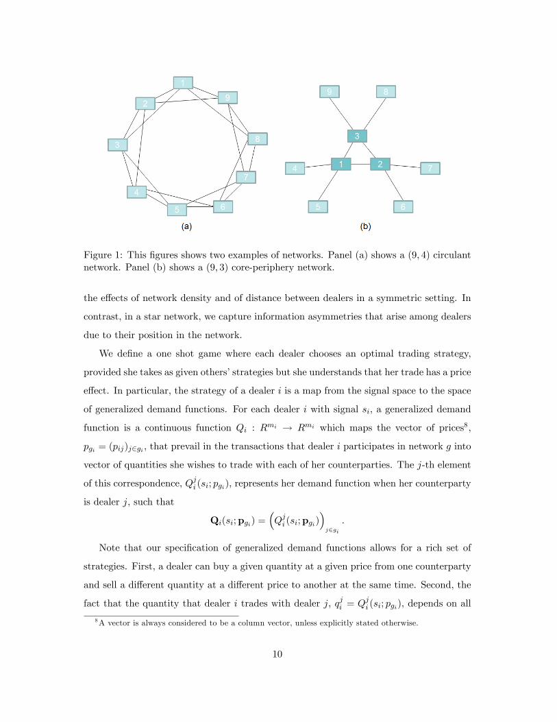
Figure 1: This figures shows two examples of networks. Panel (a) shows a (9, 4) circulantnetwork. Panel (b) shows a (9, 3) core-periphery network.

the effects of network density and of distance between dealers in a symmetric setting. In

contrast, in a star network, we capture information asymmetries that arise among dealers

due to their position in the network.

We define a one shot game where each dealer chooses an optimal trading strategy,

provided she takes as given others’strategies but she understands that her trade has a price

effect. In particular, the strategy of a dealer i is a map from the signal space to the space

of generalized demand functions. For each dealer i with signal si, a generalized demand

function is a continuous function Qi : Rmi → Rmi which maps the vector of prices8,

pgi = (pij)j∈gi , that prevail in the transactions that dealer i participates in network g into

vector of quantities she wishes to trade with each of her counterparties. The j-th element

of this correspondence, Qji (si; pgi), represents her demand function when her counterparty

is dealer j, such that

Qi(si; pgi) =(Qji (si; pgi)

)j∈gi

.

Note that our specification of generalized demand functions allows for a rich set of

strategies. First, a dealer can buy a given quantity at a given price from one counterparty

and sell a different quantity at a different price to another at the same time. Second, the

fact that the quantity that dealer i trades with dealer j, qji = Qji (si; pgi), depends on all

8A vector is always considered to be a column vector, unless explicitly stated otherwise.

10

the prices pgi , captures the potential interdependence across all the bilateral transactions

of dealer i. For example, if k is linked to i who is linked to j, a high demand from dealer

k might raise the bilateral price pki. This might make dealer i to revise her estimation of

her value upwards and adjust her supplied quantity both to k and to j accordingly. Third,

the fact that Qji (si; pgi) depends only on pgi but not on the full price vector emphasizes

the critical feature of OTC markets that the price and the quantity traded in a bilateral

transaction are known only by the two counterparties involved in the trade and are not

revealed to all market participants. Fourth, the fact that dealers choose demand schedules

implies that dealers effectively bargain both over prices and quantities. This has a crucial

role in our results. It is also in contrast with most other models of OTC markets where

the traded quantity is fixed and agents bargain only over the price.

Apart from trading with each other, dealers also serve a price-sensitive customer base.

In particular, we assume that for each transaction between i and j the customer base

generates a downward sloping demand

Dij(pij) = βijpij , (1)

with an arbitrary constant βij < 0. In our analysis costumers play a pure technical role:

the exogenous demand (1) ensures the existence of the equilibrium.9

The expected payoff for dealer i with signal si corresponding to the strategy profile

{Qi (si; pgi)}i∈{1,...,n} is

E

∑j∈gi

Qji (si; pgi) (θi − pij) |si

where pij are the elements of the bilateral clearing price vector p defined by the smallest

element of the set

P({Qi (si; pgi)}i , s

)≡{

p∣∣∣ Qji (si; pgi) +Qji

(sj ; pgj

)+ βijpij = 0, ∀ ij ∈ g

}9 It has been known since Kyle (1989) that with only two trading agents there is no linear equilibrium

in a demand submission game. This is not different under our formulation. We follow Vives (2011) andintroduce an exogenous demand curve to overcome this problem. This assumption has a minimal effecton our analysis. As we show in Corollary 1, prices and beliefs do not depend on βij and quantities scalelinearly even when βij → 0.

11

by lexicographical ordering10, if P is non-empty. If P is empty, we pick p to be the infinity

vector and say that the market brakes down and define all dealers’payoff to be zero. We

refer to the collection of these rules defining a unique p for any given signal and strategy

profile as p = P({Qi (si; pgi)}i , s

).

2.2 Equilibrium Concept

The environment described above represents a Bayesian game, henceforth the OTC game.

The risk-neutrality of dealers and the normal information structure allows us to search for

a linear equilibrium of this game defined as follows.

Definition 1 A Linear Bayesian Nash equilibrium of the OTC game is a vector of linear

generalized demand functions {Q1(s1; pg1),Q2(s2; pg2), ...,Qn(sn; pgn)} such thatQi(si; pgi)

solves the problem

max(Qji )j∈gi

E

∑j∈gi

Qji (si; pgi) (θi − pij)

|si (2)

where p = P (·, s).

A dealer i chooses a demand function for each transaction ij, in order to maximize

her expected profits, given her information, si, and given the demand functions chosen

by the other dealers. Then, an equilibrium of the OTC game is a fixed point in demand

functions.

3 The Equilibrium

In this section, we derive the equilibrium in the OTC game. We proceed in steps. First, we

derive the equilibrium strategies as a function of posterior beliefs. This step is standard.

Second, we solve for posterior beliefs. For this, we introduce an auxiliary game in which

dealers, connected in the same network and operating in the same informational environ-

ment as in the OTC game, do not trade. Instead, they make a best guess of their own

value conditional on their signals and the guesses of the other dealers they are connected

10The specific algorithm we choose to sellect a unique price vector is immaterial. We just have to ensurethat our game is well defined even for strategies which are allowed, but never part of the equilibrium.

12

to. We label this structure the conditional-guessing game. Third, we establish equivalence

between the posterior beliefs in the OTC game and those in the conditional-guessing game

and provide suffi cient conditions for existence of the equilibrium in the OTC game for any

network. We discuss the main properties of the equilibrium in Section 4.

3.1 Derivation of demand functions

Our derivation follows Kyle (1989) and Vives (2011) with the necessary adjustments. We

conjecture an equilibrium in demand functions, where the demand function of dealer i in

the transaction with dealer j is given by

Qji (si; pgi) = bjisi +(cji

)Tpgi (3)

for any i and j, where (cji) = (cjik)k∈gi .

As it is standard in similar models, we simplify the optimization problem of (2) which

is defined over a function space, to finding the functions Qji (si; pgi) point-by-point. That

is, for each realization of the signals, s, we solve for the optimal quantity qji that each

dealer i demands when trading with a counterparty j. The idea is as follows. Given the

conjecture (3) and market clearing

Qji (si; pgi) +Qij(sj ; pgj ) + βijpij = 0, (4)

the residual inverse demand function of dealer i in a transaction with dealer j is

pij = −bijsj +

∑k∈gj ,k 6=i c

ijkpjk + qji

ciji + βij. (5)

Denote

Iji ≡ −

bijsj +∑

k∈gj ,k 6=icijkpjk

/(ciji + βij

)(6)

and rewrite (5) as

pij = Iji −1

ciji + βijqji . (7)

13

The uncertainty that dealer i faces about the signals of others is reflected in the random

intercept of the residual inverse demand, Iji , while her capacity to affect the price is

reflected in the slope −1/(ciji + βij

). Thus, the price pij is informationally equivalent to

the intercept Iji . This implies that finding the vector of quantities qi = Qi(si; pgi) for one

particular realization of the signals, s, is equivalent to solving

max(qji )j∈gi

E

∑j∈gi

qji

(θi +

1

ciji + βijqji − I

ji

)|si,pgi

or

max(qji )j∈gi

∑j∈gi

qji

(E (θi|si,pgi) +

1

ciji + βijqji − I

ji

).

From the first order conditions we derive the quantities qji for each link of i and for each

realization of s as

21

ciji + βijqji = Iji − E (θi|si,pgi) .

Then, using (7), we can find the optimal demand function

Qji (si; pgi) = −(ciji + βij

)(E(θi |si,pgi )− pij) (8)

for each dealer i when trading with dealer j.

At this point we depart from the standard derivation. The standard approach is to

determine the coeffi cients in the demand function (3) as a fixed point of (8), given that

E(θi |si,pgi ) can be expressed as a function of coeffi cients bji and cji. This procedure is

virtually intractable for general networks. Instead, our approach is to solve directly for

the beliefs in the OTC game. In fact, we can find the equilibrium beliefs in the OTC game

without considering the profit motives and the corresponding trading strategies of agents.

For this, in the next section we specify an auxiliary game labeled the conditional-guessing

game.

14

3.2 The conditional-guessing game

The conditional guessing game is the non-competitive counterpart of the OTC game.

The main difference is that instead of choosing quantities and prices to maximize trading

profits, each agent aims to guess her value as precisely as she can. Importantly, agents are

not constrained to choose a scalar as their guess. In fact, each dealer is allowed to choose

a conditional-guess function which maps the guess of each of her neighbors into her guess.

Formally, we define the game as follows. Consider a set of n agents that are connected

in the same network g as in the corresponding OTC game. The information structure is

also the same as in the OTC game. Before the uncertainty is resolved, each agent i makes

a guess, ei, about her value of the asset, θi. Her guess is the outcome of a function that

has as arguments the guesses of other dealers she is connected to in the network g. In

particular, given her signal, dealer i chooses a guess function, Ei, which maps the vector

of guesses of her neighbors, egi , into a guess ei. When the uncertainty is resolved, agent i

receives a payoff

− (θi − ei)2 .

Definition 2 An equilibrium of this game is given by a strategy profile (E1, E2, ..., En) such

that each agent i chooses strategy Ei : R × Rmi → R in order to maximize her expected

payoff

maxEi

{−E

((θi − ei)2 |si

)},

where ei is the guess that prevails when

ei = Ei (egi) (9)

for all i ∈ {1, 2, ..., n}.

We assume that if a fixed point in (9) did not exist, then dealers would not make any

guesses and their profits would be set to minus infinity. Essentially, the set of conditions

(9) is the counterpart in the conditional-guessing game of the market clearing condition

in the OTC game.

15

As in the OTC game, we simplify this optimization problem and find the guess func-

tions Ei (si; egi) point-by-point. The procedure is as follows. An agent i chooses a guess

function that maximizes her expected profits, given her information, si, and given the

guess functions chosen by the other agents evaluated at the fixed point determined by the

set of conditions (9). Moreover, her guess function must be optimal for each realization of

the other dealers’signals sj , as it is reflected in the vector of guesses egi . Therefore, her

optimal guess is then given by

ei = E (θi|si, egi) . (10)

In the next proposition, we state that the guessing game has an equilibrium in any

network.

Proposition 1 In the conditional-guessing game, for any network g, there exists an equi-

librium in linear guess functions, such that

Ei (si, egi) = yisi + zgiegi

for any i, where yi is a scalar and zgi = (zij)j∈gi is a row vector of length mi.

It is easy to see that a collection of expectations ei satisfying (10) for all i, must be a

linear combination of the signals

ei = vis,

where vi is a row vector of length n. Therefore, we can think of the conditional guessing

game as a standard fixed point problem in the space of n× n matrices. For example, let

us pick an arbitrary row vector v0i of size n, for each agent i and conjecture that the guess

of agent j is

e0j = v0

js. (11)

Given that this conjecture describes the guesses of each of the neighbors of dealer i, her

best conditional guess for θi minimizing E(

(θi − ei)2 |si)is

e1i = E

(θi|si, e0

gi

). (12)

16

Since each element of e0gi is a linear function of the signals and the conditional expectation

is a linear operator for jointly normally distributed variables, E(θi|si, e0

gi

)determines a

unique vector v1i which can satisfy

e1i = v1

i s. (13)

This holds for every agent, and the the n× n matrix V 0 =[v0i

]i=1,..n

is mapped to a new

matrix of the same size V 1 =[v1i

]i=1,..n

. We show that this mapping has a fixed point.

An equilibrium of the conditional guessing game is given by the coeffi cients of si and egi

in E (θi|si, egi) at this fixed point.

In the next section we establish an equivalence between the equilibria of the OTC

game and the conditional guessing game. Therefore, in Section 4, we will be able to use

the properties of the conditional guessing game to learn about beliefs in the OTC game

3.3 Equivalence and existence

In this part we prove the main results of this section. First, we show that if there exists a

linear equilibrium in the OTC game then the posterior expectations form an equilibrium

expectation vector in the corresponding conditional guessing game. Second, we provide

suffi cient conditions under which we can construct an equilibrium of the OTC game build-

ing on an equilibrium of the conditional guessing game.

Proposition 2 In any Linear Bayesian Nash equilibrium of the OTC game the vector

with elements ei defined as

ei = E(θi |si,pgi )

is an equilibrium expectation vector in the conditional guessing game.

The idea behind this proposition is as follows. We have already showed that in a linear

equilibrium demand functions are given by (8). Substituting this into the bilateral market

clearing condition (4) gives

pij =

(ciji + βij

)E(θi |si,pgi ) +

(cjij + βij

)E(θj

∣∣si,pgj )

ciji + cjij + 3βij,

17

implying that a price pij is a linear combination of the posteriors of i and j, E(θi |si,pgi )

and E(θj∣∣sj ,pgj ). Therefore, a dealer can infer the belief of her counterparty from the

price, given that she knows her own belief. When choosing her generalized demand func-

tion, she essentially conditions her expectation about the asset value on the expectations

of the other dealers she is trading with. Consequently, the set of posteriors that the OTC

game implies works also as an equilibrium in the conditional guessing game.

Proposition 3 Let yi and zgi = (zij) the coeffi cients that support an equilibrium in the

conditional-guessing game and let ei = E(θi |si, egi ) the corresponding equilibrium expecta-

tion of agent i. Then, there exists a Linear Bayesian Nash equilibrium in the OTC game,

whenever ρ < 1 and the following system

yi(1−

∑k∈gi

zik2−zki

4−zikzki

) = yi (14)

zij

2−zij4−zijzji(

1−∑k∈gi

zik2−zki

4−zikzki

) = zij ,∀j ∈ gi

has a solution {yi, zij}i=1,..n,j∈gi such that zij ∈ (0, 2). The equilibrium demand functions

are given by (3) with

bji = −βij2−zji

zij+zji−zijzji yi

cjij = −βij2−zji

zij+zji−zijzji (zij − 1)

cjik = −βij2−zji

zij+zji−zijzji zik.

(15)

and the equilibrium prices and quantities are

pij =

(ciji + βij

)ei +

(cjij + βij

)ej

cjij + ciji + 3βij(16)

qji = −(ciji + βij

)(ei − pij) . (17)

Note that these two propositions prove the equivalence between our two games in both

directions. Proposition 2 shows that one can construct an equilibrium of the conditional

guessing game from an equilibrium of the OTC game. Proposition 3 shows that, under

18

some conditions, the reverse also holds. The extra conditions are a consequence of the fact

that in the reverse direction we are transforming n expectations, ei, from the conditional

guessing game into M ≥ n prices in the OTC game. The conditions make sure that we

can do it in a consistent way. While we do not have a general proof that this condition

holds for any network, we have no reason to suspect that it does not hold.11

The next proposition strengthen the existence result for our specific examples.

Proposition 4 1. In any network in the circulant family, the equilibrium of the OTC

game exists.

2. Whenever zij ∈ [0, 1] , then for any network in the core-periphery family, the equi-

librium of the OTC game exists.

The conceptual advantage of our way of constructing the equilibrium over the standard

approach is that it is based on a much simpler and, as we will see in the next section,

much more intuitive fixed point problem. Note also that Proposition 3 also describes a

simple numerical algorithm to find the equilibrium of the OTC game for any network.12

In particular, the conditional guessing game gives parameters yi and zij , conditions (14)

imply parameters yi and zij , then (15) give parameters of the demand function implying

prices and quantities by (16)-(17).

Before proceeding to the detailed analysis of the features of the equilibrium in the next

section, we make three simple observations.

First, the equivalence of beliefs on the two games implies that any feature of the

beliefs in the OTC game must be unrelated in any way to price manipulation, imperfect

competition or other profit related motives. It is so, because these considerations are not

present in the conditional guessing game.

Second, the equilibrium coeffi cients both in the conditional guessing game and in the

OTC game depend only on the ratio σ2θσ2εand not on the individual parameters σ2

ε and σ2θ.

11Our numerical algorithm gives a well behaving solution in all our experiments including a wide rangeof randomly generated networks. In Appenedix C, we also give analytical expressions for the equilibriumobjects in some specific networks.12The Matlab code runs in a fraction of a second for any network we experimented with and it is available

from the authors.

19

We state this result in the following Lemma.13

Lemma 1 The coeffi cients vij , zij , yi, zij , yi, bji , c

jij and c

jik do not change in σ

2ε and σ

2θ if

σ2θσ2εremains constant.

Finally, consumers’demand has a pure technical role in our analysis. While there is no

equilibrium for βij = 0, for any βij < 0 prices and beliefs are the same and qjiβij,qijβijremain

constant. This is evident by simple observation of expressions (16)- (15). We summarize

this in the following Corollary.

Corollary 1 For any collection of non-zero{βij}ij∈g including the limit where all βij →

0, prices, pij and beliefs do not change and quantities scale linearly. That is

qjiβij

,qijβij

do not change with βij .

4 Characterization and discussion

In this section, we analyze the properties of the equilibrium. First, we start with a re-

view of the centralized market benchmark, the Vives (2011) model. Then we proceed to

the discussion of how the decentralized trading environment affects prices, volume and

intermediation. In the last part, we focus on information transmission through trading.

4.1 A benchmark: the centralized market

When trade takes place in a centralized market, our environment collapses to the risk-

neutral case in Vives (2011). The main difference in his model compared to ours is that

in a centralized market agents submit simple demand functions to a market maker and

the market clears at a single price. For completeness, we summarize the properties of the

equilibrium in centralized markets in the following proposition. The derivation follows the

13Note that the Lemma does not imply that any economic objects depend only on the ratio of σ2ε

σ2θ. For

example, it is easy to see that for expected volume this is not the case.

20

standard approach that we described in Section 3.1 and the interested reader can find it

in Vives (2011).

Proposition 5 (Vives, 2011) Let be ρ < 1. In a centralized market there is a linear

demand function equilibrium if and only if

n− 2 <nρσ2

ε

(1− ρ)(σ2ε + (1 + (n− 1) ρ)σ2

θ

) . (18)

The demand functions and the price are given by

Qi(si; p) = − (c+ (n− 1)β) (E (θi|si, p)− p) = bsi + cp (19)

p =(nc+ n (n− 1)β)

nc+ n (n− 1)β + β

1

n

n∑i=1

E (θi|si, p) (20)

where β is the slope of the exogenous demand curve and

c = β(1− ρ)

(σ2ε + (1 + (n− 1) ρ)σ2

θ

)− ρσ2

ε

(n− 2) (1− ρ)(σ2ε + (1 + (n− 1) ρ)σ2

θ

)− nρσ2

ε

(21)

b =(1− ρ)σ2

θ

(1− ρ)σ2θ + σ2

ε

(−β − c (n− 1)) .

The price is fully privately revealing in the sense of

E (θi|si, p) = E (θi|s) .

The first thing to note is that in centralized markets the price is always fully privately

revealing. As we will discuss in length in part 4.3, this is typically not the case in a

decentralized market

However, this benchmark also highlights a few important insights which are partially

or fully inherited by our structure. Just as in our case, there are gains from trade whenever

ρ < 1. As the price is close to the average valuation of agents, the first expression in (19)

implies that agents with higher than average signals (optimists) tend to buy and agents

with lower than average signals (pessimists) tend to sell the asset. In fact, given that

21

agents are risk-neutral, two critical features prevent optimists and pessimists from taking

infinite positions. The first feature is that dealers can learn from prices and the second

one is that they take into account that their trade has a price effect. To see this, note that

comparing the two expressions for agents demand in (19) gives

c = ((n− 1) c+ β) (1− z) (22)

where z is the coeffi cient of price in the conditional expectation

E (θi|si, p) = ysi + zp.

That is, the slope, c, of the demand curve of a given dealer is the product of the inverse of

her price effect (given that all the other agent have a slope of c) and an inverse measure

of the informational content of prices, (1− z). If dealers were price takers or they did not

care about the information content of prices, there would be no equilibrium with finite

quantities.

From (21), it is clear that larger ρ, σ2ε or smaller σ

2θ increases c (i.e., typically decreases

its absolute value). This is an instance of the well known result since Akerlof (1970) that

adverse selection limits trade. All these changes of parameters imply that a given agent

finds the signals of others more informative for the estimation of her own valuation.14

For example, suppose that a dealer with high initial beliefs considers to buy. If many

other dealers desire to sell at the same time, pushing prices downward, the first dealer

typically increases her demand as a response. However, this adjustment will be weaker, if

she is worried that the large supply indicates a low value for the asset. The stronger the

information content of other agents’signals, the smaller the quantity response, i.e., the

absolute value of c. It turns out that when adverse selection is not strong enough there is

no solution in (22). This is the intuitive content of condition (18). As ρ and σ2ε decrease

or σ2θ increases, the informational content in others’ signals decreases and as condition

14 In fact, there are two opposite forces at work when σ2ε decreases. It makes the dealer’s own signalmore precise, decreasing the relevant information content in prices, but at the same time it makes all otherdealers’signals more precise, increasing the relevant information content in prices. However, the first effectalways dominates, because the effect of the others’signals largely cancels out when they are averaged.

22

(18) gets binding, adverse selection limits trade less and less and (−c) increases without

bounds.

In the next part, we discuss to what extent the mechanism of price formation and

trading volume changes in a decentralized market.

4.2 Price dispersion, volume and intermediation

Just as in the centralized market benchmark, it is the interdependent value environment

with ρ < 1 that ensures that agents trade in our case. Also, the interaction of adverse

selection and imperfect competition is still the force which prevents agents from taking

infinite positions. However, there are also important differences implied by our structure.

As an illustration, we consider a numerical example with the simplest possible network

depicted on Figure 2. There are three dealers organized in a (2, 1) core-periphery network

(also known as a line and a 3-star) depicted by the connected squares. For simplicity, we

index them by their position: L(eft), C(entral), R(ight). The number in each square is

the realization of their signal; sL = −2, sC = 0, sR = 1. We picked βL,C = βR,C = β = −5.

Prices are in the rhombi located on the links and demand curves are at the bottom of the

figure in the form

qji = tji (E(θi |si,pgi )− pij) (23)

where tji ≡ −(ciji + βij

)is the trading intensity of trader i when trading with counterparty

j. This corresponds to the interpretation that agent i trades tji units with counterparty j

for every unit of perceived gain, E(θi |si,pgi ) − pij . Just for this example, we omit the

superscript to simplify the exposition and use tL, tC , tR for the trading intensities of L,C

and R respectively (i.e., tL = tR = 10.8 and tC = 10.5). Substituting in the prices and

signals gives the traded quantities in the first line of the rectangles. Below the quantities

in brackets, we calculated the profit or loss realized on that particular trade in the case

when the realized value, θi, is zero for all dealers. All quantities are rounded to the nearest

decimal. For example, the central dealer forms the posterior expectation of −1, buys 3

units from the left and sells 2.4 units to the right at prices −0.4 and 0.1 respectively,

earning 2.9 unit of profit in total in the trades. Note, that while counterparties hold a

23

position of opposite sign and same order of magnitude, bought and sold quantities over

a given link does not add up to 0. It is so, as the net of the two positions is sold to the

customers.

Figure 2: The connected squares depict three dealers organized in a (2, 1)-core-peripherynetwork. Their realized signals are in the middle of the square. Prices are in rhombi,demand curves are at the bottom of the figure, with the posterior expectations in italic.The traded quantities are in the first line of the rectangles. Below, the profit or lossrealized on that particular trade in the case when θi = 0 for all i.Parameters are ρ =−.5, σ2

θ = σ2ε = 1, βij = −5.

There are a number of observations which generalize to other examples. First, price

dispersion arises naturally in this model. The central dealer is trading the same asset

at two different prices, because she is facing two different demand curves. Just as a

monopolist does in a standard price-discrimination setting, the central agent sets a higher

price in the market where demand is higher. In fact, from (16), we can foresee that the

price dispersion in our framework must be closely related to the dispersion of posterior

beliefs.

Second, profitable intermediation by central agents also arises naturally. That is, the

central dealer’s net position (3−2.4) is significantly lower than her gross position (3+2.4)

as she trades not only to take a speculative bet but also to intermediate between her

counterparties.

Third, the decentralized structure introduces a natural asymmetry in trading. That

24

is, even if all dealers have the same quality of information, trading intensities are different.

To see this, consider the decentralized version of equation (22) coming from (8) describing

the best response slope cCL,C of dealer L in transaction with C to the same slope of dealer

C, cLC,L

cCL,C =(cLC,L + β

)(1− zL) . (24)

where zL is the coeffi cient of the price between C and L, pL,C in the expectation E(θL|sL, pL,C).

Using our definition of (23), we rewrite this expression15 and the corresponding one on

cLC,L as

−tC = tL (zL − 1) + β

−tL = tC (zC − 1) + β

or

tC = −β 2− zLzC + zL − zLzC

tL = −β 2− zCzC + zL − zLzC

.

Clearly, the reason behind the trading intensity of the central agent being smaller than

that of the other agents must be that the central agent relies on each price as a source of

learning less than the others, zL = zR > zC . Indeed, this is the case, as the central agent

can learn from two prices. Therefore, she is less subject to adverse selection. Thus, an

extra unit sold by the left agent triggers a smaller price-adjustment by the central agent

inducing the left agent to trade more aggressively. This explains tL > tC .

Fourth, we can understand the joint determination of quantities and prices at each

link as the outcome of a fictional bargaining process. To see this, using (16) and (23) we

rewrite the price between L and C as a weighted average of the posterior expectations of

15 In E(θC |sC , pL,C , pR,C) the coeffi cients of the two prices are equal. Thus, with a slight abuse ofnotation we denote both zC in this simple example.

25

L, C and 0 (the bliss point of customers)

pL,C =tLeL + tCeC + (−β) 0

tL + tC + (−β).

The expression for the price between R and C is analogous. This expression shows that

the more aggressive an agent trades, the closer the price is to her expectation, decreasing

her perceived per-unit profit |ei − pij |. Intuitively, in our example, the pessimistic agent

prefers to sell assets to the center agent with larger trading intensity than the trading

intensity the central agent is willing to buy with. As markets has to clear, the only way

they can agree on the terms, if the pessimistic agent, L, gives a price concession to agent

C.

Note also, that in this simple example while the slope of the demand curves differ across

dealers, the slope of the demand function of the central dealer is the same when trading

with each of her counterparties. This does not has to be the case. Even in symmetric

networks, such as the family of circulants, dealer i’s demand functions has a different slope

depending whom she is trading with. We illustrate this on Figure 3.16 This suggests that

the price effect of an additional unit traded over the counter depends on the particular

pair of dealers that are transacting.

Finally, note that in the decentralized case there can be an equilibrium even if ρ or σ2ε

is very small. That is, in the decentralized case there is no analogous condition to (18).

This is a consequence of trade being bilateral.

In Appendix B we provide more examples involving other networks to illustrate the

effects of these observations.

4.3 Prices and information transmission

In this part we focus on the characteristics of equilibrium beliefs in OTC games and its

implications on the informational effi ciency of prices.

We start with two results on the equilibrium of the conditional guessing game.

16 In figure 3, for simplification, we normalize the slope with the size of outside demand and plot cjij/βij ,as this ratio is independent of βij .

26

Figure 3: The figure shows the slope,cj1jβ1j

of the demand curve, Qj1 submitted by agent 1 for

the trade where the counterparty is j in the (11,m) circulant networks. Other parametersare σ2

ε = σ2θ = 1, ρ = 0.5.

Lemma 2 In the conditional guessing game the following properties hold.

1. In any connected network g each dealer’s equilibrium guess is a linear combination

of all signals

ei = vis,

where vi is a row vector of length n and vi > 0.

2. In any connected network g when ρ = 1, there exists an equilibrium where each

element of the vectors vi is equal toσ2θ

nσ2θ+σ2ε. In this equilibrium each expectation

effi ciently aggregates all the private information in the economy.

3. Any equilibrium of the conditional game depends on σ2ε and σ

2θ only through the ratio

σ2εσ2θ.

As we will argue, in the OTC game the following corresponding claims also hold.

Proposition 6 Suppose that there exists an equilibrium in the OTC game. Then,

27

1. in any connected network g each bilateral price is a linear combination of all signals

in the economy, with a positive weight on each signal;

2. in any connected network g prices are privately fully revealing when ρ→ 1, as

limρ→1

(V (θi|si,pgi)− V (θi|s)) = 0.

These results suggest that a decentralized trading structure can be surprisingly effec-

tive in transmitting information. Consider first result 1 of the Proposition 6. This shows

that although we consider only a single round of transactions, each price partially incor-

porates all the private signals in the economy. A simple way to see this is to consider the

residual demand curve and its intercept, Iji , defined in (6)-(7). This intercept is stochastic

and informationally equivalent with the price pij . The chain structure embedded in the

definition of Iji is critical. The price pij gives information on Iji which gives some infor-

mation on the prices agent j trade at in equilibrium. For example, if agent j trades with

agent k then pjk affects pij . By the same logic, pjk in turn is affected by the prices agent k

trades at with her counterparties, etc. Therefore, pij aggregates the private information of

signals of every agent, dealer i is indirectly connected to, even if this connection is through

several intermediaries.

This property of the equilibrium does not imply that dealers learn all the relevant

information in the economy, as it happens in a centralized market. In particular, it follows

from Proposition 6 that in a network g, a dealer i can use only mi linear combinations of

the vector of signals, s, to infer (a suffi cient statistics of) the other (n− 1) signals. Except

in two special cases, this is generally not suffi cient for the dealer to learn all the relevant

information in the economy. One trivial special case is when each agent has mi = n − 1

neighbors, that is, when the network is complete. The second special case is highlighted as

result 2 in the Proposition 6. It claims that in the common value limit, the decentralized

structure does not impose any friction on the information transmission process in any

network. To shed more light on the intuition behind these results, we have to understand

better the learning process in the conditional guessing game.

Consider the case when ρ = 1. The expressions (11)-(13) can be seen as an iterated

28

algorithm to find the equilibrium of the conditional guessing game in an arbitrary network.

That is, in round 0 each agent i receives an initial vector of messages e0gi from her neighbors.

Given that, each of agent i chooses her best, e1i, guess as in (12). The vector of messages

e1gi given by (13) is the starting point for i in the following round. By definition, if this

algorithm converges to a fixed point, then this is an equilibrium of the conditional guessing

game. According to result 2 in Lemma 2, when ρ = 1, the equal-weighted sum of signals,σ2θ

nσ2θ+σ2ε1>s, is a fixed point. The reason is simple. With common values, σ2θ

nσ2θ+σ2ε1>s is

the best possible guess for each agent given the information in the system. In addition,

as the sum of signals is a suffi cient statistic, the expectation operator (12) keeps this

guess unchanged. Since the equilibrium of the conditional guessing game is continuos in

ρ, information is aggregated effi ciently also in the OTC game in the common value limit.

Clearly though, exactly at ρ = 1 there is no equilibrium by the Grossman paradox.

Now we depart from the common value limit case. In this case, information transmis-

sion is only partial. In particular, if agent k is located further from agent i, her signal is

incorporated to a smaller extent into agent i’s belief. To see the intuition, we apply the

iterated algorithm defined by (11)-(13) for the example of a circle-network of 11 dealers.

We illustrate the steps of the iteration in Figure 4.3 from the point of view of dealer 6.

We plot the weights with which signals are incorporated in the guess of dealer 5, 6 and 7.

In each figure the dashed lines show messages sent by dealer 5 and 7 in a given round, and

the solid line shows the guess of agent 6 given the messages she receives. In round 0, we

start the algorithm from the common value limit, σ2θnσ2θ+σ2ε

1T s, illustrated by the straight

dashed lines that overlap in panel A. When ρ < 1, in contrast to the common value limit,σ2θ

nσ2θ+σ2ε1T s is not a best guess of θ6 anymore. The reason is that dealer 6’s own signal,

s6, is more correlated to her value, θ6, than the rest of the signals are. Therefore, the

best guess of dealer 6 is a weighted sum of the two equal-weighted messages and her own

signal. This is shown by the solid line peaking at s6 in Panel A. Clearly, this is not a fixed

point as all other agents choose their guesses in the same way. Thus, in round 2, agent

6 receives messages that are represented by the dashed lines shown on Panel B; these are

the mirror images of the round-1 guess of dealer 6. Note that these new messages are less

informative for dealer 6 than the equal-weighted messages σ2θnσ2θ+σ2ε

1T s. The reason is that

29

even when ρ < 1, for dealer 6 the average of the other 10 dealers’signals is a suffi cient

statistic for her about all the information which is in the system apart from her own signal,

which she observes anyway. So from the round−0 messages, she could learn everything she

wanted to learn. From the round−1 messages she cannot. The extra weight that dealer

5 and 7 place on their own private signals jams the information content of the messages

for dealer 6. Nevertheless, the round−2 messages are informative, and dealer 6 puts some

positive weight on those, and a larger weight on her own signal as the solid line on Panel

B shows. This guess has a "kink" at s5 and s7, because in this round dealer 6 conditions

on messages which overweight these two signals. Since all other agents choose their guess

in a similar way in round 2, the messages that dealer 6 gets in round 3 are a mirror image

of her own guess, as shown by the dashed lines in Panel C. The solid line in Panel C

represents dealer’s 6 guess in round 4. On Panel D, we depict the guess of dealer 6 in each

round until round-5, where we reach the fixed point. Note that it has all the properties

we claimed: positive weight on each agents’signals, but decreasing in the distance from

dealer 6.

Away from the common value limit, information transmission is not even "constrained

informationally effi cient". That is, dealers’ equilibrium guesses are different than the

solution to the problem of a planner searching for the linear functions {Ei (si, egi)}i=1...n

which minimize the expected sum of squared errors

E

[∑i

(θi − ei)2

]

subject to (9). To see this, we continue the previous example by comparing the equilibrium

guess with the solution of the planner’s problem on Figure 5. As it is apparent, dealers

put too much weight on their own signal from a social learning point of view. The reason

is clear from the above explanation. When dealers’distort messages towards their own

signals, they do not internalize that they reduce the information content of these guesses

for others.

By Proposition 3, the properties of prices in the OTC game are implied by the proper-

ties of the equilibrium in the conditional guessing game. That is, the correlation between

30

Figure 4: An iterated algorithm to find the equilibrium of the conditional guessing gamein a 11-circle. Each line shows weights on a given signal in a given message or guess.Dashed lines denote messages dealer 6 recevies from her contacts of dealer 5 and 7, andthe solid line denotes her best response guess of her value. Panel A,B,C illustrates round1,2 and 3 of iteration, respectively, while panel D illustrates all rounds until convergence.Parameters are n = 11, ρ = −.8, σ2

θ = σ2ε = 1, βij = −10

11 .

prices pij and pkl tend to be lower if the link ij is further from kl. Also, prices could trans-

mit more information even within the constraint imposed by our network structure. From

the intuition gathered from the conditional guessing game, it is clear that this distortion

is not a result of imperfect competition, strategic trading or anything else connected to

the profit motives of agents. Instead, it is a consequence of the learning externality aris-

ing from the interaction between the interdependent value environment and the network

structure of information sharing.

4.4 Applications: Theory and facts

An attractive feature of our model is that it generates a rich set of empirical predictions.

Namely, for any given information structure and dealer network, our model generates

31

Figure 5: The solid curve depicts the equlibrium weights on each of the signals of dealer 6in the conditional guessing game, v6. The dashed curve shows the weights in the solutionminimizing the expected total squared errors of guesses for all i. Parameters are n = 11,ρ = −.8, σ2

θ = σ2ε = 1, βij = −10

11 .

the full list of demand curves and the joint distribution of bilateral prices and quanti-

ties, and measures of price dispersion, intermediation, trading volume etc. Therefore,

one can directly compare our results to the stylized facts described by the growing em-

pirical literature using transaction level OTC data. In this way, our model can help to

decide whether dealer’s assymmetric information can or cannot be behind stylized facts

in particular markets, during particular episodes

To illustrate this feature, we present two simple exercises. First, we highlight the ex-

pected relationship between the cost of trading, price dispersion, size of trades and certain

properties of the given asset, if the main driving force of trading is dealer’s asymmetric

information. Second, we confront narratives on the potential mechanisms behind OTC

market distress to the observed stylized facts emerging from existing empirical analyses.

4.4.1 Trading cost, price dispersion and transaction size

In this part our main objects of interest are trading cost and price dispersion. We picked

the former because of its dominant role in the empirical literature and the latter because

32

price dispersion is a characteristic feature of OTC markets.

The majority of the empirical literature conceptualizes trading cost (also referred to

as mark-up or effective spread) as the cost of selling and instantaneously buying back a

given quantity as a fraction of the value of the transaction. This is the percentage cost of

a round-trip trade. In particular, Green, Hollifield and Schurhoff (2007), Edwards, Harris

and Piwowar (2007) and Li and Schürhoff (2012) showed that this cost is decreasing in

the size of the transaction. Also, Edwards, Harris and Piwowar (2007) and Bao, Pan

and Wang (2011) showed that this cost is smaller for higher rated corporate bonds. We

explain how these observations are consistent with our model and also derive additional

predictions.17

We can construct the theoretical counterpart of the percentage cost of a round-trip

trade as follows. Let us consider the difference of the price, pBij , at which trader i could buy

a quantity qji from trader j, and the price, pSij , at which i could sell the same quantity to

j and normalize this by the value of the transaction for i given her fundamental valuation

θi

pBij − pSijqji θi

=−bijsj+

∑k∈gj ,k 6=i

cijkpjk+qji

ciji+βij+

bijsj+∑k∈gj ,k 6=i

cijkpjk−qji

ciji+βij

qji θi=

2(ciji + βij

)θi, (25)

where we used (5). We refer to this measure as the cost of trading.

To see what properties we should expect from a data-set generated by our model, let us

consider the following exercise. We fix the network and take a given realization of signals.

Our model generates a list of transactions with varying characteristics for each linked

dealer-pairs. This is a cross-section of transactions. Then we can change the realized

signals, generate another cross-section and think of this as the data corresponding to the

next time-period. Repeating this, we obtain a series of transactions with different size

and price for each dealer-pair. Thus, we can think of the complete data-set as a panel

17The only paper to our knowledge which directly connects the characteristics of the transactions tothe position of the dealer in the network is Li and Schürhoff (2012). Consistently with the features inour model, the authors show that central agents trade more and seem to be better informed than others.However, they also show that central agents trade at a higher percentage cost. This is not consistent in ourmodel implying that, at least in that particular market of municipal bonds, there are other determinantsof trading cost than adverse selection.

33

with both a cross-sectional and a time dimension. We can both treat this data at the

transaction level, or take averages of transactions belonging to a given dealer and treat it

at the dealer-level (counting each transaction twice).

It is apparent from (25) that for a fixed dealer-pair, the cost is independent of the

transaction size. This is a consequence of the linearity coming from our normally dis-

tributed information structure. However, in general(ciji + βij

)varies across dealer pairs.

Comparing (17) and (25) also shows that there must be an inverse relationship between

the cost of trading for agent i with j and the quantity she chooses to trade. Thus, if we

were to run a regression of the cost of the transaction to its size in our panel data set, we

would get a different result depending on our controls. Including dealer-pair fixed effects,

we would get no relationship at all. However, including time fixed effects, we would get

a strong negative relationship. Often, the econometrician cannot observe the identity of

the traders only some of their characteristics. Then, as an intermediate case of the two

extremes, we predict the following patterns.

Hypothesis 1 In the cross-section of transactions, the percentage cost of the transaction

decreases in the size of the transaction.

Hypothesis 2 By conditioning on the characteristics of the participating dealers in a

bilateral transaction, the negative relationship between the transaction’s size and its cost

gets weaker.

The first hypothesis is consistent with the empirical results of Green, Hollifield and

Schurhoff (2007),Edwards, Harris and Piwowar (2007) and Li and Schürhoff (2012). To

our knowledge, the second remains to be tested.

Turning to price dispersion, note that our framework can capture two distinct concepts

of price dispersion. Thinking of the generated panel, we can think of the price variability

in the time-series dimension for a given dealer-pair. This we refer to as the price volatility

corresponding to the given dealer-pair. Second, thinking of the cross-sectional dimension

we can think of the price variability across the bilateral relationships. We refer to this

variation as price dispersion. More formally, consider the covariance matrix of prices in

each transaction, Σp. The diagonal elements of Σp is the right measure of price volatility,

34

while the off-diagonal elements of Σp represent the measure of price dispersion. A trans-

parent, normalized, single-value measure of the price dispersion across all dealer pairs is

the determinant of the correlation matrix of prices. The price dispersion across a specific

group of dealer-pairs can be measured as the determinant of the corresponding sub-matrix

of the correlation matrix.

As in real world the cross-sectional and time-dimensions of our hypothetical example

might not be fully separable (as each dealer-pair might not transact exactly once in each

date), empirically price dispersion and price volatility is closely related. However, in our

model these two objects are driven by different forces. Price volatility tends to be large in

those transactions in which dealers trade large quantities . This is so, because demand-

schedules are downward sloping implying larger price effects for large trades. As we argued

before, dealers with many connections are the ones who tend to trade a lot, therefore price

volatility will be largest for these pairs. In contrast, price dispersion tends to be small

across dealers who learn a lot from prices, because these dealers’posteriors are close and

prices are weigthed averages of posteriors. As the most connected dealers learn the most,

price dispersion will be small across dealer-pairs where both counterparties have many

connections. As those with many connections also trade the most, the following empirical

predictions follow.

Hypothesis 3 Price volatility is larger in those transactions in which dealers trade larger

quantities.

Hypothesis 4 Price dispersion is smaller across those transactions in which dealers trade

larger quantities.

The two hypothesis imply that even the sign of the relationship between price vari-

ability and transaction size can change depending on the measurement of price variability.

That is, the better the econometrician can control for the identity of the traders in the

transaction the observed prices corresponds to, our model predicts a more positive rela-

tionship.

Finally, let us consider how the cost, price dispersion and price volatility should change

across assets with different informational properties according to our model.

35

Note that Lemma 1 implies that the cost of trading depends on σ2ε and σ

2θ only through

the ratio of σ2θσ2ε. This ratio measures the relative precision of private information and we

will refer to it as the measure of information precision. As we discussed, in the centralized

model larger noise in the private signal of an agent (smaller information precision) increases

her reliance on the signals of others, increasing adverse selection and, consequently the

cost of trading. This property is preserved in our decentralized setting as well. While price

volatility and price dispersion depends both on σ2ε and σ

2θ in general, for simplicity here

we consider only the effect of the information precision on these objects. As the cost of

trading decreases with the information precision, the size of transactions and the resulting

price volatility also increases. Larger information precision also implies that agents learn

less from each other, making posteriors across agents more dispersed. That increases price

dispersion. The following hypothesis summarizes these observations.

Hypothesis 5 For asset classes where information precision tends to be higher, transac-

tion cost is smaller

Hypothesis 6 For asset classes where information precision tends to be higher, price

dispersion and price volatility are larger.

To the extent that information precision is lower for lower rated bonds, hypothesis 5 is

consistent with the empirical evidence in Edwards, Harris and Piwowar (2007) and Bao,

Pan and Wang (2011).

Note that Hypotheses 1-6 are not analytical results. For that, we need to take into

account how the size of the transactions between traders i and j depends jointly on the

coeffi cients and their posterior beliefs and how both of these depend on their position

in the network. Instead, we take a short-cut in forming these hypotheses based on the

intuition we developed in the previous sections and show extensive numerical simulations

to argue that they do hold regardless of the form of our network and the parameter values.

In particular, our framework allows for two simple ways to explore empirical predictions

for our model. First, one can choose a network with realistic features and explore the

connection with the stylized facts. Second, one can simulate a large number of random

36

Figure 6: A two-level core-perihpery network. Central dealers are red, mid-level dealersare blue and periphery dealers are green.

networks with random parameters and run regressions on various objects in this simulated

data set. We illustrate both of these options by the following exercises.

As a fixed network, we consider the 2-level core-periphery network depicted on Figure

6. This network has a core of three connected dealers who are linked with one mid-level

dealer each. Each mid-level dealer can intermediate between the core group and one other

dealer. Given the centralized structure of real-world OTC markets, this network is a simple

example to see how transactions within the core group differ from transactions between

core and mid-level dealers and mid-level and periphery dealers. Indeed, Figure 6 shows

the most important economic quantities as a function of information precision,σ2θσ2ε, for each

of these segments of the market. In line with the intuition embedded in (24), we see that

the core group trades with each other the most at the lowest percentage cost (spread)

as in those trades both party is the least worried about adverse selection. The multiple

connections of the core-group also implies that their posteriors as well as prices are the

least dispersed. In contrast, price volatility is largest for the core-group as they trade

the largest quantities. It is also apparent that as the information precision, σ2θσ2εincreases,

adverse selection is less severe for each group, decreasing the cost and increasing the size

of the transactions. However, the core-group is the least affected given that they are the

most connected of all. Putting together these observations imply our six [five] hypothesis.

37

Figure 7: Generalized dispersion (determinant of the sub-correlation matrix), spread (per-cantage cost), gross volume (expected sum of transaction size over each link of the dealer),and total expected profit in a two-level core-periphery network by the type of the coun-terparties as a function of uncertainty (σ

2ε

σ2θ).

38

We also run an extensive simulation where we generate 5000 random networks and pick

a random value for the noise in private information σ2ε. For simplicity, we use the Erdos-

Renyi algorithm where each link is formed with probability 12 . We record the expected

transaction size and cost as in (25) by transaction, the degree centrality (i.e. number

of links) of each counterparty, the information ratio σ2θσ2εand the asymmetry (standard

deviation of the degree distribution) of the network in a given run. We also record the

price volatility in each transaction and the dispersion of prices a given dealer trades at as

defined above. We keep the number of nodes at n = 11, and ρ = 0.5, σ2θ = 1.

Our results verifying our hypotheses 1-2 and 5 are in Table 4.4.1 The first column shows

a regression of the cost using only variables which should be observable in a transaction

based data-set, even if the identity of the traders are not recorded. In terms of our model,

this is a regression connecting the endogenous variables of volume and cost (and controlling

for the precision of private information). The second column shows the same regression

with controlling for a number of characteristics of the transacting dealers and the network.

Comparing coeffi cients of volume across regressions shows that all three hypotheses hold.

The third and the last column highlight the reason why volume and cost have a negative

association in our framework. This is because each of the exogenous characteristics are

related to volume with opposite sign then to cost.

Tables 4.4.1 and 4.4.1 show the results corresponding to hypotheses 3-4 and 6. Table

4.4.1 shows transaction level regressions on price volatility. The first two columns show

that price volatility is indeed associated with higher volume even after controlled for

network characteristics . The last column shows how price volatility is explained by the

primitives of our model as opposed to the endogenous variable of volume. Comparing

these coeffi cients with the last column of Table 4.4.1 explains the positive relationship

of trade and price volatility in our model as both objects are related to the exogenous

network characteristics of the counterparties the same way.

Finally, Table 4.4.1 contrast the behavior of price volatility and price dispersion in

our model. Given that price dispersion is not defined at the transaction level, Table 4.4.1

shows dealer-level regressions. For these regressions, the price volatility is the average

volatility of the prices a given trader trades at. The first two columns verify Hypothesis

39

cost cost cost volumevolume -0.0087∗∗∗ -0.0024∗∗∗

(-365.5039) (-162.9177)information -0.0003∗∗∗ -0.0009∗∗∗ -0.0011∗∗∗ 0.0853∗∗∗

(-17.9819) (-72.0536) (-84.7856) (52.6715)asym*other deg -0.0004∗∗∗ -0.0008∗∗∗ 0.1499∗∗∗

(-17.6554) (-29.6651) (42.957)asym.*own deg -0.0004∗∗∗ -0.0008∗∗∗ 0.1499∗∗∗

(-17.6782) (-29.6871) (42.9574)asymmetry 0.0092∗∗∗ 0.0133∗∗∗ -1.6198∗∗∗

(42.5303) (59.1098) (-61.3864)other degree -0.0047∗∗∗ -0.0048∗∗∗ 0.014∗∗

(-107.7905) (-103.6902) (2.5427)own degree -0.0051∗∗∗ -0.0051∗∗∗ 0.0148∗∗∗

(-115.6506) (-111.2389) (2.6857)R2 0.331 0.8 0.78 0.28N 274820 274820 274820 274820

Table 1: Regressions on a simulated dataset of expected transaction size (standardized), itspercentage cost of trade, number of links (degree) of each counterparty, standard deviation

of the degree distribution (asymmetry) and σ2θσ2ε(information, standardized) in 5000 random

network where each link forms with probability half with a randomly generated σ2ε value

in each. Standard OLS regressions with constants included (not reported) with t-stats inparenthesis. Remaining parameters are fixed at n = 11, ρ = 0.5 and σ2

θ = 1.

3-4 and 6. The third, fourth and columns connect dispersion, volatility and volume with

the network characteristics of dealers to shed more light where the sign of the coeffi cients

in the first two columns are coming from. In particular, we see that more connected dealers

in a more symmetric network trade at more volatile but less dispersed prices and the most

connected dealers in more asymmetric networks trade the most.

4.5 What goes wrong in OTC markets in a liquidity crisis?

An attractive feature of our model is that it gives a rich set of empirical predictions.

Namely, for any given information structure and dealer network, our model generates the

full list of demand curves and the joint distribution of bilateral prices and quantities, and

measures of price dispersion, intermediation, trading volume etc. Therefore, there is a

wide range of potential applications. For example, one could use our model as the main

40

price volatility price volatility price volatilityvolume 0.0129∗∗∗ 0.0032∗∗∗

(355.4973) (147.9372)information 0.0118∗∗∗ 0.0126∗∗∗ 0.0129∗∗∗

(324.9693) (689.348) (681.0835)asym*other deg 0.0008∗∗∗ 0.0012∗∗∗

(19.0934) (30.1043)asym.*own deg 0.0008∗∗∗ 0.0012∗∗∗

(19.0933) (30.1043)asymmetry -0.0157∗∗∗ -0.0208∗∗∗

(-52.8436) (-67.8771)other degree 0.0079∗∗∗ 0.008∗∗∗

(127.922) (123.806)own degree 0.0079∗∗∗ 0.008∗∗∗

(127.8815) (123.806)R2 0.48 0.87 0.86N 274820 274820 274820

Table 2: Regressions on a simulated dataset of price volatility, expected transaction size(standardized), number of links (degree) of each counterparty, standard deviation of the

degree distribution (asymmetry) and σ2θσ2ε(information, standardized) in 5000 random net-

work where each link forms with probability half with a randomly generated σ2ε value in

each. Standard OLS regressions with constants included (not reported) with t-stats inparenthesis. Remaining parameters are fixed at n = 11, ρ = 0.5 and σ2

θ = 1.

building block for the analysis of endogenous network formation given that our model

gives the payoffs for any given network. Alternatively, with a suffi ciently detailed data-set

in hand, one could use our framework for a structural estimation of the parameters in

different states of the economy. We leave these possibilities for future work. Instead, as

a simpler illustration of this richness, we confront narratives on the potential mechanisms

behind OTCmarket distress to the observed stylized facts emerging from existing empirical

analyses.

As a starting point, in the following table we summarize the findings of four recent

empirical papers that investigate the effect of a liquidity event on market indicators. We

focus on three indicators: price dispersion, price impact and volume.18

18The interested reader can find futher analyses on the effect of changing information structure onintermediation an profits in Appendix B.

41

dispersion price volatility dispersion price volatility volumevolume -0.0267∗∗∗ 0.0157∗∗∗

(-63.9095) (285.0991)information 0.0032∗∗∗ 0.0115∗∗∗ 0.0008∗∗ 0.0129∗∗∗ 0.0905∗∗∗

(7.5731) (208.9943) (2.0122) (316.917) ( 51.5954)degree -0.0253∗∗∗ 0.0113∗∗∗ 0.5727∗∗∗

(-100.9552) (437.4865) ( 513.7707)asymmetry 0.038∗∗∗ -0.0018∗∗∗ 0.3026∗∗∗

(29.0968) (-13.9264) (52.2741)R2 0.069 0.71 0.17 0.84 0.82N 55000 55000 55000 55000 55000

Table 3: Regressions on a simulated dataset of the average volatility of prices a given dealertrades at, the price dispersion (determinant of the correlation matrix) of these prices, thesum of the expected transaction size of a given dealer (standardized), number of links(degree) of the given dealer, standard deviation of the degree distribution (asymmetry)

and σ2θσ2ε(information, standardized) in 5000 random network where each link forms with

probability half with a randomly generated σ2ε value in each. Standard OLS regressions

with constants included (not reported) with t-stats in parenthesis. Remaining parametersare fixed at n = 11, ρ = 0.5 and σ2

θ = 1.

Friewald et al (2012)19

Afonso et al. (2012) Gorton and Metrick (2012)20

Agarwal et a l. (2012)21

Market Corp orate b onds Fed Funds Repo MBS

Event Subprim e & GM/Ford Lehman Subprim e Subprim e

Price d isp ersion

Price impact

Volum e

↗

↗

↔

↗

N/A

↔

N/A

↗

N/A

N/A

N/A

↘

The stylized picture that emerges is that in a financial crisis price dispersion and price

impact tends to increase and volume tend to decrease or stay constant. Measures for these

indicators differ in each of these papers. Instead of picking one of them to match, we pick

19The authors show that all the effects are stronger for the subprime crisis than for the GM/Ford. Also,in crisis while volume at the bond level stays the same, the market-wide volume goes down.20The authors proxy price impact through haircut, i.e. larger haircuts imply a larger price impact.21The proxy for volume here is the number of prime and subprime loans that lenders keep in their

portfolio. The proportion increases in 2007 relative to previous years, indicating that securitization channelshave tightened.

42

the measure which best catches the economic content of these indicators in our framework.

As in our model prices are jointly normally distributed, for price dispersion we use the

standard measure of the determinant of the correlation matrix22. For volume, we use take

the average of gross volume of a each dealer j,∑j∈gi

∣∣∣qjij∣∣∣ . For price impact, we use the slopeof the inverse residual demand curve a customer face at a given link, −1

ciji+cjij

. Given these

measures, we confront four potential narratives with the stylized facts:

1. Fundamental uncertainty increases around a crisis, that is, σ2θ increases.

2. The idiosyncratic component of valuations increase, for example, because of larger

role of differences in probability and in value of potential bail-outs or of forced

liquidation. That is, ρ decreases.

3. Larger adverse selection implied by more asymmetry in information similar to Dang,

Gorton and Holmström (2009). That is, some of the dealers have relative disadvan-

tage of valuating the securities compared to others. In particular, we increase each

of some dealers’σ2ε

4. Counterparty risk increases. That is, certain institutions find some others too risky

to trade with. We capture this by dropping some of the links from the network.

The nine panels of Figure 8 depict the result of our experiments. Each column corre-

sponds to a measure and each row corresponds to a narrative (in the last row we depict

narrative 3 and 4 together). First note that price impact and volume move in opposite

direction in each of the scenarios. This is a direct consequence of the fact that from (23)

volume is positively related to trading intensity, while price impact is inversely related

to the average trading intensity of the counterparties. The inverse relationship between

volume and price impact is consistent with the stylized facts. Now consider first panels

in the first and second rows where we plot the results both for the circle and the star

networks. It is apparent that neither narrative 1 or 2 is consistent with the stylized facts

22An alternative would be the determinant of the variance-covariance matrix. That choice would leave thequalitative picture and our conclusions unchanged. We opt to use the correlation matrix as it emphasizesthe dispersion of prices as opposed to the variance of each individual price.

43

Figure 8: The first and second rows for panels depict comparative statics of price disper-sion, trading volume per dealer and price impact per link as the correllation across values,ρ, fundamental uncertainty, σ2

θ changes in star (solid) and circle (dashed) networks. Thelast row shows the change in the same measures when noise in private signals, σ2

ε increasesfor all delaers but 6 (solid) and when the link between delaers 5 and 6 disappears (dashed).In the last two panels trading volume and price impact is shown by dealer and by the linkbetween a given dealer and the one to the left in the circle or line. Parameters are n = 11,ρ = −.8, σ2

θ = σ2ε = 1, βij = −10

11 .44

above. There is the fundamental problem that both these shifts tend to move dispersion

and volume into the same direction. Thus, none of this scenarios can generate larger price

dispersion and smaller volume at the same time. It is so, because, as we noted above,

volume is larger when dealers care less about the information of others. However, this

also implies less learning resulting in more heterogenous posterior beliefs and larger price

dispersion.

In the third row, we confront narratives 3 and 4 with the stylized facts. For narrative

3, we take a circle and increase the noise in the private signal, σ2ε for each dealer but 6.

The solid line on the first panel in row three shows that this decreases price dispersion.

The dotted curve on the second panel depicts the case of σ2ε = 3 for all but dealer 6

and shows that this decreases trading volume for all except of dealer 6. There are two

observations to make about this curve. First, we see that just as with narratives 1 and 2,

the shift in the information structure moved the average volume and the price dispersion

in the same direction. This makes narrative 3 inconsistent with the stylized facts and the

reason is the same as before. Second, comparing trading volume at the links of dealer 6 to

trading volume at other links, we see that, in contrast to the standard argument, larger

asymmetry in information increases trading volume. The reason is clear given our model.

The counterparties of dealer 6 would like to trade more as dealer 6 react to price changes

less as she is less worried about adverse selection. An agreement involving larger trading

volume is possible, because dealer 5 and 7 can compensate dealer 6 with a better price.

Let us consider now the dashed curves which depict the exercise of removing the link

between dealers 5 and 6. The idea is that dealer 5 considers that there is too much coun-

terparty risk in trading with dealer 6. Comparing the solid line and the dashed line in

the first figure in row three shows that (this specific interpretation of) counterparty risk

indeed increases price dispersion, decreases trading volume and increases price impact.

Just as the empirical evidence finds. The difference between the intuitions in narratives 3

and 4 are clear. With counterparty risk, we assumed away the possibility that dealer 6 can

provide suffi ciently attractive terms at which dealer 5 is ready to trade. Thus, we exoge-

nously reduced the possible trading opportunities which also reduced the possible learning

opportunities. The earlier decreased volume, the latter increased the heterogeneity of

45

posterior expectations, and, therefore, increased price dispersion.

Finally, let us emphasize that although we have found more support for counterparty

risk than for information based stories, our comparative statics exercises are simplistic

interpretations of these narratives. While we believe that and the intuition behind our

conclusions are relevant in a more general context, undoubtedly, more research is needed to

conclude that information based stories cannot be the reason behind market breakdowns

in OTC markets.

5 Dynamic Foundations

The fact that in our model the conceptually complex problem of finding the equilibrium

price and quantity vectors is solved in a single shot game, is an abstraction. We prefer to

think about the OTC game as a reduced form of the real-world determination of prices

and quantities potentially involving complex exchanges of series of quotes across multiple

potential partners. In this section we justify our approach by introducing a quasi-rational,

but realistic dynamic protocol producing the same outcome than our OTC game.

Suppose that time is discrete, and in each period there are two stages: the morning

stage and the evening stage. In the evening, each dealer i sends a message, hi,t, to

all counterparties she has in the network g. In the morning, each dealer receives these

messages. In the following evening, a dealer can update the message she sends, possibly

taking into account the information received in the morning. Messages can be interpreted,

for instance, as quotes that dealers exchange with their counterparties. Upon receiving

a set of quotes, a dealer might decide to contact her counterparties with other offers,

before trade actually occurs. The protocol stops if there exists an arbitrarily small scalar

δi > 0, such that |hi,t − hi,tδ | ≤ δi for each i, in any subsequent period t ≥ tδ. That, is

the protocol stops when no dealer wants to significantly revise her message in the evening

after receiving information in the morning.

Importantly, there exists a rule that maps messages into prices and quantities for each

pair of dealers that have a link in the network g, and this rule is common knowledge for

all dealers. When the protocol stops, trading takes place at the prices determined by

46

this rules,and quantities are allocated accordingly. No transactions take place before the

protocol stops.

Suppose that there exists an equilibrium in the one-shot OTC game. Let dealers use

their equilibrium strategy in the conditional guessing game to update each evening the

messages they send based on the messages they receive in the morning, such that

hi,t = yisi + zTgihgi,t−1, ∀i

where hgi,t = (hj,t)j∈gi , and yi and zij have been characterized, for any i and j ∈ gi, in

Proposition 1. Further, consider a rule based on (16) that determines the price between a

pair of agents ij that have a link in the network g as follows

pij,t =(2− zji)4− zijzji

hi,t +(2− zij)4− zijzji

hj,t,

where the relationship between zij and zij has been characterized in Proposition 3. Given

the prices, the quantity that agent i would receive in the transaction with j is qji,t(si,pgi,t),

where the the function has been characterized in Corollary A.5. As before, agents seek to

maximize their expected utility, given their private signal, and the messages they observe.

Proposition 7 Let ht = (hi,t)i∈{1,2,...,n} be the vector of messages sent at time t, and

µ = (µi)i∈{1,2,...,n} be a vector of IID N(0, σ2µ) random normal variables. Suppose that

ρ < 1. Then

1. If ht =(I − Z

)−1Y s, then ht+1 =

(I − Z

)−1Y s, for any t.

2. If ht0 =(I − Z

)−1Y (s + µ), then there exists a vector of arbitrarily small scalars

δ = (δi)i∈{1,2,...,n} such that trading takes place in period tδ and

∣∣∣htδ − (I − Z)−1Y s∣∣∣ < 1

2δ.

3. If ht0 =(I − Z

)−1Y (s + µ), then there exists a vector of arbitrarily small scalars

47

δ = (δi)i∈{1,2,...,n} such that trading takes place in period tδ and

|E (θi|si,hgi,t0 ,hgi,t0+1, ...,hgi,tδ)− E (θi|si,pgi)| <1

2δ,

where pgi are the equilibrium prices in the one-short OTC game.

Thus, this dynamic protocol leads to the same traded prices and quantities, indepen-

dently from which vector of messages we start the protocol at. Interestingly, even if this

updating rule is not necessarily optimal in every round when it is used, we show that

ex-post, when transactions occur, dealers could not do better.

6 Conclusion

In this paper we present a model of strategic information diffusion in over-the-counter

markets. In our set-up a dealer can trade any quantity of the asset she finds desirable,

and understands that her trade may affect transaction prices. Moreover, she can decide to

buy a certain quantity at a given price from one counterparty and sell a different quantity

at a different price to another.

We show that the equilibrium price in each transaction partially aggregates the private

information of all agents in the economy. The informational effi ciency of prices is the

highest in networks where each agent trades with every other agent, or in the common

value limit, regardless of the network structure. Otherwise, agents tend to overweight their

own signal compared to the outcome which would maximize information transmission.

As an illustration for the possible range of applications, we compare the model gener-

ated economic indicators under different scenarios of changing economic environment with

the stylized facts in recent empirical papers. We find more support for the arguments that

the increased counterparty risk was the main determinant of the distress of OTC markets

in the recent financial crisis, as opposed to narratives based on the deterioration of the

informational environment.

An attractive feature of our model is that it gives a rich set of empirical predictions.

Namely, for any given information structure and dealer network, our model generates the

48

full list of demand curves and the joint distribution of bilateral prices and quantities There-

fore, there is a wide range of potential applications. For future research, one could use our

model as the main building block for the analysis of endogenous network formation given

that our model gives the payoffs for any given network. Alternatively, with a suffi ciently

detailed data-set in hand, one could use our framework for a structural estimation of the

parameters in different states of the economy.

49

References

Afonso, Gara, and Ricardo Lagos. 2012. “Trade Dynamics in the Market for Federal

Funds.”Federal Reserve Bank of New York Staff Reports, 549.

Agarwal, S., Y. Chang, and A. Yavas. 2012. “Adverse selection in mortgage securi-

tization.”Journal of Financial Economics, 105: 640—660.

Akerlof, George A. 1970. “The Market for ’Lemons’: Quality Uncertainty and the

Market Mechanism.”The Quarterly Journal of Economics, 84(3): 488—500.

Atkeson, Andrew G., Andrea L. Eisfeldt, and Pierre-

Olivier Weill. 2012. “The Market for OTC Credit Derivatives.”

https://sites.google.com/site/pierreolivierweill/otcderivatives.pdf.

Bao, Jack, Jun Pan, and Jiang Wang. 2011. “The Illiquidity of Corporate Bonds.”

Journal of Finance, 66(3): 911—946.

Condorelli, Daniele, and Andrea Galeotti. 2012. “Bilateral Trading in Networks.”

http://privatewww.essex.ac.uk/ dcond/TRADNET.pdf.

Dang, Tri V., Gary Gorton, and Bengt Holmström. 2009.

“Ignorance and the optimality of debt for liquidity provision.”

http://faculty.som.yale.edu/garygorton/working_papers.html.

Duffi e, Darrell, Nicolae Garleanu, and Lasse Heje Pedersen. 2005. “Over-the-

Counter Markets.”Econometrica, 73(6): 1815—1847.

Duffi e, Darrell, Nicolae Gârleanu, and Lasse Heje Pedersen. 2007. “Valuation in

Over-the-Counter Markets.”Review of Financial Studies, 20(6): 1865—1900.

Duffi e, Darrell, Semyon Malamud, and Gustavo Manso. 2009. “Information Per-

colation With Equilibrium Search Dynamics.”Econometrica, 77(5): 1513—1574.

Edwards, Amy K., Lawrence E. Harris, and Michael S. Piwowar. 2007.

“Corporate Bond Market Transaction Costs and Transparency.” Journal of Finance,

62(3): 1421—1451.

50

Friewald, Nils, Rainer Jankowitsch, and Marti G. Subrahmanyam. 2012. “Illiq-

uidity or credit deterioration: A study of liquidity in the US corporate bond market

during financial crises.”Journal of Financial Economics, 105(1): 18—36.

Gale, Douglas, and Shachar Kariv. 2007. “Financial Networks.”American Economic

Review, Papers & Proceedings, 92: 99—103.

Gofman, Michael. 2011. “A Network-Based Analysis of Over-the-Counter Markets.”

https://mywebspace.wisc.edu/gofman/web/JMP/MichaelGofmanJMP.pdf.

Golosov, Mikhail, Guido Lorenzoni, and Aleh Tsyvinski. 2009. “Decentralized

Trading with Private Information.”National Bureau of Economic Research, Inc NBER

Working Papers 15513.

Gorton, Gary, and Andrew Metrick. 2012. “Securitized banking and the run on

repo.”Journal of Financial Economics, 104(3): 425—451.

Green, Richard C., Burton Hollifield, and Norman Schurhoff. 2007. “Dealer

intermediation and price behavior in the aftermarket for new bond issues.”Journal of

Financial Economics, 86(3): 643—682.

Horn, Roger A., and Charles R. Johnson. 1985. Matrix analysis. Cambridge Univ.

Press.

Kyle, Albert S. 1989. “Informed Speculation with Imperfect Competition.”Review of

Economic Studies, 56(3): 317—55.

Lagos, Ricardo, and Guillaume Rocheteau. 2009. “Liquidity in Asset Markets With

Search Frictions.”Econometrica, 77(2): 403—426.

Lagos, Ricardo, Guillaume Rocheteau, and Pierre-Olivier Weill. 2008. “Crashes

and Recoveries in Illiquid Markets.”National Bureau of Economic Research, Inc NBER

Working Papers 14119.

Li, Dan, and Norman Schürhoff. 2012. “Dealer Networks.”www.ssrn.com.

51

Malamud, Semyon, and Marzena Rostek. 2012. “Decentralized Exchange.”

http://papers.ssrn.com/sol3/papers.cfm?abstract_id=2164332.

Meyer, Carl D., ed. 2000. Matrix analysis and applied linear algebra. Philadelphia, PA,

USA:Society for Industrial and Applied Mathematics.

Vayanos, Dimitri, and Pierre-Olivier Weill. 2008. “A Search-Based Theory of the

On-the-Run Phenomenon.”Journal of Finance, 63(3): 1361—1398.

Vives, Xavier. 2011. “Strategic Supply Function Competition With Private Informa-

tion.”Econometrica, 79(6): 1919—1966.

Zhu, Haoxiang. 2012. “Finding a Good Price in Opaque Over-the-Counter Markets.”

Review of Financial Studies, 25(4): 1255—1285.

52

A Appendix: Proofs

Throughout several of the following proofs we often decompose θi into a common valuecomponent, θ, and a private value component, ηi, such that

θi = θ + ηi

andsi = θ + ηi + εi

with θ ∼ N(0, σ2θ), ηi ∼ IID N(0, σ2

η) and V(ηi, ηj

)= 0. This implies that

(1− ρ)σ2θ = σ2

η

Further, we generalize the notation V to be the variance-covariance operator appliedto vectors of random variables. For instance, V(x) represents that variance-covariancematrix of vector x, and V(x,y) represents the covariance matrix between vector x and y.

A.1 Proof of Proposition 1

We need the following Lemmas for the construction of our proof.

Lemma A.1 Consider the jointly normally distributed variables (θi, s). Let an arbitraryweighting vector ω > 0. Consider the coeffi cient of si in the projection of E (θ|si). AddingωT s as a conditioning variable, additional to si, decreases the coeffi cient of si, that is,

∂E(θi|si,ωT s

)∂si

<∂E (θi|si)

∂si

Proof. From the projection theorem

E(θi|si,ωT s

)= E (θi|si) +

V(θi,ω

T s|si)

V (ωT s|si)(ωT s− E

(ωT s|si

))consequently

∂E(θi|si,ωT s

)∂si

=∂E (θi|si)

∂si−V(θi,ω

T s|si)

V (ωT s|si)V(si,ω

T s)

V (si).

Thus, it is suffi cient to show that V(ωT s, si

)> 0 and V

(θi,ω

T s|si)> 0. For the former,

we know thatV(ωT s, si

)= ωi

(σ2ε + (1− ρ)σ2

θ

)+ ρσ2

θωT1 > 0

Then, we use the projection theorem to show that

V(θi,ω

T s|si)

=

(σ2θ σ2

θωT1

σ2θω

T1 V(ωT s

) )− 1

σ2θ + σ2

ε

(σ2θ(

ωi(σ2ε + (1− ρ)σ2

θ

)+ ρσ2

θωT1) ) ( σ2

θ

(ωi(σ2ε + (1− ρ)σ2

θ

)+ ρσ2

θωT1) )

53

implying that

V(θi,ω

T s|si)

= σ2θω

T1−(ωi(σ2ε + (1− ρ)σ2

θ

)+ ρσ2

θωT1)σ2θ

σ2θ + σ2

ε

= σ2θ

σ2ε + (1− ρ)σ2

θ

σ2θ + σ2

ε

(ωT1− ωi

)> 0.

Lemma A.2 Take the jointly normally distributed system(θx

)where x = θ1+ε′+ε′′,

with the following properties

• E(θx

)= 0, V

(θ, ε′

)= 0 and V

(θ, ε′′

)= 0;

• V (ε′) is diagonal, and V (x) ≥ V(θ1 + ε′

).

Then the vector ω defined by

E(θ|x)

= ωTx

has the properties that ωT1 <1 and ω ∈ (0, 1)n .

Proof. By the projection theorem, we have that

ωT = V(θ,x)

(V (x))−1 .

Then

V(θ,x)

(V (x))−1≤V(θ, θ1 + ε′ + ε′′

)(V(θ1 + ε′

))−1= V

(θ, θ1

)(V(θ1 + ε′

))−1.

The inequality comes from the fact that both V (x) and V(θ1 + ε

)are positive definite

matrixes and that V (x) ≥ V(θ1 + ε

). (See Horn and Johnson (1985), Corollary 7.7.4(a)).

Since

V(θ, θ1

)(V(θ1 + ε′

))−11 = 1−

1σ2θ

1V(ε′)1+ 1

σ2θ

< 1,

thenωT1 <1

which implies thatω ∈ (0, 1)n .

Lemma A.3 For any network g, define a mapping F : Rn×n → Rn×n as follows. Let Vbe an n× n matrix with rows vj and

ej= vjs

54

for each j = 1, ...n. The mapping F (V) is given byE (θ1|s1, eg1)E (θ2|s2, eg2)

...E (θn|sn, egn)

= F (V) s.

Then, the mapping F is a continuos self-map on the space [0, 1]n×n .

Proof. Letv0j =

(v0j1 v0

j2 ... v0jn

)and consider that

ej = v0js

= v0j

(θ1 + ε+ η

)where 1 is a column vector of ones and

η =(η1 η2 ... ηn

)Tand

ε =(ε1 ε2 ... εn

)TLet

ej =ej

v0j1

= θ +v0j

v0j1

(ε+ η)

andegi = (ej)j∈gi

To prove the result, we apply Lemma A.2 for each E (θi|si, egi). In particular, for eachi, we construct a vector ε′gi with the first element (εi + ηi) and the j-th element equal tov0jjv0j1

(εj + ηj

)with j ∈ gi, and a vector ε

′′gi with the first element 0 and the j-th element

equal tov0jv0j1

(ε+ η−

(εj + ηj

)1j)with j ∈ gi (1j is a column vector of 0 and 1 at position

j). Then, we have that (siegi

)= θ1 + ε′gi + ε

′′gi

Below, we show that the conditions in Lemma A.2 apply.

55

First, by construction, ε′gi has a diagonal variance-covariance matrix. Next, we also

show that V(

siegi

)≥ V

(θ1 + ε′gi

)element by element. Indeed

V (ej) = σ2θ

+

(v0jj

v0j1

)2 (σ2ε + σ2

η

)+

(v0j

v0j1

)V(ε+ η−

(εj + ηj

)1j)( v0

j

v0j1

)T

+v0jj

v0j1V((εj + ηj

),(ε+ η−

(εj + ηj

)1j))( v0

j

v0j1

)Tand

V (ej , ek) = σ2θ

+v0kk

v0k1V((εk + ηk) ,

(ε+ η−

(εj + ηj

)1j))( v0

j

v0j1

)T

+v0jj

v0j1V((εj + ηj

), (ε+ η− (εk + ηk) 1j)

)( v0k

v0k1

)T+

v0j

v0j1V((ε+ η−

(εj + ηj

)1j), (ε+ η− (εk + ηk) 1j)

)( v0k

v0k1

)T,

which implies that

V (ej) > σ2θ

+

(v0jj

v0j1

)2 (σ2ε + σ2

η

)(A.1)

andV (ej , ek) > σ2

θ. (A.2)

This is becauseV((εj + ηj

),(ε+ η−

(εj + ηj

)1j))

= 0

andV(ηi, ηj

)= 0 and V (εi, εj) = 0 ∀i, j.

Moreover,

V (si, ej) = σ2θ

+v0ji(

v0j

)T1

(σ2ε + σ2

η

)> σ2

θ. (A.3)

From (A.1), (A.2), and (A.3), it follows that V(

siegi

)≥ V

(θ1T+ε′gi

). Then, for

each i there exists a column vector ωgi = (ωij)j∈{i∪gi}with the properties that ωTgi1 <1

and ωgi∈ (0, 1)mi+1, such that

E(θ|si, egi

)= ωTgi

(siegi

).

56

It is immediate that

E (θi|si, egi) = E (θi|si, egi) = E(θ|si, egi

)+ E (ηi|si)

where

E (ηi|si) =σ2η

σ2θ

+ σ2η + σ2

ε

si.

Then, from Lemma A.1,

vii = ωii +∑k∈gi

ωikv0ki

v0k1

+σ2η

σ2θ

+ σ2η + σ2

ε

=∂E (θi|si, egi)

∂si<∂E (θi|si)

∂si< 1 (A.4)

and

vij =∑k∈gi

ωikv0kj

v0k1

<∑k∈gi

ωik < 1,∀j ∈ gi. (A.5)

Thus far, we have used only that v0ij ≥ 0 (and not that v0

ij ∈ [0, 1]). This implies thatif v0

ij ≥ 0, then vij ∈ [0, 1]. Then it must be true also that ∀v0ij ∈ [0, 1], then vij ∈ [0, 1].

This concludes the proof.Now we are ready to prove the statement.An equilibrium exists if there exists a matrix V and matrices Y and Z such that

V s =(Y + ZV

)s,

andF (V ) s =

(Y + ZV

)s,

where F (·) is the mapping introduced in Lemma A.3. The first condition insures that

e = V s

is a fixed point in (9), and the second condition insures that first order conditions (10) aresatisfied.

We construct an equilibrium for ρ < 1 and for ρ = 1 as follows.Case 1: ρ < 1By Brower’s fixed point theorem, the mapping F (·) admits a fixed point on [0, 1]n×n.

Let V ∗ ∈ [0, 1]n×n be a matrix such that

F (V ∗) = V ∗.

Let Y be a diagonal matrix with elements

yi = ωii +σ2η

σ2θ

+ σ2η + σ2

ε

57

and let Z have elements

zij=

{ ωij

(v∗j )T1, if ij ∈ g

0, otherwise

where ωii and ωij have been introduced the proof above. Both matrices Y ≥ 0 and Z ≥ 0.Substituting V ∗ in (A.4) and (A.5), it follows that

V ∗ = Y + ZV ∗,

and since F (V ∗) = V ∗, thenF (V ∗) = Y + ZV ∗.

Case 2: ρ = 1Let Y = 0 and Z have elements zij if ij ∈ g, and 0 otherwise, with

∑j∈gi

zij = 1. Let

V ∗ be a matrix with v∗ij =σ2θ

nσ2θ+σ2ε

for any i and j.

It is straightforward to see that

V ∗ = ZV ∗.

Next we show thatF (V ∗) = V ∗.

Next, we show that the matrix V ∗ with v∗ij =σ2θ

nσ2θ+σ2ε

for any i and j satisfies

F (V ∗) = V ∗.

By definition, matrix V ∗ with v∗ij =σ2θ

nσ2θ+σ2ε

is a fixed point of the mapping F (·), if

ei = v∗n∑i=1

sj , ∀i ∈ {1, 2, ..., n}

then

E (θi|si, egi) = v∗n∑j=1

sj , ∀i ∈ {1, 2, ..., n} .

As ρ = 1, then θi = θ for any i and

E (θi|si, egi) = E

(θ|v∗

n∑i=1

si

)

=1

v∗σ2θ

nσ2θ

+ σ2ε

v∗n∑i=1

si

= v∗n∑i=1

si.

58

It follows thatF (V ∗) = ZV ∗.

This concludes the proof.In the remaining proofs, we use the results in the following Lemma

Lemma A.4 In the conditional guessing game, the following properties hold wheneverρ < 1.

1. Y ∈ (0, 1]n×n,

2. limn→∞ Zn = 0 and(I − Z

)is invertible, and

3. e =(I − Z

)−1Y s, where e = (ei)i∈{1,2,...,n}, Y is a matrix with elements yi on the

diagonal and 0 otherwise, and Z is a matrix with elements zij, when i and j( 6= i)have a link and 0 otherwise.

4. The coeffi cients in matrices V, Y and Z depend on σ2ε and σ

2θ only through the ratio

σ2εσ2θ

Proof.

1. From (A.4) it also follows that

yi <∂E (θi|si, egi)

∂si< 1.

Moreover, as ρ < 1, then σ2η > 0, which implies that yi > 0. It follows that Y is

invertible.

2. We first show that matrix V ∗ is nonsingular. For this we construct a matrix W ∗ =Y −1

(I − Z

)and show that W ∗V ∗ = I. Indeed, the element on the position (i, i) on

the diagonal of W ∗V ∗ is equal to

1

yi

v∗ii −∑k∈gi

zikv∗ki

=1

yi

ωii +∑k∈gi

ωikv∗ki(

v∗k)T

1+

σ2η

σ2θ

+ σ2η + σ2

ε

−∑k∈gi

ωik(v∗k)T

1v∗ki

=

1

yi

(ωii +

σ2η

σ2θ

+ σ2η + σ2

ε

)= 1

while the element on the position (i, j) off the diagonal of W ∗V ∗ is equal to

1

yi

v∗ij −∑k∈gi

zikv∗kj

=1

yi

∑k∈gi

ωikv∗kj(

v∗k)T

1−∑k∈gi

ωik(v∗k)T

1v∗kj

= 0

59

where we used again the fact that V ∗ is a fixed point in (A.4) and (A.5). Since V ∗

is nonsingular, then(I − Z

)is also nonsingular as(

I − Z)

= Y (V ∗)−1 .

Given that Z ≥ 0 this implies, as shown in Meyer (2000), that the largest eigenvalueof Z is strictly smaller than 1. This is a useful result, as it is suffi cient to show that

limn→∞

Zn = 0n×n

and that (I − Z

)−1=∞∑n=1

Zn.

(For both claims see Meyer (2000) pp. 620 & 618.)

3. The equilibrium outcome guess vector is, by construction

e = V ∗s

which implies thate =

(I − Z

)−1Y .

4. To see the result, observe that the mapping F (V ) is invariant in σ2θσ2ε. To see this,

consider the part of the mapping F (V ) which determines the first column of F (V )as an example. If V 1 is a matrix with n rows andm1 columns containing the columnsof V corresponding to g1, then the transformation which determines the first columnof F (V ) is

σ2θ ρσ2

θ × 11×n−1 i1 V 1

(i1V 1

(ρσ2

θ × 1n×n + diag((1− ρ)σ2

θ + σ2ε

)× 11×n

)i1 V 1

)−1

=

= 1 ρ× 11×n−1 i1 V 1

(i1V 1

(ρ× 1n×n + diag

((1− ρ) +

σ2ε

σ2θ

)× 11×n

)i1 V 1

)−1

where i1 is the first column of the identity matrix and the operator diag () forms adiagonal matrix with the given vector in the diagonal. By the same argument, eachcolumns of F (V ) depend only on σ2ε

σ2θand not on the σ2

ε and σ2θ separately.

A.2 Proof of Proposition 2

In an equilibrium of the OTC game, prices and quantities satisfy the first order conditions(8) and must be such that all bilateral trades clear.

Since market clearing conditions (4) are linear in prices and signals, we know that eachprice (if an equilibrium price vector exists) must be a certain linear combination of signals.Thus, each price is normally distributed.

60

From the first order conditions we have that

qji (si,pgi) = −(ciji + βij

)(E(θi |si,pgi )− pij) .

The bilateral clearing condition between a trader i and trader j that have a link in networkg implies that

−(ciji + βij

)(E(θi |si,pgi )− pij)−

(cjij + βij

) (E(θj

∣∣sj ,pgj )− pij)

+ βijpij = 0

and solving for the price pij we have that

pij =

(ciji + βij

)E(θi |si,pgi ) +

(cjij + βij

)E(θj

∣∣sj ,pgj )

ciji + cjij + 3βij

Since agent i knows E(θi |si,pgi ), by definition, the vector of prices pgi is informationallyequivalent for her with the vector of posteriors of her neighbors Egi =

{E(θj

∣∣sj ,pgj )}j∈gi

.This implies that

E(θi |si,pgi ) = E(θi |si,Egi ).

Note also that as each price is a linear combination of signals and E (θj |·) is a linearoperator on jointly normal variables, there must be a vector wi that E(θi |si,pgi ) =E(θi |si,Egi ) = wis. That is, the collection of {wi}i=1,...n has to satisfy the system of nequations given by

wis =E(θi

∣∣∣si, {wjs}j∈gi )

for every i. However, the collection {wi}i=1,...n that is a solution of this system, is also anequilibrium of the conditional guessing game by construction.

Lemma A.5 Suppose that there exists a linear equilibrium in the OTC game in which thebelief of each dealer i is given by

E(θi|si,pgi) = yisi +∑j∈gi

zijpij .

Then the equilibrium demand functions

Qji (si; pgi) = bjisi +(cji

)Tpgi

must be such thatbji = −βij

2−zjizij+zji−zijzji yi

cjij = −βij2−zji

zij+zji−zijzji (zij − 1)

cjik = −βij2−zji

zij+zji−zijzji zik.

Proof. Taking into account that agents’beliefs have an affi ne structure and identifying

61

coeffi cients in (8) we obtain that

bji = −(ciji + βij

)yi

cjij = −(ciji + βij

)(zij − 1)

cjik = −(ciji + βij

)zik

for any i and j ∈ gi. Therefore, for any pair ij that has a link in the network g, thefollowing two equations must hold at the same time

cjij = −(ciji + βij

)(zij − 1)

ciji = −(cjij + βij

)(zji − 1) .

which implies that

cjij =(zij − 1) (zji − 2)

zij + zji − zijzjiβij

ciji =(zji − 1) (zij − 2)

zij + zji − zijzjiβij .

A simple manipulations shows that

ciji + βij =2− zji

zij + zji − zijzjiβij

and (ciji + βij

)ciji + cjij + 3βij

=2− zji

4− zijzji.

A.3 Proof of Proposition 3, Lemma 1 and Corollary 1

We show that given an equilibrium of the conditional-guessing game and the conditionsof the proposition, we can always construct an equilibrium for the OTC game with beliefsgiven by

E(θi |si,pgi ) = E(θi |si, egi ).

To see this, consider an equilibrium of the conditional-guessing game in which

E(θi |si, egi ) = yisi +∑k∈gi

zikE(θk |sk, egk )

62

for every i. If the system (14) has a solution, then

E(θi |si, egi ) =yi(

1−∑k∈gi

zik2−zki

4−zikzki

)si +∑k∈gi

zij

2−zij4−zijzji(

1−∑k∈gi

zik2−zki

4−zikzki

)E(θk |sk, egk )

(A.6)holds for every realization of the signals, and for each i. Using that from Lemma A.5

2− zki4− zikzki

=

(ciki + βik

)ciki + ckik + 3βik

,

we can rewrite (A.6) as

E(θi |si, egi ) = yisi +∑k∈gi

zik

(ciki + βik

)E(θi |si, egi ) +

(ckik + βik

)E(θk |sk, egk )

ciki + ckik + 3βik.

Now we show that picking the prices and demand functions

pij =

(ciki + βik

)E(θi |si, egi ) +

(ckik + βik

)E(θk |sk, egk )

ciki + ckik + 3βik(A.7)

Qji (si; pgi) = −(ciji + βij

)(E(θi |si, egi )− pij) (A.8)

is an equilibrium of the OTC game.First note that this choice implies

E(θi |si, egi ) = yisi +∑k∈gi

zikpij = E(θi |si,pgi ). (A.9)

The second equality comes from the fact that the first equality holds for any realizationof signals and the projection theorem determines a unique linear combination with thisproperty for a given set of jointly normally distributed variables. Thus, (A.8) for eachij link is equivalent with the corresponding first order condition (8). Finally, (A.9) alsoimplies that the bilateral clearing condition between a dealer i and dealer j that have alink in network g

−(ciji + βij

)(E(θi |si,pgi )− pij)−

(cjij + βij

) (E(θj

∣∣sj ,pgj )− pij)

+ βijpij = 0

is equivalent to (A.7). That concludes the statement.

Proof of Lemma 3.The Lemma is a simple consequence of result 4 in Lemma A.4 and the expressions for

all the coeffi cients in the statement.

Proof of Corollary 1.This follows straightforwardly from Lemma A.5.Substituting bji and c

jij in (16) and

63

(17) we obtain that

pij =(2− zji) ei + (2− zij) ej

4− zijzji

Qji (si; pgi) = − 2− zjizij + zji − zijzji

βij (ei − pij) .

This implies that prices do not depend on βij and that equilibrium quantities are linearin βij .

A.4 Proof of Proposition 4

Case 1: Circulant networksIn circulant networks, it is easy to see that beliefs must be symmetric in the equilibrium

of the conditional guessing game in the sense of

zij = zji.

First, we show that this implies that each zij ∈ [0, 1] . To see this, consider any symmetricmatrix X with each of its elements non-negative. Suppose that there is a xij = xji ≥ 1(including the case when i.and j are equal). It is easy to see that in X2 the i− th diagonalis

n∑k=1

x2ik ≥ 1.

As Z is also symmetric and non-negative element by element, a simple induction argu-ment shows that there cannot be a zij ≥ 1 element, because in this case in all matricesZ2, Z4, Z8...Z2k there is at least one diagonal not smaller than 1. This would be in con-tradiction with the property that Zk → 0.

Now, we search for equilibria such that beliefs are symmetric, that is

zij = zji

for any pair ij that has a link in network g.The system (14) becomes

yi(1−

∑k∈gi

zik2−zik4−z2ik

) = yi

zij

2−zij4−z2ij(

1−∑k∈gi

zik2−zik4−z2ik

) = zij

64

for any i ∈ {1, 2, ..., n}. Working out the equation for zij , we obtain

zij2 + zij

= zij

1−∑k∈gi

zik2 + zik

and summing up for all j ∈ gi

∑j∈gi

zij2 + zij

=∑j∈gi

zij

1−∑k∈gi

zik2 + zik

.

DenoteSi ≡

∑k∈gi

zik2 + zik

.

Substituting above and summing again for j ∈ gi

Si

1 +∑j∈gi

zij

=∑j∈gi

zij

or

Si =

∑j∈gi

zij(1 +

∑j∈gi

zij

) .We can now obtain

zij =2zij (1− Si)

1− zij (1− Si)(A.10)

andyi = yi (1− Si) .

Finally, the following logic show that zij ≤ 2. As zij < 1, 2zij <

(1 +

∑j∈gi

zij

)implying

that 2zij (1− Si) < 1 or 2zij (1− Si) < 2 (1− zij (1− Si)) , which gives the result by A.10.Case 2: Core-periphery networksThere exist at least one equilibrium of the conditional guessing game such that for all

i, j in the corezij = zji = zc (A.11)

and for all player i in the periphery

zij = zp

zji = zcp (A.12)

65

Then the system (14) becomes

yc

1− (r − 1)zc2−zc4−z2c

− n−rr zcp

2−zp4−zcpzp

= yc (A.13)

zc

2−zc4−z2c

1− (r − 1)zc2−zc4−z2c

− n−rr zcp

2−zp4−zcpzp

= zc (A.14)

zcp

2−zcp4−zczcp

1− (r − 1)zc2−zc4−z2c

− n−rr zcp

2−zp4−zcpzp

= zcp (A.15)

for agents in the core and

yp

1− zp 2−zcp4−zpzcp

= yp (A.16)

zp

2−zp4−zpzcp

1− zp 2−zcp4−zpzcp

= zp (A.17)

for agents in the periphery.From equation (A.17) it is easy to see that

zp = 2zp (A.18)

Substituting this back to the equations (A.14) and (A.15) we get

zc2− zc4− z2

c

= zc

(1− (r − 1)zc

2− zc4− z2

c

− n− rr

zcp2− 2zp

4− 2zcpzp

)(A.19)

zcp2− zcp

4− 2zcpzp= zcp

(1− (r − 1)zc

2− zc4− z2

c

− n− rr

zcp2− 2zp

4− 2zcpzp

)(A.20)

From (A.19)

zc2− zc4− z2

c

=zc(4− 2zcpzp)− n−r

r zcpzc(2− 2zp)

(1 + (r − 1)zc)(4− 2zcpzp)(A.21)

Substituting this back to (A.20) one gets

(1 + (r − 1)zc)z2cp +

(zcp(2zp − 2)

n− rr− 2− 2zpzcp − 2(r − 1)zc

)zcp + 4zcp = 0 (A.22)

what has got real solution if the discriminant is non-negative for any zp, zc, zcp ∈ [0, 1], sowhen(

zcp(2zp − 2)n− rr− 2− 2zpzcp − 2(r − 1)zc

)2

− 16zcp − 16(r − 1)zpzcp ≥ 0 (A.23)

This discriminant is decreasing in zp if zp ∈ [0, 1] and non-negative for zp = 1 thereforethe equation has real solution.

66

Note also, that at zcp = 2, (A.22) equals 4zcp (zp − 1) n−2rr , which is negative for

zp ∈ [0, 1]. As the intercept of this quadratic equation is positive, this implies that whenit has a real solution, it also has a real solution for which zcp < 2.

We have to check whether zc < 2 only to the case of r ≥ 2, as when r = 1 thiscoeffi cient does not exist. To see that for r ≥ 2, zc < 2 indeed holds, substituting thesolution zcp back to (A.21) is gives

zc = 2

zc(4−2zcpzp)−n−rrzcpzc(2−2zp)

(1+(r−1)zc)(4−2zcpzp)

1− zc(4−2zcpzp)−n−rrzcpzc(2−2zp)

(1+(r−1)zc)(4−2zcpzp)

.

It is easy to see that zc < 2 is equivalent to

−(4− 2zcpzp)zc

(1

2(r − 2)

)− n− r

rzcpzc(2− 2zp) < 0

which always holds for r ≥ 2.Finally, given zc, the solutions for (A.13) and (A.16) follow immediately.

A.5 Proof of Lemma 2

1. Suppose network g is connected. This implies that between any two agents i andj, there exists a sequence of dealers {i1, i2, ..., ir} such that ii1 ∈ g, ikik+1 ∈ g, andirj ∈ g for any k ∈ {1, 2, ..., r}. The sequence {i1, i2, ..., ir} forms a path between iand j. The length of this path, r, represents the distance between i and j.

Let V ∗ be the fixed point, as introduced in the proof of Proposition 1. Then, theequilibrium guess vector is given by

e = V ∗s.

Suppose that there exists an equilibrium

v∗ij = 0

for some i and j at distance r from each other. Then from (A.5) if follows that

∑k∈gi

ωikv∗kj(

v∗k)T

1= 0,

and, since ωik > 0 for ∀i, k ∈ {1, 2, ..., n}, then it must be that

v∗kj = 0, ∀k ∈ gi.

This means that all the neighbors of agent i place 0 weight on j’s information.Further, this implies ∑

l∈gk

ωilv∗lj(

v∗l)T

1= 0,

67

andv∗lj = 0, ∀l ∈ gk.

Hence, all the neighbors and the neighbors of the neighbors of agent i place 0 weighton j’s information. We can iterate the argument for r steps, and show that it mustbe that any agent at distance at most r from i places 0 weight on j’s information.Since the distance between i and j is r, then

v∗jj = 0,

which is a contradiction, since (A.4) must hold and ρ < 1 (σ2η > 0). This concludes

the first part of the proof.

2. See Case 2 in the proof of Proposition 1.

A.6 Proof of Proposition 6

1. From Proposition 2 we know that in any equilibrium of the OTC game

E(θi|si,pgi) = E(θi|si, egi).

Lemma 2 shows that each equilibrium expectation in the conditional guessing gameis a linear combination of all signals in the economy

E(θi|si, egi) = vis

where vi > 0 for all i. Since the equilibrium price in any trade between two dealersi and j is a weighted sum of their respective beliefs, as in (16), and the weights arepositive, then the result follows immediately.

2. As ρ→ 1, we show that there exists an equilibrium such that

limρ→1

E (θi|si,pgi) = v∗n∑i=1

si, ∀i ∈ {1, 2, ..., n}

where v∗ =σ2θ

nσ2θ+σ2ε.

If there exists an equilibrium in the OTC game, then it follows from the proof ofProposition 1 that

E(θi |si,pgi ) = yisi +∑k∈gi

zikE(θk |sk,pgk ).

orE(θi |si, egi ) = yisi +

∑k∈gi

zikE(θk |sk, egk ).

68

Taking the limit as ρ→ 1, and using Case 2 in the proof of Proposition 1, we havethat

limρ→1

E (θi|si,pgi) =σ2θ

nσ2θ + σ2

ε

n∑i=1

si.

Given thatlimρ→1

E (θi|si,pgi)

The conditional variance is

V (θi|si,pgi) = σ2θ − V (E (θi|si,pgi))

and taking the limit ρ→ 1, we obtain

limρ→1V (θi|si,pgi) = σ2

θ −(

σ2θ

nσ2θ + σ2

ε

)2

n(σ2ε + nσ2

θ

).

and

limρ→1V (θi|s) = σ2

θ − V(E(θ|s))

= σ2θ −

(σ2θ

nσ2θ + σ2

ε

)2

n(σ2ε + nσ2

θ

)= σ2

θ

σ2ε

nσ2θ + σ2

ε

A.7 Proof of Proposition 7

Dealers revise their messages according to the rule that

hi,t = yisi + zTgihgi,t−1, ∀i.

or, in matrix formht+1 = Y s + Zht.

1. Since ht0 =(I − Z

)−1Y s, then

ht0+1 = Y s + Zht0

= Y s + Z(I − Z

)−1Y s

= Y s +(I −

(I − Z

)) (I − Z

)−1Y s

= Y s +(I − Z

)−1Y s− Y s

=(I − Z

)−1Y s

It follows straightforwardly, from an inductively argument that

ht =(I − Z

)−1Y s.

69

2. Fromht0+1 = Y s + Zht0

it follows thatht0+n =

(I + Z + ...+ Zn−1

)Y s+Znht0

In the limit as n→∞, from Proposition 1 we know that

limn→∞

ht0+n =(I − Z

)−1Y s.

This implies that for any vector γ ∈ Rn+, there exists an nγ such that∣∣∣ht0+n −(I − Z

)−1Y s∣∣∣ < γ,∀n ≥ nγ .

Fix an arbitrarily small vector γ. Then

−γ <(I − Z

)−1Y s− ht0+nγ < γ

and−γ < ht0+n −

(I − Z

)−1Y s < γ,∀n ≥ nγ .

Adding up these two inequalities we have that

−2γ < ht0+n − ht0+nγ < 2γ,∀n ≥ nγ .

This shows that there exists δ = 2γ and tδ = t0 + nγ such that

|ht − htδ | < δ, ∀t ≥ tδ.

which implies that the protocol stops at tδ.

3. We start by observing that

E (θi|si,hgi,t0 ,hgi,t0+1, ...,hgi,t0+n) = E (θi|si,hgi,t0+n) , ∀n ≥ 0.

Further, in the limit n→∞, we have that

limn→∞

ht0+n =(I − Z

)−1Y s = e,

and subsequentlylimn→∞

hgi,t0+n = egi ,∀i.

Thenlimn→∞

E (θi|si,hgi,t0+n) = E (θi|si, egi) = E (θi|si,pgi) .

As above, we can construct tδ such that protocol stops and show that

|E (θi|si,hgi,t0+n)− E (θi|si,pgi)| <1

2δ.

70

Figure 9: Values in the rhombi on each edge are equilbrium prices. The quanty qij andthe corresponding profit earned (in brackets) by a given dealer in a given trade are in therectangles. Other parameter values are ρ = 0.5, σ2

θ = σ2ε = 1, βij = −10.

B Appendix: Numerical examples and more comparativestatics

B.1 Examples

In this part, we compare trading and information diffusion in the two simple examples ofnetworks. In particular, we compare the equilibrium when seven dealers with the samerealizations of signals trade in a (7,2)-circulant network (i.e. a circle) versus in a 7-star.We use Figure 9 and Table 4 to illustrate the analysis.

The two graphs illustrate the equilibrium of the OTC game in a (7, 2) circulant network(panel (a)) and in a 7−star network (panel (b)). In each case, θi = 0 for each dealer andsi = i− 4, thus blue (red) nodes denote pessimist (optimist) dealers.

In this example, the realization of the value of each of the 7 dealers is θi = 0, but they

71

si E (θi|si,pgi) 1Tqi 1T |qi| 1Tqi (θi − pgi)Dealer circle star circle star circle star circle star

3 −1 −0.5 −0.3 −1.3 −5.4 2.9 12.7 0.8 4

1 −3 −1.2 −1.3 −4.3 −3.4 4.3 3.4 −2.7 −2.5

4 0 −0.1 −0.1 0.1 0.4 3.3 0.4 1.6 0.1

7 3 1 1.1 4.8 4.3 4.8 4.3 −1.5 −1.4

2 −2 −0.4 −0.9 −3.7 −2.1 3.7 2.1 0.6 −1.2

5 1 0.5 0.3 1.4 1.7 1.6 1.7 0 0

6 2 0.7 0.7 3.1 3 3.1 3 −0.6 −0.5

Table 4: The table summarizes the signal, the expectation, the net position, the grossposition and the total profit if each dealer in the two cases when they arranged into a(7,2)-circle network and a 7-star network.

receive the signalssi = i− 4.

That is, their signals are ordered as their index is, dealer seven is the most optimistic, dealer1 is the most pessimistic and dealer 4 is just right. To visualize this, in Figure 9 nodescorresponding to pessimist (optimist) dealers are blue (red). For illustrative purposes, weplaced pessimists and optimists on nodes in a way that sometimes dealers with very largeinformational differences trade. The price, pij of each transaction is in the rhombi on thelink. The quantities traded by each of the counterparties, qjj , q

ij and the corresponding

profits a given trader makes on the given transaction are in the rectangles near the links.Profits are in brackets. Each number is rounded to the nearest decimal.

For example, when dealers 6 and 3 trade in a circle network, dealer 6 takes the longposition of q3

6 = 2.3 at price p36 = 0.1 leading to the loss of

q36 (θ6 − p36) = (0− 0.1) (2.3) ≈ −0.2

While dealer 3 takes the short position of q13 = 0.8 at the same price leading to a profit of

0.6.In Table 4, we summarize the signal, the expectation, the net position, the gross

position and the total profit if each dealer. Looking at the Figure 9 and Table 4, we canmake several intuitive observations.

First, while in most transactions one of the counterparties gain and the other loose,the profits and quantities do not add up to zero. It is because the excess demand or supplyis the quantity βijpij bought by the consumers.

Second, when a dealer has counterparties both whom are more and less optimisticthan her, this dealer will intermediate trades between them. That is, the size of her grosspositions will be larger than the size of her net positions. This is the case of dealer 3, 4 and5 in the circle network. In the star network, dealer 3 is in an ideal position to intermediatetrades. This is explains her enormous gross position compared to others in that network.

Third, the profits dealer make, apart from the accuracy of their information, dependsheavily on their position in the network. For example, dealer 4 is very lucky in the circle

72

network not only, because her information is accurate, but also because she turns out tobe connected with two dealers of extreme opinion. So she can take both a large long anda large short position of almost equal sizes and make a large profit on both. That explainswhy she makes the largest profit in the circle network. However, in the star network herprofit is much smaller than the profit of the central dealer 3, even if the guess of dealer 3is less accurate.

Forth, the after-trade expectation of each dealer depends both on the shape of thenetwork and her position in it. That is apparent in Table 4 by comparing E (θi|si,pgi)across networks. In general, the extent of adjustment of their post trade expectationscompared to their pre-trade expectations depends on the degree of pessimism and optimismof their counterparties and also on how much their counterparties know. For example,dealer 6 arrives to the same expectation in the two networks because the effect of learningfrom more agents in the circle network is offset by the effect of learning from the betterinformed dealer 3 in the star network.

B.2 Profits and intermediation in circulants

In this part we illustrate how changes in the information structures affect profit andintermediation in we check how the total expected profit and expected intermediationchanges with the level of correlation across values in these networks. The top panels inFigure 10 show expected total profit in the (11,m)-circulant networks and the 11−starnetwork as ρ changes (right panel) and as σ2

θ increases (left panel).23

Expected profits tend to decrease with the correlation across values, and when thefundamental uncertainty is lower. The reason is that as correlation decreases (the funda-mental uncertainty increases), agents are less worried about adverse selection and trademore aggressively. This enforces the intuition of section B that intermediating trades isextremely profitable. To see this point better, the top panels show the expected interme-diation, that is, the ratio of absolute net positions to total gross positions,

E

∣∣∣∑j∈gi q

ji

∣∣∣∑j∈gi

∣∣∣qji ∣∣∣ ,

for each of these networks. The smaller is this measure, the larger is the intermediationlevel. As we see, intermediation increases in m in the (n,m) circulants. The reason isthat even in the complete network prices for each transaction are different, and as agentsare better informed, they take larger positions. Intermediation levels are relatively highfor intermediate level of ρ. However, intermediation decreases as σ2

ε increases, which isconsistent with the drop in trading activity during the financial crisis.

23We keep the sum ΣiΣgiβij constant. Intuitively, this is equivalent of dividing a constant mass ofconsumers across the various links in different networks. We do this to make sure that it is not theincreasing number of consumers drive the results.

73

Figure 10: The plots compare the total profits and expected intermediation when dealerstrade in (11,m)-circulant networks and in star-networks as ρ increases (left panels) and asσ2θ increases (right panels). Whenever they are kept fixed, other parameters are n = 11,σ2ε = σ2

θ = 1 and ρ = 0.5 The sum of the coeffi cients βij over all links are kept constantacross each network at -10.

74

C Appendix: Analytical solutions for the star, circle andcomplete networks

In this section we provide a step by step derivation of the equilibrium in closed formfor the star and the complete network. The procedure has been outlined in Section 3.3.For both the star and complete network we first derive the parameters yi and zij . Thenconditions (14) imply parameters yi and zij , then (15) give parameters of the demandfunction implying prices and quantities by (16)-(17).

Star networksWithout loss of generality, we characterize a star network with dealer 1 at the centre.

Dealer 1 chooses her demand function conditional on the beliefs of the other (n−1) dealers.Given that she knows s1, she can invert the signals of all the other dealers. Hence, herbelief is given by

E(θ1|s1, eg1) = E(θ1|s) = σ2θ

1− ρσ2θ + σ2

ε − ρσ2θ

(s1 +

ρσ2ε

(1− ρ)(σ2θ + σ2

ε − ρσ2θ + nρσ2

θ

) n∑i=1

si

).

Then, the belief of a periphery dealer i is given by

E(θi|si, e1) =

(σ2θ

V (θi, e1)

)T (σ2θ + σ2

ε V (si, e1)V (si, e1) V (e1)

)−1(sie1

),

where

V (e1) = σ4θ

σ2θ (1− ρ) (1 + (n− 1) ρ) + σ2

ε

(1 + (n− 1) ρ2

)(σ2θ + σ2

ε − ρσ2θ

) (σ2θ + σ2

ε − ρσ2θ + nρσ2

θ

)V (si, e1) = ρσ2

θ

V (θi, e1) = ρσ4θ

σ2θ (1− ρ) (1 + (n− 1) ρ) + σ2

ε (2 + (n− 2) ρ)(σ2θ + σ2

ε − ρσ2θ

) (σ2θ + σ2

ε − ρσ2θ + nρσ2

θ

)= V (e1)− σ4

θ

(1− ρ)2

σ2θ + σ2

ε − ρσ2θ

.

This implies that

E(θi|si, e1) = σ2θ

V (e1)− V (θi, e1) ρ

V (e1)(σ2θ + σ2

ε

)− ρ2σ4

θ

si +V (θi, e1)

(σ2θ + σ2

ε

)− ρσ4

θ

V (e1)(σ2θ + σ2

ε

)− ρ2σ4

θ

e1

75

Keeping the same notation from the proof of Proposition (4), then we have24

yp = σ2θ

V (e1)− V (θi, e1) ρ

V (e1)(σ2θ + σ2

ε

)− ρ2σ4

θ

zp =V (θi, e1)

(σ2θ + σ2

ε

)− ρσ4

θ

V (e1)(σ2θ + σ2

ε

)− ρ2σ4

θ

Moreover, since

e1 = E(θ1|s1, eg1) = ycs1 +

n∑j=2

zcej = ycs1 +

n∑j=2

zc (ypsi + zpe1)

then

E(θ1|s1, eg1) =yc

1− (n− 1) zczps1 +

n∑j=2

zcyp1− (n− 1) zczp

si

This implies thatzc =

vcpyp + (n− 1) zpvcp

where

vcp = σ2θ

1− ρσ2θ + σ2

ε − ρσ2θ

ρσ2ε

(1− ρ)(σ2θ + σ2

ε − ρσ2θ + nρσ2

θ

)and

yc =vcyp

yp + (n− 1) zpvcp

where

vc = σ2θ

1− ρσ2θ + σ2

ε − ρσ2θ

(1 +

ρσ2ε

(1− ρ)(σ2θ + σ2

ε − ρσ2θ + nρσ2

θ

)) .Further, the parameters yi, and zij are given by the equations (A.13) and (A.14) for

r = 1 for the central dealer, and by equations (A.16) and (A.17) for the periphery dealers.Complete networkIn the complete network, each dealer i chooses her demand function conditional on the

beliefs of the other (n− 1) dealers. Given that she knows si, she can invert the signals ofall the other dealers. Hence, her belief is given by

E(θi|si, egi) = E(θi|s) = σ2θ

1− ρσ2θ + σ2

ε − ρσ2θ

(si +

ρσ2ε

(1− ρ)(σ2θ + σ2

ε − ρσ2θ + nρσ2

θ

) n∑i=1

si

).

Then, following the same procedure as above (for a star), and taking into account that

24 In addition, since −σ4θ (ρ−1)2σ2θ+σ2ε−ρσ2θ

< 0 ⇔ (V (θi, e1)− V (e1))(σ2θ + σ2ε

)< 0, then

V(θi,e1)(σ2θ+σ2ε)−ρσ

4θ

V(e1)(σ2θ+σ2ε)−ρ2σ4θ

< 1, or zp < 1.

76

in a star trading strategies are symmetric, we obtain that

E(θi|si, egi) = ysi + zn∑j=1j 6=i

ej

whereej = E(θj |sj , egj )

and

y =σ2θ (1− ρ) (1 + (n− 1) ρ)

σ2θ + σ2

ε + ρ2σ2θ − 2ρσ2

θ − 2ρσ2ε − nρ2σ2

θ + nρσ2θ + nρσ2

ε

z =ρσ2

ε

σ2θ + σ2

ε + ρ2σ2θ − 2ρσ2

θ − 2ρσ2ε − nρ2σ2

θ + nρσ2θ + nρσ2

ε

.

Solving the system (14), we obtain

yi =σ2θ (1− ρ) (1 + (n− 1) ρ)(

σ2θ (1− ρ) (1 + (n− 1) ρ) + σ2

ε (1 + 2 (n− 3) ρ))

+ 3ρσ2ε

,∀i

zij =2ρσ2

ε(σ2θ (1− ρ) (1 + (n− 1) ρ) + σ2

ε (1 + 2 (n− 3) ρ))

+ 2ρσ2ε

,∀ij.

Substituting in the expressions for bji , cjij , and ckij , respectively, in Proposition (3) we

obtain

bji = −βij2

σ2θ (1− ρ)

ρσ2ε

(1 + (n− 1) ρ)(σ2θ (1− ρ) (1 + (n− 1) ρ) + (1 + 2nρ− 4ρ)σ2

ε

)σ2θ (1− ρ) (1 + (n− 1) ρ) + (1 + 2nρ− 3ρ)σ2

ε

ciij = βij1

2ρσ2ε

(σ2θ (1− ρ) (1 + (n− 1) ρ) + σ2

ε (1 + 2 (n− 3) ρ))

ckij = −βij .

Circle networkIn a circle network the equilibrium is symmetric. That is beliefs are symmetric with

yi = y,∀izij = z.∀ij

and demand functions are symmetric with

bji = b,∀i, jcjij = c,∀i, j

cjik = d,∀i, k.

77

Taking βij = β for any ij, from the FOC we have that

b = − (c+ β) y

c = − (c+ β) (z − 1)

d = −β.

where

z = −

ρσ2θσ

2ε

− 42+C + 1

n

n−1∑j=0

2+λjC+λj

(bm

)(σ2θ + σ2

ε

)ρσ2θ

(4)2

(2+C)2+((1− ρ)σ2

θ + σ2ε

)1n

n−1∑j=0

(λj+2λj+C

)2

−

2ρσ2θ

22+C +

((1− ρ)σ2

θ + σ2ε

)1n

n−1∑j=0

2+λjC+λj

2

y = −

ρσ2θ

42+C + (1− ρ)σ2

θ1n

n−1∑j=0

2+λjC+λj

2ρσ2θ

22+C +

((1− ρ)σ2

θ + σ2ε

)1n

n−1∑j=0

2+λjC+λj

−σ2

θ

ρσ2θ

(4)2

(2+C)2+((1− ρ)σ2

θ + σ2ε

)1n

n−1∑j=0

(λj+2λj+C

)2

(σ2θ + σ2

ε

)ρσ2θ

(4)2

(2+C)2+((1− ρ)σ2

θ + σ2ε

)1n

n−1∑j=0

(λj+2λj+C

)2

−

2ρσ2θ

22+C +

((1− ρ)σ2

θ + σ2ε

)1n

n−1∑j=0

2+λjC+λj

2

where λj as the the jth eigenvalue of the adjacency matrix A, and C = −β−2c

β .

Proposition C.1 A vector of demand functions {Q1(s1; pg1),Q2(s2; pg2), ...,Qn(sn; pgn)}is an equilibrium of the OTC game for a circle network if and only if

C < 1

where C is a solution ofρ 4

2 + C+ (1− ρ)

1

n

n−1∑j=0

2 + λjC + λj

2ρσ2θ

2

2 + C+((1− ρ)σ2

θ + σ2ε

) 1

n

n−1∑j=0

2 + λjC + λj

−

ρσ2θ

(4)2

(2 + C)2 +((1− ρ)σ2

θ + σ2ε

) 1

n

n−1∑j=0

(λj + 2

λj + C

)2+ ρσ2

ε

− 4

2 + C+

1

n

n−1∑j=0

2 + λjC + λj

= 0.

78

Proof. A proof can be provided upon request.

79