Spurred by the research of a Harvard professor in the early 1980’s that showed managed futures funds have low to negative correlations to equities and fixed income products, institutional investors and hedge funds have been utilizing managed futures strategies for years.1 Traditionally, managed futures strategies have been associated with commodity trading advisors (CTAs) using trend following systems to trade a broad range of futures markets. However, there is also a niche of managed futures funds employing counter-trend trading models to trade a focused set of futures markets. Counter-trend models are frequently overlooked due to the counter intuition of their trading approach and the lack of widespread research surrounding their effectiveness. This paper is aimed at explaining the intuition and mechanics of counter-trend trading, examining the effectiveness of a simple counter-trend model, and discussing the outlook for counter-trend strategies focused on

equity markets.2

Characteristics of Trend Following ModelsIt is helpful to review trend following to gain a better understanding of counter-trend trading. Trend models are the most common trading systems employed by managed futures funds3

and their mechanics offer a good point of reference when exploring counter-trend models. A trend following system aims to invest in the direction of the long-term trend of a commodity, interest rate, exchange rate, or equity index. A trend is the dominant direction of price movement over a specified timeframe. For most trend following systems this timeframe is usually many months to several years. If a market’s trend is up then a trend following system will be long that market. Conversely, if the trend is down the trend following system will be short that market.

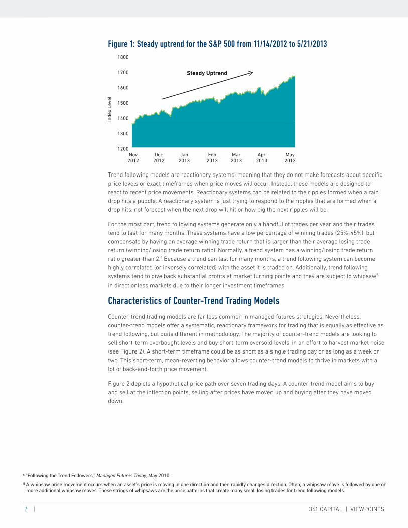
Figure 1 illustrates an ideal trading opportunity for a trend following system in the S&P 500®. In November 2012 the S&P 500 Index broke out into a 6-month uptrend gaining 24.55% in total return. This environment did not have many sharp reversals or a lot of back-

and-forth price movement, making for an easily identifiable uptrend.

Aditya Bhave Portfolio Manager, Managed Futures

Counter-Trend TradingA Systematic Method for Harvesting Short-Term Market Noise

The managed futures corner of the alternative investment space is one of the first places astute investors turn when they are seeking diversification from traditional asset classes.

1 “The Potential Role of Managed Commodity-Financial Futures Accounts (and/or Funds) in Portfolios of Stocks and Bonds,” Dr. John Lintner

2 We have chosen to focus on equities in this paper because our research indicates that equity markets are some of the most viable markets for short-term counter-trend trading. We believe this is largely due to the structure of equity markets and how they are traded, but this is an area that requires further research and exploration. Furthermore, our focus on equity markets does not imply counter-trend trading does not work on other asset classes. Other assets classes simply remain a frontier for further exploration.

3 “Frequently Asked Questions About Managed Futures,” www.cmegroup.com/education.

2 | 361 CAPITAL | VIEWPOINTS

Figure 1: Steady uptrend for the S&P 500 from 11/14/2012 to 5/21/2013

Trend following models are reactionary systems; meaning that they do not make forecasts about specific price levels or exact timeframes when price moves will occur. Instead, these models are designed to react to recent price movements. Reactionary systems can be related to the ripples formed when a rain drop hits a puddle. A reactionary system is just trying to respond to the ripples that are formed when a drop hits, not forecast when the next drop will hit or how big the next ripples will be.

For the most part, trend following systems generate only a handful of trades per year and their trades tend to last for many months. These systems have a low percentage of winning trades (25%-45%), but compensate by having an average winning trade return that is larger than their average losing trade return (winning/losing trade return ratio). Normally, a trend system has a winning/losing trade return ratio greater than 2.4 Because a trend can last for many months, a trend following system can become highly correlated (or inversely correlated) with the asset it is traded on. Additionally, trend following systems tend to give back substantial profits at market turning points and they are subject to whipsaw5

in directionless markets due to their longer investment timeframes.

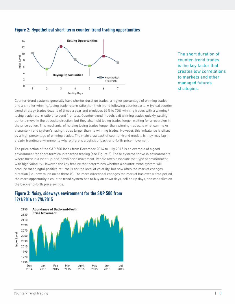
Characteristics of Counter-Trend Trading ModelsCounter-trend trading models are far less common in managed futures strategies. Nevertheless, counter-trend models offer a systematic, reactionary framework for trading that is equally as effective as trend following, but quite different in methodology. The majority of counter-trend models are looking to sell short-term overbought levels and buy short-term oversold levels, in an effort to harvest market noise (see Figure 2). A short-term timeframe could be as short as a single trading day or as long as a week or two. This short-term, mean-reverting behavior allows counter-trend models to thrive in markets with a lot of back-and-forth price movement.

Figure 2 depicts a hypothetical price path over seven trading days. A counter-trend model aims to buy and sell at the inflection points, selling after prices have moved up and buying after they have moved down.

4 “Following the Trend Followers,” Managed Futures Today, May 2010.

5 A whipsaw price movement occurs when an asset’s price is moving in one direction and then rapidly changes direction. Often, a whipsaw move is followed by one or more additional whipsaw moves. These strings of whipsaws are the price patterns that create many small losing trades for trend following models.

Inde

x Le

vel

1200

1300

1400

1500

1600

1700

1800

May2013

Apr2013

Mar2013

Feb2013

Jan2013

Dec2012

Nov2012

Steady Uptrend

Counter-Trend Trading | 3

Figure 2: Hypothetical short-term counter-trend trading opportunities

Counter-trend systems generally have shorter duration trades, a higher percentage of winning trades and a smaller winning/losing trade return ratio than their trend following counterparts. A typical counter-trend strategy trades dozens of times a year and produces 55% to 70% winning trades with a winning/losing trade return ratio of around 1 or less. Counter-trend models exit winning trades quickly, setting up for a move in the opposite direction, but they also hold losing trades longer waiting for a reversion in the price action. This mechanic, of holding losing trades longer than winning trades, is what can make a counter-trend system’s losing trades larger than its winning trades. However, this imbalance is offset by a high percentage of winning trades. The main drawback of counter-trend models is they may lag in steady, trending environments where there is a deficit of back-and-forth price movement.

The price action of the S&P 500 Index from December 2014 to July 2015 is an example of a good environment for short-term counter-trend trading (see Figure 3). These systems thrive in environments where there is a lot of up-and-down price movement. People often associate that type of environment with high volatility. However, the key feature that determines whether a counter-trend system will produce meaningful positive returns is not the level of volatility, but how often the market changes direction (i.e., how much noise there is). The more directional changes the market has over a time period, the more opportunity a counter-trend system has to buy on down days, sell on up days, and capitalize on

the back-and-forth price swings.

Figure 3: Noisy, sideways environment for the S&P 500 from 12/1/2014 to 7/8/2015

Inde

x Le

vel

0

2

4

6

8

10

12

14

7654321

Trading Days

HypotheticalPrice Path

Buying Opportunities

Selling Opportunities

Inde

x Le

vel

1950

1970

1990

2010

2030

2050

2070

2090

2110

2130

2150

Jul2015

Jun2015

May2015

April2015

Mar2015

Feb2015

Jan2015

Dec2014

Abundance of Back-and-Forth Price Movement

The short duration of counter-trend trades is the key factor that creates low correlations to markets and other managed futures strategies.

4 | 361 CAPITAL | VIEWPOINTS

An important point is that counter-trend models perform best when there is an abundance of back-and-forth price movement. This type of price movement can occur when volatility is low (daily price changes are smaller) or when volatility is high (daily price changes are larger). When volatility is high, the return potential for counter-trend models is amplified because price changes are larger and therefore winning trades are larger. On the flip side, the risk of drawdown also increases with volatility, and counter-trend models usually incur their biggest drawdowns in high volatility environments.

Finally, unlike trend following systems which can have sustained periods of high positive or negative correlation to the markets they are traded on, short-term counter-trend models typically have consistently low correlations to markets they are traded on. Counter-trend models take many short duration trades, both long and short, which allows the directionality of these positions to net out

fairly quickly.

Does Counter-Trend Trading Work?Counter-trend trading models are designed to identify short-term inflection points in the market. There is no universal definition for an inflection point, but they are often associated with instances when the market reaches a short-term extreme and then proceeds to revert from that extreme. To assess whether counter-trend trading works, we need to quantify short-term extremes and then test whether prices tend to revert at these extremes often enough to make counter-trend trading worthwhile. We can use 10-day highs and 10-day lows as a very simple proxy for short-term extremes.

To gauge the efficacy of trading counter to these short-term extremes, the S&P 500 was evaluated over 20 years, from the beginning of 1996 to the end of 2015, using a simple counter-trend model. If the S&P 500 made a new 10-day high, the counter-trend model went SHORT on the close and held the position until the next trading day’s close, betting against the upward momentum of the market. Conversely, if the S&P 500 made a new 10-day low, the counter-trend model went LONG on the close and held the position until the next trading day’s close, betting against the downward momentum of the market. Table 1 summarizes the results. Keep in mind that over this time period the S&P 500 had an annualized return

of 8.17% and an annualized volatility of 19.58%.

Table 1: 10-day high/low counter-trend model on the S&P 500 from 1/1/1996 to 12/31/2015

1996–2015 S&P 50010-DAY

HIGH/LOW MODEL

# Trades — 1,015

% Invested — 37.19%

Annualized Return 8.17% 9.89%

Annualized Std. Dev. 19.58% 11.96%

% Winning Trades — 68.97%

Winning/Losing Trade Return Ratio

— 0.71

The results in Table 1 show that trading counter to the S&P 500’s short-term market extremes was a viable strategy. The 10-day high/low counter-trend model took 1,015 trades and correctly identified an inflection point almost 70% of the time (68.97% winning trades). Furthermore, this simple counter-trend strategy outperformed the S&P 500 Index (9.89% v. 8.17% annualized return) even though it was only invested 37% of the time. The reduced investment level of the model is a large reason why its volatility

was about 60% of the S&P 500’s volatility over the same period (11.96% v. 19.58%).

Counter-Trend Trading | 5

To further explore the robustness of this simple counter-trend approach, new market highs and lows were measured using a range of periods from 5 to 15 days (see Figure 4). Over all of these periods, the high/low counter-trend model produced a positive annualized return, with an average annualized return of 8.71%. This level of consistency across different time periods strongly suggests that short-term counter-trend

trading has worked on the S&P 500 Index from 1996 to 2015.

Figure 4: Performance of counter-trend model over different rolling high/low periods

Trading counter-trend over the short run has worked on the S&P 500, but what about other markets? Table 2 summarizes the results of applying the simple, 10-day high/low counter-trend strategy to the EURO

STOXX 50 and the Nikkei 225 indices over the same timeframe.

Table 2: 10-day high/low counter-trend model on the S&P 500, EURO STOXX 50, and Nikkei 225 from 1/1/1996 to 12/31/2015

1996–2015S&P 500

MODEL

EURO STOXX  50

MODELNIKKEI 225

MODEL

# Trades 1,015 1,012 953

% Invested 37.19% 37.47% 37.28%

Annualized Return 9.89% 5.76% 0.95%

Annualized Std. Dev. 11.96% 13.82% 14.35%

% Winning Trades 68.97% 67.29% 66.11%

Winning/Losing Trade Return Ratio

0.71 0.61 0.54

Table 2 shows that the counter-trend model had a fairly similar signature when traded on the EURO STOXX 50 and the Nikkei 225, although the annualized return for the Nikkei 225 was not nearly as noteworthy as the other two indices.6 However, it is clear that the 10-day high/low model was able to produce a high percentage of winning trades in all three markets, confirming that short-term market extremes tend to revert more often than not.

Ann

ualiz

ed R

etur

n (%

)

0

2

4

6

8

10

12%

15141312111098765

Rolling High/Low Period (Trading Days)

8.71% Average Annualized Return

6 If you evaluate the performance of Nikkei 225’s 10-day high/low model, there are a few time periods that were especially ill-suited for counter-trend trading which explains most of the model’s underperformance. Specifically, the Nikkei 225 experienced unusually low levels of back-and-forth price movement (noise) in 2005 when that market went through a very strong uptrend. 2007 and 2010 both had pockets of abnormally low noise and 2012 was another year that had three strong trends resulting in extremely low levels of noise. These environments created several large losing trades for the 10-day high/low model, dragging down the model’s winning/losing trade return ratio and greatly dampening the model’s return. These extreme levels of low noise were isolated events, not found in other major world markets.

6 | 361 CAPITAL | VIEWPOINTS

The above results are impressive, especially when considering the simplicity of the counter-trend model that was used. Of course, transaction costs and slippage were not taken into account and the definitions of “short-term,” “overbought” and “oversold” were arbitrary. Nevertheless, the evidence supports the theory of short-term counter-trend trading holding up across several markets and across an extended

timeframe that included bull, bear, high volatility, and low volatility markets.

Why Does Counter-Trend Trading Work?A case has been made for the efficacy of counter-trend trading, but the real question is why does a counter-trend approach work? The simplest answer is that day-to-day market movements are dominated by noise. Over the short run, market participants are focused on their own investment timeframes and mandates. This includes managing operational functions, making decisions on how to allocate capital in and outside of the financial markets, and adhering to predefined investment rules. These peripheral agendas often do not align with the goal of maximizing returns and are therefore a major source of noise in the markets. For example, an investment fund may receive a redemption request, requiring the portfolio manager to liquidate a piece of the portfolio. The portfolio manager is not selling because these equities have reached fair value; instead, they are selling to meet an operational outflow, thereby injecting noise into the market and potentially driving prices away from fair value. At the same time, a large institution might be conducting a systematic rebalance, moving assets into the market simply because it’s the end of the quarter. It is these types of behaviors that contribute to the daily back-and-forth price movements that counter-trend models seek to exploit.

News events are also a rich source of noise. Markets react very quickly to news events, but they do not instantaneously arrive at a new theoretical price that perfectly accounts for the information in a news event. Instead, prices tend to swing back-and-forth until the new theoretical price is found. Figure 5 is a visualization of this process. If a negative news event is released, we would expect a perfectly efficient market to immediately find and move down to the new theoretical price. Then we would expect prices to remain static until another event changes the theoretical price again. This perfect reaction is illustrated by the “Efficient Price Path” in Figure 5. In reality, markets react to news events with a lot more noise,

creating price swings like those depicted by the “Hypothetical Price Path” in Figure 5.

Figure 5: Efficient price path v. Hypothetical price path

Why Counter-Trend Trading Works: The Importance of NoiseUp to this point, market noise has been cited repeatedly as being a primary reason why counter-trend models work; but “noise” has not been clearly defined. Market noise can be thought of simply as back-and-forth price movement. One way to quantify noise is by looking at the ratio of directional movement

Inde

x Le

vel

0

2

4

6

8

10

12

14

7654321

Hypothetical Price Path

E�cient Price Path

Trading Days

NegativeNews Event

Trading OpportunitiesBecause of Noise

Instantaneous Movement we would expect if Perfectly E�cient

Counter-Trend Trading | 7

7 “The Short-Term Counter-Trend Trading Strategy Guide,” Aditya Bhave and Nick Libertini

to total movement of a price path over a given time period. For example, if the S&P 500 gained 10 points every day for 10 days, the ratio of directional movement to total movement would be equal to 1.00 (100/100), because 100% of the Index’s daily movements were in the same direction. On the other hand, if the Index followed a noisier path like: [+50, -5, -35, +5, +45, +15, -25, +25, +35, -10] this ratio would equal 0.40 (100/250) indicating that only 40% of the Index’s total movement was directional (see Figure 6). One minus this ratio of directional movement to total movement produces the noise statistic (see Equation 1). In Figure 6, 60% of the movements would be considered noise for the “Noisy Price Path.” A noise statistic

closer to 0 indicates a less noisy market, while a statistic closer to 1 indicates a noise-rich market.

Figure 6: Noise-free price path v. Noisy price path

Equation 1: Noise statistic

N = # of trading days

N

Directional Movement = ∑ Price Change[i] i =1

N

Total Movement = ∑ ABS(Price Change[i]) i =1

Noise Statistic = 1– ABS(Directional Movement)

Total Movement

When we measure 20-day noise (monthly noise) on equity markets around the globe, the vast majority of observations are between 65% and 95%.7 So although 65% may seem like a high level of noise, it is actually on the low end of what we would expect to see. Noise levels between 75% and 85% are much more likely observations.

Using Equation 1 to quantify short-term market noise, a formal link can be established between the performance of short-term counter-trend trading and the level of market noise. To create this formal link we can use a large batch of random market data to isolate the interaction between market noise and the performance of the simple 10-day high/low counter-trend model. The benefit of using random market data is that you can generate thousands of different price paths, each having its own level of noise. Because there are so many price paths, the idiosyncrasies of any one path are washed out, allowing you to focus solely on the average relationship between the performance of the counter-trend model and noise. The large amount of different price paths also allows you to analyze the variation in counter-trend performance you could expect to see at any particular level of noise. This analysis can be done on real data, but because you only have one price path, it is more difficult to isolate the effect of noise on counter-trend performance.

Inde

x Le

vel

Trading Days

Noisy Price Path

Noise-Free Price Path

0

20

40

60

80

100

120

10987654321

8 | 361 CAPITAL | VIEWPOINTS

ftFor this analysis 10,000 random price paths were generated, each 10 years long, targeting a 0% expected return8 and an annualized volatility of 15%. The paths were generated by randomly drawing daily returns from a normal distribution,9 thus creating a large batch of 10 year “random walks.” The average 20-day noise was calculated for each of the 10-year price paths. Then the simple 10-day high/low counter-trend model was run on each price path, and the model’s annualized performance was calculated. Figure 7 shows the strong linear relationship between noise and the counter-trend model’s annualized return. The correlation between average 20-day noise of the random 10-year price paths and the annualized return of the 10-day high/low counter-trend model run on those price paths was 62.18%, resulting in a percent of variance explained of 38.66%. Figure 8 shows the average model return and

range of model returns for the most common noise levels observed in the batch of random price paths.

Figure 7: Relationship between average 20-day noise and 10-day high/low counter-trend model performance

Figure 8: Average, max, and min annualized return of 10-day high/low counter-trend model at common noise levels

Figures 7 and 8 show that the performance of short-term counter-trend trading depends heavily on the noise level of the market. The higher the noise level, the better chance the model has of producing a positive return. The analysis also reveals that a high level of noise does not guarantee a positive return.

Ann

ualiz

ed M

odel

Ret

urn

(%)

Average 20-Day Noise

73% 74% 75% 76% 77% 78% 79% 80% 81% 82%-10

-8

-6

-4

-2

0

2

4

6

8

10% R2 = 38.66%

8 0% expected return was chosen so there was no directional bias imparted to the price paths. However, the findings using varying levels of positive and negative expected return are consistent with the findings using 0% expected return. Using non-zero levels of expected return simply reduces the diversity of noise levels within the sample of price paths and it would create a divergence in the expectations of long trades v. short trades depending on the sign of the bias.

9 For simplicity, we used a normal distribution even though equity returns are not normally distributed. The findings using an empirical distribution composed of real equity returns are consistent with the findings using a normal distribution.

Ave

rage

Ann

ualiz

ed M

odel

Ret

urn

(%)

But PositiveReturns arenot Guaranteedat High Levelsof Noise

75% 76% 77% 78% 79% 80% 81%

-15

-10

-5

0

5

10

15%

Average 20-Day Noise

Performance Increaseswith Noise

Counter-Trend Trading | 9

Looking at Figure 8, we can see that even when the average noise level was above 80%, the 10-day high/low counter-trend model still produced a negative return over some of the price paths. These conclusions were made by examining a large batch of random price paths, so we can be fairly confident in the relationship between noise and counter-trend performance.

Revisiting the three markets the 10-day high/low counter-trend model was tested on (the S&P 500, the EURO STOXX 50, and the Nikkei 225), we can see, in Table 3, that each market’s average 20-day noise was also correlated with the yearly performance of the 10-day high/low model. The relationship is not as consistent as the one observed using random market data, but this is largely due to the finite amount of real market data, with each market representing only one price path. Even still, we can see that in the real

market data, noise is a major driver of short-term counter-trend performance.

Table 3: Annual correlation of the 10-day high/low counter-trend model to the average 20-day noise

S&P 500 MODEL

EURO STOXX  50

MODELNIKKEI 225

MODEL

Correlation 20-day Noise

50.37% 68.49% 31.43%

Will Counter-Trend Models Continue to Work?The biggest pushback against quantitative trading models is the belief that “models always break.” Therefore it seems prudent to address the question of whether short-term counter-trend models will continue to produce returns like those realized by the 10-day high/low model from 1996 to 2015. Based on the previous section, it is apparent that the noise level of market movements is the governing factor of whether a short-term counter-trend approach is viable. To address the question of whether short-term counter-trend models will continue to work, we really need to ask whether the noise level of the market will be high enough to make counter-trend trading worthwhile.

Figure 9 depicts the trend of noise in the S&P 500 and the performance of the 10-day high/low counter-trend model over the 46 years from 1970 to 2015. It is apparent from Figure 9 that noise has increased consistently from the low 70%’s to the high 70%’s and the counter-trend model’s performance has improved almost in lock-step with this rise. We can see that around the mid to late 1990’s the noise level reached a point where the 10-day high/low model was profitable to trade, and the average level of noise has remained above this threshold ever since.

Figure 9: Trend of average 20-day noise and the annualized return of the 10-day high/low counter-trend model on the S&P 500 from 1970 to 2015

10yr

Ave

rage

of 2

0-D

ay N

oise

10 Y

ear

Ann

ualiz

ed P

erfo

rman

ce (%

)

70

72

74

76

78

80%

20142009200419991994198919841979

Rolling 10yr Avg 20d Noise

Rolling 10yr Model Return

Linear (Rolling 10yr Avg 20d Noise)-20

-15

-10

-5

0

5

10

15

20

25%

10 | 361 CAPITAL | VIEWPOINTS

It seems that the current noise level is high enough to make counter-trend trading viable, but will market noise remain elevated going forward? To try to answer this question we need to understand what caused noise to rise in the first place and what has kept the level of noise elevated. As discussed earlier, noise is a byproduct of markets not reacting efficiently to news events over the short-term and market participants carrying out their independent agendas that may not align perfectly with the goal of maximizing total return. Therefore, the level of market noise is dependent on the ability of market participants to express their opinions by trading. The easier it is to trade, the more rapidly opinions can be expressed. The more rapidly opinions can be expressed, the more noise there will be in market movements. Conversely, if market liquidity is low, if trading costs are high, or if news is sparse there will be less activity in the market and therefore lower noise on average.

Referring back to Figure 9, we know that there were several noteworthy structural shifts in the way the S&P 500, and equity markets in general, were traded from 1970 to 2015. Over that time period, equity markets realized a massive influx of liquidity due in large part to the introduction of electronic trading, the rolling out of many different equity futures products, the introduction of exchange traded funds (ETFs), and the steady decline of broker fees for trading. Additionally, there were several changes made to the way stocks were priced. Prices were changed from being quoted in one-eighth increments to one-sixteenths and then they were eventually changed to being quoted in decimals. This had a very significant impact on the bid/ask spread of most stocks, making equities cheaper to trade. All of these changes contributed to making equities easier and cheaper to trade, and are likely the major reason we have seen such a notable increase in noise from 1970 onward.

All of the structural changes cited have an intuitive link to activity levels of market participants.

What is perhaps less concrete is the link between activity and noise. It makes sense that the more often market participants trade, the more noise there will be in price movements; but, it would be nice to have a simple model that could confirm the relationship between activity level and noise.

To examine this relationship between activity level and noise, we considered a very simple hypothetical market consisting of 1,000 market participants trading daily over the course of one year. Each participant controlled 1 share of stock and made their decision to buy or sell that share randomly. The only parameter in the model was how often each participant made a decision to buy or sell. A high parameter value would result in the market participants buying and selling frequently, maybe even every day. A low parameter value would result in market participants buying and selling infrequently, maybe only a few times a year. We varied the activity parameter from low to high to see how the average activity level of the participants affected the noise of this simple market. We looked at this analysis over 1,000 simulations to ensure that the idiosyncrasies of any one simulated year were washed out. The results are

summarized in Figure 10.

Figure 10: Impact of average activity level on the average 20-day noise of a simple market

Ave

rage

20-

day

Noi

se (%

)

50

60

70

80

90

100%

Low Trading Activity High Trading Activity

Average Activity Level

If trading is cheaper and easier, people will trade more. If trading is more expensive, or if market access is more difficult, people will trade less.

Counter-Trend Trading | 11

From Figure 10, we can see that there is a clear link between the average activity level of market participants and the average 20-day noise of the market. The higher the activity level, the higher the noise. Of course, this was a very simple representation of the activity in a real market. Real markets are extremely complex and perfectly modeling all the interactions would be an impossible task. Nonetheless, this simple model confirms our intuition that there is probably a link between the activity level of market participants and the level of noise in a market’s price movements.

Clearly, there have been several key structural shifts from 1970 to 2015 that had a meaningful impact on the activity level of market participants. Our simple model highlights that higher activity levels lead to more noise, which is the main reason why it has been profitable to trade against short-term price extremes from 1996 to 2015. This shift to higher levels of noise does not imply that markets no longer trend; instead, it indicates that there is enough back-and-forth price action in market movements to make counter-trend trading viable. If liquidity abates and transaction costs revert to much higher levels, then market noise may subside again, reducing the potency of short-term counter-trend models. However, human psychology is relatively static, which means that trading decisions that give rise to noise are not going to disappear, as long as humans are making financial decisions. Likewise, technology is going to progress in the future, further reducing transaction costs and the availability of information. This should sustain the heightened level of noise and allow counter-trend models to flourish.

ConclusionCounter-trend models offer a systematic method for exploiting back-and-forth price swings and they have consistently low correlation to traditional asset classes and other managed future strategies. The performance expectation of short-term counter-trend models is fundamentally linked to the level of market noise; the more back-and-forth price swings, the higher the market noise, the better the counter-trend performance. Higher noise is a byproduct of increased trading activity, which has risen in response to increases in liquidity, decreases in transaction costs, and increases in the flow of news.

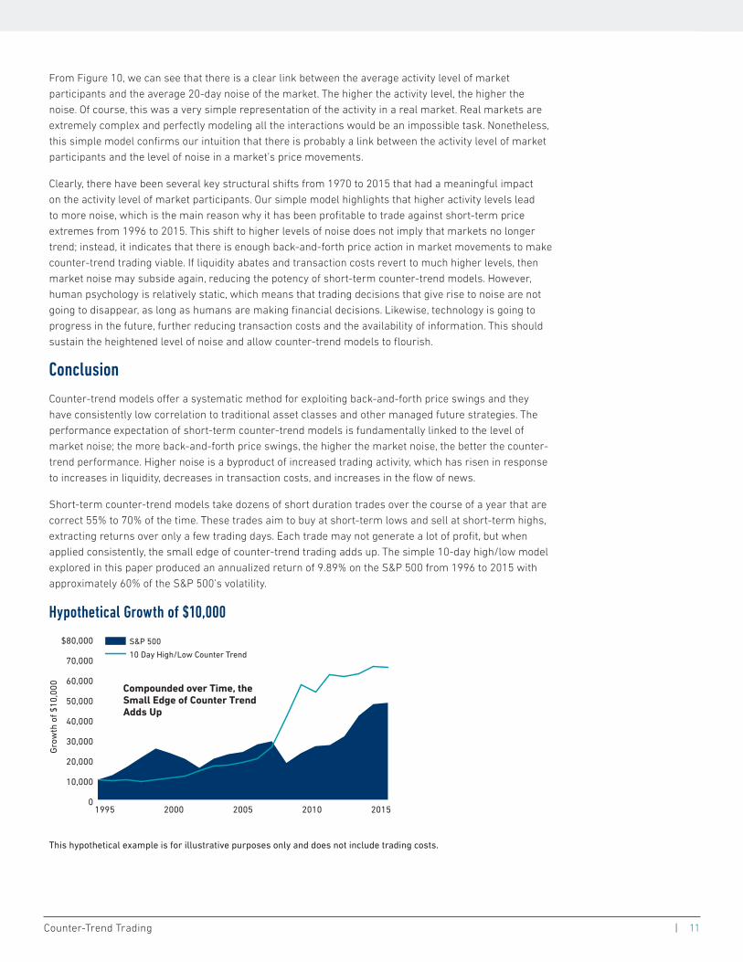
Short-term counter-trend models take dozens of short duration trades over the course of a year that are correct 55% to 70% of the time. These trades aim to buy at short-term lows and sell at short-term highs, extracting returns over only a few trading days. Each trade may not generate a lot of profit, but when applied consistently, the small edge of counter-trend trading adds up. The simple 10-day high/low model explored in this paper produced an annualized return of 9.89% on the S&P 500 from 1996 to 2015 with approximately 60% of the S&P 500’s volatility.

Hypothetical Growth of $10,000

This hypothetical example is for illustrative purposes only and does not include trading costs.

Gro

wth

of $

10,0

00 Compounded over Time, the Small Edge of Counter TrendAdds Up

0

10,000

20,000

30,000

40,000

50,000

60,000

70,000

$80,000

20152010200520001995

S&P 500

10 Day High/Low Counter Trend

However, counter-trend models tend to lag in strong trending environments due to the lack of back-and-forth price swings. These models are also susceptible to a structural decrease in market noise. Should a catalyst arise that would meaningfully reduce the amount of trading activity in equity markets it would be reasonable to expect short-term counter-trend models to be rendered unviable. Still, counter-trend models should remain to be a worthwhile source of low correlation returns over the foreseeable future due to technological and industry trends that continuously make trading cheaper and easier.

For more viewpoints: Call 866.361.1720 or visit 361capital.com.

361 Capital | 4600 South Syracuse Street, Suite 500, Denver, CO 80237 | 866.361.1720 | 361capital.com | Follow us on LinkedIn and Twitter:

The opinions are those of the 361 Capital Investment Team, as of January 2016 and are subject to change at any time due to changes in market or economic conditions. The comments should not be construed as a recommendation of individual holdings or market sectors, but as an illustration of broader themes. 361 Capital makes no representation as to whether any illustration/example mentioned in this document is now or was ever held in any products advised by 361 Capital. Past performance is not indicative of future results. Illustrations are only for the limited purpose of analyzing general market or economic conditions and demonstrating 361 Capital’s research process. In preparing this document, 361 Capital has relied upon and assumed, without independent verification, the accuracy and completeness of all information available from public sources.

This 361 Capital article is not intended to provide investment advice. This paper should not be construed as an offer to sell, a solicitation of an offer to buy, or a recommendation for any security by 361 Capital or any third-party. You are solely responsible for determining whether any investment, investment strategy, security or related transaction is appropriate for you based on your personal investment objectives, financial circumstances and risk tolerance. You should consult your legal or tax professional regarding your specific situation.

About 361 Capital361 Capital is a leading boutique asset manager focused on alternative and behavioral-based equity solutions that seek to deliver meaningful alpha, manage risk and offer diversification potential to investor portfolios. Founded in 2001, we offer a suite of investment products including Long/Short Equity, Managed Futures, Macro, as well as Small, Mid and Large Cap Equity.