trading and information di usion in over-the-counter...
TRANSCRIPT
Trading and Information Diffusion in Over-the-Counter Markets∗
Ana Babus
Washington University in St. Louis
Peter Kondor
London School of Economics
April 12, 2018
Abstract
We propose a model of trade in over-the-counter (OTC) markets in which each dealer with
private information can engage in bilateral transactions with other dealers, as determined by
her links in a network. Each dealer’s strategy is represented as a quantity-price schedule. We
analyze the effect of trade decentralization and adverse selection on information diffusion,
expected profits, trading costs and welfare. Information diffusion through prices is not
affected by dealers’ strategic trading motives, and there is an informational externality
that constrains the informativeness of prices. Trade decentralization can both increase or
decrease welfare. A dealer’s trading cost is driven by both her own and her counterparties’
centrality. Central dealers tend to learn more, trade more at lower costs and earn higher
expected profit.
JEL Classifications: G14, D82, D85
Keywords: information aggregation; bilateral trading; demand schedule equilibrium; tra-
ding networks.
∗Email addresses: [email protected], [email protected]. We are grateful to Andrea Eisfeldt, BernardHerskovic, Burton Hollifield, Alejandro Justiniano, Leonid Kogan, Semyon Malamud, Gustavo Manzo, ArtemNeklyudov, Marzena Rostek, Chester Spatt, Alireza Tahbaz-Salehi, Pierre-Olivier Weill, the editor, the anony-mous referees and numerous seminar participants. Peter Kondor acknowledges the financial support of the PaulWoolley Centre at the LSE and the European Research Council (Starting Grant #336585).
1
1 Introduction
A vast proportion of financial assets is traded in over-the-counter (OTC) markets. In these
markets, transactions are bilateral, prices are dispersed, trading relationships are persistent,
and typically, a few large dealers intermediate a large share of the trading volume. In this
paper, we explore a novel approach to modeling OTC markets that reflects these features.
In our model, each dealer with private information can engage in several bilateral transacti-
ons with her potential trading partners, as determined by her links in a network. Each dealer’s
strategy is represented as a quantity-price schedule. Our focus is on how decentralization
(characterized by the structure of the dealer network) and adverse selection jointly influence
information diffusion, expected profits, trading costs, and welfare. We prove that information
diffusion through prices is not affected by strategic considerations in a well-defined sense. We
show that each equilibrium price depends on all the information available in the economy,
incorporating even the signals of dealers located far from a given transaction. We identify
an informational externality that constrains the informativeness of prices. We highlight that
decentralization can both increase or decrease welfare and that an important determinant of a
dealer’s trading cost besides her own centrality is the centrality of her counterparties. Using an
example calibrated to securitization markets, we argue that in realistic interdealer networks,
more central dealers learn more, trade more at lower costs, and earn higher expected profit.
However, we also explain why in some special cases, more-connected dealers can earn a lower
expected profit.
In our main specification, there are n risk-neutral dealers organized in a dealer network.
Intuitively, a link between i and j indicates that they are potential counterparties in a trade.
There is a single risky asset in zero net supply. The final value of the asset is uncertain and
interdependent across dealers, with an arbitrary correlation coefficient controlling the relative
importance of the common and private components. Each dealer observes a private signal
about her value, and all dealers have the same quality of information. Since the values are
interdependent, it is valuable to infer each other’s signals. Values and signals are drawn from
a known multivariate normal distribution. Each dealer simultaneously chooses her trading
strategy, understanding her price effect given other dealers’ strategies. For any private signal,
each dealer’s trading strategy is a generalized demand function that specifies the quantity of
2
the asset she is willing to trade with each of her counterparties, depending on the vector of
prices in the transactions in which she engages. Each dealer, in addition to trading with other
dealers, trades with price-sensitive customers. In equilibrium, prices and quantities must be
consistent with the set of generalized demand functions and the market clearing conditions
for each link. We refer to this structure as the OTC game. The OTC game is, essentially,
a generalization of the Vives (2011) variant of Kyle (1989) to networks. We consider general
connected networks.
We show that the equilibrium beliefs in the OTC game are independent of dealers’ strategic
considerations. In fact, we construct a separate game, in which dealers do not trade, that
generates the same posterior beliefs. In this simpler, auxiliary game, dealers are connected
in the same network and act in the same informational environment as in the OTC game.
However, the dealers’ aim is to make a best guess of their own value conditional on their
signals and the guesses of the other dealers to which they are connected. We refer to this
structure as the conditional guessing game. Because each dealer’s equilibrium guess depends
on her neighbors’ guesses, and through those, on her neighbors’ neighbors’ guesses, etc., each
equilibrium guess partially incorporates the private information of all the dealers in a connected
network. However, dealers do not internalize how the informativeness of their guess affects
others’ decisions, and the equilibrium is typically not informationally efficient. That is, dealers
tend to put too much weight on their own signal, thereby making their guess inefficiently
informative about the common component.
In the OTC game, we show that each equilibrium price is a weighted sum of the posterior
beliefs of the counterparties that participate in the transaction; hence, it inherits the main
properties of the beliefs. In addition, each dealer’s equilibrium position is proportional to the
difference between her expectation and the price. Therefore, a dealer tends to sell at a price
higher than her belief to relatively optimistic counterparties and buys at a price lower than her
belief from pessimists. This results in dispersed prices and profitable intermediation for dealers
with many counterparties, as is characteristic of real-world OTC markets. The proportionality
coefficient of a dealer’s position is the inverse of her price impact in that transaction. In turn,
the dealer’s price impact is smaller if her counterparty is less concerned about adverse selection,
either because the common value component is less important or because she is more central
and learns from several other prices.
3

To gain further insights into our main topics, we proceed in two distinct ways. First, using
a network associated with the securitization market as presented by Hollifield et al. (2016) we
show that more-connected dealers learn more, intermediate more, trade a larger gross volume
with a lower price impact, and make more profit. We also illustrate how our parameters can be
matched to the data and contrast our predictions with the findings from the empirical literature
across various markets.
Second, we gain further insights into welfare, expected profits, and illiquidity by analyzing
trade in various simple networks. In particular, we isolate the effect of decentralization by
comparing the complete OTC network with centralized markets; we illustrate the role of link
density by comparing circulant OTC networks in which we successively increase the number
of links that each dealer has, and we analyze the effect of asymmetric number of links in the
star OTC network. We show that centralized trading might not improve welfare and explain
that for certain parameters, more links imply more profits only when the network exhibits
assortativity.
Finally, we argue that our one-shot game can be interpreted as a reduced form of the
complex dynamic bargaining process that leads to price determination in real-world OTC
markets by constructing an explicit, decentralized protocol for the price-discovery process.
This exercise also highlights the advantages and limitations of our static approach compared
to a full dynamic treatment.
Related literature
Most models of OTC markets are based on search and bargaining (e.g., Duffie et al. (2005);
Duffie et al. (2007); Lagos et al. (2008); Vayanos and Weill (2008); Lagos and Rocheteau
(2009); Afonso and Lagos (2012); and Atkeson et al. (2012)). By construction, in search
models, transactions are between atomistic dealers through non-persistent links. Therefore,
our approach is more suitable for capturing the effects of high market concentration implied
by the presence of few large dealers intermediating the bulk of the trading volume. At the
same time, we collapse trade to a single period, thus missing implications of the dynamic
dimension. In this sense, we view these approaches to be complementary. However, models
of learning through trade based on search require non-standard structures and are difficult to
compare to existing results regarding centralized markets (e.g., Duffie et al. (2009); Golosov
4
et al. (2009)).1 Our approach is compatible with the standard, jointly normal framework of
asymmetric information and learning.
There is a growing literature studying trading in a network (e.g., Kranton and Minehart
(2001); Rahi and Zigrand (2006); Gale and Kariv (2007); Gofman (2011); Condorelli and
Galeotti (2012); Choi et al. (2013); Malamud and Rostek (2013); Manea (2013); Nava (2013)).
These papers typically consider either the sequential trade of a single unit of the asset or a
Cournot-type quantity competition.2 In contrast, we allow agents to form (generalized) demand
schedules conditioning the quantities for each of their transactions on the vector equilibrium
prices in these transactions. This emphasizes that the terms of the various transactions of
a dealer are interconnected in an OTC market. Additionally, to our knowledge, none of the
papers within this class addresses the issue of information aggregation which is the focus of
our analysis.3
A separate literature studies Bayesian (Acemoglu et al. (2011)) and non-Bayesian (Bala
and Goyal (1998); DeMarzo et al. (2003); Golub and Jackson (2010)) learning in the context
of arbitrary connected social networks. In these papers, agents update their beliefs about a
payoff-relevant state after observing the actions of their neighbors in the network. Our model
complements these works by considering that (Bayesian) learning occurs through trading.
The paper is organized as follows. The following section introduces the model set-up and the
equilibrium concept. In Section 3, we derive the equilibrium and give sufficient conditions for its
existence. We characterize the informational content of prices and characteristics of information
diffusion in Section 4. In Section 5, we study expected profit, welfare, and illiquidity based
on some of the most common networks and calibrate our model to securitization markets. In
Section 6, we show how our one-shot game can be interpreted as a reduced form of the complex
dynamic bargaining process. Finally, we conclude.
1The main focus of these models is the time-dimension of information diffusion across agents. In thesemodels, incentives to share information and to learn are driven by the fact that two agents meet repeatedly orany agent meets with counterparties of their counterparties with zero probability. This is in contrast with ourapproach, in which dealers understand that the network structure may lead to overlapping information amongtheir counterparties.
2As an exception, Malamud and Rostek (2013) also use a multi-unit double-auction set-up to model a decen-tralized market. However, they do not consider the problem of learning through trade.
3Whereas there is another stream of papers (e.g., Ozsoylev and Walden (2011); Colla and Mele (2010);Walden (2013)) that consider that traders have access to the information of their neighbors in a network, inthese models, trade takes place in a centralized market.
5

2 A General Model of Trading in OTC Markets
2.1 The model set-up
We consider an economy with n risk-neutral dealers that trade bilaterally a divisible risky
asset.4 All trades take place at the same time. Dealers, in addition to trading with each other,
also serve a price sensitive customer-base. Each dealer is uncertain about the value of the asset.
This uncertainty is captured by θi, referred to as dealer i’s value. We consider that values are
interdependent across dealers. In particular, the value of the asset for dealer i can be explained
by a component, θ, that is common to all dealers and a component, ηi, that is specific to dealer
i such that
θi = θ + ηi,
with θ ∼ N(0, σ2θ), ηi ∼ IIDN(0, σ2
η), and V(θ, ηi) = 0, where V (·, ·) represents the variance-
covariance operator. This implies that θi is normally distributed with mean 0 and variance
σ2θ = σ2
θ+ σ2
η. The common value component stands for the uncertain cash-flow from the
asset. The private value component is a short-cut for unmodeled differences in the utility a
dealer derives from this cash-flow, because of differences in background risk, in the usage of
the asset as collateral, in technologies to repackage and resell cash flows or in risk-management
constraints, for example. The degree of the interdependence between dealers’ values is captured
by the correlation coefficient
ρ =σ2θ
σ2θ
,
where ρ ∈ [0, 1]. This representation is useful because we can vary the degree of interdepen-
dence, ρ, while keeping the variance σ2θ constant.
The asset is in zero net supply. This is without loss of generality, provided supply is
constant. We do not assume any constraints on the sizes or signs of dealers’ positions.
We assume that each dealer receives a private signal, si, such that
si = θi + εi,
where εi ∼ IIDN(0, σ2ε) and V(θj , εi) = 0, for all i and j.
4While our paper focuses exclusively on over-the-counter markets, in online Appendix C we show how ourframework can be generalized to model other partially segmented markets.
6

Dealers are organized into a trading network, g. A link ij ∈ g implies that i and j are
potential trading partners, or neighbors in the network g. Intuitively, agent i and j know and
sufficiently trust each other to trade if they find mutually agreeable terms. Let gi denote the
set of i’s neighbors and mi ≡∣∣gi∣∣ the number of i’s neighbors. If two dealers have a link, let
qiij denote the quantity that dealer i trades over link ij. The price at which trade takes place
is denoted by pij . Links in the network are undirected, such that if ij ∈ g, then ji ∈ g also.
The notation reflects this property. For instance, pij = pji and qiij = qiji.
Whereas our main results hold for any network, throughout the paper, we illustrate the
results using two main types of networks as examples.
Example 1 In an (n,m) circulant network with n odd and m < n even, if dealers are
arranged in a ring then each dealer is connected with m/2 other dealers on her left and m/2 on
her right. The (n, 2) circulant network is the circle, whereas the (n, n− 1) circulant network is
the complete network.
Example 2 In a star network, one dealer is connected with n−1 other dealers, and no other
links exist.
We define a one-shot game in which each dealer chooses an optimal trading strategy, provi-
ded she takes as given others’ strategies but she understands that her trade has a price effect.
In particular, the strategy of dealer i is a map from the signal space to the space of generalized
demand functions. For each dealer i with signal si, a generalized demand function is a conti-
nuous function Qi : Rmi → Rm
ithat maps the vector of prices5, pgi = (pij)j∈gi , that prevail
in the transactions that dealer i participates in network g into a vector of quantities she wishes
to trade with each of her counterparties. The j-th element of this correspondence, Qiij(si; pgi),
represents her demand function when her counterparty is dealer j, such that
Qi(si; pgi) =(Qiij(s
i; pgi))j∈gi
.
Note that a dealer can buy a given quantity at a given price from one counterparty and
sell a different quantity at a different price to another at the same time. When dealer i buys
5A vector is always considered to be a column vector unless explicitly stated otherwise.
7
on the link ij, the quantity qiij = Qiij(si; pgi) is positive. Conversely, when dealer i sells on the
link ij, the quantity qiij is negative.
The demand function of dealer i in a transaction with dealer j, Qiij(si; pgi), depends on
all the prices pgi . For example, if k is linked to i who is linked to j, a high demand from
dealer k might raise the bilateral price pki. This might make dealer i revise her estimate of
her value upwards and adjust her quantity supplied to both k and j accordingly. However,
Qiij(si; pgi) depends only on pgi , not on the full price vector. This emphasizes a critical feature
of OTC markets, namely, that the price and quantity traded in a bilateral transaction are
known only by the two counterparties involved in the trade and not immediately revealed to
all market participants. Whereas OTC trading protocols do not typically involve the submission
of full demand schedules, we think of generalized demand functions as a reduced-form price
determination mechanism that captures the repeated exchange of limit and market orders (i.e.,
the offer and acceptance of quotes) across fixed counterparties that have persistent links, within
a short time-interval. To illustrate this mapping, we explicitly model the price-discovery process
in Section 6. This also shows why our specification need not rely on the implicit assumption
of a Walrasian auctioneer.
Apart from trading with each other, each dealer also serves a price-sensitive customer base.
Customers have quadratic preferences for holding a quantity q of the asset. We assume that
a dealer i uses each link ij to satisfy an exogenously given fraction of her customer base. In
particular, we consider that dealer i trades with the customers she associates to the link ij at
the same price she trades with dealer j, pij , adjusted by an exogenous markup. This implies
that for each transaction between i and j, the customer base generates a downward-sloping
demand
Dij(pij) = βijpij , (1)
where the constant βij < 0 is a summary statistic for dealer i and j’s customers’ preferences
and the markup that the dealers charge.6 Just as the dealers do, customers in our model
take the network structure as given and do not search across dealers for better prices. This
specification captures in reduced form the fact that clients in OTC markets typically have very
6For example, suppose that the marginal utility of each customer buying quantity q is 1βq. If a customer is
associated to a link ij, she will pay pij (1 + µij) per unit where µij is the markup. Then, her inverse demandfunction is given by 1
βq = pij (1 + µij), that is βij = β (1 + µij).
8
few and long-lasting dealer relationships. For instance, Hendershott et al. (2016) document
that a large group of clients in the corporate bond market trade with a single dealer annually.
The expected payoff for dealer i corresponding to the strategy profile{Qi(si; pgi
)}i∈{1,...,n}
is
E
∑j∈gi
Qiij(si; pgi)
(θi − pij
)|si,pgi
, (2)
where pij are the elements of the bilateral clearing price vector p defined by the smallest element
of the set
P({
Qi(si; pgi
)}i, s)≡{
p∣∣∣ Qiij (si; pgi)+Qjij
(sj ; pgj
)+ βijpij = 0, ∀ ij ∈ g
}(3)
by lexicographical ordering7, if P is non-empty. While in equilibrium qiij and qjij tend to have
the opposite sign, qiij 6= −qjij , because the customers also trade a quantity βijpij . If P is empty,
we choose p to be the infinity vector and say that the market breaks down and define all
dealers’ payoff to be zero. We refer to the collection of rules that define a unique vector p
for any given realization of signals and strategy profile as P({
Qi(si; pgi
)}i, s). Introducing
the set (3) ensures that we can evaluate dealers’ payoffs for any demand functions that dealers
may choose. This will allow us to search for a Bayesian Nash equilibrium, as explained in the
following section.
2.2 Equilibrium concept
The environment described above represents a Bayesian game, henceforth referred to as the
OTC game. The risk-neutrality of dealers and the normal information structure allows us to
search for a linear equilibrium of this game, which is defined as follows.
Definition 1 A Linear Bayesian Nash equilibrium of the OTC game is a vector of linear
generalized demand functions{Q1(s1; pg1),Q2(s2; pg2), ...,Qn(sn; pgn)
}such that Qi(si; pgi)
7The specific algorithm we choose to select a unique price vector is immaterial. To ensure that our game iswell defined, we need to specify dealers’ payoffs as a function of strategy profiles both on and off the equilibriumpath.
9

solves the problem
max(Qiij)j∈gi
E
∑j∈gi
Qiij(si; pgi)
(θi − pij
) ∣∣si,pgi , (4)
for each dealer i, where p = P (·, s).
A dealer i chooses a demand function, Qiij (·), for each transaction ij, to maximize her
expected profits, given her information, si, and given the demand functions chosen by the
other dealers. Implicit in the definition of the equilibrium is that each dealer understands that
she has a price impact when trading with the counterparties given by the network g. Solving
problem (4) is equivalent to finding a fixed point in demand functions.
3 The Equilibrium
In this section, we derive the equilibrium in the OTC game. First, we derive the equilibrium
strategies as a function of posterior beliefs. Second, we construct posterior beliefs. Third,
we provide sufficient conditions for the existence of the equilibrium in the OTC game for any
network.
3.1 Derivation of demand functions
Our derivation follows Kyle (1989) and Vives (2011). We conjecture an equilibrium in linear
demand functions, such that the demand function of any given dealer i in the transaction with
a counterparty j is
Qiij(si; pgi) = tiij(y
iijs
i +∑k∈gi
ziij,ikpik − pij). (5)
We refer to tiij as the trading intensity of dealer i on the link ij, whereas yiij and ziij,ik capture
the effects specific to the dealer’s private signal and the price pik on the quantity that dealer
i demands on the link ij. As will become clear below, dealer i’s best response is (5) when all
other agents’ demand functions are given by (5).
As is standard in similar models, we simplify the optimization problem (4), which is defined
over a function space, to finding the functions Qiij(si; pgi) point-by-point. For this, we fix a
realization of the vector of signals, s. Then, we solve for the optimal quantity qiij that each
10

dealer i demands when trading with a counterparty j as she takes the demand functions of the
other dealers as given. Thus, we obtain dealer’s i best response quantity qiij in the transaction
with dealer j for each realization of the signals. This essentially gives us a map from prices to
quantities, or her demand function. We describe the procedure in detail below.
Given the conjecture (5) and market clearing
Qiij(si; pgi) +Qjij(s
j ; pgj ) + βijpij = 0, (6)
the residual inverse demand function of dealer i in a transaction with dealer j is
pij = −tjij(y
jijs
j +∑
k∈gj ,k 6=i zjij,jkpjk) + qiij
βij + tjij
(zjij,ij − 1
) . (7)
Denote
Ijij ≡ −tjij(y
jijs
j +∑
k∈gj ,k 6=i zjij,jkpjk)
βij + tiij
(zjij,ij − 1
) (8)
and rewrite (7) as
pij = Ijij −1
βij + tjij
(zjij,ij − 1
)qiij . (9)
The uncertainty that dealer i faces about the signals of others is reflected in the random
intercept of the residual inverse demand, Ijij , whereas her capacity to affect the price is reflected
in the slope −1/(βij + tjij
(zjij,ij − 1
)). Thus, the price pij is informationally equivalent to
the intercept Ijij . This implies that finding the vector of quantities qi = Qi(si; pgi) for one
particular realization of the signals, s, is equivalent to solving
max(qiij)j∈gi
∑j∈gi
qiij
E (θi|si,pgi)+1
βij + tjij
(zjij,ij − 1
)qiij − Ijij .
From the first-order conditions, we derive the quantities qiij for each link of i and for each
realization of s as
21
βij + tjij
(zjij,ij − 1
)qiij = Ijij − E(θi|si,pgi
).
Then, using (9), we can find the optimal demand function for each dealer i when trading with
11

dealer j:
Qiij(si; pgi) = −
(βij + tjij
(zjij,ij − 1
)) (E(θi
∣∣si,pgi )− pij) . (10)
Furthermore, given our conjecture (5), equating coefficients in equation (10) implies that
E(θi∣∣si,pgi ) = yiijs
i +∑k∈gi
ziij,ikpik.
However, the projection theorem implies that the belief of each dealer i can be described as
a unique linear combination of her signal and the prices she observes. Thus, it must be that
yiij = yi and ziij,ik = ziik for all i, j, and k. In other words, the posterior belief of a dealer i is
given by
E(θi|si,pgi
)= yisi + zgipgi , (11)
where zgi =(ziij
)j∈gi
is a row vector of size mi. Then, we obtain that the trading intensity of
dealer i is the inverse of her price impact in the transaction with dealer j, or
tiij = tjij
(1− zjij
)− βij . (12)
Substituting (11) back into our conjecture (5), we obtain that the demand of dealer i in a
transaction with dealer j is given by
Qiij(si; pgi) = tiij
(E(θi|si,pgi
)− pij
). (13)
That is, the quantity that dealer i trades with j is the perceived gain per unit of the asset,(E(θi|si,pgi
)− pij
), multiplied by the endogenous trading intensity parameter, tiij . Moreover,
by substituting the optimal demand function (13) into the bilateral market clearing condition
(6), we obtain the equilibrium price between any pair of dealers i and j as a linear combination
of the posterior beliefs of i and j:
pij =tiijE(θi
∣∣si,pgi ) + tjijE(θj∣∣si,pgj )
tiij + tjij − βij, (14)
At this point, we depart from the standard derivation. The standard approach is to deter-
mine the coefficients of the demand function (5) using a fixed-point argument. In particular,
12
given our conjecture (5), the bilateral clearing conditions represent a system of linear equati-
ons from which prices can be derived as an affine combination of signals. Then, the projection
theorem implies that for each dealer i, the coefficients yi and zgi must satisfy the following
fixed-point condition:
yi
z>gi
= V
θi, si
pgi
×V
si
pgi
−1
. (15)
Note that if (15) has a solution for each dealer i, equation (10) implies that our conjecture (5)
is verified.
In general networks, this procedure yields a high dimensional problem. First, the system of
bilateral clearing conditions (6) has as many equations as the number of links in the network.
Second, for each dealer, we need to solve a fixed-point problem that is itself a function of her
position in the network.
Our main methodological innovation is that we derive the equilibrium of the OTC game in
two steps. First, we construct the equilibrium posterior beliefs without solving for the demand
curve or the implied quantities and prices. For this, in Section 3.2, we introduce an auxiliary
game called the conditional guessing game.
Second, based on the equilibrium beliefs in the conditional guessing game, we construct the
equilibrium demand functions of the OTC game in Section 3.3. We provide conditions for the
existence of an equilibrium. In Section 4, we also formally state and qualify the one-to-one
mapping of the posterior beliefs in the two games.
3.2 Deriving posterior beliefs: The conditional guessing game
We define the conditional guessing game as follows. Consider a set of n agents that are con-
nected in the same network g as in the corresponding OTC game. The information structure
is also the same as in the OTC game. Before the uncertainty is resolved, each agent i makes
a guess, ei, about her value of the asset, θi. Her guess is the outcome of a function that has
as arguments the guesses of other dealers she is connected to in the network g. In particular,
given her signal, dealer i chooses a guess function, E i(si; egi
), that maps the vector of guesses
of her neighbors, egi , into a guess ei. When the uncertainty is resolved, agent i receives a payoff
13
−(θi − ei
)2, where ei is an element of the guess vector e defined by the smallest element of
the set
Ξ({E i(si; egi
)}i, s)≡{e∣∣ ei = E i
(si; egi
), ∀ i
}, (16)
by lexicographical ordering. We assume that if a fixed-point in (16) did not exist, then dealers
would not make any guesses and their payoffs would be set to minus infinity. Essentially, the
set of conditions (16) is the counterpart in the conditional guessing game of the market clearing
conditions in the OTC game.
Definition 2 An equilibrium of the conditional guessing game is given by a strategy profile(E1, E2, ..., En
)such that each agent i chooses strategy E i : R × Rm
i → R to maximize her
expected payoff
maxEi
{−E
((θi − E i
(si; egi
))2 ∣∣si, egi )} ,where e =Ξ (·, s).
As in the OTC game, we simplify this optimization problem and find the guess functions
E i(si; egi
)point-by-point. That is, for each realization of the signals, s, an agent i chooses a
guess that maximizes her expected profits, given her information, si, and the guess functions
chosen by the other agents. Her optimal guess function is then given by
E i(si; egi
)= E
(θi|si, egi
). (17)
In the next proposition, we state that the guessing game has an equilibrium in any network.
Proposition 1 In the conditional guessing game, for any network g, there exists an equilibrium
in linear guess functions such that
E i(si; egi
)= yisi + zgiegi
for any i, where yi is a scalar and zgi =(ziij
)j∈gi
is a row vector of length mi.
We derive the equilibrium in the conditional guessing game as a fixed-point problem in the
space of n× n matrices. In particular, consider an arbitrary n× n matrix′
V =
[ ′vi]i=1,..n
and
let the guess of each agent i be
14

′ei
=′
vis, (18)
given a realization of the signals s. It follows that when dealer j takes as given the choices of
her neighbors,′egj , her best response guess is
′′
ej = E(θj |sj ,
′egj). (19)
Since each element of′egj is a linear function of the signals and the conditional expectation is
a linear operator for jointly normally distributed variables, equation (19) implies that there is
a unique vector′′
vj , such that′′
ej =′′
vjs. (20)
In other words, the conditional expectation operator defines a mapping from the n× n matrix′
V =
[ ′vi]i=1,..n
to a new matrix of the same size′′
V =
[ ′′vi]i=1,..n
. An equilibrium of the
conditional guessing game exists if this mapping has a fixed point. Proposition 1 shows the
existence of a fixed point and describes the equilibrium as given by the coefficients of si and
egi in E(θi|si, egi
)at this fixed point.
Next, we use the conditional guessing game to establish conditions for the existence of an
equilibrium in the OTC game, and we show how to solve for the equilibrium coefficients. In
the following section, we also prove that posterior beliefs of the OTC game coincide with the
equilibrium beliefs in the conditional guessing game.
3.3 Solving for equilibrium coefficients and existence
In this subsection, we prove the main results of this section. In particular, we provide sufficient
conditions under which we can construct an equilibrium of the OTC game building on an
equilibrium of the conditional guessing game.
Proposition 2 Let yi and zgi =(ziij
)j∈gi
be the coefficients that support an equilibrium in
the conditional guessing game and let ei = E(θi∣∣si, egi ) be the corresponding equilibrium ex-
pectation of agent i. Then, there exists a Linear Bayesian Nash equilibrium in the OTC game
15
whenever ρ < 1 and the following system has a solution{yi, ziij
}i=1,..n,j∈gi
such that ziij ∈ (0, 2):
yi(1−
∑k∈gi
ziik2−zkki
4−ziikzkki
) = yi (21)
ziij
2−ziij4−ziijz
jji(
1−∑k∈gi
ziik2−zkki
4−ziikzkki
) = ziij ,∀j ∈ gi.
All ziij are determined by ρ and the ratio σ ≡ σ2ε
σ2θ
and independent of βij . The equilibrium
demand functions are given by (5) with
tiij = −βij2− zjij
ziij + zjji − ziijzjji
. (22)
The equilibrium beliefs are E(θi|si,pgi
)= yisi +
∑j∈gi
ziijpij , whereas the equilibrium prices and
quantities are
pij =tiije
i + tjijej
tiij + tjij − βij(23)
qiij = tiij(ei − pij
). (24)
The conceptual advantage of our method of constructing the equilibrium compared with the
standard approach is that our method is based on a simpler fixed-point problem. Indeed, in the
conditional guessing game we solve for a fixed point in beliefs. This simplifies the fixed-point
problem because there are only n guessing functions as opposed to(Σim
i)
demand functions.
Then, the system of equations (21) ensures we can map n expectations, ei, from the conditional
guessing game into M ≥ n prices in the OTC game in a consistent manner.
Note also that Proposition 2 also describes a simple numerical algorithm to find the equi-
librium of the OTC game for any network. In particular, the conditional guessing game gives
parameters yi and zij , and conditions (21) imply parameters yi and zij . Making use of (22),
we then obtain the demand functions that imply prices and quantities by (23)-(24).
The next proposition strengthens the existence result for our specific examples.
16

Proposition 3
1. In any network in the circulant family, the equilibrium of the OTC game exists.
2. In a star network, the equilibrium of the OTC game exists.
For the star network and the complete network, closed-form solutions are derived in Ap-
pendix B.
We showed in Proposition 2 that an equilibrium exists when the solution, ziij , of the system
(21) is in the interval (0, 2). As Section 5 illustrates, apart from the networks characterized
in Proposition 3, we found that the equilibrium exists for a large range of parameters for
empirically relevant networks. 8
We conclude this section with the observation that customers’ demand plays a limited role
in our analysis. Whereas there is no equilibrium for βij = 0, for any choice of βij < 0, prices,
beliefs and scaled quantitiesqiijβij
are not affected. We summarize this in the following Corollary.
Corollary 1 Prices, beliefs and scaled quantities,qiijβij
, are independent of the slope of custo-
mers’ demand, βij. Furthermore, if βij = β · βij, where each βij is an arbitrary negative scalar
and β is a positive constant, then prices, beliefs and scaled quantities remain constant and
well-defined as β → 0. When β = 0, the equilibrium in the OTC game does not exist.
This result follows immediately from (22) and (24). Clearly, beliefs must be independent of
customers’ demand as they can be derived from the conditional guessing game where there are
no customers. Quantities, qiij , are proportional to βij , because trading intensities, tiij , are. This
follows immediately from the fact that βij is a parallel shift in expression (12), which drives
the equilibrium trading intensities.
Intuitively, we need a non-zero βij because 1βij
serves as a finite upper bound for the price
impact of an additional unit supplied in a transaction between i and j. This is apparent from
(9). To see why this is essential, it is useful to think about equation (26) as a best response
function for trading intensities. If βij were 0, then the counterparties’ best responses would
8There are irregular networks for which the conditions of Proposition 2 are not satisfied for some parameters.In these cases, there is at least one agent who puts negative weight on at least one of her neighbors’ expectations,that is, ziij < 0 for some i and ij. This is possible because the correlation between θi and ej , conditional onall the other expectations of i’s neighbors and si might be negative. Whereas this is still a valid equilibriumof the conditional guessing game, it results in a negative ziij in the OTC game, which violates the second-orderconditions. More details are available on request.
17
converge to zero as |(1− zij)| < 1 by the conditions required in Proposition 2. That is, trade
would collapse. This is a well-known property of similar games (e.g., Kyle (1989) for the case
of two agents). Based on Corollary 1, we argue that the exogenous demand from customers
solves this technical problem with minimal impact on the results.
4 Information Diffusion
In this section, we discuss the informational properties of prices in the OTC market. First,
we characterize the role of the market structure in the diffusion of information through prices.
Second, we introduce a measure of informational efficiency and highlight inefficiencies in how
agents learn from prices.
4.1 Prices and Information Diffusion
We study how the market structure affects the diffusion of information through the network
or trades. For this purpose, we analyze two dimensions. First, we are interested in finding out
to what extent the ability of agents to behave strategically and impact prices influences how
much information gets revealed. Second, we investigate how the network structure interacts
with the role of prices as information aggregators.
To evaluate the role of agents’ strategic motives when trading, the conditional guessing
game is a useful benchmark. This is because any considerations related to price manipulation
are not present in the conditional guessing game. We establish the following result.
Proposition 4 In any Linear Bayesian Nash equilibrium of the OTC game the vector with
elements ei defined as
ei = E(θi∣∣si,pgi )
is an equilibrium expectation vector in the conditional guessing game.
The idea behind this proposition is as follows. We have already shown that in a linear equili-
brium, each bilateral price pij is a linear combination of the posteriors of i and j, E(θi∣∣si,pgi )
and E(θj∣∣sj ,pgj ), as described in (14). Therefore, in each transaction, given that a dealer
knows her own belief, the price reveals the belief of her counterparty. Thus, when a dealer
chooses her generalized demand function, she essentially conditions her expectation about the
18
asset value on the expectations of the other dealers she is trading with. Consequently, the set
of posteriors implied in the OTC game works also as an equilibrium in the conditional guessing
game.
The equivalence of beliefs on the two games implies that any feature of the beliefs in the
OTC game must be unrelated in any way to price manipulation, market power or other profit-
related motives.
Next, we analyze the role of the network structure in how prices aggregate information. We
obtain the following result for general connected networks.
Proposition 5 Suppose that there exists an equilibrium in the OTC game. Then in any con-
nected network g, each bilateral price is a linear combination of all signals in the economy, with
strictly positive weight on each signal.
This result suggests that a decentralized trading structure can be surprisingly effective in
transmitting information. Indeed, although we consider only a single round of transactions,
each price partially incorporates all the private signals in the economy. A simple way to see
this is to consider the residual demand curve and its intercept, Iiij , defined in (8)-(9). This
intercept is stochastic and informationally equivalent with the price pij . The chain structure
embedded in the definition of Iiij is critical. The price pij gives information on Iji , which gives
some information about the prices at which agent j trades in equilibrium. For example, if
agent j trades with agent k, then pjk affects pij . By the same logic, pjk in turn is affected by
the prices agent k trades at with her counterparties, etc. Therefore, pij aggregates the private
information of signals of every agent, dealer i is indirectly connected to, even if this connection
is through several intermediaries.
Typically, however, dealers in the OTC market do not learn from prices all the relevant
information in the economy. This is because in a network g, a dealer i can use only mi linear
combinations of the vector of signals, s, to infer the informational content of the other (n− 1)
signals. In contrast, as Vives (2011) shows, in a centralized market in which each agent chooses
one demand function and the market clears at a single price, a dealer i learns all the relevant
information in the economy, and her posterior belief is given by E(θi|s).
There are two special cases in which the prices are privately fully revealing if agents trade
over the counter. In our context, the equilibrium prices are privately fully revealing if for each
19

dealer i, (si,pgi) is a sufficient statistic of the vector of signals s, in the estimation of θi. The
following result describes these cases.
Proposition 6
1. In the complete network, prices are privately fully revealing.
2. In any connected network, g, when an equilibrium in the OTC game exists, prices are
arbitrary close to privately fully revealing as ρ approaches 1. That is,
limρ→1
E(θi|si,pgi
)= E
(θi|s)
limρ→1V(θi|si,pgi
)= V
(θi|s).
The first case follows immediately. In a complete network, each agent has mi = n − 1
neighbors; thus, she observes n − 1 prices. Given that she know her own signal, she can in
equilibrium invert the prices to obtain the signals of the other dealers.
The second case in Proposition 6 shows that in the common value limit, decentralization
per se does not impose any friction on the information transmission process in any network.
To shed more light on the intuition behind the latter result, we build intuition based on the
learning process in the conditional guessing game and appeal to the equivalence of beliefs with
the OTC game.
Consider the case in which ρ = 1. As we show in the Appendix, this implies a unique
equilibrium in the conditional guessing game where each agent guess is the best guess they
could obtain by observing all the signals:
ei = E(θj |s
)= E
(θi|s)
= ej .
The key idea is that at ρ = 1, there is no private value component; hence, each agent wants to
make the best guess about the common value component only. Once i can learn E(θi|s)
from
its neighbor j, i can and will make the same guess. That is, this is a fixed point of the system
(18)-(20) and hence an equilibrium in the conditional guessing game. Because the conditional
guessing game is continuous in ρ, any equilibrium in the conditional guessing game is close to
this one when ρ is close to 1. That is, it is close to be privately fully revealing in the sense of
20
the statement. By Proposition 2, the equilibrium in the OTC game for ρ close to 1 inherits
this property.
Note that we use a limit argument because when ρ = 1, an equilibrium in the OTC game
does not exist. The intuition is essentially the Grossman-Stiglitz paradox. If prices reveal the
common value, dealers do not have incentives to put weight on their private signal. However, in
this case, market clearing cannot channel the private information into the prices. In contrast,
we formally define the equilibrium of the conditional guessing game as a fixed point of guesses.
As a consequence, the equilibrium of the conditional guessing game is well defined, even when
ρ = 1.
4.2 Informational Efficiency
In this section, we discuss the informational efficiency of prices. We defer the discussion of
allocative inefficiency to Section 5.1.
As we have seen above, information is generally not fully revealed in the equilibrium of the
OTC trading game, apart from the two cases discussed in Proposition 6. Moreover, no single
price fully reveals all of the information, except in the common value limit. Thus, we propose
a measure of informational efficiency based on dealers’ beliefs, taking into account that their
learning is constrained by the network structure. More precisely, we exploit the equivalence
of beliefs in Proposition 4 and define a measure of constrained informational efficiency as the
negative sum of squared deviations from the true value,
U({yi, zgi
}i∈{1,...n}
)≡ −E
[∑i
(θi − E i
(si; egi
))2∣∣∣∣∣ s], (25)
where E i (·) is the guess function of a dealer i in the conditional guessing game. Then, we can
find conditional guessing functions{E i(si; egi
)}i=1...n
that maximize our measure of constrai-
ned informational efficiency (25) subject to e = Ξ (·, s) and (16). This is the planner’s solution
in the conditional guessing game. Alternatively, we can also look for marginal deviations in
dealers’ equilibrium strategies in the conditional guessing game (which, by Proposition 2, would
correspond to marginal deviations from equilibrium strategies in the OTC game), which would
improve constrained informational efficiency.
In general, we find that beliefs are not constrained informationally efficient. We illustrate
21

the underlying informational externality on the circle and star networks in this section, and
show that this observation is robust to a large set of random networks in Section 5.2.
Since in a circle, all dealers are symmetric, and each can learn only from two prices, this
is the simplest example that can be used to recover the learning externality that leads to
informational inefficiencies. To see the intuition, we use expressions (18)-(20) as an iterated
algorithm of best responses. That is, in the first round, each agent i receives an initial vector
of guesses,′egi , from her neighbors. Given this, each agent i chooses her best guess,
′′
ei, as
in (19). The vector of guesses′′egi , with elements given by (20), is the starting point for i in
the following round. By definition, if the algorithm converges to a fixed point, then this is an
equilibrium of the conditional guessing game.
We chose an example with eleven dealers to have a sufficient number of iterations. We
illustrate the iteration rounds in Figure 1 from the point of view of dealer 6. We plot the
weights with which signals are incorporated in the guess of dealer 5, 6 and 7, i.e. v5,v6,v7.
In each figure, the dashed lines show the posteriors of dealer 5 and 7 at the beginning of each
round, and the solid line shows the posterior of agent 6 at the end of each round after she
observes her neighbors’ guesses. We start the algorithm by assuming that the posteriors of
dealer 5 and 7 are the posteriors in the common value limit,σ2θ
nσ2θ+σ2
ε1>s, as illustrated by the
straight dashed lines that overlap in panel A. The best response guess of dealer 6 at the end
of round 1 is shown by the solid line peaking at s6 in Panel A. The reason dealer 6 puts more
weight on her signal, s6, is that it is more informative about her value, θ6, than the rest of the
signals. Clearly, this is not a fixed point because all other agents choose their guesses in the
same way. Thus, in round 2, agent 6 observes posteriors that are represented by the dashed
lines shown in Panel B; these are the mirror images of the round−1 guess of dealer 6. Note
that the posteriors that dealers 5 and 7 hold at the beginning of round 2 are less informative
for dealer 6 than the equal-weighted sum of signalsσ2θ
nσ2θ+σ2
ε1>s. The reason is that, for dealer
6, her signal together with the equal-weighted sum of signals is a sufficient statistic for all the
information in the economy. Thus, whereas in round 1, she learned everything she wanted to
learn, in round 2, she cannot do so. The weight that dealer 5 and 7 place on their own private
signals “jams” the information content of the guesses that dealer 6 observes. Nevertheless, the
round−2 guesses are informative, and dealer 6 updates her posterior by placing a larger weight
on her own signal, as the solid line on Panel B indicates. Since all other agents update their
22

posterior in a similar way, the guesses that dealer 6 observes in round 3 are a mirror image of
her own guess, as indicated by the dashed lines in Panel C. The solid line in Panel C represents
dealer 6’s guess in round 4. In Panel D, we depict the guess of dealer 6 in each round until
round 5, where we reach the fixed point.
Figure 1: Best responses in the conditional guessing game in a ring network. Panel A showsof player 6’s best response weight on each signal when her neighbors’ guess weighs each signal
uniformly atσ2θ
nσ2θ+σ2
ε1>. Panel B-D shows further iterations of best responses. Panel D also
shows the planner’s solution. The parameters are n = 11, ρ = 0.8, σ2θ = σ2
ε = 1, βij = −1.
The thick dashed curve in the last panel of Figure 1 shows the optimal weights on each
signal in the belief of dealer 6 in the planner’s solution. As is apparent, the dealer places more
weight on her own signal in equilibrium than what is informationally efficient. The reason is
that each agent’s conditional guess function affects how much her neighbors can learn from her
guess. This, in turn, affects the learning of her neighbors’ neighbors, etc. Although dealers
optimally choose guesses that are tilted towards their own signals, they do not internalize that
23
they distort the informational content of these guesses for others.
In the following proposition, we show that this observation is not unique to the example.
Indeed, in any star network, the sum of payoffs would increase if, starting from the decentralized
equilibrium, both central and periphery dealers would put less weight on their respective signal
and more weight on their neighbors’ guesses.
Proposition 7 Let U({yi, zgi
}i∈{1,...n}
)be the sum of payoffs in an star network for any given
strategy profile{yi, zgi
}i∈{1,...n} . Then, if
{yi∗, z∗
gi
}i∈{1,...n}
is the decentralized equilibrium,
then
limδ→0
∂U
({yi∗ − δ, z∗
gi+ δ1
}i∈{1,...n}
)∂δ
> 0.
That is, starting from the equilibrium solution, marginally decreasing weights on a dealer’s
signal or marginally increasing weights on other dealers’ guesses increase the sum of payoffs.
The intuition that we provide about why dealers overweight their signal in a circle network
is informative as well about why the central dealers overweight their signal in a star network.
The planner would prefer the central dealer to put less weight on her own signal because this
would make her guess more informative on the common value component, that is, more useful
for the periphery agents. In turn, once the guess of the central agent is more informative, the
periphery agents should put more weight on that and less weight on their own signal. This
explains why periphery agents overweight their signal in the decentralized solution.
Note that this informational inefficiency does not arise as a result of imperfect competition
or strategic trading motives that agents have. Indeed, the equivalence between dealers’ beliefs
in the conditional guessing game and in the OTC game implies that this is not the case.
Instead, it is a consequence of the learning externality arising from the interaction between the
interdependent value environment and the network structure.
An interesting question is whether the informational inefficiency can be corrected to some
degree. It is a reasonable conjecture that when signals are costly to acquire, dealers may
put less weight on their signal relative to the information they learn from prices than when
the signals are costless. However, how dealers would best respond to each others’ choices of
information precision, how the properties of the remaining equilibrium would change with the
network structure, and how it would compare to the planner’s solution are non-trivial questions
24

which we leave for future research.
5 Simple networks and real-world OTC markets
In this section, we further explore the implications of our model. We proceed in two distinct
ways.
First, we gain further insights into welfare, expected profits, and illiquidity by analyzing
trade in simple networks. In particular, we isolate the effect of decentralization by comparing
the complete OTC network with centralized markets, we illustrate the role of link density by
comparing different circulant networks, and we analyze the effect of asymmetric number of
links in the star OTC network.
Second, using a filtered network associated to the securitization market as presented by
Hollifield et al. (2016), we argue that we should expect more connected dealers to learn more,
intermediate more, trade a larger gross volume with a lower price impact, and make more profit.
We illustrate how our parameters can be matched to the data and contrast our predictions with
findings from the empirical literature across various markets.
5.1 Profit, welfare, and illiquidity
In this section, we start with some general observations about how the OTC market structure
and adverse selection affect dealers expected profit, welfare, and illiquidity. Then, we proceed
to give further insights by analyzing two simple OTC networks: the complete network and the
star network.
To keep the market structures comparable, we assume that dealers have an identically sized
customer pool. To simplify the welfare analysis, we assume that dealers charge zero mark-up.
As before, a dealer i in the OTC market uses each link ij to satisfy an exogenous fraction of her
customer base. This implies that in the centralized market, the absolute slope of the customers
demand is −βV = nB, whereas in any OTC markets with K total links the customers’ demand
in any transaction between dealer i and j is −βij = nBK , where B > 0 is an exogenous constant.
25
5.1.1 General observations
Before the formal analysis, it is instructive to explain the intuition about what might determine
traders’ profit and total welfare in our economy. First of all, recall that each dealer is risk-
neutral and their valuation has a private component. This implies that if all dealers would take
unboundedly large negative or positive positions, that could lead to unboundedly large expected
profit and welfare. As an illustration, consider the following (non-equilibrium) allocation. Let
the posterior expectations ei be determined in the equilibrium of the conditional guessing game
and let prices and traded quantities be fixed at
pij =ei + ej
2, qiij = t
(ei − pij
),
where the trading intensity, t, is the same arbitrary positive constant for each agent. It is easy
to check that as each dealer trades in the direction of her posterior, increasing t without bound
would increase expected profit and total welfare without bound.
In equilibrium, dealers do not take infinite positions because they are concerned about
adverse selection. Whereas expressions (23) and (24) for prices and quantities are similar to
the thought experiment above, the trading intensity of each dealer, tiij , is determined as in
equilibrium from the best response function given by expressions (11) and
tiij = tjij
(1− zjij
)− βij . (26)
The coefficients of prices in posteriors, zjij , depend on the network structure, and so do the
trading intensities. By solving for the trading intensities while keeping zjij and ziij constant,
we obtain the equilibrium expression (22). Note that this expression implies∂tiij
∂zjij< 0. That is,
the trading intensity of dealer i is smaller if her counterparty puts a larger weight on the price
pij when forming her expectation. We should expect zjij to be higher when the price pij is a
more important source of information for j because either i observes more prices, j observes
fewer prices, or the correlation across values is small. Therefore, zjij is a natural measure of
how much dealer j is concerned about adverse selection when trading with dealer i.
From (9) and (26), 1tiij
is the price impact of a unit of trade of i at link ij. That is, the
more j is concerned about adverse selection, the less liquid the trade is for dealer i. Hence,
26
she trades with a lower trading intensity. Averaging 1tiij
over the links of i provides a natural,
dealer-level illiquidity measure similar to the one used in Li and Schurhoff (2014) and Hollifield
et al. (2016) for instance. We use this measure to compare illiquidity across market structures
from i’s perspective. We use illiquidity, cost of trading, and price impact interchangeably.
We naturally expect the average profit of dealer i
E
∑ij∈gi
qiij(θi − pij
) =∑ij∈gi
tiijE((ei − pij
)2), (27)
to increase with the number of links because this implies both more opportunities to trade
and intermediate, in addition to higher trading intensities. Although the expected profit also
depends on the gains per unit of trade, E((ei − pij
)2)at each link, we find in all our examples
that variation in trading intensities and opportunities for intermediation are the driving forces.
As a fraction of assets are allocated to customers in equilibrium, we also need their expected
utility for a full welfare analysis. Customers’ expected utility at link ij is proportional to the
variance of the price pij since
E
(−(qjij + qiij
))2
2βij+(qiij + qjij
)pij
=βij2E(p2ij
)− βijE
(p2ij
)= −βij
2E(p2ij
), (28)
as follows from market clearing.
The total welfare is then the sum of profits and customers’ utility summed over each link
of the network.
∑ij∈g
(−βij
2E(p2ij
)+ E
(qiij(θi − pij
))+ E
(qjij(θj − pij
))). (29)
Sometimes, it will be easier to work with the equivalent formula
∑ij∈g
(βij2E(p2ij
)+ E
(θiqiij
)+ E
(θjqjij
)). (30)
where we net out the transfers across agents obtaining the sum of expected value of allocations
for dealers and customers. Provided βij = β for all links, welfare is linear in β.
27

Finally, note that from (23), it immediately follows that price dispersion arises naturally in
this model. A dealer with multiple trading partners is trading the same asset at various prices
because she is facing different demand curves along each link. Just as a monopolist does in a
standard price-discrimination setting, this dealer sets a higher price in markets in which the
demand is higher. In fact, from (23), we can foresee that the price dispersion in our framework
must be closely related to the dispersion in posterior beliefs.
5.1.2 The effect of decentralized trading: the centralized and the complete net-
work OTC market
Comparing the equilibrium in a centralized market as described in Vives (2011) with the
equilibrium in the OTC complete network isolates the effect of trade decentralization. In
both cases, each trader can trade with all of the others and from Proposition 6 we have that
the posterior expectations are the same (and efficiently incorporate all the information in the
market). Nevertheless the prices, allocations, and welfare differ.
The main observation in this subsection is that the effect of trade decentralization on welfare
and illiquidity depends on the correlation across dealer’s values. Close to the common value
limit, the OTC market is more liquid and provides higher total welfare than the centralized
market, whereas for lower correlations across values, the opposite is typically true.
In Appendix B.1, we report closed-form solutions for the price, pV , quantity, qV , and the
price coefficient in expectations, zV , for centralized markets (i.e., Vives (2011)). The trading
intensity of a dealer in a centralized market is given by tV = −βVn(zV −1)+2−zV , which is the fixed
point of expression
ti = (n− 1) t−i(1− z−iV
)− βV . (31)
Equation (31) shows how the trading intensity, ti, of dealer i responds to the trading intensity
of all other agents, t−i, and to their adverse selection concern, z−iV . This is the centralized
counterpart of (26). The expected profit and welfare in a centralized market are calculated by
trivial modifications of (27) and (29).
Importantly, Vives (2011) shows that there is linear equilibrium in centralized markets, if
and only if 1− 1n−1 < zV . As we argued above, adverse selection concerns determine the slope
of demand curves when dealers are risk-neutral. In a centralized market, this concern must be
28
sufficiently strong, or the equilibrium cannot be sustained. The same condition is also required
for an equilibrium to exist in an OTC market. However, with bilateral trades, it reduces to
0 < zjij .
In a complete network, the trading intensity is tjij = tiij = tCN = −βCN 1zCN
, and a closed-
form for the adverse selection parameter zCN is given in Appendix B.3. Additionally, as we
explained above, we keep the total mass of customers constant across the two market structures,
implying −βCN = 2Bn−1 and −βV = Bn for some B > 0.
Panels A-D in Figure 2 illustrate how dealers’ profit, customers’ utility, illiquidity and total
welfare compare across the two markets for different values of ρ, fixing all other parameters.
In the next proposition, we state our analytical results corresponding to these figures.
Proposition 8 Comparing a centralized market with a complete-network OTC market
1. When ρ or σ2ε
σ2θ
is sufficiently low, such that zV converges to 1− 11−n from above, the total
welfare and dealers’ profits are larger and illiquidity is smaller in the centralized market.
2. When ρ is sufficiently close to 1, then
(a) total welfare and customers’ utility are higher and illiquidity is lower in the OTC
market, whereas
(b) dealers’ profits are higher in the centralized market.
The intuition is as follows. Note first that as zV → 1 − 1n−1 from above, trading intensity
grows without bound, tV → ∞, and illiquidity falls to zero. Because the information content
of the price increases with ρ and σ2ε
σ2θ
in a centralized market, so does zV . This implies that
for sufficiently low ρ and σ2ε
σ2θ, welfare and dealers’ profit are increasing without bound in a
centralized market. This holds because as adverse selection becomes weaker, dealers are ready
to take on very large bets. Because the private value component implies gains from trade,
these large trades translate into high expected profit and high welfare. Given that quantities
and profits are finite in the OTC market as long as ρ is not close to 0, it immediately follows
that at least when zV is close to 1− 1n−1 , profit and welfare are larger and illiquidity is lower
in centralized markets.
Perhaps more surprising is that in the common value limit, when ρ is close to 1, total
welfare is higher and illiquidity is lower in the OTC market than in the centralized market.
29
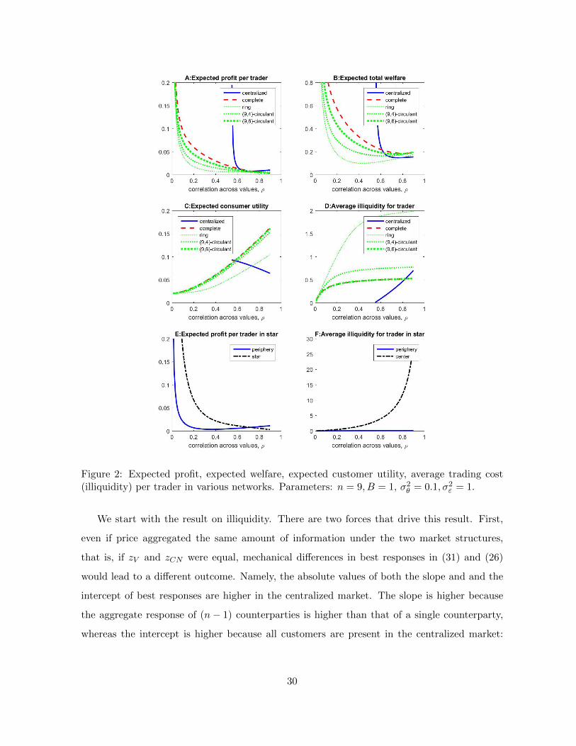
Figure 2: Expected profit, expected welfare, expected customer utility, average trading cost(illiquidity) per trader in various networks. Parameters: n = 9, B = 1, σ2
θ = 0.1, σ2ε = 1.
We start with the result on illiquidity. There are two forces that drive this result. First,
even if price aggregated the same amount of information under the two market structures,
that is, if zV and zCN were equal, mechanical differences in best responses in (31) and (26)
would lead to a different outcome. Namely, the absolute values of both the slope and and the
intercept of best responses are higher in the centralized market. The slope is higher because
the aggregate response of (n− 1) counterparties is higher than that of a single counterparty,
whereas the intercept is higher because all customers are present in the centralized market:
30
−βV = Bn > 2Bn−1 = −βCN . Whereas the slope and intercept have opposite effects, simple
algebra shows that the sum of these forces would result in higher illiquidity in the OTC market
as1tV1
tCN
|zv=zCN=z < 1.
Second, however, the single price in the centralized market aggregates more information
than each of the individual prices separately in the OTC market. Indeed, it is easy to check
that zCN < zV for any parameter values. This tends to make illiquidity higher in the OTC
market. Note that increasing the ratio zVzCN
increases illiquidity in the centralized market
relative to the OTC market as
∂1tV1
tCN
| zVzCN
=x
∂x=
∂− 2Bn−1
1z
−nBn(xz−1)+2−zx
∂x> 0.
Because zVzCN
is monotonically increasing in ρ, this force is strongest at the common value limit.
As we prove in the proposition, this effect is sufficient to make illiquidity higher for in OTC
market in the common value limit.
To understand the result on welfare, we start by comparing customers utility. Note first
that the ratio of customers’ utility in the complete network OTC market and the centralized
market is the ratio of the price variance in each market:Bn−1
n(n−1)2
E(p2CN)nB2E(p2V )
=E(p2CN)E(p2V )
. Also, in
the common value limit, the price variance is larger under the OTC structure as
limρ→1
E(p2CN
)E(p2V
) = limρ→1
(1
2+zCN
)24(V(ei)
+ V(ei, ej
))(
12+(n−1)zV
)22n (V (ei) + (n− 1)V (ei, ej))
=
(2n− 3
n− 1
)2
> 1.
As is apparent from the second expression above, there are two forces. On the one hand, in
a centralized market the variance of the price is connected to the variance of the sum of all
expectations, whereas in an OTC market, it is connected to the variance of the sum of the
two expectations at each link. The first one is higher, which makes customers’ expected utility
higher on centralized markets. On the other hand, as zV > zCN , the multiplier coming from
trading intensities tends to push customers’ utility higher in the OTC market. The ratio zVzCN
is maximal in the common value limit, and the second force turns out to dominate the first.
So in this limit, the utility is higher under the OTC structure. As Panels A-D in Figure 2
demonstrate, when ρ is smaller, the first force might dominate, thus implying that utility tends
31
to be larger under the centralized structure.
Finally, we explain why welfare is higher but the expected profit of dealers is lower in the
OTC market in the common value limit. For this, we substitute in the closed-form expressions
to (30), the sum of the value of allocations to dealers and customers. Taking the limit, it is easy
to show that the sum of terms corresponding to dealers is actually greater in the OTC market
than in the centralized market in the common value limit ρ → 1. This is due to the larger
trading intensity in OTC markets in this limit. The difference between formulas (29) and (30)
represents, essentially, a transfer from dealers to customers. Since this transfer is larger under
the OTC market structure, this explains why welfare and profit move in opposite directions. As
is apparent from the middle expression in (28), the total transfer is∑
ij
(−βijE
(p2ij
)), twice
the utility of customers, which, as we argued above, is indeed higher in the OTC complete
network than in the centralized market in the common value limit.
5.1.3 The effect of more links: circulant networks with varying density
Panels A-D in Figure 2 also illustrate how welfare, customers’ utility, dealers’ profit and illi-
quidity compares in various (n, k)-circulants. With fewer links, welfare and customers’ utility
tends to decrease and illiquidity tends to increase, whereas dealers’ profit might go either way.
As there are no explicit solutions for the conditional guessing game for circulant networks,
we do not have analytical results for the circulant OTC networks either. Nonetheless, because
of the symmetry, the intuition behind the numerical results is relatively simple. Decreasing the
number of links in symmetric fashion has two main effects: each dealer learns less and each
dealer has fewer opportunities to trade and intermediate. Learning less implies more concern
about adverse selection, lower trading intensities on average, higher illiquidity and smaller
variance of prices at each link (as fewer links implies lower variation in expectations as weights
on the common prior increase and weights on signals decrease). Fewer opportunities to trade
and smaller trading intensities imply a smaller trading volume which is the dominating force in
reduced welfare. The lower price variance implies a reduced customers’ utility and, by the logic
explained above, a smaller total transfer from dealers to customers. Profits can go either way
because the net effect of less trade and smaller transfers is ambiguous. As we see in the figure,
close to the common value limit, less dense networks might be more profitable for dealers.
32

5.1.4 The effect of asymmetry: periphery and the central dealer in a star network
The star network is an ideal case to study the effect of asymmetry on allocations and welfare.
The main result in this subsection is that central agents do not always earn higher expected
profit than periphery agents. In fact, expected profit is higher for periphery agents in the
common value limit.
Simple, closed-form solutions that characterize the equilibrium in a star network are spelled
out in Appendix B. The next proposition and Panels E-F in Figure 2 show analytical and
numerical results, respectively, concerning illiquidity, profit, and welfare.
Proposition 9 In a star network, the following statements hold
1. The adverse selection concern and the trading intensity of periphery traders are higher,
zP > zC , tP > tC , or, equivalently, the central dealer faces a more illiquid market than
the periphery dealers for any ρ.
2. In the common value limit, ρ → 1, central dealer’s profit converge to zero while the
periphery dealer”s profit is bounded away from zero as tP → −β, tC → 0.
We start by comparing the trading intensities, tP and tC . As we noted before, for the
central agent prices are privately fully revealing. That is, her posterior belief is the same as the
belief of dealers in a complete network or in a centralized market. In contrast, the learning of
periphery dealers is limited by the fact that they observe a single price only. As a result, the
weight that a periphery dealer puts on the price is larger than the weight the central dealer
puts on the same price, so zP > zC always holds. Intuitively, the periphery dealer is more
concerned about adverse selection than the central dealer, as the central dealer knows more.
Therefore, from (22), the trading intensity of periphery traders is always larger, as
tPtC
=2− zC2− zP
> 1.
Hence, at each link the central dealer trades with a smaller intensity, or equivalently, the market
is less liquid for the central dealer than for the periphery dealer.
The lesson from the above intuition is that a dealer trading with less-connected counter-
parties should face a higher price impact. In the special case of a star, the dealer with the
33
least-connected counterparties is the central dealer. Thus, in the star, there is a positive cor-
relation between price impact and number of own links. However, this is an artifact of the
special structure of the star. In more general core-periphery networks the average number
of links of more-connected dealers’ counterparties is often greater. Indeed, in our calibrated
example in Section 5.2, there is a negative relationship both between price impact and number
of counterparty’s links (just as in the star) and between price impact and number of own links
(unlike in a star).
Now, we turn to profits and allocations in the star network. Although the central dealer
trades with less intensity, she also trades and intermediates across more links, and by (23),
the distance between her expectation and the price is higher than for the periphery dealer. As
illustrated in Panels E-F in Figure 2, for a large set of parameter values, the effect of the smaller
trading intensity is dominated, and trading as a central agent is more profitable in expectation
than as a periphery agent. However, this is not always the case. As is apparent in the figure,
this statement is reversed as we approach the common value limit. In fact, in the limit the
expected profit of the central dealer is zero, whereas it is strictly positive for periphery dealers,
as we state in Proposition 9. Again, this is related to the strong negative assortativity in a
star.
To see the intuition, it is illustrative to specify how profits are determined close to the
common value limit. In the limit, all dealers put diminishing weight on their own signal as
they form expectations. Instead, in the conditional guessing game as ρ→ 1, periphery dealers
put a weight of zP → 1 on the expectation of the central dealer, while the central dealer puts
equal weight on each of the periphery agents’ expectations, implying zC → 1n−1 . Thus, by
Proposition 9, as we approach the common value limit in the OTC game, this implies trading
intensities of tP → −β, tC → 0. That is, central dealers do not trade in this limit at all, and
periphery dealers trade only with customers. In the common value limit, the central agent has
better information about the common value of the asset than periphery agents. Thus, as a
manifestation of the no-trade theorem, there cannot be an equilibrium where these agents trade
with each other. Therefore, the only remaining question is who trades with the customers. As
periphery agents are more concerned about adverse selection, the price impact of the central
dealer is larger. This implies that there is a price-quantity pair at which the central dealer
stops trading, but at which the periphery dealer is still willing to trade. This results in positive
34

trade between periphery and customers only.
5.2 Real-world OTC markets: a calibrated example
An attractive feature of our model is that it generates a rich set of empirical predictions. As
we emphasize in this section, for any given information structure and dealer network, our
model generates the full list of demand curves and the joint distribution of bilateral prices and
quantities, which we can use to calculate the expectations of price dispersion, intermediation,
trading volume and other financial variables. Therefore, in principle, our results could be
compared to stylized facts from the growing empirical literature using transaction-level OTC
data.
In this subsection, we give guidelines for future empirical work by an illustrative exam-
ple. Namely, we fit our parameters to the securitization market, i.e., the secondary market
of ABSs, CDOs, CMBs and non-agency CMOs, as presented by Hollifield et al. (2016). In
particular, conditioning on the reported dealer network, we explore the sensitivity of various
variables of interest to the parameters of our model, we find the parameters that match few
selected moments reported by Hollifield et al. (2016), and we analyze the model with the fitted
parameters.
5.2.1 The dealer network and sensitivity of moments
Hollifield et al. (2016) analyze the effect of the interdealer network on bid-ask spreads in
various segments of the securitization market using a transaction level data set from FINRA
during eight months in 2011-2012. Conveniently, in the working paper version, Hollifield et al.
(2013) report the filtered, 78-dealer representation of the trading network where only links with
sufficient frequency and size of transactions are reported. We reproduce this network on Figure
3. Using this network, we calculate the equilibrium of our model as described by Propositions
1and 2.
To give a sense of which empirical moments one can choose to fit our model to the data,
on Figure 4 we plot a number of objects for a range of parameters. In particular, we show the
mean price impact, the ratio of expected profit per dealer and expected net positions per dealer,
absolute and relative price dispersion, expected total gross volume, and mean expected profit
35
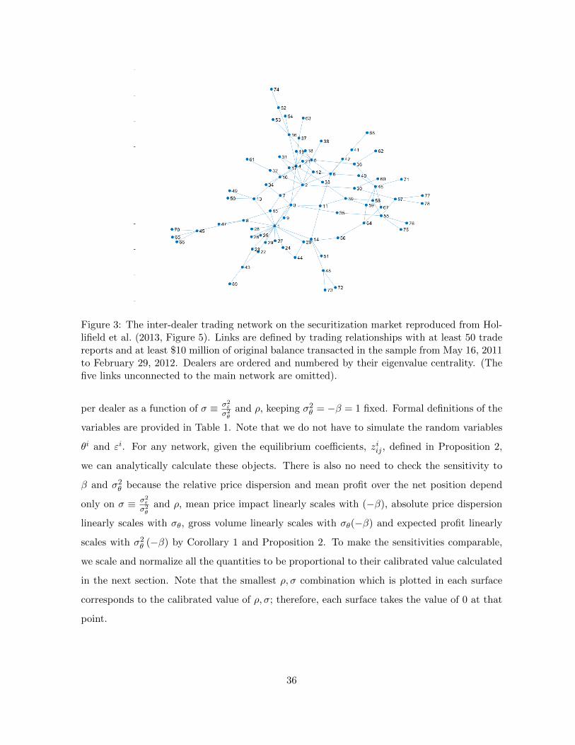
Figure 3: The inter-dealer trading network on the securitization market reproduced from Hol-lifield et al. (2013, Figure 5). Links are defined by trading relationships with at least 50 tradereports and at least $10 million of original balance transacted in the sample from May 16, 2011to February 29, 2012. Dealers are ordered and numbered by their eigenvalue centrality. (Thefive links unconnected to the main network are omitted).
per dealer as a function of σ ≡ σ2ε
σ2θ
and ρ, keeping σ2θ = −β = 1 fixed. Formal definitions of the
variables are provided in Table 1. Note that we do not have to simulate the random variables
θi and εi. For any network, given the equilibrium coefficients, ziij , defined in Proposition 2,
we can analytically calculate these objects. There is also no need to check the sensitivity to
β and σ2θ because the relative price dispersion and mean profit over the net position depend
only on σ ≡ σ2ε
σ2θ
and ρ, mean price impact linearly scales with (−β), absolute price dispersion
linearly scales with σθ, gross volume linearly scales with σθ(−β) and expected profit linearly
scales with σ2θ (−β) by Corollary 1 and Proposition 2. To make the sensitivities comparable,
we scale and normalize all the quantities to be proportional to their calibrated value calculated
in the next section. Note that the smallest ρ, σ combination which is plotted in each surface
corresponds to the calibrated value of ρ, σ; therefore, each surface takes the value of 0 at that
point.
36

moments formula
mean price impact 1mΣi
1|gi|Σj∈gi
1tiij
ratio of expected profit to expected net positions per dealerE(
1n
Σi∑ij∈gi q
iij(θi−pij)
)E(
1n
Σi|∑ij∈gi q
iij |)
absolute price dispersion
√E(
1mΣij (pij − p)2
)relative price dispersion
√E( 1
mΣij(pij−p)2)E(|p|)
expected total gross volume E(
ΣiΣj∈gi |qiij |)
mean expected profit per dealer E(
1nΣi
∑ij∈gi q
iij
(θi − pij
))Table 1: Moments and definitions.
5.2.2 Matching parameters
Ideally, we would estimate our parameters and test the fit by GMM in an over-identified system
of a large number of moments including the ones in Figure 4. However, because we do not have
access to the data set, we limit ourselves to the following exercise. We use three moments that
are reported in Hollifield et al. (2016) that have a natural counterpart in our model and respond
differently to our parameters: the average customer bid-ask spread, relative price dispersion,
and total volume.9 As we show in this subsection, these three moments exactly identify the
three free parameters of the model, σ ≡ σ2ε
σ2θ, (−β)σ2
θ and ρ. Then, using the fitted parameter
values we calculate various indicators to assess the strength and weaknesses of our framework.
We provide more details of this exercise in Appendix C.
Hollifield et al. (2016) constructs customer bid-ask spreads as follows. They identify trades
when a customer sells a given quantity to a dealer, which the dealer (potentially through other
dealers) passed on to another customer. The bid-ask spread is the difference between the two
transaction prices with the customers as a percentage of the value of the transaction. A single
dealer involved in 83% of these chains.
The variable that corresponds in our model to the customer bid-ask spread is price impact.
Indeed, from (13), the theoretical price difference for customers associated to a link ij of selling
and buying ∆ units from dealer j, pij (−∆)−pij (∆) , as a percentage of the marginal valuation
9For simplicity, we focus on one of the two main explored segments: the ”Rule 144a” securities. We choosethis segment because the average trade size is larger; therefore, we expect that the filtering of our base networkis less limiting.
37
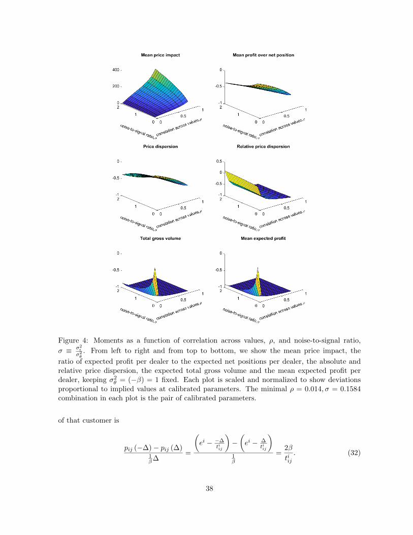
Figure 4: Moments as a function of correlation across values, ρ, and noise-to-signal ratio,
σ ≡ σ2ε
σ2θ. From left to right and from top to bottom, we show the mean price impact, the
ratio of expected profit per dealer to the expected net positions per dealer, the absolute andrelative price dispersion, the expected total gross volume and the mean expected profit perdealer, keeping σ2
θ = (−β) = 1 fixed. Each plot is scaled and normalized to show deviationsproportional to implied values at calibrated parameters. The minimal ρ = 0.014, σ = 0.1584combination in each plot is the pair of calibrated parameters.
of that customer is
pij (−∆)− pij (∆)1β∆
=
(ei − −∆
tiij
)−(ei − ∆
tiij
)1β
=2β
tiij. (32)
38
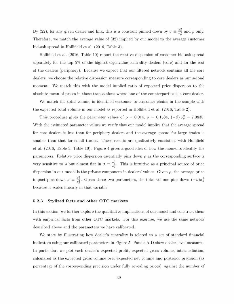
By (22), for any given dealer and link, this is a constant pinned down by σ ≡ σ2ε
σ2θ
and ρ only.
Therefore, we match the average value of (32) implied by our model to the average customer
bid-ask spread in Hollifield et al. (2016, Table 3).
Hollifield et al. (2016, Table 10) report the relative dispersion of customer bid-ask spread
separately for the top 5% of the highest eigenvalue centrality dealers (core) and for the rest
of the dealers (periphery). Because we expect that our filtered network contains all the core
dealers, we choose the relative dispersion measure corresponding to core dealers as our second
moment. We match this with the model implied ratio of expected price dispersion to the
absolute mean of prices in those transactions where one of the counterparties is a core dealer.
We match the total volume in identified customer to customer chains in the sample with
the expected total volume in our model as reported in Hollifield et al. (2016, Table 2).
This procedure gives the parameter values of ρ = 0.014, σ = 0.1584, (−β)σ2θ = 7.3835.
With the estimated parameter values we verify that our model implies that the average spread
for core dealers is less than for periphery dealers and the average spread for large trades is
smaller than that for small trades. These results are qualitativly consistent with Hollifield
et al. (2016, Table 3, Table 10). Figure 4 gives a good idea of how the moments identify the
parameters. Relative price dispersion essentially pins down ρ as the corresponding surface is
very sensitive to ρ but almost flat in σ ≡ σ2ε
σ2θ. This is intuitive as a principal source of price
dispersion in our model is the private component in dealers’ values. Given ρ, the average price
impact pins down σ ≡ σ2ε
σ2θ. Given these two parameters, the total volume pins down (−β)σ2
θ
because it scales linearly in that variable.
5.2.3 Stylized facts and other OTC markets
In this section, we further explore the qualitative implications of our model and constrast them
with empirical facts from other OTC markets. For this exercise, we use the same network
described above and the parameters we have calibrated.
We start by illustrating how dealer’s centrality is related to a set of standard financial
indicators using our calibrated parameters in Figure 5. Panels A-D show dealer level measures.
In particular, we plot each dealer’s expected profit, expected gross volume, intermediation,
calculated as the expected gross volume over expected net volume and posterior precision (as
percentage of the corresponding precision under fully revealing prices), against the number of
39

trading partners of the given dealer. Panels E-F show link level measures. In particular, we
plot the price impact a dealer faces on a given link against the number of trading partners,
and against the sum of the trading partners of the two counterparties connected by the link,
respectively.
The relationship between the degree of the dealer and her profit, gross volume, gross-to-
net volume ratio or precision is strong and positive. The shape of the scatter plots suggests
that, given the calibrated parameters, the dealer’s degree centrality summarizes almost all
the relevant information of her network position to determine her profit, volume, information
precision and gross-to-net volume ratio. While there is only a weak negative relationship
between the degree of the dealer and her price impact, there is a strong relationship between
the sum of the degrees of both counterparties and price impact. This is consistent with our
discussion in Section 5. The price impact a dealer faces is smaller when her counterparty
puts less weight on the given price, for example, because she trades with a large number of
counterparties. Therefore, we should observe the smallest price impact when both parties have
a large number of trading partners.10
These observations are qualitatively consistent with the empirical literature considering
various markets. Similarly to Hollifield et al. (2016), Di Maggio et al. (2017) find in the context
of the corporate bond market that central dealers offer lower spreads compared to periphery
dealers. Consistently with our analysis, they also find that the centrality of both counterparties
matter for price impact of the trade. They find that the price impact is lowest between two
high-centrality dealers, highest between two low-centrality dealers, and in-between when only
one of the counterparty has high centrality. This is as predicted by Panel F on Figure 5.11
Li and Schurhoff (2014) also show that central agents in the municipal bond market trade
more, their trades are more profitable, and they seem to be better informed than others. The
positive relationship between centrality and trading volume is also confirmed by Roukny et al.
(2014) for a data-set of European CDSs.
10As parameters vary the relationships shown in Figure 5 are always strong and have the same sign. However,especially as correlation, ρ, increases, degree centrality does not suppress all the other network characteristicsto the same extant. We illustrates this observation in Appendix C.
11Interestingly, in contrast to Hollifield et al. (2016) and Di Maggio et al. (2017), Li and Schurhoff (2014) findsthat central traders offer higher spreads than periphery traders in the context of the municipal bond market.Hollifield et al. (2016) suggests that the difference might be due to the different level of sophistication in thesemarkets. Our model suggests that in the municipal bond market adverse selection might not be the first orderdeterminant of variation in spreads.
40
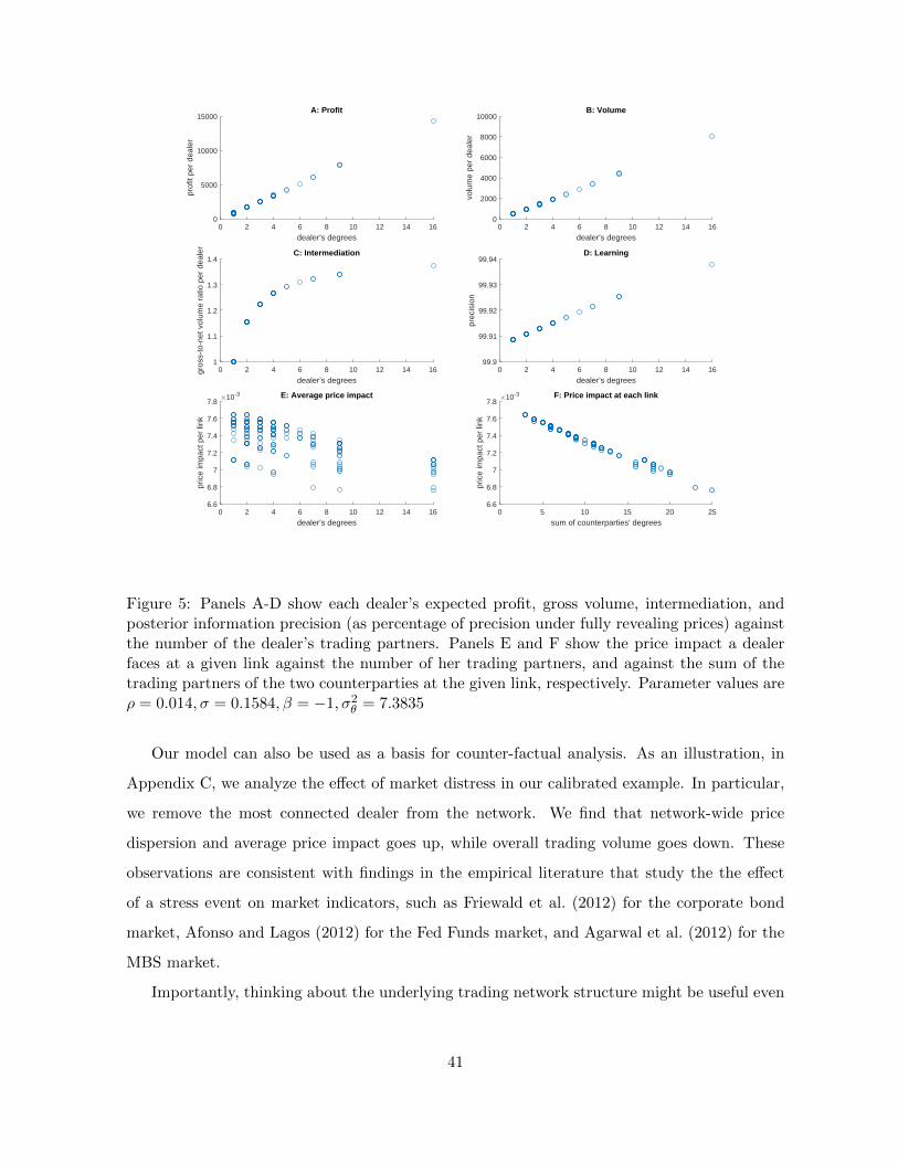
0 2 4 6 8 10 12 14 16
dealer's degrees
0
5000
10000
15000
prof
it pe
r de
aler
A: Profit
0 2 4 6 8 10 12 14 16
dealer's degrees
0
2000
4000
6000
8000
10000
volu
me
per
deal
er
B: Volume
0 2 4 6 8 10 12 14 16
dealer's degrees
1
1.1
1.2
1.3
1.4
gros
s-to
-net
vol
ume
ratio
per
dea
ler
C: Intermediation
0 2 4 6 8 10 12 14 16
dealer's degrees
99.9
99.91
99.92
99.93
99.94
prec
isio
n
D: Learning
0 2 4 6 8 10 12 14 16
dealer's degrees
6.6
6.8
7
7.2
7.4
7.6
7.8
pric
e im
pact
per
link
10-3 E: Average price impact
0 5 10 15 20 25
sum of counterparties' degrees
6.6
6.8
7
7.2
7.4
7.6
7.8
pric
e im
pact
per
link
10-3 F: Price impact at each link
Figure 5: Panels A-D show each dealer’s expected profit, gross volume, intermediation, andposterior information precision (as percentage of precision under fully revealing prices) againstthe number of the dealer’s trading partners. Panels E and F show the price impact a dealerfaces at a given link against the number of her trading partners, and against the sum of thetrading partners of the two counterparties at the given link, respectively. Parameter values areρ = 0.014, σ = 0.1584, β = −1, σ2
θ = 7.3835
Our model can also be used as a basis for counter-factual analysis. As an illustration, in
Appendix C, we analyze the effect of market distress in our calibrated example. In particular,
we remove the most connected dealer from the network. We find that network-wide price
dispersion and average price impact goes up, while overall trading volume goes down. These
observations are consistent with findings in the empirical literature that study the the effect
of a stress event on market indicators, such as Friewald et al. (2012) for the corporate bond
market, Afonso and Lagos (2012) for the Fed Funds market, and Agarwal et al. (2012) for the
MBS market.
Importantly, thinking about the underlying trading network structure might be useful even
41

when the econometrician has only limited information about dealers’ characteristics. Indeed,
given our results, we should expect that larger transaction size is associated with lower trading
costs, higher profits, profitable and more informative trades. The reason is that these are
properties of transactions of more connected dealers. From this set of predictions, the pattern
that percentage cost is decreasing in the size of the transaction is a robust observation in many
different contexts (see Green et al. (2007) and Li and Schurhoff (2014) on municipal bonds and
Edwards et al. (2007) and Randall (2015) on US corporate bonds).
Finally, consistent with our observations Atkeson et al. (2012), Li and Schurhoff (2014)
and Hollifield et al. (2016) all report the CDS and the securitized loan markets are highly
concentrated. While the same is true when US corporate bonds are evaluated in the aggregate,
Schultz (2001) reports that trading in specific bonds seems to be spread across multiple dealers.
Our model is silent on these differences.
6 The Price-Discovery Game
In this section, we guide the reader to better connect our OTC game to the real world features
of trading in OTC markets. In the OTC game dealers’ trading strategies are represented by
generalized demand curves, and all trades take place simultaneously. This is a very tractable
and rich theoretical structure, and we consider the one-shot OTC game as a reduced-form
representation of how equilibrium prices and quantities are determined in reality.
In real world OTC markets, dealers do not post full demand curves. Instead, dealers engage
in bilateral negotiations with their counterparties by quoting prices which are valid for a certain
quantity. To capture this feature, we introduce a variant of the OTC game where dealers find
the equilibrium prices and quantities through a sequence of bilateral exchange of quotes.
In particular, consider that each node in a given network is a trading desk. Each desk i
consists of a desk-head, whom we continue to refer as dealer i, and one or more traders. Dealer
i designs a bidding strategy and the traders have to implement this strategy. The bidding
strategy describes how the traders should respond to bids they receive from counterparties.
Bidding takes place sequentially, in rounds. In each bidding round τ , each trading desk i
makes an offer πiij,τ ={piij,τ , q
iij,τ
}to each trading desk j with whom she has a link, indicating
that she is willing to trade quantity qiij,τ for price piij,τ . Thus, in any bidding round all dealers
42

make and receive offers to and from their counterparties in the network. If the price offered
by i to j is arbitrarily close to the price offered by j to i, and the two quantities differ only to
the extent of the order of the customers’ demand at the given price, then the offer is accepted.
Otherwise, a trading desk j that receives the bid in round τ , responds with a counter-offer
πjij,τ+1 ={pjij,τ+1, q
jij,τ+1
}in round τ +1. This process can continue for any number of rounds,
until all trading desks accept the offers. At that point, trades are executed both across dealers
and with customers. We define this game formally in the appendix and call it a price-discovery
game.
The following proposition proves our claim that dealers can find the equilibrium prices and
quantities in the OTC game by playing the price-discovery game.
Proposition 10 Suppose that there exists an equilibrium in the OTC game, with yi ≥ 0 and
ziij ≥ 0 whenever j ∈ gi.
1. There exists a set of bidding strategies that are an equilibrium in the price-discovery game.
2. The resulting prices and quantities are the same as the equilibrium prices and quantities
in the OTC game.
Although the construction of the price-discovery game is arguably artificial, it illustrates
some important features of our OTC game. On the one hand, finding the equilibrium prices
and quantities in the OTC game needs not rely on any kind of auctioneer. The price-discovery
game shows that equilibrium prices and quantities can be found via an iterative, decentralized
process. Moreover, the coefficients of the generalized demand curves (and, consequently the
coefficients of the bidding strategies) can be derived without observing the realization of signals.
Indeed, dealers can find the equilibrium coefficients just by understanding the structure of the
game they are facing.
On the other hand, the price discovery game emphasizes an important limitation of the
OTC game. Namely, the equivalence between the price discovery game and the OTC game
relies on the fact that the bidding strategies are static. That is, they do not depend on the
bidding round, and they are conditional only on the outcome of the last bidding round, as
opposed to all previous rounds. This restriction on the strategy space of dealers that dealers
can use is necessary as the OTC game is nevertheless a static game. Thus, in our framework,
43

we are unable to capture any dynamic learning considerations inherent in real-world OTC
markets.
7 Conclusions
In this paper, we proposed a model of trading and information diffusion in OTC markets.
Dealers trade on a fixed network, and each dealer’s strategy is represented as a quantity-
price schedule. We showed that information diffusion through prices is unaffected by dealers’
strategic trading motives and that each price partially incorporate the private information of
all dealers, and we identified an informational externality that constrains the informativeness
of prices. We also highlighted that trade decentralization can both increase or decrease welfare
and that the main determinant of a dealer’s trading cost is not her centrality but rather the
centrality of her counterparties. We used a calibrated example and various robustness checks to
illustrate that in realistic interdealer networks, more-central dealers learn more, intermediate
more, trade more at lower costs and earn higher expected profit.
Importantly, trading protocols in OTC markets have become increasingly diverse. There
are a number of protocols (e.g., dealer runs, broker-assisted work-up protocols), which our
paper does not address explicitly. Given this increasing diversity, it is important to develop
frameworks that put limited emphasis on any one particular trading protocol and can still cap-
ture robust features of OTC markets. Our approach emphasizes that links are persistent, that
the market structure is concentrated, and that dealers intermediate trade between otherwise-
disconnected counterparties. Our model yields price-quantity pairs that are consistent with
each dealers information, potential trading partners and objectives. We implicitly suggest that
if such pairs exists, it is likely that the market will converge to these points, independently of
the trading protocol.
Demand and supply curves have been a powerful tool to model equilibrium in centralized
good markets since the beginning of economic thinking. Using our approach of generalized
demand curves on networks, we have also found a method to obtain insights for decentralized
markets.
44
References
Acemoglu, D., M. A. Dahleh, I. Lobel, and A. Ozdaglar (2011): “Bayesian Learningin Social Networks,” The Review of Economic Studies, 78, 1201–1236.
Afonso, G. and R. Lagos (2012): “Trade Dynamics in the Market for Federal Funds,” Tech.rep., Federal Reserve Bank of New York Staff Reports, 549.
Agarwal, S., Y. Chang, and A. Yavas (2012): “Adverse selection in mortgage securitiza-tion,” Journal of Financial Economics, 105, 640–660.
Atkeson, A. G., A. L. Eisfeldt, and P.-O. Weill (2012): “The Market for OTC CreditDerivatives,” Sites.google.com/site/pierreolivierweill.
Bala, V. and S. Goyal (1998): “Learning from Neighbours,” The Review of EconomicStudies, 65, 595–621.
Choi, S., A. Galeotti, and S. Goyal (2013): “Trading in Networks: Theory and Experi-ment,” Http://www.homepages.ucl.ac.uk/ uctpsc0/.
Colla, P. and A. Mele (2010): “Information Linkages and Correlated Trading,” Review ofFinancial Studies, 23, 203–246.
Condorelli, D. and A. Galeotti (2012): “Bilateral Trading in Networks,”Http://privatewww.essex.ac.uk/ dcond/TRADNET.pdf.
DeMarzo, P., D. Vayanos, and J. Zwiebel (2003): “Persuasion Bias, Social Influence,and Unidimensional Opinions,” The Quarterly Journal of Economics, 118, 909–968.
Di Maggio, M., A. Kermani, and Z. Song (2017): “The value of trading relations inturbulent times,” Journal of Financial Economics, 124, 266–284.
Duffie, D. (2012): Dark markets: Asset pricing and information transmission in over-the-counter markets, Princeton University Press.
Duffie, D., N. Garleanu, and L. H. Pedersen (2005): “Over-the-Counter Markets,”Econometrica, 73, 1815–1847.
Duffie, D., N. Grleanu, and L. H. Pedersen (2007): “Valuation in Over-the-CounterMarkets,” Review of Financial Studies, 20, 1865–1900.
Duffie, D., S. Malamud, and G. Manso (2009): “Information Percolation With Equili-brium Search Dynamics,” Econometrica, 77, 1513–1574.
Edwards, A. K., L. E. Harris, and M. S. Piwowar (2007): “Corporate Bond MarketTransaction Costs and Transparency,” Journal of Finance, 62, 1421–1451.
Friewald, N., R. Jankowitsch, and M. G. Subrahmanyam (2012): “Illiquidity or creditdeterioration: A study of liquidity in the US corporate bond market during financial crises,”Journal of Financial Economics, 105, 18–36.
Gale, D. and S. Kariv (2007): “Financial Networks,” American Economic Review, Papers& Proceedings, 92, 99–103.
Gofman, M. (2011): “A Network-Based Analysis of Over-the-Counter Markets,”Https://mywebspace.wisc.edu/gofman/web/JMP/MichaelGofmanJMP.pdf.
Golosov, M., G. Lorenzoni, and A. Tsyvinski (2009): “Decentralized Trading withPrivate Information,” NBER Working Papers 15513, National Bureau of Economic Research,Inc.
Golub, B. and M. O. Jackson (2010): “Naive Learning in Social Networks: Convergence,Influence, and the Wisdom of Crowds,” American Economic Journal: Microeconomics, 2,112–149.
Green, R. C., B. Hollifield, and N. Schurhoff (2007): “Dealer intermediation and
45
price behavior in the aftermarket for new bond issues,” Journal of Financial Economics, 86,643–682.
Hendershott, T., D. Li, D. Livdan, and N. Schurhoff (2016): “Relationship tradingin OTC markets,” Tech. rep., Swiss Finance Institute.
Hollifield, B., A. Neklyudov, and C. Spatt (2013): “Bid-ask spreads and the pricing ofsecuritizations: 144a vs registered securitizations,” ASSA meeting 2014.
——— (2016): “Bid-Ask Spreads, Trading Networks, and the Pricing of Securitizations,” TheReview of Financial Studies, forthcoming.
Kranton, R. E. and D. F. Minehart (2001): “A Theory of Buyer-Seller Networks,” Ame-rican Economic Review, 91, 485–508.
Kyle, A. S. (1989): “Informed Speculation with Imperfect Competition,” Review of EconomicStudies, 56, 317–55.
Lagos, R. and G. Rocheteau (2009): “Liquidity in Asset Markets With Search Frictions,”Econometrica, 77, 403–426.
Lagos, R., G. Rocheteau, and P.-O. Weill (2008): “Crashes and Recoveries in IlliquidMarkets,” NBER Working Papers 14119, National Bureau of Economic Research, Inc.
Li, D. and N. Schurhoff (2014): “Dealer networks,” Tech. rep., CEPR Discussion PaperNo. DP10237.
Malamud, S. and M. Rostek (2013): “Decentralized Exchange,” Tech. rep., EPFL,http://papers.ssrn.com/sol3/papers.cfm?abstract id=2164332.
Manea, M. (2013): “Intermediation in Networks,” Http://economics.mit.edu/faculty/manea/papers.Meyer, C. D. (2000): Matrix analysis and applied linear algebra, Philadelphia, PA, USA:
Society for Industrial and Applied Mathematics.Nava, F. (2013): “Efficiency in Decentralized Oligopolistic Markets,”
Http://personal.lse.ac.uk/nava/research.htm.Ozsoylev, H. and J. Walden (2011): “Asset Pricing in Large Information Networks,”
Journal of Economic Theory, 146, 2252–2280.Rahi, R. and J.-P. Zigrand (2006): “Arbitrage networks,” Open Access publications from
London School of Economics and Political Science http://eprints.lse.ac.uk/, London Schoolof Economics and Political Science.
Randall, O. (2015): “Pricing and liquidity in the US corporate bond market,” Emory Uni-versity.
Roukny, T., C.-P. Georg, and S. Battiston (2014): “A network analysis of the evolu-tion of the German interbank market,” Discussion Papers 22/2014, Deutsche Bundesbank,Research Centre.
Schultz, P. (2001): “Corporate bond trading costs: A peek behind the curtain,” The Journalof Finance, 56, 677–698.
Vayanos, D. and P.-O. Weill (2008): “A Search-Based Theory of the On-the-Run Pheno-menon,” Journal of Finance, 63, 1361–1398.
Vives, X. (2011): “Strategic Supply Function Competition With Private Information,” Eco-nometrica, 79, 1919–1966.
Walden, J. (2013): “Trading, Profits, and Volatility in a Dynamic Information NetworkModel.” Working paper University of Berkeley.
46
A Appendix: Proofs
In some proofs we use the convention that a network, g, can be represented by an adjacencymatrix A (g) with elements Aij = 1 if ij ∈ g, and Aij = 0 if ij /∈ g. Also, sometimes weuse matrix notation as follows. V, Z, Y are n× n matrices of row vectors vi, yi, zi,, i = 1, ..., nrespectively. The individual elements of V are vij . The individual element of Z is ziij iff Aij = 1
and 0 otherwise, while Y is a diagonal matrix with yi at its i-th diagonal element.
Proof of Proposition1
We prove the statement in a more general form than stated. It proves existence for a generalGaussian information structure. We need only that if ωi is a column vector of the covariancesbetween θi and each of the signals (in our case it is ωii = σ2
θ and ωij = ρσ2θ for i 6= j), then
ωi > 0 for all i. Note that we can rewrite the problem as follows. We are looking for a V ∗
matrix of which each row vi is the solution of the problem of
maxyi,zi
(2viωi − viΣ(vi)>
)(A.1)
s.t. vi =[yi + ziV ∗
]ziij = 0⇐⇒ Aij = 0
where Σ is the covariance matrix of signals, s, and yi is a row vector with a yi at the i−th placeand 0 otherwise, while zi is a row vector of size n with elements of some (ziij)j=1,..n (subject tothe last constraint).
To see that this V ∗ exists, let us first define the matrix mapping F : Rn×n → Rn×n, whichmaps any n× n matrix V 0 to another one with rows (vi)i=1,...,n defined by
vi ≡ arg maxyi,zi
(2viωi − viΣ(vi)>
)(A.2)
s.t. vi =[yi + ziV 0
]ziij = 0⇐⇒ Aij = 0
Further, let
Vi ≡ {vi : viΣ(vi)> − 2viωi +ω2ii
Σii≤ 0}.
and Vn×n ≡ V1 × V2..× Vn be the set of matrices with rows vi ∈ Vi.We need to show that F is a continuous self map with respect to the set of matrices Vn×n
and that Vn×n is a convex compact set. Hence, the Brouwer fixed-point theorem applies. Weproceed in steps.
1. We show that F defined by (A.2) is a self-map.
For this, note that increasing the number of 0-s in the i − th row of A (decreasing thenumber of links to i in the network) adds more constraints to the problem (A.2). So weconsider the extreme problem where the i− th row and column of A has only zeros, that
47

is, each ziij ≡ 0. It is easy to show that in this case the problem reduces to
ω2ii
Σii= max
vii[2viiωii − viiΣiivii]
with a solution of yi = vii = ωiiΣii
and vij = 0 for all i 6= j. Thus, for any A with non-zero
elements in the i − th row and column,ω2ii
Σiiis a lower bound on the value agent i can
achieve, that is, the solution vi will satisfyω2ii
Σii≤ 2viωi − viΣ(vi)>. Implying that for
any V0 and A, F projects to Vnxn.
2. F is continuous in V 0 by the Maximum Theorem.
3. Given that the Cartesian product of convex and compact sets is also convex and compact,we only have to show that each Vi is convex, closed and bounded
(a) Vi is convex. Under the assumption that Σ is positive definite, viΣ(vi)>−2viωi is aconvex function (the sum of a convex and a linear function). From the fact that thesub-level sets of a convex functions are convex, it follows that the set Vi is convex.
(b) Vi is closed. Let g(vi) ≡ viΣ(vi)>−2viωi+ω2ii
Σiibe a function from Rn to R. Clearly,
g is continuous and Vi ≡ {vi : g(vi) ≤ 0}. Let vin, n = 1...∞ be a convergent seriesof vectors in Vi with vi∞ being the limit point of this series. Since g is continuous,we have g(vi∞) = limn→∞ g(vi∞) ≤ 0. Hence vi∞ ∈ Vi.
(c) Vi is bounded. Note that the function g(vi) is strictly convex, continuous, andtwice-differentiable. Hence, there exists a minimum vimin that g(vimin) ≤ g(vi) forall vi ∈ Vi Also, from the definition Vi, g(vi) ≤ 0 for all vi ∈ Vi. Note also that g(·)is strongly convex on Vi as there exists m > 0 such that ∇2g(v) −mI =2Σ −mIis positive definite (for example, one can pick m = σ2
θ + σ2ε). Also, from strong
convexity
g(v′′) ≥ g(v
′) +∇g(v
′)(v
′′ − v′)> +
m
2||v′′ − v
′ ||22.
for any v′,v′′ ∈ Rn. In particular, for v
′= vimin, we have ∇g(vimin) = 0 implying
thatg(v
′′)− g(vimin) ≥ m
2||v′′ − vimin||22.
Let us pick v′′
= vi an arbitrary element of Vi. Then g(v′′) ≤ 0 implying
− 2
mg(vimin) ≥ ||vi − vimin||22
proving the claim.
Proof of Proposition 2 and Corollary 1
Consider an equilibrium of the conditional guessing game in which
E(θi∣∣si, egi ) = yisi +
∑k∈gi
ziikE(θk∣∣∣sk, egk )
48

for every i. If the system (21) has a solution, then
E(θi∣∣si, egi ) =
yi(1−
∑l∈gi
ziil2−zlli
4−ziilzlli
)si +∑k∈gi
ziik
2−ziik4−ziikz
kki(
1−∑l∈gi
ziil2−zlli
4−ziilzlli
)E(θk∣∣∣sk, egk ) (A.3)
holds for every realization of the signals, and for each i. Now we show that choosing the pricesand demand functions (23) and (24) is an equilibrium of the OTC game.
First note that (26) for i and j at a given link implies (22). Also, the choice (24) implies
E(θi∣∣si, egi ) = yisi +
∑k∈gi
ziikpij = E(θi∣∣si,pgi ). (A.4)
The second equality comes from the fact that the first equality holds for any realization ofsignals and the projection theorem determines a unique linear combination with this propertyfor a given set of jointly normally distributed variables. Thus, (24) for each ij link is equivalentwith the corresponding first order condition (10). Finally, (A.4) also implies that the bilateralclearing condition between a dealer i and dealer j that have a link in network g
tiij(E(θi
∣∣si,pgi )− pij)+ tjij(E(θj
∣∣sj ,pgj )− pij)
+ βijpij = 0
is equivalent to (23). That concludes the statement.
Corollary 1 follows from the direct observation of (23) and (24) and (22).
Proof of Proposition 3
Case 1: Circulant networksWe provide here a draft of the proof. Further details of each step is available on request.Step 1 : We show that for circulant networks, each ziij > 0 for any ρ ∈ (0, 1) .
1. First, we show that ziij > 0 in the limit ρ→ 0. Clearly when ρ = 0, the equilibrium V is adiagonal matrix as the signals of others are uninformative in this pure private value case.The starting point is to show that for diminishingly small ρ, the off-diagonal elements ofV which are corresponding to first neighbors are diminishing at a slower rate than therest of the off-diagonal elements. In particular, we conjecture and verify that there areconstants a0 and a1 that
limρ→0
(V − a0I
ρ
)= a1A
where I and A are the identity matrix and the adjacency matrix respectively. For this,we calculate the matrices Y and Z which correspond to a starting matrix V 0 = a0I+a1Afor a given a0 and a1 in problem (A.2), obtain the resulting new matrix V 1 =
(Y + ZV 0
),
observe that each non-zero element in Z, ziij > 0 are positive, and verify there are indeed
a0 and a1 values for which limρ→0
(V 1−a0I
ρ
)= a1A.
2. Given that all ziij are positive in this limit, let us counterfactualy assume that there is
49
ρ ∈ (0, 1) for which at least one ziij < 0. By continuity, then must be a ρ0 for which all
ziij ≥ 0 but at least one of them is zero. But this implies that for these parameters dealer ifinds the expectation of one of her neighbors uninformative. Let {ik}k=1,...,mi be the set of
i’s neighbors and, without loss of generality, suppose that the index of this neighbor is mi.The only way this holds is that there is a linear combination of si and
{eik}k=1,...,(mi−1)
which replicates eimi , that is, that there is an arbitrary vector [λ0, λ1..λmi−1], that
λ0si + λ1e
i1 + ...λmi−1ei(mi−1) = eimi (A.5)
(a) Note that if the network is circulant, there must be an equilibrium where V is alsocirculant. To see this, note that problem (A.2) maps circulant networks into circulantnetworks. Also, given that we prove the properties of Vn×n vector-by-vector in theproof of 1, repeating those steps proves the existence of a circulant V fixed point.Furthermore, in this equilibrium the rows corresponding to the expectation of agenti and j has to have the structure of vi(i+l) = vi(i−l) = vj(j+l) = vj(j−l) for every l ≥ 0as long as n ≥ i − l, i + l, j − l, j + l ≥ 1. This is, the weight of each signal in theequilibrium expectation of a given dealer can depend only on whether that signalbelongs to a first neighbor, or a second neighbor etc. of the given dealer. This iscoming from the symmetry across dealers in circulant networks and the symmetricinformational content of their expectations in this equilibrium.
(b) However, given this symmetric structure of the equilibrium V matrix, there are novij and [λ0, λ1..λmi−1] values which can solve the equations (A.5) unless all vij arethe same. For instance, let us spell this out the implied equation system for the firstagent in a (7, 4) circulant network with k being the second neighbor. If the row ofV corresponding to the expectation of the first neighbor of 1 has the structure ofv1 v0 v1 v2 v3 v3 v2 then his second neighbor must have the structure ofv2 v1 v0 v1 v2 v3 v3 . Thus, we need
λ0
1000000
+ (λ1 + λ2)
v1
v0
v1
v2
v3
v3
v2
= (1− λ3)
v2
v1
v0
v1
v2
v3
v3
to hold for some scalars. It is easy to check that this implies that all v − s areidentical. However, it is also easy to check that a V with identical elements cannotbe a fixed point.
This is a contradiction which concludes step 1.Step 2 : We show that ziij < 1for any ρ ∈ (0, 1) .
For this, note that by using forward induction on the fixed point equation V = Y + ZV, we
50
obtain that the equilibrium matrix V must satisfy
V = Y limu→∞
u∑0
(Z)u
+ limu→∞
(Z)u+1
V.
As ρ ∈ (0, 1) the diagonal of Y must be strictly positive, as si must contain residual informationon the private value element of θi relative to the guesses of others. We know from Proposition1 that V exists. From the fact that all elements of Z are non-negative and from the fact thatthe Neumann series limu→∞
∑u0
(Z)u
converges if and only if limu→∞(Z)u+1
= 0 (see Meyer
(2000) page 618), we must have that indeed limu→∞(Z)u+1
= 0. As Z must be symmetricfor a circulant network, and all elements are non-negative, if any elements were larger than 1,then there were some elements of limu→∞
(Z)u+1
which would not diminish (as the elements(ziij
)u+1will be a component in some elements of the the matrix
(Z)u+1
for any i and j).
Step 3 : Now, we search for equilibria such that beliefs are symmetric, that is
ziij = zjji
for any pair ij that has a link in network g.The system (21) becomes
yi(1−
∑k∈gi
ziik2−ziik
4−(ziik)2
) = yi
ziij
2−zij4−z2ij(
1−∑k∈gi
ziik2−ziik
4−(ziik)2
) = ziij
for any i ∈ {1, 2, ..., n}. Working out the equation for ziij , we obtain
ziij2 + ziij
= ziij
1−∑k∈gi
ziik2 + ziik
and summing up for all j ∈ gi
∑j∈gi
ziij2 + ziij
=∑j∈gi
ziij
1−∑k∈gi
ziik2 + ziik
.
Denote
Si ≡∑k∈gi
ziik2 + ziik
.
51

Substituting above and summing again for j ∈ gi
Si
1 +∑j∈gi
ziij
=∑j∈gi
ziij
or
Si =
∑j∈gi
ziij(1 +
∑j∈gi
ziij
) .We can now obtain
ziij =2ziij
(1− Si
)1− ziij (1− Si)
(A.6)
andyi = yi
(1− Si
).
Finally, the following logic show that ziij ≤ 2. As ziij < 1, 2ziij <
(1 +
∑j∈gi
ziij
)implying that
2ziij(1− Si
)< 1 or 2ziij
(1− Si
)< 2
(1− ziij
(1− Si
)), which gives the result by A.6.
Case 2: Star networksWe give the closed-form solutions for the star network in Appendix B.2. One can check by
straightforward algebra that the resulting ziij are indeed in the [0, 2] interval.
Proof of Proposition 4
In an equilibrium of the OTC game, prices and quantities satisfy the first order conditions (10)and must be such that all bilateral trades clear.
Since market clearing conditions (6) are linear in prices and signals, we know that eachprice (if an equilibrium price vector exists) must be a certain linear combination of signals.Thus, each price is normally distributed.
From the first order conditions we have that
qiij(si,pgi) = tiij
(E(θi
∣∣si,pgi )− pij) .The bilateral clearing condition between a trader i and trader j that have a link in network gimplies that
tiij(E(θi
∣∣si,pgi )− pij)+ tiij(E(θj
∣∣sj ,pgj )− pij)
+ βijpij = 0
and solving for the price pij we have that
pij =tiijE(θi
∣∣si,pgi ) + tiijE(θj∣∣sj ,pgj )
tiij − βij
Since agent i knows E(θi∣∣si,pgi ), by definition, the vector of prices pgi is informationally
52
equivalent for her with the vector of posteriors of her neighbors Egi ={E(θj
∣∣sj ,pgj )}j∈gi .
This implies thatE(θi
∣∣si,pgi ) = E(θi∣∣si,Egi ).
Note also that as each price is a linear combination of signals and E(θj |·)
is a linear operator onjointly normal variables, there must be a vector wi that E(θi
∣∣si,pgi ) = E(θi∣∣si,Egi ) = wis.
That is, the collection of{wi}i=1,...n
has to satisfy the system of n equations given by
wis =E(θi∣∣∣si,{wjs
}j∈gi )
for every i. However, the collection{wi}i=1,...n
that is a solution of this system, is also anequilibrium of the conditional guessing game by construction.
Proof of Proposition 5
Equation (23), the fact that tiij > 0 for all i and j, and E(θi∣∣si,pgi ) = E(θi
∣∣si,Egi ) = visfrom Proposition 4 implies that we only have to show that all elements of the equilibrium Vmatrix defined in the proof of Proposition 1 are strictly positive.
We use the notation of Proposition 1. Vi is a convex set and must contain some strictly
positive vectors as the one minimizing g(·), defined above,(vi)min ≡ Σ−1ωi, is strictly positive
by assumption. Now we show that there it contains only a single point, the one for vii = ωiiΣii
and vij = 0 for all i 6= j, which is in any of the axes of Rn. This is sufficient to prove that vectorsin Vi cannot have negative elements as for a convex set to cross any of the axes, it should haveat least two points on that given axis. We show this by contradiction. Assume that vi ∈ Vihas an other elements on any of the axes, e.g. a vi such that vi1 = vi2 = ... = vin−1 = 0 andvin = x. Then g(·) simplifies to
g(vi) = x2Σnn − 2xωin +ω2ii
Σii,
The function attains a minimum at x∗ = ωinΣnn
. The minimum value of the function is − ωinΣnn
.
Therefore vi is not an element of Vi if
ω2in
Σnn<ω2ii
Σii.
But this always holds in our parameterization (asω2in
Σnn=
(ρσ2θ)
2
σ2θ+σ2
εand
ω2ii
Σii=
(σ2θ)
2
σ2θ+σ2
ε).
As we showed in Proposition 1, for any network and any parameters V must be in theCartesian product of Vn×n. However, the previous argument shows that there is a singlematrix which has not strictly positive elements, the diagonal matrix with vii = ωii
Σiifor all i.
But it is simple to check that this cannot be a fixed point of our system for any connectednetwork and any parameters as long as ρ 6= 0.
53
Proof of Proposition 6
1. From Proposition 4 we know that in any equilibrium of the OTC game
E(θi|si,pgi) = E(θi|si, egi).
Also, Lemma 5 shows that each equilibrium expectation in the conditional guessing gameis a linear combination of all signals in the economy
E(θi|si, egi) = vis
where vi > 0 for all i. That is, when the dealer network is complete, through prices, eachdealer observes (n− 1) linear combinations of s apart from her own private signal. Clearly,as long as these linear combinations are independent, the statement holds. Instead, letus assume that there exists a β, that E(θi|si, egi) = vis = βvjs =E(θj |sj , egj ) for some iand j. These two agents are connected (as everyone else). However, for any ρ < 1, this isimpossible, because at least one of the agents would find that putting a different weighton its own signal si improves over its estimate of θi over the best estimate of agent j onθj . Implying that either vis vjs is not an equilibrium of the conditional guessing game,implying that it cannot be an equilibrium guess in the OTC game either (by Proposition2).
2. Given joint normality, we only have to show that limρ→1E(θi|si,pgi
)= E
(θi|s)
andlimρ→1 var
(θi|si,pgi
)= var
(θi|s). We proceed in steps.
(a) Note that when ρ = 1, there exists an equilibrium of the conditional guessing game,(egi)i=1,...n
where E(θi|si, egi
)= E
(θi|s)
and var(θi|si, egi
)= var
(θi|s)
for all
i.This is so, because when ρ = 1, the best guess, E(θi|s), for each agent conditi-
onally of observing each signal is the same across agents. Therefore, if any agentwere to pick this guess, all of its neighbors would and could pick the same guess (byputting a weight of 1 on this guess). That is, it is a fixed point as defined by theequilibrium in the conditional guessing game.
(b) We argue this equilibrium is unique. For this, note that with ρ = 1, the equi-librium guess of agent i, vis has to be identical of that of agent vjs, for anypair of agents. The reason is that otherwise, there exists two linked agents, i, k
with vjs 6= vks, which implies either (1) differing values,e.g.,(2viωi − viΣ(vi
)>>(
2vkωk − vkΣ(vk)>)
, where we use the notation in the proof of Proposition 1.
However, in this case, because ρ = 1, agent k would be motivated to put a weight of1 to the guess of agent i, to obtain the same value as agent i does. Which is a contra-
diction of the claim that vks is an equilibrium guess. Or (2) if(
2viωi − viΣ(vi)>)
=(2vkωk − vkΣ
(vk)>)
but vjs 6= vks, then a convex combination of vjs and vks is
a feasible guess for any of the agents which improves their value. This is also acontradiction of the claim that vjs,vks were equilibrium guesses. However, if allagents have the same guesses, then this guess has to be the best guess E
(θi|s).
Otherwise, any agent would put a non-zero weigh on his own signal to improve onthis guess, leading to different equilibrium guesses across agents; a contradiction.
54
(c) By the continuity of the conditional guessing game in ρ, whenever ρ is sufficientlyclose to one any equilibrium must be arbitrarily close to the one at ρ = 1, implying
limρ→1
E(θi|si, egi
)= E
(θi|s)
limρ→1V(θi|si, egi
)= V
(θi|s).
(d) Following the argument in Proposition 2, if the equilibrium of the OTC game existsfor a ρ sufficiently close to 1, it is based on an equilibrium of the conditional guessinggame. Therefore for any agent the equilibrium price vector pgi is informationallyequivalent to the guess vector egi in the conditional guessing game, implying theresult.
Proof of Proposition 7
Observe that by symmetry across periphery dealers, V =(I − Z
)−1Y, for star network has
the elements of
v11 = yC1
1− (n− 1) zC zP
vi1 = yCzP
1− (n− 1) zC zP
vii = yP1− (n− 2) zC zP1− (n− 1) zC zP
v1i = yPzC
1− (n− 1) zC zP
vij = yPzC zP
1− (n− 1) zC zP
where yC , yP are the weights on the private signal and zC , zP are the weights on the others’guesses in the central and periphery agents’ guessing function respectively. As maximizing
E(−(θ − ei
)2)is equivalent with maximizing
2tr (V Σθs)− tr(V ΣV >
)where Σii = 1 + σ2,Σij = ρ, [Σθs]ii = 1, [Σθs]ij = ρ, we calculate the expressions for thecomponents of this objective function.[
V ΣV >]
11=(1 + σ2
)v2
11 +(1 + σ2
)(n− 1) v2
1i + ρ2 (n− 1) v1iv11 + ρ (n− 1) (n− 2) v21i
=((1+σ2)y2C+((1+σ2)+ρ(n−2))(n−1)y2P z
2C+ρ2(n−1)yC yP zC)
(1−(n−1)zC zP )2
55

and[V ΣV >
]ii
=((n− 2) (n− 3) v2
ij + (n− 2) 2 (vi,1 + vi,i) vij + 2vi,1vi,i)ρ+
(σ2 + 1
) (v2ii + (n− 2) v2
ij + v2i,1
)=
(yC+zC yP (n−2)
(1− (n−1)
2zC zP
))2zP yP ρ+(σ2+1)((1−(n−2)zC zP )2y2P+(n−2)y2P z
2P z
2C+y2C z
2P )
(1−(n−1)zC zP )2
andtr(V ΣV >
)=[V ΣV >
]11
+ (n− 1)[V ΣV >
]ii.
Also,
tr (V Σθs) = v11 + (n− 1) vii + ρ (n− 1) (v1i + vi1) + ρ (n− 1) (n− 2) vij =
=yC + ρ (n− 1) yP zC(1− (n− 1) zC zP )
+ (n− 1)yP (1− (n− 2) zC zP (1− ρ)) + ρyC zP
(1− (n− 1) zC zP )
This implies that
limδ→0
∂U (zC + δ, zP + δ, yC − δ, yP − δ)∂δ
= −f (zP , zC , yC , yP ;n, ρ, σ)
(−1 + (n− 1)zC zP ) 3,
where f (·) is a polynomial. Then we substitute in the analytical expressions for the decentrali-
zed optimum z∗C , z∗P , y
∗C , y
∗P given in closed form in Appendix B.2 and rewrite limδ→0
∂U(z∗C+δ,z∗P+δ,y∗C−δ,y∗P−δ)
∂δas a fraction. Both the numerator and the denominator are polynomials of σ2.of order 9.A careful inspection reveals that each of the coefficients are positive for any ρ ∈ (0, 1) andn ≥ 3.(Details on the resulting expressions in these calculations are available from the authorson request.)
Proof of Proposition 8
The first part comes by the observation that as zV → 1 − 1n−1 , tV → ∞, while tCN is finite
for these parameters. The second part comes from taking the limit ρ → 1 of the ratio of thecorresponding closed-form expressions we report in Appendices B.1 and B.3. In particular,
limρ→1
tCNtV
=2n− 3
n− 1> 1
limρ→1
−βCN2 E
(p2ij
)−βV
2 E(p2V
) =
(2n− 3
n− 1
)2
> 1
limρ→1
n(n−1)2 E
(qCN
(θi − pCN
))E (qV (θi − pV ))
=2n− 3
(n− 1)2< 1
limρ→1
n(n−1)2 E
(qCNθ
i)
+ βCN2 E
(p2ij
)E (qV θi) + βV
2 E(p2V
) =3− 8n+ 4n2
(3(n− 1)2> 1.
56

Proof of Proposition 9
The statements come with simple algebra from the closed-form expressions we report in Ap-pendix B.2.
The first part comes by the observation that as zV → 1− 1n−1 , tV →∞, while tC and tP are
finite for these parameters. The second part comes from taking the limit ρ→ 1 of the ratio ofthe corresponding closed-form expressions we report in Appendices B.3 and B.2. In particular,
limρ→1
tVtC
= (n− 1)zC + zP − zCzP
(2− zP ) ((n− 1) zV − (n− 2))=∞
limρ→1
tVtP
= (n− 1)zC + zP − zCzP
(2− zC) ((n− 1) zV − (n− 2))=n− 1
n< 1
Proof of Proposition 10
Formally, we define the price-discovery game as follows. In round 0, each dealer i chooses
a bidding strategy Biij(s
i;{πjij,τ
}j∈gi
) that describes the counter-offers that traders at desk i
should make in round τ + 1, conditional on the bids they received in round τ ≥ 0, such that
Biij(s
i;{πjij,τ
}j∈gi
) = πiij,τ+1, (A.7)
for each j ∈ gi. If there exists a price and quantity vector{piij , q
jij
}ij∈g
with
piij = pjij ,
qiij + qjij + βij piij = 0,
andlimτ→∞
πiij,τ =(piij , q
iij
),
for every ij ∈ g and for any random starting vector{πiij,0
}ij∈g
, then trade takes place.
The pay-off for a dealer i is the expected profit E[∑
j∈gi qiij
(θi − piij
)], provided
{piij , q
jij
}ij∈g
exist, and minus infinity otherwise. Thus, taking each other dealers’ bidding strategy as given,dealer i solves
max{Biij(s
i;{πjij,τ}j∈gi )}j∈gi
E
∑j∈gi
qiij(θi − piij
)|si .
Starting from an equilibrium in the OTC game, we construct a bidding strategy for dealeri as follows. When a trader at desk i receives a bid πjij,τ = {pjij,τ , q
jij,τ} from each of his
counterparties j ∈ gi, she transforms pjij,τ to
ejτ =pjij,τ
(tiij + tjij − βij
)− tiijeiτ−1
tjij
57
for each j ∈ gi. Then, she updates her expectation about the asset value to be
eiτ+1 = yisi + zgiegi,τ . (A.8)
Finally, she constructs the counter-offer πiij,τ+1 with elements
piij,τ+1 =tiije
iτ+1 + tjije
jτ
tiij + tjij − βijqiij,τ+1 = tiij
(eiτ+1 − piij,τ+1
).
First, we show that if bidding functions are defined as above, the OTC price-discovery processconverges to the equilibrium prices and quantities in the OTC game. To see this, we write(A.8) in matrix form as
eτ+1 = Y s + Zeτ .
where eτ+1 =(eiτ+1
)i=1..n
and Y, Z are constructed from yi and zgi respectively. Note thatstarting from any random vector e0 we’ll have
eτ+1 =(I + Z + ...+
(Z)τ)
Y s+(Z)τ+1
e0.
In step 2 of the proof of Proposition 3, we show that the fact that all elements of Z arepositive together with the existence of equilibrium in the conditional guessing game imply thatlimu→∞
(Z)u+1
= 0, which in turn implies that(I − Z
)is nonsingular (see Meyer (2000) page
618),(I − Z
)−1 ≥ 0 and (I − Z
)−1=
∞∑τ=1
(Z)τ.
(see Meyer (2000) pp. 620 & 618.)Thus, we have that
limτ→∞
eτ+1 =(I − Z
)−1Y s,
or the equilibrium expectations in the OTC game. But then, by definition,{piij , q
iij
}ij∈g
exist
and coincide with the equilibrium of the OTC game.The last step is to show that dealer i would not want to change her bidding strategy
unilaterally. Note that for any such deviation to be meaningful, it has to imply alternativelimit price and quantity vectors. If there is no convergence, dealer i receives a payoff of minusinfinity. However, by construction, if a modified bidding strategy converges to different priceand quantity vectors, then these vectors are also fixed points of generalized demand curves inthe OTC game. However, the other dealers’ bidding strategies are constructed based on theirequilibrium demand functions in the OTC game. This implies that if dealer i wants to deviatefrom the equilibrium bidding strategies in the price-discovery game, he wants to deviate fromhis generalized demand curve in the original OTC game as well. But this is a contradiction.
58

B Appendix: Closed forms in special cases
Throughout, we use the notation σ ≡ σ2ε
σ2θ.
B.1 Centralized market
Following Vives (2011), we have
qV = tV(ei − pV
)pV =
tV(βV + ntV )
∑i
ei,
where tV = −βVn(zV −1)+2−zV and zV = 2σρ
(1−ρ)(1+ρ(n−1))+σ implying ∂zV∂ρ ,
∂zV∂σ > 0 and expectations
are privately fully revealing
ei = E(θi|si, egi) = E(θi|s) =1− ρ
1 + σ − ρ
(si +
ρσ
(1− ρ) (1− ρ+ nρ+ σ)
n∑i=1
si
).
Substituting in these expressions into expressions (27)-(29) gives closed-form solutions forexpected profit, expected utility of customers and welfare.
B.2 Star network
Without loss of generality, we characterize a star network with dealer 1 at the centre. Thereexist at least one equilibrium of the conditional guessing game such that for dealer 1
z11i = zC (B.1)
for any i. Similarly, for any dealer i in the periphery
zii1 = zP .
We start with dealer 1, who chooses her demand function conditional on the beliefs of theother (n − 1) dealers. Given that she knows s1, she can invert the signals of all the otherdealers. Hence, her belief is given by
E(θ1|s1, eg1) = E(θ1|s) =1− ρ
1 + σ2 − ρ
(s1 +
ρσ2
(1− ρ) (1 + σ2 − ρ+ nρ)
n∑i=1
si
).
Or
E(θ1|s1, eg1) = v11s1 +
n∑j=2
v1jsj ,
59
where
v11 =1− ρ
1 + σ2 − ρ
(1 +
ρσ2
(1− ρ) (1 + σ2 − ρ+ nρ)
)(B.2)
v1j =1− ρ
1 + σ2 − ρρσ2
(1− ρ) (1 + σ2 − ρ+ nρ)(B.3)
for all j 6= 1.Further, the belief of a periphery dealer i is given by
E(θi|si, e1) =
(1
V(θi, e1
) )>( 1 + σ2 V(si, e1
)V(si, e1
)V(e1) )−1(
si
e1
),
where V (·, ·) ≡ V(·,·)σ2θ
is the scaled covariance operator and
V(e1)
=(1− ρ) (1 + (n− 1) ρ) + σ2
(1 + (n− 1) ρ2
)(1 + σ2 − ρ) (1 + σ2 + (n− 1) ρ)
V(si, e1
)= ρ
V(θi, e1
)= ρ
(1− ρ) (1 + (n− 1) ρ) + σ2 (2 + (n− 2) ρ)
(1 + σ2 − ρ) (1 + σ2 + (n− 1) ρ).
Since
E(θi|si, e1) =V (e1)− V
(θi, e1
)ρ
V (e1) (1 + σ2)− ρ2si +
V(θi, e1
) (1 + σ2
)− ρ
V (e1) (1 + σ2)− ρ2e1
= viisi + vi1s
i +n∑j=2j 6=i
v1jsj
for any i 6= 1, it follows that
vi1 =V(θi, e1
) (1 + σ2
)− ρ
V (e1) (1 + σ2)− ρ2v11 (B.4)
vii =V(e1)− V
(θi, e1
)ρ
V (e1) (1 + σ2)− ρ2+V(θi, e1
) (1 + σ2
)− ρ
V (e1) (1 + σ2)− ρ2v1j (B.5)
vij =V(θi, e1
) (1 + σ2
)− ρ
V (e1) (1 + σ2)− ρ2v1j (B.6)
60
and
yP =V(e1)− V
(θi, e1
)ρ
V (e1) (1 + σ2)− ρ2
zP =V(θi, e1
) (1 + σ2
)− ρ
V (e1) (1 + σ2)− ρ2.
Moreover, since
e1 = E(θ1|s1, eg1) = yCs1 +
n∑j=2
zCej = yCs
1 +
n∑j=2
zC(yP s
i + zP e1),
then
E(θ1|s1, eg1) =yC
1− (n− 1) zC zPs1 +
n∑j=2
zC yP1− (n− 1) zC zP
si.
This implies that
zC =v1j
yP + (n− 1) zP v1j
and
yC =v11yP
yP + (n− 1) zP v1j.
We now solve the system (21) with substituting the expression for zC , yC , zp, yP abovegiving the solution
zP = 2zP
and
zC = zC (n+ 2zP − nzP − 1) + 1−√
((zC (n (1− zP ) + 2zP − 1) + 1))2 − 4zC
and
yC = yC
(1− nzC
2− zP4− zCzP
)yP = yP
(1− zP
2− zC4− zCzP
).
B.3 Complete network
In the complete network, each dealer i chooses her demand function conditional on the beliefsof the other (n− 1) dealers. Given that she knows si, she can invert the signals of all the otherdealers. Hence, her belief is given by
E(θi|si, egi) = E(θi|s) =1− ρ
1 + σ − ρ
(si +
ρσ
(1− ρ) (1− ρ+ nρ+ σ)
n∑i=1
si
).
Then, following the same procedure as above (for a star), and taking into account that in
61

a complete network trading strategies are symmetric, we obtain that
E(θi|si, egi) = ysi + z
n∑j=1j 6=i
ej
whereej = E(θj |sj , egj )
and
y =(1− ρ) (1 + (n− 1) ρ)
1− ρ+ ρ (1− ρ) (n− 1) + σ (1 + (n− 2) ρ)
z =ρσ2
ε
σ2θ + σ2
ε + ρ2σ2θ − 2ρσ2
θ − 2ρσ2ε − nρ2σ2
θ + nρσ2θ + nρσ2
ε
.
Solving the system (21), we obtain
yi =σ2θ (1− ρ) (1 + (n− 1) ρ)(
σ2θ (1− ρ) (1 + (n− 1) ρ) + σ2
ε (1 + 2 (n− 3) ρ))
+ 3ρσ2ε
,∀i
ziij =2ρσ2
ε(σ2θ (1− ρ) (1 + (n− 1) ρ) + σ2
ε (1 + 2 (n− 3) ρ))
+ 2ρσ2ε
,∀ij.
Substituting in the expressions for tiij in Proposition (2) we obtain
tiij = −βij(σ2θ (1− ρ) (1 + (n− 1) ρ) + σ2
ε (1 + 2 (n− 3) ρ))
+ 2ρσ2ε
2ρσ2ε
.
62

C Appendix: Details on calibrated example
C.1 Baseline
We have calibrated our model by finding the equilbrium and calculating the matched momentsfor a grid of parameter values. We have targeted values are in Table C.1. We kept refining thegrid to the point where the match was sufficiently close. The code and a detailed explanationis available on Peter Kondor’s website.
moments model at data(ρ = 0.014, σ = 0.1584, (−β)σ2
θ = 7.3835)
average spread (%) 0.742 0.742
relative price dispersion, core (%) 371.3 371.3
total volume ($M) 277676 277676
Table C.1: Matched and implied moments in the model and in the data. The data momentsare from Hollifield et al. (2016, Table 2,3 and 10). We match the 71% of total volume as thisis the fraction of fully identified chains. For model the average customer spread for a givendealer is 1
|gi|Σj∈gi2βtiij
which we average over the whole sample. Relative price dispersion for core
dealers is ratio of expected price dispersion to the absolute mean of prices in those transactionswhere one of the counterparties is a core dealer.
C.2 Market distress
To model the effect of market distress, we drop the most connected node from our network. OnFigure 3, this is dealer 1. As dealers 22-23, 25-29, 43 and 69 are connected to the rest of themarket only through dealer 1, we drop those dealers too. We have emphasized in the main text,under our calibrated parameters the first order determinant of price impact, intermediationvolume and expected profit is dealer centrality. Consistently with this observation, the mainchannel our treatment affects the new equilibrium is that all the dealers who were connectedto dealer 1 now have less trading partners. Therefore, these dealers face larger price impact,trade less and earn smaller expected profit. Averaging over dealers implies larger average priceimpact and less volume. Price dispersion also increases as the disruption of information flowsleads to less convergence in posterior expectations which is the main determinant of pricedispersion by expression (14).
C.3 Robustness
We searched over the parameter range used in Figure 4 and observed that the connection bet-ween degree centrality and expected profit, gross volume, intermediation, information precisionand average price impact are qualitatively the same as illustrated in Figure 5. However, es-pecially for larger correlation across dealers’ values, ρ, degree centrality does not suppress allthe other network characteristics to the same extent. Figure C.1, a variant of Figure 5 withρ = 0.8 illustrates this observation.
63
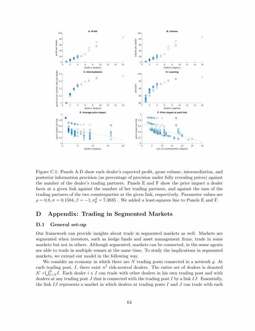
0 2 4 6 8 10 12 14 16
dealer's degrees
0
20
40
60
80
100
prof
it pe
r de
aler
A: Profit
0 2 4 6 8 10 12 14 16
dealer's degrees
0
20
40
60
80
100
volu
me
per
deal
er
B: Volume
0 2 4 6 8 10 12 14 16
dealer's degrees
1
1.1
1.2
1.3
1.4
gros
s-to
-net
vol
ume
ratio
per
dea
ler
C: Intermediation
0 2 4 6 8 10 12 14 16
dealer's degrees
80
85
90
95
100
prec
isio
n
D: Learning
0 5 10 15 20
dealer's degrees
0
0.2
0.4
0.6
0.8
1
pric
e im
pact
per
link
E: Average price impact
0 5 10 15 20 25 30
sum of counterparties' degrees
0
0.2
0.4
0.6
0.8
1
pric
e im
pact
per
link
F: Price impact at each link
Figure C.1: Panels A-D show each dealer’s expected profit, gross volume, intermediation, andposterior information precision (as percentage of precision under fully revealing prices) againstthe number of the dealer’s trading partners. Panels E and F show the price impact a dealerfaces at a given link against the number of her trading partners, and against the sum of thetrading partners of the two counterparties at the given link, respectively. Parameter values areρ = 0.8, σ = 0.1584, β = −1, σ2
θ = 7.3835 . We added a least-squares line to Panels E and F.
D Appendix: Trading in Segmented Markets
D.1 General set-up
Our framework can provide insights about trade in segmented markets as well. Markets aresegmented when investors, such as hedge funds and asset management firms, trade in somemarkets but not in others. Although segmented, markets can be connected, in the sense agentsare able to trade in multiple venues at the same time. To study the implications in segmentedmarkets, we extend our model in the following way.
We consider an economy in which there are N trading posts connected in a network g. Ateach trading post, I, there exist nI risk-neutral dealers. The entire set of dealers is denotedN =
⋃NI=NI. Each dealer i ∈ I can trade with other dealers in his own trading post and with
dealers at any trading post J that is connected with the trading post I by a link IJ . Essentially,the link IJ represents a market in which dealers at trading posts I and J can trade with each
64
other. However, they have access to trade in other markets at the same time. Let gI denotethe set of trading posts that are linked with I in the network g, and mI ≡
∣∣gI ∣∣ represent thenumber of I’s links.
As before, dealers trade a risky asset in zero net supply, and all trades take place at thesame time. Each dealer is uncertain about the value of the asset. In particular, a dealer’svalue for the asset is given by θi, which is a random variable normally distributed with mean0 and variance σ2
θ . Moreover, we consider that values are interdependent across all dealers. Inparticular, V(θi, θj) = ρσ2
θ for any two agents i, j ∈ N . Each dealer receives a private signal,si = θi + εi, where εi ∼ IIDN(0, σ2
ε) and V(θj , εi) = 0, for all i and j.A dealer i ∈ I seeks to maximize her final wealth∑
J∈gIqiIJ(θi − pIJ
),
where qiIJ is the quantity traded by dealer i in market IJ , at a price pIJ . Similarly to the OTCmodel, the trading strategy of the dealer i with signal si is a generalized demand functionQi : Rm
i → Rmi
which maps the vector of prices, pgI = (pIJ)J∈gI , that prevail in the marketsin which dealer i participates in network g into a vector of quantities she wishes to trade
Qi(si; pgI ) =(QiIJ(si; pgI )
)J∈gI
,
where QiIJ(si; pgI ) represents her demand function in market IJ .Apart from trading with each other, dealers also serve a price-sensitive customer base. In
particular, we assume that for each market IJ , the customer base generates a downward slopingdemand
DIJ(pIJ) = βIJpIJ , (D.1)
with an arbitrary constant βIJ < 0. The exogenous demand (D.1) ensures the existence of theequilibrium when agents are risk neutral, and facilitates comparisons with the OTC model.
The expected payoff for dealer i ∈ I corresponding to the strategy profile{Qi(si; pgI
)}i∈N
is
E
∑J∈gI
QiIJ(si; pgI )(θi − pIJ
)|si
where pIJ are the prices for which all markets clear. That is, prices satisfy∑i∈I
QiIJ(si; pgI
)+∑j∈J
QjIJ(sj ; pgJ
)+ βIJpIJ = 0, ∀ IJ ∈ g. (D.2)
D.2 Equilibrium concept
As in the OTC game, we use the concept of Bayesian Nash equilibrium. For completeness, wereproduce it below.
Definition 3 A Linear Bayesian Nash equilibrium of the segmented market game is a vector of
65

linear generalized demand functions{Qi(si; pgI
)}i∈N such that Qi(si; pgI ) solves the problem
max(QiIJ )
J∈gIE
∑J∈gI
QiIJ(si; pgI )(θi − pIJ
) ∣∣si , (D.3)
for each dealer i, where the prices pIJ satisfy (D.2) .
A dealer i chooses a demand function in each market IJ , in order to maximize her expectedprofits, given her information, si, and given the demand functions chosen by the other dealers.
D.3 The Equilibrium
In this section, we outline the steps for deriving the equilibrium in the segmented market gamefor any network structure. First, we derive the equilibrium strategies as a function of posteriorbeliefs. Second, we construct posterior beliefs that are consistent with dealers’ optimal choices.In the OTC game we used the conditional guessing game as an intermediate step in constructingbeliefs. Here, we employ the same line of reasoning, although we do not explicitly introducethe conditional guessing game structure that would correspond to the segmented market game.
D.3.1 Derivation of demand functions
We conjecture an equilibrium in demand functions, where the demand function of dealer i inmarket IJ is given by
QiIJ(si; pgI ) = tIIJ(yIIJsi +
∑K∈gI
zIIJ,IKpIK − pIJ) (D.4)
for any i ∈ I and J . As evident in the notation, we consider that all dealers at trading postI are symmetric in their trading strategy, and weigh in same way the signal they receive andthe prices they trade at. Nevertheless, they end up trading different quantities, as they havedifferent realizations of the signal.
We solve the optimization problem (D.3) pointwise. That is, for each realization of thevector of signals, s, we solve for the optimal quantity qiIJ that each dealer i ∈ I demands inmarket IJ . Given the conjecture (D.4) and the market clearing conditions (D.2), the residualinverse demand function of dealer i in market IJ is
pIJ = −tIIJy
IIJ
∑k∈I,k 6=i
sk + tJIJyJIJ
∑k∈J
sk + (NI − 1)∑
L∈gI ,L 6=JtIIJz
IIJ,ILpIL +NJ
∑L∈gJ ,L 6=I
tJIJzJIJ,JLpJL + qiIJ
(NI − 1) tIIJ
(zIIJ,IJ − 1
)+NJ tJIJ
(zJIJ,IJ − 1
)+ βIJ
.
(D.5)Denote
IJi ≡ −tIIJy
IIJ
∑k∈I,k 6=i
sk + tJIJyJIJ
∑k∈J
sk + (NI − 1)∑
L∈gI ,L6=JtIIJz
IIJ,ILpIL +NJ
∑L∈gJ ,L6=I
tJIJzJIJ,JLpJL
(NI − 1) tIIJ
(zIIJ,IJ − 1
)+NJ tJIJ
(zJIJ,IJ − 1
)+ βIJ
(D.6)
66
and rewrite (D.5) as
pIJ = IJi −1
(NI − 1) tIIJ
(zIIJ,IJ − 1
)+NJ tJIJ
(zJIJ,IJ − 1
)+ βIJ
qiIJ . (D.7)
The uncertainty that dealer i faces about the signals of others is reflected in the random in-tercept of the residual inverse demand, IJi , while her capacity to affect the price is reflected in
the slope −1/(
(NI − 1) tIIJ
(zIIJ,IJ − 1
)+NJ t
JIJ
(zJIJ,IJ − 1
)+ βIJ
). In the segmented mar-
kets game, however, the random intercept IJi reflects not only the signals of the dealers at thetrading post J , but also the signals of the other dealers at the trading post I.
Then, solving the optimization problem (D.3) is equivalent to finding the vector of quantitiesqi = Qi(si; pgI ) that solve
max(qiIJ )
j∈gI
∑J∈gI
qiIJ
E (θi|si,pgI)−IJi − qiIJ
(NI − 1) tIIJ
(zIIJ,IJ − 1
)+NJ tJIJ
(zJIJ,IJ − 1
)+ βIJ
From the first order conditions we derive the quantities qiIJ that dealer i ∈ I trades in eachmarket IJ , for each realization of s, as
21
(NI − 1) tIIJ
(zIIJ,IJ − 1
)+NJ tJIJ
(zJIJ,IJ − 1
)+ βIJ
qiIJ = IJi − E(θi|si,pgI
),
This implies that the optimal demand function
QiIJ(si; pgi) = −((NI − 1) tIIJ
(zIIJ,IJ − 1
)+NJ t
JIJ
(zJIJ,IJ − 1
)+ βIJ
) (E(θi
∣∣si,pgI )− pIJ)
(D.8)for each dealer i in market IJ .
Further, given our conjecture (D.4), equating coefficients in equation (D.8) implies that
E(θi∣∣si,pgI ) = yIIJs
i +∑K∈gI
zIIJ,IKpIK .
However, the projection theorem implies that the belief of each dealer i can be described asa unique linear combination of her signal and the prices she observes. Thus, it must be thatyIIJ = yI , and zIIJ,JK = zIIK for all I, J , and K. In other words, the posterior belief of a dealeri is given by
E(θi∣∣si,pgI ) = yIsi + zgIpgI , (D.9)
where zgI =(zIIJ)J∈gI is a row vector of size mi. Then, we obtain that the trading intensity
of dealer at trading post I satisfies
tIIJ = (NI − 1) tIIJ(1− zIIJ
)+NJ t
JIJ
(1− zJIJ
)− βIJ . (D.10)
If we further substitute this into the market clearing conditions (D.2) we obtain the price
67

in market IJ as follows
pIJ =
tIIJ
(∑i∈I
E(θi|si,pgI
))+ tJIJ
(∑j∈J
E(θj |sj ,pgJ
))NItIIJ +NJ tJIJ − βIJ
. (D.11)
From (D.10) and the analogous equation for tJIJ , it is straightforward to derive the tradingintensity that dealers at trading post I and J have. This implies that we can obtain the pricein each market IJ as
pIJ = wIIJ
(∑i∈I
E(θi|si,pgI
))+ wJIJ
∑j∈J
E(θj |sj ,pgJ
) , (D.12)
where
wIIJ ≡zJIJ − 2
(NJ +NI − 1) zIIJzJIJ − 2 (NI − 1) zIIJ − 2 (NJ − 1) zJIJ − 4
.
This expression is useful to relate the belief of a dealer i ∈ I to the beliefs of other dealers atthe same trading post, and at trading posts that are connected to I.
D.3.2 Derivation of beliefs
We follow the same solution method that we developed in Section 3.1. As before, the key ideais to reduce the dimensionality of the problem and use our conjecture about demand functionsto derive a fixed point in beliefs, instead of the fixed point (D.8).
In the OTC game we constructed each dealer’s equilibrium belief as a linear combinationof the beliefs of her neighbors in the network. For this, we introduced the conditional guessinggame. The conditional guessing game was a useful intermediate step in making the derivationsmore transparent, as well as an informative benchmark about the role of market power for thediffusion of information.
In the segmented market game it is less straightforward to formulate the correspondingconditional guessing game. Since there are multiple dealers at each trading post, it is notimmediate how each dealer forms her guess. In particular, we would need to make additionalassumptions about the linear combination of the guesses of dealers in the same trading postand dealers of the neighboring trading post, that each agent can condition her guess on.
Thus, in the segmented market game we construct beliefs directly as linear combinationsof signals. We conjecture that for each dealer i ∈ I, her belief is an affine combination of thesignals of all dealers in the economy
E(θi|si,pgI
)= vIIIs
i +N∑K=1
vIIKSK , (D.13)
where SK =∑k∈K
sk, ∀K. This further implies that
∑i∈I
E(θi|si,pgI
)= vIIIS
I +NI
N∑K=1
vIIKSK .
68
Before we derive the fixed point equation for beliefs, it is useful to write (D.12) in matrixform, for each trading post I. For this we introduce some more notation. Unless specifiedotherwise, in the notation below we keep I fixed and vary J ∈ {1, ..., N}. Let pI be aN−columnvector with elements pIJ if IJ ∈ g, and 0 otherwise. Let zI be aN−column vector with elementszIIJ if IJ ∈ g, and 0 otherwise. Similarly, let wI be the N−column vector with elements wIIJif IJ ∈ g, and 0 otherwise, while WI be a matrix with elements wJIJ on diagonal if IJ have alink, and 0 otherwise (all elements off-diagonal are 0, as well). Further, let vI be the N−rowvector with elements vIIJ , and vI be the N−row vector with elements vIII at position I and 0otherwise. Let V be the square matrix with rows vI , and V be the matrix with rows vI . LetS be the N−column vector with elements SI . Let N be a square matrix with elements nI ondiagonal and 0 otherwise. Let 1 be the N−column vector of ones.
Substituting our conjecture for beliefs (D.13) in the equation for the price (D.12), we obtainthe vector of prices which dealers at each trading post I are trading as
pI = wI(vI + nIvI
)S +W I
(V + NV
)S.
We are now ready to formalize the result.
Proposition D.1 There exists an equilibrium in the segmented markets game if the followingsystem of equations
vI =(zI)> (
wI(vI + nIvI
)+W I
(V + NV
))1,∀I (D.14)
andvIII = yI , ∀I
admits a solution in vI , for each I.
Proof. As for the OTC game, the proof is constructive. Note that showing that equation(D.14) admits a solution is equivalent to showing that there exists a fixed point in vI . This isbecause, the projection theorem implies that zI , and inherently, wI are a function of vI .
Let vI be a fixed point of (D.14) and vIII = yI , for each I. We construct an equilibrium forthe segmented-market game with beliefs given by (D.13), as follows. We choose convenientlyzI and wI such that
E(θi|si,pgI
)= yIsi +
(zI)> (
wI(vI + nIvI
)+W I
(V + NV
))S
is satisfied. Then, it follows that the prices given by (D.11) and demand functions given by(D.8) is an equilibrium of the OTC game.
The derivation we have outlined above also highlights the main technical difficulty of thesegmented market game relative to the OTC game. That is, the signals of dealers in the sametrading post obscure the (sum of) beliefs of the dealers in neighboring trading posts, such thata dealer can no longer invert the prices she observes and infer what his neighbors posteriors.
D.4 Learning and illiquidity in a star network
In this section, we illustrate the effects of market integration on learning from prices andmarket liquidity in an example.In particular, we restrict ourselves to considering a star network,
69
in which there are nP dealers at each periphery trading post, and nC dealers at the centraltrading post. In particular, we conduct the following numerical exercise. We consider aneconomy with nine agents. Keeping their information set fixed, we compare the following fourmarket structures:
1. 8 trading posts connected in a star network, with one agent in each trading post (N = 8,nP = 1, nC = 1), that is, 8 trading venues. This is our baseline model with a starnetwork.
2. 4 trading posts connected in a star network, with two agents in each periphery node andone agent in the central node (N = 4, nP = 2, nC = 1), that is, 4 trading venues.
3. 2 trading posts connected in a star network, with four agents in each periphery node andone agent in the central node (N = 2, nP = 4, nC = 1), that is, 2 trading venues.
4. A centralized market (N = 1, nP = 9, nC = 0), that is, a single trading venue.
We consider two directions. First, we investigate what drives the illiquidity central and pe-riphery agents face for changing degrees of market segmentation. We concentrate on (il)liquidityas this is a more commonly reported variable in the empirical literature, and we leave the ana-lysis of welfare and expected profits to Appendix D. Second, to complement the analysisin Section 4 , we also analyze how much dealers can learn from prices under these marketstructures.
The left and center panels in Figure D.2 show the average illiquidity that a periphery,1tP
, and a central dealer, 1tC
, face in each of the scenarios described above. We also plot the
average illiquidity that any agent in a centralized market, 1tV
, faces. For easy comparison, allthe parameters are the same as in Section 5.1.
To highlight the intuition, we start with the extreme cases of market segmentation compa-ring illiquidity under a star network and in a centralized market.
D.4.1 Extreme cases of market segmentation with a star network
In this part, we compare illiquidity of dealers in a centralized market and that of a peripheryor central dealer in a star network.
The solid curve in Panels D and the curves in panel F in Figure 2 illustrate that compared toany agent in a centralized market, the central agent in the star faces higher trading price impactin general, but the periphery agents tend to face smaller price impact when the correlationacross values is sufficiently high. We partially prove this result. The following propositionstates that if ρ is sufficiently large, illiquidity for the central agent is larger, while illiquidityfor the periphery agents is lower than that for an agent in a centralized market and, when ρis sufficiently small, illiquidity for any agent in a star network is larger than the illiquidity forany agent in a centralized market.
Proposition D.2
1. When ρ is sufficiently small, such that zV is sufficiently close to 1− 1n−1 , then illiquidity
for any agent in a star network is larger than for any agent in a centralized market
70
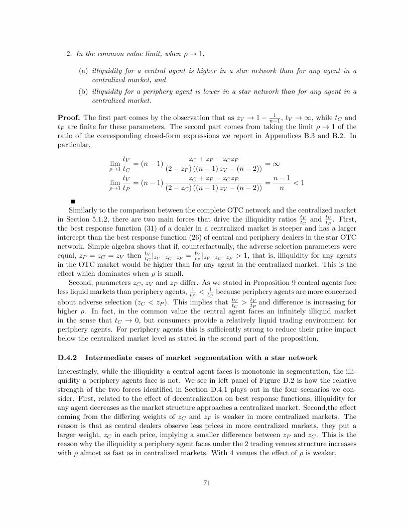
2. In the common value limit, when ρ→ 1,
(a) illiquidity for a central agent is higher in a star network than for any agent in acentralized market, and
(b) illiquidity for a periphery agent is lower in a star network than for any agent in acentralized market.
Proof. The first part comes by the observation that as zV → 1− 1n−1 , tV →∞, while tC and
tP are finite for these parameters. The second part comes from taking the limit ρ → 1 of theratio of the corresponding closed-form expressions we report in Appendices B.3 and B.2. Inparticular,
limρ→1
tVtC
= (n− 1)zC + zP − zCzP
(2− zP ) ((n− 1) zV − (n− 2))=∞
limρ→1
tVtP
= (n− 1)zC + zP − zCzP
(2− zC) ((n− 1) zV − (n− 2))=n− 1
n< 1
Similarly to the comparison between the complete OTC network and the centralized marketin Section 5.1.2, there are two main forces that drive the illiquidity ratios tV
tCand tV
tP. First,
the best response function (31) of a dealer in a centralized market is steeper and has a largerintercept than the best response function (26) of central and periphery dealers in the star OTCnetwork. Simple algebra shows that if, counterfactually, the adverse selection parameters wereequal, zP = zC = zV then tV
tC|zV =zC=zP = tV
tP|zV =zC=zP > 1, that is, illiquidity for any agents
in the OTC market would be higher than for any agent in the centralized market. This is theeffect which dominates when ρ is small.
Second, parameters zC , zV and zP differ. As we stated in Proposition 9 central agents faceless liquid markets than periphery agents, 1
tP< 1
tCbecause periphery agents are more concerned
about adverse selection (zC < zP ). This implies that tVtC
> tVtP
and difference is increasing forhigher ρ. In fact, in the common value the central agent faces an infinitely illiquid marketin the sense that tC → 0, but consumers provide a relatively liquid trading environment forperiphery agents. For periphery agents this is sufficiently strong to reduce their price impactbelow the centralized market level as stated in the second part of the proposition.
D.4.2 Intermediate cases of market segmentation with a star network
Interestingly, while the illiquidity a central agent faces is monotonic in segmentation, the illi-quidity a periphery agents face is not. We see in left panel of Figure D.2 is how the relativestrength of the two forces identified in Section D.4.1 plays out in the four scenarios we con-sider. First, related to the effect of decentralization on best response functions, illiquidity forany agent decreases as the market structure approaches a centralized market. Second,the effectcoming from the differing weights of zC and zP is weaker in more centralized markets. Thereason is that as central dealers observe less prices in more centralized markets, they put alarger weight, zC in each price, implying a smaller difference between zP and zC . This is thereason why the illiquidity a periphery agent faces under the 2 trading venues structure increaseswith ρ almost as fast as in centralized markets. With 4 venues the effect of ρ is weaker.
71
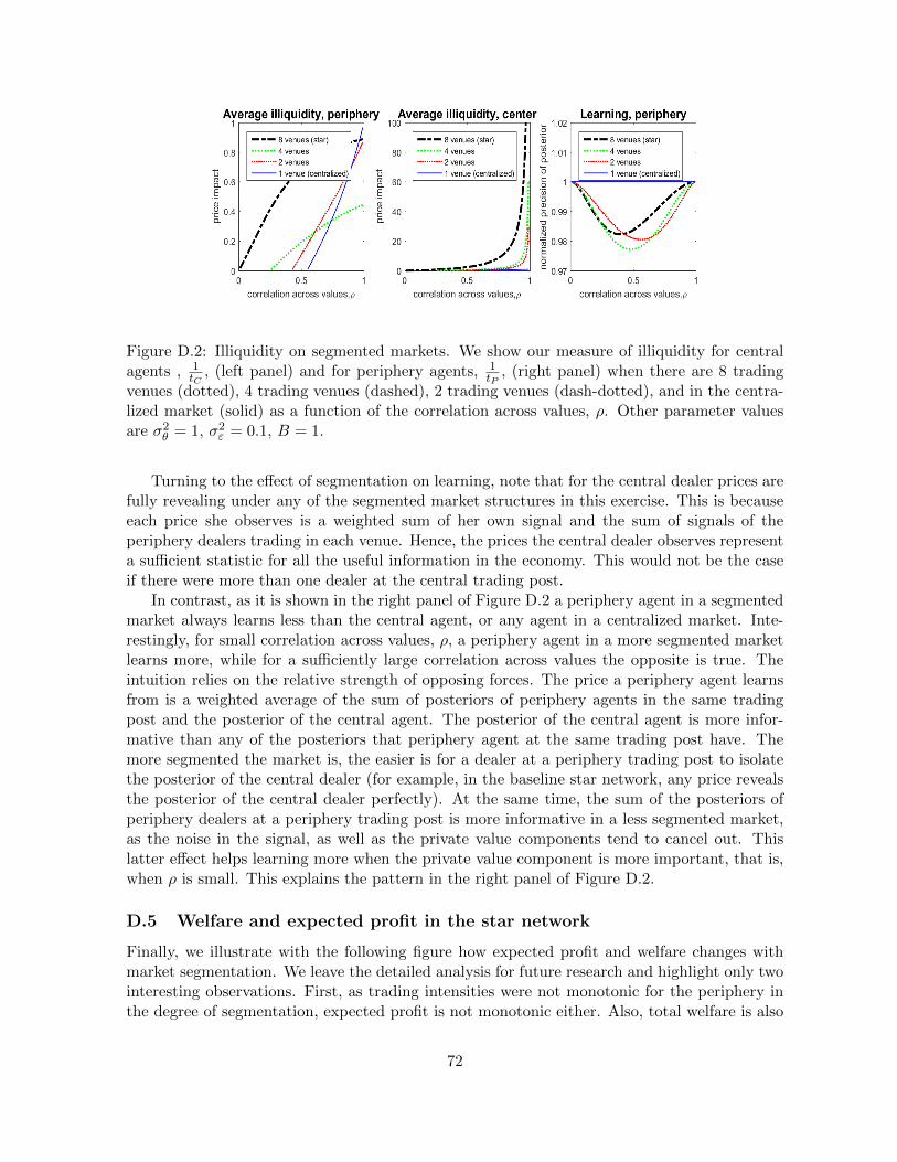
Figure D.2: Illiquidity on segmented markets. We show our measure of illiquidity for centralagents , 1
tC, (left panel) and for periphery agents, 1
tP, (right panel) when there are 8 trading
venues (dotted), 4 trading venues (dashed), 2 trading venues (dash-dotted), and in the centra-lized market (solid) as a function of the correlation across values, ρ. Other parameter valuesare σ2
θ = 1, σ2ε = 0.1, B = 1.
Turning to the effect of segmentation on learning, note that for the central dealer prices arefully revealing under any of the segmented market structures in this exercise. This is becauseeach price she observes is a weighted sum of her own signal and the sum of signals of theperiphery dealers trading in each venue. Hence, the prices the central dealer observes representa sufficient statistic for all the useful information in the economy. This would not be the caseif there were more than one dealer at the central trading post.
In contrast, as it is shown in the right panel of Figure D.2 a periphery agent in a segmentedmarket always learns less than the central agent, or any agent in a centralized market. Inte-restingly, for small correlation across values, ρ, a periphery agent in a more segmented marketlearns more, while for a sufficiently large correlation across values the opposite is true. Theintuition relies on the relative strength of opposing forces. The price a periphery agent learnsfrom is a weighted average of the sum of posteriors of periphery agents in the same tradingpost and the posterior of the central agent. The posterior of the central agent is more infor-mative than any of the posteriors that periphery agent at the same trading post have. Themore segmented the market is, the easier is for a dealer at a periphery trading post to isolatethe posterior of the central dealer (for example, in the baseline star network, any price revealsthe posterior of the central dealer perfectly). At the same time, the sum of the posteriors ofperiphery dealers at a periphery trading post is more informative in a less segmented market,as the noise in the signal, as well as the private value components tend to cancel out. Thislatter effect helps learning more when the private value component is more important, that is,when ρ is small. This explains the pattern in the right panel of Figure D.2.
D.5 Welfare and expected profit in the star network
Finally, we illustrate with the following figure how expected profit and welfare changes withmarket segmentation. We leave the detailed analysis for future research and highlight only twointeresting observations. First, as trading intensities were not monotonic for the periphery inthe degree of segmentation, expected profit is not monotonic either. Also, total welfare is also
72
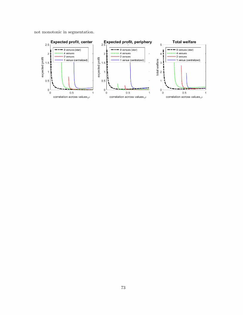
not monotonic in segmentation.
73