topology reconstruction of tree-like structure in images
TRANSCRIPT

Topology Reconstruction of Tree-like Structure in Images via Structural
Similarity Measure and Dominant Set Clustering
Jianyang Xie1, Yitian Zhao1*, Yonghuai Liu2, Pan Su1, Yifan Zhao3*,
Jun Cheng1, Yalin Zheng4, Jiang Liu1
1Ningbo Institute of Industrial Technology
Chinese Academy of Sciences
2Department of Computer Science
Edge Hill University
3School of Aerospace, Transport and Manufacturing
Cranfield University
4Department of Eye and Vision Science
University of Liverpool
Abstract
The reconstruction and analysis of tree-like topological
structures in the biomedical images is crucial for biologists
and surgeons to understand biomedical conditions and plan
surgical procedures. The underlying tree-structure topology
reveals how different curvilinear components are anatomi-
cally connected to each other. Existing automated topology
reconstruction methods have great difficulty in identifying
the connectivity when two or more curvilinear components
cross or bifurcate, due to their projection ambiguity, imag-
ing noise and low contrast. In this paper, we propose a
novel curvilinear structural similarity measure to guide a
dominant-set clustering approach to address this indispens-
able issue. The novel similarity measure takes into account
both intensity and geometric properties in representing the
curvilinear structure locally and globally, and group curvi-
linear objects at crossover points into different connected
branches by dominant-set clustering. The proposed method
is applicable to different imaging modalities, and quantita-
tive and qualitative results on retinal vessel, plant root, and
neuronal network datasets show that our methodology is ca-
pable of advancing the current state-of-the-art techniques.
1. Introduction
Accurate reconstruction of the pervasive tree-like struc-
tures commonly encountered in biomedical imagery, such
as blood vessels in medical images, the roots of plants
in color photography, or neuronal arbors in optical mi-
croscopy images, is a fundamental step in providing valu-
able clinical information in diagnosis of pathological con-
ditions [25, 30], revealing important information about the
delivery of nutrients to different plant tissues [14, 1], or
screening the neuronal connectivity to study the relation be-
tween neuronal structure and function [3, 26], respectively.
In consequence, extracting and representing the geometri-
cal (radii, lengths or tortuosity) and topological (branching
connectivity) properties of these tree-like structures is criti-
cal for diagnosis, or other analytic purposes.
Rapid development has taken place in the automatic ge-
ometric extraction of the properties of tree-like structures,
as evidenced by extensive reviews [16, 32]: but automated
topology reconstruction from a single, two-dimensional (2-
D) image of a three-dimensional (3-D) tree-structure is rel-
atively unexplored, and more challenging. The main reason
is that while a 3-D tree-structure projects readily to a 2-D
image plane, the problem of then reconstructing the topol-
ogy of the tree-like structure from it is ill-posed and error-
prone [14], due to their depth loss in projection, imaging
noise and low contrast in appearance and geometric struc-
tures.
The underlying tree-structure topology must be able to
identify and differentiate individual curvilinear objects from
the entire tree network. The top row of Figure 1 shows ex-
amples of tree-like structures in biomedical imagery: the
bottom row gives their derived topological information.
Manual reconstruction of these tree-structure topologies is
time consuming, and commercial software, e.g., Vaa3D1,
still largely relies on manual annotation and so is subject to
human error [11]. Thus, the catalyst for the development of
algorithms for accurate automatic topology reconstruction
has been primarily the need to overcome time constraints
and avoid human error.
1http://home.penglab.com/proj/vaa3d/home
18505
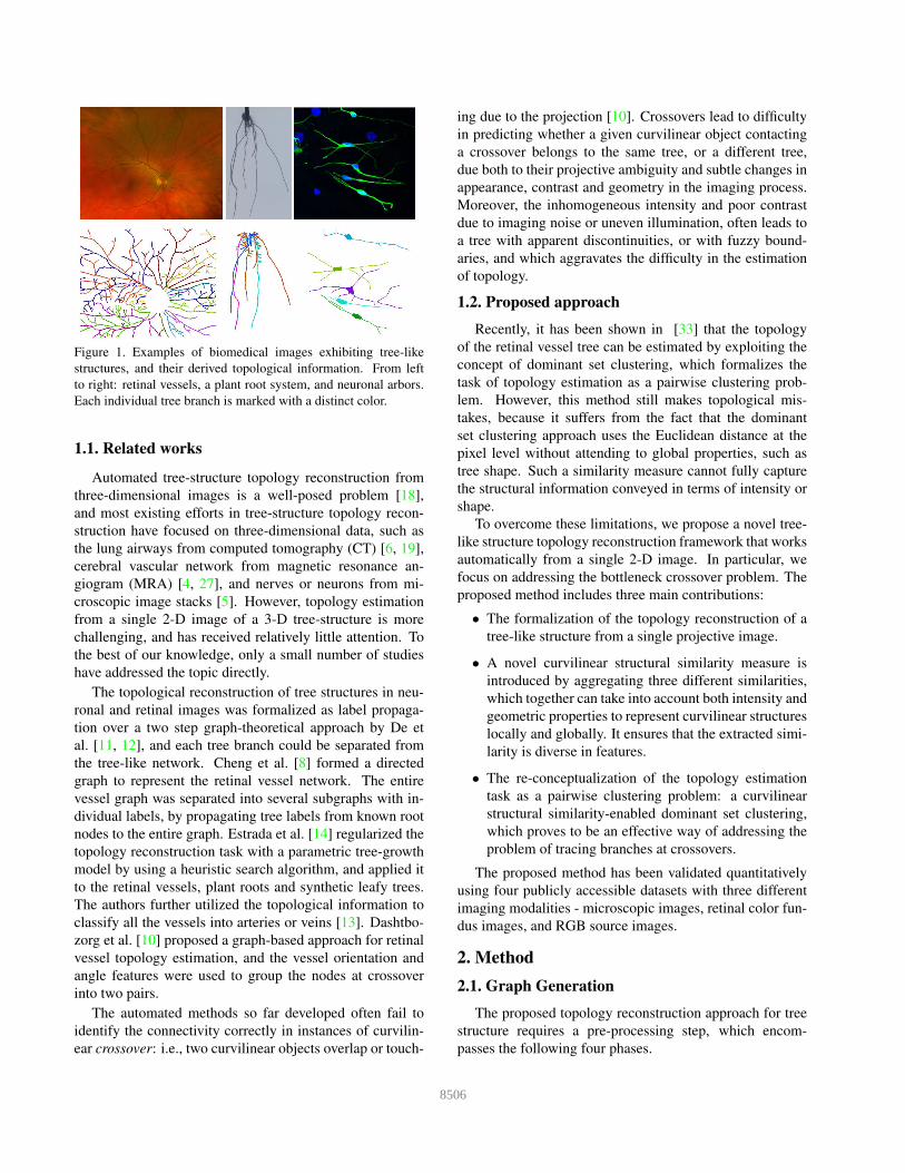
Figure 1. Examples of biomedical images exhibiting tree-like
structures, and their derived topological information. From left
to right: retinal vessels, a plant root system, and neuronal arbors.
Each individual tree branch is marked with a distinct color.
1.1. Related works
Automated tree-structure topology reconstruction from
three-dimensional images is a well-posed problem [18],
and most existing efforts in tree-structure topology recon-
struction have focused on three-dimensional data, such as
the lung airways from computed tomography (CT) [6, 19],
cerebral vascular network from magnetic resonance an-
giogram (MRA) [4, 27], and nerves or neurons from mi-
croscopic image stacks [5]. However, topology estimation
from a single 2-D image of a 3-D tree-structure is more
challenging, and has received relatively little attention. To
the best of our knowledge, only a small number of studies
have addressed the topic directly.
The topological reconstruction of tree structures in neu-
ronal and retinal images was formalized as label propaga-
tion over a two step graph-theoretical approach by De et
al. [11, 12], and each tree branch could be separated from
the tree-like network. Cheng et al. [8] formed a directed
graph to represent the retinal vessel network. The entire
vessel graph was separated into several subgraphs with in-
dividual labels, by propagating tree labels from known root
nodes to the entire graph. Estrada et al. [14] regularized the
topology reconstruction task with a parametric tree-growth
model by using a heuristic search algorithm, and applied it
to the retinal vessels, plant roots and synthetic leafy trees.
The authors further utilized the topological information to
classify all the vessels into arteries or veins [13]. Dashtbo-
zorg et al. [10] proposed a graph-based approach for retinal
vessel topology estimation, and the vessel orientation and
angle features were used to group the nodes at crossover
into two pairs.
The automated methods so far developed often fail to
identify the connectivity correctly in instances of curvilin-
ear crossover: i.e., two curvilinear objects overlap or touch-
ing due to the projection [10]. Crossovers lead to difficulty
in predicting whether a given curvilinear object contacting
a crossover belongs to the same tree, or a different tree,
due both to their projective ambiguity and subtle changes in
appearance, contrast and geometry in the imaging process.
Moreover, the inhomogeneous intensity and poor contrast
due to imaging noise or uneven illumination, often leads to
a tree with apparent discontinuities, or with fuzzy bound-
aries, and which aggravates the difficulty in the estimation
of topology.
1.2. Proposed approach
Recently, it has been shown in [33] that the topology
of the retinal vessel tree can be estimated by exploiting the
concept of dominant set clustering, which formalizes the
task of topology estimation as a pairwise clustering prob-
lem. However, this method still makes topological mis-
takes, because it suffers from the fact that the dominant
set clustering approach uses the Euclidean distance at the
pixel level without attending to global properties, such as
tree shape. Such a similarity measure cannot fully capture
the structural information conveyed in terms of intensity or
shape.
To overcome these limitations, we propose a novel tree-
like structure topology reconstruction framework that works
automatically from a single 2-D image. In particular, we
focus on addressing the bottleneck crossover problem. The
proposed method includes three main contributions:
• The formalization of the topology reconstruction of a
tree-like structure from a single projective image.
• A novel curvilinear structural similarity measure is
introduced by aggregating three different similarities,
which together can take into account both intensity and
geometric properties to represent curvilinear structures
locally and globally. It ensures that the extracted simi-
larity is diverse in features.
• The re-conceptualization of the topology estimation
task as a pairwise clustering problem: a curvilinear
structural similarity-enabled dominant set clustering,
which proves to be an effective way of addressing the
problem of tracing branches at crossovers.
The proposed method has been validated quantitatively
using four publicly accessible datasets with three different
imaging modalities - microscopic images, retinal color fun-
dus images, and RGB source images.
2. Method
2.1. Graph Generation
The proposed topology reconstruction approach for tree
structure requires a pre-processing step, which encom-
passes the following four phases.
28506

(a) (b) (c) (d) (e)Figure 2. The pipeline of the proposed method to reconstruct the topology of tree-like structure from an example image. (a) Tree-like
structure (retinal vessel); (b) Extracted tree-like structure; (c) Skeletonized tree-like structure; (d) Localization of junctions, in which green
triangles indicate bifurcations, red squares and yellow stars crossovers. (e) Reconstructed topology of tree network.
Segmentation: The infinite perimeter active contour
model using hybrid region information [34] was em-
ployed to automatically segment the tree-like structures.
(Note: this step may be skipped for some datasets where
manual annotation of the tree-like structures is provided
with the data source.) Skeletonization: The center-
lines of tree-structures provide an accurate representa-
tion of their topologies. Therefore, an iterative morphol-
ogy thinning operation [2] is performed on the extracted
tree-structures to obtain a single-pixel-wide skeleton map.
Junction localization: The bifurcations, crossovers, and fil-
ament ends (terminal points) may then be extracted from
the skeleton map by locating junction points (pixels with
more than two neighbors) and terminal points (pixels with
one neighbor). All the junction points and their neighbors
are then removed from the skeleton map, producing an im-
age with clearly separated segments. Junctions are catego-
rized into four groups, according to the number of points
involved in each junction - terminal points (1), connecting
points (2), bifurcation points (3), and crossovers/meeting
points (4 and above). The bracketed number indicates the
number of filament segments connected to each intersec-
tion. Graph generation: A graph can be generated from
the skeleton map by linking first and last nodes in the same
segment. The typical misrepresentations from the generated
graph, such as node splitting, missing links and false links,
are corrected by employing a graph modification approach
proposed in [10].
Fig. 2 (a)-(d) shows an example of the outline of the
graph preparation for retinal vessels.
2.2. Dominantset Clustering for Topology Reconstruction
The concept of dominant sets arises from the study
of graph theory, by which a continuous formulation of
the maximum clique problem is defined [23]. An undi-
rected graph G with weighted edges is represented by
G = (V,E, ω), where V is a set of nodes/pixels, edge
set E ⊆ V × V indicates all the possible connections, and
ω : E → R is the positive weight function and represents
the similarity among the pixels in V . A |V |×|V | symmetric
matrix A = (aij) is used to represent the weighted graph Gas an adjacency matrix.
A dominant set can be formally defined based on the
values of similarity among nodes in V . Let S ⊆ V be a
nonempty subset of nodes, pi ∈ V and pj ∈ S. The rela-
tive similarity between pi and pj with respect to the average
similarity between pj and its neighbours in S is defined as:
φS(i, j) = aij −1
|S|
∑
pk∈S
ajk. (1)
The edge weight definition plays a crucial role in the pro-
posed method. In [33], the inverse Euclidean distance be-
tween the two end points of an edge in the feature space is
used, where each node is represented as a 23-dimensional
feature vector. However, this approach lacks of robustness
due to failure to capture global characteristics. In our work,
aij is derived by a curvilinear structural similarity metric
which is aggregated from pixel level, region level, and geo-
metrical similarities. The derivation of this novel similarity
will be proposed below in Sec. 3.
It is known from definition that φS(i, j) in Eqn. (1) can
be either positive or negative. The weight of pi with regard
to S is assigned recursively as:
WS(i) =
{
1 if |S| = 1∑
pj∈S\{pi}
φS\{pi}(i, j)WS\{pi}(j) otherwise.
(2)
where S \{pi} indicates the nodes set S excluding the node
pi, and WS(i) expresses the similarity between node pi and
the nodes of S \ {pi} with respect to the mutual similarity
amongst the nodes in S \ {pi}. Finally, the total weight of
S is calculated by W (S) =∑
pi∈S WS(i).
Formally, a non-empty subset of nodes S, S ⊆ V such
that W (S′) > 0 for any non-empty S′ ⊆ S is said to be a
dominant set if:
WS(i) > 0, for all pi ∈ S (3)
38507

Algorithm 1 Topology Estimation(I)
Inputs: I: a set of points pi that is associated with intersections;
Outputs: S∗: a partition of I , each element of which includes points of the same
branch;
1: initialize the |I| × |I| symmetric matrix A = (aij) by calculating aij =ω(i, j) with respect to given features;
2: S∗ = ∅3: while I 6= ∅ do
4: initialize a |I| dimensional vector x(0) ∈ ∆5: for t = 0 : MaxIteration − 1 do
6: for i = 1 : |I| do
7: x(t+1)i = x
(t)i
(Ax(t))i
x(t)′Ax
(t)
8: end for
9: end for
10: S = ∅11: for each x
(MaxIteration)i > 0 do
12: remove the column and row with respect to pi from A13: S = S
⋃pi
14: end for
15: I = I \ S16: S∗ = S∗
⋃{S}
17: end while
and
WS∪{pi}(i) < 0, for all pi /∈ S. (4)
In general, the weights of edges within the dominant set
of a edge-weighted graph should be large, representing high
internal homogeneity or similarity [23]. By contrast, the
weights of edges which link to the dominant sets externally
will be small. Therefore, the dominant set is a proper so-
lution to identify branches of a tree, because the similarity
of two points from the same branch should be large, while
that of two points belonging to different branches should be
small.
Dominant sets can be identified by local solutions of the
program:
maximize f(x) = x⊤Axsubject to x ∈ ∆,
(5)
where
∆ ={
x ∈ Rd :
d∑
i=1
xi = 1 and xi ≥ 0 for all i = 1, · · · , d}
and d = |I \ S|. A strict local solution x∗ of Eqn. (5) in-
dicates a dominant set S of G, where xi > 0 means that
the node in question pi ∈ S. An effective optimization ap-
proach for solving Eqn. (5) is given by the so-called repli-
cator dynamics [24]:
x(t+1)i = x
(t)i
(Ax(t))i
x(t)⊤Ax(t), (6)
where i = 1, 2, · · · , |S|. It has been proven that for any ini-
tialization of x ∈ ∆, its trajectory will remain in ∆ with the
increase of iteration t. As t in Eqn. (6) increases, the ob-
jective function f(x) in Eqn. (5) is either strictly increasing
or constant. In practice, the stopping criterion of the dy-
namic system can be set as a maximal number of iteration
t, or as a minimal increment of f(x). Algorithm 1 shows
the complete procedure for partitioning a tree structure into
branches S.
It is worth noticing that a peeling-off strategy has been
adopted: i.e., this method iteratively extracts a subset of
points belonging to the same branch (a dominant set S) each
time by using Eqn. (6) and repeating the process with the
remaining points within the intersection I = I \ S. The
identification of different branches at an intersection is car-
ried out by identifying the most obvious branch first, and
then the second most obvious, and so on. Therefore, the
peeling-off strategy is a direct, intuitive implementation of
this procedure [24].
3. Curvilinear structural similarity measure
The similarity metric aij = ω(i, j) in Algorithm 1 is as
yet to be defined. In this section, we will detail this similar-
ity measure.
Traditional similarity measures, such as the Euclidean
distance, cannot fully capture the local and global, or
intensity-based and geometry-based structural information
of the given objects, and it is hard to provide reliable in-
formation for data clustering. Therefore, a fine similarity
measure with informative local and global structural details
is essential in the reconstruction of a complicated tree-like
structure. In this work, we adopt the concept of struc-
tural similarity (SSIM) [29], and re-conceptualize it as a
new tree-structural similarity measurement, which further
exploits the regional and geometric characteristics of curvi-
linear segments.
Two different curvilinear segments will be deemed to
be from the same tree branch if they satisfy the following
anatomical characteristics, which are supported by clinical
and biological evidences [21, 26, 14]:
• High local similarity: their local contrast is small;
• High global similarity: entire objects consist of similar
curvilinear compoenents;
• High geometric similarity: the global orientations and
tortuosity of the curvilinear object are similar.
In consequence, we propose a novel curvilinear struc-
tural similarity measure to satisfy the above properties. This
similarity measurement is aggregated from the similarity
measured at pixel level, region level, and geometrical level.
3.1. Pixelaware structural similarity measure
SSIM is a similarity measure that is able to compare the
local pattern of pixel intensities from the perspective of im-
age formation. Let u and v be the pixel values in the seg-
ments where the nodes pi and pj are located, respectively.
48508

Then the SSIM(i, j) of two segments containing nodes piand pj can be defined as:
SSIM(i, j) =2u′
iv′j
(u′i)2 + (v′
j)2·
2σuiσvj
(σui)2 + (σvj
)2·σuiuj
σuiσvj
.
(7)
The three terms of SSIM are luminance, contrast, and struc-
tural components, respectively [29]. The u′, σu, v′, and
σv are the mean and standard deviation of the pixel values
of the two segments containing nodes pi and pj , respec-
tively, and σuv is the covariance between them. (Note, in
the real application, the size of the two curvilinear segments
are usually in different, as thus they are straightened and re-
sized into a certain shape.) It can be observed that the three
components are relatively independent. For example, the
smaller the difference between u′ and v′, or σu and σv, the
greater the similarity of luminance or contrast. Meanwhile,
the change of luminance or contrast will not affect the struc-
tures measurement. In [29], the structural similarity of two
different objects is equivalent to the correlation coefficient
between u and v, and it is associated with the two normal-
ized vectors (u− u′)/σu and (v − v′)/σv.
3.2. Regionaware structural similarity measure
The pixel level structural similarity measure discussed
above is mainly defined by the intensity values of each
pixel, and so can capture local details of curvilinear objects.
However, a purely pixel level structural similarity measure
cannot well account for regional similarities [9, 15]. There-
fore, in this section, we propose a novel region level struc-
tural similarity measure.
Assume that the given segment i is partitioned into Msuperpixels {pi
m}Mm=1, and segment j is superpixelized
into N patches {pjn}
NM=1 using the Simple Linear Itera-
tive Clustering (SLIC) method. The region-aware structure
similarity (RSIM) of these two segments can be formulated
as:
RSIM(i, j) =
M∑
m=1
N∑
n=1
SSIM(pim,pj
n) · w(pim,pj
n), (8)
where w(pim,pj
n) is a standard Gaussian weighting func-
tion to model the local contrast in terms of geometric dis-
tances between superpixels m and n, so that local contrast
can be effectively combined with control over the influence
radius:
w(pim,pj
n) =1
Zexp{−
‖pim − pj
n‖2
2σ2}, (9)
where Z is the normalization term to ensure that∑N
n=1,n 6=m w(pim,pj
n) = 1. The range of the regional sim-
ilarity may be controlled by the standard deviation σ2 from
0 to 1. Larger values of σ increase the spatial weighting of
the distant segments, and vice versa. In our implementation,
we set σ2 = 0.3 empirically. The operator ‖ ·‖ indicates the
spatial distance between pim and pj
n.
The RSIM considers not only the local intensity values,
but also how the pixel values are distributed in each patch,
and how similar such distributions are between different
patches. This method treats patches (superpixels) instead as
units for similarity measurement by considering how sim-
ilar different patches are and comparing them directly to
each other [15] in order to determine their relative contrast
and similarity.
3.3. Geometryaware structural similarity measure
Dividing the intensity-based structural similarity into
pixel level and region level, helps in obtaining the object
structural similarity. However, in the field of biomedical im-
age analysis, the object’s shape or geometry level similarity
is crucial to revealing abnormalities [35]. To this end, we
propose a novel geometrical structural similarity measure
(GSIM) in this work. This GSIM can capture the overall
geometry of a shape, or the tortuosity of a curvilinear com-
ponent, and is more robust to variation in imaging quality
and scale.
In our work, the shape index is proposed in order to cap-
ture the intuitive notion of ‘shape’ locally and globally [20].
The shape index E of each centerline pixel in a given seg-
ment may be defined as
E =2
πarctan
C2 + C1
C2 − C1, (10)
where C1 and C2 are the curvatures of each side of a curvi-
linear segment. The curvature obtained from eigensystem
analysis of the Hessian matrix is commonly used in the
computation of vectors tangent to oriented structures [31].
The measurement of shape index in a 3D surface is better
able to represent the concavity or convexity of a given re-
gion, and in 2D or 1D applications, it may be employed to
reveal the global tortuosity of a given shape or curve.
The GSIM can be obtained by calculating the relative
distance between their arguments:
GSIM(i, j) = exp{
−rd(E ′
i ,E′j )
2
2g2}
, (11)
where E ′ indicates the mean shape index value of a seg-
ment, and g is a control parameter that is able to reveal how
distant pixels and dissimilar features will impact the shape
index of the current pixel: here, g2 = 3 is empirically cho-
sen. The relative distance rd(·) of two shape indices be-
tween two objects is defined as:
rd(Ei,Ej) =‖Ei,Ej‖
avek⊂S(‖Ei,Ej‖), (12)
58509

(a) Origin (b) Groundtruth (c) LBP (d) MMNX (e) MFTD (f) Ours
Figure 3. Two examples of topology reconstruction by different methods on neuron arbors from the NeurB1 and NeurB2 dataset.
Table 1. Performances of different methods in identifying the connectivity at junctions, and their DIADEM scores for the NeurB1 and
NeurB2 datasets.
Dataset # Junction Method# Correctly
AccI AccII DIADEMIdentified
NeurB1 557
Ours 501 90.0% 93.6% 0.67
LBP - - - 0.42
MFTD 389 69.8% - 0.52
MMNX 207 37.2% - 0.43
NeurB2 254
Ours 207 81.5% 92.0% 0.63
LBP - - - 0.19
MFTD 199 78.4% - 0.26
MMNX 67 26.4% - 0.22
where avek⊂S(‖Ei − Ej‖) is the average Euclidean dis-
tance of shape index values between segment i and other
candidate segment k in intersection S.
3.4. Similarity Fusion via OWA aggregation
Each of the three aforementioned curvilinear structural
similarity measures has disadvantages if used alone in real
applications. However, they can be aggregated to provide
a more robust solution. Weighted average operators (linear
summation, Hadamard product, average operator, etc.) are
commonly used to implement the aggregation process. In
this work, we formulate a combined curvilinear structural
similarity by using an Ordered Weighted Averaging (OWA)
operator to combat the scale and illumination change from
one segment to another.
The fundamental aspect of an OWA operator is the rank-
ing step, in which the extraneous variables are ranked in
descending order, with their values subsequently integrated
into a single aggregated value [28]. An OWA mapping
AOWA: Rq → R is defined as
AOWA(a1, · · · , aQ) =
Q∑
q=1
wqaπ(q), (13)
where aπ(q) is a permutation of aq , in which aπ(q) is the q-
th largest value of the aq . The ordering of input arguments
gives the OWA a nonlinear character. wq is a collection of
weights that satisfies∑
q wq = 1, q = 1, · · · , Q,Q > 1.
Different choices of the weight w lead to different aggre-
gation results: in our work, w1 = 0.25, w2 = 0.35, and
w3 = 0.4 were chosen empirically. By applying the OWA
aggregation to a real problem of this kind, users will have
the degree of freedom to control both the t-transitivity of the
operator [28], by tuning the stress function, or by tuning the
weights in a weighting vector.
4. Datasets and Experimental Results
4.1. Datasets
Four tree-like image datasets were used in this work
to validate the effectiveness of our approach: two neu-
ronal image datasets (NeuB1 and NeuB2 [11] ), one reti-
nal image dataset (WIDE [14]), and one plant root dataset
(RICE [14]).
The neuronal datasets NeuB1 and NeuB2 contain 112
and 98 neuronal images, respectively. (Note: images from
the NeuB2 dataset are more challenging, due to noise and
blurring.) The manual annotations of structure topology
were made by using the annotation tool Neuromantic2.
The WIDE dataset [14] comprises 15 high resolution
color fundus images, each of 3900×3072 pixels. The RICE
dataset [14] comprises of 18 rice-root RGB source images
of 1300×900 pixels. Both datasets are available from Duke
University, and the manual annotations of the topological
2https://www.reading.ac.uk/neuromantic/body_
index.php
68510

trees were generated by a sketching software [7].
4.2. Results on NeurB1 and NeurB2 datasets
Figure 3 presents for visual comparison the topology
reconstruction results of the competing methods on two
example images from the NeurB1 and NeurB2 neuronal
dataset: a commercially available neurite tracer module
of Metamorph NX (MMNX)3; and two label propagation
methods for tree-structure topology estimation: Loopy Be-
lief Propagation (LBP) [22], and Matrix Forest Theorem of
Directed (MFTD) [11]. Pink discs indicate incorrectly iden-
tified junctions, and gray square demonstrate correctly iden-
tified junctions of neuronal images. Compared with their
gold standards, it is clear from visual inspection that the
proposed method made consistently far fewer mistakes.
To facilitate better observation and objective evaluation
of the performance of the proposed method in the topology
reconstruction of tree-like structures, we calculate the accu-
racy of the identified junctions and their associated curvilin-
ear centerline pixels of the tree-like structure as follows. Let
A be the total number of the junctions or centerline pixels
of a tree-like structure, and B be the number of the junc-
tions or centerline pixels that have been correctly identified
(the vertices of the estimated topology tree have been as-
signed labels identical with groundtruth). The accuracy is
then computed by Acc = BA× 100%, and here we refer to
AccI and AccII as the accuracy at junction level, and cen-
terline pixel level, respectively. In addition, the DIADEM
score [17] is utilized to measure the similarity between a
groundtruth tree-like structure and the corresponding topol-
ogy estimation result. The DIADEM score is a widely-used
metric to measure the similarity of two neuronal structures,
and the obtained score falls in the range [0, 1], where 0 indi-
cates a completely mismatch and 1 indicates perfect agree-
ment. The x-y threshold of the DIADEM score is set as 30
pixels in this experiment.
Table 1 presents the performance measurements of the
proposed method and competing methods in identifying
connectivity at junctions. It may be observed that the pro-
posed method is able to detect the most of the junctions cor-
rectly, with AccI = 90.0%, AccII = 93.6%, and DIADEM
score = 0.67 in the NeurB1 dataset. Overall, our approach
consistently outperforms the commercial software and the
other topology estimation methods by a rather large margin
with respect to crossover issues. (Note: we quote the visual
and numerical results reported in [11] in the belief that their
results were the best achievable.)
3https://www.moleculardevices.com/
en/assets/tutorials-videos/dd/img/
introduction-metamorph-nx-software
Table 2. Performances of the proposed method in identifying con-
nectivity at junctions from the WIDE and RICE datasets.
Dataset # Junction# Correctly
AccI AccIIIdentified
WIDE 4908 4743 96.6% 93.6%
RICE 962 949 98.7% 98.9%
Table 3. Topology reconstruction performances of different meth-
ods from the WIDE and RICE datasets.Dataset Method sp sf sa sr
WIDE
Human 0.988 0.991 0.826 0.940
Ours 0.971 0.980 0.788 0.901
HSA 0.966 0.972 0.732 0.860
GLA 0.906 0.920 0.571 0.748
RICE
Ours 0.988 0.992 0.921 0.984
HSA 0.983 0.991 0.898 0.972
GLA 0.941 0.958 0.795 0.895
4.3. Results on the WIDE and RICE datasets
Figures 4 and 5 illustrate the topology reconstruction re-
sults on the WIDE and RICE datasets. Again, we first mea-
sure the performance of the proposed method in identifying
connectivity in the WIDE and RICE datasets, as shown in
Table 2, by counting the number of correctly identified junc-
tions. As expected, the accuracy of the topology reconstruc-
tion at vessel centerline level (i.e. AccII = 93.6% in WIDE
dataset) is lower than the result obtained at junction level
(AccI = 96.6%). This is because the number of curvilinear
segments is much larger than the number of junctions.
In order to provide an objective evaluation, we have com-
pared the proposed method with a Heuristic Search Algo-
rithm (HSA) [14] that efficiently explores the space of pos-
sible trees starting from the Greedy Linear-time Algorithm
(GLA) [14], and these are the only two methods in the lit-
erature that have reported topology reconstruction perfor-
mances on these two datasets. For the sake of fair compari-
son, four weighted scores were obtained to measure the sim-
ilarity between each reconstructed tree and the ground-truth
tree: parent similarity (sp), flow similarity (sf), absolute sim-
ilarity (sa), and relative similarity (sr). The first two demon-
strate local performance in connectivity, while the latter two
capture more global differences. For more detail, we refer
the reader to [14].
Table 3 reports the comparison of our method with
the state-of-the-art topology reconstruction methods on the
WIDE and RICE datasets. For the WIDE dataset, the inter-
observer scores were reported in [14]. It can be seen that
the similarity scores of the proposed method are very close
to those of the human observer. All three methods - the
proposed method and its two competitors - achieve superior
performances on the RICE dataset. That is because the roots
of rice plants have fewer branches than the other datasets,
and these root structures have a tendency to grow down-
wards through the ground (right direction of Figure 5), giv-
78511

(a) Origin (b) Groundtruth (c) HSA (d) OursFigure 4. Two examples of topology reconstruction by different methods on retinal vessels from the WIDE dataset. The white circles
indicate the incorrectly identified junctions.
(a) Origin (b) Groundtruth (c) HSA (d) Ours
Figure 5. Two examples of topology reconstruction by different methods on plant roots from the RICE dataset.
ing a radially symmetrical appearance. In consequence, the
less variable images tend to lead to more accurate results in
the topology estimation task.
5. Conclusions
The topology reconstruction from a single 2-D image
of a 3-D tree-structure is challenging, since the full spa-
tial location of each tree branch is lost after projection. In
this paper, we have proposed a novel topology estimation
method for tree-like structures, formulated as a pairwise
clustering problem. First, a novel curvilinear structure sim-
ilarity measurement is proposed, then it is utilized to guide
the dominant-set clustering approach to identify the connec-
tivity at the junctions, before finally achieving an accurate
topology estimation of the tree network.
It is worth noting that by using this method the number
of points processed in the course of identifying a dominant
set is greatly reduced, from the number of pixels in an image
to the number of junctions in a tree network. This leads to
an increase of time-efficiency in topology estimation. The
competitiveness of our approach is demonstrated by the fact
that it accurately reconstructed tree topologies from four
publicly accessible biomedical image datasets with differ-
ent imaging modalities. The results demonstrated that our
method achieves superior performances when compared di-
rectly with the existing state-of-the-art ones. It is believed
that the proposed method could be a powerful tool for ana-
lyzing tree-like structures in the biomedical images.
6. Acknowledgments
This work was supported by National Science Foun-
dation Program of China (61601029), Zhejiang Provincial
Natural Science Foundation (LZ19F010001), and Ningbo
Natural Science Foundation (2018A610055).
References
[1] L. Band et al. Multiscale systems analysis of root growth
and development: Modeling beyond the network and cellular
scales. The Plant Cell Online, 24(10):3892–3906, 2012. 1
88512
[2] P. Bankhead, J. McGeown, and T. Curtis. Fast retinal vessel
detection and measurement using wavelets and edge location
refinement. PLoS ONE, 7:e32435, 2009. 3
[3] S. Basu et al. Neurite tracing with object process. IEEE
Trans. Med. Imaging, 35(6):1443–1451, 2016. 1
[4] H. Bogunovic et al. Anatomical labeling of the circle of
willis using maximum a posteriori probability estimation.
IEEE Trans. Med. Imag., 32(9):1587–1599, 2013. 2
[5] K. Brown et al. The DIADEM data sets: Representative light
microscopy images of neuronal morphology to advance au-
tomation of digital reconstructions. Neuroinformatics, 9(2-
3):143–157, 2011. 2
[6] J. P. Carson, D. R. Einstein, and R. A. Corley. High res-
olution lung airway cast segmentation with proper topology
suitable for computational fluid dynamic simulations. Comp.
Med. Imag. and Graph., 34(7):572–578, 2010. 2
[7] X. Chen et al. Sketch-based tree modeling using markov
random field. ACM Trans. Graph., 27(5):109:1–109:9, 2008.
7
[8] L. Cheng, J. De, X. Zhang, F. Lin, and H. Li. Tracing retinal
blood vessels by matrix-forest theorem of directed graphs. In
Medical Image Computing and Computer-Assisted Interven-
tion - MICCAI 2014, pages 626–633, 2014. 2
[9] M. Cheng et al. Global contrast based salient region detec-
tion. IEEE Trans. Pattern Anal. Mach. Intell., 37(3):569–
582, 2015. 5
[10] B. Dashtbozorg et al. An automatic graph-based approach
for artery/vein classification in retinal images. IEEE Trans.
Image Processing, 23(3):1073–1083, 2014. 2, 3
[11] J. De et al. A graph-theoretical approach for tracing filamen-
tary structures in neuronal and retinal images. IEEE Trans.
Med. Imaging, 35(1):257–72, 2016. 1, 2, 6, 7
[12] J. De et al. Transduction on directed graphs via absorb-
ing random walks. IEEE Trans. Pattern Anal. Mach. Intell.,
40(7):1770–1784, 2018. 2
[13] R. Estrada and et al. Retinal artery-vein classification
via topology estimation. IEEE Trans. Med. Imaging,
34(12):2518–2534, 2015. 2
[14] R. Estrada et al. Tree topology estimation. IEEE Trans.
Pattern Anal. Mach. Intell., 37(8):1688–1701, 2015. 1, 2, 4,
6, 7
[15] D. Fan et al. Structure-measure: A new way to evaluate fore-
ground maps. In IEEE International Conference on Com-
puter Vision, ICCV 2017, pages 4558–4567, 2017. 5
[16] M. Fraz and et al. Blood vessel segmentation methodolo-
gies in retinal images - a survey. Comput. Meth. Prog. Bio.,
108:407–433, 2012. 1
[17] T. A. Gillette, K. M. Brown, and G. A. Ascoli. The DI-
ADEM metric: Comparing multiple reconstructions of the
same neuron. Neuroinformatics, 9(2-3):233–245, 2011. 7
[18] P. Glowacki et al. Reconstructing evolving tree structures in
time lapse sequences by enforcing time-consistency. IEEE
Trans. Pattern Anal. Mach. Intell., 40(3):755–761, 2018. 2
[19] R. Grothausmann et al. Method for 3d airway topol-
ogy extraction. Comp. Math. Methods in Medicine,
2015:127010:1–127010:7, 2015. 2
[20] J. J. Koenderink. Solid shape. MIT Press, 1990. 5
[21] A. Mosinska-Domanska et al. Active learning for delineation
of curvilinear structures. In IEEE Conference on Computer
Vision and Pattern Recognition, CVPR 2016, pages 5231–
5239, 2016. 4
[22] K. P. Murphy, Y. Weiss, and M. I. Jordan. Loopy belief prop-
agation for approximate inference: An empirical study. In
Proc. ICUAL, pages 467–475, 1999. 7
[23] M. Pavan and M. Pelillo. Dominant sets and hierarchical
clustering. In IEEE International Conference on Computer
Vision (ICCV 2003),, pages 362–369, 2003. 3, 4
[24] M. Pavan and M. Pelillo. Dominant sets and pairwise cluster-
ing. IEEE Trans. Pattern Anal. Mach. Intell., 29(1):167–172,
2007. 4
[25] T. Qureshi and B. Al-Diri. A bayesian framework for the
local configuration of retinal junctions. In IEEE Conference
on Computer Vision and Pattern Recognition, CVPR 2014,
pages 3105–3110, 2014. 1
[26] M. Radojevic and E. Meijering. Automated neuron tracing
using probability hypothesis density filtering. Bioinformat-
ics, 33(7):1073–1080, 2017. 1, 4
[27] D. Robben and et al. Simultaneous segmentation and
anatomical labeling of the cerebral vasculature. Medical Im-
age Analysis, 32:201–215, 2016. 2
[28] P. Su et al. Exploiting data reliability and fuzzy clustering for
journal ranking. IEEE Trans. Fuzzy Systems, 25(5):1306–
1319, 2017. 6
[29] Z. Wang et al. Image quality assessment: from error visibil-
ity to structural similarity. IEEE Trans. Image Processing,
13(4):600–612, 2004. 4, 5
[30] J. Xie, Y. Zhao, and Y. Wang. Retinal vascular topology es-
timation via dominant sets clustering. In IEEE International
Symposium on Biomedical Imaging, ISBI 2018, pages 1458–
1462, 2018. 1
[31] J. Zhang et al. Reconnection of interrupted curvilinear struc-
tures via cortically inspired completion for ophthalmologic
images. IEEE Trans. Biomed. Engineering, 65(5):1151–
1165, 2018. 5
[32] Y. Zhao et al. Automatic 2D/3D vessel enhancement in
multiple modality images using a weighted symmetry filter.
IEEE Trans. Med. Imaging, pages 1–1, 2017. 1
[33] Y. Zhao et al. Retinal artery and vein classification via dom-
inant sets clustering-based vascular topology estimation. In
International Conference on Medical Image Computing and
Computer Assisted Intervention - MICCAI 2018, pages 56–
64, 2018. 2, 3
[34] Y. Zhao, S. P. Harding, and Y. Zheng. Automated vessel seg-
mentation using infinite perimeter active contour model with
hybrid region information with application to retinal images.
IEEE Trans. Med. Imaging, 34(9):1797–1807, 2015. 3
[35] Y. Zhao, Y. Zheng, Y. Liu, J. Yang, Y. Zhao, and Y. Wang.
Intensity and compactness enabled saliency estimation for
leakage detection in diabetic and malarial retinopathy. IEEE
Trans. Med. Imaging, 36(1):51–63, 2017. 5
98513