1 dan graur methods of tree reconstruction. 2 3
TRANSCRIPT

1
Dan Graur
Methods of Methods of Tree Tree
ReconstructionReconstruction

2

3

4

5

6
Molecular phylogenetic approaches:
1. distance-matrix (based on distance measures)
2. character-state (based on character states)
3. maximum likelihood (based on both character states and distances)

7
DISTANCE-MATRIX METHODS
In the distance matrix methods, evolutionary distances (usually the number of nucleotide substitutions or amino-acid replacements between two taxonomic units) are computed for all pairs of taxa, and a phylogenetic tree is constructed by using an algorithm based on some functional relationships among the distance values.

8
GCGGCTCA TCAGGTAGTT GGTG-G SpinachGCGGCCCA TCAGGTAGTT GGTG-G RiceGCGTTCCA TC--CTGGTT GGTGTG MosquitoGCGTCCCA TCAGCTAGTT GTTG-G MonkeyGCGGCGCA TTAGCTAGTT GGTG-A Human*** ** * * *** * **
Multiple AlignmentMultiple Alignment

9
Compute pairwise distances Compute pairwise distances by correcting for multiple by correcting for multiple hits at a single siteshits at a single sites
Number of differences Number of differences
Number of changes (e.g., number of Number of changes (e.g., number of nucleotide substitutions, number of nucleotide substitutions, number of amino acid replacements)amino acid replacements)

10
Distance Matrix**
Spinach Rice Mosquito Monkey HumanSpinach 0.0 9 106 91 86
Rice 0.0 118 122 122
Mosquito 0.0 55 51
Monkey 0.0 3
Human 0.0
**Units: Numbers of nucleotide substitutions per 1,000 nucleotide sites

11
Distance Methods:
UPGMA
Neighbor-relations
Neighbor joining

12
UPGMA UPGMA Unweighted pair-group method with Unweighted pair-group method with
arithmetic meansarithmetic means

13
UPGMA employs a sequential clustering algorithm, in which local topological relationships are identified in order of decreased similarity, and the tree is built in a stepwise manner.

14
simple OTUs

15
composite OTU

16

17

18
UPGMA yields the correct answer only if the distances are ultrametric!
Q: What happens if the distances are only additive?
Q: What happens if the distances are not even additive?

19
Neighborliness methods
The neighbors-relation
method (Sattath & Tversky)
The neighbor-joining method (Saitou & Nei)

20
In an unrooted bifurcating tree, two OTUs are said to be neineigghborshbors if they are connected through a single internal node.
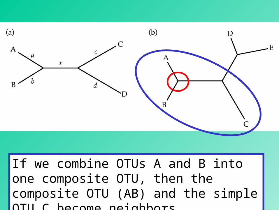
21
If we combine OTUs A and B into one composite OTU, then the composite OTU (AB) and the simple OTU C become neighbors.

A
B
C
D
+ < + = +
Four-Point Conditiond(A,B)+d(C,D)<d(A,C)+d(B,D) =d(A,D)+d(B,C)

23
The Neighbor Joining Method

24
In distance-matrix methods, it is assumed:
SimilaritySimilarity KinshipKinship

25

26
Similarities among OTUs can be due to:
• Ancestry:– Shared ancestral characters (symplesiomorphies)
– Shared derived characters (synapomorphy)• Homoplasy:
– Convergent events – Parallel events– Reversals
From Similarity to From Similarity to RelationshipRelationship

27
Parsimony Methods:
Willi HennigWilli Hennig1913-19761913-1976
28
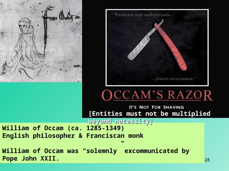
William of Occam (ca. 1285-1349)English philosopher & Franciscan monk
William of Occam was “solemnly” excommunicated by Pope John XXII.
[Entities must not be multiplied [Entities must not be multiplied beyond necessity]beyond necessity]

29
MAXIMUM PARSIMONY METHODS
Maximum parsimony involves the identification of a topology that requires the smallest number of evolutionary changes to explain the observed differences among the OTUs under study.
In maximum parsimony methods, we use discrete character states, and the shortest pathway leading to these character states is chosen as the “best” or maximum parsimony tree.
Often two or more trees with the same minimum number of changes are found, so that no unique tree can be inferred. Such trees are said to be equally parsimonious.
30
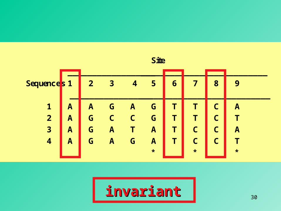
Site
____________________________________________
Sequences 1 2 3 4 5 6 7 8 9
____________________________________________
1 A A G A G T T C A
2 A G C C G T T C T
3 A G A T A T C C A
4 A G A G A T C C T* * *
invariantinvariant

31
Site
____________________________________________
Sequences 1 2 3 4 5 6 7 8 9
____________________________________________
1 A A G A G T T C A
2 A G C C G T T C T
3 A G A T A T C C A
4 A G A G A T C C T* * *
variantvariant

32
Site
____________________________________________
Sequences 1 2 3 4 5 6 7 8 9
____________________________________________
1 A A G A G T T C A
2 A G C C G T T C T
3 A G A T A T C C A
4 A G A G A T C C T* * *
uninformativeuninformative

33
Site
____________________________________________
Sequences 1 2 3 4 5 6 7 8 9
____________________________________________
1 A A G A G T T C A
2 A G C C G T T C T
3 A G A T A T C C A
4 A G A G A T C C T* * *
informativeinformative

34

35

36

37

38
In the case of four OTUs, an informative site can only favor one of the three possible alternative trees.
Thus, the tree supported by the largest number of informative sites is the most parsimonious tree.

39
Inferring the maximum Inferring the maximum parsimony tree:parsimony tree:
1. Identify all the informative sites. 2. For each possible tree, calculate the minimum number of substitutions at each informative site. 3. Sum up the number of changes over all the informative sites for each possible tree.4. Choose the tree associated with the smallest number of changes as the maximum parsimony tree.
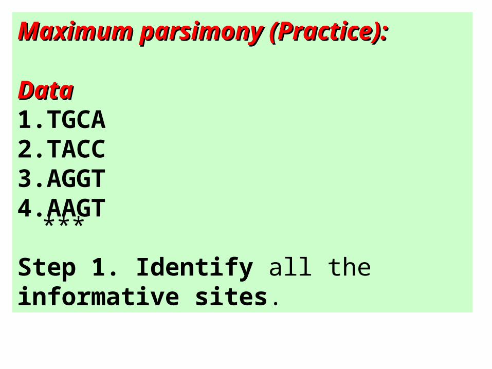
Maximum parsimony (Practice):Maximum parsimony (Practice):
DataData1.TGCA2.TACC3.AGGT4.AAGT
Step 1. Identify all the informative sites.
***

41
Maximum parsimony (Practice):Maximum parsimony (Practice):
DataData1.TGC2.TAC3.AGG4.AAG
Step 2. For each possible tree, calculate the minimum number of substitutions at each informative site.

42
Maximum parsimony (Practice):Maximum parsimony (Practice):
DataData1.TGC2.TAC3.AGG4.AAG
Step 3. Sum up the number of changes over all the informative sites for each possible tree.
4
5
6

43
Maximum parsimony (Practice):Maximum parsimony (Practice):
DataData1.TGC2.TAC3.AGG4.AAG
Step 4. Choose the tree associated with the smallest number of changes as the maximum parsimony tree.
4
5
6

44
Problem (exaggerated)Problem (exaggerated)

45
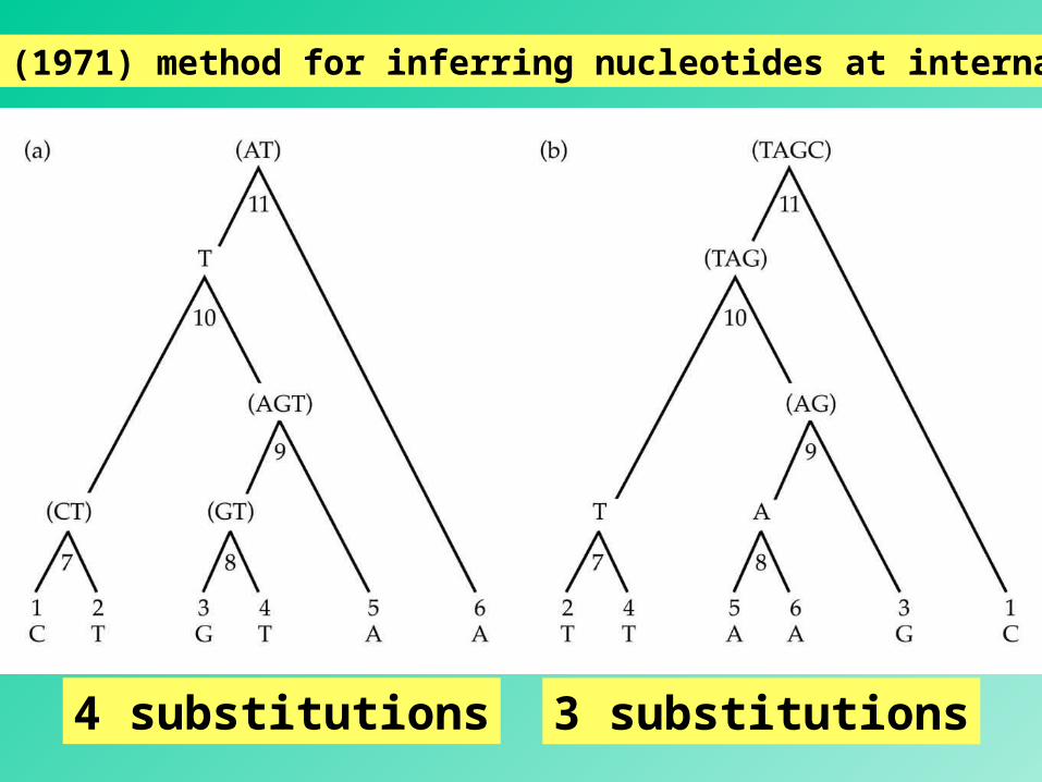
Fitch’s (1971) method for inferring nucleotides at internal nodes
The set at an internal node is the intersection () of the two sets at its immediate descendant nodes if the intersection is not empty.
The set at an internal node is the union (of the two sets at its immediate descendant nodes if the intersection is empty.
When a union is required to form a nodal set, a nucleotide substitution at this position must be assumed to have occurred.
46
Fitch’s (1971) method for inferring nucleotides at internal nodes
4 substitutions 3 substitutions

47
Testing properties of ancestral proteins
The ability to infer in silico the sequence of ancestral proteins, in conjunction with some astounding developments in synthetic biology, allow us to “resurrect” putative ancestral proteins in the laboratory and test their properties. These properties, in turn, can be used to test hypotheses concerning the physical environment which the ancestral organism inhabited (its paleoenvironment).
48
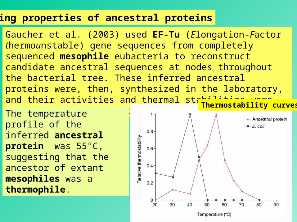
Testing properties of ancestral proteins
Gaucher et al. (2003) used EF-Tu (Elongation-Factor thermounstable) gene sequences from completely sequenced mesophile eubacteria to reconstruct candidate ancestral sequences at nodes throughout the bacterial tree. These inferred ancestral proteins were, then, synthesized in the laboratory, and their activities and thermal stabilities were measured and compared to those of extant organisms.
Thermostability curves The temperature profile of the inferred ancestral protein was 55°C, suggesting that the ancestor of extant mesophiles was a thermophile.

49
Ancestral reconstruction is not possible with morphological data.

50
________________________________________________Number of OTUs Number of possible rooted tree________________________________________________
2 13 34 15
5 1056 954
7 10,3958 135,1359 2,027,025
10 34,459,42515 213,458,046,676,87520 8,200,794,532,637,891,559,375
________________________________________________
The impossibility of exhaustively searching for the maximum-parsimony tree when the number of OTUs is large

51
Exhaustive = Examine allall trees, get the bestbest tree (guaranteed).
Branch-and-Bound = Examine somesome trees, get the bestbest tree (guaranteed).
Heuristic = Examine some trees, get a tree that may may or may not be or may not be the bestbest tree.

52
Exhaustive
53
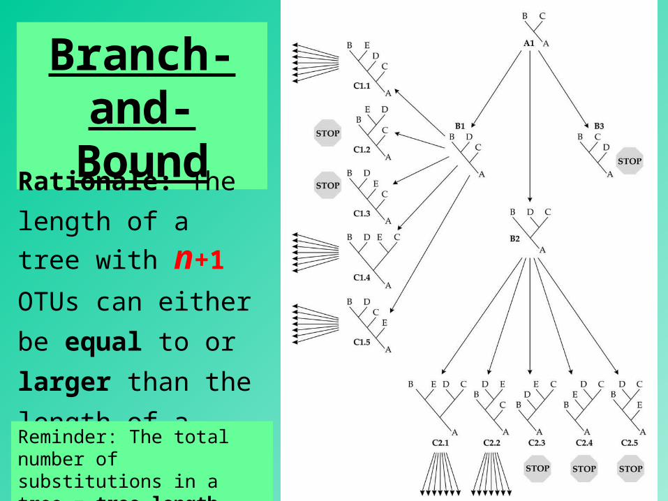
Branch-and-BoundRationale: The
length of a
tree with n+1 OTUs can either
be equal to or
larger than the
length of a
tree with n OTUs.
Reminder: The total number of substitutions in a tree = tree length

54
Branch-and-Bound
Obtain a tree by a fast method. (e.g., the neighbor-joining method)
Compute numbers of substitutions (L) for this tree.
Turn L into an upper bound value.
Rationale: the maximum parsimony tree must be either equal in length to L or shorter.

55
Branch-and-BoundThe magnitude of the search will depend on the data (i.e., luckluck).

56
Heuristic

57

58
Likelihood
• Example: Coin tossing• Data: 10 tosses: 6 heads + 4 tails
• Hypothesis: Binomial distribution€
L = data | hypothesis( )

59
LIKELIHOOD IN MOLECULAR PHYLOGENETICS
• The data are the aligned sequences
• The model is the probability of change from one character state to another (e.g., Jukes & Cantor 1-P model).
• The parameters to be estimated are: Topology & Branch Lengths
€
L = sequences | tree( )

60

Based on “Bayes Theorem”
Thomas Bayes (1701–1761)
A = a proposition, a hypothesis.B = the evidence.P(A) = the prior, the initial degree of belief in A.P(A|B) = the posterior, the new degree of belief in A given B (the evidence). P(B|A)/P(B) = represents the support B provides for A.
Bayesian Phylogenetics