tilburg university robust optimization in simulation
TRANSCRIPT
Tilburg University
Robust Optimization in Simulation
Dellino, G.; Kleijnen, J.P.C.; Meloni, C.
Publication date:2008
Link to publication in Tilburg University Research Portal
Citation for published version (APA):Dellino, G., Kleijnen, J. P. C., & Meloni, C. (2008). Robust Optimization in Simulation: Taguchi and ResponseSurface Methodology. (CentER Discussion Paper; Vol. 2008-69). Operations research.
General rightsCopyright and moral rights for the publications made accessible in the public portal are retained by the authors and/or other copyright ownersand it is a condition of accessing publications that users recognise and abide by the legal requirements associated with these rights.
• Users may download and print one copy of any publication from the public portal for the purpose of private study or research. • You may not further distribute the material or use it for any profit-making activity or commercial gain • You may freely distribute the URL identifying the publication in the public portal
Take down policyIf you believe that this document breaches copyright please contact us providing details, and we will remove access to the work immediatelyand investigate your claim.
Download date: 05. Dec. 2021
No. 2008–69
ROBUST OPTIMIZATION IN SIMULATION: TAGUCHI AND RESPONSE SURFACE METHODOLOGY
By Gabriella Dellino, Jack P.C. Kleijnen, Carlo Meloni
July 2008
ISSN 0924-7815
Robust optimization in simulation:Taguchi and Response Surface Methodology
Gabriella Dellino a)�, Jack P.C. Kleijnen a), and Carlo Meloni b)
a) Department of Information Management /CentER, Faculty of Economics andBusiness Administration, Tilburg University, Postbox 90153, 5000 LE Tilburg,
Netherlands, e-mail:[email protected]� Corresponding author
a) Department of Information Management /CentER, Faculty of Economics andBusiness Administration, Tilburg University, Postbox 90153, 5000 LE Tilburg,
Netherlands, http://center.uvt.nl/sta¤/kleijnen/b) Department of Electrical Engineering and Electronics, Polytechnic of Bari, Via
E. Orabona 4, 70125 Bari, Italy, e-mail:[email protected]
JEL: C0, C1, C9
3 July 2008
Abstract
Optimization of simulated systems is tackled by many methods, but most methodsassume known environments. This article, however, develops a �robust�methodologyfor uncertain environments. This methodology uses Taguchi�s view of the uncertainworld, but replaces his statistical techniques by Response Surface Methodology(RSM). George Box originated RSM, and Douglas Montgomery recently extendedRSM to robust optimization of real (non-simulated) systems. We combine Taguchi�sview with RSM for simulated systems, and apply the resulting methodology toclassic Economic Order Quantity (EOQ) inventory models. Our results demonstratethat in general robust optimization requires order quantities that di¤er from theclassic EOQ.
Key words: Pareto frontier, bootstrap, Latin hypercube sampling
1 Introduction
The importance of optimizing engineered systems (artifacts) is emphasized inthe 2006 NSF panel reported in Oden (2006). That report also points out thecrucial role of simulation in engineering science. The simulation model may
Preprint submitted to Elsevier Science
be either deterministic or random (stochastic, discrete event). In this article,however, we focus on deterministic simulation. Nevertheless, we expect thatour newmethodology can also be applied to �nd the optimal inputs for randomsimulation models and real-world systems.
In practice, some inputs of the given simulation model are uncertain so theoptimum solution that is derived� ignoring these uncertainties� may be com-pletely wrong. In a di¤erent context� namely Linear Programming (LP)�Ben-Tal mentions that 13 of the approximately 100 LP models in the NETLIBLibrary give constraint violations (infeasibility) when perturbing the inputdata by only 0.01% (see also Ben-Tal and Nemirovski (2008)). Simulationmodels are more di¢ cult compared with LP and Non-Linear Programming(NLP) models:
� Simulation models treated as black boxes imply implicit functions for thegoal and constrained outputs.
� Simulation models are dynamic (whereas LP and NLP models are usuallystatic).
A well-known distinction in the management literature (see the many refer-ences in Kleijnen (1980)) is
� Operational decisions: repetitive decisions (e.g., daily inventory manage-ment)
� Strategic decisions: one-shot decisions (e.g., designing a computerized in-ventory management system).
We focus on strategic decisions (for operational decisions, Control Theoryseems more appropriate). These decisions may concern the design of eitherproducts or processes (for manufacturing these products). Robust design isimportant for engineers, in many disciplines. Actually, these engineers shouldwork together, which results inMultidisciplinary Design Optimization (MDO);see Alexandrov and Hussaini (1997) and Beyer and Sendho¤ (2007). Productsof Computer Aided Design (CAD) and Computer Aided Engineering (CAE)are airplanes, automobiles, TV sets, chemical plants, computer chips, etc.�developed at companies such as Boeing, General Motors, and Philips. Recentsurveys are Chen et al. (2003), Chen et al. (2006), Meckesheimer et al. (2001),Oden (2006), and Simpson et al. (2001).
Furthermore, we focus on decision variables that are continuous (like Myersand Montgomery (1995, p. 486) do for RSM); i.e., we do not consider integer(discrete) or qualitative decision variables (e.g. priority rules).
The literature (see Beyer and Sendho¤ (2007) and Kleijnen (2008)) distin-guishes the following two approaches to strategic decision-making in an un-certain world (Park et al. (2006) also detail the �rst approach, and discuss
2

more approaches):
� Taguchi�s approach, originally developed to help Toyota design �robust�cars;i.e., cars that perform reasonably well in many circumstances (from thesnows in Alaska to the sands in the Sahara). Taguchi is a Japanese engineerand statistician; see Taguchi (1987) and Wu and Hamada (2000).
� Robust Optimization (RO)� developed by Ben-Tal, Nemirovsky, Bertsimasand others� to make the original Mathematical Programming (MP) solu-tions less sensitive to perturbations in the coe¢ cients of the MP models;see Ben-Tal and Nemirovski (2008) and also Beyer and Sendho¤ (2007) andGreenberg and Morrison (2008). (Stochastic MP is a related yet di¤erentapproach; see Mulvey, Vanderbei, and Zenios (1995) and also Beyer andSendho¤ (2007), Greenberg and Morrison (2008), and Sahinidis (2004).)
We do not use RO in the sense of Ben-Tal et al.; instead, we adapt Taguchi�sapproach and combine it with RSM. This RSM uses low-order polynomialregression metamodels (metamodels are also called response surfaces, surro-gates, emulators, auxiliary models, repromodels, etc.). These metamodels runmuch faster than the� possibly computationally expensive� simulation mod-els. RSM was introduced by Box and Wilson (1951) as an iterative heuristicfor optimizing real (non-simulated) systems. RSM was further developed forrobust optimization of such systems by Myers and Montgomery (1995). Inthis article, we further develop RSM for RO of simulated systems, includingbootstrapping for a simple statistical analysis of the estimated Pareto frontier.
Note: In practice, classic (standard) optimization may be counterproductive!Indeed, the French say (in translation): �the best is the enemy of the better�;and Marczyk (2000, p. 3) states: �Optimization is actually just the oppositeof robustness�.
The rest of this article is organized as follows. Section 2 summarizes Taguchi�sworldview. Section 3 summarizes and extends Myers and Montgomery (1995)�sapproach that uses RSM for robust optimization. Section 4 illustrates the newmethodology through the classic EOQ simulation (which is closely related tothe Economic Production Quantity or EPQ� see Darwish (2008)� and is abuilding block for more complicated and realistic supply chain simulations).Section 5 presents our conclusions and possible topics for future research.Appendices gives technical details. An extensive list of references enables thereader to study robust simulation-optimization in more detail. Hasty readersmay skip appendices and paragraphs that start with �Note:�(an example isthe immediately preceding paragraph).
3
Environmental factors
e1 … ec
Simulation model(black box)
Output wDecisionfactors
d1...
dk
Environmental factors
e1 … ec
Simulation model(black box)
Output wDecisionfactors
d1...
dk
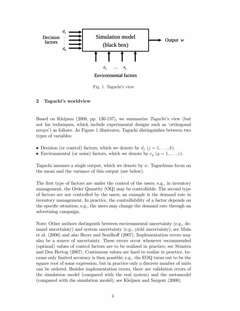
Fig. 1. Taguchi�s view
2 Taguchi�s worldview
Based on Kleijnen (2008, pp. 130-137), we summarize Taguchi�s view (butnot his techniques, which include experimental designs such as �orthogonalarrays�) as follows. As Figure 1 illustrates, Taguchi distinguishes between twotypes of variables:
� Decision (or control) factors, which we denote by dj (j = 1; : : : ; k).� Environmental (or noise) factors, which we denote by eg (g = 1; : : : ; c).
Taguchi assumes a single output, which we denote by w. Taguchians focus onthe mean and the variance of this output (see below).
The �rst type of factors are under the control of the users; e.g., in inventorymanagement, the Order Quantity (OQ) may be controllable. The second typeof factors are not controlled by the users; an example is the demand rate ininventory management. In practice, the controllability of a factor depends onthe speci�c situation; e.g., the users may change the demand rate through anadvertising campaign.
Note: Other authors distinguish between environmental uncertainty (e.g., de-mand uncertainty) and system uncertainty (e.g., yield uncertainty); see Mulaet al. (2006) and also Beyer and Sendho¤ (2007). Implementation errors mayalso be a source of uncertainty. These errors occur whenever recommended(optimal) values of control factors are to be realized in practice; see Stinstraand Den Hertog (2007). Continuous values are hard to realize in practice, be-cause only limited accuracy is then possible; e.g., the EOQ turns out to be thesquare root of some expression, but in practice only a discrete number of unitscan be ordered. Besides implementation errors, there are validation errors ofthe simulation model (compared with the real system) and the metamodel(compared with the simulation model); see Kleijnen and Sargent (2000).
4
As we mentioned above, we do not use Taguchi�s statistical methods. Our mainreason is that simulation experiments enable the exploration of many more fac-tors, factor levels, and combinations of factor levels than real-life (physical)experiments do. Moreover, we do not use Taguchi�s scalar output (such asthe signal-to-noise or mean-to-variance ratio); instead we allow each outputto have a statistical distribution (or density function), which we characterizethrough its mean and standard deviation; also see Beyer and Sendho¤ (2007),Lee and Nelder (2003), and Myers and Montgomery (1995, p. 491). So we feelthat a Taguchian loss function (see, e.g., Park et al. (2006)) is too restric-tive. We solve the resulting bi-objective problem through the Pareto-optimale¢ ciency frontier� brie�y called the Pareto frontier.
Note: The relevant problem formulation depends on the risk attitude of theusers (they might be risk-seeking optimists), which may vary with the appli-cation. We conjecture that our heuristic also applies to alternative problemformulations, but in this article we do not investigate these alternatives. Manyreferences on supply-chain risk-management are given in Wu et al. (2008), whofocus on the mean-variance trade-o¤ in the newsvendor�s inventory problem.The mean-variance trade-o¤ for simulation models is also examined by Apley,Liu, and Chen (2006) and Chen, Jin, and Sudjianto (2006).
3 RSM and robust optimization
To design and analyze our simulation experiments; we use RSM followingMyers and Montgomery (1995). RSM extends Taguchi�s simpler statisticaltechniques. The simplest RSM metamodel is a polynomial of a degree as lowas possible:
� Because we wish to estimate the optimal combination(s) of the decisionfactors dj (j = 1; : : : ; k), we �t a second-order polynomial for these factors.
� Moreover, we wish to model possible e¤ects of the environmental factors eg(g = 1; : : : ; c); we �t a �rst-order polynomial for these factors.
� Finally, we wish to estimate interactions between the two types of factors,so we �t �control-by-noise�two-factor interactions. (Interaction between djand eg implies nonparallel response surfaces for dj� given di¤erent valuesfor eg.)
5
Altogether we �t the following metamodel proposed by Myers and Mont-gomery (1995, p. 218, 492):
y = �0 +kXj=1
�jdj +kXj=1
kXj0�j
�j;j0djdj0 +cXg=1
jej +kXj=1
cXg=1
�j;gdjeg + �
= �0 + �0d+ d0Bd+ 0e+ d0�e+ �;
(1)
where y denotes the regression predictor of the simulation output w, � denotesthe residual with E(�) = 0 if this metamodel has no lack of �t (this zero meanshould be tested; see cross-validation below) and constant variance �2� (anunrealistic assumption in simulation experimentation), and the bold symbolsare the vectors and matrices that are de�ned in the obvious way (e.g., � =(�1; : : : ; �k)
0 and B denotes the k � k symmetric matrix with main-diagonalelements �j;j and o¤-diagonal elements �j;j0=2).
It is convenient and traditional in Design Of Experiments (DOE) to usecoded� also called standardized or scaled� factor values. Let the experimentconsist of n factor combinations of the �original� factors zj (zj correspondswith dj or eg in (1)); furthermore, let lj denote the lowest value of zj in theexperiment, and uj the highest (�upper�) value. Then the coded variable xjuse the linear transformation
xj = aj + bjzj with aj =lj + ujlj � uj
and bj =2
uj � lj. (2)
The term (uj � lj) is the range of input j. If z is a random variable (like e),then this coding implies var(x) = b2var(e). The numerical accuracy of theestimates may be a¤ected by coding; we focus on the estimated e¤ects of thecoded variables. Coding is further discussed by Kleijnen (2008, p. 29).
Assuming a model like (1), Myers and Montgomery (1995, p. 493-494) derivethe mean and the variance of y (the regression predictor of the simulationoutput w), after averaging over the noise factors� and assuming that the en-vironmental variables e satisfy
E(e) = 0 and cov(e) = �2eI. (3)
Obviously, assuming zero means and constant variances is unrealistic, so weshall replace (3) by (11). Given (3), they derive
E(y) = �0 + �0d+ d0Bd (4)
andvar(y) = �2e(
0 + d0�)( +�0d)+�2� = �2el0l+�2� ; (5)
where l = ( +�0d)= (@y=@e1; : : : ; @y=@ec)0; i.e., l is the gradient with respectto the environmental factors� which follows directly from (1). So, the larger
6
the gradient�s elements are, the larger the variance of the predicted simulationoutput is� which stands to reason. Furthermore, if� = 0 (no control-by-noiseinteractions), then var(y) cannot be controlled through the control variablesd.
Equation (5) implies that the predicted simulation output y has heterogeneousvariances� even if �2e and �
2� were constants� because changing the control fac-
tors d changes var(y). Whereas Myers and Montgomery (1995, p. ...) presentexamples with �2e = �2�=2, Kleijnen (2008, p. 136) gives a supply-chain sim-ulation with �2e = 10�2� . Most important is the gradient l, because it showsthe key role played by the control-by-noise interactions; i.e., to reduce thepredicted output�s variance var(y)(or �2y) the analysts should take advantageof the interactions�; they cannot control the main e¤ects of the noise factors( ) and the variances of the noise factors and the residuals (�2e and �
2�). For
example, if a particular decision factor (say, d1) has no e¤ects on the meanoutput (so �1 = �1;1 = �1;2 = : : : = �1;k = 0) but has important interactionswith the noise factors (e.g., �1;2 >> 0), then this interaction can be utilized todecrease the output variance (e.g., decrease �2y by decreasing d1). If there aremultiple decision factors, then the following solution method may be tried:
(1) select the values of some decision factors such that l = 0, so var(y) in (5)is minimized;
(2) select the remaining decision factors such that the predicted mean outputE(y) in (4) gets the desired value.
Myers and Montgomery (1995, p. 495) also discuss constrained optimization,which minimizes (e.g.) the variance (5) subject to a constraint on the mean(4). Often those authors simply superimpose contour plots for the mean andvariance, to select an appropriate compromise or �robust�solution. We shalluse Mathematical Programming, which is more general and �exible.
To estimate the unknown (regression) parameters in (1)� which also gives theparameters in the mean and variance equations (4) and (5)� we reformulate(1) as the following linear regression model :
y = � 0x+ � (6)
with � = (�0;�;b; ; �)0 where b denotes the vector with the k � (k � 1)=2
interactions between the decision factors plus their k purely quadratic e¤ects,and � denotes the k�c control-by-noise interactions; x is de�ned in the obviousway (e.g., the element corresponding with the interaction e¤ect �1;2 is d1d2).
If we use the Least Squares (LS) criterion, then (6) gives the Ordinary LS(OLS) estimator b� = (X0X)�1X0w; (7)
7
where X is the n � q matrix of explanatory variables with n denoting thenumber of scenarios (combinations of decision and environmental factors) de-termined by DOE that are actually simulated, and q denotes the number ofparameters collected in �; this X is assumed not to be collinear (otherwise,(X0X)�1 would not exist). So a necessary but not su¢ cient condition for X isn > q. The vector w consists of the n simulation outputs.
The covariance matrix of the OLS estimator, cov(b�), is needed to test theimportance of the estimated e¤ects. If �2w were constant, then (7) would imply
cov(b�) =(X0X)�1�2w: (8)
Note: We might use this equation to �nd a design that is �D-optimal�; i.e., adesign that minimizes the determinant of cov(b�); see Chung, Goldfarb, andMontgomery (2007).
In order to apply classic OLS results, we assume that �2w is constant, the out-puts for di¤erent scenarios are independent, and the environmental factors are�xed (Myers and Montgomery (1995, p. 490) do not make these assumptionsexplicit; in our EOQ application we can derive the true Pareto optimum, sowe can verify how sensitive our analysis is to these assumptions). Then theclassic estimator of �2� is the Mean Squared Residuals (MSR)
MSR =(by �w)0(by �w)
n� q (9)
where by = b� 0x; also see Kleijnen (2000, p. 23). Note that �2e is known becausethe environmental factors are sampled from a known distribution. So var(y)can be estimated through substitution of the estimator MSR for �2� into (5).
Moreover, we assume that the simulation outputs w are normally distributed;i.e., we assume that the environmental variables e and the noise � in (1)are normally distributed. The OLS estimator b� in (7) is then also normallydistributed. Consequently, the individual estimated regression parameters c�jmay be tested through the following t statistic with n� q degrees of freedom:
tn�q =c�j � �js(c�j) with j = 1; : : : ; q (10)
where s(c�j) is the square root of the jth element on the main diagonal ofthe covariance matrix for b� given in (8) with �2w estimated through the MSRde�ned in (9). It is well-known that the t statistic is not very sensitive tononnormality; see Kleijnen (1987).
8
Myers and Montgomery (1995, p. 488) keep only the signi�cant e¤ects intheir response model. We agree that when estimating the robust optimum,we should use the reduced metamodel, which eliminates all non-signi�cante¤ects in the full model� except for those non-signi�cant e¤ects that involvefactors that have signi�cant higher-order e¤ects; e.g., if the estimated maine¤ect c�1 is not signi�cant but the estimated quadratic e¤ect d�1;1 is, thenc�1 is not set to zero. We point out that the (possibly non-signi�cant) OLSestimator is the Best Linear Unbiased Estimator (BLUE) so we must havegood reasons to replace it by zero (also see the �strong heredity�assumptionin Wu and Hamada (2000)). The reduced metamodel may imply a uniqueoptimum, whereas the full metamodel may suggest (say) a saddlepoint. To �ndthe unimportant e¤ects, Myers and Montgomery (1995, p. 487) use ANalysisOf VAriance (ANOVA). Note that t2n�q = F1;n�q; the F statistic is used inANOVA.
To construct con�dence intervals for the robust optimum Myers and Mont-gomery (1995, p. 498) assume normality, which results in an F statistic. Myersand Montgomery (1995, p. 504) notice that the analysis becomes complicatedwhen the noise factors do not have constant variances. We shall therefore useparametric bootstrapping for RSM applied to the EOQ examples; by de�ni-tion, parametric bootstrapping assumes that the distribution of the relevantrandom variable is known (in the EOQ examples, we assume that the distribu-tion is Gaussian). In general bootstrapping is a simple numerical/computerizedmethod for obtaining the Estimated Density Function (EDF) of a� possiblycomplicated� statistic for a� possibly non-Gaussian� parent distribution. Ex-amples are the well-known Student statistic for a non-Gaussian parent distri-bution, and the statistic that is formed by the solution of a Nonlinear Pro-gramming problem with Gaussian inputs (as is the case for our study). Moredetails are given by Efron and Tibshirani (1993), Kleijnen (2008, p. 86), andKleijnen, Van Beers, and Van Nieuwenhuyse (2008).
Note: Myers and Montgomery (1995, p. 508) discuss the use of transformationsof the dependent variable, before performing the regression analysis; also seeKleijnen (2008, p. 98).
Finally, we replace Myers and Montgomery�s assumption formulated in (3) by
E(e) = �e and cov(e) = e: (11)
Then (4) becomes
E(y) = �0 + �0d+ d0Bd+ 0�e + d
0��e (12)
and (5) becomes
var(y) = ( 0 + d0�)e( +�0d)+�2� = l
0el+�2� : (13)
9
To estimate the left-hand side of (12), we simply plug in the estimators for �0,�, B, , and � in the right-hand side (the factors d and �e are known). Toestimate the left-hand side of (13), we again use plug-in estimators� now for , �, and �2� (the factor e is known); see Myers and Montgomery (1995, p.495). However, we point out that (13) has products of unknown parameters,
so it implies a nonlinear estimator c�2y (we are also interested in c�y = qc�2y, anonlinear transformation of c�2y) so this plug-in estimator is certainly biased;this bias we ignore when estimating the Pareto frontier that balances by and c�y.To study the variability of this estimated Pareto frontier (caused by the noisefollowing from estimating the regression parameters), we use bootstrapping.
The estimation of the mean and variance of the simulation output through (12)and (13) raises the following crucial question (also raised by Myers and Mont-gomery (1995, pp. 41-54), but assuming a constant output variance): Is theunderlying RSM model (1) an adequate approximation? The linear regressionliterature presents several methods for answering this question; see Kleijnen(2008, p. 54). We focus on a method that is also applied outside linear regres-sion (e.g. in Kriging), namely cross-validation. There are several variationson cross-validation (see Iooss, Ribatet, and Marrel (2007) and Meckesheimeret al. (2001)), but the most popular variant is leave-one-out cross-validation.Following Kleijnen (2008, p. 57), we de�ne this cross-validation as follows.
(1) Delete I/O combination i from the complete set of n combinations, toobtain the remaining I/O data set� denoted by (X�i;w�i). Assume thatthis step results in an (n� 1)� q noncollinear matrix X�i (i = 1; : : : ; n);a necessary condition is n > q. Obviously, w�i denotes the (n � 1)-dimensional vector with the remaining (n� 1) simulation outputs.
(2) Recompute the OLS estimator of the regression parameters in (7):
d��i = (X0�iX�i)
�1X0�iw�i. (14)
(3) Use d��i (recomputed regression parameters) to compute dy�i, which de-notes the regression predictor of the simulation output generated by xi(which corresponds with the simulation input of the combination deletedin step 1): dy�i = x0id��i. (15)
(4) Repeat the preceding three steps, until all n combinations have beenprocessed. This results in n predictions dy�i (i = 1; : : : ; n).
(5) Use a scatterplot with the n pairs (wi;dy�i) to judge whether the meta-model is valid.
(6) Because the scaling of this scatterplot may give the wrong impression,we also evaluate the relative prediction errors dy(�i)=wi.
(7) A valid regression model also implies that the estimated regression coe¢ -cients do not change much when deleting an I/O combination; i.e., there
10
is not much change in d��i with (i = 0; 1; : : : ; n) where d��0 denotes theestimator when zero combinations are deleted, so d��0 = c�.
Our �nal goal in robust optimization is to minimize the estimated mean by�which assumes that (12) is an adequate approximation� while keeping the es-timated standard deviation c�y� which assumes that (13) is adequate� belowa given Threshold (say) T . We solve this constrained minimization problemthrough Matlab�s �fmincon�, which gives the values of the �estimated robustdecision variables�(say) dd+ and its corresponding mean by and standard de-viation c�y. Next, we vary the threshold value T (say) 100 times, which maygive a di¤erent solutiondd+ with its corresponding by and c�y. Then, we collectthe 100 pairs (by; c�y) to estimate the Pareto frontier. Finally, we estimate thevariability of this frontier curve through bootstrapping of the estimated re-gression estimates that gave by and c�y. We shall illustrate our methodology inthe next section.
4 EOQ inventory simulation
We apply our methodology to the simulation optimization of the classic EOQinventory model, which is often used in practical supply chain management.First, we de�ne the EOQ model, including symbols and assumptions; also seePentico, Drake, and Toews (2008) and Teng (2008). Following Zipkin (2000,pp. 30-39), we use the following assumptions:
(1) The demand is known and constant, say a units per time unit.(2) The order quantity is Q units.(3) No shortages are allowed.(4) Delivery lead time is zero; i.e., the order arrives into inventory as soon as
the order is placed.(5) Review is continuous; i.e. an order is placed as soon as the inventory level
drops to the reorder point, which is set to zero because of assumptions 1and 4.
(6) Total costs has the following components:� setup cost per order, K� cost per unit purchased or produced, c� holding cost per inventory unit per time unit, h.
De�ning a �cycle�as the period between two consecutive replenishments, thecycle length is obviously Q=a. The cost per time unit is simply the total costover one cycle divided by the cycle length. The goal is to minimize the costsper time unit (say) C, over an in�nite time horizon.
11
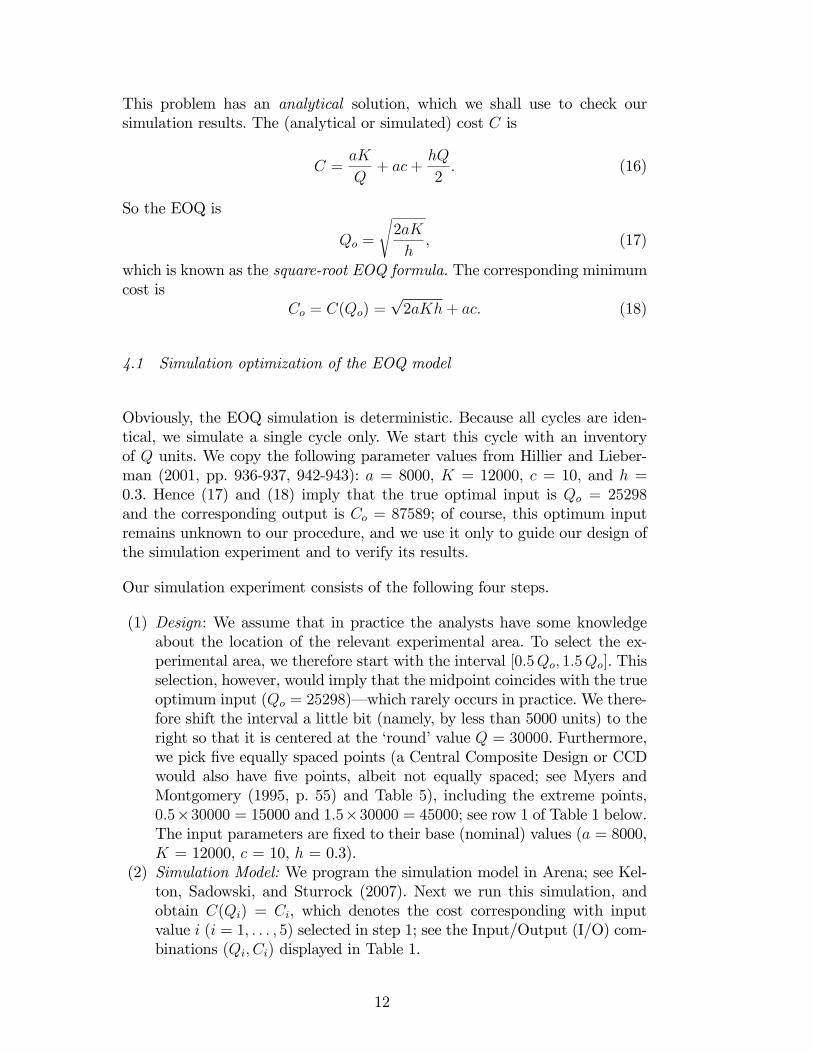
This problem has an analytical solution, which we shall use to check oursimulation results. The (analytical or simulated) cost C is
C =aK
Q+ ac+
hQ
2: (16)
So the EOQ is
Qo =
s2aK
h; (17)
which is known as the square-root EOQ formula. The corresponding minimumcost is
Co = C(Qo) =p2aKh+ ac: (18)
4.1 Simulation optimization of the EOQ model
Obviously, the EOQ simulation is deterministic. Because all cycles are iden-tical, we simulate a single cycle only. We start this cycle with an inventoryof Q units. We copy the following parameter values from Hillier and Lieber-man (2001, pp. 936-937, 942-943): a = 8000, K = 12000, c = 10, and h =0.3. Hence (17) and (18) imply that the true optimal input is Qo = 25298and the corresponding output is Co = 87589; of course, this optimum inputremains unknown to our procedure, and we use it only to guide our design ofthe simulation experiment and to verify its results.
Our simulation experiment consists of the following four steps.
(1) Design: We assume that in practice the analysts have some knowledgeabout the location of the relevant experimental area. To select the ex-perimental area, we therefore start with the interval [0:5Qo; 1:5Qo]. Thisselection, however, would imply that the midpoint coincides with the trueoptimum input (Qo = 25298)� which rarely occurs in practice. We there-fore shift the interval a little bit (namely, by less than 5000 units) to theright so that it is centered at the �round�value Q = 30000. Furthermore,we pick �ve equally spaced points (a Central Composite Design or CCDwould also have �ve points, albeit not equally spaced; see Myers andMontgomery (1995, p. 55) and Table 5), including the extreme points,0:5�30000 = 15000 and 1:5�30000 = 45000; see row 1 of Table 1 below.The input parameters are �xed to their base (nominal) values (a = 8000,K = 12000, c = 10, h = 0.3).
(2) Simulation Model: We program the simulation model in Arena; see Kel-ton, Sadowski, and Sturrock (2007). Next we run this simulation, andobtain C(Qi) = Ci, which denotes the cost corresponding with inputvalue i (i = 1; : : : ; 5) selected in step 1; see the Input/Output (I/O) com-binations (Qi; Ci) displayed in Table 1.
12
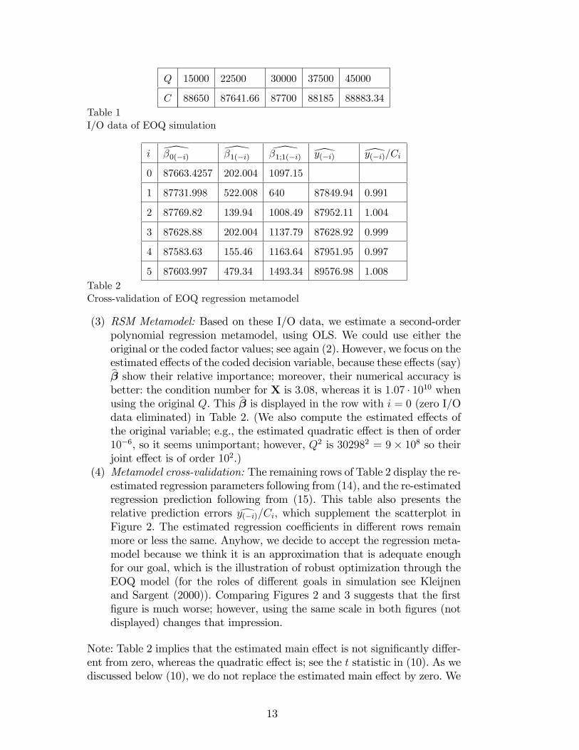
Q 15000 22500 30000 37500 45000
C 88650 87641.66 87700 88185 88883.34Table 1I/O data of EOQ simulation
i \�0(�i) \�1(�i) \�1;1(�i) [y(�i) [y(�i)=Ci
0 87663.4257 202.004 1097.15
1 87731.998 522.008 640 87849.94 0.991
2 87769.82 139.94 1008.49 87952.11 1.004
3 87628.88 202.004 1137.79 87628.92 0.999
4 87583.63 155.46 1163.64 87951.95 0.997
5 87603.997 479.34 1493.34 89576.98 1.008Table 2Cross-validation of EOQ regression metamodel
(3) RSM Metamodel: Based on these I/O data, we estimate a second-orderpolynomial regression metamodel, using OLS. We could use either theoriginal or the coded factor values; see again (2). However, we focus on theestimated e¤ects of the coded decision variable, because these e¤ects (say)b� show their relative importance; moreover, their numerical accuracy isbetter: the condition number for X is 3:08, whereas it is 1:07 � 1010 whenusing the original Q. This b� is displayed in the row with i = 0 (zero I/Odata eliminated) in Table 2. (We also compute the estimated e¤ects ofthe original variable; e.g., the estimated quadratic e¤ect is then of order10�6, so it seems unimportant; however, Q2 is 302982 = 9� 108 so theirjoint e¤ect is of order 102.)
(4) Metamodel cross-validation: The remaining rows of Table 2 display the re-estimated regression parameters following from (14), and the re-estimatedregression prediction following from (15). This table also presents therelative prediction errors dy(�i)=Ci, which supplement the scatterplot inFigure 2. The estimated regression coe¢ cients in di¤erent rows remainmore or less the same. Anyhow, we decide to accept the regression meta-model because we think it is an approximation that is adequate enoughfor our goal, which is the illustration of robust optimization through theEOQ model (for the roles of di¤erent goals in simulation see Kleijnenand Sargent (2000)). Comparing Figures 2 and 3 suggests that the �rst�gure is much worse; however, using the same scale in both �gures (notdisplayed) changes that impression.
Note: Table 2 implies that the estimated main e¤ect is not signi�cantly di¤er-ent from zero, whereas the quadratic e¤ect is; see the t statistic in (10). As wediscussed below (10), we do not replace the estimated main e¤ect by zero. We
13
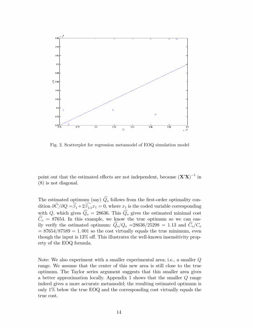
Fig. 2. Scatterplot for regression metamodel of EOQ simulation model
point out that the estimated e¤ects are not independent, because (X0X)�1 in(8) is not diagonal.
The estimated optimum (say) cQo follows from the �rst-order optimality con-dition @ bC=@Q =c�1+2d�1;1x1 = 0, where x1 is the coded variable correspondingwith Q, which gives cQo = 28636. This cQo gives the estimated minimal costcCo = 87654. In this example, we know the true optimum so we can eas-ily verify the estimated optimum: cQo=Qo =28636=25298 = 1:13 and cCo=Co= 87654=87589 = 1: 001 so the cost virtually equals the true minimum, eventhough the input is 13% o¤. This illustrates the well-known insensitivity prop-erty of the EOQ formula.
Note: We also experiment with a smaller experimental area; i.e., a smaller Qrange. We assume that the center of this new area is still close to the trueoptimum. The Taylor series argument suggests that this smaller area givesa better approximation locally. Appendix 1 shows that the smaller Q rangeindeed gives a more accurate metamodel; the resulting estimated optimum isonly 1% below the true EOQ and the corresponding cost virtually equals thetrue cost.
14
4.2 Robust optimization of EOQ model
Next, we drop Assumption 1 in Section 4, which stated that the demand is aknown constant a. We still assume that the demand per time unit is constant,but this constant is unknown. Many references on inventory management withuncertain parameters are given by Borgonovo and Peccati (2007).
Note: Yu (1997) also assumes an uncertain demand rate, but uses other cri-teria than we do: he either minimizes the maximum costs or minimizes themaximum percentage deviation from the optimal cost. Moreover he does notassume a probability function for the various scenarios (demand rate values),but uses �a discrete scenario set�. Altogether, his approach resembles that ofBen-Tal et al., which we discussed in the Introduction.
Note: The assumption of uncertain constants is often made in deterministicsimulation of physical systems; e.g., a nuclear waste-disposal simulation mayassume that the permeability of a speci�c area is constant but unknown; seeKleijnen and Helton (1999). An economic example is the exchange rate be-tween the US dollar and the euro exactly one year from today: that rate is aconstant but unknown.
We may collect historical data to infer the probability of the true value of theparameter a. If there is no such data, then we may ask experts for their opinionon the true value of the parameter. This knowledge elicitation results in aninput distribution (say) F (a). In practice, several distribution types are used,such as normal, lognormal, and uniform; see Kleijnen and Helton (1999). Inour experiments we assume� without loss of generality� that a has a Normal(Gaussian) distribution with mean �a and standard deviation �a:
a � N(�a; �a): (19)
More speci�cally, we assume that �a denotes the �base�or �nominal�value thatwas used in the simulation optimization of the EOQ model in Section 4.1, and�a quanti�es the uncertainty about the true input parameter. We experimentwith a �low�and �high�uncertainty: �a = 0:10�a and �a= 0:50�a. Becausethese standard deviations can give a negative value for a, we resample untilwe get non-negative values only; i.e., we adjust the normal distribution in (19)slightly. However, we ignore this adjustment in our further analysis.
Following Myers and Montgomery (1995, pp. 463-534), we select �a few�values(levels) for the environmental factors. Those authors use only two values perenvironmental factor (which su¢ ces to estimate its main e¤ect and its inter-actions with the decision factors). We, however, use Latin Hypercube Sampling(LHS) to select �a few�values for the environmental factors (because LHS ispopular in risk and uncertainty analysis; see Kleijnen 2008), which runs as
15
Q n a 4530,34 5478,85 7687,37 9329,26 11559,02
15000 51177,72 61421,54 85273,65 103006 127087,4
22500 51094,63 61085,52 84348,68 101643,2 125130
30000 51615,59 61480 84448,7 101524,3 124713,8
37500 52378,16 62166,7 84958,71 101902,9 124914,1
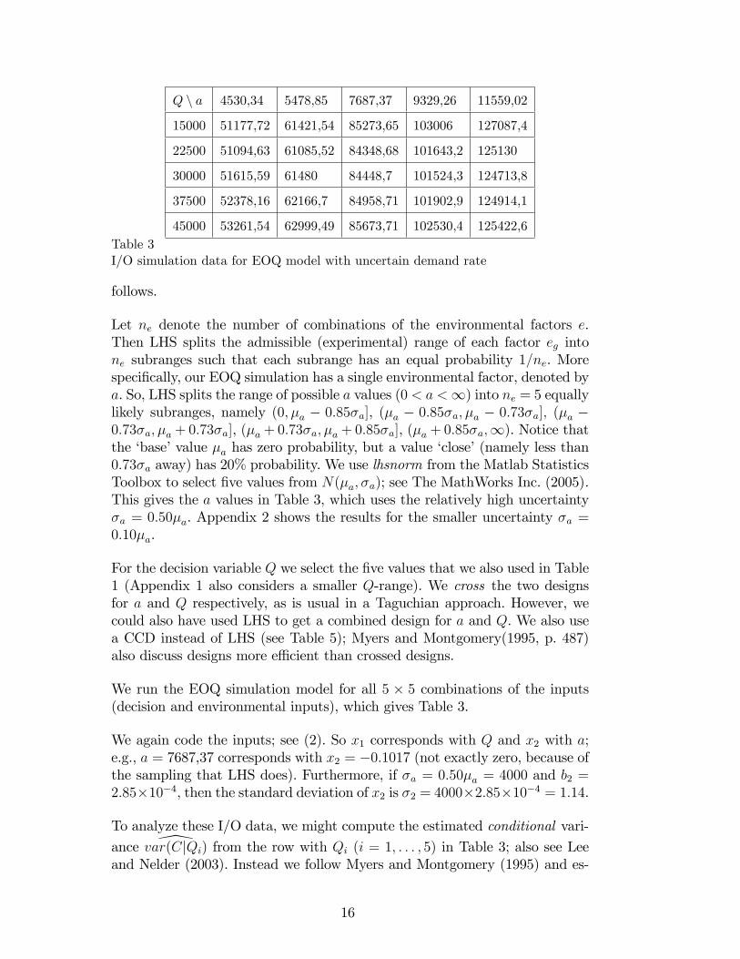
45000 53261,54 62999,49 85673,71 102530,4 125422,6Table 3I/O simulation data for EOQ model with uncertain demand rate
follows.
Let ne denote the number of combinations of the environmental factors e.Then LHS splits the admissible (experimental) range of each factor eg intone subranges such that each subrange has an equal probability 1=ne. Morespeci�cally, our EOQ simulation has a single environmental factor, denoted bya. So, LHS splits the range of possible a values (0 < a <1) into ne = 5 equallylikely subranges, namely (0; �a � 0:85�a], (�a � 0:85�a; �a � 0:73�a]; (�a �0:73�a; �a + 0:73�a], (�a + 0:73�a; �a + 0:85�a], (�a + 0:85�a;1). Notice thatthe �base�value �a has zero probability, but a value �close�(namely less than0:73�a away) has 20% probability. We use lhsnorm from the Matlab StatisticsToolbox to select �ve values from N(�a; �a); see The MathWorks Inc. (2005).This gives the a values in Table 3, which uses the relatively high uncertainty�a = 0:50�a. Appendix 2 shows the results for the smaller uncertainty �a =0:10�a.
For the decision variable Q we select the �ve values that we also used in Table1 (Appendix 1 also considers a smaller Q-range). We cross the two designsfor a and Q respectively, as is usual in a Taguchian approach. However, wecould also have used LHS to get a combined design for a and Q. We also usea CCD instead of LHS (see Table 5); Myers and Montgomery(1995, p. 487)also discuss designs more e¢ cient than crossed designs.
We run the EOQ simulation model for all 5 � 5 combinations of the inputs(decision and environmental inputs), which gives Table 3.
We again code the inputs; see (2). So x1 corresponds with Q and x2 with a;e.g., a = 7687,37 corresponds with x2 = �0:1017 (not exactly zero, because ofthe sampling that LHS does). Furthermore, if �a = 0:50�a = 4000 and b2 =2:85�10�4, then the standard deviation of x2 is �2 = 4000�2:85�10�4 = 1:14.
To analyze these I/O data, we might compute the estimated conditional vari-
ance \var(CjQi) from the row with Qi (i = 1; : : : ; 5) in Table 3; also see Leeand Nelder (2003). Instead we follow Myers and Montgomery (1995) and es-
16

Fig. 3. Scatterplot of regression metamodel for RO of EOQ
timate the variance using all the elements in this table; also see (13). Thelatter approach gives a better estimator, provided the RSM metamodel (1) iscorrect.
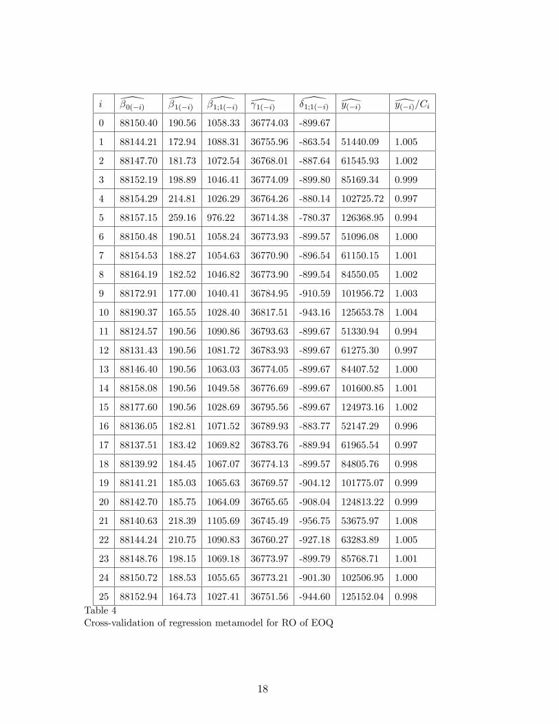
To compute the OLS estimates, we must re-arrange the 5 � 5 elements ofTable 3 into the n � q X-matrix of (7) where now n = 25 and q = 5; w nowbecomes a vector with the 25 simulation outputs C. This gives the estimatedintercept c�0, the estimated �rst-order e¤ect c�1 and second-order e¤ect d�1;1 ofQ, the estimated �rst-order e¤ect c 1 of a, and the interaction d�1;1, which aredisplayed in the row denoted by 0 (zero rows eliminated) in Table 4. The restof this table displays the cross-validation results (analogous to Table 2). Thistable gives the scatterplot in Figure 3. This table and this �gure suggest thatthis metamodel is adequate for robust optimization through RSM.
Note: Appendices 1 and 2 give results for a smaller range of the decisionvariable Q and the environmental variable a. These results show even better�t.
Note: To check the negative sign of d�1;1 (interaction between Q and a), we usethe analytical solution (16) to derive @2C=@Q@a = �K=Q2, which is indeednegative.
Using a RSM metamodel like the one in the �rst row of Table 4, Myers andMontgomery (1995, p. 501) derive contour plots for the mean and variance. Be-
17
i \�0(�i) \�1(�i) \�1;1(�i) \ 1(�i) \�1;1(�i) [y(�i) [y(�i)=Ci
0 88150.40 190.56 1058.33 36774.03 -899.67
1 88144.21 172.94 1088.31 36755.96 -863.54 51440.09 1.005
2 88147.70 181.73 1072.54 36768.01 -887.64 61545.93 1.002
3 88152.19 198.89 1046.41 36774.09 -899.80 85169.34 0.999
4 88154.29 214.81 1026.29 36764.26 -880.14 102725.72 0.997
5 88157.15 259.16 976.22 36714.38 -780.37 126368.95 0.994
6 88150.48 190.51 1058.24 36773.93 -899.57 51096.08 1.000
7 88154.53 188.27 1054.63 36770.90 -896.54 61150.15 1.001
8 88164.19 182.52 1046.82 36773.90 -899.54 84550.05 1.002
9 88172.91 177.00 1040.41 36784.95 -910.59 101956.72 1.003
10 88190.37 165.55 1028.40 36817.51 -943.16 125653.78 1.004
11 88124.57 190.56 1090.86 36793.63 -899.67 51330.94 0.994
12 88131.43 190.56 1081.72 36783.93 -899.67 61275.30 0.997
13 88146.40 190.56 1063.03 36774.05 -899.67 84407.52 1.000
14 88158.08 190.56 1049.58 36776.69 -899.67 101600.85 1.001
15 88177.60 190.56 1028.69 36795.56 -899.67 124973.16 1.002
16 88136.05 182.81 1071.52 36789.93 -883.77 52147.29 0.996
17 88137.51 183.42 1069.82 36783.76 -889.94 61965.54 0.997
18 88139.92 184.45 1067.07 36774.13 -899.57 84805.76 0.998
19 88141.21 185.03 1065.63 36769.57 -904.12 101775.07 0.999
20 88142.70 185.75 1064.09 36765.65 -908.04 124813.22 0.999
21 88140.63 218.39 1105.69 36745.49 -956.75 53675.97 1.008
22 88144.24 210.75 1090.83 36760.27 -927.18 63283.89 1.005
23 88148.76 198.15 1069.18 36773.97 -899.79 85768.71 1.001
24 88150.72 188.53 1055.65 36773.21 -901.30 102506.95 1.000
25 88152.94 164.73 1027.41 36751.56 -944.60 125152.04 0.998Table 4Cross-validation of regression metamodel for RO of EOQ
18
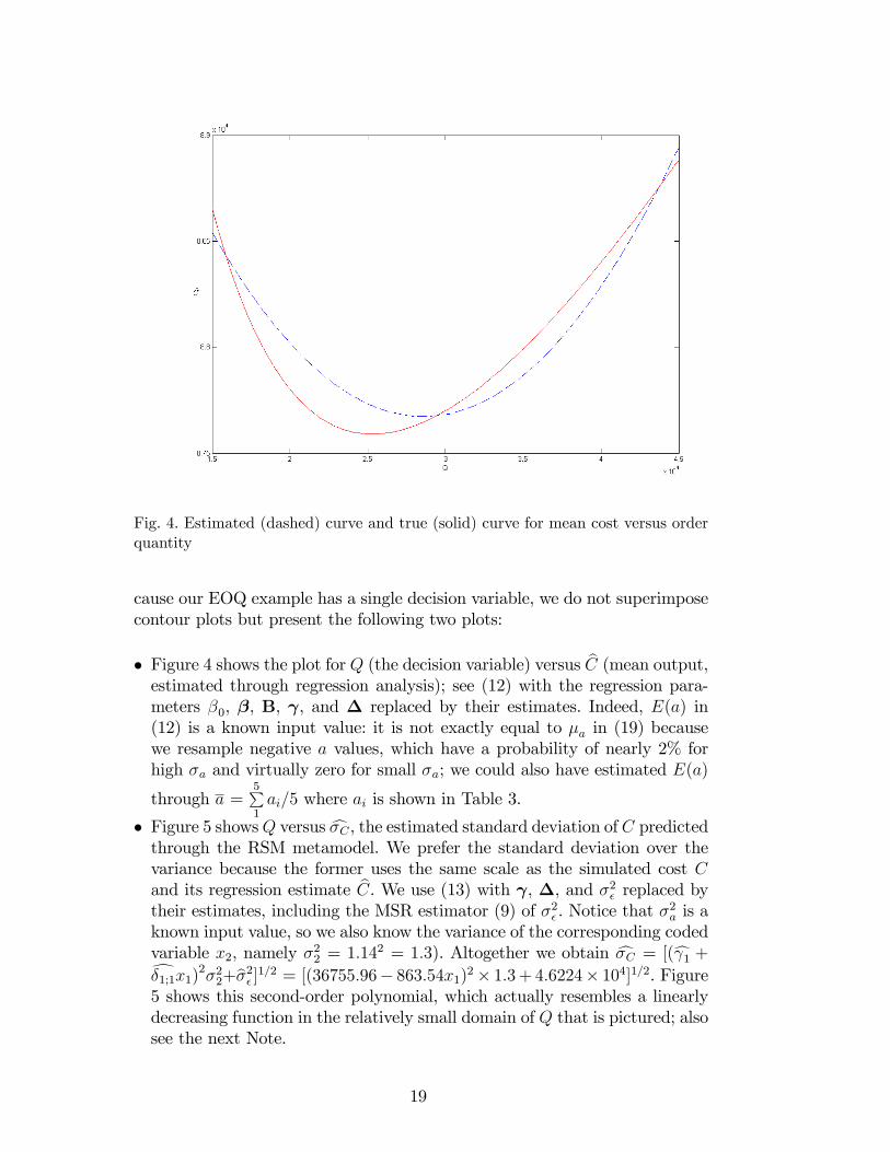
Fig. 4. Estimated (dashed) curve and true (solid) curve for mean cost versus orderquantity
cause our EOQ example has a single decision variable, we do not superimposecontour plots but present the following two plots:
� Figure 4 shows the plot for Q (the decision variable) versus bC (mean output,estimated through regression analysis); see (12) with the regression para-meters �0, �, B, , and � replaced by their estimates. Indeed, E(a) in(12) is a known input value: it is not exactly equal to �a in (19) becausewe resample negative a values, which have a probability of nearly 2% forhigh �a and virtually zero for small �a; we could also have estimated E(a)
through a =5P1ai=5 where ai is shown in Table 3.
� Figure 5 showsQ versus c�C , the estimated standard deviation of C predictedthrough the RSM metamodel. We prefer the standard deviation over thevariance because the former uses the same scale as the simulated cost Cand its regression estimate bC. We use (13) with , �, and �2� replaced bytheir estimates, including the MSR estimator (9) of �2� . Notice that �
2a is a
known input value, so we also know the variance of the corresponding codedvariable x2, namely �22 = 1:142 = 1:3). Altogether we obtain c�C = [(c 1 +d�1;1x1)2�22+b�2� ]1=2 = [(36755:96� 863:54x1)2� 1:3+ 4:6224� 104]1=2. Figure5 shows this second-order polynomial, which actually resembles a linearlydecreasing function in the relatively small domain of Q that is pictured; alsosee the next Note.
19
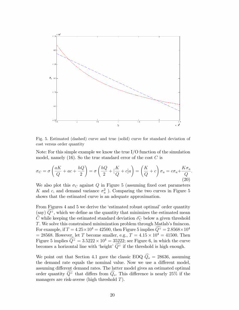
Fig. 5. Estimated (dashed) curve and true (solid) curve for standard deviation ofcost versus order quantity
Note: For this simple example we know the true I/O function of the simulationmodel, namely (16). So the true standard error of the cost C is
�C = �
aK
Q+ ac+
hQ
2
!= �
hQ
2+ [K
Q+ c]a
!=
K
Q+ c
!�a = c�a+
K�aQ:
(20)We also plot this �C against Q in Figure 5 (assuming �xed cost parametersK and c, and demand variance �2a ). Comparing the two curves in Figure 5shows that the estimated curve is an adequate approximation.
From Figures 4 and 5 we derive the �estimated robust optimal�order quantity(say) dQ+, which we de�ne as the quantity that minimizes the estimated meanbC while keeping the estimated standard deviation c�C below a given thresholdT . We solve this constrained minimization problem through Matlab�s fmincon.For example, if T = 4:25�104 = 42500, then Figure 5 impliesdQ+ = 2:8568�104= 28568. However, let T become smaller, e.g., T = 4:15� 104 = 41500. ThenFigure 5 implies dQ+ = 3:5222� 104 = 35222; see Figure 6, in which the curvebecomes a horizontal line with �height�dQ+ if the threshold is high enough.We point out that Section 4.1 gave the classic EOQ cQo = 28636, assumingthe demand rate equals the nominal value. Now we use a di¤erent model,assuming di¤erent demand rates. The latter model gives an estimated optimalorder quantity dQ+ that di¤ers from cQo. This di¤erence is nearly 25% if themanagers are risk-averse (high threshold T ).
20
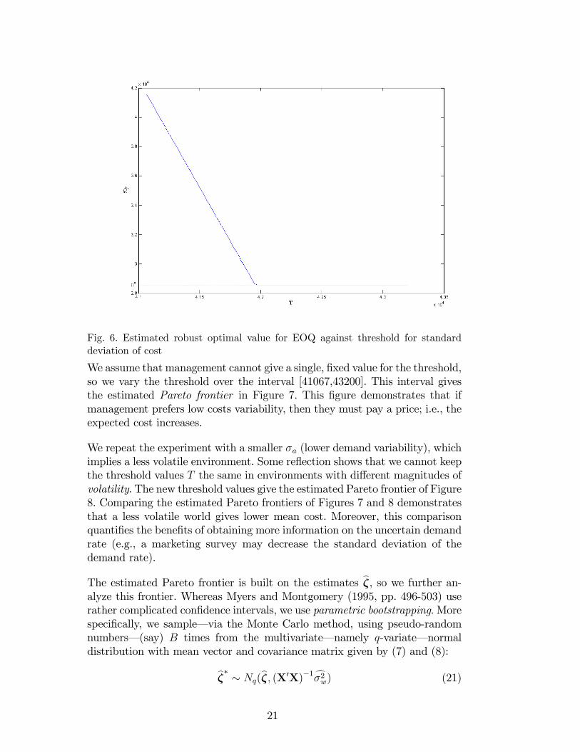
Fig. 6. Estimated robust optimal value for EOQ against threshold for standarddeviation of cost
We assume that management cannot give a single, �xed value for the threshold,so we vary the threshold over the interval [41067,43200]. This interval givesthe estimated Pareto frontier in Figure 7. This �gure demonstrates that ifmanagement prefers low costs variability, then they must pay a price; i.e., theexpected cost increases.
We repeat the experiment with a smaller �a (lower demand variability), whichimplies a less volatile environment. Some re�ection shows that we cannot keepthe threshold values T the same in environments with di¤erent magnitudes ofvolatility. The new threshold values give the estimated Pareto frontier of Figure8. Comparing the estimated Pareto frontiers of Figures 7 and 8 demonstratesthat a less volatile world gives lower mean cost. Moreover, this comparisonquanti�es the bene�ts of obtaining more information on the uncertain demandrate (e.g., a marketing survey may decrease the standard deviation of thedemand rate).
The estimated Pareto frontier is built on the estimates b�, so we further an-alyze this frontier. Whereas Myers and Montgomery (1995, pp. 496-503) userather complicated con�dence intervals, we use parametric bootstrapping. Morespeci�cally, we sample� via the Monte Carlo method, using pseudo-randomnumbers� (say) B times from the multivariate� namely q-variate� normaldistribution with mean vector and covariance matrix given by (7) and (8):
b�� � Nq(b�; (X0X)�1c�2w) (21)
21
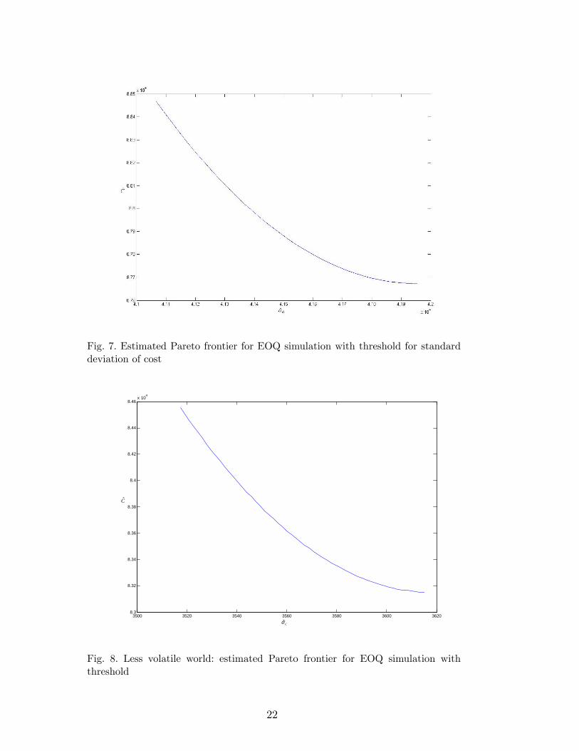
Fig. 7. Estimated Pareto frontier for EOQ simulation with threshold for standarddeviation of cost
3500 3520 3540 3560 3580 3600 36208.3
8.32
8.34
8.36
8.38
8.4
8.42
8.44
8.46x 10
4
s(C)
E(C
)
Cσ
C
3500 3520 3540 3560 3580 3600 36208.3
8.32
8.34
8.36
8.38
8.4
8.42
8.44
8.46x 10
4
s(C)
E(C
)
Cσ
C
Fig. 8. Less volatile world: estimated Pareto frontier for EOQ simulation withthreshold
22
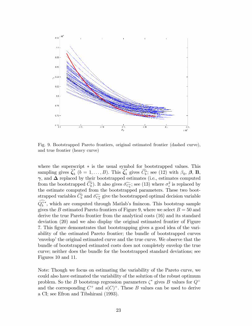
Fig. 9. Bootstrapped Pareto frontiers, original estimated frontier (dashed curve),and true frontier (heavy curve)
where the superscript � is the usual symbol for bootstrapped values. Thissampling gives b��b (b = 1; : : : ; B). This b��b gives cC�b ; see (12) with �0, �, B, , and � replaced by their bootstrapped estimates (i.e., estimates computedfrom the bootstrapped cC�b ). It also gives d�C�b ; see (13) where �2� is replaced bythe estimate computed from the bootstrapped parameters. These two boot-strapped variables cC�b and d�C�b give the bootstrapped optimal decision variabledQ+�b , which are computed through Matlab�s fmincon. This bootstrap samplegives the B estimated Pareto frontiers of Figure 9, where we select B = 50 andderive the true Pareto frontier from the analytical costs (16) and its standarddeviation (20) and we also display the original estimated frontier of Figure7. This �gure demonstrates that bootstrapping gives a good idea of the vari-ability of the estimated Pareto frontier; the bundle of bootstrapped curves�envelop�the original estimated curve and the true curve. We observe that thebundle of bootstrapped estimated costs does not completely envelop the truecurve; neither does the bundle for the bootstrapped standard deviations; seeFigures 10 and 11.
Note: Though we focus on estimating the variability of the Pareto curve, wecould also have estimated the variability of the solution of the robust optimumproblem. So the B bootstrap regression parameters �� gives B values for Q+
and the corresponding C+ and s(C)+. These B values can be used to derivea CI; see Efron and Tibshirani (1993).
23
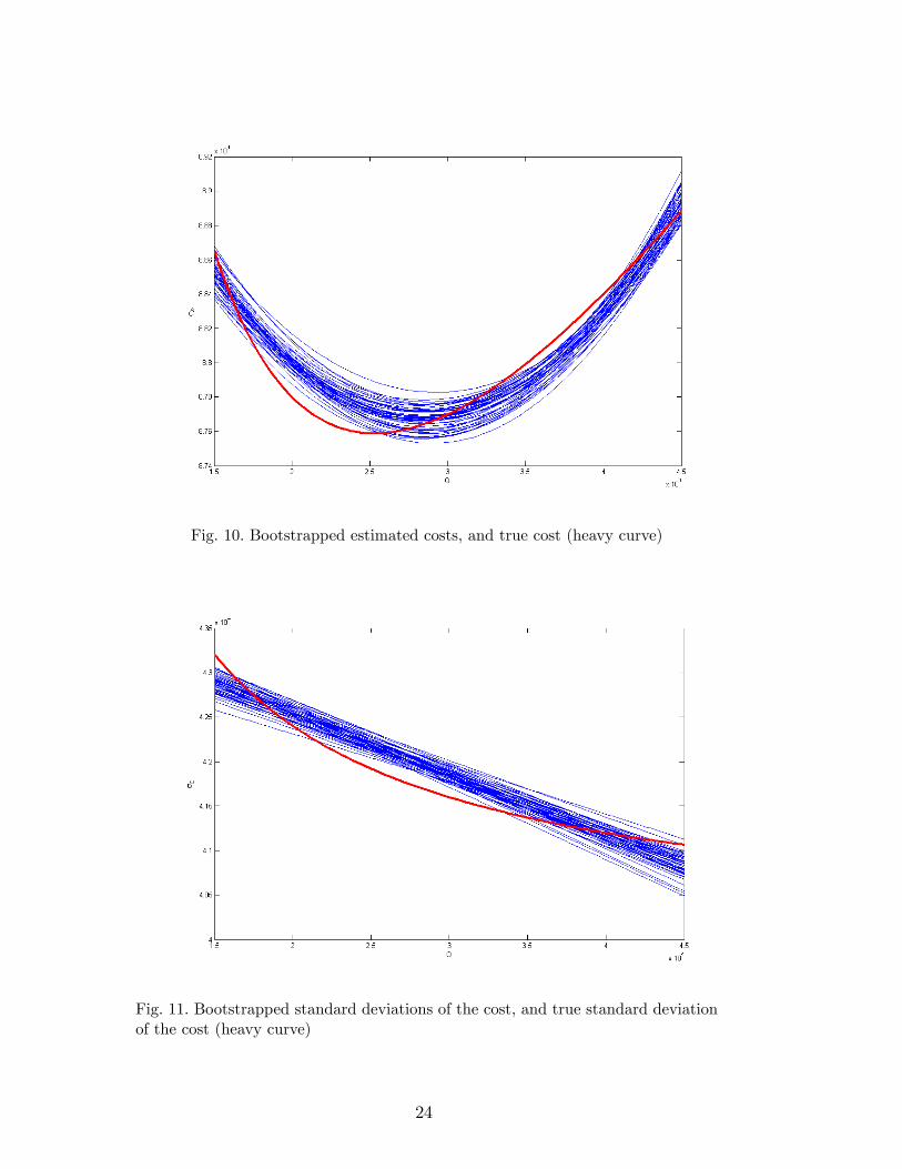
Fig. 10. Bootstrapped estimated costs, and true cost (heavy curve)
Fig. 11. Bootstrapped standard deviations of the cost, and true standard deviationof the cost (heavy curve)
24
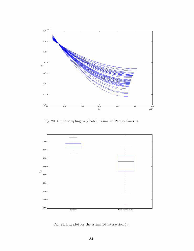
Note: Actually, we can validate our (fast) bootstrap procedure as follows OurEOQ simulation is the opposite of expensive simulation: some realistic simu-lations take hours or weeks for a single run, whereas bootstrapping this simu-lation�s results still takes only seconds. So we repeat our LHS sample (say) Ltimes; i.e., we sample the demand rate a from the normal distribution in (19)cut-o¤ at zero, while keeping the �ve Q values in Table 3 �xed. This sample ofL macroreplicates gives the regression estimate b�l with l = 1; : : : ; L. This b�lgives cCl (costs estimated through RSM metamodel) and d�Cl (correspondingstandard deviation). Together with the threshold T this gives the estimatedPareto frontier. Repeating this LHS L times gives a set of L estimated Paretofrontiers; see Figure 12 with L = 50. This �gure suggests that these estimatedcurves all intersect near the point (4:11; 8:83), but zooming-in around thispoint reveals that the 50 curves do not intersect in a single point. Appendix3 also displays the 50 bC-curves and the 50 c�C-curves. These curves resultsin 50 Pareto curves estimated from 50 macroreplicates; see again Figure 12.This �gure assumes that a second-order polynomial is a perfect approxima-tion of the true I/O function, whereas the true EOQ formulas in (16) and(20) show that this assumption is false Comparing this �gure and Figure 9shows that the macroreplicates give a tighter bundle. Appendix 3 shows thatthis phenomenon is explained by the negative correlations between estimatedregression coe¢ cients in the macroreplicates. In general, we could argue that� compared with bootstrapping� macroreplicates use much more computertime, and provide more information so the spread in the estimated Paretocurves is smaller. Appendix 3 also shows that if we replace LHS by crudesampling in the macroreplicates, then a bigger spread is the result; i.e., LHSis indeed a variance reduction technique.
Finally, we compare the (traditional Taguchian) crossed design in Table 3 witha CCD. A CCD for two factors (Q and a) consists of a 22 design (the fourcombinations of the two extreme values per factor �1 and 1), the four �axial�points ((0;�
p2), (0;
p2), (�
p2; 0), (
p2; 0)), and the central point ((0; 0))
in coded values; the valuep2 is selected to make the CCD �rotatable�(see
Myers and Montgomery (1995, p. 299)) The original input values plus thecorresponding output values are displayed in Table 5.
Note: A CCD is not a subset of Table 3, because a CCD does not sampleany factor value, whereas Table 3 uses LHS for the environmental factor a.Consequently, Table 3 does not have (say) coded values �1 and 1 for a, whichare at exactly the same distance from 0.
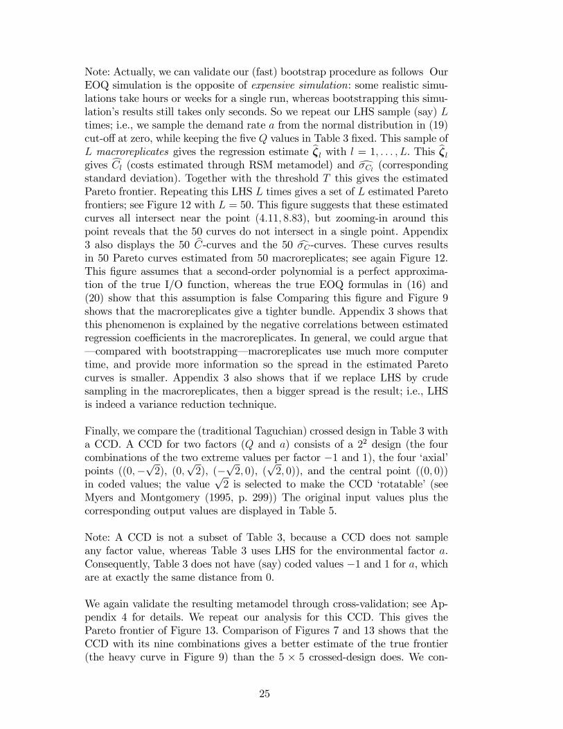
We again validate the resulting metamodel through cross-validation; see Ap-pendix 4 for details. We repeat our analysis for this CCD. This gives thePareto frontier of Figure 13. Comparison of Figures 7 and 13 shows that theCCD with its nine combinations gives a better estimate of the true frontier(the heavy curve in Figure 9) than the 5 � 5 crossed-design does. We con-
25

4.1 4.11 4.12 4.13 4.14 4.15 4.16 4.17 4.18 4.19 4.2
x 104
8.74
8.76
8.78
8.8
8.82
8.84
8.86
8.88
8.9x 10
4
s(C)
E(C
)
Cσ
C
4.1 4.11 4.12 4.13 4.14 4.15 4.16 4.17 4.18 4.19 4.2
x 104
8.74
8.76
8.78
8.8
8.82
8.84
8.86
8.88
8.9x 10
4
s(C)
E(C
)
Cσ
C
Fig. 12. Pareto frontiers estimated from 50 macroreplicates, and true frontier (dottedcurve)
Q a C
19393.40 5559.67 61945.81
19393.40 10529.69 114721.4
40606.60 5559.67 63330.64
40606.60 10529.69 114499.6
15000 8044.68 89132.55
45000 8044.68 89342.05
30000 4530.34 51615.54
30000 11559.02 124713.8
30000 8044.68 88164.67Table 5I/O simulation data for EOQ model with CCD design
jecture that the bigger design gives a more accurate OLS estimator b� of thewrong (misspeci�ed) metamodel (namely, a second-order polynomial) for thetrue I/O function implied by the EOQ simulation model.
26
Fig. 13. Bootstrapped Pareto frontiers, original estimated frontier (dashed curve)and true Pareto frontier (heavy curve) based on CCD
5 Conclusions and future research
This article leads to the following conclusions:
(1) Robust optimization of simulated systems may use Taguchi�s worldview,which distinguishes between decision variables to be optimized and envi-ronmental variables that remain uncertain.
(2) Taguchi�s statistical techniques may be replaced by RSM.(3) Myers and Montgomery (1995)�s RSM developed for Taguchian optimiza-
tion may be further adapted such that it results in bootstrapped Paretofrontiers, which better enable management to make the �nal compromisedecision.
(4) Application of this new methodology to the classic EOQ model showsthat� for a certain (known) environment� the methodology gives a goodestimate of the true EOQ, and� for an environment with a demand ratethat has a known distribution� the classic EOQ and the robust EOQdi¤er.
Future research may address the following issues.
� We conjectured that the bigger crossed design gave a more accurate OLSestimator b� of a misspeci�ed metamodel. This is a good reason for usinga better type of metamodel, namely a Kriging model (Generalized Linear
27
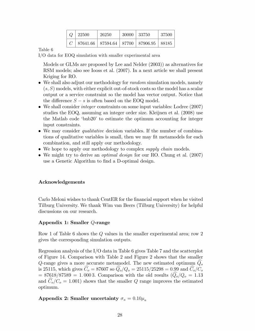
Q 22500 26250 30000 33750 37500
C 87641.66 87594.64 87700 87906.95 88185Table 6I/O data for EOQ simulation with smaller experimental area
Models or GLMs are proposed by Lee and Nelder (2003)) as alternatives forRSM models; also see Iooss et al. (2007). In a next article we shall presentKriging for RO.
� We shall also adjust our methodology for random simulation models, namely(s; S) models, with either explicit out-of-stock costs so the model has a scalaroutput or a service constraint so the model has vector output. Notice thatthe di¤erence S � s is often based on the EOQ model.
� We shall consider integer constraints on some input variables: Lodree (2007)studies the EOQ, assuming an integer order size. Kleijnen et al. (2008) usethe Matlab code �bnb20�to estimate the optimum accounting for integerinput constraints.
� We may consider qualitative decision variables. If the number of combina-tions of qualitative variables is small, then we may �t metamodels for eachcombination, and still apply our methodology.
� We hope to apply our methodology to complex supply chain models.� We might try to derive an optimal design for our RO. Chung et al. (2007)use a Genetic Algorithm to �nd a D-optimal design.
Acknowledgements
Carlo Meloni wishes to thank CentER for the �nancial support when he visitedTilburg University. We thank Wim van Beers (Tilburg University) for helpfuldiscussions on our research.
Appendix 1: Smaller Q-range
Row 1 of Table 6 shows the Q values in the smaller experimental area; row 2gives the corresponding simulation outputs.
Regression analysis of the I/O data in Table 6 gives Table 7 and the scatterplotof Figure 14. Comparison with Table 2 and Figure 2 shows that the smallerQ-range gives a more accurate metamodel. The new estimated optimum cQois 25115, which gives cCo = 87607 so cQo=Qo = 25115=25298 = 0:99 and cCo=Co= 87618=87589 = 1: 000 3. Comparison with the old results (cQo=Qo = 1.13and cCo=Co = 1.001) shows that the smaller Q range improves the estimatedoptimum.
Appendix 2: Smaller uncertainty �a = 0:10�a
28
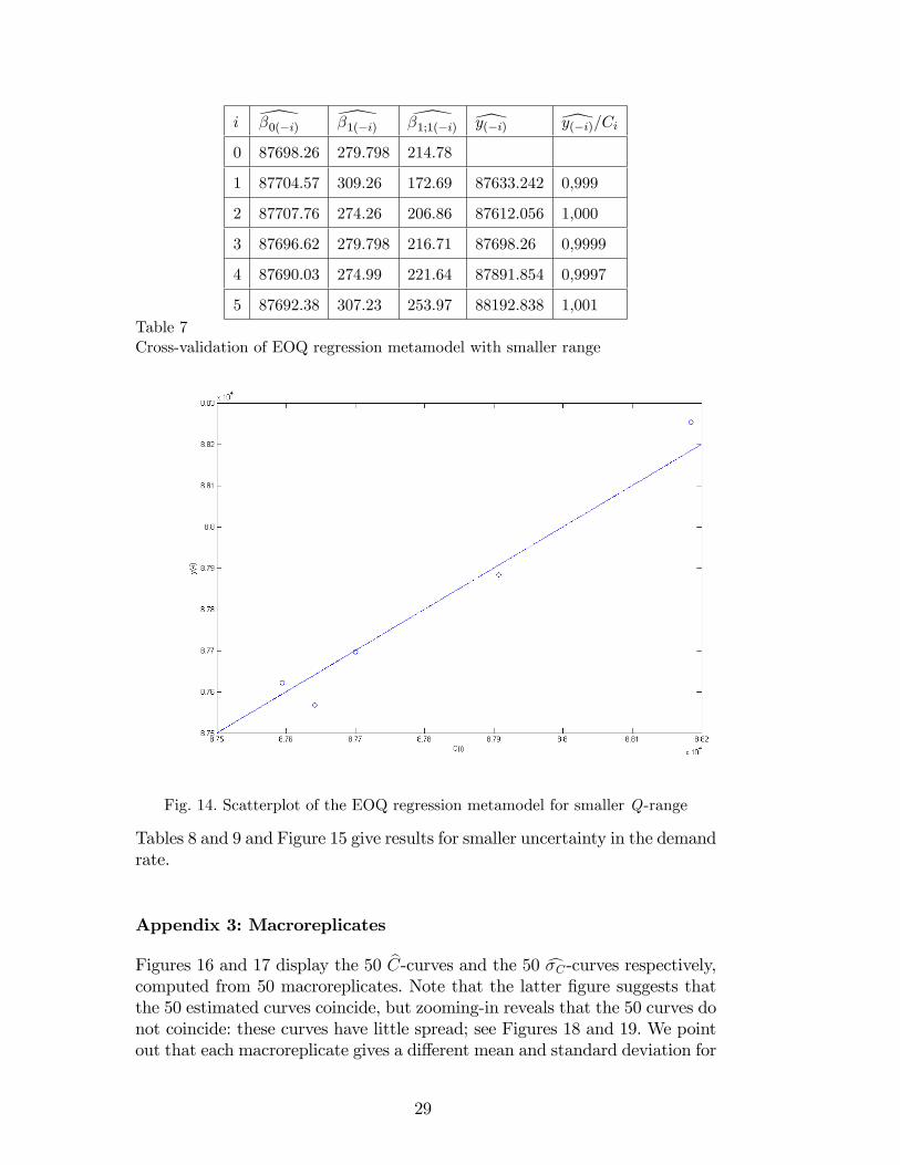
i \�0(�i) \�1(�i) \�1;1(�i) [y(�i) [y(�i)=Ci
0 87698.26 279.798 214.78
1 87704.57 309.26 172.69 87633.242 0,999
2 87707.76 274.26 206.86 87612.056 1,000
3 87696.62 279.798 216.71 87698.26 0,9999
4 87690.03 274.99 221.64 87891.854 0,9997
5 87692.38 307.23 253.97 88192.838 1,001Table 7Cross-validation of EOQ regression metamodel with smaller range
Fig. 14. Scatterplot of the EOQ regression metamodel for smaller Q-range
Tables 8 and 9 and Figure 15 give results for smaller uncertainty in the demandrate.
Appendix 3: Macroreplicates
Figures 16 and 17 display the 50 bC-curves and the 50 c�C-curves respectively,computed from 50 macroreplicates. Note that the latter �gure suggests thatthe 50 estimated curves coincide, but zooming-in reveals that the 50 curves donot coincide: these curves have little spread; see Figures 18 and 19. We pointout that each macroreplicate gives a di¤erent mean and standard deviation for
29
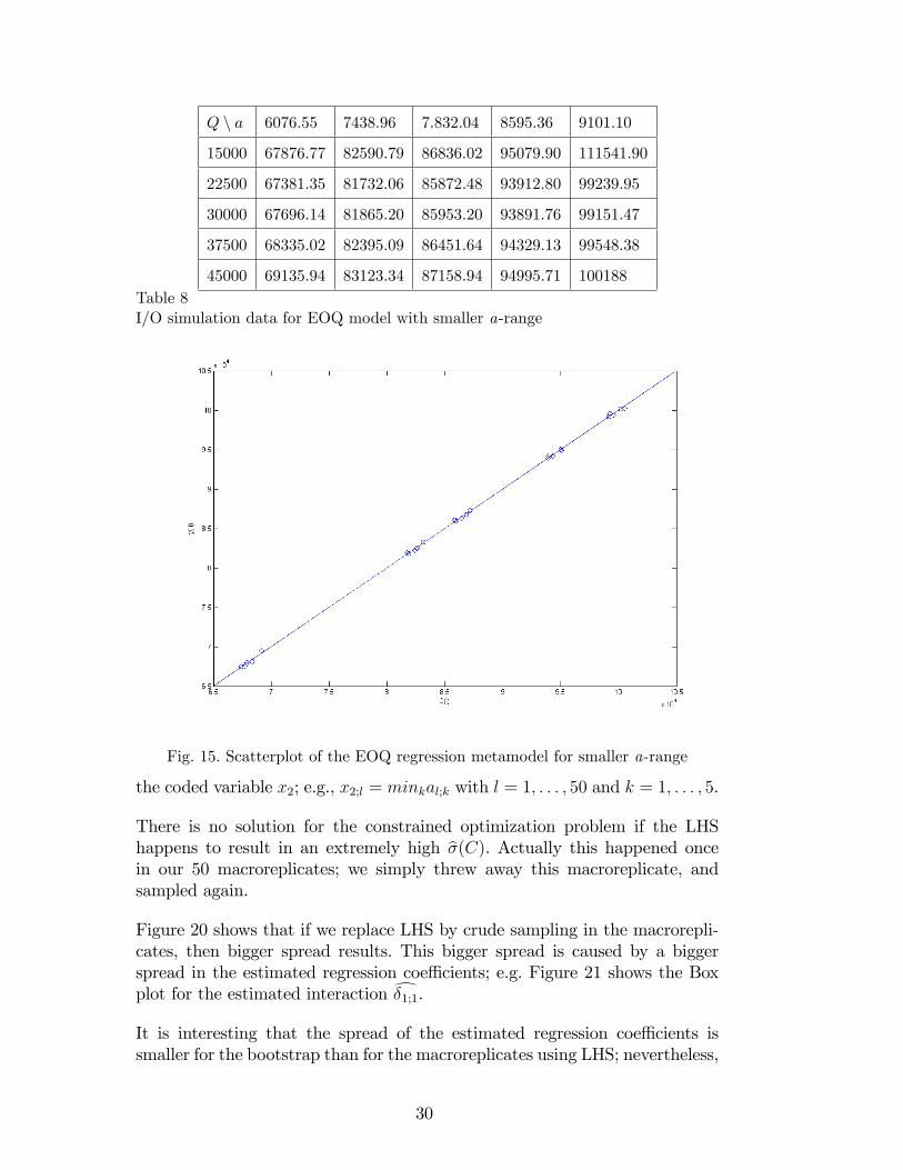
Q n a 6076.55 7438.96 7.832.04 8595.36 9101.10
15000 67876.77 82590.79 86836.02 95079.90 111541.90
22500 67381.35 81732.06 85872.48 93912.80 99239.95
30000 67696.14 81865.20 85953.20 93891.76 99151.47
37500 68335.02 82395.09 86451.64 94329.13 99548.38
45000 69135.94 83123.34 87158.94 94995.71 100188Table 8I/O simulation data for EOQ model with smaller a-range
Fig. 15. Scatterplot of the EOQ regression metamodel for smaller a-range
the coded variable x2; e.g., x2;l = minkal;k with l = 1; : : : ; 50 and k = 1; : : : ; 5.
There is no solution for the constrained optimization problem if the LHShappens to result in an extremely high b�(C). Actually this happened oncein our 50 macroreplicates; we simply threw away this macroreplicate, andsampled again.
Figure 20 shows that if we replace LHS by crude sampling in the macrorepli-cates, then bigger spread results. This bigger spread is caused by a biggerspread in the estimated regression coe¢ cients; e.g. Figure 21 shows the Boxplot for the estimated interaction d�1;1.It is interesting that the spread of the estimated regression coe¢ cients issmaller for the bootstrap than for the macroreplicates using LHS; nevertheless,
30
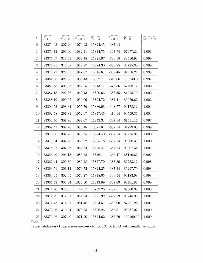
i \�0(�i) \�1(�i) \�1;1(�i) \ 1(�i) \�1;1(�i) [y(�i) [y(�i)=Ci
0 83374.03 307.26 1070.93 15824.45 -387.14
1 83373.72 296.40 1082.41 15814.75 -367.74 67977.23 1.001
2 83375.07 313.61 1062.48 15825.97 -390.18 82516.93 0.999
3 83375.95 316.08 1058.27 15824.30 -386.85 86725.30 0.999
4 83378.77 320.83 1047.87 15815.61 -369.45 94878.21 0.998
5 83382.36 325.08 1036.43 15802.71 -343.66 100240.08 0.997
6 83383.68 300.95 1064.25 15813.17 -375.86 67498.17 1.002
7 83387.18 299.36 1060.43 15820.66 -383.35 81915.79 1.002
8 83388.19 299.02 1059.09 15824.72 -387.41 86079.62 1.002
9 83390.53 298.34 1055.76 15836.08 -398.77 94178.12 1.003
10 83392.58 297.83 1052.67 15847.45 -410.14 99559.36 1.003
11 83353.46 307.26 1092.07 15842.31 -387.14 67511.15 0.997
12 83367.41 307.26 1078.48 15825.81 -387.14 81799.08 0.999
13 83370.36 307.26 1075.25 15824.40 -387.14 85915.31 1.000
14 83375.54 307.26 1069.02 15825.18 -387.14 93908.39 1.000
15 83378.87 307.26 1064.54 15828.47 -387.14 99207.34 1.001
16 83355.49 295.13 1083.75 15846.11 -365.47 68110.62 0.997
17 83362.44 300.30 1080.18 15827.79 -383.80 82233.12 0.998
18 83363.51 301.14 1079.72 15824.25 -387.34 86297.79 0.998
19 83364.95 302.35 1079.27 15818.05 -393.54 94183.08 0.998
20 83365.52 302.94 1079.30 15813.89 -397.69 99401.86 0.999
21 83372.90 346.65 1112.57 15789.26 -457.51 69500.37 1.005
22 83372.29 317.81 1084.94 15821.92 -392.19 83245.96 1.001
23 83372.43 314.61 1081.48 15824.57 -386.90 87251.28 1.001
24 83373.06 310.04 1075.65 15826.26 -383.51 95037.07 1.000
25 83373.96 307.40 1071.20 15824.62 -386.79 100190.39 1.000Table 9Cross-validation of regression metamodel for RO of EOQ with smaller a-range
31
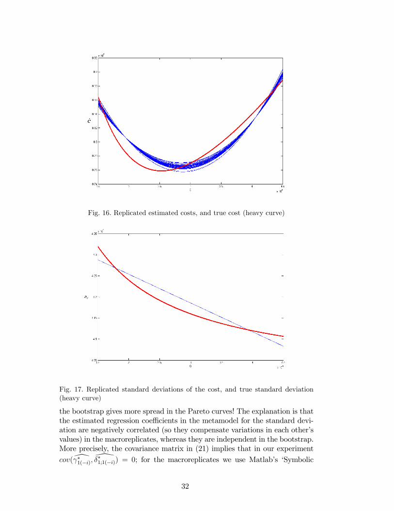
Fig. 16. Replicated estimated costs, and true cost (heavy curve)
Fig. 17. Replicated standard deviations of the cost, and true standard deviation(heavy curve)
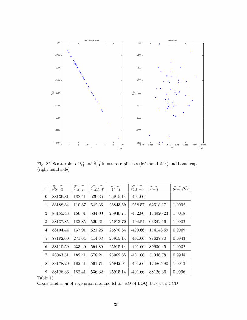
the bootstrap gives more spread in the Pareto curves! The explanation is thatthe estimated regression coe¢ cients in the metamodel for the standard devi-ation are negatively correlated (so they compensate variations in each other�svalues) in the macroreplicates, whereas they are independent in the bootstrap.More precisely, the covariance matrix in (21) implies that in our experiment
cov([ �1(�i); \��1;1(�i)) = 0; for the macroreplicates we use Matlab�s �Symbolic
32
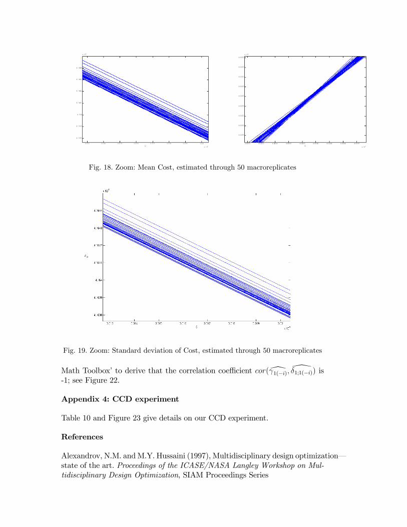
Fig. 18. Zoom: Mean Cost, estimated through 50 macroreplicates
Fig. 19. Zoom: Standard deviation of Cost, estimated through 50 macroreplicates
Math Toolbox�to derive that the correlation coe¢ cient cor([ 1(�i); \�1;1(�i)) is-1; see Figure 22.
Appendix 4: CCD experiment
Table 10 and Figure 23 give details on our CCD experiment.
References
Alexandrov, N.M. andM.Y. Hussaini (1997), Multidisciplinary design optimization�state of the art. Proceedings of the ICASE/NASA Langley Workshop on Mul-tidisciplinary Design Optimization, SIAM Proceedings Series
4.1 4.12 4.14 4.16 4.18 4.2 4.22
x 104
8.72
8.74
8.76
8.78
8.8
8.82
8.84
8.86x 10
4
s(C)
E(C
)
Cσ
C
4.1 4.12 4.14 4.16 4.18 4.2 4.22
x 104
8.72
8.74
8.76
8.78
8.8
8.82
8.84
8.86x 10
4
s(C)
E(C
)
Cσ
C
Fig. 20. Crude sampling: replicated estimated Pareto frontiers
Bootstrap MacroReplicates LHS2400
2200
2000
1800
1600
1400
1200
1000
800
δ 1;1
Fig. 21. Box plot for the estimated interaction �1;1
34
3 4 5 6 7 8 9 10
x 104
2400
2200
2000
1800
1600
1400
1200
1000
800macroreplicates
γ1
δ 1;1
3.66 3.665 3.67 3.675 3.68 3.685 3.69 3.695
x 104
1100
1050
1000
950
900
850
800
750
700bootstrap
γ1
δ 1;1
Fig. 22. Scatterplot ofc 1 andd�1;1 in macro-replicates (left-hand side) and bootstrap(right-hand side)
i \�0(�i) \�1(�i) \�1;1(�i) \ 1(�i) \�1;1(�i) [y(�i) [y(�i)=Ci
0 88136.81 182.41 529.35 25915.14 -401.66
1 88188.84 110.87 542.36 25843.59 -258.57 62518.17 1.0092
2 88155.43 156.81 534.00 25940.74 -452.86 114926.23 1.0018
3 88137.85 183.85 529.61 25913.70 -404.54 63342.16 1.0002
4 88104.44 137.91 521.26 25870.64 -490.66 114143.59 0.9969
5 88182.69 271.64 414.63 25915.14 -401.66 88627.80 0.9943
6 88110.59 233.40 594.89 25915.14 -401.66 89630.45 1.0032
7 88063.51 182.41 578.21 25962.65 -401.66 51346.78 0.9948
8 88178.26 182.41 501.71 25942.01 -401.66 124865.80 1.0012
9 88126.36 182.41 536.32 25915.14 -401.66 88126.36 0.9996Table 10Cross-validation of regression metamodel for RO of EOQ, based on CCD
35
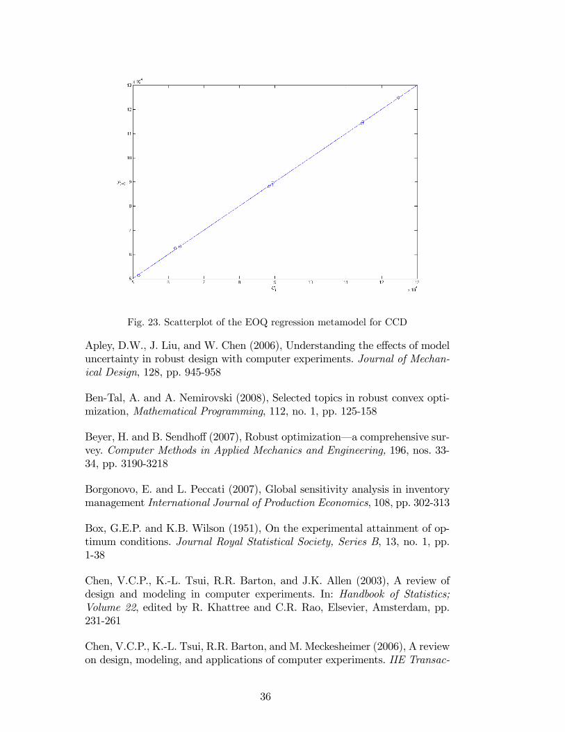
Fig. 23. Scatterplot of the EOQ regression metamodel for CCD
Apley, D.W., J. Liu, and W. Chen (2006), Understanding the e¤ects of modeluncertainty in robust design with computer experiments. Journal of Mechan-ical Design, 128, pp. 945-958
Ben-Tal, A. and A. Nemirovski (2008), Selected topics in robust convex opti-mization, Mathematical Programming, 112, no. 1, pp. 125-158
Beyer, H. and B. Sendho¤ (2007), Robust optimization� a comprehensive sur-vey. Computer Methods in Applied Mechanics and Engineering, 196, nos. 33-34, pp. 3190-3218
Borgonovo, E. and L. Peccati (2007), Global sensitivity analysis in inventorymanagement International Journal of Production Economics, 108, pp. 302-313
Box, G.E.P. and K.B. Wilson (1951), On the experimental attainment of op-timum conditions. Journal Royal Statistical Society, Series B, 13, no. 1, pp.1-38
Chen, V.C.P., K.-L. Tsui, R.R. Barton, and J.K. Allen (2003), A review ofdesign and modeling in computer experiments. In: Handbook of Statistics;Volume 22, edited by R. Khattree and C.R. Rao, Elsevier, Amsterdam, pp.231-261
Chen, V.C.P., K.-L. Tsui, R.R. Barton, and M. Meckesheimer (2006), A reviewon design, modeling, and applications of computer experiments. IIE Transac-
36
tions, 38, pp. 273-291
Chen, W., R. Jin, and A. Sudjianto (2006), Analytical global sensitivity analy-sis and uncertainty propagation for robust design, Journal of Quality Tech-nology, 38, no. 4, pp. 333-348
Chung, P.J., H.B. Goldfarb and D.C. Montgomery (2007), Optimal designsfor mixture-process experiments with control and noise variables, Journal ofQuality Technology, 39, no. 3, pp. 179-190
Darwish, M.A. (2008), EPQ models with varying setup cost. InternationalJournal of Production Economics, 113, no. 1, pp. 297-306
Efron, B. and R.J. Tibshirani (1993), An introduction to the bootstrap. Chap-man & Hall, New York
Greenberg, H.J. and T. Morisson (2008), Robust optimization. OperationsResearch and Management Science Handbook, edited by A.R. Ravindran, CRCPress, Boca Raton, Florida
Hillier, F.S. and G. J. Lieberman (2001), Introduction to Operations Research;seventh edition, McGraw Hill, Boston
Iooss, B., M. Ribatet, and A. Marrel (2007), Global sensitivity analysis ofstochastic computer models with generalized additive models. Working Paper,CEA, Cadarache, Saint Paul lez Durance, France
Kelton, W.D., R.P. Sadowski, and D.T. Sturrock (2007), Simulation withArena; fourth edition. McGraw-Hill, Boston
Kleijnen, J.P.C. (1980), Computers and pro�ts: quantifying �nancial bene�tsof information. Addison-Wesley, Reading, Massachusetts
Kleijnen, J.P.C., (1987), Statistical tools for simulation practitioners. MarcelDekker, New York
Kleijnen, J.P.C. (2008),Design and analysis of simulation experiments, Springer,New York
Kleijnen, J.P.C. and J.C. Helton (1999), Statistical analyses of scatter plots toidentify important factors in large-scale simulations,1: review and comparisonof techniques.Reliability Engineering and Systems Safety, 65, no. 2, pp. 147-185 (also published as Sandia Report SAND98-2202, April 1999)
Kleijnen, J.P.C. and R.G. Sargent (2000), A methodology for the �tting andvalidation of metamodels in simulation. European Journal of Operational Re-search, 120, no. 1, pp. 14-29
37
Kleijnen, J.P.C., W. van Beers, and I. van Nieuwenhuyse (2008), Constrainedoptimization in simulation: novel approach. CentER Discussion Paper, Cen-tER, Tilburg University, Tilburg, the Netherlands
Lee, Y. and J.A. Nelder (2003), Robust design. Journal of Quality Technology,35, no. 1, pp. 2-12
Lodree, E.J. (2007), EOQ revisited: The case of unequal and integral orderquantities. International Journal of Production Economics, 105, no. 2, pp.580-590
Marczyk, J. (2000), Stochastic multidisciplinary improvement: beyond opti-mization. 8th AIAA/NASA/USAF/ISSMO Symposium on MultidisciplinaryAnalysis and Optimization, Long Beach, September 2000, AIAA-2000-4929
Meckesheimer, M., R.R. Barton, T.W. Simpson, and A.J. Booker (2001), Com-putationally inexpensive metamodel assessment strategies. AIAA Journal, 40.no. 10, pp. 2053-2060
Mula, J., R. Poler, J.P. García-Sabater, and F.C. Lario (2006), Models forproduction planning under uncertainty : A review. International Journal ofProduction Economics, 103, no. 1, pp. 271-285
Mulvey, J.M., R.J. Vanderbei, and S.A. Zenios (1995), Robust optimizationof large-scale systems. Operations Research, 43, no. 2, pp. 264-281
Myers, R.H. and D.C. Montgomery (1995), Response surface methodology:process and product optimization using designed experiments.Wiley, New York
Oden, J.T., Chair (2006), Revolutionizing engineering science through simula-tion. National Science Foundation (NSF), Blue Ribbon Panel on Simulation-Based Engineering Science
Park, G-J., T-H. Lee, K.H. Lee, and K-H. Hwang (2006), Robust design: anoverview. AIAA Journal, 44, no. 1, pp. 181-191
Pentico, D.W., M.J. Drake, and C. Toews (2008), The deterministic EPQ withpartial backordering: a new approach. Omega, in press
Sahinidis, N.V. (2004), Optimization under uncertainty: state-of-the-art andopportunities. Computers and Chemical Engineering, 28, pp. 971-983
Simpson, T.W., J. Peplinski, P.N. Koch, and J.K. Allen (2001), Metamodelsfor computer-based engineering design: survey and recommendation. Engi-neering with Computers, 17, no. 2, pp. 129-150
38
Stinstra, E. and D. den Hertog (2007), Robust optimization using computerexperiments. European Journal of Operational Research, in press
Taguchi, G. (1987), System of experimental designs, volumes 1 and 2. UNIPUB/Krauss International, White Plains, New York
Teng, J-T. (2008), A simple method to compute economic order quantities.European Journal of Operational Research, in press
The MathWorks Inc. (2005), Statistics Toolbox, Natick, Massachusetts
Wu, C.F.J. and M. Hamada (2000), Experiments; planning, analysis, and pa-rameter design optimization. Wiley, New York
Wu. J., J. Li, S. Wang and T.C.E. Cheng (2008), A note on mean-varianceanalysis of the newsvendor model with stockout cost Omega, in press
Yu, G. (1997), Robust economic order quantity models. European Journal ofOperational Research, 100, no. 3, pp. 482-493
Zipkin, P.H. (2000), Foundations of Inventory Management, McGraw-Hill
Vitae
Dellino graduated cum laude in Computer Science Engineering at the Po-litecnico di Bari, Italy, in 2005. Since 2006 she is a Ph.D. student in AppliedMathematics at the University of Bari. She took part in research projectsfunded by academic organizations and companies. Her main research interestsare optimization models and methods, computer simulation methodologies,and Multidisciplinary Design Optimization. She is a member of INFORMS.She is currently visiting the CentER Graduate School, at Tilburg University.
Kleijnen is Professor of �Simulation and Information Systems�at Tilburg Uni-versity. He is a member of the �Department of Information Management�andthe �Operations Research�group of CentER. He also teaches at the EindhovenUniversity of Technology, namely the course called �Simulation for logistics�for the Postgraduate International Program in Logistics Management Sys-tems. His research concerns simulation (especially its statistical design andanalysis), information systems, and supply chains. He has been a consul-tant for several organizations in the USA and Europe. He serves on manyinternational editorial boards and scienti�c committees. He spent some yearsin the USA, at universities and private companies. He received a numberof national and international awards. More details are given on his website(http://center.uvt.nl/sta¤/kleijnen/).
39
Meloni got a Ph.D. in Operations Research from La Sapienza University ofRome in 2000. Then he joined the Università degli Studi Roma Tre as post-doctoral fellow in Operations Research. In July 2002 he became AssistantProfessor of Systems Engineering at the Politecnico di Bari. He participatedin several research projects funded by various academic organizations andcompanies. His main research interests concern applications of optimizationand other OR/MS methodologies to Multidisciplinary Systems Design, Sup-ply Chain Management, Advanced Planning & Scheduling, and Health CareService Operations Management. He presented his reserach at several inter-national conferences, and published in various international journals. He is amember of the Italian Society of Operations Research (AIRO) and INFORMS.
40