tilburg university robust optimization methods for chance
TRANSCRIPT

Tilburg University
Robust optimization methods for chance constrained, simulation-based, and bilevelproblemsYanikoglu, I.
Publication date:2014
Document VersionPublisher's PDF, also known as Version of record
Link to publication in Tilburg University Research Portal
Citation for published version (APA):Yanikoglu, I. (2014). Robust optimization methods for chance constrained, simulation-based, and bilevelproblems. CentER, Center for Economic Research.
General rightsCopyright and moral rights for the publications made accessible in the public portal are retained by the authors and/or other copyright ownersand it is a condition of accessing publications that users recognise and abide by the legal requirements associated with these rights.
• Users may download and print one copy of any publication from the public portal for the purpose of private study or research. • You may not further distribute the material or use it for any profit-making activity or commercial gain • You may freely distribute the URL identifying the publication in the public portal
Take down policyIf you believe that this document breaches copyright please contact us providing details, and we will remove access to the work immediatelyand investigate your claim.
Download date: 08. Dec. 2021

Robust Optimization Methods forChance Constrained,
Simulation-Based, and BilevelProblems
Proefschrift
ter verkrijging van de graad van doctor aan Tilburg Universityop gezag van de rector magnificus, prof.dr. Ph. Eijlander,in het openbaar te verdedigen ten overstaan van een doorhet college voor promoties aangewezen commissie in de RuthFirst zaal van de Universiteit op dinsdag 2 september 2014om 14.15 uur door
Ihsan Yanıkoglu
geboren op 4 augustus 1985 te Izmir, Turkije

Promotiecommissie:
Promotor: prof.dr.ir. Dick den Hertog
Copromotor: dr. Daniel Kuhn
Overige leden: prof.dr. Aharon Ben-Talprof.dr. Etienne de Klerkprof.dr. Goos Kantdr. Ruud Brekelmansdr. Juan Vera Lizcano
Robust Optimization Methods for Chance Constrained, Simulation-Based, and Bilevel Problems
Copyright c© 2014 Ihsan Yanıkoglu
All rights reserved.
No part of this book may be reproduced, stored in a retrieval system, or transmitted inany form or by any means, electronic, mechanical, photocopying, recording, or otherwise, withoutwritten permission from the author.

Acknowledgements
I would like to express my most sincere thanks to my supervisor Dick den Hertog. Heis one of the most influential people I have met in my entire life, who truly changedit in many different ways. I would like to thank him once more for everything he hasmade at all stages of my life in Tilburg.
I would like to thank Daniel Kuhn for giving me the opportunity to work with himin the final year of my Ph.D. and accepting to co-supervise my thesis. I also expressmy gratitude to him and his colleagues in EPFL for the friendly environment theyhave created during my three months stay in Lausanne.
I thank to my co-authors Jack Kleijnen and Bram Gorissen for their valuable com-ments and discussions during the realization of the two chapters in this thesis.
A special mention goes to Gul Gurkan who approved my application to Tilburg Uni-versity in 2009, and arranged everything in the first two years.
I would like to thank CentER Research Institute for their financial support through-out my studies. CentER made everything easier for me in the past five years.
I thank committee members Aharon Ben-Tal, Etienne de Klerk, Goos Kant, RuudBrekelmans, and Juan Vera Lizcano for accepting to read and review this thesis.
Finally, I would like to thank to my family for their everlasting support and love.
Ihsan YanıkogluTilburg, June 2014

ii
Contents
1 Introduction 11.1 Optimization Under Uncertainty 21.2 Robust Optimization 61.3 Adjustable Robust Optimization 91.4 Contribution and Overview 121.5 Disclosure 14
2 Hints for Practical Robust Optimization 172.1 Introduction 172.2 Recipe for Robust Optimization in Practice 192.3 Choosing Uncertainty Set 272.4 Linearly Adjustable Robust Counterpart: Linear in What? 302.5 Adjustable Integer Variables 312.6 Binary Variables in Big-M-Constraints are Automatically Adjustable 362.7 Robust Counterparts of Equivalent Deterministic Problems are not
Necessarily Equivalent 382.8 How to Deal with Equality Constraints? 432.9 On Maximin and Minimax Formulations of RC 452.10 Quality of Robust Solution 472.11 RC May Take Better “Here and Now” Decisions than AARC 512.12 Conclusion 56
3 Safe Approximations of Ambiguous Chance Constraints 603.1 Introduction 603.2 Introduction to φ-Divergence and Confidence Sets 64
3.2.1 Confidence Sets Based on φ-Divergence 643.2.2 Probability Bound for Subset of Cells 66
3.3 Safe Approximation Method 693.3.1 General Setup 693.3.2 Algorithm 71

iii
3.3.3 Extensions 763.4 Experimental Results 78
3.4.1 Illustrative Example 793.4.2 Optimization of Cross-Docking Distribution Center 813.4.3 Optimizing Color Picture Tube 86
3.5 Conclusions 903.6 Derivation of Robust Counterpart 913.7 Data and Additional Results 92
3.7.1 Extra Results for Example 4.1 923.7.2 Example 4.3 93
3.8 Additional Experiments 943.8.1 Comparison with Randomized Approach 943.8.2 Comparison with One-by-One Approach 963.8.3 Multi-Period Work Scheduling Problem 963.8.4 Dependent Data Set and Data Set of Example 4.4 100
4 Adjustable Robust Optimization Using Metamodels 1054.1 Introduction 1054.2 Robust Parameter Design 1104.3 Robust Optimization with Unknown Distributions 112
4.3.1 Uncertainty Sets 1124.3.2 Robust Counterparts of Mean and Variance 1134.3.3 Alternative Metamodels and Risk Measures 117
4.4 Adjustable Robust Optimization 1204.5 Realistic Examples 127
4.5.1 Television Images 1284.5.2 Distribution Center 132
4.6 Conclusions and Future Research 135
5 Robust Pessimistic Bilevel Optimization 1395.1 Introduction 1395.2 Single-Level Reformulation 1425.3 Primal and Dual Linear Decision Rules 143
5.3.1 Primal Approximation 1445.3.2 Dual Approximation 145
5.4 Robust Bilevel Optimization 1475.5 Conclusion 154

CHAPTER 1
Introduction
Robust optimization (RO) is a young and active research field that has been mainlydeveloped in the course of last fifteen years. For a quick overview of the associatedliterature, we refer to the survey papers by Ben-Tal and Nemirovski (2002); Bertsi-mas et al. (2011); Beyer and Sendhoff (2007). Additional details on the history ofRO that is in line with the research of this thesis shall be discussed in later chapters.
RO is well-known because it yields computationally tractable methods for uncer-tain optimization problems. Unlike its counterparts, i.e., dynamic and stochasticprogramming, it does not suffer from the curse of dimensionality. However, despiteall its computational advantages, it is remarkable that practical use of RO in real-life is still lagging behind. This is mainly because of some issues and shortcomingsthat hinder successful applications of RO in real-life. In this thesis, our goal is toovercome some of these shortcomings and to help practitioners for successfully ap-plying RO in practice. In the next chapter, several practical topics are discussed inseparate sections. In addition, a practical guide, that shows a roadmap on how toapply RO in practice, is given. In the remaining chapters of the thesis, we proposeand analyze tractable RO methodologies for several classes of optimization problems.
In this chapter, we give a brief introduction on optimization under uncertainty, aswell as the contributions of our research and the overview of the following chapters.Section 1.1 describes the sources of uncertainties in mathematical optimization prob-lems and the optimization techniques to deal with these uncertainties. Section 1.2gives a brief introduction on RO. Section 1.3 describes the concept of adjustable RO.Section 1.4 discusses the contribution of this thesis.

Optimization Under Uncertainty 2
1.1 Optimization Under UncertaintyMathematical optimization problems often have uncertainty in problem parametersbecause of measurement/rounding, estimation/forecasting, or implementation errors.We describe these errors in detail below.
Measurement/rounding errors are often caused when an actual measurement isrounded to a nearest value according to a rule, e.g., the nearest tenth or hundredth,or when the actual value of the parameter cannot be measured with a high precisionas it appears in reality. For example, if the reported parameter value is 9.5 accordingto the nearest tenth, then the actual value can be anywhere between 9.45 and 9.55,i.e., it is uncertain.
Estimation/forecasting errors come from the lack of true knowledge about theproblem parameter or the impossibility to estimate the true characteristics of theactual data. For example, demand and cost parameters are often subject to suchestimation/forecasting errors.
Implementation errors are often caused by “ugly” reals that can be hardly imple-mented with the same precision in reality. For example, suppose the optimal voltagein a circuit, that is calculated by an optimization tool, is 2.782169. The decimal partof this optimal solution can be hardly implemented in practice, since you cannotprovide the same precision.
Optimization based on nominal values often lead to “severe” infeasibilities. No-tice that a small uncertainty in the problem data can make the nominal solutioncompletely useless. A case study in Ben-Tal and Nemirovski (2000) shows that per-turbations as low as 0.01% in problem coefficients result constraint violations morethan 50% in 13 out of 90 NETLIB Linear Programming problems considered in thestudy. In 6 of this 13 problems violations were over 100%, where 210,000% beingthe highest (i.e., seven scale higher than the tested uncertainty). Therefore, a practi-cal optimization methodology that proposes immunity against uncertainty is neededwhen the uncertainty heavily affects the quality of the nominal solution.
Illustrative example on flaw of using nominal values. Consider an uncertainlinear optimization problem with a single constraint:
a>x ≤ b, (1.1)
where a = a + ρζ is the vector of uncertain coefficients and a being the nominal

Optimization Under Uncertainty 3
vector, ζ ∈ R2 is the uncertain parameter that is uniformly distributed in a unit box||ζ||∞ ≤ 1, and ρ is a scalar shifting parameter. Now (say) we ignore the uncertaintyin the constraint coefficients and solve the associated problem according to the nom-inal data, i.e., a = a, and assume that the constraint is binding for the associatednominal optimal solution x, i.e., ax = b. Figure 1.1 shows the original constraint[a>x ≤ b] in the uncertainty space when x is fixed to the nominal optimal solutionx.
Figure 1.1 – Feasible region of the uncertain constraint (a+ρζ)>x ≤ b in theuncertainty space [−1, 1]2.
The solid line in Figure 1.1 represents ζ values where the uncertain constraint isbinding when x is fixed to the nominal solution x, and the dashed lines represent thefeasible uncertainty region for the same constraint. Therefore, the area that is deter-mined by the intersection of the unit box with the dashed region gives the subset forwhich the nominal x is robust. From the figure we can conclude that the probabilityof violating this constraint can be as high as 50%, since ζ follows a uniform distri-bution. This shows that uncertainty may severely affect the quality of the nominalsolution, and there exists a crucial need for an optimization methodology that yieldssolutions that are immunized against the uncertainty.
Now let us consider the following figure that presents another illustrative example.In Figure 1.2, there are three constraints and their binding values are representedby the solid lines. The constraint on the right-hand side is uncertain, and the othertwo are certain. For the uncertain constraint, the solid line represents the binding

Optimization Under Uncertainty 4
Figure 1.2 – Effects of uncertainty on feasibility and optimality performanceof solutions (this figure is represented in the decision variable space).
value of the constraint for the nominal data and the dashed line represents the samefor a different realization of the uncertain data. Notice that, different than in Figure1.1, in Figure 1.2 we are in the space of the decision variable x. We assume thatthe problem at hand is an uncertain linear problem, therefore, the optimal solutionsare obtained at the extreme points of the feasible region where the constraints arebinding. Suppose x1 denotes the unique nominal optimal solution of the problem.It is easy to see that x1 may be highly infeasible when the associated constraint isuncertain. The new (robust) optimal solution may become x3. Now consider the casewhere x1 and x2 are both optimal for the nominal data, i.e., the optimal facet is theline segment that connects x1 and x2. In this case, the decision maker would alwaysprefer x2 over x1, since its feasibility performance is less affected by the uncertainty.This shows that staying away from “risky” solutions that have uncertain bindingconstraints may be beneficial.
There are two complementary approaches in optimization that deals with data un-certainty, namely, RO and stochastic optimization (SO). Each method has its ownassumptions. To begin with, basic SO has the following assumptions (Ben-Tal et al.,2009, p. xiii):
S.1. The underlying probability distribution or a restricted family of distributionsof the uncertain parameter must be known.
S.2. The associated family of distributions or the distribution should not changeover the considered time horizon that the decisions will be made.
S.3. The decision maker should be ready to accept probabilistic guarantees as theperformance measure against the uncertainty.
If these conditions are met and the deterministic counterpart of the stochastic prob-lem is tractable, then SO is the right optimization methodology to solve the problem

Optimization Under Uncertainty 5
at hand. For additional details on SO we refer to Prekopa (1995); Birge and Lou-veaux (2011); Shapiro and Ruszczynski (2003), and Charnes and Cooper (1959).
On the other hand, the “basic” RO approach has the following three implicit assump-tions (Ben-Tal et al., 2009, p. xii):
R.1. All decision variables represent “here and now” decisions: they should get spe-cific numerical values as a result of solving the problem before the actual data“reveals itself”.
R.2. The decision maker is fully responsible for consequences of the decisions to bemade when, and only when, the actual data is within the prespecified uncer-tainty set.
R.3. The constraints of the uncertain problem in question are “hard” – the deci-sion maker cannot tolerate violations of constraints when the data is in theprespecified uncertainty set.
It is important to point out that assumption [R.1] can be alleviated by adjustablerobust optimization (ARO); a brief introduction on ARO will also be given in Section1.3, but details will follow in Chapters 4 & 5. In addition, assumption [R.3] can bealleviated by globalized robust optimization (Ben-Tal et al., 2009, Ch. 3 & 11), aswell as by using safe approximations of chance constraints that shall be discussed inChapter 3.
If we compare the basic versions of RO and SO, the latter seems to be less conser-vative than the former since it is not worst-case oriented. However, it is importantto point out that the SO approach is valid only when the probability distribution isknown. Notice that RO does not have such a restriction since it works with uncer-tainty sets that can be derived by expert opinion or using historical data. Moreover,the RO paradigm is computationally more tractable than the SO approach; for de-tails on such examples we refer to Chapter 3, Ben-Tal et al. (2009, pp. xiii - xv), andChen et al. (2006). It is important to point out that, although this thesis is based onRO, some chapters are closely related to SO, e.g., Chapter 3 deals with safe approx-imations of ambiguous chance constraints, and such ambiguous chance constraintscan also be analyzed in the SO approach, and Chapter 5 proposes stochastic androbust reformulations of a class of bilevel optimization problems. Chapter 3 showshow SO and RO may substitute each other according to different sets of assumptionson the uncertainty; and Chapter 5 shows how the two approaches may complement

Robust Optimization 6
each other under mild assumptions on the uncertainty.
As mentioned before, this thesis is based on the RO paradigm and we devote aseparate section on RO below.
1.2 Robust Optimization
“A specific and relatively novel methodology for handling mathematicaloptimization problems with uncertain data” Ben-Tal et al. (2009)
The objective of RO is to find solutions that are robust to the uncertainty of pa-rameters in a mathematical optimization problem. It requires that the constraintsof a given problem should be satisfied for all realizations of the uncertain parametersin a so-called uncertainty set. The robust version of a mathematical optimizationproblem is generally referred to as the robust counterpart (RC) problem. Below wepresent the RC of an uncertain linear optimization problem:
maxxc>x : Ax ≤ b ∀A ∈ U, (1.2)
where x ∈ Rn are the decision variables, c ∈ Rn are the certain cost coefficients,b ∈ Rn is the certain constraint right-hand side, A ∈ Rm×n denotes an uncertainmatrix that resides in a given uncertainty set U, and the constraints should be sat-isfied for all the uncertainty in U. In RO we may assume without loss of generalitythat: 1) the objective is certain; 2) the constraint right-hand side is certain; 3) U iscompact and convex; and 4) the uncertainty is constraint-wise.
Below, we explain the technical reasons of why the above stated four “basic” ROassumptions are not restrictive.
E.1. Suppose the objective coefficients (c) of the optimization problem (1.2) areuncertain and (say) these coefficients reside in the uncertainty set C:
maxx
minc∈Cc>x : Ax ≤ b ∀A ∈ U.
Without loss of generality we may assume that the uncertain objective of theoptimization problem can be equivalently reformulated as certain:
maxx∈X ,t
t : t− c>x ≤ 0 ∀c ∈ C, Ax ≤ b ∀A ∈ U,
using an epigraphic reformulation and the additional variable t ∈ R.

Robust Optimization 7
E.2. The second assumption is trivial because the uncertain right-hand side of aconstraint can always be translated to the left-hand side by introducing anextra variable xn+1 = 1.
E.3. The uncertainty set U can be replaced by its convex hull conv(U) in (1.2),because testing the feasibility of a solution with respect to U is equivalent tomaximizing a linear constraint over U, and it yields the same optimal objectivevalue if the constraint is maximized over conv(U). For details of the formalproof and the compactness assumption, see (Ben-Tal et al., 2009, pp. 12–13).
E.4. To illustrate that robustness with respect to U can be formulated constraint-wise, consider a problem with two constraints and with uncertain right-handsides b1 and b2: x1 + b1 ≤ 0, x2 + b2 ≤ 0. Let U = b ∈ R2|b1 ≥ 0, b2 ≥0, b1 + b2 ≤ 1 be the uncertainty set, and U1 = b1 ∈ R|0 ≤ b1 ≤ 1 andU2 = b2 ∈ R|0 ≤ b2 ≤ 1 are the projections of U on b1 and b2. It is easyto see that robustness of the i-th constraint with respect to U is equivalentto robustness with respect to Ui, i.e., the uncertainty in the problem data canbe modelled constraint-wise. For the general proof, see (Ben-Tal et al., 2009,pp. 11–12).
For uncertain nonlinear optimization problems, excluding the third basic assump-tion [E.3], the other three assumptions [E.1], [E.2], and [E.4] are also without loss ofgenerality.
Computational complexity. Notice that (1.2) has infinitely many constraints withfinite number of variables, i.e., it is a semi-infinite optimization problem. Therefore,(1.2) is a computationally challenging problem to be solved in its current version.RO is popular because it proposes computationally tractable reformulations of suchsemi-infinite optimization problems for many classes of uncertainty sets and problemtypes (including several classes of nonlinear optimization problems).
There are three important steps to derive the associated tractable RC. We shall ex-plicitly go through these three steps below. For the sake of exposition we shall focuson an uncertain linear optimization problem with a polyhedral uncertainty set, butthe associated procedure can be applied for other uncertainty sets and problem typesas well.
Three steps to derive tractable RC. As it is mentioned above, the uncertainty

Robust Optimization 8
is constraint-wise in RO, and hence we may focus on a single constraint
(a+Bζ)>x ≤ β ∀ζ ∈ Z, (1.3)
where ζ ∈ Rk is the “primitive” uncertain parameter residing in the polyhedral un-certainty set Z = ζ : Dζ + d ≥ 0. In the left-hand side of (1.3), we use a factormodel to formulate the general uncertain parameter aζ as an affine function a+ Bζ
of the primitive uncertainty ζ (i.e., aζ := a+Bζ). To point out, the dimension of thegeneral uncertain parameter aζ is often much higher than that of the primitive un-certainty ζ. Notice that (1.3) is equivalent to the following worst-case reformulation:
Step 1 (Worst-case): a>x+ maxζ: Dζ+d≥0
(B>x)>ζ ≤ β. (1.4)
Then we take the dual of the inner maximization problem in (1.4). Notice that bystrong duality the inner maximization problem and its dual yield the same optimalobjective value. Therefore, (1.4) is equivalent to
Step 2 (Duality): a>x+ minyd>y : D>y = −B>x, y ≥ 0 ≤ β. (1.5)
It is important to point out that we can also omit the minimization term in (1.5),since it yields an upper bound for the maximization problem in (1.4). Hence, thefinal formulation of the RC becomes
Step 3 (RC): ∃ y : a>x+ d>y ≤ β, D>y = −B>x, y ≥ 0. (1.6)
Note that the constraints in (1.6) are linear in x and y. A similar procedure can alsobe applied to derive the RCs for different classes of uncertainty sets and problemtypes; for additional details on deriving the tractable RCs we refer to Ben-Tal et al.(2009, 2014).
Table 1.1 taken from Ben-Tal et al. (2014) presents the tractable robust counterpartsof an uncertain linear optimization problem for different classes of uncertainty sets.These robust counterparts are derived using the three step procedure that is describedabove, however, we need conic duality instead of LP duality in Step 2 to derive thetractable robust counterparts for the ellipsoidal and the conic uncertainty sets; seethe second and the fourth rows of Table 1.1. Similarly, to derive the tractable RCin the fifth row of Table 1.1, we need Fenchel duality in Step 2; see Rockafellar(1997) for details on Fenchel duality, and Ben-Tal et al. (2014) for the formal proofof the associated RC reformulation. Notice that each RC constraint has a positivesafe guard in the constraint left-hand side, e.g., ρ‖B>x‖1, ρ‖B>x‖2, and d>y; see

Adjustable Robust Optimization 9
Table 1.1 – Tractable Robust Counterparts of [(a+Bζ)>x ≤ β ∀ζ ∈ Z]for different choices of the uncertainty set Z
Uncertainty region Z Robust Counterpart Tractability
Box ‖ζ‖∞ ≤ ρ a>x+ ρ‖B>x‖1 ≤ β LP
Ball/ellipsoidal ‖ζ‖2 ≤ ρ a>x+ ρ‖B>x‖2 ≤ β CQP
Polyhedral Dζ + d ≥ 0
a>x+ d>y ≤ β
D>y = −B>xy ≥ 0
LP
Cone (closed, convex, pointed) Dζ + d ∈ K
a>x+ d>y ≤ β
D>y = −B>xy ∈ K∗
Conic Opt.
Convex functions
hk(ζ) ≤ 0k = 1, . . . , k
(∗)
a>x+∑
k uk h∗(wk
uk),∑
k wk = B>x,
u ≤ 0Convex Opt.
(∗) h∗ denotes the convex conjugate function, i.e, h∗(x) = supyx>y − h(y)
the tractable RCs in the third column of Table 1.1. These safe guards represent thelevel of robustness that we introduce to the constraints. We refer to Ben-Tal et al.(2009, pp. 373–388) and Ben-Tal et al. (2014) for the tractable RCs reformulationsof several classes of uncertain nonlinear optimization problems. Also see, Gorissenet al. (2014) who propose a method that is based on the optimistic dual reformulationwith respect to the full uncertain problem (1.2).
1.3 Adjustable Robust OptimizationAs it is stated in Section 1.2, the basic assumption [R.1] (p. 116), can be alleviatedby adjustable robust optimization (ARO). Different than the “classic” RO that mod-els decision variables as “here and now”, in ARO decision variables can also be “waitand see” that depends on the data revealing itself before the decision is made. Forexample, in a multistage uncertain optimization problem, a decision that is made atperiod t may depend on the data that reveals itself before at time 1, . . . , t− 1. AROadopts decision rules to model the associated dependence between the data and thedecisions.

Adjustable Robust Optimization 10
Adjustable robust counterpart (ARC). Consider a general uncertain linear op-timization problem
minx,yc>ζ x+ d>y : Aζx+By ≤ β : ζ ∈ Z, (1.7)
where x ∈ Rn and y ∈ Rl are the decision vectors; ζ ∈ Rk is the uncertain parameter,cζ ∈ Rn and Aζ ∈ Rm×n are the uncertain coefficients that are affine in ζ; d ∈ Rl
and B ∈ Rm×l are the certain parameters. Notice that we have a fixed recourseformulation in (1.7), i.e., B is a certain coefficient matrix. The RC of (1.7) is thefollowing semi-infinite optimization problem
minx,y,tt : ∀ζ ∈ Z : c>ζ x+ d>y − t ≤ 0, Aζx+By ≤ β, (1.8)
where t ∈ R represents the additional variable that comes from the epigraphic refor-mulation of the uncertain objective.
As explained earlier, in multi-stage optimization some decision variables can be ad-justed at a later moment in time when a portion of the uncertain data ζ revealsitself. For example, in a multi-stage inventory system affected by uncertain demand,the replenishment order of day t is made when we know the actual demands in thepreceding days; for practical examples see Ben-Tal et al. (2009, Ch. 14.2.1). Nowsuppose y in (1.8) denotes such an adjustable variable, i.e., y is a function of ζ asy(ζ). Therefore, the ARC reformulation is given as follows:
minx,y,tt : ∀ζ ∈ Z : c>ζ x+ d>y(ζ)− t ≤ 0, Aζx+By(ζ) ≤ β, (ARC)
where x is the first-stage decision that is made before ζ is realized, and y denotes thesecond-stage decision that can be adjusted according to the actual data.
However, ARC is an NP-Hard problem unless we restrict the feasible function spaceof y(ζ) to specific classes; see Ben-Tal et al. (2009, Ch. 14) for details. In practice,y(ζ) is often approximated by affine decision rules:
y(ζ) := y0 +k∑j=1
yjζj, (1.9)
because they yield computationally tractable affinely ARC (AARC) reformulations(see below), where y0 ∈ Rl denotes the intercept variable, and yj ∈ Rl are the vectorsof “information base” variables.

Adjustable Robust Optimization 11
If we suppose that the uncertain coefficient matrix Aζ is affine in ζ:
Aζ = A0 +k∑j=1
ζjAj, (1.10)
then the constraints of the ARC that is adopting (4.31) and (1.10) can be reformu-lated as
A0x+By0 +k∑j=1
(Ajx+Byj)ζj ≤ 0 ∀ζ ∈ Z. (AARC)
Therefore, the i-th constraint of the ARC is given as follows
A0ix+Biy
0 + a>i ζ ≤ 0 ∀ζ ∈ Z, i ∈ 1, . . . ,m (1.11)
where a>i = [A1ix + Biy
1i , A
2ix + Biy
2i , . . . , A
ki x + Biy
ki ]. Eventually, the tractable
reformulation of the ARC constraints can be derived as in Table 1.1, since the re-sulting formulation (1.11) is affine in x, y, and ζ.
Notice that we adopt affine decision rules in the ARC, but it is important to point outthat tractable ARC reformulations for nonlinear decision rules also exist for specificclasses; we refer to Ben-Tal et al. (2009, Ch. 14.3) and Georghiou et al. (2010) forsuch tractable ARC reformulations.
The advantages of ARO can be explained in threefold:
1) ARO is less conservative than the classic RO approach, since it yields more flexibledecisions that can be adjusted according to the realized portion of data at a givenstage. More precisely, ARO yields optimal objective values that are at least as goodas that of the standard RO approach.
2) Aside from introducing additional variables and constraints, affinely ARO (AARO)does not introduce additional computational complexity to that of RO, and it canbe straightforwardly adopted to the classic RO framework, i.e., AARO is a tractableapproach.
3) It has applications in real-life, e.g., supply chain management (Ben-Tal et al.,2005), project management (Ben-Tal et al., 2009, Ex. 14.2.1), and so on.
Adjustable reformulations of integer variables. The linear and nonlinear deci-sion rules proposed by Ben-Tal et al. (2009, Ch. 14) cannot be applied for adjustable

Contribution and Overview 12
integer variables, since the associated decision rules cannot guarantee to result aninteger decision for any given ζ. To the best of our knowledge, there are three al-ternative approaches to model such variables. Namely, Bertsimas and Caramanis(2010) propose splitting the uncertainty set into subsets, where each subset has itsown binary decision; Bertsimas and Georghiou (2013) propose piecewise constantfunctions to model integer variables; and Hanasusanto et al. (2014) propose approxi-mating the associated mixed integer problems by their corresponding K-adaptabilityproblem in which the decision maker pre-commits to K second-stage policies here-and-now and implements the best of these policies once the uncertain parametersare observed. Similar to Bertsimas and Caramanis, in Chapter 2 we propose somemethods to model integer variables via so-called cell-based decision rules, and then inChapter 4 we present specific applications of the associated decision rules in a classof simulation optimization problems.
1.4 Contribution and OverviewThis thesis consists of four self-contained chapters on RO. In this section, we givethe contributions of each chapter.
The aim of Chapter 2 is to help practitioners to successfully apply RO in practice.Many practical issues are treated, as: (i) how to choose the uncertainty set? (ii)Should the decision rule be a function of the final or the primitive uncertain param-eters? (iii) Should the objective also be optimized for the worst case? (iv) How todeal with integer adjustable variables? (v) How to deal with equality constraints?(vi) What is the right interpretation of “RO optimizes for the worst case”? (vii) Howto compare the robustness characteristics of two solutions?
Moreover, we pinpoint several important items that may be helpful for successfullyapplying RO. Some items are: (i) the robust reformulations of two equivalent deter-ministic optimization problems may not be equivalent. (ii) Comparing the robustobjective value of the robust solution with the nominal objective value of the nomi-nal solution is incorrect when the objective is uncertain. (iii) For several multi-stageproblems the normal robust solution, or even the nominal solution, may outperformthe adjustable solution both in the worst case and in the average performance whenthe solution is re-optimized in each stage. We use many small examples to demon-strate the associated practical RO issues and items.
In Chapter 3, we propose a new way to construct uncertainty sets for RO. Our ap-

Contribution and Overview 13
proach uses the available historical data for the uncertain parameters and is basedon goodness-of-fit statistics. It guarantees that the probability that the uncertainconstraint holds is at least the prescribed value. Compared to existing safe approxi-mation methods for chance constraints, our approach directly uses the historical datainformation and leads to tighter uncertainty sets and therefore to better objectivevalues. This improvement is significant especially when the number of uncertain pa-rameters is low. Other advantages of our approach are that it can easily handle jointchance constraints, it can deal with uncertain parameters that are dependent, andit can be extended to nonlinear inequalities. Several numerical examples illustratethe validity of our approach. The limitation of the proposed methodology is that itrequires extensive data when the number of uncertain parameters is high.
In Chapter 4, we present a novel combination of RO developed in mathematicalprogramming, and robust parameter design developed in statistical quality control.Robust parameter design uses metamodels estimated from experiments with bothcontrollable and environmental inputs. These experiments may be performed witheither real or simulated systems; we focus on simulation experiments. For the en-vironmental inputs, classic robust parameter design assumes known means and co-variances, and sometimes even a known distribution. We, however, develop a ROapproach that uses only experimental data, so it does not need these classic assump-tions. Moreover, we develop ‘adjustable’ robust parameter design which adjusts thevalues of some or all of the controllable factors after observing the values of some orall of the environmental inputs. We also propose a decision rule that is suitable foradjustable integer decision variables. We illustrate our novel method through severalnumerical examples, which demonstrate its effectiveness.
In Chapter 5, we propose approximations of a specific class of robust and stochasticbilevel optimization problems by using primal and dual linear decision rules. Theoriginal formulations of these problems are “severely” intractable. The advantages ofour approximation method are: i) it is computationally tractable; ii) we do not needto know the underlying probability distribution of uncertain problem parameters; iii)we can estimate the optimality performance of our approximation.

Disclosure 14
This thesis is based on the following four research papers:
Chapter 2 B. L. Gorissen, I. Yanıkoglu and D. den Hertog. Hints for practi-cal robust optimization. CentER Discussion Paper No. 2013-065,2013. (OMEGA, Revise and Resubmit)
Chapter 3 I. Yanıkoglu, D. den Hertog. Safe approximations of ambiguouschance constraints using historical data. INFORMS Journal onComputing, 25(4), 666–681, 2013.
Chapter 4 I. Yanıkoglu, D. den Hertog and J. P. C. Kleijnen. Adjustablerobust optimization using metamodels. CentER Discussion PaperNo. 2013-022, 2013. (Submitted)
Chapter 5 I. Yanıkoglu, D. Kuhn. Primal and dual linear decision rules forbilevel optimization problems. Working Paper.
1.5 DisclosureEach chapter contains ideas and contributions from all its respective authors. InChapter 2, Sections 2.1, 2.5 and 2.9 are written by me and computational experimentsin Section 2.5 are done by me, and the final version of the associated chapter is writtenby me. In the remainder, except for Section 4.1, Chapters 3, 4, and 5 are all writtenby me and all computational experiments are conducted by me.

Bibliography
A. Ben-Tal and A. Nemirovski. Robust solutions of linear programming problemscontaminated with uncertain data. Mathematical Programming, 88(3):411–424,2000.
A. Ben-Tal and A. Nemirovski. Robust optimization – methodology and applications.Mathematical Programming, 92(3):453–480, 2002.
A. Ben-Tal, B. Golany, A. Nemirovski, and J.-P. Vial. Retailer-supplier flexible com-mitments contracts: A robust optimization approach. Manufacturing & ServiceOperations Management, 7(3):248–271, 2005.
A. Ben-Tal, L. El Ghaoui, and A. Nemirovski. Robust Optimization.Princeton Series in Applied Mathematics. Princeton University Press, 2009.http://sites.google.com/site/robustoptimization/.
A. Ben-Tal, D. den Hertog, and J.-P. Vial. Deriving robust counterparts of nonlinearuncertain inequalities. Mathematical Programming, Forthcoming, 2014.
D. Bertsimas and C. Caramanis. Finite adaptability in multistage linear optimization.IEEE Transactions on Automatic Control, 55(12):2751–2766, 2010.
D. Bertsimas and A. Georghiou. Design of near optimal decision rules in multistageadaptive mixed-integer optimization. Optimization Online, Sept, 2013.
D. Bertsimas, D. Brown, and C. Caramanis. Theory and applications of robustoptimization. SIAM Review, 53(3):464–501, 2011.
H.-G. Beyer and B. Sendhoff. Robust optimization – a comprehensive survey. Com-puter Methods in Applied Mechanics and Engineering, 196(33–34):3190–3218, 2007.
J. R. Birge and F. V. Louveaux. Introduction to Stochastic Programming. Springer,2011.
A. Charnes and W. W. Cooper. Chance-constrained programming. ManagementScience, 6(1):73–79, 1959.
X. Chen, M. Sim, P. Sun, and J. Zhang. A tractable approximation of stochasticprogramming via robust optimization. Operations Research, 2006.
A. Georghiou, W. Wiesemann, and D. Kuhn. Generalized decision rule approxima-tions for stochastic programming via liftings. Optimization Online, 2010.

BIBLIOGRAPHY 16
B. L. Gorissen, A. Ben-Tal, H. Blanc, and D. den Hertog. Technical note - derivingrobust and globalized robust solutions of uncertain linear programs with generalconvex uncertainty sets. Operations Research, 62(3):672–679, 2014.
G. A. Hanasusanto, D. Kuhn, and W. Wiesemann. Two-stage robust integer pro-gramming. Technical report, 2014.
A. Prekopa. Stochastic Programming. Kluwer Academic Publishers, 1995.R. T. Rockafellar. Convex analysis, volume 28. Princeton University Press, 1997.A. Shapiro and A. P. Ruszczynski. Stochastic Programming. Elsevier, 2003.

CHAPTER 2
Hints for Practical Robust Optimization
2.1 IntroductionReal-life optimization problems often contain uncertain data. The reasons for datauncertainty could be measurement/estimation errors that come from the lack ofknowledge of the parameters of the mathematical model (e.g., the uncertain de-mand in an inventory model) or could be implementation errors that come from thephysical impossibility to exactly implement a computed solution in a real-life setting.There are two complementary approaches to deal with data uncertainty in optimiza-tion, namely robust and stochastic optimization. Stochastic optimization (SO) hasan important assumption, i.e., the true probability distribution of uncertain data hasto be known or estimated. If this condition is met and the deterministic counterpartof the uncertain optimization problem is computationally tractable, then SO is themethodology to solve the uncertain optimization problem at hand. For details onSO, we refer to Prekopa (1995); Birge and Louveaux (2011); Shapiro and Ruszczynski(2003), but the list of references can be easily extended. Robust optimization (RO),on the other hand, does not assume that probability distributions are known, butinstead it assumes that the uncertain data resides in a so-called uncertainty set. Ad-ditionally, basic versions of RO assume “hard” constraints, i.e., constraint violationcannot be allowed for any realization of the data in the uncertainty set. RO is popu-lar because of its computational tractability for many classes of uncertainty sets andproblem types. For a detailed overview of the RO framework, we refer to Ben-Talet al. (2009); Ben-Tal and Nemirovski (2008), and Bertsimas et al. (2011).
RO is a relatively young and active research field, and has been mainly developedin the last 15 years. Especially in the most recent 5 years there have been manypublications that show the value of RO in applications in many fields including fi-nance (Lobo, 2000), management science (Ben-Tal and Nemirovski, 1998), supplychain (Bertsimas and Thiele, 2004), healthcare (Fredriksson et al., 2011), engineer-ing (Ben-Tal and Nemirovski, 2002), etc. Indeed, the RO concepts and techniques

Introduction 18
are very useful for practice and not difficult to understand for practitioners. It istherefore remarkable that real-life applications are still lagging behind; there is muchmore potential for real-life applications than has been exploited hitherto. In thischapter we pinpoint several items that are important when applying RO and thatare often not well understood or incorrectly applied by practitioners.
The aim of this chapter is to help practitioners to successfully apply RO in practice.Many practical issues are treated, as: (i) how to choose the uncertainty set? (ii)Should the decision rule be a function of the final or the primitive uncertain param-eters? (iii) Should the objective also be optimized for the worst case? (iv) How todeal with integer adjustable variables? (v) How to deal with equality constraints?(vi) What is the right interpretation of “RO optimizes for the worst case”? (vii) Howto compare the robustness characteristics of two solutions?
We also discuss several important insights and their consequences in applying RO.Examples are: (i) sometimes an uncertainty set is constructed such that it containsthe true parameter with a prescribed probability. However, the actual constraintsatisfaction probability is generally much larger than the prescribed value, since theconstraint also holds for other uncertain parameters that are outside the uncertaintyset. (ii) The robust reformulations of two equivalent deterministic optimization prob-lems may not be equivalent. (iii) Comparing the robust objective value of the robustsolution with the nominal objective value of the nominal solution is incorrect whenthe objective is uncertain. (iv) For several multi-stage problems the normal robustsolution, or even the nominal solution, may outperform the adjustable solution bothin the worst case and in the average performance when the solution is re-optimizedin each stage.
The remainder of the chapter is organized as follows. Section 2.2 gives a recipe forapplying RO. This recipe contains the important items in this chapter. Section 2.3presents alternative ways of constructing uncertainty sets. Section 2.4 discusses howto model uncertainties in linear (or affine) decision rules. Section 2.5 proposes aRO method to model adjustable integer variables. Section 2.6 shows that binaryvariables in big-M type constraints are automatically adjustable. Section 2.7 showsthat robust counterparts of equivalent deterministic problems are not necessarilyequivalent. Section 2.8 presents some ways to deal with equality constraints. Section2.9 gives insights about maximin and minimax formulations in RO. Section 2.10shows two tests to quantify the quality of a robust solution. Section 2.11 shows thatstatic RO with folding horizon can take better decisions than linearly adjustable

Recipe for Robust Optimization in Practice 19
RO in multi-stage problems. Section 2.12 summarizes our conclusions, and indicatesfuture research topics.
2.2 Recipe for Robust Optimization in PracticeIn this section we first give a brief introduction on RO, and then we give a recipe forapplying RO in practice. Important items at each step of the recipe and the scopesof other sections that are related to these items are presented in this section.
For the sake of exposition, we use an uncertain linear optimization problem, butwe point out that most of our discussions in this chapter can be generalized forother classes of uncertain optimization problems. The “general” formulation of theuncertain linear optimization problem is as follows:
minxc>x : Ax ≤ d(c,A,d)∈U , (2.1)
where c, A and d denote the uncertain coefficients, and U denotes the user specifieduncertainty set. The “basic” RO paradigm is based on the following three assump-tions (Ben-Tal et al., 2009, p. xii):
1. All decision variables x represent “here and now” decisions: they should getspecific numerical values as a result of solving the problem before the actualdata “reveals itself”.
2. The decision maker is fully responsible for consequences of the decisions to bemade when, and only when, the actual data is within the prespecified uncer-tainty set U .
3. The constraints of the uncertain problem in question are “hard” - the deci-sion maker cannot tolerate violations of constraints when the data is in theprespecified uncertainty set U .
Without loss of generality, the objective coefficients (c) and the right-hand side values(d) can be assumed certain, as in Chapter 1. Often there is a vector of primitiveuncertainties ζ ∈ Z such that the uncertain parameter A is a linear function of ζ:
A(ζ) = A0 +L∑`=1
ζ`A`,
where A0 is the nominal value matrix, A` are the shifting matrices, and Z is theuser specified primitive uncertainty set. The robust reformulation of (2.1) that isgenerally referred to as the robust counterpart (RC) problem, is then as follows:
minxc>x : A(ζ)x ≤ d ∀ζ ∈ Z
.

Recipe for Robust Optimization in Practice 20
A solution x is called robust feasible if it satisfies the uncertain constraints [A(ζ)x ≤d] for all realizations of ζ in the uncertainty set Z.
In multistage optimization, the first assumption of the RO paradigm can be relaxed.For example, the amount a factory will produce next month is not a “here and now”decision, but a “wait and see” decision that will be taken based on the amount soldin the current month. Some decision variables can therefore be adjusted at a latermoment in time according to a decision rule, which is a function of (some or all partof) the uncertain data. The adjustable RC (ARC) is given as follows:
minxc>x : A(ζ)x + By(ζ) ≤ d ∀ζ ∈ Z,
where B denotes a certain coefficient matrix (i.e., fixed recourse), x is a vector ofnon-adjustable variables, and y(ζ) is a vector of adjustable variables. Linear decisionrules are commonly used in practice:
y(ζ) := y0 +L∑`=1
y`ζ`,
where y0 and y` are the coefficients in the decision rule, which are to be optimized.Notice that we assume a fixed recourse situation for tractability. Another factor thataffects the computational tractability of ARC is the type of the decision rule, butwe shall focus on this issue later in Section 2.4. Now having introduced the generalnotation in RO and adjustable RO (ARO), we can give a recipe for applying RO inpractice.

Recipe for Robust Optimization in Practice 21
Practical RO Recipe
Step 0: Solve the nominal problem.
Step 1: a) Determine the uncertain parameters.b) Determine the uncertainty set.
Step 2: Check robustness of the nominal solution.IF the nominal solution is robust “enough” THEN stop.
Step 3: a) Determine the adjustable variables.b) Determine the type of decision rules for the adjustable variables.
Step 4: Formulate the robust counterpart.
Step 5: IF an exact or approximate tractable reformulation of the (adjustable)robust counterpart can be derived THEN solve it.
ELSE use the adversarial approach.
Step 6: Check quality of the robust solution. IF the solution is too conservativeTHEN go to Step 1b.
In the remainder of this section, we describe the most important items at each stepof this algorithm. Several items need a more detailed description, and this is done inSections 3–11.
Step 0 (Solve the nominal problem). First, we solve the problem with no uncertainty,i.e., the nominal problem.
Step 1a (Determine uncertain parameters). As already described above, in manycases the uncertain parameter is in fact a (linear) function of the primitive uncer-tain parameter ζ. Note that even though there could be many uncertain parametersin the problem at hand, the number of real or primitive sources of uncertainties is“generally” limited. An important example are the so-called factor models in finance,where the uncertain returns of different types of assets are linear functions of a limited

Recipe for Robust Optimization in Practice 22
number of economic factors. These economic factors are considered as the primitiveuncertain parameters. One of the most famous examples of that is the 3-factor modelof Fama and French (1993).
Step 1b (Determine uncertainty set). We refer to Section 2.3 for a treatment onnatural choices of uncertainty sets.
Step 2 (Check robustness of nominal solution). For several applications the nomi-nal optimal solution may already be robust. However, in general using the nominaloptimal solution often leads to “severe” infeasibilities. In this step we advocate todo a simulation study to analyze the quality of the nominal solution. If the nominalsolution is already robust “enough”, then there is of course no need to apply RO.Section 2.10 extensively describes how to do that.
In some applications the constraints are not that strict, and one is more interestedin a good “average behavior”. Note however that the RO methodology is primarilymeant for protecting against the worst case scenario in an uncertainty set. However,often, as a byproduct, the robust solution shows good average behavior, but that iscertainly not guaranteed.
If one is interested in a good average behavior, then one may try to use smalleruncertainty sets or use globalized robust optimization (GRO); for details on GRO werefer to Ben-Tal et al. (2009, Chapters 3&11).
Step 3a & 3b (Determine adjustable variables and decision rules). We discuss sev-eral important issues with respect to Step 2, these are listed below.
Reducing extra number of variables. To obtain computationally tractable robustcounterpart problems, one often has to use linear decision rules. However, when thenumber of uncertain parameters is high, the use of linear decision rules may lead to abig increase of the number of variables. Note that these extra variables are added toall constraints that contain adjustable variables. Moreover, when a constraint or theobjective in the original problem does not contain uncertain parameters, but doescontain adjustable variables, then after substituting the decision rule it will have un-certain parameters, and this will also lead to extra variables in the robust counterpart.
Sometimes, one can choose between a decision rule that is linear in the primitiveuncertain parameter ζ ∈ Z or linear in the “general” uncertain parameter A ∈ U .

Recipe for Robust Optimization in Practice 23
Often the number of primitive uncertain parameters is much smaller, and using themfor the decision rule will lead to less variables. In Section 2.4 the advantages anddisadvantages of both choices are treated. In many cases we have to restrict thelinear decision rule to a subset of the uncertain vector ζ. This is especially the casein multi-period situations. In a production-inventory situation, for example, a lineardecision rule in period t can only depend on the known demand of period 1 to t− 1,since the demand in periods t, t + 1 and so on is not known yet. This also reducesthe number of extra variables.
To further avoid a big increase in the number of variables because of the linear de-cision rule, one can try to use a subset of the uncertain vector ζ that is called the“information base”. In a production-inventory situation, for example, we may choosea linear decision rule in period t that depends on the known demand of, examplegiven, the last two periods t − 1 and t − 2. This reduces the number of variables alot, and numerical experiments have shown that often the resulting decision rule isalmost as good as the full linear one; e.g., see Ben-Tal et al. (2009). By comparingdifferent information bases one could calculate the value of information.
Often an optimization problem contains analysis variables. As an example we givethe inventory at time t in a production-inventory problem. For such analysis vari-ables we can use a decision rule that depends on all the uncertain parameters, sincewe do not have to know the value of these analysis variables “here-and-now”. Theadvantage of making analysis variables adjustable is that this may lead to betterobjective values. The disadvantage of this, however, is the increase of the number ofextra variables.
Integer adjustable variables. A parametric decision rule, like the linear one, cannot beused for integer adjustable variables, since we have then to enforce that the decisionrule is integer for all ζ ∈ Z. In Section 2.5 we propose a new general way for dealingwith adjustable integer variables. However, much more research is needed. In Sec-tion 2.6 we show that in some cases the integer variables are automatically adjustable.
Quadratic uncertainty. Suppose that we use a quadratic decision rule instead ofa linear one. Then, the corresponding robust counterpart is still linear in all theoptimization variables, but quadratic in the uncertain parameters. Hence, if theuncertainty set is ellipsoidal, we can use the results from Ben-Tal et al. (2009) toobtain a tractable reformulation. In fact, the final constraint is then a semidefiniteprogramming (SDP) constraint.

Recipe for Robust Optimization in Practice 24
Suppose that the situation is not fixed recourse as assumed above, but that B isalso uncertain and linear in ζ. Then using a linear decision rule for y results intoquadratic uncertainties. Hence, if the uncertainty set is ellipsoidal, we can use theresults from Ben-Tal et al. (2009) to obtain a tractable reformulation. The resultingconstraint is again an SDP.
Constraint-wise uncertainty in ARO. We emphasize that if an adjustable variable isused in multiple constraints, those constraints then contain the same set of uncer-tain parameters, since the adjustable variable is usually a function of all uncertainparameters; see Section 2.2. We have seen that, in RO, without loss of generality wecan reformulate the robust problem such that we have constraint-wise uncertainty.However, in ARO, we should first substitute the decision rules for adjustable vari-ables, and then make the uncertainty constraint-wise; but not the other way around,since this may result in incorrect reformulations.
It can be shown that when the uncertainty in the original robust optimization prob-lem is constraint-wise, then the objective values of ARC and RC are the same Ben-Talet al. (2009). Hence, in such cases using decision rules for adjustable variables doesnot lead to better objective values. However, there may still be value in using ARCsince this may lead to (much) better average behavior; see the numerical example inSection 2.5.
Folding horizon. If one is allowed to reoptimize after each stage in a multi-stageproblem, one can of course use adjustable robust optimization in each stage, usingthat part of the uncertain data that has been revealed. This is called a folding hori-zon (FH) strategy. To compare the ARC FH strategy with the nominal solution, oneshould also apply a FH strategy to the nominal optimization problem. One couldalso apply the RC approach in a FH. In many cases this is a good alternative for theARC approach, e.g., when the ARC approach leads to too large problems. Moreover,RC FH may lead to better solutions than ARC FH; see Section 2.11.
Step 4 (Formulate robust counterpart). RO has also to do with modeling. The mod-eling part is often overlooked in RO applications. An error often made in practiceis that the robustness is added to the model after reformulation of the deterministicmodel. This often leads to solutions that are too conservative. Hence, an impor-tant warning is that the robust versions of two equivalent deterministic optimizationproblems may not be equivalent. We refer to Section 2.7 for a detailed treatment on

Recipe for Robust Optimization in Practice 25
these modeling issues.
We also observed that in several applications there are only one or a few uncertainparameters in each constraint, but the uncertainty set is a “joint” region (e.g., ellip-soidal region). Using the constraint-wise interpretation of the RO methodology maybe too conservative for such problems, especially in the case where the constraint arenot that strict.
It is very important to understand the basic RO concept. What does it mean thatRO protects against the worst case scenario? Section 2.9 explains this in more detail.
Step 5 (Solve RC via tractable reformulation). If the constraints are linear in theuncertain parameters and in the optimization variables, then there are two ways toderive a tractable reformulation. The first way is the constraint-wise approach byBen-Tal et al. (2012) that uses Fenchel duality; see Table 2.1 for a summary. Thesecond way is to solve the dual problem of the robust counterpart problem. Thisapproach can handle all compact and convex uncertainty sets; see Gorissen et al.(2012). If the constraints are nonlinear in the uncertain parameter and/or the vari-ables, we refer to Ben-Tal et al. (2012) for deriving tractable robust counterparts.However, we emphasize that for many of such problems it might be not possible toderive tractable robust counterparts.
In Iancu and Trichakis (2013) it is observed that (A)RCs may have multiple optimalsolutions. We advice to check whether this is the case, and to use a two-step pro-cedure to find Pareto optimal solutions and to improve on the average behavior; fordetails see Section 2.5, Iancu and Trichakis (2013), and de Ruiter (2013).
Step 6 (Solve RC via adversarial approach). If the robust counterpart cannot bewritten as or approximated by a tractable reformulation, we advocate to performthe so-called adversarial approach. The adversarial approach starts with a finite setof scenarios Si ⊂ Zi for the uncertain parameter in constraint i. E.g., at the start,Si only contains the nominal scenario. Then, the robust optimization problem, inwhich Zi is replaced by Si is solved. If the resulting solution is robust feasible, wehave found the robust optimal solution. If that is not the case, we can find a scenariofor the uncertain parameter that makes the last found solution infeasible. E.g., wecan search for the scenario that maximizes the infeasibility. We add this scenarioto Si, and solve the resulting robust optimization problem, and so on. For a moredetailed description, we refer to Bienstock and Ozbay (2008). It appeared that this

Recipe for Robust Optimization in Practice 26
Table 2.1 – Tractable reformulations for the uncertain constraint[(a0 + Pζ)>x ≤ d ∀ζ ∈ Z], and h∗k is the convex conjugate of hk
Uncertainty Z Robust Counterpart Tractability
Box ‖ζ‖∞ ≤ ρ (a0)>x + ρ‖P>x‖1 ≤ d LPEllipsoidal ‖ζ‖2 ≤ ρ (a0)>x + ρ‖P>x‖2 ≤ d CQP
Polyhedral Dζ + d ≥ 0
(a0)>x + d>y ≤ d
D>y = −P>xy ≥ 0
LP
Convex cons. hk(ζ) ≤ 0 ∀k
(a0)>x +∑
k ukh∗k
(wk
uk
)≤ d∑
k wk = P>xu ≥ 0
Convex Opt.
simple approach often converges to optimality in a few number of iterations. Theadvantage of this approach is that solving the robust optimization problem with Siinstead of Zi in each iteration, preserves the structure of the original optimizationproblem. Only constraints of the same type are added, since constraint i should holdfor all scenarios in Si.
We also note that in some cases it may happen that although a tractable reformu-lation of the robust counterpart can be derived, the size of the resulting problembecomes too big. For such cases the adversarial approach can also be used.
Step 7 (Check quality of solution). Since a robustness analysis is extremely impor-tant, and in practice one can easily draw wrong conclusions, we extensively describein Section 2.10 how to perform such an analysis. Frequently stated criticism on ROis that it yields overly pessimistic solutions. Besides performing a wrong robustnessanalysis, there are several other possible reasons for such criticism. The first is thatin the modeling phase one could easily introduce unnecessary pessimism when onedoes not realize that the robust counterpart of equivalent deterministic problems arenot necessarily equivalent. For a detailed explanation on this issue, see Section 2.7.A second reason may be that the constraints that contain uncertain parameters arenot that strict as e.g. safety restrictions for the design of a bridge or an airplane.In such cases violating the constraint for some scenarios of the uncertain parametersis not that serious. As it is explained in Step 1b, for those cases one could use theGRO methodology or, alternatively, reduce the size of the uncertainty region. Thesealternatives can also be used when one is more interested in the average than the

Choosing Uncertainty Set 27
worst case behavior. Finally, there are also cases where indeed the nominal solutionis already robust “enough”, and where RO does not yield better and more robustsolutions. We argue that in practice such a conclusion is already extremely valuable.
2.3 Choosing Uncertainty SetIn this section we describe different possible uncertainty sets and their advantagesand disadvantages. Often one wants to make a trade-off between “full” robustnessand the size of the uncertainty set: a box uncertainty set that contains the full rangeof realizations for each component of ζ is the most robust choice and guaranteesthat the constraint is never violated, but on the other hand there is only a smallchance that all uncertain parameters take their worst case values. This has led tothe development of smaller uncertainty sets that still guarantee that the constraintis “almost never” violated. In this thesis, we propose data driven methods, in asimilar vein, constructing uncertainty sets using data and probability guarantees isinspired by chance constraints, which are constraints that have to hold with at leasta certain probability. Often the underlying probability distribution is not known,and one seeks a distributionally robust solution. One application of RO is to providea tractable safe approximation of the chance constraint in such cases, i.e. a tractableformulation that guarantees that the chance constraint holds:
if x satisfies a(ζ)>x ≤ d ∀ζ ∈ Uε, then x also satisfies Pζ(a(ζ)>x ≤ d) ≥ 1− ε.
For ε = 0, a chance constraint is a traditional robust constraint. The challenge is todetermine the set Zε for other values of ε. We distinguish between uncertainty setsfor uncertain parameters and for uncertain probability vectors.
For uncertain parameters, many results are given in (Ben-Tal et al., 2009, Chapter2). The simplest case is when the only knowledge about ζ is that ||ζ||∞ ≤ 1. For thiscase, the box uncertainty set is the only set that can provide a probability guarantee(of ε = 0). When more information becomes available, such as bounds on the meanor variance, or knowledge that the probability distribution is symmetric or unimodal,smaller uncertainty sets become available. Ben-Tal et al. (2009, Table 2.3) list sevenof these cases. Probability guarantees are only given when ||ζ||∞ ≤ 1, E(ζ) = 0and the components of ζ are independent. We mention the uncertainty sets that areused in practice when box uncertainty is found to be too pessimistic. The first isan ellipsoid (Ben-Tal et al., 2009, Proposition 2.3.1), possibly intersected with a box(Ben-Tal et al., 2009, Proposition 2.3.3):
Zε = ζ : ||ζ||2 ≤ Ω ||ζ||∞ ≤ 1, (2.2)

Choosing Uncertainty Set 28
where ε = exp(−Ω2/2). The second is a polyhedral set (Ben-Tal et al., 2009, Propo-sition 2.3.4), called budgeted uncertainty set or the “Bertsimas and Sim” uncertaintyset (Bertsimas and Sim, 2004):
Zε = ζ : ||ζ||1 ≤ Γ ||ζ||∞ ≤ 1, (2.3)
where ε = exp(−Γ2/(2L)). The probability guarantee of the Bertismas and Simuncertainty set is only valid when the uncertain parameters are independent andsymmetrically distributed. A stronger bound is provided in (Bertsimas and Sim,2004). This set has the interpretation that (integer) Γ controls the number of ele-ments of ζ that may deviate from their nominal values. (2.2) leads to better objectivevalues for a fixed ε compared to (2.3), but gives rise to a CQP for an uncertain LPwhile (2.3) results in an LP and is therefore from a computational point of view moretractable.
Bandi and Bertsimas (2012) propose uncertainty sets based on the central limittheorem. When the components of ζ are independent and identically distributedwith mean µ and variance σ2, the uncertainty set is given by:
Zε =ζ : |
L∑i=1
ζi − Lµ| ≤ ρ√nσ
,
where ρ controls the probability of constraint violation 1 − ε. Bandi and Bertsimasalso show variations on Zε that incorporate correlations, heavy tails, or other distri-butional information. The advantage of this uncertainty set is its tractability, sincethe robust counterpart of an LP with this uncertainty set is also LP. A disadvantageof this uncertainty set is that it is unbounded for L > 1, since one component ofζ can be increased to an arbitrarily large number (while simultaneously decreasinga different component). This may lead to intractability of the robust counterpartor to trivial solutions. In order to avoid infeasibility, it is necessary to define sep-arate uncertainty sets for each constraint, where the summation runs only over theelements of ζ that appear in that constraint. Alternatively, it may help to take theintersection of Zε with a box.
We now focus on uncertain probability vectors. These appear e.g. in a constraint on arisk measure expected value or variance. Ben-Tal et al. (2013) construct uncertaintysets based on φ-divergence. The φ-divergence between the vectors p and q is:
Iφ(p,q) =m∑i=1
qiφ
(piqi
),

Choosing Uncertainty Set 29
where φ is the (convex) φ-divergence function; for details on φ-divergence, we refer toPardo (2005). Let p denote a probability vector and let q be the vector with observedfrequencies when N items are sampled according to p. Under certain regularityconditions,
2Nφ′′(1)Iφ(p,q) d→ χ2
m−1 as N →∞.
This motivates the use of the following uncertainty set:
Zε = p : p ≥ 0, e>p = 1, 2Nφ′′(1)Iφ(p, p) ≤ χ2
m−1;1−ε,
where p is an estimate of p based on N observations, and χ2m−1;1−ε is the 1 − ε
percentile of the χ2 distribution with m− 1 degrees of freedom. The uncertainty setcontains the true p with (approximate) probability 1− ε. Ben-Tal et al. (2013) givemany examples of φ-divergence functions that lead to tractable robust counterparts.
An alternative to φ-divergence is using the Anderson-Darling test to construct theuncertainty set (Ben-Tal et al., 2012, Ex. 15).
We conclude this section by pointing out a mistake that is sometimes made regardingthe probability of violation. Sometimes an uncertainty set is constructed such thatit contains the true parameter with high probability. Consequently, the constraintholds with the same high probability. However, the probability of constraint satisfac-tion is much larger than one expects, since the constraint also holds for the “good”realizations of the uncertain parameter outside the uncertainty set. We demonstratethis with a normally distributed ζ of dimension L = 10, where the components areindependent, and have mean 0 and variance 1. The singleton Zε = 0 alreadyguarantees that the uncertain constraint holds with probability 0.5. Let us nowconstruct a set Zε that contains ζ with probability 0.5. Since ζ>ζ ∼ χ2
L, the setZε = ζ : ||ζ||2 ≤
√χ2L;1−ε contains ζ with probability 1 − ε. For ε = 0.5, Zε is a
ball with radius 9.3 which is indeed much larger than the singleton. Consequently, itprovides a much stronger probability guarantee. In order to compute this probability,we first write the explicit chance constraint. Since (a0 + Pζ)>x ≤ d is equivalent to(a0)>x + (P>x)>ζ ≤ d, and since the term (P>x)>ζ follows a normal distributionwith mean 0 and standard deviation
∣∣∣∣∣∣P>x∣∣∣∣∣∣
2, the chance constraint can explicitly
be formulated as (a0)>x + z1−ε
∣∣∣∣∣∣P>x∣∣∣∣∣∣
2≤ d, where z1−ε is the 1− ε percentile of the
normal distribution. This is the robust counterpart of the original linear constraintwith ellipsoidal uncertainty and a radius of z1−ε. The value z1−ε = 9.3 coincides withε ≈ 7.0 · 10−21. So, while one thinks to construct a set that makes the constraint

Linearly Adjustable Robust Counterpart: Linear in What? 30
hold in 50% of the cases, the set actually makes the constraint hold in almost allcases. To make the chance constraint hold with probability 1 − ε, the radius of theellipsoidal uncertainty set is z1−ε instead of
√χ2L;1−ε. These only coincide for L = 1.
2.4 Linearly Adjustable Robust Counterpart: Lin-ear in What?
Tractable examples of decision rules used in ARO are linear (or affine) decision rules(AARC) (Ben-Tal et al., 2009, Chapter 14) or piecewise linear decision rules (Chenet al., 2008); see also Section 2.2. The AARC was introduced by Ben-Tal et al.(2004) as a computationally tractable method to handle adjustable variables. In thefollowing constraint:
(a0 + Pζ)>x + b>y ≤ d ∀ζ ∈ Z,
y is an adjustable variable whose value may depend on the realization of the uncertainζ, while b does not depend on ζ (fixed recourse). There are two different AARCs forthis constraint:AARC 1. y is linear in ζ (e.g. see Ben-Tal et al. (2004) and Ben-Tal et al. (2009,Chapter 14)), orAARC 2. y is linear in a0 + Pζ (e.g. see Roelofs and Bisschop (2012, Chapter20.4)).Note that AARC 2 is as least as conservative as AARC 1, since the linear transforma-tion of ζ 7→ a0 + Pζ can only lead to loss of information, and that both methods areequivalent if the linear transformation is injective on Z. The choice for a particularmethod may be influenced by four factors: (i) the availability of information. Anactual decision cannot depend on ζ if ζ has not been observed. (ii) The number ofvariables in the final problem. AARC 1 leads to |ζ| extra variables compared to theRC, whereas AARC 2 leads to |a0| extra variables. (iii) Simplicity for the user. Oftenthe user observes model parameters instead of the primitive uncertainty vector. (iv)For analysis variables one should always use the least conservative method.
The practical issue raised in the first factor (availability of information) has beenaddressed with a information base matrix P. Instead of being linear in ζ, y canbe made linear in Pζ. We give one example where uncertain demand is observed.Suppose there are two time periods and three possible scenarios for demand timeperiod one and two, namely (10, 10)> , (10, 11)> and (11, 11)> . So, the uncertaintyset of the demand vector is the convex hull of these scenarios: Pζ : ζ ∈ Z where
Adjustable Integer Variables 31
P is the matrix with the scenarios as columns and Z = ∆2 = ζ ∈ R3 : ∑3`=1 ζ` =
1, ζ ≥ 0 is the standard simplex in R3. If the observed demand for time period oneis 10, it is not possible to distinguish between ζ = (1, 0, 0)> and ζ = (0, 1, 0)> . So,a decision for time period two can be modeled either as AARC 1 with P = (1, 1, 0)or as AARC 2. The latter leads to a decision rule that is easier to interpret, since itdirectly relates to previously observed demand.
2.5 Adjustable Integer VariablesBen-Tal et al. (2009, Chapter 14) use parametric decision rules for adjustable con-tinuous variables. However, their novel techniques “generally” cannot be applied foradjustable integer variables. In the literature two alternative approaches have beenproposed. Bertsimas and Georghiou (2013) introduced an iterative method to treatadjustable binary variables as piecewise constant functions. The approach by Bertsi-mas and Caramanis (2010) is different and is based on splitting the uncertainty regioninto smaller subsets, where each subset has its own binary decision variable (see alsoVayanos et al. (2011)). In this section, we briefly show this last method to treatadjustable integer variables, and show how the average behavior can be improved.We use the following notation for the general RC problem:
(RC1) maxx,y,z
c(x,y, z)
s.t. A(ζ) x + B(ζ) y + C(ζ) z ≤ d, ∀ζ ∈ Z,
where x ∈ Rn1 and y ∈ Zn2 are “here and now” variables, i.e., decisions on them aremade before the uncertain parameter ζ, contained in the uncertainty set Z ⊆ RL ,is revealed; z ∈ Zn3 is a “wait and see” variable, i.e., the decision on z is madeafter observing (part of) the value of the uncertain parameter. A(ζ) ∈ Rm1×n1 andB(ζ) ∈ Rm2×n2 are the uncertain coefficient matrices of the “here and now” variables.Notice that the integer “wait and see” variable z has an uncertain coefficient matrixC(ζ) ∈ Rm3×n3 . So, unlike the “classic” parametric method, this approach can han-dle uncertainties in the coefficients of the integer “wait and see” variables. For thesake of simplicity, we assume that the uncertain coefficient matrices to be linear inζ and, without loss of generality, c(x,y, z) is the certain linear objective function.
To model the adjustable RC (ARC) with integer variables, we first divide the given un-certainty set Z into m disjoint, excluding the boundaries, subsets (Zi, i = 1, . . . ,m):
Z =⋃
i∈1,...,mZi,

Adjustable Integer Variables 32
and we introduce additional integer variables zi ∈ Zn3 (i = 1, . . . ,m) that model thedecision in Zi. Then, we replicate the uncertain constraint and the objective functionin (RC1) for each zi and the uncertainty set Zi as follows:
(ARC1) maxx,y,Z,t
t
s.t. c(x,y, zi) ≥ t ∀i ∈ 1, . . . ,m (2.4)A(ζ) x + B(ζ) y + C(ζ) zi ≤ d ∀ζ ∈ Zi,∀i ∈ 1, . . . ,m.
Note that (ARC1) is more flexible than the non-adjustable RC (RC1) in selectingthe values of integer variables, since it has a specific decision zi for each subset Zi.Therefore, (ARC1) yields a robust optimal objective that is at least as good as (RC1).
Pareto efficiency. Iancu and Trichakis (2013) discovered that “the inherent fo-cus of RO on optimizing performance only under worst case outcomes might leavedecisions un-optimized in case a non worst case scenario materialized”. Therefore,the “classical” RO framework might lead to Pareto inefficiencies; i.e., an alternativerobust optimal solution may guarantee an improvement in the objective for (at least)a scenario without deteriorating it in other scenarios.
Pareto efficiency is also an issue in (ARC1) that coincides with the worst case objec-tive value among m objective functions associated with the subsets. Henceforth, wemust take into account the individual performance of the m subsets to have a betterunderstanding of the general performance of (ARC1). To find Pareto efficient robustsolutions, Iancu and Trichakis propose reoptimizing the slacks of “important” con-straints, i.e., defined by a value vector, by fixing the robust optimal objective value ofthe classical RO problem that is initially optimized; for details on pareto efficiency inrobust linear optimization we refer to Iancu and Trichakis (2013). Following a similarapproach, we apply a reoptimization procedure to improve the average performanceof (ARC1). More precisely, we first solve (ARC1) and find the optimal objective t∗.Then, we solve the following problem:
(re-opt) maxx,y,Z,t
∑i∈1,...,m
ti
s.t. ti ≥ t∗ ∀i ∈ 1, . . . ,mc(x,y, zi) ≥ ti ∀i ∈ 1, . . . ,mA(ζ) x + B(ζ) y + C(ζ) zi ≤ d ∀ζ ∈ Zi,∀i ∈ 1, . . . ,m,
that optimizes (i.e., maximizing) the slacks in (2.4), while the worst case objectivevalue t∗ remains the same. Note that ti’s are the additional variables associated with

Adjustable Integer Variables 33
the objectives values of the subsets; (re-opt) mimics a multi-objective optimizationproblem that assigns equal weights to each objective, and finds Pareto efficient robustsolutions.
ExampleHere we compare the optimal objective values of (RC1), (ARC1), and (ARC1) with(re-opt) via a toy example. For the sake of exposition, we exclude continuous variablesin this example. The non-adjustable RC is given as follows:
max(w,z)∈Z3
+
5w + 3z1 + 4z2
s.t. (1 + ζ1 + 2ζ2)w + (1− 2ζ1 + ζ2)z1 + (2 + 2ζ1)z2 ≤ 18 ∀ζ ∈ Box(ζ1 + ζ2)w + (1− 2ζ1)z1 + (1− 2ζ1 − ζ1)z2 ≤ 16 ∀ζ ∈ Box,
(2.5)
where Box = ζ : −1 ≤ ζ1 ≤ 1,−1 ≤ ζ2 ≤ 1 is the given uncertainty set, and w,z1, and z2 are nonnegative integer variables. In addition, we assume that z1 and z2
are adjustable on ζ1; i.e., the decision on these variables is made after ζ1 is beingobserved. Next, we divide the uncertainty set into two subsets:
Z1 = (ζ1, ζ2) : −1 ≤ ζ1 ≤ 0,−1 ≤ ζ2 ≤ 1Z2 = (ζ1, ζ2) : 0 ≤ ζ1 ≤ 1,−1 ≤ ζ2 ≤ 1.
Then ARC of (2.5) is:
(Ex:ARC) maxt,w,Z
t
s.t. 5w + 3zi1 + 4zi2 ≥ t ∀i(1 + ζ1 + 2ζ2)w + (1− 2ζ1 + ζ2)zi1 + (2 + 2ζ1)zi2 ≤ 18 ∀ζ ∈ Zi, ∀i(ζ1 + ζ2)w + (1− 2ζ1)zi1 + (1− 2ζ1 − ζ1)zi2 ≤ 16 ∀ζ ∈ Zi, ∀i,
where t ∈ R, w ∈ Z+, Z ∈ Z2×m+ , and m = 2 since we have two subsets. Table 2.2
presents the optimal solutions of RC and ARC problems.
Table 2.2 – RC vs ARC
Method Obj. w z
RC 29 1 (z1, z2) = (4, 3)ARC 31 0 (z1
1 , z12 , z
21 , z
22) = (0, 8, 5, 4)

Adjustable Integer Variables 34
The numerical results show that using the adjustable reformulation we improve theobjective value of the non-adjustable problem by 7%. On the other hand, if weassume that z1 and z2 are adjustable on ζ2 (but not on ζ1), and we modify the un-certainty subsets Z1 and Z2 accordingly, then RC and ARC yield the same objective29. This shows that the value of information of ζ1 is higher than that of ζ2.
Next we compare the average performance of ARC and the second stage optimizationproblem (re-opt) that is given by:
maxt,w,Z
∑i∈1,...,m
ti
s.t. 5w + 3zi1 + 4zi2 ≥ ti, ti ≥ t∗ ∀i(1 + ζ1 + 2ζ2)w + (1− 2ζ1 + ζ2)zi1 + (2 + 2ζ1)zi2 ≤ 18 ∀ζ ∈ Zi,∀i(ζ1 + ζ2)w + (1− 2ζ1)zi1 + (1− 2ζ1 − ζ2)zi2 ≤ 16 ∀ζ ∈ Zi,∀i,
where t ∈ Rm . For changing the number of subsets, we again split the uncertaintysets (Zi, i = 1, . . . ,m) on ζ1 but not on ζ2. The numerical results are presented inTable 2.3.
Table 2.3 – ARC vs re-opt for varying number of subsets
Worst Case Obj. Values per Subset W.-C. Average
# Subsets ARC re-opt ARC re-opt
1 29 29 29 29.02 (32, 31*) (34, 31*) 31.5 32.53 (33, 30*, 32) (49, 30*, 35) 31.6 38.04 (33, 31*, 32, 32) (64, 34, 31*, 54) 32 45.75 (33, 30*, 30*, 32, 32) (80, 40, 30*, 33, 66) 31.4 49.8
8 (32, 32, 32, 34, 31*, (128, 64, 40, 34, 31* 32.5 61.833, 33, 33) 36, 54, 108)
10 (32, 32, 32, 32, 34, (160, 80, 52, 40, 34, 32.5 64.331*, 33, 33, 33, 33) 31*, 33, 45, 66, 135)(∗) denotes the worst case (w.-c.) objective value over all subsets
The first column of the table presents the number of subsets used in ARC, and weassume that the domain of ζ1 is divided into equally sized intervals (e.g., if the numberof subsets is three, then the intervals are −1 ≤ ζ1 ≤ −0.33,−0.33 ≤ ζ1 ≤ 0.33, and0.33 ≤ ζ1 ≤ 1). The second column reports objective values of the subproblemsassociated with the subsets in ARC. The third column presents the objective values

Adjustable Integer Variables 35
of the subproblems when we apply (re-opt). The fourth and fifth columns showthe averages of the results in columns two and three. As anticipated, intra rowcomparisons show that ARC and (re-opt) yield the same worst case performance for afixed number of subsets, and (re-opt) yields significantly better average performancesthan ARC. Moreover, the average performance improves with the number of subsets.Notice that the average performance of the RC solution is not reported in Table 2.3because it has the same average performance, that is 29, for any given number ofsubsets. Nevertheless, it is important to see the significant average objective valueimprovement made by ARC with (re-opt) for the “fixed” performance of the RC. Lastbut not least, the optimal objective value 31, which is obtained when the number ofsubsets is two, four, eight and ten in Table 2.3, is the global optimal of the ARC; fordetails on optimality see the following section where this example will be revisited.
OptimalityTo quantify how far is the optimal objective value (t∗) of (ARC1) from that of the bestpossible solution, we need to define an efficient lower bound (or an upper bound fora maximization problem) for the best objective. One way of finding such a bound issolving (ARC1) by defining an adjustable variable for each scenario, and scenarios areassociated with a finite subset (denoted by Z) of the uncertainty set Z (Hadjiyianniset al., 2011; Bertsimas and Georghiou, 2013; Postek, 2013). The optimal objectivevalue of such a formulation is always a lower bound for the best possible objectivevalue, since we optimize adjustable variables for each unique scenario separately anduse a finite subset Z that is less conservative (or performs the same in the worstcase) than the original uncertainty set Z. More precisely, the lower bound problemis given as follows:
(BRC) minx,y,z(ζ),tlb
tlb
s.t. c(x,y, z(ζ)) ≤ tlb ∀ζ ∈ ZA(ζ) x + B(ζ) y + C(ζ) z(ζ) ≤ d ∀ζ ∈ Z
where Z is a finite subset of Z, as explained above. Now the question that has to beanswered is: how to construct Z efficiently? Postek (2013) proposes to first find theoptimal solution of (ARC1) for a given number of subsets, and then formulating theset of worst case uncertain parameters for the left-hand sides in active constraints toconstruct Z. For additional details on improving the lower bound we refer to Postek(2013, Chapter 4.2).

Binary Variables in Big-M-Constraints are Automatically Adjustable 36
Example (Ex:ARC) revisited. The solution of (Ex:ARC) for two subsets (i.e., m = 2)is given in the second row of Table 2.2. The associated finite “worst case” subset forthis solution is Z = (0, 1), (0,−1), and the upper bound for the best possible worstcase objective is tub = 31 (this is obtained by solving the upper bound reformulationof (BRC) for Z). Therefore, the optimal objective value of (Ex:ARC) is boundedabove by 31 for any given number of subsets; but since we find the same objectivevalue for m = 2 we can conclude that 31 is the global optimal value.
TractabilityIt is important to point out that our adjustable reformulation and the “non-adjustable”RC have the same “general” mathematical complexity, but the adjustable reformu-lation increases the number of variables and constraints by a factor m (the numberof subsets), so that if the number of integer variables is high (say a few hundreds)then the resulting adjustable RC may be intractable. Dividing the main uncertaintyset Z into more subsets Zi may improve the objective value by giving more freedomin making adjustable decisions, but the decision maker should make the tradeoffbetween optimality and computational complexity.
2.6 Binary Variables in Big-M-Constraints are Au-tomatically Adjustable
Often integer variables correspond to strategic here-and-now decisions, and then thereis no need to make them adjustable. In this section we show that for an importantclass of 0, 1 variables that are wait-and-see there is also no need to make them ad-justable.
Suppose y is a 0, 1 variable that is associated to a continuous variable x in such away that:
y =
1 if x > 00 if x = 0.
Such 0, 1 variables are often used, e.g., in supply chain models to model whether afacility is opened or not. Now suppose that both y and the continuous variable x areadjustable with respect to the uncertain parameter ζ. Let us use a linear decisionrule for x:
x = u+ v>ζ,

Binary Variables in Big-M-Constraints are Automatically Adjustable 37
where u ∈ R, and v ∈ RL are the coefficients of the linear decision rule, and wedo not use a linear decision rule for y, although y is adjustable. For the optimalsolution of the corresponding robust optimization problem, we either have (i) u = 0and v = 0 (i.e. x = 0), or (ii) u 6= 0 or v 6= 0. In case (i) we get y = 0, and incase (ii) we get y = 1. Hence, the only problematic situation is when u + v>ζ = 0in case (ii), since then the optimal y should be 0 and not 1. Note however that theprobability that ζ ∈ U is such that u + v>ζ = 0 is zero, unless a follows a discretedistribution or u∗ + (v∗)>ζ = 0, with u∗ and v∗ the optimal values for u and v,is part of the description of Z. Also observe that when u = 0 and v = 0, we willautomatically get y = 0, since the constraint x ≤ My, with M a big number, is oneof the constraints of the original problem and the objective is to minimize costs. Amore efficient formulation would be:
u ≤My, u ≥ −My, v ≤My1, v ≥ −My1,
where 1 is the all one vector. We conclude that there is no need to make y adjustable,i.e. the final optimal linear decision rule,
y =
1 if u+ v>ζ > 00 if u+ v>ζ = 0,
can be obtained by only using linear decision rules for x (and not for y). Note thatthis conclusion depends on the chosen class of decision rules. Suppose that we wouldhave used piecewise linear decision rules, then we should also make y adjustable. Oneway to do that is to define a different y value for each interval of the piecewise lineardecision rule.
Example. Let us consider the following problem. There are two possible productioncenters and together they have to produce at least ζ. Production costs per unit are 1and 3, respectively for production center 1 and 2. Fixed costs for opening the centersare 40 and 10, respectively for center 1 and 2. The mathematical formulation is:
minx,y
40y1 + 10y2 + x1 + 3x2
s.t. x1 + x2 ≥ ζ
x1 ≤My1
x2 ≤My2
x1, x2 ≥ 0y1, y2 ∈ 0, 1,
in which M > 0 is a big number. Now suppose that ζ is uncertain, with uncertaintyinterval [10, 30], and both x and y are wait-and-see variables. Although y is adjustable

Robust Counterparts of Equivalent Deterministic Problems are notNecessarily Equivalent 38
we only use linear decision rules for x, and solve the following adjustable robustoptimization problem:
minx,y
maxζ∈[10,30]
40y1 + 10y2 + u1 + v1ζ + 3(u2 + v2ζ)
s.t. u1 + v1ζ + u2 + v2ζ ≥ ζ ∀ζ ∈ [10, 30]u1 + v1ζ ≤My1 ∀ζ ∈ [10, 30]u2 + v2ζ ≤My2 ∀ζ ∈ [10, 30]u1 + v1ζ ≥ 0 ∀ζ ∈ [10, 30]u2 + v2ζ ≥ 0 ∀ζ ∈ [10, 30]y1, y2 ∈ 0, 1.
The optimal solution of this problem is:x1 = ζ (u1 = 0, v1 = 1)x2 = 0 (u2 = 0, v2 = 0)y1 = 1y2 = 0,
which indeed can not be improved by using decision rules for y. Hence, indeed thereis no need to make y adjustable. Now suppose the uncertainty interval is [0, 30], thenthe optimal linear decision rule is as above. However, now it can happen that ζ = 0,in which case y1 should be 0 instead of 1. Hence the final optimal decision rule is:
x1 = ζ
x2 = 0
y1 =
1 if ζ > 00 if ζ = 0
y2 = 0.
2.7 Robust Counterparts of Equivalent Determin-istic Problems are not Necessarily Equivalent
In this section we show that the robust counterparts of equivalent deterministic prob-lems are not always equivalent. The message in this section is thus that one has tobe careful with reformulating optimization problems, since the corresponding robustcounterparts may not be the same.
Let us start with a few simple examples. The first one is similar to the example inBen-Tal et al. (2009, p. 13). Consider the following constraint:
(2 + ζ)x1 ≤ 1,

Robust Counterparts of Equivalent Deterministic Problems are notNecessarily Equivalent 39
where ζ is an (uncertain) parameter. This constraint is equivalent to:(2 + ζ)x1 + s = 1s ≥ 0.
However, the robust counterparts of these two constraint formulations, i.e.
(2 + ζ)x1 ≤ 1 ∀ζ : |ζ| ≤ 1, (2.8)
and (2 + ζ)x1 + s = 1 ∀ζ : |ζ| ≤ 1s ≥ 0,
(2.9)
in which the uncertainty set for ζ is the set ζ : |ζ| ≤ 1, are not equivalent. Itcan easily be verified that the feasible set for robust constraint (2.8) is: x1 ≤ 1/3,while for the robust constraint (4.22) this is x1 = 0. The reason why (2.8) and (4.22)are not equivalent is that by adding the slack variable, the inequality becomes anequality that has to be satisfied for all values of the uncertain parameter, which isvery restrictive. The general message is therefore: do not introduce slack variablesin uncertain constraints, unless they are adjustable like in Kuhn et al. (2011), andavoid uncertain equalities.
Another example is the following constraint:
|x1 − ζ|+ |x2 − ζ| ≤ 2,
which is equivalent to:
y1 + y2 ≤ 2y1 ≥ x1 − ζy1 ≥ ζ − x1
y2 ≥ x2 − ζy2 ≥ ζ − x2.
However, the robust versions of these two formulations, namely:
|x1 − ζ|+ |x2 − ζ| ≤ 2 ∀ ζ : |ζ| ≤ 1, (2.10)
and:
y1 + y2 ≤ 2y1 ≥ x1 − ζ ∀ζ : |ζ| ≤ 1y1 ≥ ζ − x1 ∀ζ : |ζ| ≤ 1y2 ≥ x2 − ζ ∀ζ : |ζ| ≤ 1y2 ≥ ζ − x2 ∀ζ : |ζ| ≤ 1,
(2.11)

Robust Counterparts of Equivalent Deterministic Problems are notNecessarily Equivalent 40
are not equivalent. Indeed, it can easily be checked that the set of feasible solutionsfor (2.10) is (θ,−θ), −1 ≤ θ ≤ 1, but the only feasible solution for (2.11) is x = (0, 0).The reason for this is that in (2.11) the uncertainty is split over several constraints,and since the concept of RO is constraint-wise, this leads to different problems, andthus different solutions. The following linear optimization reformulation, however, isequivalent to (2.10):
x1 − ζ + x2 − ζ ≤ 2 ∀ ζ : |ζ| ≤ 1x1 − ζ + ζ − x2 ≤ 2 ∀ ζ : |ζ| ≤ 1ζ − x1 + x2 − ζ ≤ 2 ∀ ζ : |ζ| ≤ 1ζ − x1 + ζ − x2 ≤ 2 ∀ ζ : |ζ| ≤ 1.
(2.12)
The general rule therefore is: do not split the uncertainty in one constraint over moreconstraints, unless the uncertainty is disjoint. In particular do not use “definitionvariables” if this leads to such a splitting of the uncertainty.
In the remainder we give a general treatment of some often used reformulation tricksto reformulate nonlinear problems into linear ones, and discuss whether the robustcounterparts are equivalent or not.
• Maximum function. Consider the following constraint:
a(ζ)>x + maxk
bk(ζ)>x ≤ d(ζ) ∀ζ ∈ Z,
where ζ ∈ Z is the uncertain parameter, and a(ζ), bk(ζ), and d(ζ) are param-eters that depend linearly on ζ. The incorrect reformulation for this constraintis:
a(ζ)>x + z ≤ d(ζ) ∀ζ ∈ Zz ≥ bk(ζ)>x ∀k, ∀ζ ∈ Z,
since the uncertainty is split over more constraints. The correct reformulationis:
a(ζ)>x + bk(ζ)>x ≤ d(ζ) ∀k,∀ζ ∈ Z.
Note that in many cases we have “a sum of max”:
a(ζ)>x +∑i
maxk
bik(ζ)>x ≤ d(ζ) ∀ζ ∈ Z.
Robust Counterparts of Equivalent Deterministic Problems are notNecessarily Equivalent 41
Important examples that contain such constraints are production-inventoryproblems. We refer to Gorissen and den Hertog (2012) for an elaborate treat-ment on exact and approximate reformulations of such constraints.
• Absolute value function. Note that |x| = maxx,−x, and hence this is aspecial case of the max function, treated above.
• Linear fractional program. Consider the following robust linear fractionalproblem:
minx
maxζ∈Zα(ζ)+c(ζ)>xβ(ζ)+d(ζ)>x
s.t.∑j
aijxj ≥ bi ∀i
x ≥ 0,
(2.13)
where α(ζ), c(ζ), β(ζ), and d(ζ) are parameters that depend linearly on ζ.Moreover, we assume that β(ζ)+d(ζ)>x > 0, for all feasible x and for all ζ ∈ Z.For the non-robust version one can use the Charnes-Cooper transformationthat is proposed by Charnes and Cooper (1962) to obtain an equivalent linearoptimization problem. However, if we apply this transformation to the robustversion, we obtain:
miny,t
maxζ∈Z
α(ζ)t+ c(ζ)>y
s.t. β(ζ)t+ d(ζ)>y = 1 ∀ζ ∈ Z∑j
aijyj ≥ bit ∀i
y ≥ 0, t ≥ 0,
which is not equivalent to (2.13) since the uncertainty in the original objectiveis now split over the objective and a constraint. A better way to deal with suchproblems is to solve the robust linear problem
minx
maxζ∈Z
[α(ζ) + c(ζ)>x− λ
(β(ζ) + d(ζ)>x
)]s.t.
∑j
aijxj ≥ bi
x ≥ 0,
for a fixed value of λ, and then find the minimal value of λ for which thisoptimization problem still has a non positive optimal value. One can use forexample binary search on λ to do this. For a more detailed treatment of robustfractional problems we refer to Gorissen (2013).

Robust Counterparts of Equivalent Deterministic Problems are notNecessarily Equivalent 42
• Product of binary variables. Suppose that a robust constraint contains aproduct of binary variables, say xy, with x, y ∈ 0, 1. Then one can use thestandard way to linearize this:
z ≤ x
z ≤ y
z ≥ x+ y − 1z ≥ 0,
and replace xy with z. One can use this reformulation since the added con-straints do not contain uncertain parameters.
• Product of binary and continuous variable. A product of a binary and acontinuous variable that occurs in a robust constraint can also be reformulatedin linear constraints, in a similar way as above. However, note that in thefollowing robust constraint:
a(ζ)>x + zb(ζ)>x ≤ d(ζ) ∀ζ ∈ Z,
where z ∈ 0, 1, one cannot use the standard trick:a(ζ)>x + zy ≤ d(ζ) ∀ζ ∈ Zy ≥ b(ζ)>x ∀ζ ∈ Z,
(2.14)
and then linearize zy. This is not possible since in (2.14) the uncertainty issplit over different constraints. A correct reformulation is:
a(ζ)>x + b(ζ)>x ≤ d(ζ) +M(1− z) ζ ∈ Za(ζ)>x ≤ d(ζ) +Mz ζ ∈ Z.
(2.15)
• K out of N constraints should be satisfied. Suppose the restriction isthat at least K out of the N robust constraints
ai(ζ)>x ≤ di(ζ) ∀ζ ∈ Z (2.16)
should be satisfied, where i ∈ 1, . . . , N. Then one can use the standard wayai(ζ)>x ≤ di(ζ) +M(1− zi) ∀ζ ∈ Z,∀i∑i
zi ≥ K
zi ∈ 0, 1 ∀i,

How to Deal with Equality Constraints? 43
where M is a sufficiently big number. However, if the restriction is that ∀ζ ∈ Zat least K out of the N constraints should be satisfied (notice the differencewith (2.16)), then the above constraint-wise formulation is not equivalent andis overly conservative. We do not see how to model such a constraint correctly.Maybe an adversarial approach could be used for such constraints.
• If-then constraint. Since an “if-then constraint” can be modeled as an atleast 1 out of 2 constraints, the above remarks hold.
Up to now we only described linear optimization examples. Similar examples canbe given for conic and nonlinear optimization. In Lobo et al. (1998) for example,many optimization problems are given that can be modeled as conic quadratic pro-gramming problems. However, for many of them it holds that the correspondingrobust counterparts are not the same. This means that if an optimization problemis conic quadratic representable, then the robust counterparts are not automaticallythe same, and hence in such cases the robust optimization techniques for CQP cannotbe used.
2.8 How to Deal with Equality Constraints?Equality constraints containing uncertain parameters should be avoided as muchas possible, since often such constraints restrict the feasibility region drastically oreven lead to infeasibility. Therefore, the advice is: do not use slack variables unlessthey are adjustable, since using slack variables leads to equality constraints; see Ben-Tal et al. (2009, Chapter 2). However, equality constraints containing uncertainparameters cannot always be avoided. There are several ways to deal with suchuncertain equality constraints:
• In some cases it might be possible to convert the equality constraints intoinequality constraints. An illustrating example is the transportation problem:the demand constraints can either be formulated as equality constraints or asinequality constraints. The structure of the problem is such that at optimalitythese inequalities are tight.
• The equality constraints can be used to eliminate variables. This idea is men-tioned in Ben-Tal et al. (2009). However, several questions arise. First of all,after elimination of variables and after the resulting problem has been solved,it is unclear which values to take for the eliminated variables, since they alsodepend on the uncertain parameters. This is no problem if the eliminated

How to Deal with Equality Constraints? 44
variables are adjustable variables or analysis variables, since there is no needto know their optimal values. A good example is the production-inventoryproblem for which one can easily eliminate the analysis variables indicating theinventory in different time periods. See e.g. Ben-Tal et al. (2009). Secondly,suppose the coefficients with respect to the variables that will be eliminatedcontain uncertain parameters. Eliminating such variables leads to problemsthat contain non-linear uncertainty, which are much more difficult to solve. Toillustrate this, let us consider the following two constraints of an optimizationproblem:
ζ1x1 + x2 + x3 = 1, x1 + x2 + ζ2x3 ≤ 5,
in which ζ1 and ζ2 are uncertain parameters. Suppose that x1, x2 and x3 areall adjustable in ζ1. Then there are three options for elimination:
1. Elimination of x1. Let us assume that ζ1 = 0 is not in the uncertaintyset. By substituting x1 = (1− x2 − x3)/ζ1 the inequality becomes:(
1− 1ζ1
)x2 +
(ζ2 −
1ζ1
)x3 ≤ 5− 1
ζ1.
The disadvantage of eliminating x1 is thus that the uncertainty in theinequality becomes nonlinear.
2. Elimination of x2. By substituting x2 = 1 − ζ1x1 − x3 the inequalitybecomes:
(1− ζ1)x1 + (ζ2 − 1)x3 ≤ 4,
which is linear in the uncertain parameters.3. Elimination of x3. By substituting x3 = 1 − ζ1x1 − x2 the inequality
becomes:
(1− ζ1ζ2)x1 + (1− ζ2)x2 ≤ 5− ζ2,
which is nonlinear in the uncertain parameters. We conclude that from acomputational point of view it is more attractive to eliminate x2.
It is important to note that different choices of variables to eliminate may leadto different optimization problems.
• If the constraint contains analysis variables one could make these variables ad-justable and use decision rules, thereby introducing much more flexibility. One

On Maximin and Minimax Formulations of RC 45
can easily prove that when the coefficients for such variables in the equalityconstraint do not contain uncertain parameters and the equality constraint islinear in the uncertain parameters, then using linear decision rules for such vari-ables is equivalent to eliminating these variables. To be more precise: supposethe linear equality constraint is
q(ζ)>x + y = r,
where q(ζ) is linear in ζ, and y is an analysis variable (without loss of gener-ality we assume the coefficient for y is 1). Then it can easily be proven thatsubstituting y = r − q(ζ)>x everywhere in the problem is equivalent to us-ing a linear decision rule for y. To reduce the number of extra variables, it istherefore better to eliminate such variables.
• Consider the following robust constraint:
(a + Pζ)>x = d ∀ζ ∈ Z. (2.17)
The equality constraint is satisfied for all ζ in Z if P>x = 0. Hence, we couldreplace (2.17) by the stricter set of equations
a>x = d, P>x = 0.
However, especially when L is large, this is much too restrictive.
• One could also drop the requirement that the constraints are hard, and makesuch constraints “soft”, by adding, e.g., a quadratic penalty for the violationsto the objective.
2.9 On Maximin and Minimax Formulations ofRC
In this section, we consider an uncertain LP of the following general form:
maxx≥0c>x : Ax ≤ d,
where without loss of generality A is the uncertain coefficient matrix that resides inthe uncertainty set U . So the general RC is given by
(R-LP) maxx≥0c>x : Ax ≤ d ∀A ∈ U.

On Maximin and Minimax Formulations of RC 46
Here we show that (R-LP) can be reformulated as:
(RF) minA∈U
maxx≥0c>x : Ax ≤ d,
if the uncertainty is constraint-wise; however if this condition is not met, then (RF)may not be equivalent to (R-LP).
Remark 1 This shows that the statement “RO optimizes for the worst case A” istoo vague. Also the maximin reformulation:
maxx≥0
minA∈Uc>x : Ax ≤ d,
is usually not equivalent to (R-LP). This is because we can almost always find anx ≥ 0 such that no A ∈ U exists for which Ax ≤ d; therefore, we minimize overan empty set, and have +∞ for the maximin objective. Also when x is selected suchthat at least one feasible A exists (e.g., see Falk (1973)), it is easy to find exampleswhere both formulations are not equivalent.
To show (R-LP)=(RF) when the uncertainty is constraint-wise, we first take thedual of the (inside) maximization problem of (RF) [maxx≥0 c>x : Ax ≤ d]. Then,substituting the dual with the primal (maximization) problem in (RF) gives:
(OC-LP) minA∈U ,y≥0
d>y : ATy ≥ c,
where val(RF)=val(OC-LP) at optimality. Note that the constraints of (RF) canbe formulated as [aT
i x ≤ di,∀ai ∈ Ui, i = 1, . . . ,m], if the uncertainty is constraint-wise. Beck and Ben-Tal (2009) show that (OC-LP)—which is the optimistic counter-part of the dual problem—is equivalent to the general robust counterpart (R-LP) forconstraint-wise uncertainty and disjoint Ui’s. However, if (some of) the constraintsare dependent in (R-LP), then we may not sustain the associated equivalence. Thefollowing example shows such a situation.
ExampleConsider the following toy RC example in which the uncertainty is not constraint-wise:
(RC-Toy) maxy
y1 + y2
s.t. a1y1 ≤ 1, a2y2 ≤ 1 ∀a ∈ R2 : ||a||2 ≤ 1,

Quality of Robust Solution 47
where two constraints of the problem are dependent on each other via the ellipsoidaluncertainty set [a ∈ R2 : ||a||2 ≤ 1]. The robust reformulation of the (RC-Toy) is asfollows:
(RF-Toy) mina:||a||2≤1
maxy
y1 + y2
s.t. a1y1 ≤ 1, a2y2 ≤ 1,
and the optimistic counterpart (OC) of the problem is
(OC-Toy) minx≥0, a:||a||2≤1
x1 + x2
s.t. a1x1 = 1, a2x2 = 1.
(RC-Toy) attains an optimal objective value of 2, whereas the (RF-Toy)’s opti-mal objective value is 2
√2. Therefore, the robust reformulation (RF-Toy) is not
equivalent to the general RC problem (RC-Toy) in this situation. However, val(RF-Toy)=val(OC-Toy) from duality.
2.10 Quality of Robust SolutionIn this section we describe how to assess the quality with respect to robustness of asolution based on a simulation study. We first identify four focus points for perform-ing a Monte Carlo experiment, and conclude with two statistical tests that can beused to compare two solutions.
Choice of the uncertainty set. For a comparison between different solutions,it is necessary to define an uncertainty set U that is used for evaluation. This setshould reflect the real-life situation. The uncertainty set that is used for optimizationmay be different than the set for evaluation. For example, an ellipsoidal set may beused to reduce the conservatism when the real-life uncertainty is a box, while stillmaintaining a large probability of constraint satisfaction (Ben-Tal et al., 2009, p. 34).
Choice of the probability distribution. A simulation requires knowledge ofthe probability distribution on the uncertainty set. If this knowledge is ambiguous,it may be necessary to verify whether the simulation results are sensitive with respectto changes in this distribution. For example, Rozenblit (2010) performs different sim-ulations, each based on a probability distribution with a different skewness level.
Choice of the sampling method. For univariate random variables it is computa-tionally easy to draw a random sample from any given distribution. For multivariate

Quality of Robust Solution 48
random variables rejection sampling can be used, but it may be inefficient dependingon the shape of the uncertainty set, e.g. for an uncertainty set with no volume. Amore efficient method for sampling from an arbitrary continuous probability distri-bution is “hit and run” sampling (Belisle et al., 1993). An R package for uniform hitand run sampling from a convex body is also available.
Choice of the performance characteristics. From a mathematical point ofview there is no difference between uncertainty in the objective and uncertainty inthe constraints since an uncertain objective can always be reformulated as a certainobjective and an uncertain constraint. However, the distinction between an uncer-tain objective and an uncertain constraint is important for the interpretation of asolution. First, we look at the effects of adjustable RO and reformulations, then wepresent the performance characteristics.
Effect of adjustable RO. When one or more “wait and see” variables are modeledas adjustable variables, uncertain parameters may enter the objective function. Inthat case the performance characteristics for uncertainty in the objective becomeapplicable.
Effect of reformulations. Reformulations are sometimes necessary to end up witha tractable model. The evaluation should be based on the original model, sincereformulations introduce additional constraints whose violation is not necessarily aproblem. Take for example an inventory model that has constraints on variables thatindicate the cost at a certain time period (e.g. constraints (2.18) and (2.19)). Theseconstraints have been introduced to model the costs in the objective function. Aviolation of these constraints does not render the solution infeasible but does affectthe objective value (i.e. the costs of carrying out the solution).
Performance characteristics for uncertainty in the constraints. For an uncertainconstraint f(a, ζ) ≤ 0 for all ζ in Z, the violation is max0, f(a, ζ). Meaningfulstatistics are the probability on positive violation and the distribution of the violation(average, worst case, standard deviation) under the condition that the violation ispositive. When multiple constraints are uncertain, these statistics can be computedper constraint. Additionally, the average number of violated constraints can be re-ported.
There is a clear trade-off between the objective value and constraint violations. Thedifference between the worst case objective value of the robust solution and the nom-

Quality of Robust Solution 49
inal objective value of the nominal solution is called the price of robustness (PoR)(Bertsimas and Sim, 2004). It is useful if the objective is certain, since in that casePoR is the amount that has to be paid for being robust against constraint violations.We observe that PoR is also used when the objective is uncertain. We discouragethis, since it compares the nominal solution in case there is no uncertainty with therobust solution where the worst case occurs, so it compares two different scenarios.
Performance characteristics for uncertainty in the objective. Uncertainty in the ob-jective affects the performance of a solution. For every simulated uncertainty vector,the actual objective value can be computed. One may be interested in the worstcase, but also in the average value or the standard deviation. For a solution thatis carried out many times, reporting the average performance is justified by the lawof large numbers. The worst case may be more relevant when a solution is carriedout only once or a few times, e.g. when optimizing a medical treatment plan fora single patient. These numbers show what objective value to expect, but they donot provide enough information about the quality of a solution since a high standarddeviation is not necessarily undesirable. A robust solution is good when it is close tothe perfect hindsight (PH) solution. The PH solution is the solution that is obtainedby optimizing the decision variables for a specific uncertainty vector as if it is fullyknown beforehand. This has to be done for every simulated uncertainty vector, andyields an utopia solution. The PH solution may have a large variation, causing ahigh variation of good solutions as well.
Performance characteristics for any problem. Regardless of whether the uncertaintyis in the objective or in the constraints, the mean and associated standard deviationof the difference between the actual performance of a solution and the PH solutionare useful for quantifying the quality of a solution. The mean difference between thePH solution and a fully robust solution is defined as the price of uncertainty (PoU)by Ben-Tal et al. (2005). It is the maximum amount that a company should invest forreducing the level of uncertainty, e.g. by using more accurate forecasting techniques.It can also be interpreted as the regret of choosing a certain solution rather than thePH solution. Alternative names for PoU are “cost of robustness” (Gregory et al.,2011) or “price of robustness” (Ben-Tal et al., 2004), which are less descriptive than“price of uncertainty” and may cause confusion with price of robustness from (Bert-simas and Sim, 2004). A low mean PoU and a low standard deviation characterize agood solution.
Subtracting the mean objective value of the nominal solution from the mean value

Quality of Robust Solution 50
of a robust solution yields the actual price of robustness (APoR) (Rozenblit, 2010).APoR can be interpreted as the expected price that has to be paid for using therobust solution rather than the nominal solution, which is negative if RO offers asolution that is better on average. PoR equals APoR when uncertainty only occursin the constraints.
For multistage problems one may also follow a folding horizon (FH) approach. WithFH in each stage where a part of the uncertain parameter is observed, that infor-mation is used to optimize for the remaining time periods. This is done by takingthe original optimization problem, fixing the decision variables for previous stages,and fixing the elements of the uncertain parameter that have been observed. Thisallows a fair comparison between a dynamic solution (e.g. created by the AARC)and a static solution (e.g. the nominal solution) when in real-life the static solutionis reoptimized in every stage.
Comparing two solutions. We provide several comparison criteria and providethe corresponding statistical test to verify whether one solution is better than an-other solution. The tests will be demonstrated in Section 2.11. We will assume thatthe data for the statistics test is available as n pairs (Xi, Yi) (i = 1, 2, . . . , n), whereXi and Yi are performance characteristics in the i’th simulation. For uncertainty inthe objective, they can be objective values whereas for uncertainty in the constraintsthey can be the numbers of constraint violations or the sizes of the constraint vi-olations. We assume that (Xi, Yi) and (Xj, Yj) are independent if i 6= j, and thatsmaller values are better. When a conjecture for a test is based on the outcome of asimulation study, the statistical test must be performed with newly generated datato avoid statistical bias. While for the statistical tests it is not necessary that Xi
and Yi are based on the same simulated uncertainty vector ζ, it increases the powerof the test since Xi and Yi will be positively correlated. This reduces the varianceof the difference: Var(Xi− Yi) = Var(Xi) + Var(Yi)− 2 Cov(Xi, Yi), which is used inthe following tests:
• The sign test for the median validates H0: mx = my against H1: mx < my
with confidence level α, where mx and my are the medians of the distributionsof Xi and Yi, respectively. This tests the conjecture that the probability thatsolution X outperforms solution Y is larger than 0.5. Let n= be the numberof observations for which Xi = Yi and let Z be the number of negative signsof Xi − Yi. Under the null hypothesis, Z follows a binomial distribution withparameters n− n= and 0.5. That means that the null hypothesis gets rejectedif Z is larger than the (1− α) percentile of the binomial distribution.

RC May Take Better “Here and Now” Decisions than AARC 51
• The t-test for the mean validates H0: µx = µy against H1: µx < µy withconfidence level α, where µx and µy are the means of the distributions of Xi andYi, respectively. This tests the conjecture that solution X outperforms solutionY in long run average behavior. This test assumes that Xi−Yi follows a normaldistribution. Let Zi = Xi−Yi, Z = ∑n
i=1 Zi/n and s2 = ∑ni=1(Zi− Z)2/(n−1),
then T =√n∑ni=1(Zi − Z)/s follows a t-distribution with n − 1 degrees of
freedom under the null hypothesis. This means that H0 gets rejected if T issmaller than the α percentile of the t-distribution with n−1 degrees of freedom.
2.11 RC May Take Better “Here and Now” Deci-sions than AARC
A linear decision rule is a linear approximation of a more complicated decision rule.It dictates what to do at each stage as a linear function of observed uncertain pa-rameters, but it is not guaranteed to be the optimal strategy. Every time a decisionhas to be made it is possible to either follow the linear decision rule, or to reoptimizethe AARC for the remaining time periods based on everything that is observed uptill then. We will refer to the latter as the AARC-FH, where FH stands for foldinghorizon. Ben-Tal et al. (2005) compare the AARC with the AARC-FH, and showthat the latter produces better solutions on average. A comparison that involvesAARC-FH assumes that there is time to reoptimize. It is therefore natural to alsomake a comparison with the RC-FH, where the RC is solved for the full time horizonand re-optimized for the remaining time period every time a part of the uncertainparameters is unveiled. On average, the RC-FH may outperform the AARC (Cohenet al., 2007; Rozenblit, 2010).
In the remainder of this section we will evaluate both the average and the worst caseperformance of the nominal solution with FH, the RC-FH and the AARC-FH. Acomparison between RC-FH and AARC-FH is new, and shows which model takesthe best “here and now” decisions.
We first give an example for the worst case performance. Consider a warehouse thattransfers one good. The current inventory is x0 = 5, the holding costs per timeperiod are h = 1, the backlogging costs per time period are b = 2. In the first period,any nonnegative (not necessarily integer) amount can be ordered while in the secondperiod the maximum order quantity is qmax2 = 3. Let T = 1, 2, let qt be the orderquantity in time period t, and let ct denote the costs associated with time period t.The ending inventory can be returned to the supplier without penalty fee at time

RC May Take Better “Here and Now” Decisions than AARC 52
period three. The optimization problem can be formulated as:
min∑t∈T
ct
s.t. ct ≥ (x0 +T∑i=1
qi − di)h ∀t ∈ T (2.18)
ct ≥ −(x0 +T∑i=1
qi − di)b ∀t ∈ T (2.19)
q2 ≤ qmax2
qt ∈ R+ ∀t ∈ T.
Suppose the demand vector d is uncertain but is known to reside in a ball around 5with radius 5. We will use this uncertainty set both for optimization and for evalua-tion.
For this small example, it is possible to approximate the worst case costs for a FHapproach as a function of the “here and now” decision q1 as follows. For each q1
in a range of values, we have randomly drawn 100 uncertain demand vectors fromthe boundary of the uncertainty set. For each demand vector we have computed theinventory level at the beginning of the second time period (= x0 + q1−d1). Based onthis inventory level, we reoptimized the order quantity for the second time period,where d2 was assumed to reside in the interval [5− r, 5 + r] with r =
√25− (d1 − 5)2
(so that the full d vector is in a ball around 5 with radius 5). Then we computed thetotal costs over both time periods. The maximum total costs over all 100 demandvectors approximates the worst case costs with the FH approach, and is depicted inFigure 2.1. From this picture it becomes clear that the optimal order quantity forthe first time period is approximately 2.3, which has a worst case performance of 10.8.
We have solved the model for the full time horizon with the RC, with the AARC(where c1 and c2 are adjustable on the full d, and q2 is adjustable on d1), and asa certain problem with d = 5. The nominal solution gives q1 = 0, the RC givesq1 ≈ 4.4, while the AARC yields q1 ≈ 5.3, leading to worst case costs of the FHapproach of 17.8, 14.9 and 16.8, respectively. So, the RC takes the best “here andnow” decision with respect to the worst case performance. It may be paradoxicalthat the AARC yields a worse solution than the RC, since the feasible region of theAARC includes the RC solution. However, neither of the two optimize the rightobjective function. Both approximate the objective value using (static or adjustable)auxiliary variables ct. Wihle AARC indeed has a better objective value than RC, the

RC May Take Better “Here and Now” Decisions than AARC 53
solution is not better for the original objective function.
Figure 2.1 – Approximation of the total worst case costs for a FH strategyas a function of the initial order quantity q1.
0 2 4 610
12
14
16
18
20
“Here and now” q1
Worstcase
cost
withFH
We also perform a comparison on a more realistic problem, which is the retailer-supplier flexible commitment problem by Ben-Tal et al. (2005). At the starting time,the retailer commits himself to ordering certain quantities in later months. Thesecommitments are flexible, i.e. deviations are allowed at a penalty cost. The objec-tive is to minimize the total costs for the retailer, consisting of ordering costs (minusthe salvage value), holding costs, backlogging costs, penalty costs associated withdeviating from the commitments, and costs for variability in the commitments. Thearticle provides two data sets for twelve time periods, A12 and D12, which we alsouse in our optimization and comparison.
In this problem the retailer faces an uncertain demand. Following Ben-Tal et al.(2005) we consider box uncertainty where the demand may deviate up to ρ% aroundthe nominal value. For the simulation we draw demand vectors uniformly from thisbox region. For these demand vectors the nominal solution, RC and AARC arecarried out completely. For the FH approach, the reoptimization is performed aftereach time period based on previously observed demand. 500 demand vectors weregenerated for each data set and each uncertainty level ρ, and the same demand vec-tors were used for all models. In addition, the PH solution was computed for each ofthese demand vectors.
The simulation results are listed in Tables 2.4 and 2.5. For data set A12, the nominalsolution with FH results in the lowest average costs. This means that the nominalsolution takes better “here and now” decisions than RC and AARC. Moreover, theRC-FH has lower average costs than the AARC-FH, so also the RC takes better“here and now” decisions than AARC. The advantage of the nominal FH solution

RC May Take Better “Here and Now” Decisions than AARC 54
compared to RC-FH and AARC-FH increases when the uncertainty set becomeslarger. For data set W12 the nominal solution is the best solution and FH leadsto higher mean costs. For this data set, AARC takes significantly better “here andnow” decisions than RC. When comparing Nominal-FH with AARC-FH in Table 2.4it is not immediately clear which solution is better, since the lower mean value ofNominal-FH comes with a larger standard deviation. The Nominal-FH in Table 2.4is an example of the statement in Section 2.10 that a high standard deviation is notnecessarily bad. Its standard deviation is higher than that of AARC-FH but this isdue to the high standard deviation of PH, as can be seen from Table 2.5. From thislast table, it can be seen that Nominal-FH is strictly better than AARC-FH. Fordata set A12 and ρ = 10%, it is not clear whether RC-FH outperforms AARC-FH.We now demonstrate the two statistical tests from Section 2.10 on this data set,each based on 100 newly generated uncertainty vectors, to test whether the RC-FHoutperforms the AARC-FH. The null hypothesis that both solutions perform equalon average is rejected (p = 6.1 · 10−6), and also the null hypothesis that the mediansof RC-FH and AARC-FH are equal is rejected (p = 1.4 · 10−10). These results showthat the AARC is not necessarily better than the RC and support the statement inSection 2.10 that a simulation is required for comparing solutions. As mentioned inSection 2.5, RO may provide solutions that are not Pareto efficient when multipleoptimal solutions exist. A different optimal solution to the RC or AARC may yieldcompletely different simulation results, rendering our conclusions useless. This is notthe case. We have verified this by solving the problem in two stages. In the firststage we solve the robust counterpart (RC or AARC). For the second stage we takethe same problem as in the first stage, but we add the constraint that the robustobjective value is not worse than the optimal value from the first stage, and we changethe objective in minimizing the costs for the nominal demand trajectory. Thus, wefind a solution that is robust optimal and that cannot be improved with respect tothe nominal demand trajectory. Moreover, the resulting solution is Pareto optimal;see Iancu and Trichakis (2013). The second stage problem returns the same solutionas the first stage problem, so our conclusions are unaffected.

RC May Take Better “Here and Now” Decisions than AARC 55
Table 2.4 – Simulated mean (std) costs for the retailer-supplier flexible com-mitment problem.
A12 W12
ρ = 10% ρ = 50% ρ = 10% ρ = 50%
Nominal 688 (35) 848 (211) 12775 (708) 16163 (3899)RC 731 (14) 1140 (70) 13656 (169) 20046 (1251)AARC 702 (5) 1071 (53) 13314 (35) 18575 (192)
Nominal-FH 674 (14) 774 (87) 12869 (296) 16280 (1251)RC-FH 699 (5) 979 (19) 13615 (125) 19260 (585)AARC-FH 700 (5) 1027 (21) 13314 (35) 18572 (192)
PH 658 (11) 699 (50) 12194 (204) 12911 (1144)
Table 2.5 – Simulated mean (std) PoU for the retailer-supplier flexible com-mitment problem.
A12 W12
ρ = 10% ρ = 50% ρ = 10% ρ = 50%
Nominal 30 (29) 149 (178) 581 (575) 3252 (3186)RC 73 (19) 441 (89) 1463 (308) 7135 (2266)AARC 44 (9) 372 (74) 1120 (230) 5664 (1298)
Nominal-FH 16 (6) 75 (44) 675 (144) 3369 (717)RC-FH 41 (9) 280 (49) 1421 (253) 6349 (1550)AARC-FH 42 (9) 328 (51) 1120 (230) 5661 (1301)

Conclusion 56
2.12 ConclusionIn this chapter, we have presented a general recipe that shall be helpful for using ROin practice. Additionally, we give several practical insights and hints in applying RO.Examples of such practical insights are: the robust reformulations of equivalent de-terministic optimization problems may not be equivalent; in multi-stage optimizationproblems, re-optimizing the given problem at each stage using static RO or nominaldata may outperform solutions provided by ARO; and the actual probability guar-antee of an uncertainty set is often higher than the probabilistic guarantee that isapproximated by using a safe approximation technique. We also discuss many prac-tical issues to apply RO in a successful and convincing way. Examples are: how tochoose the uncertainty set; what is the right interpretation of “RO optimizes for theworst case”; and should the decision rule used in ARO be a function of the final orthe primitive uncertainty? Moreover, we propose ideas on how to deal with equalityconstraints and integer adjustable variables, and on how to compare the robustnesscharacteristics of two solutions. We have provided many numerical examples to il-lustrate our insights and discussions, and to demonstrate the effectiveness of theusefulness of our hints.

Bibliography
Bandi, C. and Bertsimas, D. (2012). Tractable stochastic analysis in high dimensionsvia robust optimization. Mathematical Programming, 134(1):23–70.
Beck, A. and Ben-Tal, A. (2009). Duality in robust optimization: primal worst equalsdual best. Operations Research Letters, 37(1):1–6.
Belisle, C. J. P., Romeijn, H. E., and Smith, R. L. (1993). Hit-and-run algorithmsfor generating multivariate distributions. Mathematics of Operations Research,18(2):255–266.
Ben-Tal, A., den Hertog, D., De Waegenaere, A. M. B., Melenberg, B., and Rennen,G. R. (2013). Robust solutions of optimization problems affected by uncertainprobabilities. Management Science, 59(2):341–357.
Ben-Tal, A., den Hertog, D., and Vial, J.-P. (2012). Deriving robust counterparts ofnonlinear uncertain inequalities. CentER Discussion Paper, 2012(053).
Ben-Tal, A., El Ghaoui, L., and Nemirovski, A. (2009). Robust Optimization. Prince-ton Series in Applied Mathematics. Princeton University Press.
Ben-Tal, A., Golany, B., Nemirovski, A., and Vial, J.-P. (2005). Retailer-supplierflexible commitments contracts: A robust optimization approach. Manufacturing& Service Operations Management, 7(3):248–271.
Ben-Tal, A., Goryashko, A., Guslitzer, E., and Nemirovski, A. (2004). Ad-justable robust solutions of uncertain linear programs. Mathematical Programming,99(2):351–376.
Ben-Tal, A. and Nemirovski, A. (1998). Robust convex optimization. Mathematicsof Operations Research, 23(4):769–805.
Ben-Tal, A. and Nemirovski, A. (2002). Robust optimization–methodology and ap-plications. Mathematical Programming, 92(3):453–480.
Ben-Tal, A. and Nemirovski, A. (2008). Selected topics in robust convex optimization.Mathematical Programming, 112(1):125–158.
Bertsimas, D., Brown, D. B., and Caramanis, C. (2011). Theory and applications ofrobust optimization. SIAM Review, 53(3):464–501.
Bertsimas, D. and Caramanis, C. (2010). Finite adaptability in multistage linear

BIBLIOGRAPHY 58
optimization. IEEE Transactions on Automatic Control, 55(12):2751–2766.Bertsimas, D. and Georghiou, A. (2013). Design of near optimal decision rules in
multistage adaptive mixed-integer optimization. Optimization Online, Sept.Bertsimas, D. and Sim, M. (2004). The price of robustness. Operations Research,
52(1):35–53.Bertsimas, D. and Thiele, A. (2004). A robust optimization approach to supply chain
management. In Integer programming and combinatorial optimization, pages 86–100.
Bienstock, D. and Ozbay, N. (2008). Computing robust basestock levels. DiscreteOptimization, 5(2):389–414.
Birge, J. R. and Louveaux, F. V. (2011). Introduction to Stochastic Programming.Springer.
Charnes, A. and Cooper, W. W. (1962). Programming with linear fractional func-tionals. Naval Research logistics quarterly, 9(3-4):181–186.
Chen, X., Sim, M., Sun, P., and Zhang, J. (2008). A linear decision-based approxi-mation approach to stochastic programming. Operations Research, 56(2):344–357.
Cohen, I., Golany, B., and Shtub, A. (2007). The stochastic time-cost tradeoff prob-lem: A robust optimization approach. Networks, 49(2):175–188.
de Ruiter, F. (2013). Adjustable robust optimization based on inexact information.Master’s thesis, Tilburg University, the Netherlands.
Falk, J. E. (1973). A linear max–min problem. Mathematical Programming, 5(1):169–188.
Fama, E. F. and French, K. R. (1993). Common risk factors in the returns on stocksand bonds. Journal of Financial Economics, 33(1):3–56.
Fredriksson, A., Forsgren, A., and Hardemark, B. (2011). Minimax optimization forhandling range and setup uncertainties in proton therapy. Med Phys, 38(3):1672–1684.
Gorissen, B. L. (2013). Robust fractional programming. Working paper.Gorissen, B. L., Ben-Tal, A., Blanc, H., and den Hertog, D. (2012). A new method
for deriving robust and globalized robust solutions of uncertain linear conic op-timization problems having general convex uncertainty sets. CentER DiscussionPaper, 2012(076).
Gorissen, B. L. and den Hertog, D. (2012). Robust counterparts of inequalitiescontaining sums of maxima of linear functions. European Journal of OperationalResearch, 227(1):30–43.
Gregory, C., Darby-Dowman, K., and Mitra, G. (2011). Robust optimization andportfolio selection: The cost of robustness. European Journal of Operational Re-

BIBLIOGRAPHY 59
search, 212(2):417–428.Hadjiyiannis, M. J., Goulart, P. J., and Kuhn, D. (2011). A scenario approach for
estimating the suboptimality of linear decision rules in two-stage robust optimiza-tion. In Decision and Control and European Control Conference (CDC-ECC), 201150th IEEE Conference on, pages 7386–7391. IEEE.
Iancu, D. and Trichakis, N. (2013). Pareto efficiency in robust optimization. Man-agement Science, online first.
Kuhn, D., Wiesemann, W., and Georghiou, A. (2011). Primal and dual linear de-cision rules in stochastic and robust optimization. Mathematical Programming,130(1):177–209.
Lobo, M. S. (2000). Robust and convex optimization with applications in finance.PhD thesis, Stanford University.
Lobo, M. S., Vandenberghe, L., Boyd, S., and Lebret, H. (1998). Applications ofsecond-order cone programming. Linear Algebra and its Applications, 284(1):193–228.
Pardo, L. (2005). Statistical inference based on divergence measures. CRC Press.Postek, K. (2013). Adjustable robust optimization by splitting the uncertainty set.
Master’s thesis, Tilburg University, the Netherlands.Prekopa, A. (1995). Stochastic Programming. Kluwer Academic Publishers.Roelofs, M. and Bisschop, J. (2012). AIMMS 3.12: The Language Reference, Paragon
Decision Technology BV.Rozenblit, M. (2010). Robust optimization of a multi-period production planning
problem under uncertainty. Master’s thesis, Technion – Israel Institute of Tech-nology.
Shapiro, A. and Ruszczynski, A. P. (2003). Stochastic Programming. Elsevier.Vayanos, P., Kuhn, D., and Rustem, B. (2011). Decision rules for information dis-
covery in multi-stage stochastic programming. In Decision and Control and Eu-ropean Control Conference (CDC-ECC), 2011 50th IEEE Conference on, pages7368–7373. IEEE.

CHAPTER 3
Safe Approximations of Ambiguous ChanceConstraints Using Historical Data
3.1 IntroductionThe objective of robust optimization (RO) is to find solutions that are immune to theuncertainty of the parameters in a mathematical optimization problem. It requiresthat the constraints of a given problem should be satisfied for all realizations of theuncertain parameters in a so-called uncertainty set. The robust version of a mathe-matical optimization problem is generally referred to as the robust counterpart (RC)problem. RO is popular because of the tractability of the RC for many classes ofuncertainty sets. For example, the RC of an uncertain linear optimization problemwith data varying in a polyhedral uncertainty set can be reformulated as a linearoptimization (LO) problem (Ben-Tal et al. 2009, Ben-Tal and Nemirovski 2002).Additionally, the RC of an uncertain LO problem with an ellipsoidal uncertaintyset can be reformulated as a second-order cone problem (SOCP) that can be solvedefficiently by existing solvers. The choice of the uncertainty set is important for tworeasons. First, it plays a critical role in the tractability of the RC problem. Second,it should represent the actual uncertainty in a meaningful way.
The main criticism for RO is that it finds a feasible solution for all the uncertainty—supported in the so-called uncertainty set—regardless of the occurrence probabilitiesof the uncertainties, and the price of robustness can be paid as an overconservativesolution. A remedy for this criticism resides in defining the uncertainty set using asafe approximation of the chance constraint. Later in this section we dwell into thedetails of the safe approximation methods, but before that we briefly discuss chanceconstrained optimization that is introduced by Charnes et al. (1958), Charnes andCooper (1959), Miller and Wagner (1965) and Prekopa (1970). A chance constraintis given by
Prζ∼P ζ : f(x, ζ) ≤ 0 ≥ β, (3.1)

Introduction 61
where f(x, ζ) denotes a function of a decision vector x ∈ Rn and a random pertur-bation vector ζ ∈ R` , β ∈ [0, 1] is the prescribed probability bound and P is theknown probability distribution of ζ. Different than RO, in chance constrained op-timization it is assumed that the uncertain parameters are distributed according toa known distribution. It can be shown that the feasible set of (3.1) is convex whenf(x, ζ) = g(x) − ζ and ζ follows a log-concave distribution (Prekopa 1973, Prekopa1995). Additional convexity results for (3.1) can be shown when ζ follows a Gaus-sian distribution; see van de Panne and Popp (1963), Prekopa (1974), Burkauskas(1986) and Henrion and Strugarek (2008). It should be stressed that even thoughchance constraints are tractable for the cases that are mentioned above, in generalthey are computationally intractable. The reason is twofold. First, the feasible setof the chance constraint is usually non-convex. Second, even if the feasible set isconvex, it can be intractable to compute the left-hand side of the constraint (e.g.,typical way of checking feasibility is via Monte Carlo simulation which is very costlyfor high accuracies). Moreover, the probability distribution P that has to be knownto compute (3.1), is often not (exactly) known in practice.
Computationally tractable safe approximations of the chance constraint have recentlybeen proposed to overcome the difficulties that are mentioned above. A set of con-straints is called a safe approximation of the chance constraint if the feasible set ofthe safe approximation is a subset of the feasible set of the chance constraint. Theseminal work of Nemirovski and Shapiro (2006) is based on building a computation-ally tractable approximation of a chance constrained problem. The authors assumethat the constraints are affine and entries of the perturbation vector, so-called un-certain parameters, are independent with known support. Ben-Tal and Nemirovski(2000) propose safe convex approximations of scalar chance constraints. The au-thors translate the existing stochastic uncertainties to “uncertain-but-bounded” setsassuming that the uncertain parameters are mutually independent with zero mean.The obtained approximations in Nemirovski and Shapiro (2006) and Ben-Tal andNemirovski (2000) are computationally tractable and perform good when the num-ber of uncertain parameters is relatively high. In addition, Ben-Tal and Nemirovski(2009) elaborate a safe tractable approximation of the chance constrained version ofan affinely perturbed linear matrix inequality (LMI) constraint, assuming that theprimitive uncertain parameters are independent with light-tail distributions (e.g.,bounded or Gaussian). Chen et al. (2010) propose an alternative conservative ap-proximation of a joint chance constraint in terms of a worst-case conditional value-at-risk (CVaR) constraint. The resulting approximation outperforms the Bonferroniapproximation. Zymler et al. (2011) develop new tools and models for approxi-

Introduction 62
mating joint chance constraints under the assumption that first- and second-ordermoments together with the support of the perturbation vector are known. The au-thors propose an efficient sequential semidefinite programming (SDP) algorithm tosolve distributionally robust chance constraint program. As an alternative to the safeapproximation techniques that are mentioned above, Calafiore and Campi (2005) andCampi and Garatti (2008) propose a ‘randomized’ approach. The randomized ap-proach substitutes the original semi-infinite uncertain constraint with a finite set ofconstraints which are randomly sampled from the original constraint according to theknown distribution of the uncertain parameter. The authors show that the resultingrandomized solution fails to satisfy only a small proportion of the original constraintsprovided that a sufficient number of samples is drawn.
It is important to point out that in practice we usually have partial or no informationon the probability distribution P, since it needs to be estimated from historical data.This is why it makes sense to pass to ambiguous chance constraint. The term “am-biguous” stands for the uncertainty in the probability distribution. In other words,the distribution of the uncertain parameters is itself uncertain. Different than theclassical chance constraint, in the ambiguous case P belongs to a family of distribu-tions P and the chance constraint is satisfied for all probability distributions in P ,i.e.,
Prζ∼P ζ : f(x, ζ) ≤ 0 ≥ β, ∀P ∈ P . (3.2)
This introduces an additional complexity in solving the problem aside from the exist-ing difficulties that are mentioned above. Formulating ambiguity in the probabilitydistribution has taken attention of scholars from different fields. A wide varietyoptimization problems under uncertainty involves an expectation function such as[minx∈X EP[f(x, ζ)]], where X ⊆ Rn is the set of feasible decisions and P is theknown probability distribution of ζ. In the absence of full information on the prob-ability distribution or in other words when only a set of possible distributions P isknown, it is natural to optimize the expectation function corresponding to the worst-case probability distribution in P . This lead to the following minimax formulation:[minx∈X supP∈P EP[f(x, ζ)]]. For more details of such formulations, we refer toZackova (1966), Birge and Wets (1986), Dupacova (1987), Dupacova (2001), Shapiroand Kleywegt (2002) and Shapiro and Ahmed (2004). Moreover, in economics, am-biguity in the probability distribution is addressed by Gilboa and Schmeidler (1989),Hansen and Sargent (2001) and Epstein and Schneider (2003, 2007).
Related to this chapter, ambiguity in the context of the chance constrained optimiza-tion has recently been studied by Erdogan and Iyengar (2006) and Nemirovski and

Introduction 63
Shapiro (2007). In the seminal work of Erdogan and Iyengar (2006), the distributionfamily P in (3.2) is defined using the Prohorov metric. The authors propose a robustsampled problem that is a good approximation for the associated ambiguous chanceconstrained problem with high probability. Nemirovski and Shapiro (2007) show thatthe convex approximation of the regular chance constraint that is proposed in thepaper straightforwardly extends to the ambiguous case when P is known to belong toa given convex compact set. As it is stated by Ben-Tal et al. (2009, p. 30), the def-inition of a safe tractable approximation of the chance constraint straightforwardlyextends to the ambiguous chance constraint and for this reason the adjective “am-biguous” is generally skipped. Similarly, for the ease of exposition in the sequel, weusually skip the adjective “ambiguous” and the general representation in (3.2). How-ever, it is important to point out that the ambiguous chance constraint is “severely”intractable compared to the regular chance constraint, even though its extension forthe safe approximations is straightforward and tractable.
In this chapter, we propose a safe approximation of ambiguous joint chance con-straints where the family of distributions P in (3.2) is given by a confidence set thatis based on the historical data information and goodness-of-fit statistics known in thestatistics literature as φ-divergence. Numerical results show that it leads to tighteruncertainty sets compared to the existing safe approximation methods, and thereforeyields better objective values for the uncertain problem under consideration. Thenew approach is suitable for dependent and independent uncertain parameters, andcan be extended to nonlinear inequalities. Most importantly, the proposed method-ology does not require the assumption that the probability distribution or the certainmoments of the uncertain parameters are known. The disadvantage of our approachis that it requires extensive data when the number of uncertain parameters is high.
Research that is related to φ-divergence includes the following. Klabjan et al. (2007)and Calafiore (2007) use two special cases of φ-divergence to construct uncertaintyregions from historical data. The former derives the robust stochastic lot-sizing prob-lem and uses χ2-statistics; the latter formulates the robust portfolio selection problemand considers Kullback-Leibler divergence. In both papers, the uncertain parametersare probability vectors, and the goal is to find robust solutions that are feasible for allallowable distributions of the uncertain parameters with bounded support. Ben-Talet al. (2012) take up the topic under the more general title of φ-divergence and focuson robust optimization problems with uncertainty regions defined by φ-divergencedistance measures. They provide tractable formulations of robust optimization prob-lems for φ-divergence-based uncertainty regions. Their results show that uncertainty

Introduction to φ-Divergence and Confidence Sets 64
sets based on φ-divergence are good alternatives for the uncertainty sets such as el-lipsoidal, box, and their variations that are well studied in the literature. In thischapter, we go one step further and use φ-divergence-based uncertainty sets not onlyfor uncertain probability vectors but also for general uncertain parameters.
The remainder of the chapter is organized as follows. In §3.2, we give an introductionto φ-divergence and confidence sets. In §3.3, we discuss the new safe approximationmethod. Then, in §3.4, we present the results of several numerical experiments.Finally, we provide concluding remarks in §3.5.
3.2 Introduction to φ-Divergence and ConfidenceSets for Probability Vectors
In this section we define φ-divergence and some of the properties taken from Ben-Talet al. (2012), Pardo (2006) and Jager and Weller (2007) that are used in later sections.
3.2.1 Confidence Sets Based on φ-DivergenceGiven N historical observations on an uncertain parameter ζ ∈ R` , the support of ζis divided into m cells such that the number of observations oi in cell i ∈ 1, . . . ,mis at least five:
m∑i=1
oi = N such that oi ≥ 5 ∀i ∈ 1, . . . ,m.
Then, the historical data on ζ are translated into frequencies q = (q1, ..., qm) suchthat eT q = 1, where e is the all-one vector and qi is the observed frequency of celli ∈ 1, . . . ,m given by
qi = oiN.
We consider pi to be the unknown true probability vector for cell i, i.e., pi = Pr(ζ ∈cell i), and we construct a confidence set for p using the empirical estimate q andgoodness-of-fit statistics, more precisely φ-divergence. The φ-divergence (“distance”)between two vectors p = (p1, ..., pm) ≥ 0 and q = (q1, ..., qm) ≥ 0 in Rm is defined by
Iφ (p, q) :=m∑i=1
qiφ
(piqi
), (3.3)

Introduction to φ-Divergence and Confidence Sets 65
where φ (t) is convex for t ≥ 0, φ (1) = 0, φ (a/0) := a limt→∞
φ(t)/t for a > 0, andφ (0/0) = 0. If we assume that φ is twice continuously differentiable in the neighbor-hood of 1 and φ
′′(1) > 0, then the test statistic
2Nφ′′(1)Iφ (p, q)
asymptotically follows a χ2m−1-distribution with (m − 1) degrees of freedom. Using
this test statistic, an approximate (1 − α)-confidence set for p defines the family ofdistributions P in (3.2):
P :=p ∈ Rm : p ≥ 0, pT e = 1, Iφ (p, q) ≤ ρ
, (3.4)
where
ρ := φ′′(1)2N χ2
m−1,1−α. (3.5)
Different choices of φ(.) have been studied in the literature. See Pardo (2006), Jagerand Weller (2007), Ben-Tal et al. (2012) and Gushchin (2008) for an overview; Table4.1 taken from Ben-Tal et al. (2012) presents the most common choices of φ(.)together with the conjugate function that is defined as follows:
φ∗ (s) := supt≥0st− φ (t) .
In this chapter, we work with φ-divergence distances for which the closed-form con-jugates are available; see Table 4.1.
Table 3.1 – φ-Divergence Examples
Divergence φ(t), t > 0 Iφ(p, q) φ∗(s)
Kullback-Leibler t log t∑i
pi log(piqi
)es−1
Burg entropy − log t∑i
qi log(piqi
)−1− log(−s), s ≤ 0
χ2-distance 1t(t− 1)2
∑i
(pi − qi)2
pi2− 2
√1− s, s ≤ 1
Pearson χ2-distance (t− 1)2∑i
(pi − qi)2
qi
s+ s2/4, s ≥ −2−1, s < −2
Hellinger distance (1−√t)2
∑i
(√pi −√qi)2 s
1−s , s ≤ 1
Introduction to φ-Divergence and Confidence Sets 66
3.2.2 Probability Bound for Subset of CellsLet V = 1, . . . ,m be the set of cell’s indices. The uncertainty region that is formedby the union of cells in S ⊆ V is given by
C(S) =⋃i∈S
(cell i). (3.6)
In our approach, we choose S such that Prζ(ζ ∈ C(S)) ≥ β, where ζ is the primitiveuncertain parameter and β is the prescribed probability bound in the chance con-straint (3.2). The structure of the cells and how to find S will be clarified in §3.3.1and §3.3.2, respectively. In this subsection, we determine a probability guarantee fora given S. To do this we calculate the minimal value of ∑i∈S pi such that p is in the(1− α)-confidence set (3.4):
(P) γ(S, α) = min∑i∈S
pi (3.7)
s.t. Iφ(p, q) ≤ φ′′(1)2N χ2
m−1,1−α(= ρ) (3.8)∑i∈V
pi = 1 (3.9)
p ≥ 0. (3.10)
Note that (P) is a convex optimization problem in p ∈ R|V | since φ-divergence func-tions are convex. Constraints (3.8) to (3.10) define a (1− α)-confidence set, and theprobability that the uncertain parameter is in the region defined by S, is at leastγ(S, α) with a (1− α) confidence level.
The following theorem shows an alternative way of calculating γ(S, α) by using thedual problem of (P).
Theorem 1 Suppose φ(.) is convex and α < 1, then the optimal objective value ofproblem (P) is equal to the optimal objective value of the following lagrangian dual(LD) problem:
(LD) maxη≥0, λ
−ηρ− λ− ηφ∗ (−λ+ 1
η
)∑i∈S
qi + φ∗(−λη
) ∑i∈V \S
qi
in which φ∗(s) = supt≥0 st− φ(t).
Proof. The objective function of (P) can be rewritten as∑i∈V
aipi, where
ai =
1, i ∈ S0, otherwise.

Introduction to φ-Divergence and Confidence Sets 67
Then we can derive the Lagrangian function as follows:
L(p, η, λ) =∑i∈V
aipi + λ
(∑i∈V
pi − 1)
+ η (Iφ(p, q)− ρ)
= −ηρ− λ+∑i∈V
[(λ+ ai)pi] + ηIφ(p, q).
The corresponding Lagrangian objective function is as follows:
g(λ, η) = minp≥0
L(p, η, λ)
= −ηρ− λ+ minp≥0
∑i∈V
[(λ+ ai)pi + ηqiφ
(piqi
)]
= −ηρ− λ+ minp≥0
∑i∈V−ηqi
[−(λ+ ai)
η
piqi− φ
(piqi
)].
In the last term of the above formulation we have used (3.3). Then the Lagrangianobjective is equivalent to the following:
g(λ, η) = −ηρ− λ−maxp≥0
∑i∈V
ηqi
[(−λ− ai
η
)piqi− φ
(piqi
)]
= −ηρ− λ−∑i∈V
ηqi maxp≥0
[(−λ− ai
η
)piqi− φ
(piqi
)]
= −ηρ− λ− η∑i∈V
[qiφ∗(−λ+ ai
η
)]
= −ηρ− λ− η∑i∈S
qiφ∗(−λ+ 1
η
)+
∑i∈V \S
qiφ∗(−λη
) ,where
φ∗ (s) := supt≥0st− φ (t) .
Finally, the Lagrangian Dual Problem is the maximization problem presented below:
(LD) maxη≥0, λ
g(λ, η)
= maxη≥0, λ
−ηρ− λ− η∑i∈S
qiφ∗(−λ+ 1
η
)+
∑i∈V \S
qiφ∗(−λη
) .

Introduction to φ-Divergence and Confidence Sets 68
The dual problem is an optimization problem with two variables (η, λ) and a simpleconstraint η ≥ 0. Furthermore, the convexity of φ∗(λ) implies that ηφ∗
(λη
)is jointly
convex in λ and η. Hence, (LD) is a convex optimization problem with only twovariables and it can be solved efficiently.
Independent uncertain parameters. In some cases it may be known that theuncertain parameters ζj are independent for j ∈ 1, . . . , `. Let Vj denote the set ofcells for the jth uncertain parameter and mj = |Vj|. Since the uncertain parametersare independent, we may have historical data for each uncertain parameter separately,and Nj denotes the sample size of the data for the jth parameter. In addition, theprobability that the jth uncertain parameter is in cell i ∈ Vj is denoted by p
(j)i .
Similarly, q(j)i denotes the frequency of cell i ∈ Vj for the jth uncertain parameter.
An aggregate cell is indexed by (i1, i2 . . . , i`), where ij ∈ Vj for all j ∈ 1, . . . , `.Because of the independence, the probability that the uncertain parameters are incell (i1, i2 . . . , i`) is equivalent to
pi1,i2...,i` =∏j=1
p(j)ij ,
and the frequency of cell (i1, i2 . . . , i`) is given by
qi1,i2...,i` =∏j=1
q(j)ij .
All elements pi1,i2...,i` are collected in vector p ∈ Rm1m2...m` , according to the orderof the indices. Similarly, qi1,i2...,i` are collected in vector q ∈ Rm1m2...m` . Then, thefollowing mathematical optimization problem is a special case of (P), in the case of` independent parameters:
(IP) min∑
(i1,i2,...,i`)∈Spi1,i2...,i`
s.t. Iφ(p, q) ≤ φ′′(1)
2N1N2 . . . N`
χ2(m1−1)(m2−1)...(m`−1),1−α (3.11)∑
i∈Vjp
(j)i = 1 ∀j ∈ 1, . . . , ` (3.12)
pi1,i2...,i` =∏j=1
p(j)ij ∀ij ∈ Vj,∀j ∈ 1, . . . , ` (3.13)
p(j)i ≥ 0 ∀i ∈ Vj, ∀j ∈ 1, . . . , `, (3.14)
where (m1 − 1)(m2 − 1) . . . (m` − 1) denotes the degrees of freedom when we have` independent parameters. It is easy to see that (IP) has highly nonlinear terms in

Safe Approximation Method 69
constraint (3.13) and is nonconvex. Fortunately, the following theorem relaxes thenonlinear structure of (IP) and provides a lower bound for the objective function.
Theorem 2 Let V = V1 × V2... × V`, m − 1 = (m1 − 1)(m2 − 1) . . . (m` − 1),N = N1N2 . . . N`, and S ⊆ V , then (P) is a relaxation of (IP).
Proof. Let (p, p(1), . . . , p(`)) be a feasible solution of (IP). If we prove that p ∈Rm1m2···m` of (p, p(1), . . . , p(`)) are feasible for (P), then we can conclude that (P) is areduced relaxation of (IP).To begin with, let V = V1 × V2... × V`, m − 1 = (m1 − 1)(m2 − 1) . . . (m` − 1) andN = N1N2 . . . N`. Then, constraint (3.11) in (IP) coincides with constraint (3.8)in (P). In addition, constraints (3.12) and (3.13) imply that the p values sum upto 1. Moreover, from constraints (3.13) and (3.14) in (IP), it is easy to verify thatpi1,i2,...,i` ≥ 0 for all i = (i1, . . . , i`) ∈ V . As a result, p satisfy all the constraints in(P).
Note that the optimal solution p of (P) does not necessarily satisfy (3.13) for theindividual probabilities p(j)
ij given by [p(j)ij = ∑`
k 6=j∑ik∈Vk pi1,.,ij ,.,i` ], and hence the
elements of p may not be independent. However, we are looking for a good lower-bound probability for S that can be computed efficiently. This is why we use (P),or equivalently (LD) in Theorem 1, that yields a tight probability bound γ(S, α) forany given parameter structure that can be dependent or independent. Nevertheless,working with independent uncertain parameters has some advantages compared tothe dependent case. First, we obtain tighter (1 − α)-confidence sets for p. This isbecause we have fewer degrees of freedom for the same number of cells, so the ρ valuegets smaller in (3.8). Second, the sample size becomes the product of the individualsample sizes; see Theorem 2, and we require fewer data.
3.3 Safe Approximation MethodIn this section, we provide our method to derive safe approximations for chance con-strained problems. We first describe the general setup of our approach and thenexplain the details of each step in our algorithm. Finally, we mention possible exten-sions of the algorithm to joint chance constraints and nonlinear inequalities.
3.3.1 General SetupFor the sake of simplicity, we explain our safe approximation method for linear op-timization. Later in §3.3.3.2, it is shown how the method is extended to nonlinear
Safe Approximation Method 70
inequalities.We consider the following chance constrained linear optimization problem:
(ULO) maxx∈X
cTx
s.t. Prζζ ∈ [−1, 1]` : ak(ζ)Tx ≤ bk,∀k ∈ 1, ..., K ≥ β, (3.15)
where x ∈ Rn is a vector of decision variables, X is the feasible set given by deter-ministic constraints, c ∈ Rn is a vector of objective coefficients, b ∈ RK is a vector ofright-hand side values, β is the given probability bound and ak(ζ) ∈ Rn is linear inthe primitive uncertain parameter ζ ∈ [−1, 1]` , i.e.,
ak (ζ) = a0k +
∑j=1
ζjajk ∀k ∈ 1, ..., K , (3.16)
where ajk ∈ Rn , j ∈ 0, . . . , `. We may assume w.l.o.g. that ζ ∈ [−1, 1]`, since scal-ing for different intervals can be done by adjusting all the ajk. We may also assumew.lo.g that the right-hand side vector b is certain, since the uncertain right-hand sidecan easily be reformulated in RO. Moreover, we assume that the number of uncertainparameters, `, is much smaller than n. This is motivated by the fact that in manycases a few primitive sources of uncertainty affect many other parameters of a givensystem. For example, engineering design problems (Wiebenga et al. 2011), portfoliooptimizations problems (Bemis et al. 2009, Fama and French 1993), etc., often haveonly a few primitive uncertain parameters and regression or factor models are usedto obtain (3.16). For the sake of simplicity, we focus below on an individual chanceconstraint, so subindex k is omitted, but in §3.3.3.1 we show how the method isextended to joint chance constraints.
Eventually, our objective is to find the tightest uncertainty set Z such that for anyfeasible solution x ∈ Rn of
a(ζ)Tx ≤ b ∀ζ ∈ Z (3.17)
the chance constraint
Prζζ : a (ζ)T x ≤ b ≥ β (3.18)
is satisfied. Constraint (3.17) is called a safe approximation of chance constraint(3.18). Furthermore, (3.17) is also the RC of the uncertain constraint with the un-certainty set Z.
To determine Z and the corresponding probability bound, we first divide the domainof ζ into cells such that in each cell there are sufficient historical data. Then, using

Safe Approximation Method 71
these data, we calculate the frequency qi of each cell i ∈ V . The true probability of acell is denoted by pi, and the true probability vector p is in the (1−α)-confidence set(3.4). Let Z be the uncertainty set C(S) given by (3.6) and x ∈ Rn be any feasiblesolution for the safe approximation (3.17). Then from §3.2.2 we have
Prζζ : a (ζ)T x ≤ b ≥ γ(S, α) (3.19)
with confidence level (1 − α), where γ(S, α) is given by (3.7). The aim is to find atight S that approximates the uncertainty region by C(S) such that γ(S, α) ≥ β,and hence (3.18) holds with a (1− α) confidence level.
In the following section, we present an algorithm that finds such a tight uncertaintyset for a given probability bound β.
3.3.2 AlgorithmIn this section, we present an algorithm that iteratively constructs an uncertainty setZ that satisfies the probability bound β given in (3.18). We illustrate our approachusing the following toy problem:
maxx≥0
x1 + x2 : Prζ
ζ ∈ [−1, 1]2 : ζ1x1 + ζ2x2 ≤ 1
≥ β
, (3.20)
where β is the prescribed probability, and ζ1 ∈ [−1, 1] and ζ2 ∈ [−1, 1] are the prim-itive uncertain parameters that we have historical data on. Later in this section, weadopt the general notation in §3.3.1, i.e., also for the toy problem, and the steps ofthe algorithm are explained in detail below.
Step 0. We scale ζ to [−1, 1]`, where the uncertain parameter is equivalent to thefollowing vector:
a(ζ) = a0 +∑j=1
ζjaj. (3.21)
For the toy problem, ` is equivalent to 2, a0 = 0, and aj ∈ R2 equals the unit vectorej; hence, a(ζ) = ζ.
Then, we calculate the frequency qi of each cell i ∈ V as described in §4.11. Figure4.1 shows the historical data on ζ for the toy problem, as well as the cells that includethe data. The size of the cells is such that each cell includes “enough” data, i.e., atleast five observations according to a rule of thumb.

Safe Approximation Method 72
−1 −0.8 −0.6 −0.4 −0.2 0 0.2 0.4 0.6 0.8 1
−1
−0.8
−0.6
−0.4
−0.2
0
0.2
0.4
0.6
0.8
1
−1 <
= ζ
2 <=
1
−1 <= ζ1
<= 1
+
+
+
+
+
+
+
+
+
+
+
+
+
+
+
+
+
+
+
+
+
+
+
+
+
+
+
+
+
+
+
+
+
+
+
+
+
+
+
+
+
+
+
+
+
+
+
+
+
+
+
+
+
+
+
+
+
+
+
+
+
+
+
+
+
+
+
+
+
+
+
+
+
+
+
+
+
+
+
+
+
+
+
+
+
+
+
+
+
+
+
+
+
+
+
+
+
+
+
+
Figure 3.1 – Historical Data for ζ1 and ζ2
Remark 2 Cells with low frequencies can be combined to get “enough” data. Figure4.1 presents the standard situation where all cells have the same geometry.
Step 1. The robust counterpart problem given by
maxx∈X
cTx
s.t. a(ζ)Tx ≤ b ∀ζ ∈ Z (3.22)
is solved, where Z equals the ball-box uncertainty set:
BBΩ :=ζ ∈ R` : ||ζ||2 ≤ Ω, ||ζ||∞ ≤ 1
. (3.23)
The exact formulation of constraint (3.22) for Z = BBΩ, is equivalent to:
zj + wj = −[aj]Tx, ∀j ∈ 1, ..., `
∑j=1|zj|+ Ω
√√√√√∑j=1
w2j ≤ b− [a0]Tx,
(3.24)
where z and w are additional dual variables; for the detailed derivation of the RCsee Appendix 3.6. Note that the above formulation can easily be reformulated as anSOCP. In Figure 3.2, we illustrate the uncertain constraint in the toy problem, whenx is fixed to the robust optimal solution x∗ and BB0.5 is the uncertainty set used inthe robust counterpart.
Remark 3 Instead of an ellipsoidal uncertainty set, we can also use other uncer-tainty sets such as the box. In §3.3.3.3, we discuss that in detail.

Safe Approximation Method 73
−1 −0.8 −0.6 −0.4 −0.2 0 0.2 0.4 0.6 0.8 1
−1
−0.8
−0.6
−0.4
−0.2
0
0.2
0.4
0.6
0.8
1
+
−1 <= ζ1
<= 1, Ω=0.5
−1 <=
ζ2 <
= 1
*
a(ζ)T x* £ b
Figure 3.2 – Uncertain Constraint and Ball-Box Uncertainty Set
Step 2. We calculate the set of cells
S =i ∈ V : a(ci)Tx∗ ≤ b
, (3.25)
where ci = (ci1, ci2 . . . , ci`) is the center point of cell i ∈ V . If the center point ofa cell satisfies the constraint in (3.25) for a given x∗, then we assume that all therealizations in the associated cell are feasible for the uncertain constraint. Conversely,if the center point of a cell does not satisfy (3.25) for a given x∗, then we assumethat all the realizations in this cell are infeasible for the uncertain constraint. Thisassumption is referred as the center point assumption in later sections. For the toyproblem, the region determined by S is presented in Figure 3.3.
−1 −0.8 −0.6 −0.4 −0.2 0 0.2 0.4 0.6 0.8 1
−1
−0.8
−0.6
−0.4
−0.2
0
0.2
0.4
0.6
0.8
1
o
−1 <=
ζ2 <
= 1
−1 <= ζ1
<= 1, Ω=0.5
+
+
+
+
+
+
+
+
+
+
+
+
+
+
+
+
+
+
+
+
+
+
+
+
+
+
+
+
+
+
+
+
+
+
+
+
+
+
+
+
+
+
+
+
+
+
+
+
+
+
+
+
+
+
+
+
+
+
+
+
+
+
+
+
+
+
+
+
+
+
+
+
+
+
+
+
+
+
+
+
+
+
+
+
+
+
+
+
+
+
+
+
+
+
+
+
+
+
+
+
Figure 3.3 – Uncertainty Region C(S)
Let I be the intersection of the support, i.e., the box [−1, 1]` , and the region de-termined by the constraint [a(ζ)Tx∗ ≤ b]. Then, an important observation is thatsolution x∗ is also robust to the uncertainty set I. In addition, the probability that

Safe Approximation Method 74
ζ is an element of I is at least the probability that ζ is an element of BBΩ orequivalently
Prζζ ∈ I ≥ Prζζ ∈ BBΩ,
since BBΩ is a subset of I. Hence, using I instead of BBΩ provides a better prob-ability bound for the optimal solution x∗. To calculate the probability bound, I isapproximated by C(S).
Step 3. We calculate γ(S, α) as in (3.7). If γ(S, α) ≥ β then the region determinedby I is selected as the uncertainty set and the algorithm is terminated. Otherwise,we go to Step 4.
Step 4. We increase Ω by the step size ω and go to Step 1.
Algorithm 1 (Constraint-wise algorithm)Inputs: LO problem, set of cells V , frequency vector q, step size ω, confidence
level (1− α), probability bound β, and Ω = 0.Outputs: Uncertainty set Z, robust optimal solution x∗, and radius Ω.Step 0: Scale ζ to [−1, 1]` where the uncertain parameter is a(ζ) = a0 +∑`
j=1 ζjaj.
Step 1: Solve the robust counterpart of the given problem according to the uncer-tainty set BBΩ and find the optimal solution x∗.
Step 2: Calculate S = i ∈ V : a(ci)Tx∗ ≤ b.Step 3: Calculate γ(S, α)
if γ(S, α) ≥ β then Z = ζ ∈ [−1, 1]` : a(ζ)Tx∗ ≤ band terminate the algorithmelse go to Step 4.
Step 4: Set Ω = Ω + ω and go to Step 1.
Remark 4 Notice that γ(S, α) is not necessarily increasing in Ω.
We now discuss the complexity and the optimality of Algorithm 1.
Complexity. In an `-dimensional uncertainty space, Ω can be at most√` since BBΩ
is equivalent to the support, [−1, 1]`, when Ω is at least√`. Hence, Ω is changed in
at most O(ω−1√`) iterations of the algorithm.

Safe Approximation Method 75
Optimality. 1) With probability α, the feasible set and consequently the optimalsolution of the algorithm may not be contained in the feasible set of the chanceconstraint. The α value is selected as 0.001 in the numerical experiments. 2) It isimportant to point out that, for the given inputs, another uncertainty set that isstill satisfying the chance constraint may yield a better objective value for the safeapproximation than that of the algorithm. One approach to find the optimal objectivevalue for the given inputs is to start from the full space of uncertainty and to removecells one-by-one. This means we remove the cell that yields the highest objectiveimprovement at each iteration of the algorithm. Such a “one-by-one” removal processsignificantly increases the number of iterations. The numerical results in Appendix3.8.2 show that our algorithm and the one-by-one approach yield “almost” the sameobjective values. 3) In some instances, the feasible set of the safe approximationmethod can be empty, which means that the RC problem (3.24) is infeasible for theball-box uncertainty set (3.23). The theory still holds since the empty set is includedin the feasible set of the chance constraint but the safe approximation has no practicalmeaning. Note that the well-known safe approximation of Ben-Tal and Nemirovski(2000) suffers from the same phenomenon. One example for such a situation is:[ζTx ≤ b ∀ζ ∈ BBΩ], where b < 0. To the best of our knowledge, for the giveninstance there is no way to fix the infeasibility of the safe approximation method thatis proposed by Ben-Tal and Nemirovski; since ζ = 0 is infeasible for the uncertainconstraint and the ball-box uncertainty set has to be centered at 0. We proposetwo variants of our safe approximation method to fix the associated problem (i.e.,the infeasibility of RC for BBΩ). In the first variant, the new ball-box uncertaintyis defined as [BBΩ(c) := ζ ∈ R` : ||ζ − c||2 ≤ Ω, ||ζ||∞ ≤ 1], where c denotes afeasible center of the ball. We derive the RC problem according to BBΩ(c) and applythe algorithm; for the detailed derivation of the RC see Appendix 3.6. In the secondvariant, we apply our algorithm for each cell separately and, in the end, we select theone that yields the uncertainty set satisfying the given probability bound β with thebest objective value. The first variant requires less iteration compared to the secondone but the solution is dependent on the selection of the center c. On the otherhand, the second variant guarantees the uncertainty set yielding the best objectivevalue. Finally, we would like to point out that due to scaling—given by (3.16)—ofthe uncertain parameter, most of the time in practice we do not face the infeasibilityissue that is addressed in this section. Similarly, in the practical examples at §3.4we do not observe infeasibility of RCs thus the two variants are not required andAlgorithm 1 works well.

Safe Approximation Method 76
3.3.3 Extensions3.3.3.1 Safe Approximation of Joint Chance Constraint
Our approach can also be used to approximate a joint chance constraint:
Prζζ : ak (ζ)
T
x ≤ bk ∀k ∈ 1, . . . , K≥ β, (3.26)
where x ∈ Rn and k denotes the constraint index. The only difference is that we workwith multiple constraints rather than a single one. We can use the same algorithmfor the joint version by applying the following slight change in Step 2 of Algorithm1:
Step 2′ : Calculate S := i ∈ V : ak(ci)Tx∗ ≤ bk ∀k ∈ 1, ..., K .
(3.27)
Note that C(S) now coincides with the region determined by allK constraints and theprobability γ(S, α) calculated by the algorithm is a joint probability bound satisfiedby the approximation of the given joint chance constraint. In Figure 3.4, we illustratea C(S) that is determined by multiple constraints including nonlinear ones.
Remark 5 If we have separate chance constraints rather than a joint one, thenin this case the uncertainty set of each constraint must be considered separately.Our approach can also be adapted to this case, however we do not consider that inthe context of this chapter. We see the joint chance constraint as a practically andtheoretically more interesting topic to look at.
Remark 6 Applying the Bonferroni approach to a joint chance constraint, is knownto be too pessimistic (Chen et al. 2010, Chen et al. 2007, Nemirovski and Shapiro2006).
3.3.3.2 Extension to Nonlinear Inequalities
Our approach can be extended to nonlinear inequalities. We can focus w.l.o.g. ona single nonlinear constraint, and the robust counterpart of the uncertain constraintwith the uncertainty set Z is given by
f(a(ζ), x) ≤ b ∀ζ ∈ Z, (3.28)
where function f(a(ζ), x) denotes the uncertain nonlinear left-hand side of the con-straint. Nonlinearity may be in terms of the decision variables x ∈ Rn and/or theuncertain parameters ζ ∈ R` . We have no assumption on the decision variables x aslong as (3.28) is tractable; the tractable formulations of such problems are studied

Safe Approximation Method 77
in Ben-Tal et al. (2011), but we assume f is convex in the uncertain parameters ζfor any x. If this assumption holds, then only Step 2 of Algorithm 1 changes slightlyas follows:
Step 2′′ : Calculate S := i ∈ V : f(a(ci), x∗) ≤ b, (3.29)
where x∗ is the optimal solution of the robust counterpart problem with constraint(3.28). Note that the algorithm can be extended to joint nonlinear constraints withthe following change:
Step 2′′′ : Calculate S := i ∈ V : fk(ak(ci), x∗) ≤ bk ∀k ∈ 1, ..., K,
where k denotes the constraint index. In Figure 3.4, we illustrate an iteration ofthe algorithm for a problem that has one linear and two nonlinear constraints in atwo-dimensional uncertainty space. Note that the dark region denotes C(S) and thelinear constraint is presented by the dashed line.
−1 −0.8 −0.6 −0.4 −0.2 0 0.2 0.4 0.6 0.8 1
−1
−0.8
−0.6
−0.4
−0.2
0
0.2
0.4
0.6
0.8
1
+
−1 ζ1 1, Ω=0.5
−1 <=
<= <=
<= ζ
2 1
+
+
+
+
+
+
+
+
+
+
+
+
+
+
+
+
+
+
+
+
+
+
+
+
+
+
+
+
+
+
+
+
+
+
+
+
+
+
+
+
+
+
+
+
+
+
+
+
+
+
+
+
+
+
+
+
+
+
+
+
+
+
+
+
+
+
+
+
+
+
+
+
+
+
+
+
+
+
+
+
+
+
+
+
+
+
+
+
+
+
+
+
+
+
+
+
+
+
+
+
Figure 3.4 – Iteration with Nonlinear Constraints
Remark 7 In Figure 3.4, the linear uncertain constraint is not tangent to the el-lipsoidal uncertainty set BB0.5 for the robust optimal solution. This is because theassociated constraint in the RC is not binding at optimality.
3.3.3.3 Extension to Box Uncertainty Set
So far, we have constructed a tight uncertainty set for a given uncertain optimizationproblem by using ellipsoids. In this subsection, we discuss how we can apply the samemethod starting from an uncertainty set different than the ellipsoid.To begin with, we want the tractability of the RC to be as good as that with theellipsoid. This is why we consider the box uncertainty set as a good choice, and inthe sequel of this section we consider
BoxΩ :=ζ ∈ R` : ||ζ||∞ ≤ Ω

Experimental Results 78
as the starting uncertainty set at each iteration of our approach. The RC is no longeran SOCP given by constraints (3.24) in Algorithm 1, but it is equivalent to
(a0)Tx+ Ω∑j=1
∣∣∣(aj)Tx∣∣∣ ≤ b, (3.30)
that can easily be reformulated as a LO problem. Hence Step 1 of Algorithm 1changes slightly as follows:
Step 1′ : Solve the RC with constraint (3.30) for given Ω and find theoptimal x∗.
The numerical results in Appendix 3.8.3 show that using the box or the ellipsoid yieldssimilar results in the safe approximation method. However, we have the impressionthat, especially for joint constraints, the ellipsoidal uncertainty set has more flexibilitythan the box in finding the final tight uncertainty set. This is because of the specialgeometry of the ellipsoid that avoids that the worst-case realizations of the uncertainparameters are in the corners of the box.
3.4 Experimental ResultsIn this section, we provide the results of the experiments we have conducted for thealgorithm presented in §3.3.2 and its extension in §3.3.3. All computations are doneon a 32-bit Windows machine equipped with a 2.66 GHz Intel Core 2 Quad processorwith 3.2 GB of RAM. To solve the mathematical programs, we have used KNITRO7.0 embedded in MATLAB 2011b. In the first experiment, we solve a simple uncer-tain linear optimization problem with a single constraint. The performance of ouralgorithm is compared with the approximation of the chance constraint presented inBen-Tal et al. (2009). The optimal objective value is considered as the main per-formance measure in this experiment. Similar to the first experiment, in Appendix3.8.1 we compare our algorithm with the randomized approach that is proposed byCalafiore and Campi (2005). In the second experiment, we focus on a robust responsemodel of a cross-docking distribution center in China. The related robust counterpartis a nonlinear optimization problem (NLP). Furthermore, we have also used depen-dent data in this experiment. Finally, in the last experiment, we apply our approachto another real-life problem originated by the need of a Dutch based electronics com-pany. The related problem, TV tube problem, has six uncertain parameters and manyuncertain constraints. Numerical results show that our approach provides significantimprovements to the nominal case of the associated problem. Last but not least,in Appendix 3.8.3 we provide an additional experiment on a variant multi-period ofwork scheduling problem. In this experiment we consider the extension in §3.3.3.3.

Experimental Results 79
3.4.1 Illustrative ExampleSimilar to the example in §3.3.2, we focus on a simple linear uncertain optimizationproblem with an individual chance constraint. The problem is as follows:
(M) max x1 + x2
s.t. Prζζ ∈ [−1, 1]2 : (1 + ζ1)x1 + (1 + ζ2)x2 ≤ 10 ≥ β (3.31)x1, x2 ≥ 0,
where ζ1 ∈ [−1, 1] and ζ2 ∈ [−1, 1] are the independent uncertain parameters, andβ is the prescribed probability bound. In addition, we have historical data for bothof the uncertain parameters separately, and each data set has a sample size of 100.To obtain the frequencies, we divide the domain of each parameter into ten equalintervals of size 0.2 such that we have enough data points in each interval. Thefrequencies of the parameters according to the given data are presented in Table 3.2.
Table 3.2 – Frequencies of ζ1 and ζ2
ζ1, ζ2 [-1 -0.8] [-0.8 -0.6] [-0.6 -0.4] [-0.4 -0.2] [-0.2 0] [0 0.2] [0.2 0.4] [0.4 0.6] [0.6 0.8] [0.8 1]freq.(ζ1) 0.05 0.05 0.1 0.1 0.15 0.15 0.15 0.15 0.05 0.05freq.(ζ2) 0.025 0.075 0.2 0.15 0.05 0.125 0.175 0.1 0.075 0.025
The joint uncertainty set of ζ1 and ζ2 has 100 (10× 10) cells and the frequency of acell is found by multiplying the frequencies of the associated intervals for ζ1 and ζ2.Note that this may be done since ζ1 and ζ2 are independent.
The aim of the experiment is to compare the optimal objective values of our safeapproximation method to those provided by the safe approximation of the chanceconstraint (ACC) presented in §2 of Ben-Tal et al. (2009). The individual chanceconstraint (3.31) is approximated by both approaches for different values of the prob-ability bound β and numerical results are listed in Table 3.3.
In this experiment, we have used Algorithm 1 for the case of independent uncertainparameters. We use χ2-distance as the φ-divergence function when α = 0.001; seesubproblem (P) in §3.2.2. The first column in Table 3.3 presents the probabilitybounds β and the second column gives the bound satisfied by the algorithm, whereγ(S, α) represents the optimal objective value of subproblem (P), or equivalently(LD). The third column presents the radius of the minimal ball in the tight uncer-tainty region calculated by the algorithm. The fourth column gives the probability

Experimental Results 80
Table 3.3 – Results for Example 4.1
β γ(S, α∗) Ω BBΩ |V | − |S| Obj. Ωacc Objacc. %Improv.Nom. 0.5 0 0 45 10 - - -0.6 0.6 0.15 0.03 36 9.04 1.35 5.11 80.80.7 0.7 0.29 0.15 28 8.29 >1.41 5 65.90.8 0.87 0.57 0.35 15 7.12 >1.41 5 42.50.9 0.92 0.71 0.64 10 6.65 >1.41 5 33.10.91 0.92 0.71 0.64 10 6.65 >1.41 5 33.10.92 0.92 0.71 0.64 10 6.65 >1.41 5 33.10.93 0.96 0.85 0.72 6 6.24 >1.41 5 24.90.94 0.96 0.85 0.72 6 6.24 >1.41 5 24.90.95 0.96 0.85 0.72 6 6.24 >1.41 5 24.90.96 0.976 0.99 0.89 3 5.88 >1.41 5 17.60.97 0.976 0.99 0.89 3 5.88 >1.41 5 17.60.98 0.984 1.14 0.95 1 5.53 >1.41 5 10.70.99 1 1.28 1 0 5 >1.41 5 0FRC 1 >1.41∗∗ 1 0 5 - - -∗ α = 0.001, ∗∗
√2 ≈ 1.41
bound provided by the algorithm, if we would have used the ball-box as the finaluncertainty set. The fifth column gives the number of cells removed from the uncer-tainty space to obtain S, and the sixth column presents the optimal objective valueprovided by our algorithm. The seventh column corresponds to the radius of theball, which is equivalent to
√2| ln(1− β)| by ACC Ben Tal et al. (2009), and the
eighth column lists the associated optimal objective value. Finally, the ninth columngives the percentage of improvement in the optimal objective value of ACC whenour algorithm is used, or equivalently ((Obj−Objacc)/Objacc)× 100. ACC yields thesame optimal solution when Ω is higher than
√2 since the ball becomes larger than
the box uncertainty set in the two-dimensional space. Hence, the uncertainty setBBΩ in (3.23) coincides with [−1, 1]2 that results in the worst-case objective valueof 5 for (M).
The first row in Table 3.3 is the nominal problem. We provide the tightest uncer-tainty set and the probability bound satisfied by the nominal solution. The lastrow corresponds to the worst-case solution with respect to the full space of uncer-tainty (FRC). The results in Table 3.3 reveal that our approach outperforms ACCwith respect to the optimal objective value for the given probability bounds; also

Experimental Results 81
0
2
4
6
8
10
12
0.5 0.6 0.7 0.8 0.9 0.91 0.92 0.93 0.94 0.95 0.96 0.97 0.98 0.99
Obj. Val.
beta
Obj_new
Obj_acc
Figure 3.5 – The diamond points in the graph represent the objective valuesof the new approach at the associated β values (given in the horizontal axis),and the square points represent those for the classical approach. Notice thatthe higher the objective value is the better, since it is a maximization problem.
see Figure 3.5. For instance, when the probability bound is 0.8, the improvementin the objective value is 42.5%. Even for high probability bounds such as 0.97 ouralgorithm yields a 17.6% improvement in the objective. It is clear that both theimprovement in the objective value and the number of cells removed from the initialuncertainty set increase as the probability bound β decreases. Furthermore, if wecompare the values in the second and the fourth columns, it is easy to see that thefinal uncertainty set Z yields significantly better probability bounds then the startingball-box uncertainty set, BBΩ, especially when Ω is low. As a concluding remark,we have also conducted the same experiment when different φ-divergence functionssuch as Hellinger and Kullback-Leibler distances are used in subproblem (P); see thenumerical results in Appendix 3.7.1.
3.4.2 Optimization of Cross-Docking Distribution CenterOur method can also be applied to the area of robust optimization via (computer)experiments. For a detailed treatment, see Myers and Montgomery (1995). Theproblem is to find settings for a number of design variables (x ∈ Rn) such that a givenobjective is optimized and the performance constraints are met with a prescribedprobability. One has to work with probabilities since uncontrollable noise factors(ζ ∈ Rm) influence the performance. Using (computer) experiments in which both thedesign variables and the noise factors are varied, response functions (or metamodels),

Experimental Results 82
yi(x, ζ), can be developed. The constraint now becomes
Prζζ ∈ [−1, 1]2 : yi(x, ζ) ≤ θi, ∀i ≥ β.
One commonly followed approach is to replace each constraint by
Eζ [yi(x, ζ)] + κ√Vζ [yi(x, ζ)] ≤ θi,
where κ is such that Pr(X ≤ κ) ≥ β, where X is a standard normally distributedvariable. For a recent real-life application see Wiebenga et al. (2011). A disadvan-tage of this approach is that one has to assume that ζ is normally distributed witha known mean and variance. Second, one has to assume that yi(x, ζ) is normallydistributed, which is probably not the case when yi(x, ζ) is nonlinear in ζ.
In this example we focus on the robust response model of a cross-docking distribu-tion center (CDDC); see Shi (2011). The associated research is motivated by thedesire of a third-party logistics company to improve its supply chain management.As background information, the company distributes units from part suppliers to anassembly plant that manufactures automobiles. There are five decision factors andtwo environmental factors affecting the system. The environmental factors are prim-itive sources of the uncertainty; they are the quantity variability and the suppliers’production interruption probability. The decision factors are the number of receiv-ing doors, shipping doors, forklifts, conveyors, and threshold parts; these factors areunder the control of the users. Note that the decision factors are denoted by thecoded variables xi ∈ [−1, 1], i ∈ 1, . . . , 5; the environmental factors are denoted byζj ∈ [−1, 1] where j ∈ 1, 2.
Because of an estimated demand growth rate of 10% to 15%, a new assembly plantwill be established. When the two assembly plants operate simultaneously, the CDDCwill not be able to maintain a steady distribution to the assembly plants. Therefore,the CDDC’s internal operations must be optimized to satisfy the assembly plants’demand under supply uncertainty. Based on simulation results, Shi (2011) derivesresponse functions of the performance measures to be used in the mathematicaloptimization problem. These measures are the dwelling time in the temporary storagearea, the total throughput of the CDDC, and quantities that exceed the thresholdtime in the temporary storage area. We focus on the following chance constrained
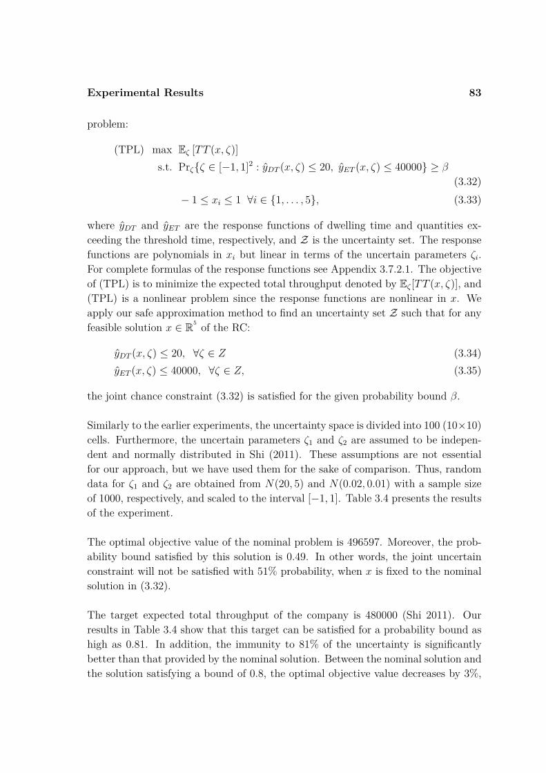
Experimental Results 83
problem:
(TPL) max Eζ [TT (x, ζ)]s.t. Prζζ ∈ [−1, 1]2 : yDT (x, ζ) ≤ 20, yET (x, ζ) ≤ 40000 ≥ β
(3.32)− 1 ≤ xi ≤ 1 ∀i ∈ 1, . . . , 5, (3.33)
where yDT and yET are the response functions of dwelling time and quantities ex-ceeding the threshold time, respectively, and Z is the uncertainty set. The responsefunctions are polynomials in xi but linear in terms of the uncertain parameters ζi.For complete formulas of the response functions see Appendix 3.7.2.1. The objectiveof (TPL) is to minimize the expected total throughput denoted by Eζ [TT (x, ζ)], and(TPL) is a nonlinear problem since the response functions are nonlinear in x. Weapply our safe approximation method to find an uncertainty set Z such that for anyfeasible solution x ∈ R5 of the RC:
yDT (x, ζ) ≤ 20, ∀ζ ∈ Z (3.34)yET (x, ζ) ≤ 40000, ∀ζ ∈ Z, (3.35)
the joint chance constraint (3.32) is satisfied for the given probability bound β.
Similarly to the earlier experiments, the uncertainty space is divided into 100 (10×10)cells. Furthermore, the uncertain parameters ζ1 and ζ2 are assumed to be indepen-dent and normally distributed in Shi (2011). These assumptions are not essentialfor our approach, but we have used them for the sake of comparison. Thus, randomdata for ζ1 and ζ2 are obtained from N(20, 5) and N(0.02, 0.01) with a sample sizeof 1000, respectively, and scaled to the interval [−1, 1]. Table 3.4 presents the resultsof the experiment.
The optimal objective value of the nominal problem is 496597. Moreover, the prob-ability bound satisfied by this solution is 0.49. In other words, the joint uncertainconstraint will not be satisfied with 51% probability, when x is fixed to the nominalsolution in (3.32).
The target expected total throughput of the company is 480000 (Shi 2011). Ourresults in Table 3.4 show that this target can be satisfied for a probability bound ashigh as 0.81. In addition, the immunity to 81% of the uncertainty is significantlybetter than that provided by the nominal solution. Between the nominal solution andthe solution satisfying a bound of 0.8, the optimal objective value decreases by 3%,

Experimental Results 84
Table 3.4 – Results for CDDC Example
β γ(S, α∗) Ω BBΩ |V | − |S| Obj.Nom. 0.49 0 0 50 4965970.6 0.62 0.1 0∗∗ 44 4910960.7 0.72 0.18 0.21 40 4865340.8 0.81 0.27 0.21 36 4815070.9 0.9 0.44 0.61 31 4728700.91 0.92 0.46 0.61 29 4719250.92 0.92 0.46 0.61 29 4719250.93 0.94 0.51 0.74 23 4693860.94 0.94 0.51 0.74 23 4693860.95 0.95 0.56 0.74 20 4671290.96 0.96 0.62 0.83 18 4645400.97 0.97 0.66 0.83 15 4628840.975 0.98 0.71 0.9 12 4608900.98 0.98 0.76 0.91 10 4589770.99 0.99 0.86 0.94 6 455381FRC 1 >1.41∗∗∗ 1 0 445172∗ α = 0.001, ∗∗ 2× 10⁻⁸ ≈ 0, ∗∗∗
√2 ≈ 1.41
while there is a 32% increase in the immunity to uncertainty. On the other hand, forprobability bounds above 0.9, we can no longer satisfy the target. For instance, ouroptimal solution can not satisfy 5% of 480000, when the prescribed probability is 0.99.
The trade-off between the probability guarantee and the optimal objective value isclear in the reported results. Using the solutions in Table 3.4, the decision maker canselect the best strategy for the new distribution system. This could involve accept-ing a small reduction from the expected target for the sake of a higher probabilityguarantee, or satisfying the target with a lower guarantee.
Dependent Data. Later in this example, we use the dependent data that is pre-sented in Table 3.15; see Appendix 3.8.4. The data is obtained using a bivariatenormal distribution by post-processing the “tail” cells that have less observations.The values in Table 3.15 correspond to the number of observations in the associatedcells and the sample size is 3033, hence the frequency of a cell can be calculated bydividing the number of observations in the associated cell to the sample size. Thetotal number of cells is again 100.

Experimental Results 85
Table 3.5 – Results for Dependent Data
β γ(S, α∗) Ω BBΩ |V | − |S| Obj.Nom. 0.36 0 0 50 4965970.6 0.62 0.24 0.06 37 4831610.7 0.71 0.45 0.26 30 4723970.8 0.81 0.51 0.36 23 4693870.9 0.90 0.71 0.52 12 4608900.91 0.91 0.75 0.53 11 4593540.92 0.93 0.81 0.57 8 4571430.93 0.94 0.86 0.57 6 4553820.94 0.95 0.99 0.74 3 4511260.95 0.95 1.04 0.8 1 4496030.96 1 1.09 0.81 0 4481390.97 1 1.09 0.81 0 4481390.98 1 1.09 0.81 0 4481390.99 1 1.09 0.81 0 448139FRC 1 >1.41∗∗ 1 0 445172∗ α = 0.001, ∗∗
√2 ≈ 1.41
According to the given data, we apply our safe approximation method to the CDDCproblem and the numerical results are reported in Table 3.5. The uncertainty setsthat are reported in Table 3.5 are larger than the ones provided in Table 3.4. This isbecause of three reasons: First is the data structure, e.g., extensive data locate on thecorners of the uncertainty region, namely, the top-left and the bottom-right cornersin Table 3.15. Second, the ρ value in constraint (3.8) increases, since the degrees offreedom increases. Note that the degrees of freedom is 99 for the dependent case;whereas it is 81 for the independent case. Third, the sample size of the dependentdata is smaller than that of the independent data. As a result, to satisfy the sameprobability guarantees we require larger uncertainty sets. Note that a larger uncer-tainty sets implies a conservative RC and this is why the optimal objective values inTable 3.5 are lower than the ones in Table 3.4. Nevertheless, we still have significantimprovements to the nominal solution. For instance, the solution satisfying a boundof 0.6 has 26% higher immunity to uncertainty than that of the nominal solutionand it is a considerable improvement for a 2.7% loss in the optimal objective value.For probability bounds that are higher than 0.95, the safe approximation methodfinds the same tight uncertainty set yielding the probability bound of one (using thediscretization and the center point assumption of the safe approximation method).

Experimental Results 86
Furthermore, the optimal objective value of the RC with BB1.09 is 0.6% higher thanthe worst-case optimal 445172 (FRC).
To conclude, it is clear that using the safe approximation method yields significantimprovements to the immunity to uncertainty, provided by the nominal solution, forrelatively small losses in terms of the optimal objective value.
3.4.3 Optimizing Color Picture TubeIn the manufacturing process of a standard television, the color picture tube is assem-bled to the other components using a manufacturing oven. The oven temperaturecauses thermal stresses on different points of the tube and if the temperature is toohigh, it will scrap the tube due to implosions. Figure 3.6 taken from Hertog andStehouwer (2002) gives an example of a temperature profile on a tube.
Figure 3.6 – Temperature Profile
To minimize the cost and hence the number of scraps, the manufacturer would like tomake an optimal temperature profile such that the temperatures are in the specifiedrange, the temperature differences between near locations are not too high and themaximal stress for the TV tube is minimal. Den Hertog and Stehouwer (2002)formulated the associated problem as follows:
min smax
s.t. ak + bTk x− smax ≤ 0 ∀k ∈ 1, . . . , K (3.36)−4Tmax ≤ Ax ≤ 4Tmax (3.37)l ≤ x ≤ u, (3.38)
where smax ∈ R is the maximal stress, ak + bTk x ∈ R is the stress at location k, i.e.,linear in x, and x ∈ Rn represents the vector of temperatures. The vectors l ∈ Rn

Experimental Results 87
and u ∈ Rn are the lower and upper bounds of the decision variables, respectively.The parameter 4Tmax ∈ Rd represents the maximal allowed temperature on d loca-tion combinations. A ∈ Rd×n coincides with the coefficients in the linear constraintsthat enforce the specified temperatures do not differ more than 4Tmax. There are 20temperature points on the TV tube and hence n = 20; see Figure 3.6. Furthermore,these temperatures result in 216 thermal stresses on different parts of the tube soK = 216. The response functions of the thermal stresses, ak + bTk x, are derived byusing FEM simulator and regression in Den Hertog and Stehouwer (2002). In thisexample, we use the same response functions, but the decision variable xi is replacedby xi(1 + ζj), where ζj is the multiplicative uncertain parameter, i.e., commonly re-ferred as the implementation error (e.g., ζj = 0.2 means 20% implementation errorin xi).
According to the proximity of the temperature points, we form the following sixsubgroups:
j 1 2 3 4 5 6T (j) 1 2,5,10 3,6,7,8 4,9,14 11,12,13 15,16,17,18,19,20
T (j) denotes the set of indices of the decision variable(s) that are assumed to beaffected by the same uncertain parameter ζj. This is a valid assumption since closerpoints in the TV tube have similar temperatures in practice. Eventually, using thesafe approximation method, our objective is to find the tightest uncertainty set Zfor the RC:
min smax
s.t. ak +6∑j=1
∑i∈T (j)
bikxi(1 + ζj)− smax ≤ 0 ∀k ∈ 1, . . . , K,∀ζ ∈ Z (3.39)
(3.37), (3.38),
such that the joint chance constraint:
Prζζ ∈ [−1, 1]6 : ak +
6∑j=1
∑i∈T (j)
bikxi(1 + ζj) ≤ smax, ∀k ∈ 1, . . . , K≥ β
(3.40)
is satisfied for any feasible RC solution (x, smax), where β is the given probabilitybound. The RC problem has 21 decision variables including smax, six primitive un-certain parameters, 216 linear uncertain constraints (i.e., given by constraint (3.39))and 56 linear constraints (i.e., given by constraints (3.37) and (3.38)).

Experimental Results 88
Data. The data for implementation errors are invented by us and the data range isdivided to five equal intervals. The frequencies of the associated intervals are shownin Table 3.16 and 3.17; see Appendix 3.8.4, we have the same frequencies in twodifferent data ranges that are: [-.1, .1] and [-.2, .2]. These ranges correspond to 10%and 20% implementation errors, respectively. In addition, we assume the uncertainparameters are independent and hence the frequency of a cell may be found by mul-tiplying the frequencies of the associated intervals for (ζ1, ζ2, ζ3, ζ4, ζ5, ζ6). The totalnumber of cells in the joint uncertainty space is 15625 (56).
The numerical results are shown in Table 3.6 and Table 3.7. In both tables, it is easy
Table 3.6 – TV Tube Example (10% Imp. Err.)
β γ(S, α∗) Ω |V | − |S| Obj.Nom 0∗∗ 0 15625 14.140.3 0.3 0.56 12642 14.40.35 0.35 0.6 11967 14.420.4 0.41 0.64 11245 14.440.45 0.46 0.68 10447 14.450.5 0.53 0.72 9547 14.470.6 0.63 0.78 8031 14.50.7 0.71 0.84 6753 14.520.75 0.76 0.88 5938 14.540.8 0.82 0.94 4772 14.560.85 0.85 0.98 4046 14.580.9 0.91 1.06 2833 14.610.92 0.93 1.1 2321 14.630.95 0.95 1.16 1648 14.650.96 0.97 1.2 1300 14.670.97 0.97 1.22 1140 14.680.98 0.98 1.28 736 14.70.99 0.99 1.34 455 14.73FRC 1 >2.45∗∗∗ 0 14.91∗ α = 0.001, ∗∗ 2×10⁻⁸ ≈ 0, ∗∗∗
√6 ≈ 2.45
to see that the nominal solution is not immune to the implementation errors. Tobe more precise, if the decision variables (x, smax) are fixed to the nominal solutionin the joint chance constraint (3.40), then the left-hand side probability is almostzero (i.e., 2 × 10⁻⁸). This means that the ζ values that are feasible for the joint

Experimental Results 89
constraint, are realized with almost zero probability. This is why implementing thenominal solution can be a risky decision in practice, but using the safe approximationmethod we can find significantly better solutions.
The numerical results in Table 3.6 show: Between the nominal solution and thesolution satisfying a bound of 0.3, the optimal objective value increases by 1.8%,while there is a 30% increase in the immunity to uncertainty. In addition, the solutionsatisfying a bound of 0.85 has an optimal objective value that is 3% higher than thatof the nominal solution. These are significant improvements in the immunity touncertainty for the losses in the optimal objective value.
Table 3.7 – TV Tube Example (20% Imp. Err.)
β γ(S, α∗) Ω |V | − |S| Obj.Nom. 0∗∗ 0 15625 14.140.3 0.31 0.56 12626 14.640.35 0.37 0.6 11857 14.670.4 0.43 0.64 11015 14.70.45 0.46 0.66 10593 14.720.5 0.53 0.7 9680 14.750.6 0.63 0.76 8078 14.80.7 0.71 0.82 6640 14.850.75 0.75 0.86 5906 14.870.8 0.82 0.92 4594 14.920.85 0.86 0.96 3776 14.950.9 0.9 1.02 2827 14.990.92 0.92 1.06 2286 15.020.95 0.95 1.14 1463 15.070.96 0.97 1.18 1114 15.10.97 0.97 1.2 950 15.110.98 0.98 1.24 676 15.130.99 0.99 1.3 372 15.17FRC 1 > 2.45∗∗∗ 0 15.44∗ α = 0.001, ∗∗ 2×10⁻⁸ ≈ 0, ∗∗∗
√6 ≈ 2.45
Note that when we increase the implementation errors from %10 to %20, then thevariance from the nominal case increases and we require larger tight uncertainty setsto satisfy the same probability bounds. This is why the number of cells removed fromthe full space of uncertainty is fewer when the implementation errors are higher; see

Conclusions 90
the fourth columns of Table 3.6 and 3.7. A larger tight uncertainty set implies amore restrictive RC and hence the optimal objective values shown in Table 3.7 areon average 2.2% higher than those provided in Table 3.6. The lowest difference be-tween two optimal objectives, i.e., 1.7%, is obtained at 0.3 probability bound, andthe highest, i.e., 2.9%, is obtained at 0.99, and there is a gradual increase in between.
3.5 ConclusionsIn this chapter, we have proposed new safe approximations for joint chance con-straints. Using historical data and goodness-of-fit statistics based on φ-divergence,we constructed the uncertainty sets that are used in safe approximations. The nu-merical results show that our approach yields tighter uncertainty sets, and thereforebetter objective values than the existing method, for the same probability guaran-tees, especially when the number of uncertain parameters is low. In addition, wedo not impose the assumptions that the uncertain parameters are independent orcertain moments are known. Last but not least, the new approach can also handlenonlinear inequalities.
It is important to observe that the computational performance of our approach ishighly dependent on the number of uncertain parameters. Furthermore, we mayrequire many data points, especially when the uncertain parameters are dependentand the number of uncertain parameters is high, and this data requirement may behard to manage in practice. In future research, we will investigate the improvementof our approach in such situations. The extension of our approach to simulationbased optimization and nonlinear problems will also be further analyzed in futureresearch.

Derivation of Robust Counterpart 91
APPENDICES
3.6 Derivation of Robust CounterpartLet Z = ζ : Psζ + ps ∈ Ks, s = (1, . . . , S) where Ks denotes a closed convexpointed cone with a non-empty interior. The semi-infinite representation:
(a0 +∑i=1
ζiai)Tx ≤ b, ∀ζ ∈ Z
is equivalent to the following RC:
maxζ∈Z
(a0 +
∑i=1
ζiai)Tx
≤ b. (3.41)
Using the Conic Duality theorem, (3.41) is equivalent to
minys∈Ks
∗ :s∈1,...,S
S∑s=1
pTs ys + (a0)Tx
≤ b
S∑s=1
(P Ts y
s)j = −(a`)Tx ∀j ∈ 1, . . . , `,(3.42)
where Ks∗ denotes the dual cone of Ks. For the detailed derivation of (3.42), see
Theorem 1.3.4 and Corollary 1.3.6 of Ben-Tal et al. (2009). Then the minimizationin (3.42) is removed—as it is often done in RO—and we have the following equivalentsystem of conic inequalities:
S∑s=1
pTs ys + (a0)Tx ≤ b
S∑s=1
(P Ts y
s)j = −(a`)Tx ∀j ∈ 1, . . . , `
ys ∈ Ks
∗ ∀s ∈ 1, . . . , S.
(3.43)
The conic representation of the uncertainty set BBΩ(c) is equivalent to
Z = ζ : P1ζ + p1 ∈ K1, P2ζ + p2 ∈ K2
where
• P1ζ ≡ [ζ; 0], p1 ≡ [01×`; 1] and K1 := (e, t) ∈ R` ]× R : ||e||∞ ≤ t
• P2ζ ≡ [ζ; 0], p2 ≡ [−c; Ω] and K2 := (e, t) ∈ R` × R : ||e||2 ≤ t.

Data and Additional Results 92
Then using (3.43), the RC for BBΩ(c) is equivalent to
τ1 − wT c+ Ωτ2 + (a0)Tx ≤ b
(z + w)` = −(aj)Tx, j = (1, . . . , `)||z||1 ≤ τ1 (K1
∗ := (z, τ1) ∈ R` × R : ||z||1 ≤ τ1)||w||2 ≤ τ2 (K2
∗ := (w, τ2) ∈ R` × R : ||w||2 ≤ τ2),
(3.44)
where y1 = [z; τ1] ∈ K1∗ and y2 = [w; τ2] ∈ K2
∗ . Consequently, (3.44) is equivalent to
∑j=1|zj|+ Ω
√√√√√∑j=1
w2j − wT c ≤ b− [a0]Tx,
zj + wj = −(aj)Tx, ∀j ∈ 1, ..., ` .
(3.45)
3.7 Data and Additional Results3.7.1 Extra Results for Example 4.1
Table 3.8 – Kullback-Leibler Distance
β γ(S, α∗) Ω BBΩ |V | − |S| Obj. Ωacc Objacc. %Improv.Nom. 0.5 0 0 45 10 - - -0.60 0.69 0.29 0.03 28 8.30 1.35 5.11 620.70 0.78 0.43 0.22 21 7.67 >1.41 5 53.40.80 0.86 0.57 0.35 15 7.13 >1.41 5 42.50.90 0.92 0.71 0.64 10 6.66 >1.41 5 33.20.91 0.92 0.71 0.64 10 6.66 >1.41 5 33.20.92 0.96 0.85 0.72 6 6.25 >1.41 5 24.90.93 0.96 0.85 0.72 6 6.25 >1.41 5 24.90.94 0.96 0.85 0.72 6 6.25 >1.41 5 24.90.95 0.96 0.85 0.72 6 6.25 >1.41 5 24.90.96 0.98 0.99 0.89 3 5.88 >1.41 5 17.60.97 0.98 0.99 0.89 3 5.88 >1.41 5 17.60.98 0.98 0.99 0.89 3 5.88 >1.41 5 17.60.98 0.99 1.14 0.95 1 5.54 >1.41 5 10.70.99 1 1.28 0.98 0 5 >1.41 5 0
1 - - - 5 - - -∗ α=0.001

Data and Additional Results 93
Table 3.9 – Hellinger Distance
β γ(S, α∗) Ω BBΩ |V | − |S| Obj. Ωacc Objacc. %Improv.Nom. 0.5 0 0 45 10 - - -0.60 0.66 0.29 0.03 28 8.30 1.35 5.11 620.70 0.75 0.43 0.22 21 7.67 >1.41 5 53.40.80 0.83 0.57 0.35 15 7.13 >1.41 5 42.50.90 0.94 0.85 0.64 6 6.25 >1.41 5 24.90.91 0.94 0.85 0.64 6 6.25 >1.41 5 24.90.92 0.94 0.85 0.64 6 6.25 >1.41 5 24.90.93 0.94 0.85 0.64 6 6.25 >1.41 5 24.90.94 0.96 0.99 0.89 3 5.88 >1.41 5 17.60.95 0.96 0.99 0.89 3 5.88 >1.41 5 17.60.96 0.96 0.99 0.89 3 5.88 >1.41 5 17.60.97 0.98 1.14 0.95 1 5.54 >1.41 5 10.70.98 0.98 1.14 0.95 1 5.54 >1.41 5 10.70.99 1 1.27 0.98 0 5 >1.41 5 0
1 - - - - 5 - - -∗ α=0.001
3.7.2 Example 4.33.7.2.1 Response Functions
Eζ [TT (x, ζ)] =− 479700− 39819.17 ∗ x(1)− 20253.25 ∗ x(2) + 312.12 ∗ x(3)− 7339.86 ∗ x(4)− 339.78 ∗ x(5)−7895.49 ∗ x(1) ∗ x(2)− 121.06 ∗ x(1) ∗ x(3)− 33.75 ∗ x(1) ∗ x(4) + 21.24 ∗ x(1) ∗ x(5)−7.36 ∗ x(2) ∗ x(3) + 649.55 ∗ x(2) ∗ x(4) + 1136.31 ∗ x(2) ∗ x(5) + 788.4 ∗ x(3) ∗ x(4)+407.64 ∗ x(3) ∗ x(5)− 1101.55 ∗ x(4) ∗ x(5) + 34063.49 ∗ x(1)2 + 17810.89 ∗ x(2)2+108.13 ∗ x(3)2 + 10333.23 ∗ x(4)2 − 1107.72 ∗ x(5)2.
yDT (x, ζ) =− 8.57 + 1.2 ∗ x(1) + 2.04 ∗ x(2)− 0.17 ∗ x(3) + 0.78 ∗ x(4) + 3.30 ∗ x(5)− 0.44 ∗ x(1) ∗ x(2)+0.29 ∗ x(1) ∗ x(3)− 0.26 ∗ x(1) ∗ x(4) + 0.33 ∗ x(1) ∗ x(5) + 0.21 ∗ x(2) ∗ x(3)− 0.45 ∗ x(2) ∗ x(4)+0.55 ∗ x(2) ∗ x(5)− 0.061 ∗ x(3) ∗ x(4) + 0.062 ∗ x(3) ∗ x(5) + 0.35 ∗ x(4) ∗ x(5)− 0.63 ∗ x(1)2−1.27 ∗ x(2)2 + 0.19 ∗ x(3)2 − 0.25 ∗ x(4)2 − 0.11 ∗ x(5)2+7.11 + 0.78 ∗ x(1) + 1.63 ∗ x(2)− 0.081 ∗ x(3) + 0.57 ∗ x(4) + 2.72 ∗ x(5) ∗ ζ1+3.21 + 0.46 ∗ x(1) + 0.49 ∗ x(2)− 0.073 ∗ x(3) + 0.16 ∗ x(4) + 1.17 ∗ x(5) ∗ ζ2 ≤ 0.
yET (x, ζ) =− 7517.8 + 10256.36 ∗ x(1) + 13753.61 ∗ x(2)− 300.42 ∗ x(3) + 4379.24 ∗ x(4) + 52.43 ∗ x(5)+5415.96 ∗ x(1) ∗ x(2) + 437.38 ∗ x(1) ∗ x(3) + 214.75 ∗ x(1) ∗ x(4) + 597.11 ∗ x(1) ∗ x(5)−97.79 ∗ x(2) ∗ x(3)− 1618.36 ∗ x(2) ∗ x(4)− 724.67 ∗ x(2) ∗ x(5)− 1639.28 ∗ x(3) ∗ x(4)−1243.25 ∗ x(3) ∗ x(5) + 1728.59 ∗ x(4) ∗ x(5)−1118.43 ∗ x(1)2 − 1072.35 ∗ x(2)2 + 226.71 ∗ x(3)2 − 372.2 ∗ x(4)2 + 148.92 ∗ x(5)2+36087.44 + 13066.74 ∗ x(1) + 17605.17 ∗ x(2)− 739.11 ∗ x(3) + 5944.33 ∗ x(4) + 446.33 ∗ x(5) ∗ ζ1+−10868− 3824.22 ∗ x(1)− 5975.83 ∗ x(2) + 209.48 ∗ x(3)− 2506.4 ∗ x(4)− 579.61 ∗ x(5) ∗ ζ2 ≤ 0.

Additional Experiments 94
3.8 Additional Experiments3.8.1 Comparison with Randomized ApproachIn this experiment, we apply the randomized approach that is proposed by Calafioreand Campi (2005) to the illustrative experiment shown in §3.4.1. The objective is tocompare these results to that of the safe approximation method reported in Table 3.3.
Calafiore and Campi (2005) propose a randomized algorithm for uncertain convexoptimization problems. The algorithm is as follows: For an uncertain constraint[f(x, ζ) ≤ 0] at hand, they randomly extract N realizations of the uncertain param-eter (ζ) in an independent fashion using the known probability distribution (P) of ζ.Note that each extraction (ζ) coincides with a discrete constraint [f(x, ζ) ≤ 0]. Then,instead of the exact uncertain problem, they solve the one with randomly extractedN constraints. Eventually, the optimal solution of the randomized approach satisfiesthe following probability bound that is proved by Campi and Garatti (2008):
PrV (x∗N ) > ε ≤d−1∑i=0
(Ni
)εi(1− ε)N−i︸ ︷︷ ︸
BεNd
, (3.46)
where Bε
Nd corresponds to the associated probability bound, V (x) denotes the vio-lation probability for a given solution x ∈ Rn , ε is the given violation probabilitybound that is “generally” close to zero and x∗N ∈ Rn coincides with the optimalsolution of the convex optimization problem with randomly selected N constraints.For a detailed overview of the randomized approach, we refer to Calafiore and Campi(2005), Calafiore (2006) and Campi and Garatti (2008). If we relate (3.46) to ournotation:
[Pr
Prζ∼Pζ : f(x, ζ) ≤ 0 ≥ β≥ 1− α
], then the probability bound β
of the chance constraint coincides with 1 − ε and the confidence level 1 − α corre-sponds to 1 − Bε
Nd (i.e., Bε
Nd = α). This means we should find the closest N valuethat satisfies Bε
Nd∼= α (see Table 3.10 for the values of N when d = 2).
Notice that the probability distribution P is unknown in the safe approximationmethod proposed in this chapter. However, the disadvantage of the randomized ap-proach is that P has to be known since constraints are extracted according to a knownP. Therefore, we assume that the empirical estimates, i.e., q in our notation, denotethe required probability distribution P for the randomized approach. As a remarkwe have 100 cells in the uncertainty space so that each independent draw is donefrom 100 constraints. Notice that N can be larger than 100 for given β and α, and

Additional Experiments 95
Table 3.10 – Randomized versus Safe Approximation
(α = 0.001) Obj. Val.β N ∗ RA∗∗ SA
0.6 19 6.15 9.040.7 27 6.12 8.290.8 42 5.8 7.120.9 88 5.56 6.650.91 98 5.47 6.650.92 111 5.45 6.650.93 127 5.48 6.240.94 149 5.42 6.240.95 180 5.34 6.240.96 226 5.32 5.880.97 303 5.21 5.880.98 457 5.16 5.530.99 919 5 5∗ d = 2, ∗∗ Avg. of 20 rep.
due to randomization a constraint can be selected more than one time. Finally, fordifferent probability bounds we compare the optimal objective value of the random-ized approach to that of the safe approximation method proposed in this chapter.The numerical results are shown in Table 3.10, where the last column (SA), takenfrom the results of Experiment 3.4.1, is the optimal objective value of the safe ap-proximation method. Note that for the randomized approach we report the averageobjective value of 20 replications in the third column of Table 3.10, i.e., denoted byRA. This is done to have a fair comparison between the two approaches.
The numerical results in Table 3.10 show that the safe approximation method per-forms better than the randomized approach. This is a logical outcome, since the safeapproximation method is more objective oriented and takes into account the optimalsolution, to construct the uncertainty set, at each iteration of the algorithm. On theother hand, the randomized approach does not consider the objective value whileextracting constraints. Secondly, the numerical results also show that the differencebetween the two approaches decreases as the probability bound β increases. This isanother expected result, since for probability bounds close to 1 the uncertainty sethas to be close to the full space of the uncertainty, which means that there is nodifference between the two approaches in this case.

Additional Experiments 96
3.8.2 Comparison with One-by-One ApproachThe objective of this section is to compare the optimal objective values of the one-by-one approach (that is addressed in §3.3.2) to that of the safe approximation methodproposed in the chapter. The numerical example is selected as the illustrative ex-periment in §3.4.1 (i.e., the results of the safe approximation method for the givenprobability bounds are taken from Table 3.3). The numerical results are presentedin the following table.
Table 3.11 – One-by-One versus Safe Approximation
βObj. Val.
1-by-1 SA0.92 6.65 6.650.93 6.25 6.240.94 6.25 6.240.95 6.25 6.240.96 5.88 5.880.97 5.88 5.880.98 5.55 5.530.99 5 5α = 0.001
Note that the one-by-one approach provides the “exact” optimal solution for a givenprobability bound with a confidence level of 1−α, but it requires many more iterationscompared to our method as the probability bound gets lower. The numerical resultsreveal that the safe approximation method yields objective values that are very close(or the same) to the one-by-one approach.
3.8.3 Multi-Period Work Scheduling ProblemIn this experiment, we solve a modified version of multi-period work scheduling(MWS) problem. MWS is a linear optimization problem used to schedule employeesfor a multi-period time horizon where the demand changes over time.
Computer Service Store. CLS is a computer service store that requires the fol-lowing skilled-repair times in the next five months: 3000, 3500, 4000, 4500, and 5500.The repair work is done by skilled technicians and these technicians can each workup to 160 hours per month. Furthermore, the technicians may train apprentices tomeet future demand. It takes an average of 50 hours to train an apprentice, and

Additional Experiments 97
new technicians start serving CLS in the month following their training session. Inaddition, the training sessions have 100% efficiency, so an apprentice always becomesa technician at the end of the training period. The hiring of technicians is done onlyin the first period and the start-up cost of hiring a technician is $8000. In addition,each technician is paid $2000 and each apprentice costs $1000 per month. On theother hand, 5% of the technicians quit at the end of each month. Finally, the objec-tive of CLS is to minimize the total labor cost incurred to meet the demand in thenext five months. The mathematical model of this problem is presented below:
(NMWS) min5∑i=1
1000xi +5∑i=1
2000yi + 8000y1
s.t. 160yi − 50xi ≥ di i ∈ 1, . . . , 5 (3.47)0.95yi + xi = yi+1 i ∈ 1, . . . , 4 (3.48)xi, yi ≥ 0 i ∈ 1, . . . , 5 , (3.49)
where yi represents the number of technicians, xi corresponds to the number of ap-prentices in training, and di is the repair time demanded in period i ∈ 1, . . . , 5. Inpractice, the average working and training hours usually deviate from the estimatedvalues because of overtime, illness, vacations, and other factors. We have historicaldata for 120 months giving the average working and training hours spent per techni-cian each month. These data are used in Table 3.12 to derive the frequencies. Note
Table 3.12 – Frequencies for Working (W.H.) and Training (T.H.) Hours
ζ1, ζ2 [-1 -0.8] [-0.8 -0.6] [-0.6 -0.4] [-0.4 -0.2] [-0.2 0] [0 0.2] [0.2 0.4] [0.4 0.6] [0.6 0.8] [0.8 1]W.H. [120 128] [128 136] [136 144] [144 152] [152 160] [160 168] [168 176] [176 184] [184 192] [192 200]
freq.(ζ1) 0.02 0.04 0.1 0.1 0.2 0.3 0.1 0.1 0.02 0.02T.H. [30 34] [34 38] [38 42] [42 46] [46 50] [50 54] [54 58] [58 62] [62 66] [66 70]
freq.(ζ2) 0.015 0.07 0.1 0.15 0.15 0.17 0.15 0.11 0.07 0.015
that the working hours range from 120 to 200, so the mean is 160 and the half-lengthof the data range is 40. Similarly, for the training hours the mean is 50 and thehalf-length of the data range is 20. Using this information from the historical data,we introduce uncertainty to constraint (3.47) as follows:
min5∑i=1
1000xi +5∑i=1
2000yi + 8000y1
s.t. Prζζ ∈ [−1, 1]2 : (160 + 40ζ1) yi − (50 + 20ζ2)xi ≥ di, ∀i ∈ 1, . . . , 5 ≥ β
(3.50)(3.48), (3.49),
where ζ1 ∈ [−1, 1] and ζ2 ∈ [−1, 1] are the uncertain parameters, and β is theprescribed probability bound. The frequencies of the working and training hours are

Additional Experiments 98
scaled into the frequencies of ζ1 and ζ2 in Table 3.12. Furthermore, the uncertainparameters are independent; therefore, the joint frequencies can be derived similarlyto the first experiment. The joint uncertainty region is again divided into 100 (10×10) cells. Eventually, using our safe approximation method, we find the tightestuncertainty set Z such that for any feasible solution (x, y) of the RC:
(160 + 40ζ1) yi − (50 + 20ζ2)xi ≥ di,∀i ∈ 1, . . . , 5 , ∀ζ ∈ Z, (3.51)
the joint chance constraint (3.50) is satisfied for the given probability bound β. Inthis experiment we use the extension in §3.3.3.1, i.e., the safe approximation of thejoint chance constraint. The results are reported in Table 3.13.
Table 3.13 – Results for CLS Example
β γ(S, α∗) Ω BBΩ |V | − |S| Obj.Nom. 0.49 0 0 50 4481050.6 0.63 0.12 0∗∗ 44 4626910.65 0.66 0.14 0∗∗ 43 4652140.7 0.75 0.3 0.12 35 4864340.75 0.77 0.32 0.12 34 4892220.8 0.8 0.38 0.33 31 4977820.85 0.86 0.5 0.38 25 5158300.9 0.9 0.56 0.55 22 5253510.91 0.91 0.58 0.55 21 5286030.92 0.94 0.7 0.66 15 5489880.93 0.94 0.7 0.66 15 5489870.94 0.94 0.72 0.8 14 5525380.95 0.95 0.74 0.8 13 5561340.96 0.96 0.78 0.85 11 5634680.97 0.98 0.9 0.9 5 5866720.98 0.98 0.94 0.93 3 5948340.99 0.99 0.98 0.95 1 603225FRC 1 >1.41∗∗∗ 1 0 621356∗ α = 0.001, ∗∗ 1.9×10⁻⁸ ≈ 0, ∗∗∗
√2 ≈ 1.41
The meanings of the columns in Table 3.13 are the same as for the first experiment.Note that the optimal objective values for the nominal problem (NMWS) and therobust counterpart for the full space of uncertainty (FRC) are 448105 and 621356,respectively (see the first and last row of Table 3.13). The results show that when

Additional Experiments 99
the probability bound is as low as 0.6, the optimal objective value calculated by thealgorithm is 3% higher than that of the nominal solution. Moreover, with respect tothe nominal solution, we see a 14% increase in the immunity to uncertainty in con-straint (3.50), which is a considerable improvement for a 3% sacrifice in terms of theobjective value. For the higher probability bounds of 0.92 and 0.94, the improvementin the optimal objective value of FRC is 12% and 11%, respectively. Furthermore,for the probability bound of 0.98, the algorithm improves the objective value of FRCby 4% and the solution is robust to at least 98.3% of the uncertainty. It is clearthat when the probability bound β increases, we remove fewer cells from the initialuncertainty region and the radius Ω of BBΩ gets larger. Ultimately, the decisionmaker must make the decision by looking at the results in Table 3.13 and choosingthe best option for CLS.
Later in this example, we consider the extension in §3.3.3.3, i.e., using the box insteadof the ellipsoid as the starting uncertainty set of our algorithm. Note that we applythis extension to the same problem. In addition, we test the new approach for thesame data set and when the inputs of the algorithm such as the number of cells andstep size ω are held constant. The numerical results are presented in Table 3.14. Thesymbol (∗) denotes an instance where using the box yields a better optimal objectivevalue than using the ellipsoid for a given probability bound β.

Additional Experiments 100
Table 3.14 – Results for CLS Example (Box)
β γ(S, α∗) Ω |V | − |S| Obj.Nom. 0.49 0 50 4481050.6 0.63 0.1 44 461039(∗)0.65 0.66 0.12 43 463715(∗)0.7 0.78 0.3 33 4892360.75 0.78 0.3 33 4892360.8 0.80 0.34 31 495286(∗)0.85 0.90 0.5 22 5210220.9 0.90 0.5 22 5210220.91 0.91 0.52 21 524423(∗)0.92 0.96 0.7 11 5571070.93 0.96 0.7 11 5571070.94 0.96 0.7 11 5571070.95 0.96 0.7 11 5571070.96 0.96 0.7 11 557107(∗)0.97 1 0.9 0 5984020.98 1 0.9 0 5984020.99 1 0.9 0 598402(∗)FRC 1 >1.41∗∗ 0 621356∗ α = 0.001, ∗∗
√2 ≈ 1.41
The numerical results reveal that using the box or the ellipsoid as the starting uncer-tainty set yields similar optimal objective values, e.g, the highest difference betweenoptimal objective values of two approaches is around 1%. Nevertheless, using theellipsoid is more flexible in finding the final tight uncertainty sets for the CLS prob-lem. For instance, if the probability bound is in between 0.92 and 0.96 or higher than0.96, then the safe approximation method using the box finds only one uncertaintyset for each of the cases; whereas, the results in Table 3.13 show that the safe ap-proximation method using the ellipsoid finds a unique tight uncertainty set for eachof the probability bounds (except 0.92 and 0.93).
3.8.4 Dependent Data Set and Data Set of Example 4.4

Additional Experiments 101
Table 3.15 – Dependent Data used in Example 4.3
ζ2
Cells 1 2 3 4 5 6 7 8 9 10
ζ1
1 66 30 27 23 9 5 5 5 5 52 53 35 38 23 8 13 5 5 5 53 42 28 53 35 44 28 17 6 5 54 32 35 44 79 81 49 26 28 9 55 28 23 53 85 86 70 69 31 14 136 15 15 41 46 83 102 83 67 23 207 5 6 12 36 46 75 73 51 38 308 5 8 5 14 30 49 65 43 38 429 5 5 5 7 15 20 25 34 28 5610 5 5 5 5 5 12 15 28 15 79
(∗) N = 3033
Table 3.16 – Data Set 1 (10% Imp. Err.)
[-.1 -.06] [-.06 -.02] [-.02 .02] [.02 .06] [.06 .1]ζ1 0.1 0.21 0.29 0.22 0.18ζ2 0.09 0.18 0.38 0.23 0.12ζ3 0.13 0.23 0.3 0.17 0.17ζ4 0.11 0.22 0.31 0.24 0.12ζ5 0.09 0.2 0.28 0.23 0.2ζ6 0.17 0.22 0.23 0.2 0.18(∗) Nj = 100 ∀j ∈ 1, . . . , 6
Table 3.17 – Data Set 2 (20% Imp. Err.)
[-.2 -.12] [-.12 -.04] [-.04 .04] [.04 .12] [.12 .2]ζ1 0.1 0.21 0.29 0.22 0.18ζ2 0.09 0.18 0.38 0.23 0.12ζ3 0.13 0.23 0.3 0.17 0.17ζ4 0.11 0.22 0.31 0.24 0.12ζ5 0.09 0.2 0.28 0.23 0.2ζ6 0.17 0.22 0.23 0.2 0.18(∗) Nj = 100 ∀j ∈ 1, . . . , 6

Bibliography
Bemis, C., X. Hu, W. Lin, S. Moazeni, L. Wang, T. Wang, J. Zhang. 2009. Robustportfolio optimization using a simple factor model. IMA Preprint Series No. 2284,University of Minnesota, Minneapolis, MN.
Birge, J. R., J. R. B. Wets. 1986. Designing approximation schemes for stochasticoptimization problems, in particular for stochastic programs with recourse. Math.Programming Stud. 27 54–102.
Ben-Tal, A., A. Nemirovski. 2000. Robust solutions of linear programming problemscontaminated with uncertain data. Math. Programming 88(3) 411–424.
Ben-Tal, A., A. Nemirovski. 2002. Robust optimization: methodology and applica-tions. Math. Programming 92(3) 453–480.
Ben-Tal, A., A. Nemirovski. 2009. On safe tractable approximations of chance-constrained linear matrix inequalities. Math. Oper. Res. 34(1) 1–25.
Ben-Tal, A., D. den Hertog, J.-P. Vial. 2012. Deriving robust counterparts of nonlin-ear uncertain inequalities. CentER Discussion Paper No. 2012-053, Tilburg Uni-versity, Tilburg, The Netherlands.
Ben-Tal, A., L. El Ghaoui, A. Nemirovski. 2009. Robust Optimization. PrincetonPress, Princeton, NJ.
Ben-Tal, A., D. den Hertog, A. De Waegenaere, B. Melenberg, G. Rennen. 2012.Robust optimization with uncertainty regions based on φ-divergence. CentER Dis-cussion Paper No. 2011-061, Tilburg University, Tilburg, The Netherlands. Man-agement Sci. Forthcoming.
Burkauskas, A. 1986. On the convexity problem of probabilistic constraint stochasticprogramming problems. Alkal. Matema. Lapok 12 77–90.
Calafiore, G. C. 2007. Ambiguous risk measures and optimal robust portfolios. SIAMJ. Optim. 18(3) 853–877.
Calafiore, G. C., M. C. Campi. 2005. Uncertain convex programs: randomized solu-tions and confidence levels. Math. Programming 102 25–46.
Campi, M., S. Garatti. 2008. The exact feasibility of randomized solutions of robustconvex programs. SIAM J. Optim. 19(3) 1211–1230.
Charnes, A., W. W. Cooper. 1959. Chance-constrained programming. Management

BIBLIOGRAPHY 103
Sci. 6(1) 73–79.Charnes, A., W. W. Cooper, G. H. Symonds. 1958. Cost horizons and certainty
equivalents: an approach to stochastic programming of heating oil. ManagementSci. 4(3) 235–263.
Chen, X., M. Sim, P. Sun. 2007. A robust optimization perspective on stochasticprogramming. Oper. Res. 55(6) 1058–1107.
Chen, W., M. Sim, J. Sun, C. P. Teo. 2010. From CVaR to uncertainty set: implica-tions in joint chance-constrained optimization. Oper. Res. 58(2) 470–485.
Den Hertog, D., P. Stehouwer. 2002. Optimizing color picture tubes by high-costnonlinear programming. Eur. J. Oper. Res. 140(2) 197–211.
Dupacova, J. 1987. The minimax approach to stochastic programming and illustra-tive application. Stochastics 20 73–88.
Dupacova, J. 2001. Encyclopedia of Optimization. Stochastic Programming: minimaxapproach. Kluwer Academic Publishers, Dordrecht, The Netherlands.
Epstein, L. G., M. Schneider. 2003. Recursive multiple-priors. J. Econom. Theory113(1) 1–31.
Epstein, L. G., M. Schneider. 2007. Learning under ambiguity. Rev. Econom. Stud.74(4) 1275–1303.
Erdogan, E., G. Iyengar. 2006. Ambiguous chance constrained problems and robustoptimization. Math. Programming 107(1–2) 37–61.
Fama, E. F., K. R. French. 1993. Common risk factors in the returns on stocks andbonds. J. Financial Economics 33(1) 3–56.
Gilboa, A. L., D. Schmeidler. 1989. Maxmin expected utility with non-unique prior.J. Mathematical Econom. 18(2) 141–153.
Hansen, L. P., T. J. Sargent. 2001. Robust control and model uncertainty. AmericanEconom. Rev. 91 60–66.
Henrion, R., C. Strugarek. 2008. Convexity of chance constraints with independentrandom variables. Computational Optim. Appl. 41 263–276.
Jager, L., J. A. Weller. 2007. Goodness-of-fit tests via phi-divergences. Ann. Statist.35 2018–2053.
Klabjan, D., D. Simchi-Levi, M. Song. 2007. Robust stochastic lot-sizing by meansof histograms. Technical report, MIT, Boston, MA.
Miller, B. L., H. M. Wagner. 1965. Chance constrained programming with jointconstraints. Oper. Res. 13(6) 930–945.
Myers, R. H., D. C. Montgomery. 1995. Response Surface Methodology: Process andProduct in Optimization Using Designed Experiments. John Wiley & Sons Inc.,New York, NY.

BIBLIOGRAPHY 104
Nemirovski, A., A. Shapiro. 2006. Convex approximations of chance constrained pro-grams. SIAM J. Optim. 17(4) 969–996.
Nemirovski, A., A. Shapiro. 2007. Convex approximations of chance constrained pro-grams. SIAM J. Optim. 17(4) 969–996.
Pardo, L. 2006. Statistical Inference Based on Divergence Measures. Chapman &Hall/CRC, Boca Raton, FL.
Prekopa, A. 1970. Efficient robust optimization of metal forming processes using asequential metamodel based strategy. In Proceedings of the Princeton Symposiumon Mathematical Programming, Princeton University Press, Princeton, NJ. 113–138.
Prekopa, A. 1973. On logarithmic concave measures and functions. Acta ScientiarumMathematicarum 34 335–343.
Prekopa, A. 1974. Programming under probabilistic constraints with a random tech-nology matrix. Mathematische Operationsforschung und Statistik 5 109–116.
Prekopa, A. 1995. Stochastic Programming. Kluwer Academic Publishers, Dordrecht,The Netherlands.
Shapiro, A., S. Ahmed. 2004. On a class of minimax stochastic programs. SIAM J.Optim. 14(4) 1237–1252.
Shapiro, A., A. J. Kleywegt. 2002. Minimax analysis of stochastic problems. Optim.Methods and Software 17 523–542.
Shi, W. 2011. Design of pre-enhanced cross-docking distribution center under supplyuncertainty: RSM robust optimization method. Working Paper, HUST, China.
Wiebenga, J. H., G. Klaseboer, A. H. van den Boogaard. Efficient robust optimizationof metal forming processes using a sequential metamodel based strategy. 2011.8th International Conference and Workshop on Numerical Simulation of 3D SheetMetal Forming Processes, August 2011, Korean Society for Technology of Plasticity,Numisheet 2011. 978–985.
Van de Panne, C., W. Popp. 1963. Minimum-cost cattle feed under probabilisticprotein constraints. Management Sci. 9(3) 405–430.
Zackova, J. 1966. On minimax solutions of stochastic linear programs. Cas. Pest.Mat.. 423–430.
Zymler S., D. Kuhn, B. Rustem. 2012. Distributionally robust joint chance con-straints with second-order moment information. Working Paper. Math. Program-ming Forthcoming.

CHAPTER 4
Adjustable Robust Optimization UsingMetamodels
4.1 IntroductionIn this chapter, we present a methodology that is a novel combination of robust op-timization (RO) and simulation-based robust parameter design (RPD). We mentionthe major contributions of our research at the end of this section, but before that weextensively describe the fields of RO and simulation-based RPD.
To begin with, the goal of many experiments is to estimate the best solution for agiven practical problem. Such experiments may be conducted with a physical system(e.g., an airplane model in a wind tunnel) or a mathematical model of a physicalsystem (e.g., a computerized simulation model of an airplane or an inventory man-agement system). These experiments produce data on the outputs or responses forthe given inputs or factors. Output may be univariate (a single or scalar response) ormultivariate (multiple responses or a vector with responses). The number of inputsmay range from a single input to ‘many’ inputs (e.g., thousands of inputs), but wefocus on practical problems with no more than (say) twenty inputs.
Taguchi (1987)—for an update see Myers et al. (2009, pp. 483–485)—distinguishesbetween the following two types of inputs: (i) Controllable or decision factors (say)dj (j = 1, . . . , k), collected in the k-dimensional vector d = (d1, . . . , dk)
T . (ii) En-vironmental or noise factors (say) eg (g = 1, . . . , c), collected in the c-dimensionalvector e = (e1, . . . , ec)
T . By definition, the first type of inputs is under the control ofthe users; e.g., in an inventory system, management controls the order quantity. Thesecond type of inputs is not controlled by the users; e.g., demand in an inventorysystem. Taguchi emphasizes that the noise factors create variability in the outputs.Consequently, the combination of decision factors that (say) maximizes the expectedunivariate output may cause the variance of that output to be much larger than a

Introduction 106
combination that ‘nearly’ maximizes the mean output; i.e., a little sacrifice in ex-pected output may save a lot of problems caused by the variability in the output (oras the French proverb states: “the best is the enemy of the good”).
Taguchian RPD has been criticized by statisticians; see the panel discussion reportedin Nair et al. (1992). Their main critique concerns the statistical design and analysisin the Taguchian approach; for details we refer to Taguchi (1987) and Myers et al.(2009, pp. 483–495). An alternative RPD approach is given by Myers et al. (2009,pp. 502–506). Like Myers et al. do, we expose our methodology using the following‘incomplete’ second-order polynomial regression metamodel:
y(e,d) = β0 + βTd + dTBd + γT e + dT∆e + ε (4.1)
that approximates the unknown input/output (I/O) function (say) w = g(e,d) fora single output w of the system, where y denotes the output of the regression meta-model of the simulation model with output w; β0 the intercept; β = (β1, . . . , βk)
T thefirst-order effects of the decision variables d; B the k×k symmetric matrix of second-order effects of d with on the main diagonal the ‘purely quadratic’ effects βj;j and offthis diagonal half the interactions between pairs of decision factors βj;j′/2 (j 6= j′);γ = (γ1, . . . , γc)
T the first-order effects of the environmental factors e; ∆ = (δj;g) thek×c pairwise (two-factor) interactions between d and e; ε the residual with E(ε) = 0if this model has no ‘lack of fit’ (so it is a valid or adequate approximation of g(e,d))and with constant variance σ2
ε .
Myers et al. (2009) assume experiments with real systems; whereas we assume ex-periments with simulation models of real systems. These simulation models may beeither deterministic (especially in engineering) or random (stochastic, possibly withdiscrete events). Deterministic simulation models have noise if a parameter or inputvariable has a fixed but unknown value; this is called subjective or epistemic uncer-tainty; see Iman and Helton (2006). Random simulation models also have objective,aleatory or inherent uncertainty; again see Iman and Helton. We focus on randomsimulation, but shall also discuss deterministic simulation. Simulation analysts usedifferent names for metamodels, such as response surfaces, surrogates, and emula-tors; see the many references in Kleijnen (2008, p. 8). There are different types ofmetamodels, but the most popular types are low-order polynomials such as (4.1) andKriging (Gaussian process) models. These polynomials are nonlinear in the inputs(e,d) but linear in the regression parameters (β0, . . . , δk;c) so the analysis may useclassic linear regression models estimated using the least squares (LS) criterion; seeKleijnen (2008, pp. 15–72) and Myers et al. (2009, pp. 13–71). Kriging models aremore flexible so they can accurately approximate the true I/O function over bigger

Introduction 107
experimental areas; see Kleijnen (2008, pp. 139–156). It is important to point outthat methods that shall be proposed in this chapter are not bound by low-order poly-nomials. Therefore, our methodology is also suitable for Kriging or other classes ofmetamodels, and these extensions will be mentioned in a later section. Nevertheless,for the sake of exposition, we shall adapt the low-order polynomial notation (4.1) inthe remainder of the chapter.
Optimization of systems being simulated—called simulation optimization (SO)—is apopular research topic in discrete-event simulation; see Fu (2007), and Fu and Nel-son (2003). ‘Robust’ SO approaches are also discussed in that literature. Examplesare Angun (2011) combines Taguchi’s worldview with response surface methodology(RSM). This RSM is a stepwise optimization heuristic that in the various steps useslocal first-order polynomial metamodels and in the final step uses a local second-orderpolynomial metamodel (obviously, these polynomials are linear regression models).Instead of Taguchi’s various criteria, Angun (2011) uses the average value-at-risk (alsoknown as conditional value-at-risk). Miranda and Del Castillo (2011) perform RPDoptimization through a well-known SO method; namely, simultaneous perturbationstochastic approximation, which is detailed in Spall (2003). Wiedemann (2010, p.31) applies Taguchian RPD to an agent-based simulation, ensuring that the meanresponse meets the target value and the variability around that level is sufficientlysmall. Some years ago, Al-Aomar (2006) used Taguchi’s signal-to-noise ratio and aquality loss function, together with a genetic algorithm with a scalar fitness measurethat is a combination of the estimated mean and variance. An older paper is Sanchez(2000), who used Taguchi’s worldview with a loss function that incorporates bothsystem’s mean and variability, and RSM; the author gave many more references. Ro-bust approaches are discussed—albeit briefly—not only in discrete-event simulationbut also in deterministic simulation if that simulation has uncertain environmentalvariables, which (by definition) are beyond management’s control. A recent exampleis Hu et al. (2012), who propose a robust climate simulation model (called ‘DICE’)with input parameters that have a multivariate Gaussian distribution with uncer-tain or ‘ambiguous’ mean vector and covariance matrix. Another recent example isDellino et al. (2012), who investigate the well-known economic order quantity modelwith an uncertain demand rate. Dellino et al. use Taguchi’s worldview, but replacehis experimental designs (namely, orthogonal arrays) and metamodels (namely, low-order polynomials) by Latin hypercube sampling and Kriging metamodels. Manymore applications can be found in engineering. For example, Chan and Ewins (2010)use Taguchi’s RPD to manage the vibrations in bladed discs. Urval et al. (2010) useTaguchi’s RPD in powder injection moulding of microsystems’ components. Delpi-

Introduction 108
ano and Sepulveda (2006) also study RPD in engineering. Vanlı and Del Castillo(2009) study on-line RPD (ORPD) to account for control variables that are adjustedover time according to the on-line observations of environmental factors. They as-sume the posterior predictive densities of responses and environmental factors areknown; moreover, they assume that the uncertain parameters follow a specific timeseries model. They propose two Bayesian approaches for ORPD. In both approaches,controllable factors can be adjusted on-line using an expected loss function and theon-line observations. Joseph (2003) proposes RPD with feed-forward control formeasurement systems where true values of the responses cannot be observed butestimated. Using the on-line observable environmental factors, the author proposesa control law that periodically updates the online measurement of the system. Das-gupta and Wu (2006) propose an on-line feedback control mechanism that adjuststhe observed output error using a controllable factor—called adjustment factor—thatis set on-line during production.
Classic RPD assumes that the mean and variance—and sometimes even the prob-ability distribution—of e are known. The final parameter design may be sensitiveto these assumptions. We therefore propose a RO approach that takes the distri-bution ambiguity into account, and that uses historical data on the environmentalinputs. The developments in RO started with Ben-Tal and Nemirovski (1998, 1999)and El-Ghaoui and Lebret (1997). Optimization problems usually have uncertaincoefficients in the objective function and the constraints, so the “nominal” optimalsolution—i.e., the optimal solution if there would be no uncertainties—may easilyviolate the constraints for some realizations of the uncertain coefficients. Therefore,it is better to find a “robust” solution, which is immune to the uncertainty in a so-called uncertainty set. The robust reformulation of a given uncertain mathematicaloptimization problem is called the robust counterpart (RC) problem. The mathe-matical challenge in RO is to find computationally tractable RCs; see Ben-Tal et al.(2009).
As already said in this chapter, we present a methodology that is a combinationof RO and simulation-based RPD. Based on Ben-Tal et al. (2013) and Yanıkogluand den Hertog (2013), we use experimental data on the simulated system to de-rive uncertainty sets—to be used in RO—for the unknown probability distributionof the environmental factors. Furthermore, we also use Ben-Tal, den Hertog, andVial (2014) to convert associated RCs into explicit and computationally tractableoptimization problems. Bingham and Nair (2012) point out that “the noise distri-butions are rarely known, and the choices are often based on convenience”. The

Introduction 109
advantage of our approach is that it uses the distribution-free structure of RO; i.e.,unlike standard approaches we do not make any assumptions about the distributionof the environmental factors such as a Gaussian (or Normal) distribution. More-over, we develop adjustable RPD for those situations in which some or all of thecontrollable inputs have a ‘wait and see’ character; i.e., their values can be adjustedafter observing the values of some or all of the environmental inputs. Examples arethe adjustment of several controllable chemical process parameters after observingenvironmental inputs such as temperature and humidity, or the adjustment of thereplenishment order at time t according to the realized demands in the precedingt − 1 periods in a multistage inventory system. We develop adjustable RO for suchsituations, and show that the corresponding robust counterpart problems can againbe reformulated as tractable optimization problems.
The major contributions of our research can be summarized as follows: (i) We proposea RO methodology for a class of RPD problems where the distributional parametersare unknown but historical data on the uncertain parameters are available. (ii) Ourmethod is suitable for different classes of metamodels, e.g., higher-order polynomi-als, Kriging, and radial basis functions. (iii) We propose adjustable robust approachfor RPD. Unlike classic adjustable RO techniques, our adjustable robust reformu-lations are tractable (i.e., when the number of uncertain parameters is fixed) evenfor nonlinear decision rules. (iv) We propose tractable RC formulations of uncertainoptimization problems that have quadratic terms in the uncertain parameters. Com-pared with other studies in the literature, our formulations can handle more generalclasses of uncertainty sets, and lead to easier tractable formulations. (v) Last butnot least, we introduce adjustable integer decision variables in the context of RO,and propose a specific decision rule for such variables. Finally, the limitation ourmethod is that it is suitable for low dimensional uncertainties.
Related to our research, Stinstra and den Hertog (2008) and Bertsimas et al. (2010)also propose RO methods for different classes of SO problems. More precisely, Stin-stra and den Hertog (2008) propose RO methods for three types of errors, namely,simulation-model, metamodel, and implementation errors, that may arise at differ-ent stages of a simulation-based optimization approach. The authors consider boxand ellipsoidal uncertainties for the associated errors. Bertsimas et al. (2010) on theother hand propose a RO method for unconstrained simulation-based problems withnon-convex cost functions. This method is suitable for metamodels that are oftenused in practice such as Kriging, and it can be generalized to both implementationerrors and parameter uncertainties.

Robust Parameter Design 110
The remainder of the chapter is organized as follows. §4.2 summarizes Taguchi’sworld view, and alternative RPD approaches in SO. §4.3 proposes our RO approachaccounting for distribution ambiguity. §4.4 develops adjustable RO approaches. §4.5presents numerical examples. §4.6 summarizes our conclusions, and indicates a futureresearch topic.
4.2 Robust Parameter DesignIn this section, we first present the Taguchian RPD approach, and then other pop-ular RPD approaches. To estimate the regression parameters in (4.1) we need anexperiment with the underlying system: Design of experiments (DoE) uses coded—also called standardized or scaled—values (say) xj for the factors. So the experimentconsists of (say) n combinations of the coded factors x, which correspond with d ande in (4.1). Coding is further discussed in Kleijnen (2008, p. 29) and Myers et al.(2009, p. 78).
We reformulate the Taguchian model (4.1) as the following linear regression model:
y = ζTx + ε (4.2)
with the `-dimensional vector of regression parameters or coefficients ζ = (β0, . . . , δk;c)T
and the corresponding vector of regression explanatory variables x defined in the ob-vious way; e.g., the explanatory variable corresponding with the interaction effectβ1;2 is d1d2. Then (4.2) leads to the LS estimator:
ζ = (XTX)−1XTy (4.3)
where X is the n × ` matrix of explanatory variables with n denoting the numberof scenarios (combinations of control and environmental factors) determined by theDoE that are actually observed (in a real or simulated system); y is the vector withthe n observed outputs. The covariance matrix of the estimator (4.3) is
Cov(ζ) = σ2ε (X
TX)−1 (4.4)
where σ2ε was defined in (4.1). Hence, the variance σ2
ε may be estimated by the meansquared residuals:
σ2ε = (y− y)T (y− y)
n− `(4.5)

Robust Parameter Design 111
where y = Xζ; see (4.2) and (4.3).
We denote the expected values of the environmental factors through E(e) = µe.We allow dependence between the environmental factors so the covariance matrix isCov(e) = Ωe. Analogous to Myers et al. (2009, pp. 504–506), we derive that themetamodel (4.1) implies that the regression predictor for the mean E(y) is
Ee[y(e,d)] = β0 + βTd + dTBd + γTµe + dT∆µe (4.6)
and the regression predictor for the variance Var(y) is
Vare[y(e,d)] = (γT + d∆)Ωe(γ + ∆Td) + σ2ε (4.7)
where (γ + ∆Td) = (∂y/∂e1, . . . , ∂y/∂ec)T is the gradient with respect to the envi-
ronmental factors. Obviously, the larger the gradient’s elements are, the larger thevariance of the predicted output is. Furthermore, if ∆ = 0 (no control-by-noise in-teractions), then Var(y) cannot be controlled through the decision variables d. Notethe difference between the predicted variance, Var(y), and the variance of the pre-dictor, Var(y) with y = xT
ζ. Obviously, the mean vector and the covariance matrixcompletely define a multi-variate Gaussian distribution.
Taguchi focuses his analysis on the signal-to-noise ratios (SNRs), which depend onE(y)/
√Var(y) (the standard deviation
√Var(y) has the same scale as the mean E(y));
see Myers et al. (2009, pp. 486–488). The precise definitions of these SNRs vary withthe following goals of RPD: (i) ‘The smaller, the better’: minimize the response. (ii)‘The larger, the better’: maximize the response. (iii) ‘The target is best’: realize atarget value (say) T for the response.
We do not further dwell on Taguchi’s SNRs, because we think there are better formu-lations of the various goals of RPD; Myers et al. (2009, pp. 488–495) also questionthe utility of SNRs. We use the following optimization problem formulation, alsoformulated by Myers et al. (2009, p. 506):
mind
Vare[y(e,d)] s.t. Ee[y(e,d)] ≤ T. (4.8)
We may also consider the optimization problem given by Dellino et al. (2012); namely,
mind
Ee[y(e,d)] s.t. Vare[y(e,d)] ≤ T, (4.9)
or the following variant:
mind
Ee[(y(e,d)− T )2]. (4.10)

Robust Optimization with Unknown Distributions 112
Remark 8 The optimal ‘coded’ controllable factors d∗—that minimize the processmean or variance in (4.8), (4.9) or (4.10)—must lie in −1 ≤ d ≤ 1, where 1 denotesthe all ones vector. Otherwise, the simulation or physical experiment must be rerunwith a larger experimental region for the original (non-coded) input factors to obtaina new response model y(e,d) satisfying the associated requirement for the given RPDproblem.
In the rest of this chapter we focus on (4.9), since (4.8), (4.10) or other variants canbe treated analogously.
4.3 Robust Optimization with Unknown Distribu-tions
In this section, we derive the robust reformulations of the class of optimization prob-lems presented in §4.2. We assume that data on the environmental factors e isavailable or can be obtained via simulation.
4.3.1 Uncertainty SetsInstead of relying on the normal distribution, RO derives an uncertainty set for theunknown density function of the noise factors. There are several RO approaches, butwe follow Ben-Tal et al. (2013) and Yanıkoglu and den Hertog (2013), who developRO accounting for historical data on the noise factors. They do not use a specific dis-tribution to this data; instead, they use the more general concept of φ-divergence—asfollows.
Given N historical observations on the noise factors e, we construct m cells such thatthe number of observations oi in cell i (i = 1, . . . ,m) is at least five:∑m
i=1oi = N such that ∀i : oi ≥ 5.
The historical data on e give the frequencies q = [q1, . . . , qm]T , where qi is the ob-served frequency in cell i so
qi = oiN.
We consider p = [p1, . . . , pm]T as the unknown true probability vector of e whenits support is discretized into m cells; hence q is an approximation of p. The φ-divergence measure is
Iφ(p,q) =m∑i=1qiφ
(piqi
)

Robust Optimization with Unknown Distributions 113
where φ(.) satisfy certain mathematical requirements such as φ (1) = 0, φ (a/0) :=a limt→∞
φ(t)/t for a > 0, and φ (0/0) = 0; for details on φ-divergence we refer to Pardo(2006). It can be proven that the test statistic
2Nφ′′(1)Iφ(p,q)
is asymptotically distributed as a chi-squared random variable with (m− 1) degreesof freedom. So an asymptotic (1− α)-confidence set for p is
Iφ(p,q) ≤ ρ with ρ = ρ(N,m, α) = φ′′(1)2N χ2
m−1;1−α. (4.11)
Using (4.11), Ben-Tal et al. (2013) derive the following uncertainty set U for theunknown probability vector p:
U = p ∈ Rm|p ≥ 0,m∑i=1
pi = 1, Iφ(p,q) ≤ ρ. (4.12)
Table 4.1 – φ-Divergence Examples
Divergence φ(t), t > 0 Iφ(p,q) φ∗(s)
Kullback-Leibler t log t∑i
pi log(pi
qi
)es−1
Burg entropy − log t∑i
qi log(pi
qi
)−1− log(−s), s ≤ 0
χ2-distance 1t(t− 1)2
∑i
(pi − qi)2
pi2− 2
√1− s, s ≤ 1
Pearson χ2-distance (t− 1)2∑i
(pi − qi)2
qi
s+ s2/4, s ≥ −2−1, s < −2
Hellinger distance (1−√t)2
∑i
(√pi −√qi)2 s
1−s , s ≤ 1
Table 4.1 taken from Ben-Tal et al. (2013) presents common choices of the φ-divergencefunction; φ∗ (s) := supt≥0 st− φ (t) denotes the conjugate of a φ-divergence dis-tance that will be used for the derivations of RCs in the next section. In variousexamples, we shall use the χ2-distance in this chapter.
4.3.2 Robust Counterparts of Mean and VarianceIn this section we derive the robust reformulation of the optimization problem (4.9),given in §4.2. To point out, the RCs of other classes of problems based on meanand/or variance, e.g., (4.8) and (4.10), may be derived by slightly modifying the

Robust Optimization with Unknown Distributions 114
derivations in this section.
We represent each cell i by its center point ei; e.g., eig is the gth (g = 1, . . . , c)coordinate of cell i’s center point. To apply the φ-divergence in (4.12), we discretizey(e,d) by replacing e by ei. This substitution gives
yi(d) = y(ei,d) = β0 + βTd + dTBd + (γT + dT∆)ei. (4.13)
Consequently, the mean of y(e,d) becomes approximated by
Ee[y(e,d)] =∑i∈V
yi(d)pi =∑i∈V
[β0 + βTd + dTBd + (γT + dT∆)ei]pi (4.14)
where pi denotes the probability of e falling into cell i. Note that p is in the uncer-tainty set U given by (4.12) and the empirical estimate q of p is obtained using thedata on e. The limitation of the approach is that it requires excessive data points inhigh dimensional uncertainties.
Next we define
ψi(d) := (γT + dT∆)ei, (4.15)
and the variance of y(e,d) becomes approximated by
Vare[y(e,d)] =∑i∈V
ψi(d)2pi −[∑i∈V
ψi(d)pi]2
. (4.16)
Eventually, the approximate robust reformulation of (4.9) is the following semi-infinite optimization problem:
(SI1) mind
maxp∈U
∑i∈V
[β0 + βTd + dTBd + (γT + dT∆)ei]pi
s.t.∑i∈V
ψi(d)2pi −[∑i∈V
ψi(d)pi]2
≤ T ∀p ∈ U, (4.17)
where U = p ∈ Rm|p ≥ 0,∑mi=1 pi = 1, Iφ(p,q) ≤ ρ. (SI1) is a difficult opti-
mization problem that has infinitely many constraints (see ∀p ∈ U), and includesquadratic terms in p. Ben-Tal et al. (2009, p. 382) propose a tractable RC of a lin-ear optimization problem with uncertain parameters that appear quadratically, andan ellipsoidal uncertainty. The resulting formulation is a semidefinite programming(SDP) problem; see also Remark 9 below. The following theorem provides tractableRC reformulations of (SI1) for more general ‘φ-divergence’ uncertainty sets.

Robust Optimization with Unknown Distributions 115
Theorem 3 The vector d solves (SI1) if and only if d,λ,η, and z solve the followingRC problem:
(RC1) mind,λ,η,z
β0 + βTd + dTBd + λ1 + ρη1 + η1∑i∈V
qiφ∗(ψi(d)− λ1
η1
)
s.t. λ2 + ρη2 + η2∑i∈V
qiφ∗(
(ψi(d) + z)2 − λ2
η2
)≤ T (4.18)
η1, η2 ≥ 0
where ρ is given by (4.11), φ∗ (s) := supt≥0 st− φ (t) denotes the conjugate ofφ(.), V = 1, ...,m is the set of cell indices in the uncertainty set U , qi is the datafrequency in cell i ∈ V using the historical data on e, and λ, η, and z are additionalvariables.
Proof. Using Yanıkoglu and den Hertog (2013, Theorem 1), we can easily derivethe explicit RC of the objective function of (SI1) that is linear in p ∈ U . Next weconsider the ‘more difficult’ variance constraint (4.17), which is quadratic in p. In thefollowing parts of the proof we use Ben-Tal, den Hertog, and Vial (2014) to accountfor the nonlinear uncertainty in the constraint. Using a linear transformation, wereformulate (4.17) as
maxa∈U
g(a) ≤ T, (4.19)
where U := a : a = Ap,p ∈ U, AT = [ψ2(d), ψ(d)] and g(a) = a1 − a22. Using the
indicator function
δ(a|U) :=
0, a ∈ U+∞, elsewhere,
we reformulate (4.19) as
maxa∈R2g(a)− δ(a|U) ≤ T. (4.20)
The Fenchel dual of (4.20)—for details see Rockafellar (1970, pp. 327–341)— isequivalent to
minv∈R2δ∗(v|U)− g∗(v) ≤ T (4.21)
where v denotes the dual variable, and δ∗(v|U) := supp∈UaTv|a = Ap andg∗(v) := infa∈R2aTv − g(a) denote the convex and concave conjugates of thefunctions δ and g, respectively. Going from (4.20) to (4.21) is justified since the

Robust Optimization with Unknown Distributions 116
intersection of the relative interiors of the domains of g(.) and δ(.|U) is non-empty,since a = Aq is always in the relative interiors of both domains. Moreover it is easy toshow that δ∗(v|U) = δ∗(ATv|U). Then we delete the minimization in (4.21) becausethe constraint has the ≤ operator, and the RC reformulation of (4.17) becomes
δ∗(ATv|U)− g∗(v) ≤ T.
Now we derive the complete formulas of the conjugate functions δ∗ and g∗. If vT =[w, z], then the concave conjugate of g is equivalent to
g∗(v) = infa∈R2a1w + a2z − g(a) =
−z2/4, w = 1−∞, elsewhere.
Using Theorem 1 in Yanıkoglu and den Hertog (2013) once more, the convex conju-gate of δ is equivalent to
δ∗(ATv|U) = infλ,η2≥0
ρη2 + λ+ η2
∑i∈V
qiφ∗(ψ2i (d) + ψi(d)z − λ
η2
).
Thus the RC reformulation of (4.17) becomes
λ+ ρη2 + η2∑i∈V
qiφ∗(ψ2i (d) + ψi(d)z − λ
η2
)+ z2
4 ≤ T, η2 ≥ 0. (4.22)
Substituting λ2 = λ+ z2/4 into (4.22) gives the final RC reformulation (RC1)
Remark 9 An ellipsoidal uncertainty set is a special case of the φ-divergence uncer-tainty set (4.12) when the Pearson chi-squared distance is used as the φ-divergence.Moreover, we can reformulate (RC1) as a second order cone problem (SOCP) forthe associated distance measure. Notice that SOCP is an ‘easier’ formulation of theproblem compared with the SDP by Ben-Tal et al. (2009).
Remark 10 Ben-Tal et al. (2014) also propose an RC for the variance uncertainty,however the associated RC introduces additional non-convexity. We overcome thisdifficulty by using the substitution λ2 = λ+ z2/4 in the proof of Theorem 1.
We now discuss the ‘general’ computational tractability of (RC1). First, φ∗(h(d, λ2, z))is convex, since the convex conjugate φ∗ (s) := supt≥0 st− φ (t) is non-decreasingin s, and h(d, λ2, z) = (ψi(d) + z)2 − λ2 is convex in d, z, and λ2. It is easy to showthat η2φ
∗(·/η2) is convex, since the perspective of a convex function is always convex.Eventually, the convexity of the perspective implies that (4.18) is convex. On theother hand, the objective function of (RC1) is not necessarily convex, since y is non-convex in d unless B is a positive semidefinite (PSD) matrix. Nevertheless, (RC1)does not introduce additional non-convexity into the general optimization problem(4.9).

Robust Optimization with Unknown Distributions 117
4.3.3 Alternative Metamodels and Risk MeasuresIn this subsection, we focus on extensions of our method. §4.3.3.1 presents a gener-alization of our method for other metamodels besides (4.2), and §4.3.3.2 presents anextension of our method to SNRs. Finally, §4.3.3.3 shows how to apply our methodto tail-risk measures.4.3.3.1 Alternative Metamodels
In this chapter we focus on the low-order polynomial (4.1), since most of the literatureand real-life applications use low-order polynomials to approximate the I/O functionof the underlying simulation or physical experiment. However, our methodology canalso be used to other metamodel types such as higher-order polynomials, Kriging,and radial basis functions. More precisely, consider
y(d, e) = f(d) + ψ(d, e)
where f(d) is the part that affects only the mean of the response (e.g., it is f(d) =β0 +β
Td + dTBd in (4.1)), and ψ(d, e) is the part that affects the response variance(e.g., it is ψ(d, e) = γ
T e + dT∆e in (4.1)). We then reformulate the RC in Theorem1 as
mind,λ,η,z
f(d) + λ1 + ρη1 + η1∑i∈V
qiφ∗(ψi(d)− λ1
η1
)
s.t. λ2 + ρη2 + η2∑i∈V
qiφ∗(
(ψi(d) + z)2 − λ2
η2
)≤ T
η1, η2 ≥ 0.
The complexity of f(d) and ψi(d) (= ψ(d, ei)) determines the complexity of the RC;the problem can be non-convex depending on f(d) and ψi(d). Again our robustreformulation does introduces additional variables, but does not introduce additionalnon-convexity.4.3.3.2 Signal-to-Noise Ratios
SNRs are performance criteria used in many areas including engineering, chemistry,and physics. As we have mentioned earlier in §4.2, Taguchi (1987) focuses on threeperformance measures in his SNRs. Our method can be applied for any given func-tion, including the first two measures; namely, (y(e,d)−0)2 and (1/y(e,d))
2. There-
fore, the robust reformulations of the given problems are special cases of Theorem 1,when we have no constraint on the variance. The third measure involves a true SNRthat is in line with the following expression:
maxd
Ee[y(e,d)]√Vare[y(e,d)]
, (4.23)

Robust Optimization with Unknown Distributions 118
which we reformulate as
maxd,w
w s.t. − Ee[y(e,d)] + w√
Vare[y(e,d)] ≤ 0. (4.24)
by using an epigraphic reformulation and the additional variable w ∈ R. Like in§4.3.3.1, we define the response model through y(e,d) = f(d) + ψ(e,d). Using theassociated notation, the general RC of (4.24) after discretization is given by
(SI2) maxd,λ,η,w,v
w
s.t. − f(d)−∑i∈V
ψ(d)pi + w
√√√√∑i∈V
ψi(d)2pi −[∑i∈V
ψi(d)pi]2
≤ 0 ∀p ∈ U.
The left-hand side of the inequality in (SI2) is concave in p when w ≥ 0. The nexttheorem provides the tractable RC of (SI2).
Theorem 4 The vector d and w solve (SI2) if and only if d, λ, η, w, and v = [v1, v2]solve the following RC constraints:
(RC2) maxd,λ,η,w,v
w
s.t. − f(d) + λ+ ρη + w2
4v1...
+ η∑i∈V
qiφ∗(η−1 [(ψi(d)√v1 + v2)2 − ψi(d)− λ1
])≤ 0,
η ≥ 0, w ≥ 0.
Proof. We reformulate the semi-infinite problem (SI2) as
maxp∈U
−f(d)−∑i∈V
ψ(d)pi + w
√√√√∑i∈V
ψ2i (d)pi −
[∑i∈V
ψi(d)pi]2 ≤ T. (4.25)
Analogous to the proof of Theorem 1, we reformulate (4.25) as
−f(d) + maxa∈U
g(a) ≤ T, (4.26)
where U := a : a = Ap,p ∈ U, AT = [ψ2(d), ψ(d)] and g(a) = −a2 + w√a1 − a2
2.Using the indicator function
δ(a|U) :=
0, a ∈ U+∞, elsewhere,

Robust Optimization with Unknown Distributions 119
we reformulate (4.26) as
−f(d) + maxa∈R2g(a)− δ(a|U) ≤ T.
Deleting the minimization in the Fenchel dual of maxa∈R2g(a)− δ(a|U) as in Theorem
1, the RC is equivalent to
−f(d) + δ∗(v|U)− g∗(v) ≤ T (4.27)
where the concave conjugate is
g∗(v) = infa∈R2a1v1 + a2v
′2 − g(a) =
−[w2 + (1 + v′2)2]/4v1, v1 > 0
−∞, elsewhere,
and v = [v1; v′2] denotes the additional dual variables. The convex conjugate of δ isequivalent to
δ∗(ATv|U) = infλ′,η≥0
ρη + λ′ + η
∑i∈V
qiφ∗(ψ2i (d)v1 + ψi(d)v′2 − λ′
η
)
where η and λ′ are the additional Lagrangian dual variables. Thus (4.27) becomes
− f(d) + ρη + λ′ + η∑i∈V
qiφ∗(ψ2i (d)v1 + ψi(d)v′2 − λ′
η
)+ w2 + (1 + v′2)2
4v1≤ T
η ≥ 0, w ≥ 0.
Using the substitutions λ = λ′ + (1 + v2)2/4v1 and v2 = v′2 + 1/2√v1, the final RC
becomes RC2
Notice that when v1 is fixed, RC2 does not introduce extra non-convexity. We canfind the optimal v1 by solving the problem for various values of v1.
4.3.3.3 Using Standard Deviation as Risk Measure
Standard deviation risk measures are used in finance and engineering to quantifythe worst-case risk. In this subsection, we examine the robust reformulation of suchconstraint given as
Ee[y(e,d)] + k√
Vare[y(e,d)] ≤ T
where k ≥ 0. Analogous to the previous subsection, the general RC is given by
(SI3) f(d) +∑i∈V
ψ(d)pi + k
√√√√∑i∈V
ψi(d)2pi −[∑i∈V
ψi(d)pi]2
≤ T ∀p ∈ U.

Adjustable Robust Optimization 120
Corollary 1 The vector d solves constraint (SI3) if and only if d, λ, η, and v =[v1, v2] solve the following RC constraints:
f(d)+λ+ ρη + k2
4v1+ η
∑i∈V
qiφ∗((ψi(d)√v1 + v2)2 + ψi(d)− λ1
)≤ T,
η ≥ 0.
Proof. The proof follows from Theorem 2, when g(a) = a2 + k√a1 − a2
2
4.4 Adjustable Robust OptimizationIn the preceding sections the controllable factors d are ‘here and now’ decisions; i.e.,decisions on d must be made before e are realized, and hence d do not depend onthe actual values of e. In practice, a part of the controllable factors can often be ad-justed after observing the actual values of e. For example, in a multi-stage inventorysystem with uncertain demand, the decisions on the replenishment orders are madeone-at-a-time, and the replenishment order t is placed when the actual demands inperiods 1 through t − 1 are known. Hence it is realistic to allow the replenishmentorder for period t to be adjusted according to the demands in the preceding periods,even though the upcoming demands remain uncertain. The adjustable factors arecalled ‘wait and see’ decisions. Often here-and-now and wait-and-see decisions ap-pear together in the same problem setting.
To model this situation, Ben-Tal et al. (2009, Chapter 14) reformulate adjustablefactors as functions of the uncertain parameters as follows:
dj = Dj(xj,Pje) j ∈ 1, . . . , n, (4.28)
where Dj(.) are the so-called decision rules that define the class of functions (e.g.,affine functions), xj is the vector of coefficient variables to be optimized for the as-sociated function class, and Pj is the information-base matrix; e.g., if Pj is a zeromatrix, then d and e become functionally independent and we are back to here-and-now decisions; if Pj is a unit matrix, then we allow dj to depend on all componentsof e. In addition, dj can depend on a portion of the observed data on e; e.g., in themulti-stage inventory example, Pj has the value 1 in the first j−1 diagonal elementsand zero elsewhere.
To obtain the adjustable robust counterpart (ARC) of the mean-variance problem(SI1), we replace d by D(X,Pe)=[D1(x1,P1e), . . . , Dn(xn,Pne)]T in the general

Adjustable Robust Optimization 121
RC:
minX
maxp∈U
∑i∈V
[β0 + βTD(X,Pei) + X,Pei)T
B D(X,Pei) + (γT + D(X,Pei)T
∆)ei]pi
s.t.∑i∈V
yi(D(X,Pei)
)2pi −
[∑i∈V
yi(D(X,Pei)
)pi
]2
≤ T ∀p ∈ U.
The tractable ARC of the above problem results from Theorem 1 in §4.3.2. The ad-justable reformulation has the following advantages as we shall detail below. First,the optimal solution of ARC is less conservative than that of the non-adjustable RC,since it is flexible in adjusting the robust optimal decisions according to revealeddata. Second, our approach is tractable even for nonlinear decision rules because wetranslate the uncertainty from e to p. To point out, in classic adjustable robust opti-mization (ARO) tractability is generally scarce for non-linear decision rules; Ben-Talet al. (2009, pp. 382-387) show that the explicit ARC for a quadratic decision ruleis derivable only for an ellipsoidal uncertainty set, and the resulting ARC is an SDPproblem. Third, similar to Bertsimas and Caramanis (2010) and Hadjiyiannis et al.(2011), we propose a decision rule that enables modeling integer adjustable decisionvariables in multistage optimization problems.
To present the associated decision rules we use the following illustrative example:
mind
Ee[(1 + 5d1 + 5d2 + e1 − e2)2 + (1 + 5d1 + 10d2 + e1 + e2)2
](4.29)
where all factors are coded. We divide the support of e—namely, the unit box in twodimension [−1, 1]2—into four cells of equal size. Hence the center points of the cellsare e1, e2, e3, e4 =(-0.5, -0.5), (-0.5, 0.5), (0.5, -0.5), (0.5, 0.5)). So the nominalproblem after discretization is
mind
4∑i=1
[(1 + 5d1 + 5d2 + ei1 − ei2
)2+(1 + 5d1 + 10d2 + ei1 + ei2
)2]qi. (4.30)
Suppose the observed data are q = [0.4, 0.3, 0.2, 0.1]T . It is easy to derive the optimalsolution of this nominal problem: (d1, d2) =(-0.08, -0.08). The uncertainty set forthe RC is given by
P :=p = (p1, p2, p3, p4) ∈ R4
∣∣∣∣p1 + p2 + p3 + p4 = 1,4∑i=1
(pi − qi)2
pi≤ 0.5,p ≥ 0
.
Using this uncertainty set, we derive that the worst-case objective value for thenominal solution is 1.2; moreover, the non-adjustable robust counterpart of (4.29) is
mind
maxp∈P
4∑i=1
[(1 + 5d1 + 5d2 + ei1 − ei2
)2+(1 + 5d1 + 10d2 + ei1 + ei2
)2]pi,

Adjustable Robust Optimization 122
and its robust optimal solution is (-0.2, 0) with objective value 1.0. Next we shallexamine three adjustable formulations; namely, linear, nonlinear, and cell-based de-cision rules.
Linear Decision Rule
Now we assume that the functions of the adjustable controllable factors d are linearin the observed values of the environmental factors e. The fully adjustable lineardecision rule is
dj = Dj(xj, I2e) := xj0 + xj1e1 + xj2e2 ∀j ∈ 1, 2 (4.31)
where I2 = [1, 0; 0, 1]. When both controllable factors are fully adjustable, all de-cisions are made only after the uncertainty is revealed. Consequently, the ARC of(4.29) with linear decision rule is
minX
maxp∈P
4∑i=1
(1 + 5D1(x1, ei) + 5D2(x2, ei) + ei1 − ei2)2
+
(1 + 5D1(x1, ei) + 10D2(x2, ei) + ei1 + ei2
)2pi.
The optimal solution is x1∗=(−0.2,−0.2, 0.6)T and x2
∗=(0, 0,−0.4)T ; i.e., the lineardecision rules are D1(x1, e)=−(1 + e1 − 3e2)/5 and D2(x2, e)=−2e2/5, so we have
5d1 + 5d2 = 5D1(x1, e) + 5D2(x2, e) = −1− e1 + e2
5d1 + 10d2 = 5D1(x1, e) + 10D2(x2, e) = −1− e1 − e2.
Therefore, the ARC yields the lowest possible optimal objective value; namely, zerofor the problem, whereas the non-adjustable RC yields one.
More interesting cases have wait-and-see and here-and-now decisions together or atleast one of the controllable factors is not fully adjustable. Table 4.2 presents thenumerical results for all possible combinations of linear decision rules. The firstcolumn gives the possible linear decision rules for the two adjustable factors d1 andd2, where ‘na’ denotes non-adjustable, ‘e1’ denotes a factor that is adjustable one1; similarly, ‘e2’ denotes adjustability on e2, and ‘e[1,2]’ denotes a fully adjustablefactor. The second and third columns are the optimal coefficients (variables) x1 andx2 of the decision rules D1(.) and D2(.), where (−) denotes a variable that vanishesin the associated decision rule. The final column (Obj.) presents the robust optimalobjective value for the associated decision rule. Altogether, the numerical resultsshow that when one of the factors is non-adjustable and the other is adjustable on

Adjustable Robust Optimization 123
Table 4.2 – Linear Decision Rules (LDR) and Objective Values
LDR D1(.) D2(.) Obj.d1 d2 (x10, x11, x12) (x20, x21, x22)
na na (-0.2,−,−) (0,−,−) 1.00na e1 (-0.189,−,−) (-0.009,-0.103,−) 0.66na e2 (-0.2,−,−) (0,−,0) 1.00e1 na (-0.2,-0.2,−) (0,−,−) 0.50e2 na (-0.2,−,0) (0,−,−) 1.00na e[1,2] (-0.186,−,−) (-0.008,-0.12,-0.04) 0.62
e[1,2] na (-0.2,-0.2,0) (0,−,−) 0.50e1 e1 (-0.2,-0.2,−) (0,−,−) 0.50e1 e2 (-0.2,-0.2,0) (0,−,-0.04) 0.45e2 e1 (-0.21,−,0.04) (-0.001,-0.09,−) 0.68e2 e2 (-0.2,−,0.6) (0,−,-0.4) 0.50
e[1,2] e1 (-0.2,-0.2,0) (0,−,−) 0.50e[1,2] e2 (-0.2,-0,2,0.6) (−,−,0.4) 0.00e1, e[1,2] (-0.2,-0.2,−) (0,0,-0.04) 0.45e2, e[1,2] (-0.2,−,0.6) (0,-0.12,-0.4) 0.05
e[1,2] e[1,2] (-0.2,-0.2,0.6) (0,0,-0.4) 0.00
e2—see row (na, e2) or (e2, na) in Table 4.2—the optimal objective value of theARC is the same as that of the non-adjustable RC. In all other cases the optimalobjective value of the non-adjustable RC improves with at least 32% (see row (e2,e1)) for the ARC, and the highest improvement (100%) is attained when the firstfactor is fully adjustable and the second one is non-adjustable; see row (e[1,2], e2).Another interesting outcome is that introducing an adjustable factor into the problemmay change the optimal decision for the non-adjustable factor; i.e., an optimal here-and-now factor can have different values in the ARC and RC. For example, if d1 isadjustable on e1 and d2 is non-adjustable, then the optimal d2 is -0.189 in the ARC,but it is -0.2 in the RC; see (na, na) and (na, e1).
Nonlinear Decision Rule
Table 4.3 shows the following nonlinear (quadratic) decision rule:
Dj(xj, I2e) := xj0 + xj1e1 + xj2e2 + x(j)
11 e21 + x
(j)
22 e22 + x
(j)
12 e1e2 (4.32)
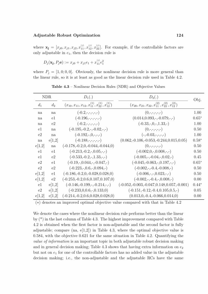
Adjustable Robust Optimization 124
where xj = [xj0, xj1, xj2, x(j)11 , x
(j)12 , x
(j)22 ]. For example, if the controllable factors are
only adjustable in e1, then the decision rule is
Dj(xj, Pje) := xj0 + xj1e1 + x(j)
11 e21
where Pj = [1, 0; 0, 0]. Obviously, the nonlinear decision rule is more general thanthe linear rule, so it is at least as good as the linear decision rule used in Table 4.2.
Table 4.3 – Nonlinear Decision Rules (NDR) and Objective Values
NDR D1(.) D2(.) Obj.d1 d2 (x10, x11, x12, x
(1)11 , x
(1)22 , x
(1)12 ) (x20, x21, x22, x
(2)11 , x
(2)22 , x
(2)12 )
na na (-0.2,-,-,-,-,-) (0,-,-,-,-,-) 1.00na e1 (-0.196,-,-,-,-,-) (0.014,0.093,-,-0.079,-,-) 0.65∗na e2 (-0.2,-,-,-,-,-) (-0.33,-,0,-,1.33,-) 1.00e1 na (-0.195,-0.2,-,-0.02,-,-) (0,-,-,-,-,-) 0.50e2 na (-0.192,-,0,-,-,-) (-,-0.03,-,-,-,-) 1.00na e[1,2] (-0.188,-,-,-,-,-) (0.062,-0.106,-0.053,-0.244,0.015,0.05) 0.58∗
e[1,2] na (-0.178,-0.2,0,-0.044,-0.044,0) (0,-,-,-,-,-) 0.50e1 e1 (-0.213,-0.2,-,0.05,-,-) (-0.002,0,-,0.008,-,-) 0.50e1 e2 (-0.533,-0.2,-,1.33,-,-) (-0.005,-,-0.04,-,0.02,-) 0.45e2 e1 (-0.19,-,0.044,-,-0.047,-) (-0.045,-0.063,-,0.197,-,-) 0.65∗e2 e2 (-0.223,-,0.6,-,0.094,-) (-0.002,-,-0.4,-0.008,-) 0.50
e[1,2] e1 (-0.186,-0.2,0,-0.028,0.028,0) (-0.006,-,-,0.023,-,-) 0.50e[1,2] e2 (-0.253,-0.2,0.6,0.107,0.107,0) (-0.002,-,-0.4,-,0.008,-) 0.00
e1 e[1,2] (-0.146,-0.199,-,-0.214,-,-) (-0.052,-0.003,-0.047,0.148,0.057,-0.001) 0.44∗e2 e[1,2] (-0.233,0,0.6,-,0.133,0) (-0.151,-0.12,-0.4,0.105,0.5,-) 0.05
e[1,2] e[1,2] (-0.214,-0.2,0.6,0.028,0.028,0) (0.013,0,-0.4,-0.066,0.014,0) 0.00(∗) denotes an improved optimal objective value compared with that in Table 4.2
We denote the cases where the nonlinear decision rule performs better than the linearby (*) in the last column of Table 4.3. The highest improvement compared with Table4.2 is obtained when the first factor is non-adjustable and the second factor is fullyadjustable; compare (na, e[1,2]) in Table 4.3, where the optimal objective value is0.584, with the objective 0.621 for the same situation in Table 4.2. Quantifying thevalue of information is an important topic in both adjustable robust decision makingand in general decision making; Table 4.3 shows that having extra information on e2
but not on e1 for one of the controllable factors has no added value in the adjustabledecision making; i.e., the non-adjustable and the adjustable RCs have the same

Adjustable Robust Optimization 125
optimal objective at (na, e2) and (e2, na). On the other hand, having information one1 for one of the controllable factors yields improvement in the objective; see (na, e1)and (e1, na) in Table 4.3. Moreover, if d1 responds to both environmental factors, andd2 uses information on e2 only, then we obtain the lowest possible optimal objectivevalue (namely, zero); see (e[1,2], e2) in Table 4.3.
Cell-Based Decision Rule
Now we propose a new type of decision rule that we call the cell-based decision rule:
Dj(xj, e) := xji if e ∈ cell(i), i ∈ Vj, (4.33)
where xj is the decision vector for the jth adjustable variable (xji being the decisionfor the ith cell), cell(i) is the region determined by the ith cell, and Vj is the set ofcell indices for the associated information-base.
Remark 11 Cells used in the decision rule are non-intersecting squares in two di-mensions, cubes in three dimensions, and hypercubes in higher dimensional uncer-tainty spaces. For the sake of simplicity, we assume that all cells have the samevolume (unless some cells are not merged to include enough data points).
If in the illustrative example (4.29), d1 is fully adjustable and the uncertainty set isdivided into four cells, then the decision rule is
D1(x1, e) :=
x11, e ∈ cell(1)x12, e ∈ cell(2)x13, e ∈ cell(3)x14, e ∈ cell(4)
(4.34)
where cell(i) := (e1, e2) ∈ R2 : `1i ≤ e1 ≤ u1i, `2i ≤ e2 ≤ u2i (i ∈ 1, 2, 3, 4),`1 = [0,−1,−1, 0], u1 = [1, 0, 0, 1], `2 = [0, 0,−1,−1], u2 = [1, 1, 0, 0], and V1 =1, 2, 3, 4; cells are represented by their center points in (4.30). To show the differ-ence between full and partial information, we assume that d1 is adjustable on e1 butnot on e2. The associated decision then becomes
D1(x1, e1) :=x11, e1 ∈ cell(1)x12, e1 ∈ cell(2) (4.35)
where cell(1) := e1 ∈ R : 0 ≤ e1 ≤ 1 and cell(2) := e1 ∈ R : −1 ≤ e1 ≤ 0, andV1 = 1, 2). It is easy to see that (4.35) implies that when e2 is extracted from theinformation-base, the new cells are projections from the cells in the two-dimensionalspace in (4.34) onto the one-dimensional space on e1 in (4.35). The disadvantage ofthe cell-based decision rule is that this rule often has more variables compared with

Adjustable Robust Optimization 126
the linear and nonlinear decision rules, especially when the number of cells is high.Nevertheless the numerical results for the example show that the new decision ruleis better than the linear, and is ‘almost’ as good as the nonlinear decision rule—evenwhen the total number of cells is only four; see Table 4.4.
Table 4.4 – Cell-Based Decision Rules (CDR) and Objective Values
CDR D1(.) D2(.) Obj.d1 d2 (x11, x12, x13, x14) (x21, x22, x23, x24)
na na (-0.2,−,−,−) (0,−,−,−) 1.00na e1 (-0.19,−,−,−) (-0.06,0.04,−,−) 0.66na e2 (-0.2,−,−,−) (0,0,−,−) 1.00e1 na (-0.3,-0.1,−,−) (0,−,−,−) 0.50e2 na (-0.2,-0.2,−,−) (0,−,−,−) 1.00na e[1,2] (-0.19,−,−,−) (-0.09,0.03,0.07,-0.05) 0.62
e[1,2] na (-0.3,-0.1,-0.1,-0.3) (0,−,−,−) 0.50e1 e1 (-0.3,-0.1,−,−) (0,0,−,−) 0.50e1 e2 (-0.3,-0.1,−,−) (-0.02,0.02,−,−) 0.45e2 e1 (-0.18,-0.2,−,−) (-0.06,0.04,−,−) 0.65e2 e2 (0.1,-0.5,−,−) (-0.2,0.2,−,−) 0.50
e[1,2] e1 (-0.3,-0.1,-0.1,-0.3) (0,0,−,−) 0.50e[1,2] e2 (0,0.2,-0.4,-0.6) (-0.2,0.2,−,−) 0.00
e1 e[1,2] (-0.3,-0.1,−,−) (-0.02,-0.02,0.02,0.02) 0.45e2 e[1,2] (0.1,-0.5,−,−) (-0.26,-0.14,0.26,0.14) 0.05
e[1,2] e[1,2] (0,0.2,-0.4,-0.6) (-0.2,-0.2,0.2,0.2) 0.00
To the best of our knowledge, parametric decision rules in the RO literature cannothandle adjustable integer variables, since the adjustable decision is a function of theuncertain parameter e, and the function does not necessarily take integer values forall e; see (4.31) and (4.32). However, the cell-based decision rule can handle suchvariables. As we can see from (4.33), the adjustable decision xji can take integervalues since the cell-based decision rule relates e and xij through an ‘if’ statement.Therefore, if we make xij an integer variable, then the cell-based decision rule givesinteger decisions. Note that similar decision rules have also been proposed by Bert-simas and Caramanis (2010); Hadjiyiannis et al. (2011); Vayanos et al. (2011).
Now using the illustrative example, we show the validity of our approach for ad-justable integer variables. We modify the old example in the following way: we

Realistic Examples 127
assume d1 and d2 are adjustable, and they take values that are multiples of 1/4.
Table 4.5 – Integer Cell-Based Decision Rules and Objective Values
CDR D1(.) D2(.) Obj.d1 d2 (x11, x12, x13, x14) (x21, x22, x23, x24)
na na (-0.25,−,−,−) (0,−,−,−) 1.41na e1 (-0.25,−,−,−) (0,0,−,−) 1.41na e2 (-0.25,−,−,−) (0,0,−,−) 1.41e1 na (-0.25,0,−,−) (0,−,−,−) 0.92e2 na (-0.25,-0.25,−,−) (0,−,−,−) 1.41na e[1,2] (-0.25,−,−,−) (0,0,0,0) 1.41
e[1,2] na (-0.25,0,0,-0.25) (0,−,−,−) 0.92e1 e1 (-0.25,0,−,−) (0,0,−,−) 0.92e1 e2 (-0.25,0,−,−) (0,0,−,−) 0.92e2 e1 (-0.25,-0.25,−,−) (0,0,−,−) 1.41e2 e2 (0.25,-0.5,−,−) (-0.25,0.25,−,−) 1.29
e[1,2] e1 (-0.25,0,0,-0.25) (0,0,−,−) 0.92e[1,2] e2 (0,0.25,-0.50,-0.75) (-0.25,0.25,−,−) 0.26
e1 e[1,2] (-0.25,0,−,−) (0,0,0,0) 0.92e2 e[1,2] (0,-0.50,−,−) (-0.25,0,0.25,0.25) 0.99
e[1,2] e[1,2] (0,0.25,-0.50,-0.75) (-0.25,-0.25,0.25,0.25) 0.26
Table 4.4 presents optimal decision rules and resulting objective values for all possiblecombinations of adjustability. These numerical results show that we obtain importantimprovements for the non-adjustable (na, na) optimal objective value by using thecell-based decision rule. As may be anticipated, the integer formulation yields higher(worse) optimal objective values. For example, we can no longer get a zero objectivein Table 4.5. Moreover, in contrast to the continuous case, we can no longer improvethe optimal objective of the non-adjustable RC at decision rule combinations: (na,e1), (na, e[1,2]), and (e2, e1); see the corresponding rows of Tables 4.4 and 4.5.
4.5 Realistic ExamplesIn this section, we present realistic examples to demonstrate the effectiveness of ourmethods. We use a 64-bit Windows PC with a 2.2 GHz Intel Core i7 processor, and8 GB of RAM. To solve the mathematical optimization problems, we use KNITRO8.0 embedded in MATLAB (2012a) and AIMMS 3.12.
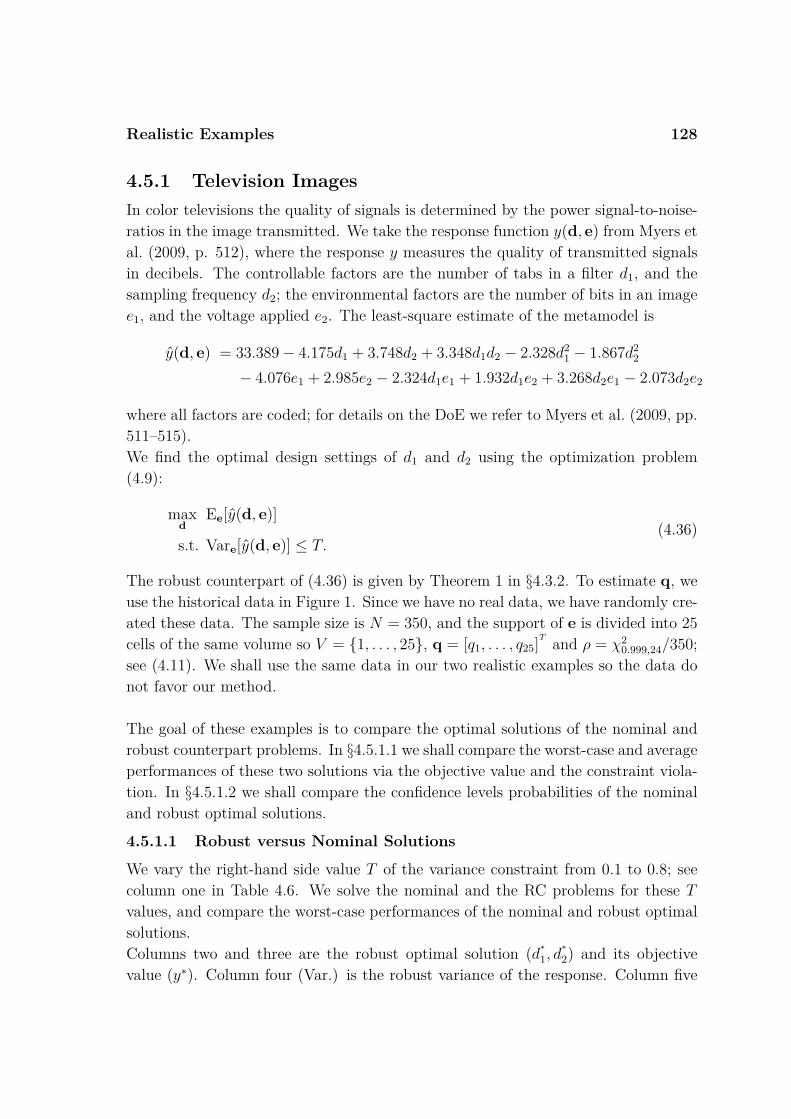
Realistic Examples 128
4.5.1 Television ImagesIn color televisions the quality of signals is determined by the power signal-to-noise-ratios in the image transmitted. We take the response function y(d, e) from Myers etal. (2009, p. 512), where the response y measures the quality of transmitted signalsin decibels. The controllable factors are the number of tabs in a filter d1, and thesampling frequency d2; the environmental factors are the number of bits in an imagee1, and the voltage applied e2. The least-square estimate of the metamodel is
y(d, e) = 33.389− 4.175d1 + 3.748d2 + 3.348d1d2 − 2.328d21 − 1.867d2
2
− 4.076e1 + 2.985e2 − 2.324d1e1 + 1.932d1e2 + 3.268d2e1 − 2.073d2e2
where all factors are coded; for details on the DoE we refer to Myers et al. (2009, pp.511–515).We find the optimal design settings of d1 and d2 using the optimization problem(4.9):
maxd
Ee[y(d, e)]
s.t. Vare[y(d, e)] ≤ T.(4.36)
The robust counterpart of (4.36) is given by Theorem 1 in §4.3.2. To estimate q, weuse the historical data in Figure 1. Since we have no real data, we have randomly cre-ated these data. The sample size is N = 350, and the support of e is divided into 25cells of the same volume so V = 1, . . . , 25, q = [q1, . . . , q25]T and ρ = χ2
0.999,24/350;see (4.11). We shall use the same data in our two realistic examples so the data donot favor our method.
The goal of these examples is to compare the optimal solutions of the nominal androbust counterpart problems. In §4.5.1.1 we shall compare the worst-case and averageperformances of these two solutions via the objective value and the constraint viola-tion. In §4.5.1.2 we shall compare the confidence levels probabilities of the nominaland robust optimal solutions.
4.5.1.1 Robust versus Nominal Solutions
We vary the right-hand side value T of the variance constraint from 0.1 to 0.8; seecolumn one in Table 4.6. We solve the nominal and the RC problems for these Tvalues, and compare the worst-case performances of the nominal and robust optimalsolutions.Columns two and three are the robust optimal solution (d∗1, d
∗2) and its objective
value (y∗). Column four (Var.) is the robust variance of the response. Column five

Realistic Examples 129
−1 −0.8 −0.6 −0.4 −0.2 0 0.2 0.4 0.6 0.8 1−1
−0.8
−0.6
−0.4
−0.2
0
0.2
0.4
0.6
0.8
1
e1
e 2
Figure 4.1 – Historical Data on e
Table 4.6 – Worst-Case Analysis for TV Image Example
TRobust Nominal
(d∗1, d∗2) y∗ Var.(%) (d∗1, d
∗2) W-C(E) W-C(Var)(%)
0.1 (-0.43,0.83) 35.27 0.10(0%) (-0.4472,0.7755) 35.27 0.19(88%)0.2 (-0.44,0.79) 35.28 0.15(-25%) (-0.4625,0.6853) 35.26 0.37(87%)0.3 (-0.44,0.79) 35.28 0.15(-50%) (-0.4763,0.6152) 35.23 0.56(86%)0.4 (-0.44,0.79) 35.28 0.15(-62%) (-0.4867,0.5648) 35.20 0.71(79%)0.5 (-0.44,0.79) 35.28 0.15(-70%) (-0.4867,0.5648) 35.20 0.71(43%)0.6 (-0.44,0.79) 35.28 0.15(-75%) (-0.4867,0.5648) 35.20 0.71(19%)0.7 (-0.44,0.79) 35.28 0.15(-78%) (-0.4867,0.5648) 35.20 0.71( 2%)0.8 (-0.44,0.79) 35.28 0.15(-81%) (-0.4867,0.5648) 35.20 0.71(-11%)
is the nominal optimum solution. Column six presents the mean (Ee[y(e,d)]) whenthe decision factors are fixed to the nominal optimum solution d∗ and the worst-caseprobability vector p∗ that minimizes the expectation is realized. Column seven (W.-C.(Var)) gives the worst-case value of the variance for the nominal solution; now weconsider the probability vector p∗ that maximizes the variance, as the worst-case.Notice that we also report the percentages of the worst-case constraint violations forthe nominal and robust optimal solutions; these values are shown within brackets(%) in the columns four and seven. We use the formula [(W.-C.(Var)-T ) × 100/T ]to calculate the constraint violation percentage of the nominal solution when theworst-case uncertain parameters are realized. If the violation percentage is negative,then the constraint is satisfied; 0% means the constraint is binding (see column four,

Realistic Examples 130
row T=0.1); a positive percentage means constraint violation at column seven.
Table 4.6 reveals that the robust reformulation of the variance constraint becomesredundant when T ≥ 0.2; e.g., the left-hand side value of the constraint for the ro-bust optimal solution (-0.4439,0.7988) when T = 0.2 is 0.149. Therefore we havethe same robust optimal solution for T ≥ 0.2. The nominal variance constraint (notthe worst-case) also becomes redundant when T ≥ 0.389, and therefore we have thesame nominal optimum solution when T ≥ 0.4. Notice that the robust optimal ob-jective values and the worst-case objective values of the nominal optimum solutionsare within 1% of each other. However, the constraint violation percentages favor ourrobust approach; e.g., the percentages in column seven show that when T ≤ 0.4, thenominal optimal solution violates the constraint on average 85% in the worst-case.When T ≥ 0.715 the nominal optimum solution no longer violates the constraint inthe worst-case, but it is closer to be binding than the robust solution. All together,using our robust optimization method for this example, we gain immunity to theworst-case uncertainty without being penalized by the objective.
Now we analyze the average mean and variance of the response for the nominal androbust optimal solutions, by randomly sampling 1,000 probability vectors p fromthe uncertainty set that is used in the RC; see (4.12). We sample as follows: Firstwe uniformly sample 25 individual probabilities (pi). Then to guarantee that theprobabilities sum up to one, we use the adjustment: pi = pi/
∑25j=1 pj. Finally, if the
probability vector p is within the uncertainty set, we keep p in the sample; else wediscard p and sample again. We repeat this procedure until we have 1,000 acceptedvectors that are within the set. The confidence level of the uncertainty set (4.12) is99.9%. From the p in the sample we estimate the mean in (4.14) and the variancein (4.16) for a given solution, and then take the averages; see Table 4.7.
Table 4.7 – Average (Avg) Mean (E) and Variance (Var)
TRobust Nominal
Avg(E) Avg(Var) Avg(E) Avg(Var)
0.1 35.37 0.064 35.41 0.120.2 35.40 0.095 35.45 0.240.3 35.40 0.095 35.46 0.350.4 35.40 0.095 35.47 0.46
Table 4.7 shows that the average expected response for the nominal solutions are

Realistic Examples 131
less than 1% better than that of the robust solutions (we maximize E(y); see (4.29)).Nevertheless, the average response variances of the robust optimal solutions are morethan 100% better (smaller) than that of the nominal solutions when T ≤ 0.2, andthe improvement becomes more than 350% when T ≥ 0.3. Moreover, we found thaton average the nominal solutions violate 5% of the variance constraint, whereas therobust solutions are not at all binding. The effectiveness of our approach is furtheranalyzed in the following subsection.
4.5.1.2 Confidence Level
The uncertainty set (4.12) coincides with the (1−α)-confidence set for the unknownprobability vector p centered at the empirical estimate q. In the numerical exampleswe use α = 0.001, which means that the robust optimal solution is immune touncertainty with at least 99.9% probability. These uncertainties are ignored in thenominal problem; nevertheless, the nominal solution may be robust for some part ofthe uncertainty set. To find the confidence level of a nominal solution, we calculatethe tightest uncertainty set for which the nominal solution at hand is robust; i.e., weadjust the ρ value in (4.12); see Table 4.8.
Table 4.8 – Confidence Levels (1-α) of Nominal Solutions
T ≤ 0.4 0.5 0.6 0.7 ≥ 0.8
(1− α) 0% 2% 70% 98% 99.9%
Table 4.8 shows that when T ≤ 0.4 the nominal solutions have no immunity to un-certainty at all; i.e., a ‘small’ change in the given empirical estimate q results ininfeasibility in the nominal variance constraint. We may anticipate this result, sincethe nominal solutions are binding for the associated cases. On the other hand, forT = 0.5 to T = 0.7 we see important improvement in the immunity to uncertainty forthe nominal solution. In addition, when T ≥ 0.8, the immunity of the nominal opti-mum solution is as good as the robust optimum solution—even though the nominaloptimum solution is closer to be binding in the constraint than the robust solution.Concerning the objective, we have already shown in the last row of Table 4.6 thatthe robust and the ‘worst-case’ nominal optimum objective values are almost thesame; i.e., the robust solutions are less than 1% better than the nominal solutions.In conclusion, the robust reformulation improves the immunity to uncertainty whenT ≤ 0.8 and the improvement is even better when T ≤ 0.4. Additionally, we preferthe robust solution when T ≥ 0.8, since it performs better in the worst-case.
Realistic Examples 132
4.5.2 Distribution CenterIn this example we focus on the simulation of a cross-docking distribution center(CDDC) developed by Shi (2011). The CDDC is used by a Chinese automobile man-ufacturer that needs to improve the physical flow in its supply chain. The objectiveof the company is steady production. The challenge in such production is the supplyuncertainty due to environmental factors, mentioned below. To model the associatedsupply chain system, Shi proposes a hybrid approach that combines discrete-eventsimulation, RSM, and Taguchi’s world view. We focus on Shi’s linear regressionmetamodel for the total throughput with five controllable factors; namely, the num-ber of receiving doors d1, the number of shipping doors d2, the number of forkliftsd3, the number of conveyors d4, and the supply chain threshold in storage d5. Themodel has two environmental factors; namely, the variability in less-than-truckloadsupply shipments e1, and the production interruption or delay probabilities of thesuppliers e2. Using the simulation’s I/O data, Shi approximates the unknown I/Ofunction of the total throughput by the following least-squares estimate y:
yTT(e,d) =104 ×[47.97 + 3.982d1 + 2.025d2 − 0.031d3 + 0.734d4 + 0.034d5
+ 0.789d1d2 + 0.012d1d3 + 0.003d1d4 − 0.002d1d5 + 0.0007d2d3
− 0.065d2d4 − 0.1131d2d5 − 0.078d3d4 − 0.041d3d5 + 0.11d4d5
− 3.406d2
1 − 1.781d2
2 + 0.011d2
3 − 1.033d2
4 + 0.111d2
5
+ (16.66 + 1.511d1 + 2.374d2 − 0.059d3 + 0.824d4 − 0.093d5)e1
− (0.005 + 0.27d1 + 0.661d2 − 0.086d3 + 0.335d4 − 0.005d5)e2
],
where all factors are coded such that −1 ≤ d ≤ 1, and −1 ≤ e ≤ 1. More precisely,the coded controllable factors are between -1 and 1 because of the physical restric-tions of the production facility. Shi’s ANOVA shows that the metamodel yTT havenon-significant lack-of-fit; and for the estimated parameters the level-of-significanceis 0.05. Using Shi’s response model, we focus on the robust reformulation of thefollowing optimization problem:
min1≤d≤1
Vare[y(d, e)]
s.t. Ee[y[d, e)] ≥ T.(4.37)
To estimate the frequencies q used by the nominal and RC problems, we use thesame historical data as in Figure 4.1.
Table 4.9 compares the worst-case performances of the nominal and robust optimalsolutions. Besides the worst-case mean and standard deviation, we construct the

Realistic Examples 133
Table 4.9 – Worst-Case Comparison for CDDC Example
TRobust Nominal (Worst-Case)
σe(y) Ee[y] Ee[y]± 3σe σe(y) Ee[y] Ee[y]± 3σe
≤339 67 339 (136, 541) 67 339 (136, 541)340 67 340 (137, 542) 67 339 (136, 541)370 70 370 (158, 581) 68 348 (143, 552)400 74 400 (176, 623) 71 377 (163, 590)420 79 420 (182, 657) 73 396 (174, 617)430 81 430 (184, 675) 75 405 (178, 632)440 85 440 (184, 695) 77 414 (181, 648)450 88 450 (183, 716) 80 424 (183, 664)∗ ∗ ∗ all entries should be multiplied by 1,000
worst-case confidence interval for y; namely, Ee[y] ± 3σe. Because the probabilitydistribution of the environmental factors is unknown, we cannot say much about theconfidence level of this interval. The numerical results show that in the worst-casethe nominal solutions are on average 6% lower than the target T for the expectedtotal throughput; i.e., the average violation of the constraint is 6%. The worst-casestandard deviations of the total throughput for the nominal solutions are on average8% lower than that of the robust ones. Nevertheless the confidence intervals for therobust optimal solutions are always shifted to the right compared with the nominalsolutions, which is in favor of the robust approach since a higher total throughput isbetter. Altogether the numerical results favor the robust approach when T >339000;when T ≤ 339000 both methods yield the same outcome.
In Table 4.10 we compare the average performance of robust and nominal solutionsvia Monte Carlo simulation. First, using the given historical data in Figure 4.1 asthe nominal value (q) of the uncertainty set, we generate 1,000 probability vectors,like we did for the TV images example. Then we calculate the expected responseand variance for the nominal and robust solutions at each probability vector, andtake the averages. Table 4.10 shows higher means and lower variances than Table4.9 in the worst-case. Table 4.9 is based on the worst-case scenario; i.e., we maxi-mize the variance and minimize the expectation; Table 4.10 is based on the averageperformance. Table 4.10 shows that the confidence intervals for the robust solutionsare always shifted to the right compared with the nominal solutions, so we prefer therobust approach, however, the robust solutions have slightly higher variations (from

Realistic Examples 134
Table 4.10 – Average Comparison for CDDC Example (Simulation Results)
TRobust Nominal
σe(y) Ee[y] Ee[y]± 3σe σe(y) Ee[y] Ee[y]± 3σe
≤339 58 361 (186, 536) 58 360 (185, 535)340 58 361 (186, 536) 58 360 (185, 535)370 61 392 (209, 575) 59 369 (192, 547)400 64 423 (229, 618) 61 399 (214, 585)420 68 445 (238, 652) 64 419 (227, 612)430 71 456 (241, 670) 65 429 (232, 627)440 74 467 (244, 690) 67 439 (236, 643)450 77 478 (245, 711) 69 449 (239, 659)∗ ∗ ∗ all entries should be multiplied by 1,000
0% to 10%) than the nominal solutions.
Adjustable Robust Optimization
One of the most important decision factors in the CDDC is the number of shippingdoors d2. A moderate number of shipping doors may increase the inventory in thetemporary storage area, whereas an excessive number causes a low utilization ofdoors. We now assume that d2 is adjustable according to the uncertain parametere1—namely, the variability in less-than-truckload supply shipments. More precisely,we assume that the number of shipping doors can be adjusted after the variability insupply shipments has been observed. We use the cell-based decision rule introducedin §4.4; the data and the 25 cells are presented in Figure 4.1. Notice that the domainof e1 is divided into five equal intervals; for each interval we have a different decision.In Table 4.11, columns two through four present the actual ‘worst-case’ performanceof the ARC, and columns five through eight present the average performance of ad-justable robust solutions via Monte Carlo simulation as in Table 4.10. We use thesame probability vector sample as in the television images example. These numericalresults show that the worst-case confidence intervals of the ARC are tighter thanthose of the general RC in Table 4.9. This is because of the improved responsevariances of the adjustable robust solutions, the improvement percentages (%) arereported in column two within brackets; e.g., it is as high as 10% when T =450000.As we anticipated, the simulation results show that the average performance of theadjustable robust solutions is better than the worst-case; i.e., the average of the re-sponse mean Ee[y] is higher than the worst-case mean Ee[y], and the average varianceσe(y)2 is lower than the worst-case variance σe(y)2. Comparing the average perfor-

Conclusions and Future Research 135
Table 4.11 – ARO Results for CDDC Example
Worst-Case Average
T σe(y) Ee[y] Ee[y]± 3σe σe(y) Ee[y] Ee[y]± 3σe
≤339 67 (0%) 339 (136, 541) 58 367 (192, 541)340 67 (0%) 340 (137, 542) 58 367 (193, 542)370 68 (2%) 370 (167, 572) 59 389 (194, 543)400 71 (3%) 400 (188, 611) 61 418 (212, 566)420 73 (6%) 420 (201, 639) 63 425 (235, 615)430 74 (7%) 430 (209, 650) 64 448 (246, 630)440 75 (10%) 440 (215, 665) 65 449 (254, 644)450 78 (10%) 450 (216, 684) 69 456 (249, 661)∗ ∗ ∗ all entries should be multiplied by 1,000
mances of the non-adjustable and adjustable robust solutions in Tables 4.10 and 4.11shows that the ARC yields tighter confidence intervals that are subintervals of theconfidence intervals in the general RC. Therefore, the ARC reduces the response un-certainty compared with the general RC. Finally, additional experimentation showedthat making ‘only’ d3, d4 or d5 adjustable on e1 has an improvement less than 1%in the objective; i.e., in those cases the non-adjustable solutions are as good as theadjustable solutions. This shows that the quantitative value of information maysignificantly change for different parameters in ARO.
4.6 Conclusions and Future ResearchIn this chapter, we proposed a RO methodology for RPD, this methodology uses anuncertainty set based on historical data on the environmental variables; data may becollected from either real or simulated systems. Adding RO to RPD has the followingadvantages: (i) Unlike the classical RPD, we do not make any distributional assump-tions on the uncertain parameters. (ii) We do account for the ambiguity caused by thelack of knowledge about distributions by using the so-called φ-divergence uncertaintysets based on historical data. (iii) Both RO and ARO methods are computationallytractable; ARO is tractable even for nonlinear decision rules. (iv) Our ARO approachcan be used for modeling adjustable integer decision variables. In future research, weshall apply the cell-based decision rules to general classes of optimization problemswith moderate numbers of ‘integer’ variables.

Bibliography
Al-Aomar, R. 2006. Incorporating robustness into genetic algorithm search of stochas-tic simulation outputs. Simulation Modelling Practice and Theory 14(3) 201–223.
Angun, E. 2011. A risk-averse approach to simulation optimization with multipleresponses. Simulation Model. Practices and Theory 19(3) 911–923.
Ben-Tal, A., A. Nemirovski. 1998. Robust convex optimization. Math. Oper. Res.23(4) 769–805.
Ben-Tal, A., A. Nemirovski. 1999. Robust solutions of uncertain linear programs.Oper. Res. Lett. 25(1) 1–13.
Ben-Tal, A., D. den Hertog, J.-P. Vial. 2014. Deriving robust counterparts of non-linear uncertain inequalities. Math. Prog. forthcoming.
Ben-Tal, A., L. El Ghaoui, A. Nemirovski. 2009. Robust Optimization. PrincetonPress, Princeton, NJ.
Ben-Tal, A., D. den Hertog, A. De Waegenaere, B. Melenberg, G. Rennen. 2013. Ro-bust solutions of optimization problems affected by uncertain probabilities. Man-agement Sci. 59(2) 341–357.
Bertsimas, D., C. Caramanis. 2010. Finite Adaptability in Multistage Linear Opti-mization. IEEE Transactions on Automatic Control 55(12) 2751–2766.
Bertsimas, D., O. Nohadani, K. M. Theo. 2010. Robust optimization for uncon-strained simulation-based problems. Oper. Res. 58(1) 161–178.
Bingham, D., V. N. Nair. 2012. Noise variable settings in robust design experiments.Technometrics 54(4) 388–397.
Chan, Y.-J., D. J. Ewins. 2010. Management of the variability of vibration responselevels in mistuned bladed discs using robust design concepts. Mech. Systems andSignal Processing Part 1: Parameter Design 24(8) 2777–2791.
Dasgupta, T., C. F. J. Wu. 2006. Robust Parameter design with feed-back control.Technometrics 48(3) 349–359.
Dellino, G., J. P. C. Kleijnen, C. Meloni. 2012. Robust optimization in simulation:Taguchi and Krige combined INFORMS J. Comput. 24(3) 471–484.
Delpiano, J., M. Sepulveda. 2006. Combining iterative heuristic optimization and

BIBLIOGRAPHY 137
uncertainty analysis methods for robust parameter design. Engineering Optim.38(7) 821–831.
El-Ghaoui, L., H. Lebret. 1997. Robust solutions to least-squares problems withuncertain data. SIAM. J. Matrix Anal. & Appl. 18(4) 1035–1064.
Fu, M. C. 2007. Are we there yet? The marriage between simulation & optimization.OR/MS Today 34(3) 16–17.
Fu, M., B. Nelson. 2003. Simulation optimization. ACM Trans. Model. and Simula-tion 13(2) 105–107.
Hadjiyiannis, M. J., P. Goulart, D. Kuhn. 2011. A scenario approach for estimatingthe suboptimality of linear decision rules in two-stage robust optimization Pro-ceedings of the Decision and Control and European Control, 50th IEEE Conference7386–7391.
Hu, Zhaolin, J. Cao, L. J. Hong. 2012. Robust simulation of global warming policiesusing the DICE model. Management Sci. 58(13) 2190–2206.
Iman, R. L., J. C. Helton. 2006. An investigation of uncertainty and sensitivityanalysis techniques for computer models. Risk Anal. 8(1) 71–90.
Joseph, V. R. 2003. Robust parameter design with feed-forward control. Technomet-rics 45(4) 284–292.
Kleijnen, J. P. C. 2008. Design and Analysis of Simulation Experiments. Springer-Verlag, Heidelberg, Germany.
Miranda, A. K., E. Del Castillo. 2011. Robust parameter design optimization ofsimulation experiments using stochastic perturbation methods. J. Oper. Res. Soc.62(1) 198–205.
Myers, R. H., D. C. Montgomery, C. M. Anderson-Cook. 2009. Response SurfaceMethodology: Process and Product Optimization Using Designed Experiments, 3rded. John Wiley & Sons, Hoboken, NJ.
Nair, V. N., B. Abraham, J. MacKay, G. Box, R. N. Kacker, T. J. Lorenzen, J. M.Lucas. 1992. Taguchi’s parameter design: a panel discussion. Technometrics 34(2)127–161.
Pardo, L. 2006. Statistical Inference Based on Divergence Measures. Chapman &Hall/CRC, Boca Raton, FL.
Rockafellar, R. T. 1970. Convex Analysis. Princeton University Press, Princeton, NJ.Sanchez, S. M. 2000. Robust design: seeking the best of all possible worlds. Pro-
ceedings of the 2000 Winter Simulation Conference (edited by J.A. Joines, R.R.Barton, K Kang, and P.A. Fishwick) 1 69–76.
Shi, W. 2011. Design of pre-enhanced cross-docking distribution center under sup-ply uncertainty: RSM robust optimization method. Working Paper, Huazhong

BIBLIOGRAPHY 138
University of Science & Technology, China.Spall, J. 2003. Introduction to Stochastic Search and Optimization. Wiley-
Interscience, New York, NY.Stinstra, E., D. den Hertog. 2008. Robust optimization using computer experiments.
EJOR 191(3) 816–837.Taguchi, G. 1986. Introduction to Quality Engineering. Asian Productivity Organi-
zation, UNIPUB, White Plains, NY.Taguchi, G. 1987. System of Experimental Design: Engineering Methods to Optimize
Quality and Minimize Cost. UNIPUB/Kraus International, White Plains, NY.Urval, R., S. Lee, S. V. Atre, S.-J. Park, R. M. German. 2010. Optimisation of process
conditions in powder injection moulding of microsystem components using robustdesign method. Powder Metallurgy Part 2: Secondary Design Parameters 53(1)71–81.
Vanlı, O. A., E. Del Castillo. 2009. Bayesian approaches for on-line robust parameterdesign. IIE Transactions 41(4) 359–371.
Vayanos, P., D. Kuhn, B. Rustem. 2011. Decision rules for information discoveryin mutli-stage stochastic programming. Proc. 50th IEEE Conf. on Decision andControl and European Control Conf. (CDC-ECC), Orlando, FL, 7368–7373.
Wiedemann, M. 2010. Robust Parameter Design for Agent-Based Simulation ModelsWith Application in a Cultural Geography Model. Master’s Thesis, Naval Post-graduate School, Monterey, CA.
Yanıkoglu, I., D. den Hertog. 2013. Safe approximations of ambiguous chance con-straints using historical data. INFORMS J. Comput. 25(4) 666–681.

CHAPTER 5
Robust Pessimistic Bilevel Optimization
5.1 Introduction
“Good optimization gives you the best choice based on the data. Greatoptimization is robust and resilient in the face of change and data errors.”Sashihara (2011)
Optimization problems often contain uncertain parameters because of measurement,estimation, and implementation errors. There are two novel optimization approachesfor handling such errors, namely, robust and stochastic optimization. To model un-certain parameters, robust optimization (RO) uses uncertainty sets; and stochasticoptimization (SO) uses probability distributions. Due to this basic difference, thetwo methods may significantly differentiate from each other. In this chapter we workon a class of uncertain optimization problems, where SO and RO coincide with eachother, i.e., the associated modelling issue is not important when certain assumptionson uncertainty hold. However, in the sequel of the chapter, we generally adopt theRO terminology, and we shall use some of the techniques that are mainly inventedin the realm of RO, and later extended to SO.
RO is a relatively young and active research field that is mainly developed in thecourse of the last 15 years. As it is explained above, the goal of RO is to find so-lutions that are robust with respect to the uncertainty of the problem parametersin a given mathematical optimization problem. It requires that the constraints of agiven problem should be satisfied for all realizations of the uncertain parameters in aso-called uncertainty set. The robust version of a mathematical optimization prob-lem is generally referred to as the robust counterpart (RC) problem. RO is popularbecause of the tractability of the RC for many classes of uncertainty sets, and itsapplicability in real life.

Introduction 140
Adjustable robust optimization (ARO) distinguishes between two types of decisionvariables, namely, “wait and see” or “here and now”. More precisely, decisions on“here and now” variables must be made before the uncertain parameters are realizedlike in classical RO; whereas decisions on “wait and see” variables are made aftersome or all of the uncertain parameters reveal themselves. ARO relates “wait andsee” variables to uncertain parameters using decision rule functions; for additionaldetails, we refer to (Ben-Tal et al., 2009, Chapter 14). In this chapter, we proposean ARO approach for a class of bilevel optimization problems. We assume that thefirst stage decisions are “here and now”, and the later stage decisions are “wait andsee”, i.e., they are adjustable according to a realized portion of the uncertain data.It is important to point out that bilevel optimization problems that we shall considerin this chapter are in general computationally intractable, but by using modern ROtechniques we provide practable approximations of the associated problems.
Bilevel optimization (BO) problems involve two nested traditional optimization prob-lems with conflicting objectives. These two optimization problems are often referredto as the upper-level and the lower-level problems. The standard formulation is asfollows
minx∈X , y∈Y (x)
f(x, y) where Y (x) = argminz∈Z(x) h(x, z), (5.1)
where x ∈ X ⊆ Rn is the upper-level decision, y ∈ Y (x) ⊆ Z(x) ⊆ Rm is the lower-level decision, X is the set of feasible solutions of the upper-level problem, Z(x) isthe set of feasible solutions of the lower-level problem that are dependent on theupper-level decision x, and f, h : X×Y → R. Using the optimal value reformulationDempe and Zemkoho (2013); Mitsos et al. (2008), (5.1) can be reformulated as thefollowing single-level problem:
minx∈X , y∈Z(x)
f(x, y) s.t. h(x, y) ≤ h∗(x), (5.2)
where h∗(x) = min h(x, y) : y ∈ Z(x). If the lower-level optimization problem isconvex, then the most common approach is to replace this problem with the associ-ated Karush-Kuhn-Tucker (KKT) conditions in order to obtain the explicit single-level reformulation. Nevertheless, the associated reformulation is often non-convexeven for the linear case of the bilevel problem. Therefore, to solve these complexproblems, global optimization algorithms are needed; for details of such algorithms,we refer to Faısca et al. (2007); Mitsos et al. (2008); Tsoukalas et al. (2009), and Tuyet al. (2007).

Introduction 141
Even though bilevel optimization problems are computationally complex, they havemany applications in real life. History of bilevel problems dates back to the 1930s,the seminal work of von Stackelberg proposes a bilevel problem to find the mar-ket equilibria in an economic model; see in Tirole and Fudenberg (1991). Fortyyears later, Bracken and McGill (1973) formalize bilevel problems as optimizationproblems. In the recent twenty years, such optimization problems have been ap-plied to various fields, e.g., revenue management (Cote et al., 2003), supply chainmanagement (Ryu et al., 2004), production planning (Iyer and Grossmann, 1998),transportation (Migdalas, 1995), security (Scaparra and Church, 2008), power mar-kets (Zhang et al., 2011); and this list can be easily extended.
The pessimistic bilevel optimization problem that slightly deviates from the standardformulation (5.1) is defined as
minx∈X
maxy∈Y (x)
f(x, y) where Y (x) = argminz∈Z(x) h(x, z), (5.3)
where the problem is called independent when Y (x) = Y (x′) for all x, x′ ∈ X ; anddependent when Y (x) 6= Y (x′) for some x, x′ ∈ X .
Note that the pessimistic problem (5.3) can be reformulated as
minx∈X ,τ
τ
s.t. τ ≥ f(x, y) ∀y ∈ Y (x) = argminz∈Z(x) h(x, z)(5.4)
using an epigraphic reformulation and “∀” that replaces the inner maximization.Wiesemann et al. (2013) propose convergent approximation techniques to solve in-dependent pessimistic optimization problems using semi-infinite programming undermild regularity assumptions.
It is important to point out that the pessimistic bilevel problem (5.3) is computation-ally more complex than the classical problem (5.1), and this is why most theoreticalcontributions to bilevel optimization are for the classical (optimistic) formulationthat replaces “∀” with “∃” in (5.4). Both pessimistic and optimistic formulationshave natural interpretations as non-cooperative games that are commonly referredto as the Stackelberg games between two players; for details again see Tirole andFudenberg (1991). A Stackelberg game is a sequential game, where the first player(the leader) chooses his decision x, and then the second player (the follower) observesx and reacts with a decision y. In the pessimistic formulation, the leader has limitedinformation about the optimal decision of the follower, and hence he wants to stay

Single-Level Reformulation 142
feasible for any rational decision of the follower. On the other hand, in the optimisticformulation, the leader may bias the decisions of the follower to some extent and thefollower altruistically favors the leader’s objective with her decisions. The optimalsolutions of the two formulations may significantly differ from each other.
In this chapter, we propose solution methods for a general pessimistic bilevel op-timization problem with uncertainty. This problem is computationally intractablebecause the follower problem may be nonconvex, and the problem contains uncer-tain parameters as well as dependent second stage decisions. To solve the associatedproblem, we propose conservative approximation methods that are based on primaland dual linear decision rules and some other RO techniques that shall be discussed inlater sections. The proposed technique simplifies the complex structure of the prob-lem and provides a more tractable reformulation that gives a conservative solution.To quantify the optimality performance of this solution, we also give an optimisticreformulation that yields an efficient lower bound for the original problem. As wellas being computationally less challenging, the associated reformulation method alsohas natural practical interpretations: first, the leader may have incomplete informa-tion about the follower decisions and this is why he may want to include some safetymargin with a conservative formulation. Second, the follower may be constrained bybounded rationality, i.e., she may not solve the lower-level problem to optimality. Inboth cases the leader may want to hedge against the worst-case decisions the followercan make by solving a conservative reformulation, and our solution method also fitsinto this practical perspective.
The remainder of the chapter is organized as follows. §2 presents single-level re-formulation methods for pessimistic bilevel optimization problems. §3 summarizesprimal and dual linear decision rules used in RO. §4 proposes an RO methodologyfor a class of pessimistic bilevel optimization problems. §5 presents a numericalexperiment. Finally, §6 summarizes our conclusions.
5.2 Single-Level ReformulationIn this section, we give a brief introduction on the reformulation techniques of pes-simistic bilevel optimization problems with certain data. For the sake of exposition,we adopt an implicit notation in this section. Later in §§3 and 4, we shall explicitlydwell in details of these reformulation techniques.
To begin with, using the optimal value reformulation, the pessimistic formulation

Primal and Dual Linear Decision Rules 143
(5.3) can be reformulated as
minx∈X
maxy∈Y (x)
f(x, y)
s.t. h(x, y) ≤ h∗(x),(5.5)
where h∗(x) = min h(x, y) : y ∈ Z(x) as in (5.2). Next, if the dual problem of theinner maximization problem in (5.5) satisfies the regularity conditions (in particular,it is a convex optimization problem), then it can be reformulated as
maxy∈Y (x)
f(x, y) s.t. h(x, y) ≤ h∗(x) = minλ
g(x, λ) s.t. λ ∈ Λ(x), (5.6)
where g(x, λ) denotes the dual objective value function, λ ∈ Λ(x) denotes the dualvariables, and Λ(x) is the set of dual feasible solutions for a given x ∈ X . Eventually,the pessimistic bilevel problem (5.3) can be reformulated as the single-level problem:
minλ, x∈X
g(x, λ) s.t. λ ∈ Λ(x). (5.7)
To point out, going from (5.3) to (5.5) is justified because the regularity condition isassumed to be satisfied for the lower-level problem, i.e., we can use the dual problemto explicitly formulate h∗(x). If the regularity condition is not met, then the lower-level problem can be replaced with KKT conditions but this yields a nonconvexand conservative reformulation of (5.3); see Mirrlees (1999). Similarly, going from(5.5) to (5.7) is justified only when the inner maximization problem (5.6) satisfiesthe constraint qualification, and it has a concave objective in y for any x ∈ X(e.g., when f(x, y) is additively separable in x and y). Eventually, we obtain thesingle level reformulation in (5.7), but it is important to point out that the resultingreformulation is often a nonconvex optimization problem unless there exists a specialconvexification technique like in §4.
5.3 Primal and Dual Linear Decision RulesIn this section, we give a brief overview of the primal and dual linear decision rulemethods used in stochastic and robust optimization. This chapter focuses on aspecific class of the uncertain optimization problems where a decision maker firstobserves a portion of the uncertain parameter ξ and then selects a decision y(ξ) ∈ Rn
that is subject to constraints Ay(ξ) ≤ b(ξ) with a cost c(ξ)>y(ξ). In SO, the goalis to find the optimal y(ξ) ∈ L2
k,n that minimizes the expected cost, where L2k,n is
the space of all Borel measurable, square-integrable functions from Rk to Rn. Such

Primal and Dual Linear Decision Rules 144
a decision y(ξ) is often referred to as “wait and see”; and the decision problem thatis mentioned above can be formulated as the following linear one-stage problem:
miny
Eξ[c(ξ)>y(ξ)]
s.t. Ay(ξ) ≤ b(ξ) Pξ-a.s.,(SP)
where the coefficients matrix A ∈ Rm×n is independent of ξ, i.e., the fixed recourse,and the constraints are satisfied almost surely with respect to Pξ, i.e., the underlyingprobability distribution of ξ. We assume that the objective function coefficients andthe right-hand side are linear in ξ, more precisely, c(ξ) = Cξ for some C ∈ Rn×k andb(ξ) = Bξ for some B ∈ Rm×k. In addition, we also assume that the support of theprobability distribution Pξ resides in a non-empty compact polyhedron:
Ξ =ξ ∈ Rk : Wξ ≥ h
(5.8)
for some matrix W ∈ Rl×k and a vector h ∈ Rl. Without loss of generality, weassume that ξ1 = 1 (∀ξ ∈ Ξ), i.e.,
W = (e1,−e1, W>)> and h = (1,−1, 0, . . . , 0)>,
where e1 denotes a basis vector in Rk. We use ξ1 = 1 to model the constant termsat affine functions.
It is known that optimizing SP is an NP-hard problem even when Pξ is a uniformdistribution on a unit cube; for details see Dyer and Stougie (2006, Theorem 3.2).Therefore, there is no polynomial time algorithm that solves this problem unless P= NP. Nevertheless Ben-Tal et al. (2004) propose a tractable approximation of SPby restricting the functional space of y(ξ) to linear decision rules. It is important topoint out that this complexity reduction method has been first proposed by Ben-Talet al. in the realm of RO. Later Chen et al. (2008) and Shapiro and Nemirovski(2005) extended the ideas of Ben-Tal et al. to SO.
5.3.1 Primal ApproximationAs it is mentioned above, a tractable approximation of SP is obtained by adoptinglinear decision rules, i.e., y(ξ) = Y ξ. The resulting problem contains a finite numberof decision variables and infinitely many constraints. Therefore, it is a semi-infiniteoptimization problem given as follows
minY ∈Rn×k
Tr(MC>Y )
s.t. AY ξ ≤ Bξ Pξ-a.s.,(5.9)

Primal and Dual Linear Decision Rules 145
where M := E[ξξ>] is the second-order moment matrix. Notice that (5.9) is an upperbound for SP since it restricts the feasible functional space of the decision rules.
Tractable reformulation of (5.9). If we assume that the support of the probabilitydistribution Pξ resides in the compact polyhedron Ξ given in (5.8), then (5.9) can beequivalently reformulated as
minY ∈Rn×k
Tr(MC>Y )
s.t. AY ξ ≤ Bξ ∀ξ ∈ Ξ(5.10)
Notice that (5.10) is also a semi-infinite optimization problem that seems to beintractable in its current form. However, it can be reformulated with a finite numberof constraints by using the RO paradigm; for details on deriving a tractable robustreformulation, i.e., the robust counterpart (RC) problem, we refer to Ben-Tal andNemirovski (1998), and Ben-Tal et al. (2009). Eventually (5.9) simplifies to thefollowing linear optimization problem (LP):
min Tr(MC>X)s.t. Y ∈ Rn×k,Λ ∈ Rm×l,Λ ≥ 0
AY + ΛW = B
Λh ≥ 0
(SPu)
where Λ is a matrix of auxiliary dual variables.
All in all, by adopting linear decision rules and using the RO paradigm, we obtain atractable reformulation SPu that constitutes an upper bound for SP .
5.3.2 Dual ApproximationThe dual problem of SP , provided in Wright (1994), is given as follows
infy,s≥0
supλ
Eξ[c(ξ)>y(ξ) + λ(ξ)>[Ay(ξ) + s(ξ)− b(ξ)]
](SPd)
where s(ξ) denotes the decision rules for the slack variables, infy,s≥0 denote the in-fimum over all y ∈ L2
k,n and over all s ∈ L2k,m that are almost surely nonnegative.
Similarly, supλ stands for the supremum over all y ∈ L2k,m. Notice that the feasible
functional spaces are kept general in SPd.
Similar to the complexity reduction techniques applied for the primal problem, Kuhnet al. (2011) propose adopting linear decision rules for the dual variables in SPd, more

Primal and Dual Linear Decision Rules 146
precisely, λ(ξ) = Λξ, that is given as follows
infy,s≥0
supΛ
Eξ[c(ξ)>y(ξ) + ξ>Λ>[Ay(ξ) + s(ξ)− b(ξ)]
]= inf
y,s≥0sup
ΛEξ[c(ξ)>y(ξ)
]+ Tr
(Λ>E
([Ay(ξ) + s(ξ)− b(ξ)]ξ>
)).
(5.11)
To point out, (5.11) constitutes a lower bound on the optimal objective value of SPsince it restricts the feasible functional space of the dual variables to a linear decisionrule in the dual problem. More precisely, the inner problem, i.e., the supremum,yields a lower optimal objective value (for a given y and s) compared to that inSPd since the dual decision rules are restricted to linear ones. Notice that, in order(5.11) to be well defined, E
([Ay(ξ) + s(ξ)− b(ξ)]ξ>
)= 0 must be satisfied, otherwise
we can select Λ in such a way that the supremum goes to infinity and the problembecomes infeasible. Therefore, we can reformulate (5.11) as the following semi-infiniteproblem:
miny,s
Eξ[c(ξ)>y(ξ)
]s.t.
Eξ[[Ay(ξ) + s(ξ)− b(ξ)]ξ>
]= 0
s(ξ) ≥ 0
Pξ-a.s. (or ∀ξ ∈ Ξ).(5.12)
Tractable reformulation of (5.12). Similar to the primal approximation, usingRO, Kuhn et al. (2011) propose an equivalent tractable reformulation of (5.12), whenthe support of Pξ is in a compact polyhedron (5.8). The tractable RC reformulationis given as follows
min Tr(MC>Y )s.t. Y ∈ Rn×k, S ∈ Rm×k
AY + S = B
(W − he>1 )MS> ≥ 0,
(SP l)
where M is the second-order moment matrix; for details on deriving SP l we refer toKuhn et al. (2011, §2.4).
Remark 12 Notice that we can quantify the loss of optimality incurred by usinglinear decision rules in SP by adopting linear decision rules to the dual problem. Inother words, SP l constitutes a lower bound on SPu, and the gap between val(SPu)and val(SP l) estimates the approximation error of adopting linear decision rules.

Robust Bilevel Optimization 147
5.4 Robust Bilevel OptimizationIn this section, we adopt primal and dual linear decision rules to approximate a classof bilevel optimization problems. The associated problem is a multi-stage uncertainoptimization problem with two decision makers, namely, the leader and the follower.The decision making process is sequential, in the first stage, the leader makes binary(0− 1) decisions x ∈ X ⊆ 0, 1g with a cost q>x before the uncertain data ξ ∈ Rk
reveals itself; at later stages, the follower observes an element ξ of the uncertaindata and makes a decision y′(ξ) ∈ L2
k,n with a cost c(ξ)>y′(ξ) and subject to theconstraints Ay′(ξ) ≤ b(x, ξ) that are dependent on the first stage decision x made bythe leader. The leader knows the possible decisions y(ξ) that the follower can select,and takes into account the worst-case cost v(ξ)>y(ξ) that may be imposed on himby the follower. The associated decision problem can be formulated as the followingbilevel optimization problem:
minx∈X
q>x+ maxy(.)
Exi[v(ξ)>y(ξ)]
s.t. y(·) ∈ argminy′(.)Eξ[c(ξ)>y′(ξ)] : Ay′(ξ) ≤ b(x, ξ) ∀ξ ∈ Ξ
,
(BP)
where Ξ denotes the non-empty compact polyhedron (5.8) that contains the supportof the probability distribution Pξ of ξ.
Remark 13 If y(·) is a continuous function and the support of Pξ is contained inthe compact set Ξ, then [Ay(ξ) ≤ b(x, ξ) ∀ξ ∈ Ξ ≡ Ay(ξ) ≤ b(x, ξ) Pξ-a.s.] issatisfied.
Some important properties of BP are: 1) the inner maximization problem of theupper-level optimization problem denotes the worst-case expected cost that shall beimposed on the leader by the follower’s future decisions, i.e., we see an optimisticfollower but a pessimistic leader due to different levels of information. 2) The leaderand the follower have different cost functions, i.e., v(ξ) 6= c(ξ); the special casev(ξ) = c(ξ) will be treated later in Theorem 6. 3) The constraints in the lower-leveloptimization problem ensures that the follower’s decisions y′(ξ) are robust against allpossible realizations of the uncertain problem data, more precisely, Ay′(ξ) ≤ b(x, ξ)for all ξ ∈ Ξ. 4) The leader decides on x before the uncertainty is realized, i.e., x is“here and now”; the follower decides on y(ξ) after the uncertain data ξ reveals itself,i.e., y(ξ) is “wait and see”. 5) We assume c(ξ) and v(ξ) are linear in ξ, i.e., c(ξ) = Cξ
for some C ∈ Rn×k and v(ξ) = V ξ for some V ∈ Rn×k; and b(x, ξ) is linear in x andξ independently (so interactions are allowed), i.e., b(x, ξ) = Bxξ where Bx ∈ Rm×k
denotes the variable matrix such that each component Bij(x) is a linear function of

Robust Bilevel Optimization 148
x, which is a vector of 0− 1 variables.
Note that BP is a complex semi-infinite optimization problem that is intractable,nevertheless, using RO techniques and primal and dual linear decision rules we canderive a practable approximation of BP . Theorem 6 proposes such an approximationof BP .
Theorem 5 The following formulation gives a conservative approximation of BP byadopting primal and dual linear decision rules.
minx∈X ,Λ1,...,4, λ
q>x+ Tr(Λ1Bx − Λ3MC>
)s.t. −MV > + λMC> + Λ1A = 0
−λBx − AΛ3 + Λ4W = 0Λ>1 + Λ2(he> −W )M = 0Λ4h,Λ2,Λ4, λ ≥ 0
, (BPu)
where x ∈ X ⊆ 0, 1g ; Λ1 ∈ Rk×k,Λ2 ∈ Rk×l,Λ3 ∈ Rn×k,Λ4 ∈ Rm×l, and λ ∈ R arethe auxiliary dual variables.
Proof. In the remainder, we focus on the three steps to derive the associated con-servative RC approximation BPu.
Step 1 (Adopting primal linear decision rules). The bilevel problem BP can betransformed into an equivalent single-level problem as follows
minx∈X
q>x+ maxy(·)
Eξ[v(ξ)>y(ξ)]
s.t. Eξ[c(ξ)>y(ξ)] ≤ z∗(x)Ay(ξ) ≤ b(x, ξ) ∀ξ ∈ Ξ,
(5.13)
where z∗(x) denotes the optimal objective value of the lower-level (or the follower)problem for a given x:
z∗(x) = miny(·)
Eξ[c(ξ)>y(ξ)]
s.t. Ay(ξ) ≤ b(x, ξ) ∀ξ ∈ Ξ.(5.14)
As we have explained earlier in §5.3, problem (5.14) is intractable, however, we canderive a more tractable approximation (SPu) by adopting linear decision rules to

Robust Bilevel Optimization 149
y(ξ). Notice that the optimal objective value of SPu yields an upper bound to thatof (5.14), and so does the optimal objective value of the dual problem of SPu:
minΓ,θ≥0
Tr(ΓBx) (dSPu)
s.t. MC> − ΓA = 0 (5.15)WΓ + hθ> ≥ 0, (5.16)
where Γ ∈ Rl×m and θ ∈ Rl denote the auxiliary dual variables, and Bx ∈ Rm×k
comes from b(x, ξ) = Bxξ.
To point out, there is no optimality gap between val(SPu) and its dual val(dSPu)since SPu is an LP when x is fixed, i.e., val(SPu)=val(dSPu) at optimality. There-fore, we can replace z∗(x) in (5.13) with the objective value of dSPu, moreover, wecan delete the minimization term in the dual objective as its often done in RO, sincethe dual problem yields an upper bound for the original problem. Then, the problembecomes
(≤) minx∈X
q>x+ maxy(·),Γ,θ≥0
Eξ[v(ξ)>y(ξ)] (5.17)
s.t. Eξ[c(ξ)>y(ξ)] ≤ Tr(ΓBx) (5.18)Ay(ξ)− b(x, ξ) ≤ 0 ∀ξ ∈ Ξ (5.19)MC> − ΓA = 0 (5.20)WΓ + hθ> ≥ 0, (5.21)
where (5.20) and (5.21) represent the additional constraints that come from the dualproblem dSPu. To sum up, we use the primal approximation of (5.14) to relax theright-hand side of the first constraint in (5.13), i.e., Eξ[c(ξ)>y(ξ)] ≤ z∗(x). The op-timal objective value of the new reformulation yields an upper bound for BP , andthe associated relation is presented by “(≤)” before the formulation in (5.17). Noticethat we do not impose any restrictive assumption on the feasible functional space ofy(ξ) in (5.17)−(5.19).
Step 2 (Adopting dual linear decision rules). Now using the dual approximation tech-nique that is described in §5.3.2, we will relax the intractable left-hand side of (5.19).First, we relax the semi-infinite constraint (5.19) as Eξ
[[Ay(ξ) + s(ξ)− b(ξ)]ξ>
]= 0;

Robust Bilevel Optimization 150
see (5.12) in §5.3.2, and the new formulation becomes
(≤≤) minx∈X
q>x+ maxy(·),Γ,θ≥0
Eξ[ξ>V >y(ξ)]
s.t. Eξ[ξ>C>y(ξ)] ≤ Tr(ΓBx)Eξ[[Ay(ξ) + s(ξ)−Bxξ]ξ>
]= 0
s(ξ) ≥ 0 ∀ξ ∈ ΞMC> − ΓA = 0WΓ + hθ> ≥ 0.
(5.22)
It can be shown that the original decisions y(ξ) ∈ L2k,n and s(ξ) ∈ L2
k,m can bedetermined as YM = Eξ[y(ξ)ξ>] and SM = Eξ[s(ξ)ξ>], s(ξ) ≥ 0 ∀ξ ∈ Ξ, whereY ∈ Rn×k, S ∈ Rm×k, and M = Eξ[ξξ>]; we refer to Kuhn et al. (2011, Proposition2) for the formal proof of [SM = Eξ[s(ξ)ξ>]]. Then, we derive the RC of the secondand the third constraints in (5.22) as in §5.3.2. Consequently, the approximationreduces to
(≤≤) minx∈X
q>x+ maxY,S,Γ,θ≥0
Tr(V >YM)
s.t. Tr(C>YM)− Tr(ΓBx) ≤ 0AYM + SM = BxM
(W − he>1 )MS> ≥ 0MC> − ΓA = 0WΓ + hθ> ≥ 0,
(5.23)
where θ ∈ Rl, and Γ ∈ Rm×k.
As it is explained above, we relax the semi-infinite constraints in (5.19) by adoptingthe dual approximation techniques, therefore, the optimal objective value of (5.23)yields an upper bound for (5.17). We present the associated relation by “(≤≤)”.
Remark 14 Notice that M is an invertible matrix. Therefore, we can take theproduct of both sides of the equality constraint [AYM + SM = BxM ] in (5.23)by M−1, and it reduces to AY + S = Bx.
Step 3 (Duality). To simplify the minimax formulation, we take the dual of theinner maximization problem in (5.23). Eventually, it gives the “final” approximationBPu. To point out, BPu contains bilinear terms in the objective function and inthe second constraint (i.e., Λ1Bx and λBxM); however, such expressions can belinearized, and the exact linear reformulations of such bilinear expressions are treatedbelow in Proposition 1 and 2.

Robust Bilevel Optimization 151
Linearization. Notice that the components of the matrix Bx ∈ Rm×k are linearfunctions of binary variables x ∈ X ⊆ 0, 1g , therefore, the bilinear expressions inBPu contain first order interactions between the binary variable x and the continuousvariables λ, and Λ1. For the sake of exposition, we focus on (say) a binary (0 − 1)variable x and a continuous variable λ, and (say) the bilinear term is αλx where αdenotes a constant. If we define a new continuous variable w such that w := αλx, thenwe can linearize the bilinear expression by using a group of additional constraints andthe variable w, and the associated reformulations are exact. Proposition 1 presents amethod to linearize such bilinear terms in the constraints; and Proposition 2 showsthe same for the objective function.
Proposition 1 A bilinear expression αλx of variables λ ∈ R+ and x ∈ 0, 1 (witha constant α ∈ R) can be linearly expressed by the following group of constraints:
w ≤ αλ, w ≤ αλux, w ≥ α(λ− λu(1− x)),
where w = αλx, and λu denotes an upper bound for λ (i.e., 0 ≤ λ ≤ λu).
Remark 15 Notice that the continuous variable λ in BPu is unrestricted. However,we can find an efficient upper bound λu by setting an initial upper bound, and theniteratively re-optimizing the problem at hand for increasing value of λu as long as theoptimal solution does not change.
Proposition 2 A bilinear expression in an objective function such as
minx∈0,1; γ∈R
αγx
can be linearized as
minx∈0,1; w,γ∈R
w s.t. αγ ≤ w +Q(1− x), 0 ≤ w +Qx
where w = αλx, and Q denotes a large constant.
Therefore, we can conclude that using Proposition 1 and 2, BPu can be reformulatedas a mixed integer LP (MILP).
Theorem 6 If c(ξ) = v(ξ), then the bilevel optimization problem BP yields the sameoptimal objective value as the following single-level problem
minx∈X ,y
q>x+ Eξ[c(ξ)>y(ξ)]
s.t. Ay(ξ) ≤ b(x, ξ) ∀ξ ∈ Ξ.(1P)

Robust Bilevel Optimization 152
Proof. Let Y (x) denote the optimal functional space of the lower-level (follower)problem in BP for a given first stage decision x ∈ X , and suppose c(ξ) = v(ξ), i.e,
BP := minx∈X
q>x+ maxy(·)∈Y (x)
Eξ[c(ξ)>y(ξ)],
where Y (x) = argminy′(.)Eξ[c(ξ)
Ty′(ξ)] : Ay′(ξ) ≤ b(x, ξ) ∀ξ ∈ Ξ
. Now, we shall
consider the two possible cases of Y (x), more precisely, when it has a unique solution,and when it has alternative optimal solutions.• If Y (x) is unique for any given x ∈ X , then we can replace the inner maximizationproblem in BP with the minimization problem, more precisely,
maxy∈Y (x)
Eξ[c(ξ)>y(ξ)] ≡ miny(·)
Eξ[c(ξ)>y(ξ)] s.t. Ay(ξ) ≤ b(x, ξ) ∀ξ ∈ Ξ.
(5.24)
Therefore, BP becomes
minx∈X ,y(·)
q>x+ Eξ[c(ξ)>y(ξ)] s.t. Ay(ξ) ≤ b(x, ξ) ∀ξ ∈ Ξ (≡ 1P).
• If Y (x) is not unique for some x ∈ X , then (5.24) still holds since the alternativeoptimal solutions in Y (x) yield the same objective value by definition.
Corollary 2 The conservative approximation of 1P:
minx∈X ,y(·)
q>x+ Tr(C>YM) s.t. AY ξ ≤ Bxξ ∀ξ ∈ Ξ, (1Pu)
i.e., obtained by adopting linear decision rules to y(ξ) in 1P, yields the same optimalobjective value with the conservative approximation BPu when c(ξ) = v(ξ).
Proof. The inner maximization problem [maxy(·) Eξ[v(ξ)>y(ξ)]] in BP is boundedabove by the dual objective value in the original approximation when c(ξ) = v(ξ);see (5.18). This dual objective value constitutes a lower bound for the followerproblem, i.e., [miny(·) Eξ[c(ξ)>y(ξ)] : Ay(ξ) ≤ b(x, ξ) ∀ξ ∈ Ξ]). Consequently,val(BPu) = val(1Pu).
Estimating the optimality performance of BPu. So far we have shown thederivation of the conservative approximation of BP by adopting primal and lineardecision rules. Now we shall propose a progressive approximation of an optimisticreformulation problem. Consequently, this progressive approximation may be used

Robust Bilevel Optimization 153
to quantify the optimality performance of the conservative approximation. The op-timistic reformulation of the bilevel optimization problem is given as follows
minx∈X
q>x+ miny(·)
Eξ[v(ξ)>y(ξ)]
s.t. y(·) ∈ argminy′(.)Eξ[c(ξ)
T
y′(ξ)] : Ay′(ξ) ≤ b(x, ξ) ∀ξ ∈ Ξ.
(BPo)
Different than BP , BPo models an optimistic leader objective, more precisely, theleader optimizes with respect to the best follower decision y(ξ) that minimize his costfunction Eξ[v(ξ)>y(ξ)].
Even though BPo is computationally less challenging than the original problem BP ,it is still an NP-Hard problem. This is why in Corollary 3, we provide a progressiveapproximation of this problem using primal and dual decision rules.
Corollary 3 The following formulation gives a progressive approximation of the op-timistic reformulation BPo by adopting primal and dual linear decision rules.
minx∈X ,Y,S,Γ,θ≥0
q>x+ Tr(V >YM)
s.t. Tr(C>YM)− Tr(B>x Γ) ≤ 0AY + S = Bx
(W − he>1 )MS> ≥ 0MC> − ΓA = 0WΓ + hθ> ≥ 0,
(BP lo)
where x ∈ X ⊆ [0, 1]g, Y ∈ Rn×k, S ∈ Rm×k, θ ∈ Rl, and Γ ∈ Rm×k.
Proof. Follows similar to Step 1 & 2 of the proof of Theorem 5.
Different than Theorem 5, in Corollary 3 we found a progressive bound, i.e., a lowerbound, for the leader’s objective at BPo. This is because we relax the problem twotimes by adopting primal and dual linear decision rules at Step 1 and Step 2; respec-tively, and the leader’s objective is a minimization. Notice that the optimal objectivevalue of the leader in the optimistic reformulation BPo yields a lower bound for thatin the conservative formulation BP . Therefore, the optimal objective value of the pro-gressive approximation BP lo also yields a lower bound for that in BP , i.e., val(BP lo)≤ val(BP) ≤ val(BPu). Eventually, we may use the progressive approximation BP loto “safely” estimate the optimality performance of the conservative approximationBPu.

Conclusion 154
5.5 ConclusionIn this chapter, we have proposed conservative and progressive approximation meth-ods for a class of pessimistic bilevel optimization problems with uncertain data. Wedevelop an RO approach using primal and dual decision rule reformulations. Eventhough our method uses linear decision rules to reduce the complexity of the originalformulation, it does not restict the feasible function space of the adjustable decisionvariables. Moreover, we can estimate the approximation error of the proposed refor-mulation. To the best of our knowledge, this is the first publication that offers robustreformulations of pessimistic bilevel optimization problems. It is important to pointout that using our RO method, the original formulation that is strictly NP-hard isreduced into a substantially easier MILP class. The associated approximation canbe solved for moderate sized instances using commercial solvers, nevertheless, itsperformance is still highly dependent on the number of binary variables in the origi-nal problem. In future research, we shall investigate managerial implications of ourmethod in real life problems.

Bibliography
Ben-Tal, A., El Ghaoui, L., and Nemirovski, A. (2009). Robust Optimization. Prince-ton Series in Applied Mathematics. Princeton University Press.
Ben-Tal, A., Goryashko, A., Guslitzer, E., and Nemirovski, A. (2004). Ad-justable robust solutions of uncertain linear programs. Mathematical Programming,99(2):351–376.
Ben-Tal, A. and Nemirovski, A. (1998). Robust convex optimization. Mathematicsof Operations Research, 23(4):769–805.
Bracken, J. and McGill, J. T. (1973). Mathematical programs with optimizationproblems in the constraints. Operations Research, 21(1):37–44.
Chen, X., Sim, M., Sun, P., and Zhang, J. (2008). A linear decision-based approxi-mation approach to stochastic programming. Operations Research, 56(2):344–357.
Cote, J.-P., Marcotte, P., and Savard, G. (2003). A bilevel modelling approachto pricing and fare optimisation in the airline industry. Journal of Revenue andPricing Management, 2(1):23–36.
Dempe, S. and Zemkoho, A. (2013). The bilevel programming problem: reformula-tions, constraint qualifications and optimality conditions. Mathematical Program-ming, 138(1-2):447–473.
Dyer, M. and Stougie, L. (2006). Computational complexity of stochastic program-ming problems. Mathematical Programming, 106(3):423–432.
Faısca, N. P., Dua, V., Rustem, B., Saraiva, P. M., and Pistikopoulos, E. N. (2007).Parametric global optimisation for bilevel programming. Journal of Global Opti-mization, 38(4):609–623.
Iyer, R. R. and Grossmann, I. E. (1998). A bilevel decomposition algorithm for long-range planning of process networks. Industrial & Engineering Chemistry Research,37(2):474–481.
Kuhn, D., Wiesemann, W., and Georghiou, A. (2011). Primal and dual linear de-cision rules in stochastic and robust optimization. Mathematical Programming,130(1):177–209.
Migdalas, A. (1995). Bilevel programming in traffic planning: models, methods andchallenge. Journal of Global Optimization, 7(4):381–405.

BIBLIOGRAPHY 156
Mirrlees, J. A. (1999). The theory of moral hazard and unobservable behaviour: Parti. The Review of Economic Studies, 66(1):3–21.
Mitsos, A., Lemonidis, P., and Barton, P. (2008). Global solution of bilevel programswith a nonconvex inner program. Journal of Global Optimization, 42(4):475–513.
Ryu, J.-H., Dua, V., and Pistikopoulos, E. N. (2004). A bilevel programming frame-work for enterprise-wide process networks under uncertainty. Computers & Chem-ical Engineering, 28(6):1121–1129.
Sashihara, S. (2011). The Optimization Edge: Reinventing Decision Making to Max-imize All Your Company’s Assets. McGraw-Hill.
Scaparra, M. P. and Church, R. L. (2008). A bilevel mixed-integer program forcritical infrastructure protection planning. Computers & Operations Research,35(6):1905–1923.
Shapiro, A. and Nemirovski, A. (2005). On complexity of stochastic programmingproblems. In Continuous optimization, pages 111–146. Springer.
Tirole, J. and Fudenberg, D. (1991). Game Theory. MIT Press, Cambridge, MA.Tsoukalas, A., Rustem, B., and Pistikopoulos, E. N. (2009). A global optimization al-
gorithm for generalized semi-infinite, continuous minimax with coupled constraintsand bi-level problems. Journal of Global Optimization, 44(2):235–250.
Tuy, H., Migdalas, A., and Hoai-Phuong, N. (2007). A novel approach to bilevelnonlinear programming. Journal of Global Optimization, 38(4):527–554.
Wiesemann, W., Tsoukalas, A., Kleniati, P., and Rustem, B. (2013). Pessimisticbilevel optimization. SIAM Journal on Optimization, 23(1):353–380.
Wright, S. (1994). Primal-dual aggregation and disaggregation for stochastic linearprograms. Mathematics of Operations Research, 19(4):893–908.
Zhang, G., Zhang, G., Gao, Y., and Lu, J. (2011). Competitive strategic bidding op-timization in electricity markets using bilevel programming and swarm technique.Industrial Electronics, IEEE Transactions on, 58(6):2138–2146.