three essays on organizational politics, search, and
TRANSCRIPT
THREE ESSAYS ON ORGANIZATIONAL
POLITICS, SEARCH, AND LEARNING
A DISSERTATION
SUBMITTED TO THE GRADUATE SCHOOL OF BUSINESS
AND THE COMMITTEE ON GRADUATE STUDIES
OF STANFORD UNIVERSITY
IN PARTIAL FULFILLMENT OF THE REQUIREMENTS
FOR THE DEGREE OF
DOCTOR OF PHILOSOPHY
Scott Cohn Ganz
June 2016

This dissertation is online at: http://purl.stanford.edu/dg252nd9441
© 2016 by Scott Cohn Ganz. All Rights Reserved.
Re-distributed by Stanford University under license with the author.
ii

I certify that I have read this dissertation and that, in my opinion, it is fully adequatein scope and quality as a dissertation for the degree of Doctor of Philosophy.
John-Paul Ferguson, Primary Adviser
I certify that I have read this dissertation and that, in my opinion, it is fully adequatein scope and quality as a dissertation for the degree of Doctor of Philosophy.
William Barnett, Co-Adviser
I certify that I have read this dissertation and that, in my opinion, it is fully adequatein scope and quality as a dissertation for the degree of Doctor of Philosophy.
Steven Callander
Approved for the Stanford University Committee on Graduate Studies.
Patricia J. Gumport, Vice Provost for Graduate Education
This signature page was generated electronically upon submission of this dissertation in electronic format. An original signed hard copy of the signature page is on file inUniversity Archives.
iii
Abstract
My dissertation consists of three papers that develop new theory at the nexus of
organizational politics and organization learning. Each paper attempts to integrate
the disparate approaches to group decision-making in organizational theory and po-
litical economics. The first paper examines how preference conflict in organizations
impacts the likelihood that organizations will learn about the performance of existing
policies prior to making changes to organizational strategy. The second paper looks
at how career concerns of managers inside of organizations impact the character and
informativeness of offline experimentation. The third paper uses existing theory on
delegation and informational influence in political economics to better understand
how social movements utilize policy expertise to get access to the political process.
iv

Acknowledgments
This work is a celebration of all of my family and friends who have supported me
and sacrificed on my behalf to get me to where I am today.
I dedicate this work to my father, Steve, whose fight with pancreatic cancer
ended in the fall. He would have cherished this moment, just as he cherished all of
my achievements, large and small. I love him. And I miss him.
I thank my wife, Amy, who uprooted herself from D.C., moved across the country,
and made it work the best she could in Palo Alto so that I could attend Stanford.
She makes my world a loving, happy place. I would be lost without her.
I acknowledge my mother, Audrey, whose creativity, zest for life, and irrepressible
spirit are a constant source of wonder and inspiration.
I am deeply grateful to JP, whose constant reminders that my research is impor-
tant (so I should do it well) motivate me to keep doing better work.
Lastly, I remember Muppet. His playful spirit will remain with me always.
v

Contents
Abstract iv
Acknowledgments v
1 Introduction 1
2 What You Don’t Know Can’t Hurt You 8
3 Organizational Experimenting With Managers 48
4 Social Movements and Legislative Expertise 96
A Appendix to Chapter 2 120
B Appendix to Chapter 3 128
vi
List of Tables
4.1 Negative Binomial Regression Predicting the Count of EMOs
Testifying at a Hearing . . . . . . . . . . . . . . . . . . . . . . . . . . 113
4.2 Negative Binomial Regression Predicting the Count of Non-environmental
Interest Organizations Testifying at a Hearing . . . . . . . . . . . . . 116
4.3 Seemingly Unrelated Regression Predicting the Count of EMOs and
Non-environmental IOs Testifying at a Hearing . . . . . . . . . . . . 117
vii

List of Figures
2.1 Example 1: No Learning . . . . . . . . . . . . . . . . . . . . . . . . . 29
2.2 Example 1: Learning; Low Outcome . . . . . . . . . . . . . . . . . . 30
2.3 Example 1: Learning, Moderate Outcome . . . . . . . . . . . . . . . . 31
2.4 Example 1: Learning, High Outcome . . . . . . . . . . . . . . . . . . 33
2.5 Learning vs. Not Learning, Low Uncertainty . . . . . . . . . . . . . . 41
2.6 Learning vs. Not Learning, Moderate Uncertainty . . . . . . . . . . . 42
2.7 Learning vs. Not Learning, High Uncertainty . . . . . . . . . . . . . . 43
2.8 Learning vs. Not Learning, High Uncertainty Reduction . . . . . . . 44
2.9 Learning vs. Not Learning, Moderate Uncertainty Reduction . . . . . 45
2.10 Equilibrium Behavior . . . . . . . . . . . . . . . . . . . . . . . . . . . 46
3.1 Brownian Path with Known (x0,y0) = (0,2) . . . . . . . . . . . . . . 64
3.2 Brownian Path with Known (x0,y0) = (0,2) and (xp,yp(m)) = (3,�0.25) 66
3.3 x
⇤1(m) conditional of (xp,yp(m)) for (x0,y0) = (0,2) . . . . . . . . . 75
3.4 x
⇤1(m) conditional of (xp,yp(m)) for (x0,y0) = (0, 14) . . . . . . . . . 76
3.5 Expected Utilities under r = GT . . . . . . . . . . . . . . . . . . . . 82
3.6 x⇤p under r = GT . . . . . . . . . . . . . . . . . . . . . . . . . . . . . 83
3.7 Expected Utilities under r = RS . . . . . . . . . . . . . . . . . . . . . 85
3.8 x⇤p under r = RS . . . . . . . . . . . . . . . . . . . . . . . . . . . . . 86
viii
3.9 Lower Cutpoint under r = FR . . . . . . . . . . . . . . . . . . . . . . 87
3.10 x⇤p under r = FR . . . . . . . . . . . . . . . . . . . . . . . . . . . . . 89
3.11 Expected Utilities under r = OB . . . . . . . . . . . . . . . . . . . . 90
3.12 Lower Bound under r = OB . . . . . . . . . . . . . . . . . . . . . . . 92
3.13 Replacement Probabilities and EUO under Different Replacement Rules 93
3.14 Comparing Guaranteed Tenure and Outcome-based Replacement . . . 94
4.1 Comparison of Means for EMOs
and Non-environmental Interest Organizations . . . . . . . . . . . . . 115
ix
Chapter 1
Introduction
Over the past half-century, the intellectual descendants of Simon, March, Cyert, and
Lindblom in the fields of organizational theory and political science have traveled di-
vergent paths. Organizational research in the Carnegie School tradition focused on
understanding psychological biases of individuals, modeling chaotic decision-making
processes within organizations, and grappling with interdependencies between orga-
nizational strategy and competitive selection (Gavetti et al., 2012, 2007). For the
intellectual descendants of the Carnegie School, agent-based simulations and evo-
lutionary logic became the standard tools for formalizing theoretical insights and
generating novel predictions (Cohen et al., 1960, 1972; Cyert and March, 1963; Har-
rison et al., 2007). Carnegie School scholars emphasized the importance of under-
standing how individuals in organizations learn, how learning facilitates the creation
of organizational strategy, and how strategies evolve in response to changes in the
organizational environment.
Lost along the way, however, was the initial emphasis on the politics of organi-
zational life and, by extension, the politics of organizational learning. The concept
1
CHAPTER 1. INTRODUCTION 2
of the dominant coalition and an academic focus on coercive institutions moved
political coalitions and preference conflict to the periphery of organizational anal-
ysis (Scott, 1987; Simon, 1976; Thompson, 1967). In many organizational theory
models, the interests of organization members are assumed to be aligned with orga-
nizational performance or survival. In other models, it is not clear that organization
members have preferences at all (Bendor, 2010; Bendor et al., 2001; Ethiraj and
Levinthal, 2009; Schilling and Fang, 2014, are important counter-examples). To the
extent that preference conflict is considered in formal modeling efforts, internal dis-
sent arises from differences in experiences, rather than from roles, desires, expertise,
or incentives (Denrell, 2003; Denrell and March, 2001; March, 2006, 2010). While
inter-organizational conflict and politics did remain a part of qualitative work in or-
ganizational behavior (e.g. Eisenhardt and Bourgeois, 1988; Morrill, 1991, 1995; Zald,
1970) and has been re-introduced in recent empirical work at the intersection of so-
cial movements and organizational theory (e.g. Ingram and Simons, 2000; Rao et al.,
2000; Soule, 2012; Weber et al., 2009), the importance of politics in organizational
learning has largely been ignored.
In contrast, over the past half-century, positive political theory and political
economics have placed increasing emphasis on the role of preference conflict in the
study of collective decision-making in government (Diermeier and Krehbiel, 2003;
Moe, 2012). Theoretical approaches to political decision-making became dominated
by non-cooperative game theory and, in particular, games of incomplete information.
Standard models of collective behavior in the legislature were built on the spatial
models of competition that were initially developed in industrial organization eco-
nomics (Austen-Smith and Banks, 1999; Black et al., 1958; Downs, 1957; Krehbiel,
1988). Modern studies of government decision-making characterize legislatures and
bureaucracies as consisting of self-interested individual actors: “a ‘they,’ not an ‘it’.”
CHAPTER 1. INTRODUCTION 3
(Shepsle, 1992)
Policymaking uncertainty remained an important element of political economy
models. Bounded rationality, incomplete information, and risk aversion became the
theoretical mechanisms that explained why rational individual legislators would agree
to participate in coercive political institutions and delegate decision-making author-
ity to bureaucrats (Bendor and Meirowitz, 2004; Callander, 2008; Gilligan and Kre-
hbiel, 1987, 1990; Krehbiel, 1991). However, rich models of decision-making complex-
ity were pushed aside in favor of those that permitted greater analytic tractability.
Formal models in political science became more interested in the institutions that
facilitate successful organizational learning and superior collective decision-making
than the cognitive processes that underlie organizational learning and the social
forces that promote collective action.
In my dissertation, I reconnect the disparate approaches to group decision-making
in organizational theory and political economics. My dissertation work imports tools,
analytical models, and concepts from political economics into the study of the pol-
itics of organizational learning. The formality and analytical simplicity offered by
spatial models of intergroup conflict provide a tractable way for organizational the-
ory to model the impact of intra-organizational politics on organizational outcomes.
Understanding legislative institutions as a product of risk-averse, boundedly rational
legislators can help social movement theory make sense of the strategic interactions
between private organizations and legislatures. Furthermore, recent attempts to add
richer depictions of policy uncertainty to the formal analysis of political experimen-
tation make it easier for learning theorists to integrate non-cooperative game theory
and endogenous search into realistic models of learning in uncertain environments.
My dissertation consists of three papers that develop new theory at the nexus of
organizational politics and organization learning. The first examines how preference
CHAPTER 1. INTRODUCTION 4
conflict in organizations impacts the likelihood that organizations will learn about the
performance of existing policies prior to making changes to organizational strategy.
The second looks at how career concerns of managers inside of organizations impact
the character and informativeness of offline experimentation. The third uses existing
theory on delegation and informational influence in political economics to better
understand how social movements utilize policy expertise to get access to the political
process.
Short summaries of each of the three papers follow:
Paper 1: What You Don’t Know Can’t Hurt You
The first paper explores how preference conflict within organizations influences
whether or not organizations choose to learn. The paper emphasizes that failures in
organizational learning need not be the result of cognitive biases, costly information,
or faulty information-aggregation routines. Organizations are political coalitions
that face internal contestation over organizational strategies and goals. The decision
whether to collect information impacts both the goals that organization members
try to meet and the organization’s capacity to meet them. The key insight of the
paper is that even in organizations where actors are rational and where there are no
difficulties in aggregating information, organization members may still choose not to
learn, because members can attain better organizational outcomes (for themselves) if
the organization does not learn than if it does. Furthermore, the paper demonstrates
that individual incentives for strategic ignorance increase when existing policies are
less desirable and when there is greater uncertainty in the relationship between poli-
cies and outcomes. As a result, organizations characterized by political conflict will
not learn when they are likely to be able to build a consensus about the desirability
of organizational change and will learn when they are unlikely to be able to build
CHAPTER 1. INTRODUCTION 5
such a consensus.
Paper 2: Organizations Learning About Managers Learning About Strategies
The second paper examines the challenges associated with offline experimentation
in organizations made up of managers who are primarily concerned with their own
careers and secondarily concerned with organizational performance. Offline experi-
ments and prototyping are central to the design thinking approach to organizational
innovation and are also a core practice in evidence-based management. However,
unlike online search, for which tendencies towards exploitative and risk-averse inno-
vation are well documented, offline experimentation in organizations is often assumed
to be unproblematic in the organizational literature on search and innovation. My
paper demonstrates how managers who are fearful of being replaced in response to a
poor experimental outcome will pervert the experiments they choose to undertake,
sapping offline experiments of their informational value in the process.
In particular, the paper shows that when organizations evaluate a manager’s
offline prototype relative to the existing status quo, managers tend to be overly risk-
averse in their experimentation behavior. In contrast, if organizations evaluate man-
agers based on whether they are more desirable than an unexperienced replacement,
managers will tend to be overly exploratory in their experimentation behavior. The
paper also examines two policies that organizations can implement in order to try to
overcome this agency problem. Guaranteeing tenure alleviates the career concerns
of managers by ensuring that they will keep their job, notwithstanding the desirabil-
ity of their experiment’s outcome. However, a tenure guarantee also requires that
organizations sometimes keep managers who are likely to be a poor fit. An outcome-
based replacement rule can induce managers to design an experimental prototype in
the way that the organization finds desirable, but also requires that organizations

CHAPTER 1. INTRODUCTION 6
sometimes replace managers who are likely to produce high quality organizational
outcomes. The paper shows that the freedom afforded by the tenure guarantee leads
to better organizational performance in high complexity task environments. The or-
ganizational control exerted by the outcome-based rule, in contrast, is more desirable
in low uncertainty environments.
Paper 3: Social Movements as Purveyors of Legislative Expertise
The third paper, co-authored with Sarah Soule1, examines the role of informa-
tional influence in the impact of social movements and social movement organizations
(SMOs) on the legislative process. This empirical paper builds on theoretical models
of legislative delegation in which a rational legislature facing an unknown relation-
ship between policies and policy outcomes has the opportunity to delegate legislative
decision-making to an expert organization or agency. We argue that the existing lit-
erature on the role of social movements in the policy process focuses too narrowly on
the importance of mobilizing constituents and providing signals about constituent
preferences to legislators. Modern social movement organizations are also often in-
volved in the policy process by offering legislative expertise to legislators on technical
issues. The environmental movement, in particular, has effectively leveraged its ac-
cess to the environmental science community to become influential in the design of
environmental protection legislation and regulation.
We use a new dataset of organizational testimony at congressional hearings on
environmental protection to examine this channel of influence. We find that envi-
ronmental SMOs are invited to testify in greater numbers in hearings that consider1Scott C. Ganz is the first author on this paper, as he was the primary writer, oversaw data col-
lection, and conducted all statistical analyses. The paper is currently being prepared for submissionto journals.

CHAPTER 1. INTRODUCTION 7
a specific piece of proposed legislation than in hearings that are exploratory or in-
vestigatory in nature. We also find that this increase in representation is unique
to social movement organizations with an environmental focus; non–environmental
interest organizations do not experience a similar improvement in legislative access.
These findings suggest that, as a result of their scientific expertise, environmental
SMOs are receiving privileged access to the policy process relative to other interest
organizations affected by environmental regulation.
Chapter 2
What You Don’t Know Can’t Hurt
You
Introduction
Two of the most enduring legacies of the Carnegie School of organizational theory
are the importance of organizational learning and the image of the firm as a political
coalition (Cyert and March, 1963; March and Simon, 1958). Despite their common
roots, these two concepts are rarely integrated (Gavetti et al., 2012, 2007; Gibbons,
2003). Research in organizational learning moved quickly into formal modeling and
computer simulations that conceived of the organization as an actor facing a con-
strained optimization problem. Such models implicitly assume that all organizational
decision-makers have the same preferences. Attempts to create models of organiza-
tions characterized by individuals with different preferences, which is the essence
of organizational politics, required confronting the problems of chaotic collective
preferences and unstable collective goals that plagued social choice theorists at the
time (see Austen-Smith and Banks 1999). As a result, most organizational learning
8
CHAPTER 2. WHAT YOU DON’T KNOW CAN’T HURT YOU 9
models assume that organizational preferences over outcomes are well-ordered and
disregard the process through which individual preferences are aggregated (Bendor
et al., 2001; Ethiraj and Levinthal, 2009; Schilling and Fang, 2014, are important
counter-examples).
Ignoring politics had a cost: modern theory solely ascribes organizational fail-
ures to learn to imperfections in information collection and decision-making biases.
In his 2010 book, The Ambiguities of Experience, James March begins his inquiry
with what appears to be an uncontroversial assumption: “Organizations pursue in-
telligence” (March, 2010, p. 1). The remainder of his book—and the lion’s share
of research on organizational learning—describes all of the ways that organizations
fail in this pursuit: organization members imperfectly collect information, which is
badly aggregated by managers, who then make biased decisions based on the infor-
mation they gather (Csaszar and Eggers, 2013; Denrell and March, 2001; Levinthal
and March, 1993; Levitt and March, 1988; March and Simon, 1958). March acknowl-
edges that his treatment of organizational learning ignores the role that conflicts of
interest within organizations play in “influenc[ing] not only the pursuit of intelli-
gence but also its definition” (March, 2010, p. 6). But readers searching elsewhere
for models that describe how internal politics impact the pursuit of organizational
intelligence will be left wanting.
My paper examines conditions under which rational organizations characterized
by political conflict would choose not to pursue knowledge. Organizations are politi-
cal coalitions that face internal contestation over organizational strategies and goals.
The decision whether to collect information impacts both the goals that organization
members try to meet and the organization’s capacity to meet them. More informa-
tion can make it possible for organization members to overcome internal opposition
and implement controversial new policies. But, more information can also provide
CHAPTER 2. WHAT YOU DON’T KNOW CAN’T HURT YOU 10
internal opponents with ammunition to fight back against proposals to implement
organizational change. For example, in an internal negotiation between management
and the workforce over salary and benefits, an in-depth study of the compensation
practices of close competitors could show that the current scheme is more generous
than existing market norms, which would support proposals by management for ben-
efit cuts. But, the survey could instead uncover that the current regime lags the rest
of the market substantially. Labor leaders could then use this information in support
of more generous compensation. Thus, under some conditions, rational organization
members might choose not to gather more information, if they suspect that greater
clarity will help their opponents.
My paper demonstrates that organizations navigating in a fog need not be full of
irrational members and inoperative information sharing systems. Conflicting pref-
erences among rational members is sufficient in some cases to convince organization
members not to try to learn. Indeed, in organizations characterized by preference
conflict, strategic uncertainty can help organization members overcome political con-
straints on action.
I develop a model that brings political conflict back into organizational learning.
I utilize the analytical machinery for preference aggregation developed in political
economics research (Diermeier and Krehbiel, 2003). That machinery, which is im-
plemented through the “spatial model,” has typically been applied to government
decision-making and majority voting. I show that the intuition underpinning spatial
preferences can be applied to a variety of organizational settings. My paper has a
key insight: even in organizations where actors are rational and where there are no
difficulties in aggregating information, organization members may still choose not to
learn, because members can attain better organizational outcomes (for themselves)
if the organization does not learn than if it does. Further, the model demonstrates
CHAPTER 2. WHAT YOU DON’T KNOW CAN’T HURT YOU 11
that individual incentives for strategic ignorance increase when existing policies are
less desirable and when there is greater uncertainty in the relationship between exist-
ing policies and their outcomes. As a result, organizations characterized by political
conflict will not learn when they are likely to be able to build a consensus about the
desirability of organizational change and will learn when they are unlikely to be able
to build such a consensus.
Background
Institutional Analysis
I examine the relationship between politics, uncertainty, and learning through
institutional analysis (Diermeier and Krehbiel, 2003). Institutional analysis consists
of four parts. First, I define a series of behavioral postulates for each actor. These
behavioral postulates define the actors’ utility functions and the behavioral rules that
govern individual decision-making. Second, I identify the key institutions of collec-
tive choice. These institutions determine the order in which decisions are made, the
set of behaviors that each actor can take, and the information available to each actor
when it is their turn to act. The third part of institutional analysis logically derives
the behaviors of each actor and describes the collective outcomes resulting from their
choices. The fourth part then uses these predicted behaviors to generate hypotheses
that can be applied to data.1
1Institutional analysis bears strong resemblance to the theory of conflict systems in March (1962),the political model of choice described in Pfeffer (1981), and the political economy approach toorganizational analysis in Zald (1970). March argues that analyses of conflict systems require twonecessary conditions: “(1) that the elementary decision processes be susceptible to treatment asconsistent basic units, and (2) that analytic procedures be available to explore the properties of themodel,” where “consistent basic units...can be defined as having a consistent preference orderingover the possible states of the system” (March 1962: 663). Pfeffer (1981) adds two additionalnecessary conditions in order to “understand organizational choices using a political model”: (1)“what determines each actor’s relative power” and (2) “how the decision process arrives at a decision.”
CHAPTER 2. WHAT YOU DON’T KNOW CAN’T HURT YOU 12
Behavioral Postulates: Spatial Modeling, Euclidean Preferences, and Outcome
Uncertainty
I define the individual preferences for each actor using spatial modeling. Spatial
models map possible organizational outcomes into Euclidean space and identify an
ideal outcome for each actor. Utility is a strictly decreasing function of the Euclidean
distance between an actor’s ideal outcome and the realized outcome.
Spatial modeling defines actor preferences in a way that accords with theories
of preference conflict in organizations. Most important decisions in organizations
involve tradeoffs about organizational outcomes (Pondy, 1992). Common tradeoffs
include short-term goals versus long-term goals, risk vs. return, and social impact vs.
financial performance. Although all organization members may agree that creating
positive social impact is better than causing social harm, for example, they are likely
to disagree about the ideal balance of social impact and corporate profits. Organiza-
tion members in charge of corporate social responsibility (CSR) would be willing to
forego corporate profits in exchange for positive social impact; shareholders would
prefer high profits at the expense of social welfare goals; managers are somewhere in
the middle.
The spatial model takes this intuition about preferences and projects it into
Euclidean space. We can illustrate the tradeoff between social impact and corporate
profits through an analogy to the set of real numbers, where low values indicate
negative social impact (and more profits) and high values indicate positive social
impact (and less profits). The numerical ideal outcome of the shareholder is less
than the ideal outcome of the manager, which is less than the ideal outcome of
the employee working in CSR. Lower policy outcomes are most desirable for the
shareholder; middling outcomes are most desirable for the manager; high outcomes
CHAPTER 2. WHAT YOU DON’T KNOW CAN’T HURT YOU 13
are most desirable for the worker in CSR.
Preferences over strategies or policies can be defined spatially in terms of the
outcomes they are expected to produce. For example, in an investment bank there
is likely to be outcome disagreement over the relative levels of risk and expected
return in an investment portfolio. Risk managers prefer lower volatility and more
modest returns. Traders are more risk-seeking. Internal conflict will arise when risk
managers try to implement policies that substitute bureaucratic reporting rules and
restrictive risk limits for trader discretion, because more rules and tighter oversight
generate outcomes more desirable for risk managers than for traders.
However, in many organizational contexts, environmental turbulence, implemen-
tation error, and unpredictable competitor behavior generate stochasticity in the
mapping between the strategies an organization implements and the outcomes that
emerge as a result. Therefore, overt internal conflict in organizations is rarely over
outcomes per se. Instead, political disagreement usually takes place when organiza-
tions set strategy or implement policy. Policies are under the control of organization
members; outcomes are not.
Uncertainty about current policies, however, is qualitatively different from uncer-
tainty about policy changes. The mapping between a status quo policy and status
quo outcome is potentially learnable. A new policy that results from an organiza-
tional change, in contrast, brings with it idiosyncratic uncertainty that is unknowable
prior to its implementation. Lessons learned prior to a policy change may have lim-
ited applicability afterward.
Institutions of Collective Choice: An Agenda-Setting Proposer and an Organiza-
tional Veto
Decisions in organizations frequently involve one actor with proposal power (or
CHAPTER 2. WHAT YOU DON’T KNOW CAN’T HURT YOU 14
agenda-setting power) and another that has the authority to reject, or veto, pro-
posals. As a result of different interests, financial incentives, operational roles, or
psychological perspectives, the preferences of the proposer and the preferences of the
veto are often not entirely aligned. As a result, the proposer must take the prefer-
ences of the veto into account if they desire to initiate a change to the organization.
This is the decision-making architecture that I examine in my model.
This decision-making architecture has applications to broad organizational con-
texts. It closely resembles top-down decision-making processes in which a manager
proposes a strategic change to a work unit; the work unit, in turn, has the op-
portunity to integrate the change or fight against it (Dalton, 1959; Freeland, 2001;
Granovetter, 2005; Granovetter and Swedberg, 2011). The subordinate’s veto reflects
a classic tension in hierarchical organizations: the managers responsible for setting
the organization’s strategy are less expert than the work units whom they seek to
control (Barnard, 1938; Simon, 1976; Weber, 1978). In Richard Freeland’s study of
the implementation of the “M-form” at General Motors, he concludes: “When top
management makes decisions in a way that appears to eschew expert opinion, subor-
dinates are likely to view the resulting decisions as unjustified and either will put forth
less than consummate effort in carrying them out or will engage in outright resistance
to their implementation” (Freeland, 2001, p. 30). However, the described decision-
making architecture also can be applied to bottom-up decision-making processes in
which work units are in charge of surveying the environment and then proposing
policy changes to management, who can either “rubber stamp” or reject the pro-
posals (Csaszar, 2013; Knudsen and Levinthal, 2007; Sah and Stiglitz, 1986). The
proposal-veto collective choice structure is also relevant to political decision-making
in a government with a legislature responsible for proposing legislation and an exec-
utive with veto authority (Cameron and McCarty, 2004; Krehbiel, 1997; Matthews,
CHAPTER 2. WHAT YOU DON’T KNOW CAN’T HURT YOU 15
1989; Shepsle and Weingast, 1981).
The Model
Summary
Two organization members, an agenda-setting proposer, P , and a member with
veto power, V , interact to determine an outcome, o, in R. P and V face an uncer-
tain status quo outcome produced by a known status quo policy. There also exist
a continuum of potential alternative policies that map to alternative outcomes with
uncertainty. P and V first decide whether to learn the status quo policy. Then, P
and V negotiate over whether to replace the status quo with an alternative policy.
Preferences and Information
P and V have utility functions, up and uv, that are defined spatially in R, where
o = 0 is P ’s ideal outcome and o = 1 is V ’s ideal outcome. P and V are risk-neutral.
Their utilities are defined by the negative Euclidean distance between their ideal
outcomes and o.
up(o) = �|o|
uv(o) = �|1� o|
There exists an exogenous status quo policy, p 2 R, which maps stochastically to
a policy outcome, p(p), where p(p) = p+Xp. Xp is a random variable distributed
uniformly on [�↵,↵], where ↵ 2 (0, 12 ]. Higher values of ↵ indicate greater uncer-
tainty in the relationship between the status quo policy and its associated outcome.
There also exist a continuum of alternative policies, a 2 R, which map stochas-
tically to alternative outcomes, a(a). The level of stochasticity in the outcomes

CHAPTER 2. WHAT YOU DON’T KNOW CAN’T HURT YOU 16
resulting from alternative policies is endogenously determined by the behavior of P
and V in the game. a(a) = a + 1I · XIa + (1 � 1I) · X¬I
a , where 1I evaluates to 1
if P and V choose to learn p(p) at the outset of the interaction and evaluates to
0 otherwise. If p(p) is learned, then a(a) = a +XIa . If p(p) is not learned, then
a(a) = a+X¬Ia .
The uncertainty associated with a proposed alternative if p(p) is not learned,
X¬Ia , is distributed uniformly on [�↵,↵]. If p(p) is learned, then the uncertainty
in the mapping between alternatives and their resulting outcomes may be reduced.
The uncertainty associated with a proposed alternative if p(p) is learned, XIa , is
distributed uniformly on [�↵�, ↵�], where � � 1. Higher values of � are associated
with greater uncertainty reduction in the relationship between a and a(a) if p(p)
is learned.2
p, ↵, and � are known by both P and V prior to the game.
Collective Choice Process
The interaction consists of two subgames: the learning subgame and the policy
subgame. In both subgames, P acts as agenda-setter and V has the opportunity to
exercise a veto.
In the learning subgame, P and V decide whether to learn p(p). Then, in the
policy subgame, P can propose an alternative, a, to V . If in the policy subgame, P
proposes an alternative and V accepts the proposal, then the outcome, o, is a(a).
Otherwise, the outcome is p(p).2Note that the mechanism through which learning p(p) generates reduced uncertainty in the
model is through improved “shock absorption” (see Bendor and Meirowitz (2004)) rather thanthrough a correlation between Xp, XI
a and X¬Ia . However, an alternate formulation in which Xp
and Xa are distributed bivariate normal with common variance and a correlation coefficient betweenzero and one generates substantively similar, although less analytically tractable, results.

CHAPTER 2. WHAT YOU DON’T KNOW CAN’T HURT YOU 17
In the learning subgame, P has the option to propose to V that p(p) be learned.
V then has the opportunity to exercise a veto. The decision to learn p(p) in the
model is akin to the decision by an organization to initiate a program evaluation
(Weiss 1998). If the organization undertakes the evaluation, the organization not
only learns information about existing policies, but also may reduce the uncertainty
surrounding the outcomes resulting from a policy change.
The proposal strategy in the learning subgame is defined by the binary choice
LP 2 {¬L,L}
where LP= ¬L indicates the decision by P not to propose to learn p(p) and
LP= L indicates the decision by P to propose to learn p(p).
The veto strategy in the learning subgame is defined by the binary choice
LV 2 {¬A,A}
where LV= ¬A indicates that V has exercised its veto and LV
= A indicates
that V has accepted the proposal to learn p(p).
If LP= L and LV
= A, then P and V learn p(p). Otherwise, P and V enter
the policy subgame knowing p, but not p(p).
Following the learning subgame, P and V begin the policy subgame. P has the
option to propose a policy alternative, a, to V . The proposal strategy is a choice
PPi 2 {p, a 2 R}
PPi = p indicates that P has not proposed a policy alternative. As a result, p(p)
becomes the outcome, o.
CHAPTER 2. WHAT YOU DON’T KNOW CAN’T HURT YOU 18
PPi = a indicates that P has proposed a policy alternative to V . If accepted,
a(a) becomes the outcome, o.
The subscript, i 2 {¬I, I} indicates whether P and V are informed about p(p)
prior to beginning the policy subgame. If p(p) has been learned, then i = I.
Otherwise, i = ¬I.
If PPi = a, then V has the choice to accept the alternative or to veto the proposal.
If V vetoes, then p(p) becomes the outcome, o. If V accepts, then a(a) becomes
the outcome, o. The veto strategy for V is a binary choice
PVi 2 {p, a}
where PVi = p indicates that V has exercised its veto and PV
i = a indicates that
V has accepted P ’s proposal. i is defined as above.
At the conclusion of the interaction, P and V receive utility defined by the neg-
ative Euclidean distance of the outcome, o, from their individual ideal outcomes.
Strategies and Solution Concept
Both participants have the ability to perfectly predict the actions of their alter.
As a result, they make decisions that are best responses to all the predicted future
decisions in the game. I employ a subgame perfect Nash equilibrium (SPNE) concept
for the model, which is common in rational actor models of this sort. In the subgame
perfect refinement of Nash equilibrium, actors make expected utility maximizing
decisions conditional on reaching every stage in the game. Unlike Nash equilibrium,
which permits irrational strategies in parts of the game that will never be reached in
equilibrium, SPNE requires full sequential rationality of actor behavior (Fudenberg
and Tirole, 1991).

CHAPTER 2. WHAT YOU DON’T KNOW CAN’T HURT YOU 19
The key results from the model are whether the subgame perfect strategy for the
proposer includes learning p(p) and whether the subgame perfect strategy for the
veto includes accepting a proposal to learn p(p). If learning is part of the subgame
perfect strategy for P , then the expected utility for the proposer if p(p) is learned
exceeds the expected utility for the proposer if p(p) is not learned. If accepting a
proposal to learn is part of the subgame perfect strategy for V , then the expected
utility for the veto if p(p) is learned exceeds the expected utility for the veto if p(p)
is not learned.
The strategy for P , SP , is a triple of decisions, (LP ,PP¬I ,PP
I ). Define the sub-
game perfect equilibrium strategy for P , S⇤P , as (LP⇤,PP⇤
¬I ,PP⇤I ), which is the set of
decisions that result in the highest expected utility for P conditional on available
information and knowledge of the best responses of V .
The strategy for V , SV , is a triple of decisions, (LV ,PV¬I ,PV
I ). Define the subgame
perfect equilibrium strategy for V , S⇤V , as (LV ⇤,PV ⇤
¬I ,PV ⇤I ).
I introduce a series of tie-breaking assumptions in order to simplify the formal
analysis. If the proposer is indifferent between learning and not learning, the proposer
chooses to learn. If the proposer is indifferent between proposing an alternative or
retaining the status quo policy, the proposer retains the status quo. Finally, if the
veto is indifferent between accepting or vetoing a proposal from the proposer in either
subgame, the veto accepts the proposal.
I illustrate through the model that, depending on the status quo policy (p), the
level of status quo policy uncertainty (↵), and the amount of uncertainty associated
with policy alternatives that is reduced if p(p) is learned (�), the proposer will
sometimes choose to propose to learn p(p) and sometimes will prefer to keep the
organization from learning p(p). Similarly, depending on p, ↵, and �, the veto will
sometimes accept a proposal to learn p(p) and sometimes use its veto in order to

CHAPTER 2. WHAT YOU DON’T KNOW CAN’T HURT YOU 20
keep the organization from learning p(p).
Equilibrium Results
First, I demonstrate equilibrium existence.
Proposition 1: A unique, pure-strategy SPNE exists
The game is finite and all players have perfect information. Therefore, the game
can be solved by backwards induction and has a pure-strategy Nash equilibrium.
Because all players have strict preferences over possible outcomes (and ties are broken
deterministically), there exists a unique SPNE (Fudenberg and Tirole, 1991).
I derive the solution to the game using backwards induction. First, I examine the
equilibrium behavior in the proposal subgame conditional on p(p) not being learned.
Proposition 2: In the proposal subgame, conditional on p(p) not being learned, the
following defines the Nash equilibrium strategies for P and V:
PP⇤¬I =
8>>>>>>>><
>>>>>>>>:
a = 0 if p 0
p if 0 < p 1
a = 2� p if 1 < p 2
a = 0 if p > 2
PV ⇤¬I = a
If p(p) is not learned, then P and V have no additional information about the
distribution of outcomes resulting from the set of alternatives. Therefore, V decides

CHAPTER 2. WHAT YOU DON’T KNOW CAN’T HURT YOU 21
whether or not to accept an alternative by comparing the distance of p from its ideal
point with the distance of a from its ideal point. P proposes the alternative, a, that
is as close to 0 as possible that is at least as close to 1 as p.
For p 0 and p > 2, the Euclidean distance of p from V ’s ideal outcome is
sufficiently large that P can propose a = 0 (the best possible alternative from P ’s
perspective) and V will accept.
For p 2 [0, 1], there are no alternatives that P can propose that will also make
V weakly better off. As a result, P does not make a proposal and retains the status
quo policy, p.
For p 2 (1, 2], P is partially constrained by V ’s veto power. The distance of p
from V ’s ideal point is p � 1. As a result, P proposes a equidistant from 1 as p.
a = 2� p.
Because all of the alternatives proposed make V weakly better off, V accepts in
equilibrium.3
Next, I examine the equilibrium behavior in the proposal subgame conditional
on p(p) being learned. Importantly, if p(p) is learned, then the uncertainty in the
mapping between a and a(a) may be reduced.
3For complete proofs, please see Appendix A.
CHAPTER 2. WHAT YOU DON’T KNOW CAN’T HURT YOU 22
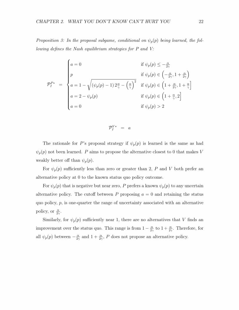
Proposition 3: In the proposal subgame, conditional on p(p) being learned, the fol-
lowing defines the Nash equilibrium strategies for P and V:
PP⇤I =
8>>>>>>>>>>>><
>>>>>>>>>>>>:
a = 0 if p(p) � ↵2�
p if p(p) 2⇣� ↵
2� , 1 +↵2�
⌘
a = 1�r
( p(p)� 1) 2
↵��⇣↵�
⌘2if p(p) 2
⇣1 +
↵2� , 1 +
↵�
i
a = 2� p(p) if p(p) 2⇣1 +
↵�, 2i
a = 0 if p(p) > 2
PV ⇤I = a
The rationale for P ’s proposal strategy if p(p) is learned is the same as had
p(p) not been learned. P aims to propose the alternative closest to 0 that makes V
weakly better off than p(p).
For p(p) sufficiently less than zero or greater than 2, P and V both prefer an
alternative policy at 0 to the known status quo policy outcome.
For p(p) that is negative but near zero, P prefers a known p(p) to any uncertain
alternative policy. The cutoff between P proposing a = 0 and retaining the status
quo policy, p, is one-quarter the range of uncertainty associated with an alternative
policy, or ↵2� .
Similarly, for p(p) sufficiently near 1, there are no alternatives that V finds an
improvement over the status quo. This range is from 1� ↵2� to 1+
↵2� . Therefore, for
all p(p) between � ↵2� and 1 +
↵2� , P does not propose an alternative policy.

CHAPTER 2. WHAT YOU DON’T KNOW CAN’T HURT YOU 23
Finally, for p(p) 2⇣1 +
↵2� , 2
⌘, P proposes the alternative for which V is indif-
ferent between retaining the status quo and accepting a.
Now, I examine the equilibrium behavior for P and V in the learning subgame,
conditional on the best responses in the proposal subgame.
Proposition 4: In the learning subgame, the following defines the Nash equlibrium
strategies for P and V.
LP⇤=
8><
>:
L if Eup(LP= L) � Eup(LP
= ¬L)
¬L otherwise
LV ⇤=
8>>>>><
>>>>>:
A if p �↵� ↵2�
¬A if p 2⇣�↵� ↵
2� ,↵2� � ↵
⌘
A otherwise
In the learning subgame, the equilibrium behavior for V is more straightforward
than for P .
In order to demonstrate the values of p for which V will veto a proposal to
learn p(p), I partition R into six segments, Pi, where i 2 {1, 2, 3, 4, 5, 6}. P1 =
(�1,�↵� ↵2� ], P2 = (�↵� ↵
2� , 0], P3 = (0, 2� ↵], P4 = (2� ↵, 2], P5 = (2, 2 + ↵],
and P6 = (2 + ↵,1).
For p 2 P1, for all possible values of p(p), P will propose a = 0 if p(p) is
learned. If p(p) is not learned, then P will propose a = 0 as well. Therefore, V is
indifferent between learning p(p) and not. As a result, V will accept a proposal to

CHAPTER 2. WHAT YOU DON’T KNOW CAN’T HURT YOU 24
learn p(p).
For p 2 P6, the same holds. For all possible values of p(p), P will propose a = 0
if p(p) is learned. If p(p) is not learned, then P will propose a = 0 as well.
For p 2 P2, if p(p) is not learned, then P will propose a = 0, V will accept,
and Euv = �1. Therefore, by learning p(p), V trades off the possibility that
p(p) 2 (� ↵2� , 0), in which case PP⇤
I is p < 0 and Euv < �1 against the possibility
that p(p) � 0, PP⇤I is p � 0, and Euv � �1. For p 2 (�↵� ↵
2� ,↵2� �↵), Pr( p(p) 2
(� ↵2� , 0)) > Pr( p(p) > 0) and V prefers not to learn p(p). For p 2 [
↵2� � ↵, 0], the
opposite is true and V prefers to learn p(p).
For p 2 P3, if p(p) is learned and P proposes an alternative, then V is indifferent
between the alternative and p(p). Similarly, if p(p) is not learned and P proposes
an alternative, V is made exactly as well off as if the status quo policy were to
remain. Therefore, V is indifferent between learning p(p) and not.
For p 2 P4, if p(p) is not learned, then P will propose an alternative that makes
V indifferent between accepting the alternative and retaining p. In contrast, if p(p)
is revealed to be greater than 2, P will propose a = 0, which makes V strictly better
off than p(p). Therefore, V prefers that p(p) be learned.
For p 2 P5, if p(p) is not learned, P will propose a = 0 and Euv(a) = �1. If
p(p) is revealed to be greater than 2, then P will also propose a = 0. But, if p(p)
is revealed to be less than 2, then P will propose a > 0 and Euv(a) > �1. As a
result, V is strictly better off if p(p) is learned.
P ’s decision whether or not to learn is considerably more involved. Implicitly, if
the expected utility from learning exceeds the expected utility from not learning, P
will propose to learn p(p). I demonstrate the equilibrium behavior for P through a
series of numerical examples in order to generate intuition for the conditions under
CHAPTER 2. WHAT YOU DON’T KNOW CAN’T HURT YOU 25
which not learning dominates learning and vice versa. The first two examples illus-
trate cases where internal politics create incentives for the proposer not to learn. The
third demonstrates how political considerations can make learning more desirable,
rather than less.
Example 1: Price-setting in a Manufacturing Firm
Background
Zbaracki and Bergen (2010) describe the internal politics of price-setting in a
manufacturing firm that sells products to warehouse distributors. They emphasize
the conflict between the marketing team and the sales team. The organization’s
goals included increasing market share and maximizing profit margins. Of these two
goals, the marketing team placed greater emphasis on the market share goal and
the sales team placed greater emphasis on the profit margin goal. These emphases
reflected the roles of each team in the company. Marketers were in charge of setting
pricing strategies that would enlarge the company’s client base. Members of the sales
team were tasked with developing long-term relationships with distributors, which
entailed significant discretion over discounting.
The disagreement over organizational outcomes created conflict over pricing strate-
gies. The marketing team desired lower prices across the board and less individual
discretion for the sales team. The sales team preferred higher prices and greater
discretion to discount. The marketing team justified their position by arguing that
prospective customers paid significant attention to list prices and that there was no
evidence that selective discounting increased revenue for the company. The sales
team believed that large customers did not take list prices seriously. Lower prices
merely constrained the company’s ability to price discriminate.
The conflict remained latent until the firm’s management decided to make a large
CHAPTER 2. WHAT YOU DON’T KNOW CAN’T HURT YOU 26
capital investment and to purchase a product line from a close competitor, generating
a sizable decline in production costs. The organizational change had a direct impact
on the firm’s existing pricing policy. If list prices were kept at the same levels, then
the sales team would have even more discretion than before. However, the marketing
team had institutional control over the published price lists. Marketing viewed the
decreased production costs as an opportunity to slash prices across the board.
Political conflict erupted between the marketing team and the sales team. Mar-
keting criticized sales for being “champions of high price” (Zbaracki and Bergen,
2010, p. 965). Sales responded that marketing had “very minimal experience in this
industry” and titled the MBA-laden pricing team “mahogany row” (Zbaracki and
Bergen, 2010, p. 965). According to one analyst, meetings between marketing and
sales to negotiate new pricing policies became so contentious that they approached
physical violence.
Notwithstanding the overt disagreement over organizational strategy, the mar-
keting team made no serious attempt to collect information or to model alternative
pricing schemes. Marketing admitted that they could not predict customer response
to a large cut in prices. Interestingly, however, they also did very little to collect in-
formation about the status quo pricing policy. They refused to incorporate the data
on differential pricing across market regions and product lines compiled by the sales
team into their pricing simulations. As the sales team lacked the information and
expertise to develop pricing simulations on their own, the political conflict erupted
in the absence of any hard data.
In the end, firm executives agreed to the recommendations of the marketing team
for the newer, high volume products, but made a specific exception for older products
in order to make the price changes revenue neutral. The director of sales acknowl-
edged that his team had lost in this political conflict: “You’ve got to move on. You
CHAPTER 2. WHAT YOU DON’T KNOW CAN’T HURT YOU 27
can’t keep fighting it. It is pointless. You have to move on and make it work”
(Zbaracki and Bergen, 2010, p. 966).
Strategic Analysis
I illustrate how it could be in the best interests of the marketing team to refuse
to collect information on the existing pricing scheme.
Define the outcome space by the relative importance of market share and profit
margins, where high market share and low profit margins map to low values in R.
Define preferences over policies by their expected outcomes, where low values indicate
lower prices and high values indicate more discretion.
Let the marketing team be P , which is consistent with marketing’s control over
the price lists and their ability to collect and analyze market data. Let sales be V .
Let p =
54 , indicating that the status quo policy (following the firm’s investment)
was more heavily weighted towards discretion than what was seen as optimal from the
perspectives of both marketing and sales. However, the status quo is substantially
less desirable from the perspective of the marketing team.
Let ↵ =
14 and � = 1, indicating a moderate level of uncertainty about the
mapping from the status quo policy to the status quo outcome. Because the status
quo policy was implemented prior to a significant organizational change, learning
p(p) provides no additional information about the mapping between a proposed
alternative and the associated policy outcome. Note that the sales team, V , will
accept a proposal from the marketing team, P , to learn p(p) (LV ⇤= A).
The strategic analysis involves calculating the expected utility for P if p(p) is
learned and if p(p) is not learned:
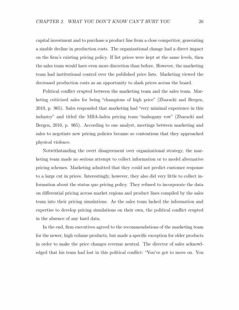
If the marketing team does not propose to learn (LP= ¬L), then the best
alternative proposal is 34 (PP⇤
¬L is a =
34), which is the nearest proposal to their ideal
CHAPTER 2. WHAT YOU DON’T KNOW CAN’T HURT YOU 28
outcome, 0, that makes the sales team just as well off. Because the range of outcomes
associated with the policy are distributed uniformly from 12 to 1, the expected utility
for the marketing team is �34 (Eup(LP
= ¬L) = �34). Note that for ease of notation,
I will denote Eup(LP= ¬L) and Eup(LP
= L) as Eup(¬L) and Eup(L).
The game outcome if the marketing team does not propose to learn (LP= ¬L)
is illustrated in Figure 2.1.
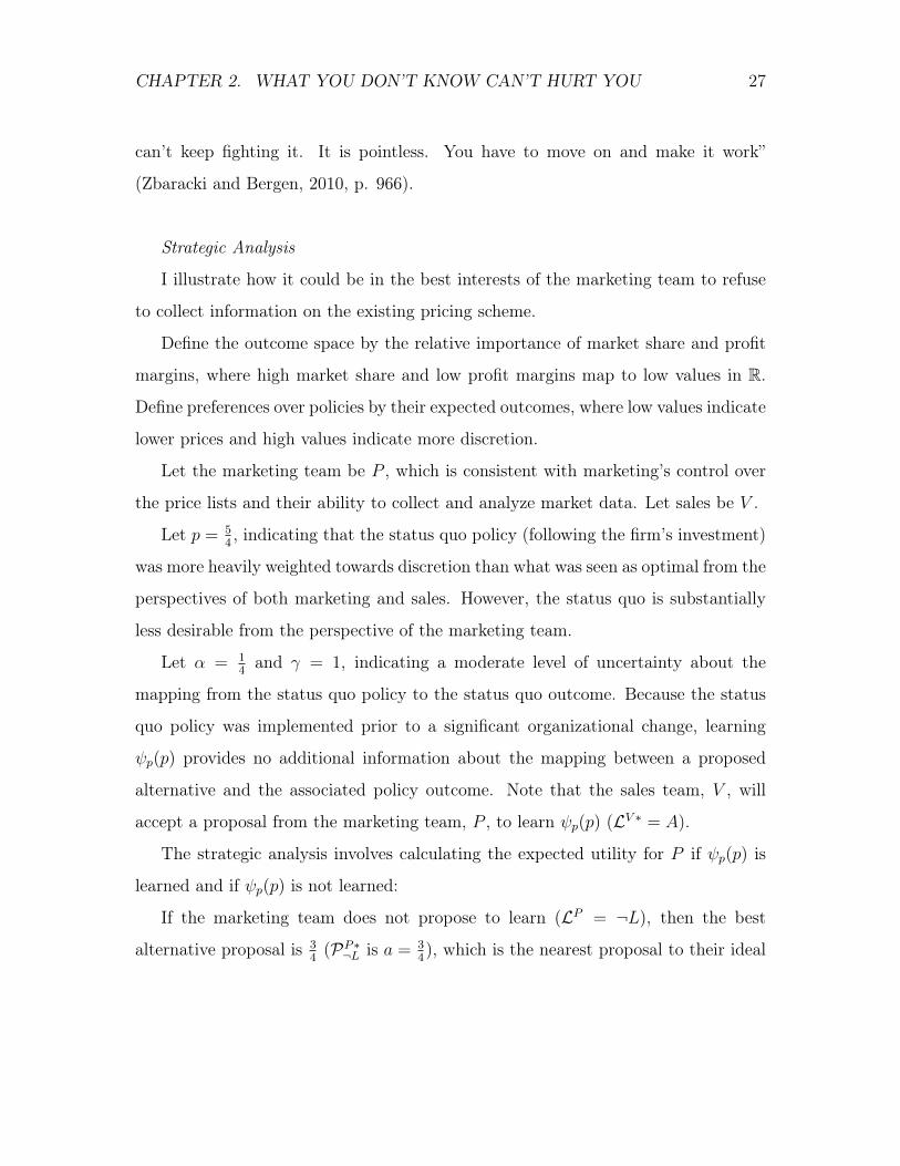
If the marketing team proposes to learn (LP= L), the sales team agrees (LV
=
L), and the organization learns that the status quo policy outcome, p(p), is between
1 and 98 , there is no alternative that the marketing team, P , can propose that makes
the sales team, V , better off. As a result, the marketing team does not propose an
alternative (PP⇤L = p). The probability that the status quo policy outcome lies in
this range is 14 ((Pr( p(p) <
98) =
14). The expected utility for the marketing team,
P , given that p(p) lies in this range is �1716 .
The game outcome if the marketing team proposes to learn (LP= L) and p(p) =
1716 is illustrated in Figure 2.2.
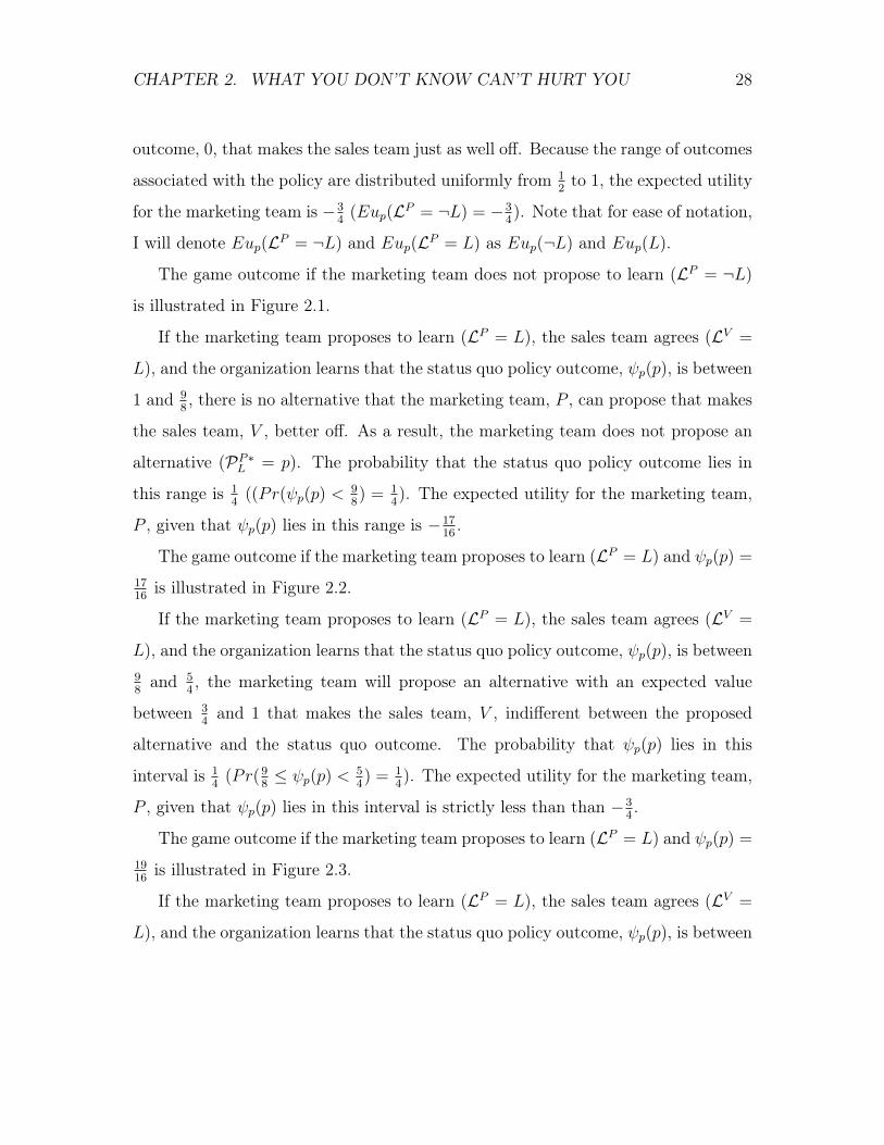
If the marketing team proposes to learn (LP= L), the sales team agrees (LV
=
L), and the organization learns that the status quo policy outcome, p(p), is between98 and 5
4 , the marketing team will propose an alternative with an expected value
between 34 and 1 that makes the sales team, V , indifferent between the proposed
alternative and the status quo outcome. The probability that p(p) lies in this
interval is 14 (Pr(98 p(p) <
54) =
14). The expected utility for the marketing team,
P , given that p(p) lies in this interval is strictly less than than �34 .
The game outcome if the marketing team proposes to learn (LP= L) and p(p) =
1916 is illustrated in Figure 2.3.
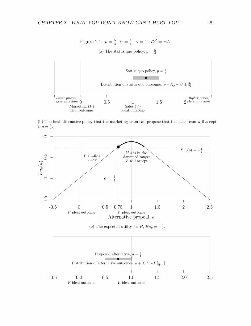
If the marketing team proposes to learn (LP= L), the sales team agrees (LV
=
L), and the organization learns that the status quo policy outcome, p(p), is between
CHAPTER 2. WHAT YOU DON’T KNOW CAN’T HURT YOU 29
Figure 2.1: p =
54 . ↵ =
14 . � = 1. LP
= ¬L.
(a) The status quo policy, p = 54 .
0 0.5 1 1.5 2Lower prices/Less discretion
Higher prices/More discretion
Marketing (P )ideal outcome
Sales (V )ideal outcome
Status quo policy, p =
54
Distribution of status quo outcomes, p+Xp ⇠ U [1, 32 ]
(b) The best alternative policy that the marketing team can propose that the sales team will acceptis a = 3
4 .
Alternative propoal, a
NA
Euv(a)
-0.5 0 0.5 0.75 1 1.5 2 2.5
-1.5
-1-0
.50
P ideal outcome V ideal outcome
V ’s utilitycurve
Euv(p) = �14If a is in the
darkened range:V will accept
a =
34
(c) The expected utility for P , Eup = � 34 .
P ideal outcome V ideal outcome
Proposed alternative, a =
34
Distribution of alternative outcomes, a+X¬Ia ⇠ U [
12 , 1]
-0.5 0.0 0.5 1.0 1.5 2.0 2.5
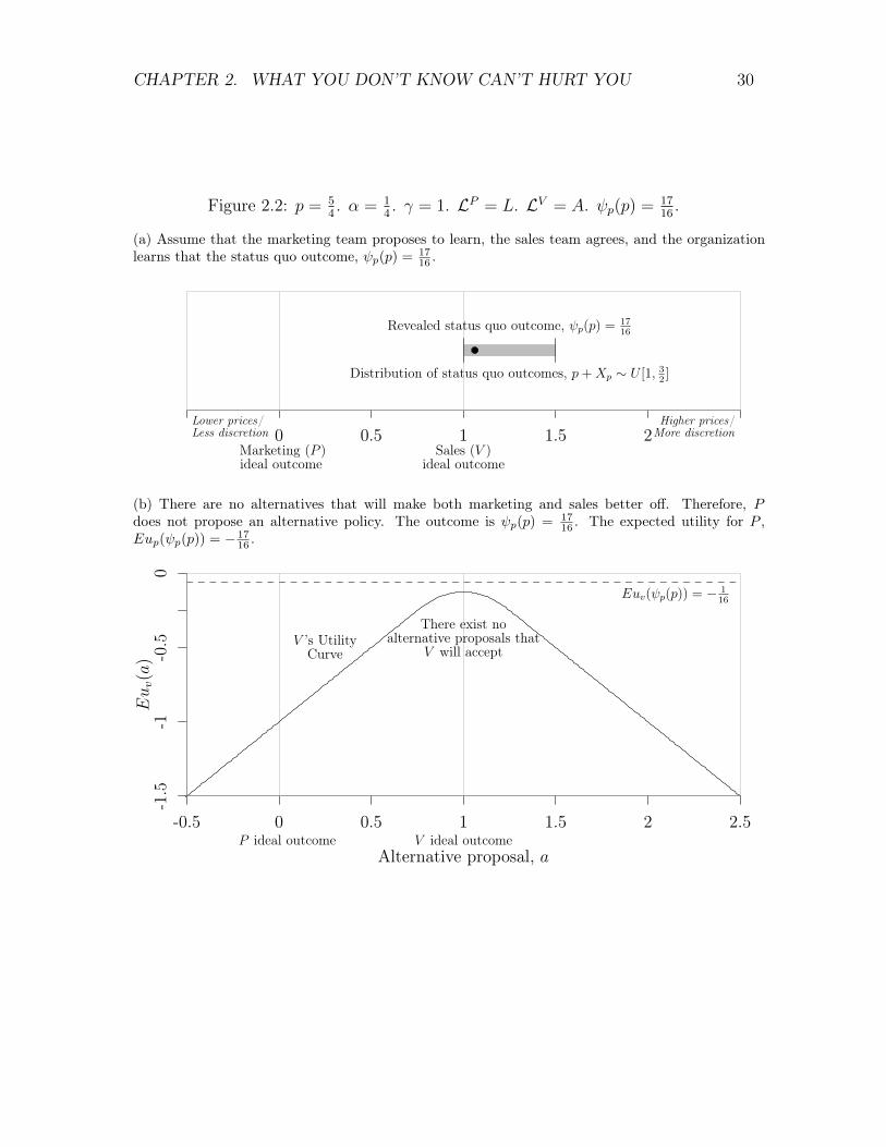
CHAPTER 2. WHAT YOU DON’T KNOW CAN’T HURT YOU 30
Figure 2.2: p =
54 . ↵ =
14 . � = 1. LP
= L. LV= A. p(p) =
1716 .
(a) Assume that the marketing team proposes to learn, the sales team agrees, and the organizationlearns that the status quo outcome, p(p) =
1716 .
0 0.5 1 1.5 2Lower prices/Less discretion
Higher prices/More discretion
Marketing (P )ideal outcome
Sales (V )ideal outcome
Revealed status quo outcome, p(p) =1716
Distribution of status quo outcomes, p+Xp ⇠ U [1, 32 ]
(b) There are no alternatives that will make both marketing and sales better off. Therefore, Pdoes not propose an alternative policy. The outcome is p(p) = 17
16 . The expected utility for P ,Eup( p(p)) = � 17
16 .
Alternative proposal, a
NA
Euv(a)
-0.5 0 0.5 1 1.5 2 2.5
-1.5
-1-0
.50
P ideal outcome V ideal outcome
V ’s UtilityCurve
Euv( p(p)) = � 116
There exist noalternative proposals that
V will accept

CHAPTER 2. WHAT YOU DON’T KNOW CAN’T HURT YOU 31
Figure 2.3: p =
54 . ↵ =
14 . � = 1. LP
= L. LV= A. p(p) =
1916 .
(a) Assume that the marketing team proposes to learn, the sales team agrees, and the organizationlearns that the status quo outcome, p(p) =
1916 .
0 0.5 1 1.5 2Lower prices/Less discretion
Higher prices/More discretion
Marketing (P )ideal outcome
Sales (V )ideal outcome
Revealed status quo outcome, p(p) =1916
Distribution of status quo outcomes, p+Xp ⇠ U [1, 32 ]
(b) The best alternative policy that the marketing team can propose that the sales team will acceptis a = 0.82.
Alternative proposal, a
NA
Euv(a)
-0.5 0 0.5 0.82 1 1.5 2 2.5
-1.5
-1-0
.50
P ideal outcome V ideal outcome
V ’s UtilityCurve
EUv( p(p)) = � 316
If a is inthe darkened range:
V will accept
a = 0.82
(c) The expected utility for P , Eup = �0.82.
P ideal outcome V ideal outcome
Proposed alternative, a = 0.82
Distribution of alternative outcomes, a+XIa ⇠ U [0.57, 1.07]
-0.5 0.0 0.5 1.0 1.5 2.0 2.5

CHAPTER 2. WHAT YOU DON’T KNOW CAN’T HURT YOU 32
54 and 3
2 , then the marketing team will propose an alternative policy with an expected
value between 12 and 3
4 such that the sales team is indifferent between the proposed
alternative and the status quo outcome. The probability that p(p) lies in this
interval is 12 (Pr( p(p) � 5
4) =
12). The expected utility for the marketing team
given that p(p) lies in this interval is �58 .
The game outcome if the marketing team proposes to learn (LP= L) and p(p) =
118 is illustrated in Figure 2.4.
If the marketing team proposes to learn (LP= L), the marketing team has a 25
percent chance of expected utility of �1716 , a 25 percent chance of expected utility less
than �34 , and a 50 percent chance of expected utility of �5
8 . The expected utility for
the marketing team if they propose to learn, therefore, is lower than the expected
utility if they do not (Eup(L) < Eup(¬L)).
Eup(L) = Pr( p(p) <9
8)(Eup| p(p) <
9
8) +
Pr(9
8 p(p) <
5
4)(Eup|
9
8 p(p) <
5
4) + Pr( p(p) �
5
4)(Eup| p(p) �
5
4)
Eup(L) <1
4·�17
16+
1
4·�3
4+
1
2·�5
8
Eup(L) < �3
4
Eup(¬L) = �3
4
Eup(¬L) > Eup(L)
Thus, the marketing team chooses not to propose to learn (LP⇤= ¬L).
Conclusion
Because learning about the uncertain status quo policy increases the likelihood
that the sales team would refuse any potential proposed alternative, the marketing
team prefers to make a proposal without learning the mapping of the status quo
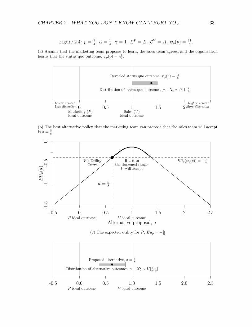
CHAPTER 2. WHAT YOU DON’T KNOW CAN’T HURT YOU 33
Figure 2.4: p =
54 . ↵ =
14 . � = 1. LP
= L. LV= A. p(p) =
118 .
(a) Assume that the marketing team proposes to learn, the sales team agrees, and the organizationlearns that the status quo outcome, p(p) =
118 .
0 0.5 1 1.5 2Lower prices/Less discretion
Higher prices/More discretion
Marketing (P )ideal outcome
Sales (V )ideal outcome
Revealed status quo outcome, p(p) =118
Distribution of status quo outcomes, p+Xp ⇠ U [1, 32 ]
(b) The best alternative policy that the marketing team can propose that the sales team will acceptis a = 5
8 .
Alternative proposal, a
NA
EUv(a)
-0.5 0 0.5 1 1.5 2 2.5
-1.5
-1-0
.50
P ideal outcome V ideal outcome
V ’s UtilityCurve
EUv( p(p)) = �38
If a is inthe darkened range:
V will accept
a =
58
(c) The expected utility for P , Eup = � 58
P ideal outcome V ideal outcome
Proposed alternative, a =
58
Distribution of alternative outcomes, a+XIa ⇠ U [
38 ,
78 ]
-0.5 0.0 0.5 1.0 1.5 2.0 2.5
CHAPTER 2. WHAT YOU DON’T KNOW CAN’T HURT YOU 34
policy to its associated outcome.
Example 2: U.S. Congressional Investigations Following the Financial Cri-
sis of 2008
Background
In the aftermath of the 2008 financial crisis and, in particular, following the emer-
gency passage of legislation approving the Troubled Asset Relief Program, Democrat
and Republican legislators in the U.S. Congress agreed that the American financial
regulatory regime was badly broken. Traditionally, Democrats in Congress supported
a more stable financial system at the cost of sacrificed economic growth. Republi-
cans, in contrast, were willing to risk greater financial instability for faster economic
growth. These disagreements over economic values tended to play out in negotia-
tions over financial regulatory policy. Democrats supported more stringent banking
regulation. Republicans tended to favor deregulation.
After the financial crisis, however, Democrats and Republicans agreed that the
needle had swung too far towards deregulation. The debate was over how much
additional regulation was necessary. Congressional Democrats supported replacing
the existing regulatory apparatus with a regime similar to the one in place following
the Great Depression. Congressional Republicans supported more targeted reforms.
It is common for the U.S. legislature to establish investigatory commissions when
national emergencies occur that warrant policy intervention. Investigatory commis-
sions of this type were created to great fanfare following the Great Depression, the
Challenger Disaster, and the terrorist attack on the World Trade Center. The in-
vestigative reports published by these commissions were influential in directing the
subsequent policy debate. Even today, the Pecora Commission, the Rogers Commis-
sion, and the 9/11 Commission remain a part of public discourse.
CHAPTER 2. WHAT YOU DON’T KNOW CAN’T HURT YOU 35
However, Democrats in the Congress were unenthusiastic about creating a com-
mission following the financial crisis. Chairman of the House Financial Services Com-
mittee Barney Frank called proposals to form an investigatory commission “a silly
idea whose time has come” (Kaiser, 2013). Unable to keep a commission from being
created, Frank instead convinced congressional leadership in the House of Represen-
tatives to stipulate that the commission’s findings be published after the financial
reform effort was complete.
Sweeping financial reforms were signed by the President on July 21, 2010. Major
changes included the creation of new regulatory agencies, significant expansion of
existing regulatory authority, and the re-introduction of restrictions on investment
behavior that had been slowly eroded through deregulation.
The results of the commission’s investigation were published six months later.
Strategic Analysis
I demonstrate one reason why Congressional Democrats were opposed to the
creation of an investigatory commission.
Define the outcome space by the relative importance of economic stability and
economic growth, where high stability and low growth map to low values in R. Define
preferences over policies by their expected outcomes, where low values indicate more
market regulation and high values indicate less market regulation.
Let Democrats be P , which is consistent with the partisan control of the Congress
and the Executive when the commission was proposed. Let Republicans be V .
Let p = 1.9, indicating that the status quo policy (following the financial crisis)
was more heavily weighted towards instability than what was seen as optimal from
the perspectives of both Democrats and Republicans.
Let ↵ =
12 and � =
54 . There is high uncertainty about the mapping between
CHAPTER 2. WHAT YOU DON’T KNOW CAN’T HURT YOU 36
the status quo policy and status quo outcome, although there is agreement that all
possible status quo outcomes are associated with too little regulation. Learning about
the mapping between the status quo policy and policy outcome does provide some
additional information about the distribution of outcomes resulting from proposed
alternatives. This differs from the previous example, in which learning about the
mapping from status quo policy to status quo outcome did not decrease the range of
possible outcomes resulting from proposed alternatives.
LV ⇤= A, indicating that V will accept a proposal to learn p(p).
If LP= ¬L, then PP ⇤
¬L is a = 0.1, which is the nearest point to 0 which makes V
just as well off. Eup(¬L) = �0.26.
If LP= L and p(p) 2 [1
25 , 1
35), P will propose a = 2 � p(p). The probability
that p(p) 2 [1
25 , 1
35) is 1
5 . The expected utility for P given p(p) 2 [1
25 , 1
35) is �1
2 .
If LP= L and p(p) 2 [1
35 , 2), P will propose a 2 (0, 25) . The probability that
p(p) 2 [1
35 , 2) is 2
5 . The expected utility for P given p(p) 2 [1
35 , 2) is strictly less
than �15 .
If LP= L and p(p) 2 [2, 22
5 ]. P will propose a = 0. The probability that
p(p) 2 [2, 225 ] is 2
5 . The expected utility for P given p(p) 2 [2, 225 ] is �1
5 .
As a result, if LP= L, P has a 20 percent chance of expected utility of �1
2 , a 40
percent chance of expected utility of �15 , and a 40 percent chance of expected utility
of strictly less than �15 , which is less than Eup(¬L) = �0.26.
Thus, LP⇤= ¬L.
Conclusion
Congressional Democrats would do fairly well without learning, because the status
quo policy is thought to be so extreme. If they investigate, Congressional Republicans
could learn that the current regulatory system was stronger than had previously been
CHAPTER 2. WHAT YOU DON’T KNOW CAN’T HURT YOU 37
thought, in which case Democrats would be unable to get as desirable a new policy
accepted by Republicans. Although, if they investigate, Congressional Democrats
could learn that the current regime was even less regulated than legislators previ-
ously thought, the political value of this information is bounded by the Democrats’
ideal outcome.
Example 3: Drug Testing, Major League Baseball, and the Players’ Union
Background
The late 1990s were a boon to Major League Baseball. The assaults on Roger
Maris’ storied home run record by sluggers Mark McGwire, Ken Griffey, Jr., Sammy
Sosa, and Barry Bonds brought fans back to baseball after a nasty labor dispute
canceled the 1994 World Series. However, the power surge also stimulated suspicion
among baseball fans about the possibility of widespread performance-enhancing drug
use. Following a series of investigations into specific players and even some high
profile admissions of guilt, the Office of the Commissioner came to believe that
steroid use was hurting the long-term popularity of the sport.
The Major League Baseball Players Association agreed that steroid use was a
problem, but was deeply uncomfortable with subjecting its members to the steroid
testing regime proposed by the owners. The union was concerned that the owners
would use steroid tests as a tool to discriminate against disfavored players, that
violators could be open to federal prosecution, and that the testing regime could be
a first step towards more draconian oversight over the private lives of players. The
union was willing to make steroid testing a part of the collective bargaining process,
but expected concessions from ownership in order to accept widespread randomized
testing and stiff penalties for violators.
In 2006, Major League Baseball commissioned a report on the prevalence of
CHAPTER 2. WHAT YOU DON’T KNOW CAN’T HURT YOU 38
steroid use in baseball, which was conducted by former U.S. Senator George Mitchell.
The report, which was completed in the fall of 2007, found conclusive evidence of
performance-enhancing drug use by 89 current and former players (Mitchell, 2007).
Included in the report were also interviews with current and former players and
coaches that insinuated that the problem of performance-enhancing drugs was far
more widespread than had been expected.
The resulting change in player perceptions about the prevalence of performance-
enhancing drugs in baseball combined with the bad public optics of appearing to be
in favor of illegal drugs have led the union to take a more conciliatory stance towards
increased testing. In the 2011 negotiations between the commissioner’s office and the
union, the players accepted significantly more stringent testing standards, including
agreeing to the collection of blood samples to test for human growth hormone. In
2013, the players’ union also agreed to increased penalties for players caught using
performance-enhancing drugs, random blood tests, and substantially increased su-
pervision for past offenders.
Strategic Analysis
I illustrate how the decision to commission a report on steroids in baseball helped
the commissioner’s office in negotiations with the Major League Baseball Players
Association.
Define the outcome space by the relative importance of clean players and per-
sonal privacy, where clean players and low privacy map to low values in R. Define
preferences over policies by their expected outcomes, where low values indicate more
drug testing and high values indicate less drug testing.
Let the Office of the Commissioner be P , which is consistent with power that
owners have over the players and the considerably greater resources at the disposal

CHAPTER 2. WHAT YOU DON’T KNOW CAN’T HURT YOU 39
of the commissioner than the head of the players’ association. Let the union be V .
Let p = 1, indicating that the status quo policy is optimal from the perspective
of the union, but undesirable from the perspective of the owners.
Let ↵ =
310 and � = 1, indicating a moderate level of uncertainty about the
prevalence of the use of steroids in the current regime. Also, as there is no formal
drug testing policy in place, learning the current rate of steroid usage does not reduce
the uncertainty surrounding an alternative performance-enhancing drug policy.
LV ⇤= A, indicating that V will accept a proposal to learn p(p).
If LP= ¬L, then PP⇤
¬L = p, because there are no alternative policies than can
make the union better off than the status quo. Eup(¬L) = �1.
If LP= L and p(p) 2 [1
320 , 1
310 ], P will propose a 2 [
710 , 1]. The probability that
p(p) 2 [1
320 , 1
310 ] is 1
4 . The expected utility for P given p(p) 2 [1
320 , 1
310 ] is strictly
greater than �1.
If LP= L and p 2 [
710 , 1
320), P will not propose an alternative. The probability
that p(p) 2 [
710 , 1
320) is 3
4 . The expected utility for P given p(p) 2 [
710 , 1
320) is �1.
As a result, if LP= L, P has a 75 percent chance of expected utility of �1, but
a 25 percent chance of expected utility greater than �1.
Thus, LP⇤= L.
Conclusion
Absent the report, players would believe that the modest amount of performance-
enhancing drugs in baseball outstripped the necessary sacrifice of personal privacy
associated with more stringent controls. If the report found there was less drug usage
than expected, then the Commissioner’s office would be no worse off. In contrast, if
the report found greater drug usage than expected, then the players would be more
willing to agree to a tighter drug testing regime.

CHAPTER 2. WHAT YOU DON’T KNOW CAN’T HURT YOU 40
The Learning Decision
These three examples illustrate how conflicting preferences can complicate incen-
tives for organizational learning. I now generalize from the examples and explore
the organization’s decision whether or not to learn for a range of parameter values.
The analysis highlights a few important insights about equilibrium behavior in the
model. First, the strength of the incentives both to learn p(p) and not to learn
p(p) grow with ↵. Second, as � increases, the incentives to learn for both P and
V increase as well. However, even for high values of �, there remain values of p for
which P does not propose to learn p(p) and for which V vetoes a proposal to learn
p(p). Finally, for all values of p such that the organization does not learn p(p), p
is either less than 0 or greater than 1. Therefore, the organization only chooses not
to learn p(p) when the existing policy is undesirable for both P and V .
Figures 2.5, 2.6, and 2.7 illustrate the expected utility functions for the proposer
and the veto conditional on p and whether p(p) is learned for ↵ 2 { 110 ,
14 ,
12} and
� = 1 (on the left) and the difference between the utility functions if p(p) is learned
and if p(p) is not learned (on the right). The top left panels demonstrate the
proposer’s expected utility if p(p) is learned and the proposer’s expected utility
if p(p) is not learned. The bottom left panels demonstrate the veto’s expected
utility if p(p) is learned and the veto’s expected utility if p(p) is not learned. The
right panels illustrates the differences between the two expected utilities for P and
V . Higher values on the right panel indicate a larger benefit to learning relative to
ignorance.
Figure 2.5 compares Eup and Euv when p(p) is learned and when p(p) is not
learned for ↵ =
110 and � = 1. Eup,v(I) represents the expected utility for P or V if
p(p) is learned. Eup,v(¬I) represents the expected utility for P or V if p(p) is not

CHAPTER 2. WHAT YOU DON’T KNOW CAN’T HURT YOU 41
Figure 2.5: ↵ =
110 . � = 1.
Eup
-1 0 1 2 3
-1.0
-0.6
-0.2
Eup(I)Eup(¬I)
Euv
Status Quo Policy, p
-1 0 1 2 3
-1.0
-0.6
-0.2 Euv(I)
Euv(¬I)
P idealoutcome
V idealoutcome
Status Quo Policy, p
-1 0 1 2 3
-0.1
0.0
0.1
0.2
Exp
ecte
dU
tility
Gai
nfr
omLe
arni
ng
Eup(I) - Eup(¬I)Euv(I) - Euv(¬I)
P idealoutcome
V idealoutcome
Status Quo Policy, p
Comparing Eup,v(I) to Eup,v(¬I) Eup,v(I)� Eup,v(¬I)
learned.
Figure 2.5 indicates that when the level of uncertainty in the mapping from
policies to outcomes is small, the strategic choice to learn p(p) is less important.
However, even with low uncertainty, for both P and V the incentives to keep the
organization from learning p(p) are largest when p is believed to be undesirable.
Figures 2.6 and 2.7 demonstrate how these results change as the level of uncer-
tainty increases. Figure 2.6 compares Eup,v(I) and Eup,v(¬I) when ↵ =
14 and � = 1.
Figure 2.7 compares Eup,v(I) and Eup,v(¬I) when ↵ =
12 and � = 1.
There are three major differences between Figures 2.5, 2.6, and 2.7. As uncer-
tainty increases, the size of the expected utility difference between learning and not
learning increases for both P and V . Also, both the range of values for which learn-
ing dominates not learning and the range of values for which not learning dominates
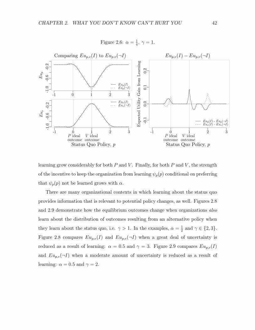
CHAPTER 2. WHAT YOU DON’T KNOW CAN’T HURT YOU 42
Figure 2.6: ↵ =
14 . � = 1.
Eup
-1 0 1 2 3
-1.0
-0.6
-0.2
Eup(I)Eup(¬I)
Euv
Status Quo Policy, p
-1 0 1 2 3
-1.0
-0.6
-0.2 Euv(I)
Euv(¬I)
P idealoutcome
V idealoutcome
Status Quo Policy, p
-1 0 1 2 3
-0.1
0.0
0.1
0.2
Exp
ecte
dU
tility
Gai
nfr
omLe
arni
ng
Eup(I) - Eup(¬I)Euv(I) - Euv(¬I)
P idealoutcome
V idealoutcome
Status Quo Policy, p
Comparing Eup,v(I) to Eup,v(¬I) Eup,v(I)� Eup,v(¬I)
learning grow considerably for both P and V . Finally, for both P and V , the strength
of the incentive to keep the organization from learning p(p) conditional on preferring
that p(p) not be learned grows with ↵.
There are many organizational contexts in which learning about the status quo
provides information that is relevant to potential policy changes, as well. Figures 2.8
and 2.9 demonstrate how the equilibrium outcomes change when organizations also
learn about the distribution of outcomes resulting from an alternative policy when
they learn about the status quo, i.e. � > 1. In the examples, ↵ =
12 and � 2 {2, 3}.
Figure 2.8 compares Eup,v(I) and Eup,v(¬I) when a great deal of uncertainty is
reduced as a result of learning: ↵ = 0.5 and � = 3. Figure 2.9 compares Eup,v(I)
and Eup,v(¬I) when a moderate amount of uncertainty is reduced as a result of
learning: ↵ = 0.5 and � = 2.
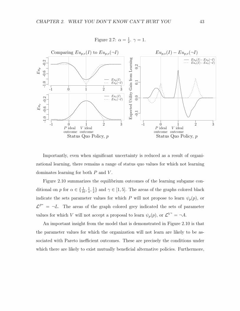
CHAPTER 2. WHAT YOU DON’T KNOW CAN’T HURT YOU 43
Figure 2.7: ↵ =
12 . � = 1.
Eup
-1 0 1 2 3
-1.0
-0.6
-0.2
Eup(I)Eup(¬I)
Euv
Status Quo Policy, p
-1 0 1 2 3
-1.0
-0.6
-0.2 Euv(I)
Euv(¬I)
P idealoutcome
V idealoutcome
Status Quo Policy, p
-1 0 1 2 3
-0.1
0.0
0.1
0.2
Exp
ecte
dU
tility
Gai
nfr
omLe
arni
ng Eup(I) - Eup(¬I)Euv(I) - Euv(¬I)
P idealoutcome
V idealoutcome
Status Quo Policy, p
Comparing Eup,v(I) to Eup,v(¬I) Eup,v(I)� Eup,v(¬I)
Importantly, even when significant uncertainty is reduced as a result of organi-
zational learning, there remains a range of status quo values for which not learning
dominates learning for both P and V .
Figure 2.10 summarizes the equilibrium outcomes of the learning subgame con-
ditional on p for ↵ 2 { 110 ,
14 ,
12} and � 2 [1, 5]. The areas of the graphs colored black
indicate the sets parameter values for which P will not propose to learn p(p), or
LP ⇤= ¬L. The areas of the graph colored grey indicated the sets of parameter
values for which V will not accept a proposal to learn p(p), or LV ⇤= ¬A.
An important insight from the model that is demonstrated in Figure 2.10 is that
the parameter values for which the organization will not learn are likely to be as-
sociated with Pareto inefficient outcomes. These are precisely the conditions under
which there are likely to exist mutually beneficial alternative policies. Furthermore,
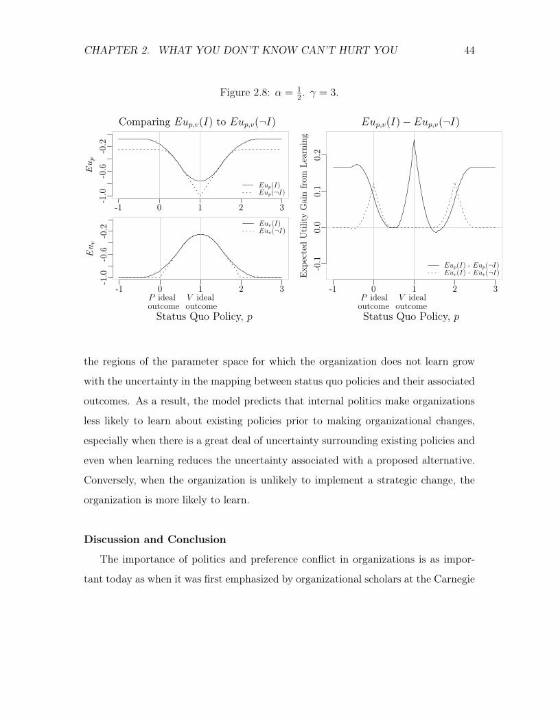
CHAPTER 2. WHAT YOU DON’T KNOW CAN’T HURT YOU 44
Figure 2.8: ↵ =
12 . � = 3.
Eup
-1 0 1 2 3
-1.0
-0.6
-0.2
Eup(I)Eup(¬I)
Euv
Status Quo Policy, p
-1 0 1 2 3
-1.0
-0.6
-0.2 Euv(I)
Euv(¬I)
P idealoutcome
V idealoutcome
Status Quo Policy, p
-1 0 1 2 3
-0.1
0.0
0.1
0.2
Exp
ecte
dU
tility
Gai
nfr
omLe
arni
ng
Eup(I) - Eup(¬I)Euv(I) - Euv(¬I)
P idealoutcome
V idealoutcome
Status Quo Policy, p
Comparing Eup,v(I) to Eup,v(¬I) Eup,v(I)� Eup,v(¬I)
the regions of the parameter space for which the organization does not learn grow
with the uncertainty in the mapping between status quo policies and their associated
outcomes. As a result, the model predicts that internal politics make organizations
less likely to learn about existing policies prior to making organizational changes,
especially when there is a great deal of uncertainty surrounding existing policies and
even when learning reduces the uncertainty associated with a proposed alternative.
Conversely, when the organization is unlikely to implement a strategic change, the
organization is more likely to learn.
Discussion and Conclusion
The importance of politics and preference conflict in organizations is as impor-
tant today as when it was first emphasized by organizational scholars at the Carnegie
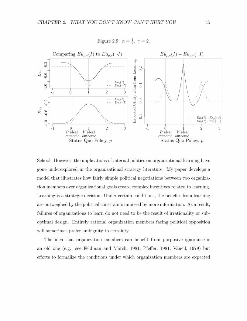
CHAPTER 2. WHAT YOU DON’T KNOW CAN’T HURT YOU 45
Figure 2.9: ↵ =
12 . � = 2.
Eup
-1 0 1 2 3
-1.0
-0.6
-0.2
Eup(I)Eup(¬I)
Euv
Status Quo Policy, p
-1 0 1 2 3
-1.0
-0.6
-0.2 Euv(I)
Euv(¬I)
P idealoutcome
V idealoutcome
Status Quo Policy, p
-1 0 1 2 3
-0.1
0.0
0.1
0.2
Exp
ecte
dU
tility
Gai
nfr
omLe
arni
ng
Eup(I) - Eup(¬I)Euv(I) - Euv(¬I)
P idealoutcome
V idealoutcome
Status Quo Policy, p
Comparing Eup,v(I) to Eup,v(¬I) Eup,v(I)� Eup,v(¬I)
School. However, the implications of internal politics on organizational learning have
gone underexplored in the organizational strategy literature. My paper develops a
model that illustrates how fairly simple political negotiations between two organiza-
tion members over organizational goals create complex incentives related to learning.
Learning is a strategic decision. Under certain conditions, the benefits from learning
are outweighed by the political constraints imposed by more information. As a result,
failures of organizations to learn do not need to be the result of irrationality or sub-
optimal design. Entirely rational organization members facing political opposition
will sometimes prefer ambiguity to certainty.
The idea that organization members can benefit from purposive ignorance is
an old one (e.g. see Feldman and March, 1981; Pfeffer, 1981; Vancil, 1979) but
efforts to formalize the conditions under which organization members are expected
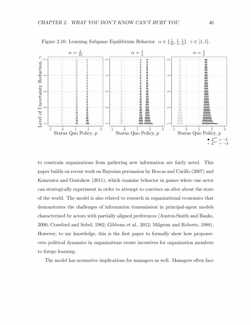
CHAPTER 2. WHAT YOU DON’T KNOW CAN’T HURT YOU 46
Figure 2.10: Learning Subgame Equilibrium Behavior. ↵ 2 { 110 ,
14 ,
12}. � 2 [1, 5].
-1 0 1 2 3
12
34
5
↵ =
110
Status Quo Policy, p-1 0 1 2 3
12
34
5
↵ =
14
Status Quo Policy, p-1 0 1 2 3
12
34
5
↵ =
12
Status Quo Policy, p
Leve
lofU
ncer
tain
tyR
educ
tion,�
LP ⇤= ¬L
LV ⇤= ¬A
to constrain organizations from gathering new information are fairly novel. This
paper builds on recent work on Bayesian persuasion by Brocas and Carillo (2007) and
Kamenica and Gentzkow (2011), which examine behavior in games where one actor
can strategically experiment in order to attempt to convince an alter about the state
of the world. The model is also related to research in organizational economics that
demonstrates the challenges of information transmission in principal-agent models
characterized by actors with partially aligned preferences (Austen-Smith and Banks,
2000; Crawford and Sobel, 1982; Gibbons et al., 2012; Milgrom and Roberts, 1988).
However, to my knowledge, this is the first paper to formally show how proposer-
veto political dynamics in organizations create incentives for organization members
to forego learning.
The model has normative implications for managers as well. Managers often face
CHAPTER 2. WHAT YOU DON’T KNOW CAN’T HURT YOU 47
steady institutional pressure to justify new proposals with objective data and analysis
(Feldman and March, 1981). Naïve managers see these requests for information as
a part of an organizational effort to achieve commonly held goals and, as a result,
always acquiesce. Strategic managers realize that requests for more information by
organization members are a part of a political process. As a result, strategic managers
may refuse to collect information. In fact, strategic managers will sometimes even
be willing to pay a personal cost to impede the capacity of political rivals to learn.
Lastly, the model helps organizational researchers better understand two frus-
trating observations about organizational learning and organizational change. One
reason why organizations frequently fail to learn about existing strategies or policies
prior to implementing organizational changes is because there are groups within or-
ganizations who fear that the results of such an investigation will disadvantage them
politically. These fears, however, do not exist when existing strategies are Pareto
efficient. Thus, organization members are likely to be willing to learn about existing
policies when it is unlikely that there is sufficient support in favor of an alternative to
replace the existing strategy. The ironic conclusion, therefore, is that organizations
will not learn when a policy change is likely to occur and will learn when a policy
change is unlikely to be enacted.
Chapter 3
Organizations Experimenting With
Managers Experimenting With
Strategies
Introduction
A hallmark of successful organizations is their ability to continually produce
fundamental innovations that fuel growth in the long term (Anderson and Tush-
man, 1990; O’Reilly and Tushman, 2013; Tushman and Anderson, 1986; Tushman
and O’Reilly, 1996; Utterback, 1994). However, despite the payoffs for organiza-
tions that sustain the type of wide-ranging exploration required to promote durable
competitive advantage, organizations consistently find it challenging to induce their
members to take big risks with uncertain payoffs. Due to inertial organizational rou-
tines, difficulties with cross-unit collaboration, political conflict, and managerial risk
aversion, innovation in organizations is often overly incremental (Cyert and March,
48
CHAPTER 3. ORGANIZATIONAL EXPERIMENTING WITH MANAGERS 49
1963; DiMaggio and Powell, 1983; Gibbons and Roberts, 2012; Hannan and Free-
man, 1984; Levitt and March, 1988; March, 1991; March and Shapira, 1987; Shapira,
1995). Managers seek smaller, exploitative improvements to existing products, ser-
vices, and technologies instead of the large, bold innovations that are required to
maintain long-term performance.
One way that organizations try to induce managers to overcome inertia, risk
aversion, and incrementalism is by encouraging managers to experiment offline. As
opposed to online search, in which organizations fully implement strategic changes
and then observe whether or not the changes worked, offline experimentation allows
organizations to observe the results of small-scale tests of alternative strategies prior
to committing to a new initiative. Clinical trials by drug companies, A/B testing
by internet search engines, and weapons prototypes in the defense industry are all
examples of offline experiments. By reducing the stakes associated with a failed
experiment, organizations attempt to induce members to take bigger risks. The
knowledge gleaned from offline experiments is then used to inform the strategies
that organizations choose to take online (Csaszar and Levinthal, 2016; Gavetti and
Levinthal, 2000; Kelley and Littman, 2001; Lippman and McCall, 1976; Pfeffer and
Sutton, 2006b).
However, experimenting offline fails to resolve a classic agency problem associated
with risky experimentation in organizations (Aghion and Jackson, 2014; Gibbons and
Roberts, 2012). Offline experiments not only offer managers the opportunity to test
alternative strategies, but also offer organizations the opportunity to evaluate the
competence of managers at their assigned task. It can be difficult for a firm to
distinguish between a good experimenter who had bad luck with an experiment and
a poorly matched or incompetent experimenter. For example, a graduate student in
the biological sciences whose dissertation research finds null results will often have a
CHAPTER 3. ORGANIZATIONAL EXPERIMENTING WITH MANAGERS 50
difficult time finding a post-doctoral research position, because prospective employers
cannot tell whether the student’s experimental work utilized proper research methods
or whether the experiments the student conducted were fundamentally flawed. As
a result, when a strategic manager faces with the choice between (1) designing an
offline experiment with a goal in mind that the organization finds desirable and
believes to be attainable and (2) designing an experiment with a targeted goal that
is undesirably incremental or impractically blue sky, the manager may prefer the
second. A failure to achieve an attainable goal reveals the manager as possibly
incompetent or poorly matched. Successfully reaching an incremental goal or failing
to achieve an unattainable one reveals less about a manager’s competence or fit.
Managers who seek to avoid revealing information about their quality do not nec-
essarily undertake experiments that are overly incremental from the perspective of
the organization. In fact, some of the same factors that lead managers to be overly
incremental when searching online can lead managers to be overzealous in their offline
search behavior. When pushed, managers will select goals that go far beyond what
can be successfully integrated by an organization in the hope of demonstrating their
capability to be innovative to superiors. Rather than coloring outside the lines, these
managers will color “on an entirely different page” (Kelley and Littman, 2001). IDEO
general manager Tom Kelley describes the “joyful failure” of the Enorme phone, a
product co-designed with an iconic Italian designer that sought to bring Italian de-
sign aesthetics together with Silicon Valley telephone engineering. The effort was
undoubtedly innovative: an example of the phone remains in the permanent collec-
tion of the Museum of Modern Art in New York. It was also an abject failure as a
consumer product. At $150 apiece at a time when customers could easily get a phone
for a few dollars, there was no consumer demand for the “playful cubist” telephone
(Kelley and Littman, 2001). These blue sky efforts are no better for organizations
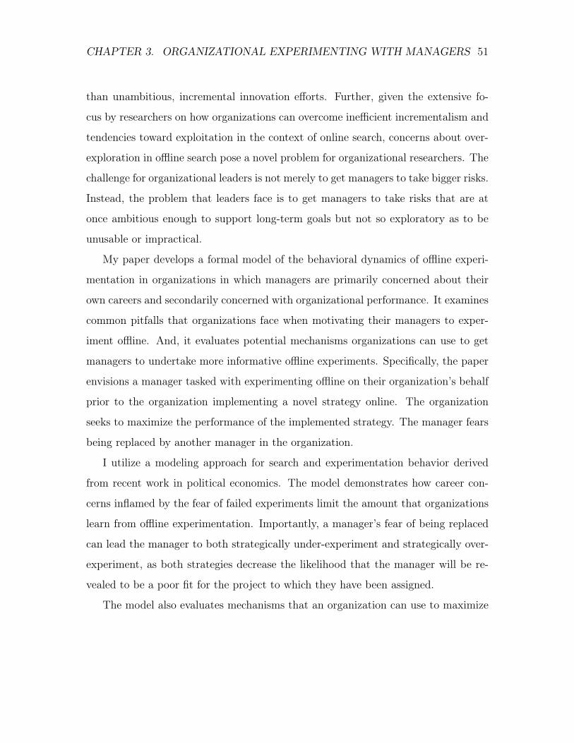
CHAPTER 3. ORGANIZATIONAL EXPERIMENTING WITH MANAGERS 51
than unambitious, incremental innovation efforts. Further, given the extensive fo-
cus by researchers on how organizations can overcome inefficient incrementalism and
tendencies toward exploitation in the context of online search, concerns about over-
exploration in offline search pose a novel problem for organizational researchers. The
challenge for organizational leaders is not merely to get managers to take bigger risks.
Instead, the problem that leaders face is to get managers to take risks that are at
once ambitious enough to support long-term goals but not so exploratory as to be
unusable or impractical.
My paper develops a formal model of the behavioral dynamics of offline experi-
mentation in organizations in which managers are primarily concerned about their
own careers and secondarily concerned with organizational performance. It examines
common pitfalls that organizations face when motivating their managers to exper-
iment offline. And, it evaluates potential mechanisms organizations can use to get
managers to undertake more informative offline experiments. Specifically, the paper
envisions a manager tasked with experimenting offline on their organization’s behalf
prior to the organization implementing a novel strategy online. The organization
seeks to maximize the performance of the implemented strategy. The manager fears
being replaced by another manager in the organization.
I utilize a modeling approach for search and experimentation behavior derived
from recent work in political economics. The model demonstrates how career con-
cerns inflamed by the fear of failed experiments limit the amount that organizations
learn from offline experimentation. Importantly, a manager’s fear of being replaced
can lead the manager to both strategically under-experiment and strategically over-
experiment, as both strategies decrease the likelihood that the manager will be re-
vealed to be a poor fit for the project to which they have been assigned.
The model also evaluates mechanisms that an organization can use to maximize

CHAPTER 3. ORGANIZATIONAL EXPERIMENTING WITH MANAGERS 52
the value of the information gleaned from an offline experiment in the face of this
principal-agent dynamic. On the one hand, organizations can define the range of pos-
sible experimental outcomes that are acceptable ex ante and replace those managers
whose experiments fail to achieve the predetermined goals. On the other, organi-
zations can guarantee that they will not replace an experimenter, notwithstanding
the experimental outcome. I demonstrate that the former—an outcome-based re-
placement rule—dominates the latter—guaranteed tenure—in low uncertainty task
environments and that the latter dominates the former in high uncertainty task envi-
ronments. The freedom to experiment without career risk (combined with stringent
selection processes and socialization in order to prevent shirking) is a common char-
acteristic of strategic human resources policies in a number of famously exploratory
firms that inhabit highly uncertain innovation environments, including Bell Labs,
IDEO, Google, and W.L. Gore (Gertner, 2012; Hamel and Spence, 2010; Kelley and
Littman, 2001; Lashinsky, 2006).
Background and Related Work
Experimentation, Organizational Learning, and Career Concerns
Organizational research on innovation highlights a classic tension between the
need for organizations to undertake risky search and the difficulties involved in pro-
moting risk taking among its members. Sociological approaches emphasize that
strong inertial forces within organizations and dominating institutional pressures to
conform to existing norms generate status quo bias (DiMaggio and Powell, 1983;
Hannan and Freeman, 1984). Psychological and economic treatments focus on the
ways that organizational institutions promote managerial risk aversion (Gibbons
and Roberts, 2012; Holmstrom and Ricart i Costa, 1986; March and Shapira, 1987;
Shapira, 1995). These varied mechanisms help to explain why organizations tend to
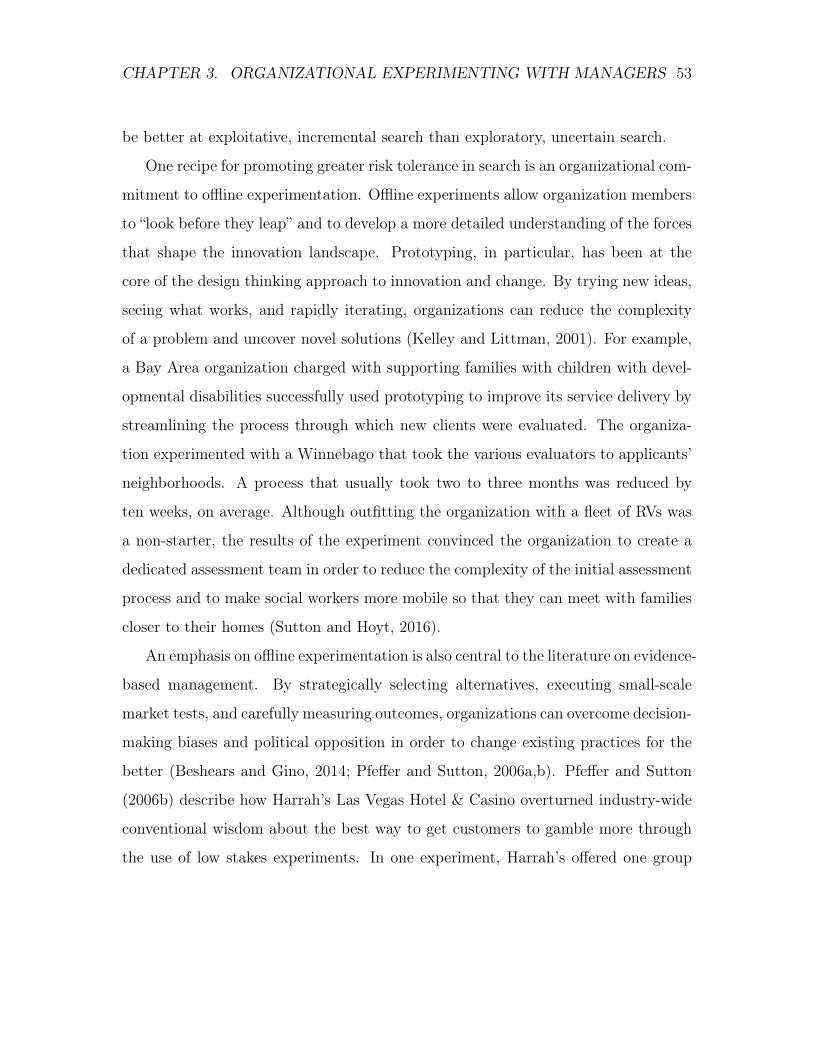
CHAPTER 3. ORGANIZATIONAL EXPERIMENTING WITH MANAGERS 53
be better at exploitative, incremental search than exploratory, uncertain search.
One recipe for promoting greater risk tolerance in search is an organizational com-
mitment to offline experimentation. Offline experiments allow organization members
to “look before they leap” and to develop a more detailed understanding of the forces
that shape the innovation landscape. Prototyping, in particular, has been at the
core of the design thinking approach to innovation and change. By trying new ideas,
seeing what works, and rapidly iterating, organizations can reduce the complexity
of a problem and uncover novel solutions (Kelley and Littman, 2001). For example,
a Bay Area organization charged with supporting families with children with devel-
opmental disabilities successfully used prototyping to improve its service delivery by
streamlining the process through which new clients were evaluated. The organiza-
tion experimented with a Winnebago that took the various evaluators to applicants’
neighborhoods. A process that usually took two to three months was reduced by
ten weeks, on average. Although outfitting the organization with a fleet of RVs was
a non-starter, the results of the experiment convinced the organization to create a
dedicated assessment team in order to reduce the complexity of the initial assessment
process and to make social workers more mobile so that they can meet with families
closer to their homes (Sutton and Hoyt, 2016).
An emphasis on offline experimentation is also central to the literature on evidence-
based management. By strategically selecting alternatives, executing small-scale
market tests, and carefully measuring outcomes, organizations can overcome decision-
making biases and political opposition in order to change existing practices for the
better (Beshears and Gino, 2014; Pfeffer and Sutton, 2006a,b). Pfeffer and Sutton
(2006b) describe how Harrah’s Las Vegas Hotel & Casino overturned industry-wide
conventional wisdom about the best way to get customers to gamble more through
the use of low stakes experiments. In one experiment, Harrah’s offered one group

CHAPTER 3. ORGANIZATIONAL EXPERIMENTING WITH MANAGERS 54
of customers a standard promotional package that included $30 in chips and $95
in meal and room vouchers and another group an experimental package that only
included $60 in chips. Contrary to the widely held belief that gamblers are enticed
to the tables by fancy meals and entertainment, the second package induced more
gambling revenue at a lower cost.
The economics literature on career concerns, however, paints a less rosy picture of
the capacity for organizations to motivate their employees to undertake exploratory
experiments, even if the outcomes of the experiments have low stakes for the organi-
zation. Managers who are unsure about their competence with a task would prefer
not to reveal information about their quality. Fear of being revealed as incapable
leads managers to forego risk taking, generating inertia, herding behavior, and pan-
dering (Aghion and Jackson, 2014; Canes-Wrone et al., 2001; Gibbons and Roberts,
2012). Canes-Wrone et al. (2001) describe how the re-election concerns of California
Governor and future Chief Justice of the United States Supreme Court Earl Warren
led him to pander to conservative fears about the threat of communism. Although
he initially objected indignantly to calls that UC-Berkeley faculty take an oath dis-
claiming membership in the Communist party, he later reversed course by making
such an oath a condition of all public employment. Warren was fearful that the
revelation of communist sympathies among state employees prior to his upcoming
election against staunch anti-Communist James Roosevelt could irreparably damage
his chances of winning. Requiring state employees to take an oath made him appear
strong against the communist threat.
A key insight of my paper is that career concerns can also lead managers to
be overly exploratory in their offline search behavior. Rather than implementing
an experimental strategy that a manager believes will work well, a manager may
instead experiment with a strategy that they know will likely go too far. Lindbergh
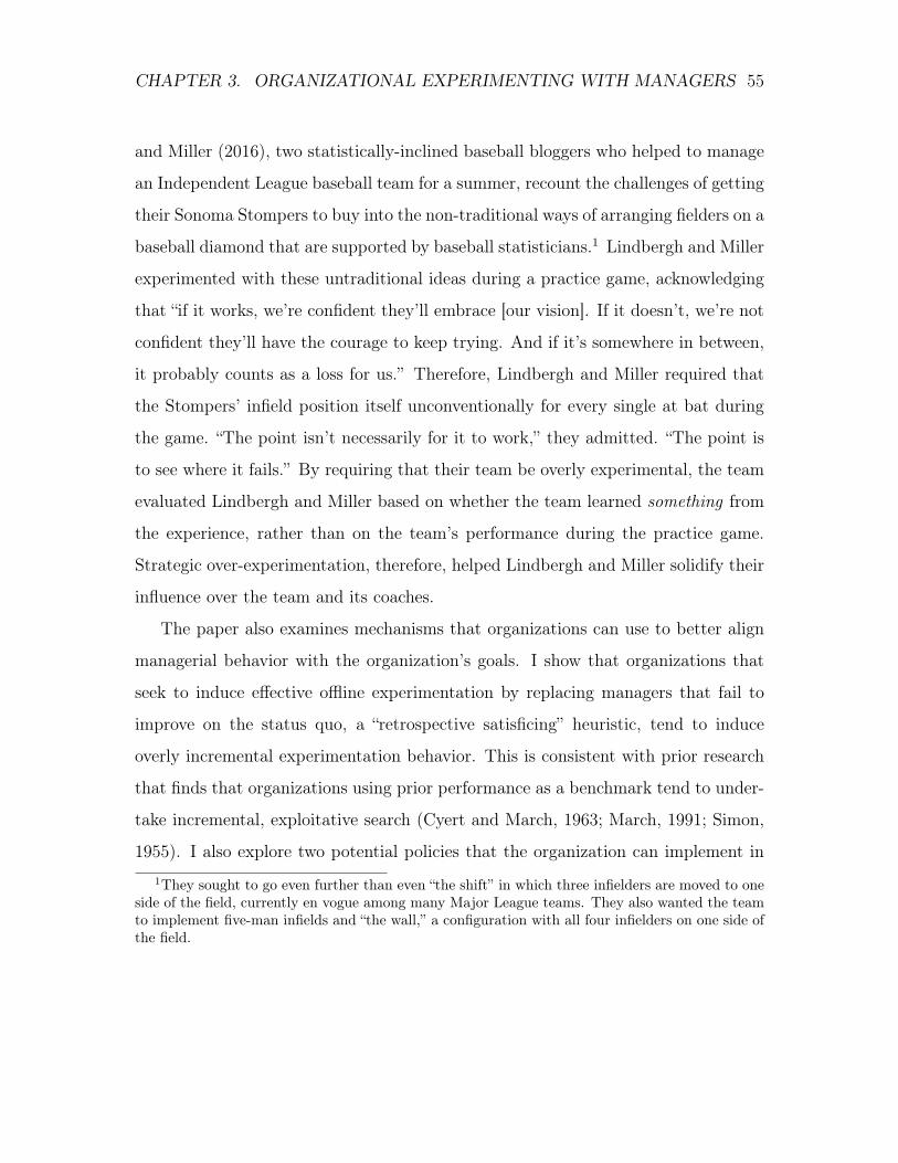
CHAPTER 3. ORGANIZATIONAL EXPERIMENTING WITH MANAGERS 55
and Miller (2016), two statistically-inclined baseball bloggers who helped to manage
an Independent League baseball team for a summer, recount the challenges of getting
their Sonoma Stompers to buy into the non-traditional ways of arranging fielders on a
baseball diamond that are supported by baseball statisticians.1 Lindbergh and Miller
experimented with these untraditional ideas during a practice game, acknowledging
that “if it works, we’re confident they’ll embrace [our vision]. If it doesn’t, we’re not
confident they’ll have the courage to keep trying. And if it’s somewhere in between,
it probably counts as a loss for us.” Therefore, Lindbergh and Miller required that
the Stompers’ infield position itself unconventionally for every single at bat during
the game. “The point isn’t necessarily for it to work,” they admitted. “The point is
to see where it fails.” By requiring that their team be overly experimental, the team
evaluated Lindbergh and Miller based on whether the team learned something from
the experience, rather than on the team’s performance during the practice game.
Strategic over-experimentation, therefore, helped Lindbergh and Miller solidify their
influence over the team and its coaches.
The paper also examines mechanisms that organizations can use to better align
managerial behavior with the organization’s goals. I show that organizations that
seek to induce effective offline experimentation by replacing managers that fail to
improve on the status quo, a “retrospective satisficing” heuristic, tend to induce
overly incremental experimentation behavior. This is consistent with prior research
that finds that organizations using prior performance as a benchmark tend to under-
take incremental, exploitative search (Cyert and March, 1963; March, 1991; Simon,
1955). I also explore two potential policies that the organization can implement in1They sought to go even further than even “the shift” in which three infielders are moved to one
side of the field, currently en vogue among many Major League teams. They also wanted the teamto implement five-man infields and “the wall,” a configuration with all four infielders on one side ofthe field.
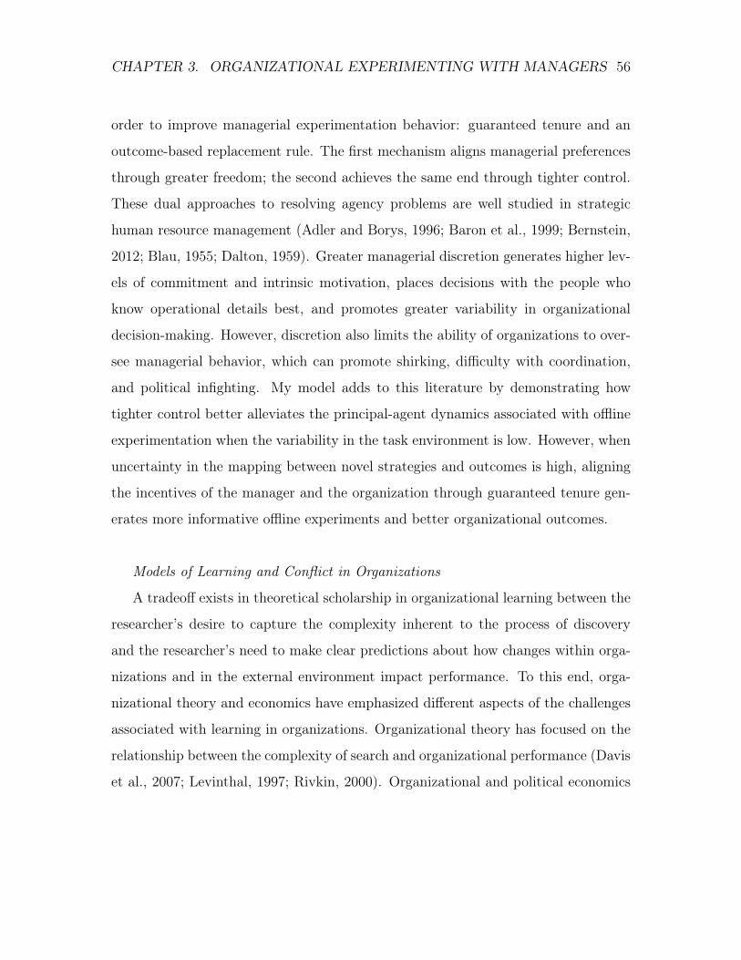
CHAPTER 3. ORGANIZATIONAL EXPERIMENTING WITH MANAGERS 56
order to improve managerial experimentation behavior: guaranteed tenure and an
outcome-based replacement rule. The first mechanism aligns managerial preferences
through greater freedom; the second achieves the same end through tighter control.
These dual approaches to resolving agency problems are well studied in strategic
human resource management (Adler and Borys, 1996; Baron et al., 1999; Bernstein,
2012; Blau, 1955; Dalton, 1959). Greater managerial discretion generates higher lev-
els of commitment and intrinsic motivation, places decisions with the people who
know operational details best, and promotes greater variability in organizational
decision-making. However, discretion also limits the ability of organizations to over-
see managerial behavior, which can promote shirking, difficulty with coordination,
and political infighting. My model adds to this literature by demonstrating how
tighter control better alleviates the principal-agent dynamics associated with offline
experimentation when the variability in the task environment is low. However, when
uncertainty in the mapping between novel strategies and outcomes is high, aligning
the incentives of the manager and the organization through guaranteed tenure gen-
erates more informative offline experiments and better organizational outcomes.
Models of Learning and Conflict in Organizations
A tradeoff exists in theoretical scholarship in organizational learning between the
researcher’s desire to capture the complexity inherent to the process of discovery
and the researcher’s need to make clear predictions about how changes within orga-
nizations and in the external environment impact performance. To this end, orga-
nizational theory and economics have emphasized different aspects of the challenges
associated with learning in organizations. Organizational theory has focused on the
relationship between the complexity of search and organizational performance (Davis
et al., 2007; Levinthal, 1997; Rivkin, 2000). Organizational and political economics

CHAPTER 3. ORGANIZATIONAL EXPERIMENTING WITH MANAGERS 57
has been concerned with problems associated with collecting and transmitting infor-
mation within organizations characterized by individuals with differing preferences
and goals (Callander, 2011a,b; Gibbons et al., 2012). My paper seeks to build on a
growing literature that spans these two views.
Within organizational theory, there is an emphasis on understanding how or-
ganizations react to randomness in the fitness landscape. These stochastic models
explore how uncertainty associated with the implementation of novel configurations
of organizational inputs combine with various search strategies to impact long-term
performance and rates of survival. The basic models in this tradition envision the
organization as undertaking random, local search and, through a process of trial-
and-error, eventually finding collections of inputs that dominate all other local com-
binations (Kauffman, 1993; Levinthal, 1997). However, more recent work has also
integrated cognitive representations of the fitness landscape that serve as maps for
evolutionary search. These cognitive maps take into account the roles of science and
abstract knowledge in the innovation process. Organizations cannot know precisely
how a change to a strategic input will impact performance, but organizations may
have general or abstract knowledge undergirding the innovation process that makes
it more likely that a particular change will be performance enhancing. (Csaszar and
Levinthal, 2016; Fleming and Sorenson, 2004; Gavetti and Levinthal, 2000). For
example, Fleming (2002) describes how the design of Hewlett-Packard’s first ink jet
printer was inspired by recent work in high temperature physics on “micro jets,” but
also required a lengthy trial-and-error experimental approach in order to find a resis-
tor that could both generate extreme heat and withstand long term wear-and-tear.
Other theoretical models of organizational search have also sought to integrate
more detailed descriptions of the decision-making process within organizations into
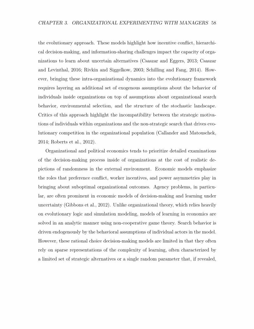
CHAPTER 3. ORGANIZATIONAL EXPERIMENTING WITH MANAGERS 58
the evolutionary approach. These models highlight how incentive conflict, hierarchi-
cal decision-making, and information-sharing challenges impact the capacity of orga-
nizations to learn about uncertain alternatives (Csaszar and Eggers, 2013; Csaszar
and Levinthal, 2016; Rivkin and Siggelkow, 2003; Schilling and Fang, 2014). How-
ever, bringing these intra-organizational dynamics into the evolutionary framework
requires layering an additional set of exogenous assumptions about the behavior of
individuals inside organizations on top of assumptions about organizational search
behavior, environmental selection, and the structure of the stochastic landscape.
Critics of this approach highlight the incompatibility between the strategic motiva-
tions of individuals within organizations and the non-strategic search that drives evo-
lutionary competition in the organizational population (Callander and Matouschek,
2014; Roberts et al., 2012).
Organizational and political economics tends to prioritize detailed examinations
of the decision-making process inside of organizations at the cost of realistic de-
pictions of randomness in the external environment. Economic models emphasize
the roles that preference conflict, worker incentives, and power asymmetries play in
bringing about suboptimal organizational outcomes. Agency problems, in particu-
lar, are often prominent in economic models of decision-making and learning under
uncertainty (Gibbons et al., 2012). Unlike organizational theory, which relies heavily
on evolutionary logic and simulation modeling, models of learning in economics are
solved in an analytic manner using non-cooperative game theory. Search behavior is
driven endogenously by the behavioral assumptions of individual actors in the model.
However, these rational choice decision-making models are limited in that they often
rely on sparse representations of the complexity of learning, often characterized by
a limited set of strategic alternatives or a single random parameter that, if revealed,
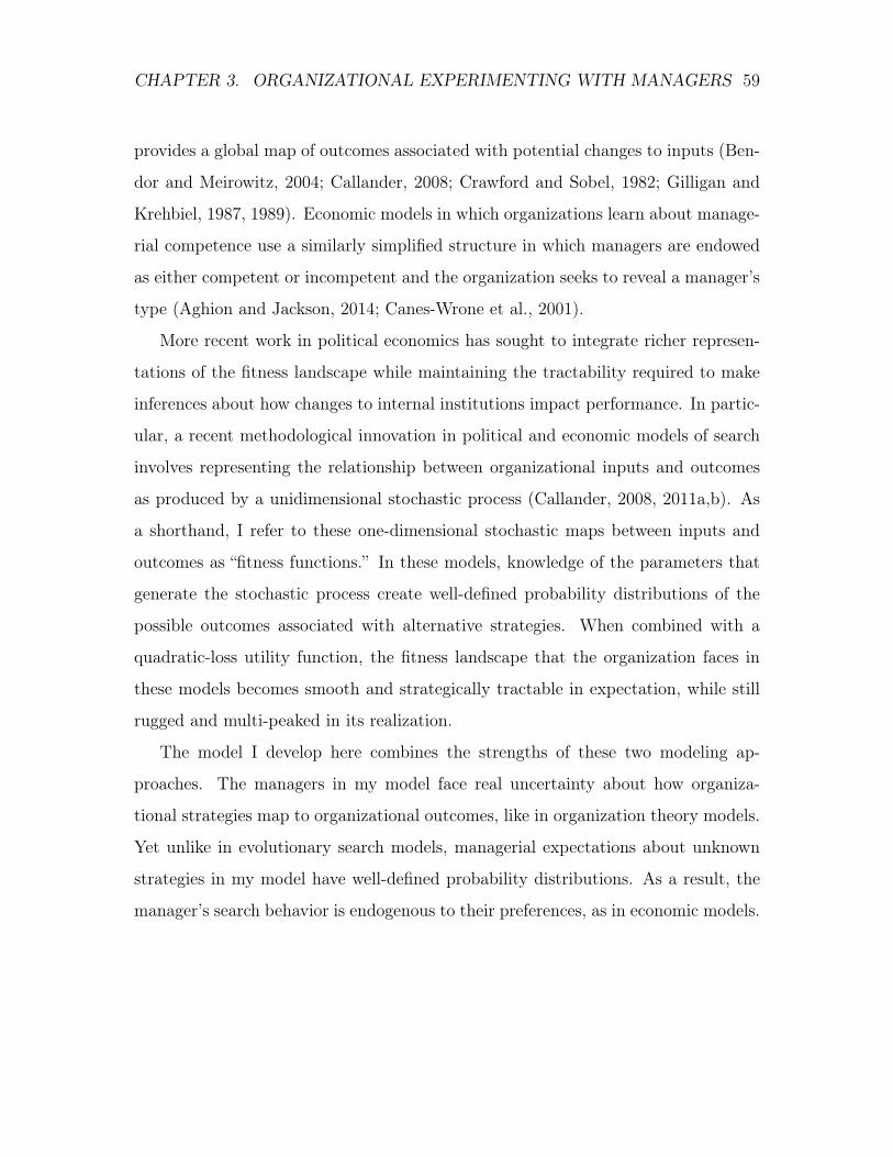
CHAPTER 3. ORGANIZATIONAL EXPERIMENTING WITH MANAGERS 59
provides a global map of outcomes associated with potential changes to inputs (Ben-
dor and Meirowitz, 2004; Callander, 2008; Crawford and Sobel, 1982; Gilligan and
Krehbiel, 1987, 1989). Economic models in which organizations learn about manage-
rial competence use a similarly simplified structure in which managers are endowed
as either competent or incompetent and the organization seeks to reveal a manager’s
type (Aghion and Jackson, 2014; Canes-Wrone et al., 2001).
More recent work in political economics has sought to integrate richer represen-
tations of the fitness landscape while maintaining the tractability required to make
inferences about how changes to internal institutions impact performance. In partic-
ular, a recent methodological innovation in political and economic models of search
involves representing the relationship between organizational inputs and outcomes
as produced by a unidimensional stochastic process (Callander, 2008, 2011a,b). As
a shorthand, I refer to these one-dimensional stochastic maps between inputs and
outcomes as “fitness functions.” In these models, knowledge of the parameters that
generate the stochastic process create well-defined probability distributions of the
possible outcomes associated with alternative strategies. When combined with a
quadratic-loss utility function, the fitness landscape that the organization faces in
these models becomes smooth and strategically tractable in expectation, while still
rugged and multi-peaked in its realization.
The model I develop here combines the strengths of these two modeling ap-
proaches. The managers in my model face real uncertainty about how organiza-
tional strategies map to organizational outcomes, like in organization theory models.
Yet unlike in evolutionary search models, managerial expectations about unknown
strategies in my model have well-defined probability distributions. As a result, the
manager’s search behavior is endogenous to their preferences, as in economic models.

CHAPTER 3. ORGANIZATIONAL EXPERIMENTING WITH MANAGERS 60
Further, the fitness function method I use here improves on prior work in organi-
zational economics by exploring the link between managerial incentives surrounding
tenure, managerial search behavior, and organizational performance. Rather than
a manager choosing between a risky and a safe option, which has been the norm
in economic models of career concerns, my model involves selecting amongst a con-
tinuum of interdependent experimental strategies. As a result, I make predictions
about how career concerns impact the character of experimentation that managers
undertake and how different experimentation strategies interact with the uncertainty
of the task environment to affect organizational performance.
The Model
The model features an organization that seeks to improve its performance by
delegating a new project to a tenure-motivated manager. The manager has the op-
portunity to prototype offline prior to the organization going online with the project.
After observing the prototype and the prototype’s performance, the organization’s
leadership has the opportunity to replace the manager. If the organization does not
replace the manager, then the same manager who experimented offline also takes the
project online. If the organization replaces the manager, a new manager is brought
in to take the project online.
Each manager in the organization is endowed with a unique fitness function, which
is represented by a realized path of Brownian motion. The parameters that generate
the stochastic Brownian path are publicly known and provide a baseline cognitive
representation for the relationship between untried strategies and outcomes. As a
manager experiments with new strategies and the associated outcomes are revealed,
the manager updates their cognitive map, in the process decreasing the variance in
the relationship between untried strategies and their outcomes. Importantly, when a
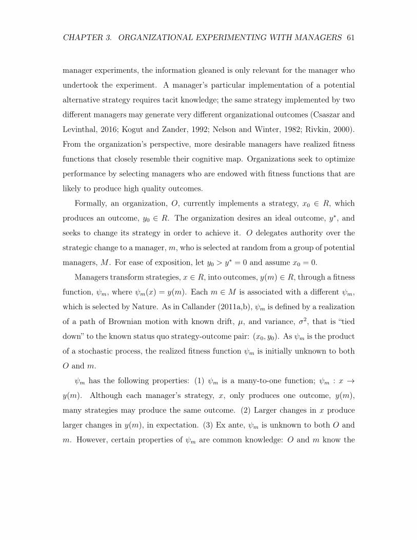
CHAPTER 3. ORGANIZATIONAL EXPERIMENTING WITH MANAGERS 61
manager experiments, the information gleaned is only relevant for the manager who
undertook the experiment. A manager’s particular implementation of a potential
alternative strategy requires tacit knowledge; the same strategy implemented by two
different managers may generate very different organizational outcomes (Csaszar and
Levinthal, 2016; Kogut and Zander, 1992; Nelson and Winter, 1982; Rivkin, 2000).
From the organization’s perspective, more desirable managers have realized fitness
functions that closely resemble their cognitive map. Organizations seek to optimize
performance by selecting managers who are endowed with fitness functions that are
likely to produce high quality outcomes.
Formally, an organization, O, currently implements a strategy, x0 2 R, which
produces an outcome, y0 2 R. The organization desires an ideal outcome, y⇤, and
seeks to change its strategy in order to achieve it. O delegates authority over the
strategic change to a manager, m, who is selected at random from a group of potential
managers, M . For ease of exposition, let y0 > y⇤ = 0 and assume x0 = 0.
Managers transform strategies, x 2 R, into outcomes, y(m) 2 R, through a fitness
function, m, where m(x) = y(m). Each m 2 M is associated with a different m,
which is selected by Nature. As in Callander (2011a,b), m is defined by a realization
of a path of Brownian motion with known drift, µ, and variance, �2, that is “tied
down” to the known status quo strategy-outcome pair: (x0, y0). As m is the product
of a stochastic process, the realized fitness function m is initially unknown to both
O and m.
m has the following properties: (1) m is a many-to-one function; m : x !
y(m). Although each manager’s strategy, x, only produces one outcome, y(m),
many strategies may produce the same outcome. (2) Larger changes in x produce
larger changes in y(m), in expectation. (3) Ex ante, m is unknown to both O and
m. However, certain properties of m are common knowledge: O and m know the

CHAPTER 3. ORGANIZATIONAL EXPERIMENTING WITH MANAGERS 62
expected change in y(m) given a one unit change in x, defined as µ. O and m also
know the variance of the distribution of possible outcomes associated with a one-unit
change in x, defined as �2. (4) With each observed pair of x and y(m), O and m
learn more about m and, as a result, predict how m maps from x to y(m) with
greater certainty.
µ and �2 are constant and m(x0) = y0 for all m 2 M . All that varies between
managers, therefore, is the stochastic realization of m. Ex ante, O is indifferent
between all m 2 M .
m has one opportunity to experiment offline with a prototype strategy, xp, prior
to the organization going online with an implemented strategy, x1. The experimen-
tation and implementation proceed as follows: In the first period, m selects xp. O
and m observe xp and yp(m). Then, O has the opportunity to replace m with m0,
who is another manager selected at random from M . m0 transforms strategies to
outcomes through the function m0 . In the second period, m or m0 implements x1
and, subsequently, y1(m) (or y1(m0)) is revealed.2 Importantly, m0 cannot use the
realization of (xp, yp(m)) to inform its choice of strategy. m0 has the same knowledge
of its own fitness function as m had prior to first period.
The utility for O is quadratic-loss: UO = �(y1 � y⇤)2 = �y21. Outcomes closer to
O’s ideal outcome, y⇤, are more desirable than those farther away. The quadratic-loss
utility function also makes O risk-averse such that EUO = �E(y1)2 � var(y1).
m and m0 have lexicographic preferences. Foremost, m is tenure-motivated. Um =
u if m is replaced and u if m is not replaced, where u < u. Secondarily, m and m0
have preferences that align with O’s. (As m0 only has one period of tenure, m0 has
preferences, therefore, that fully align with O’s and will select x1 to maximize EUO.)2From this point forward, both y1(m) and y1(m0) will be referred to as y1 unless it is necessary
to be explicit about whether m or m0 is in charge of implementation in the second period.
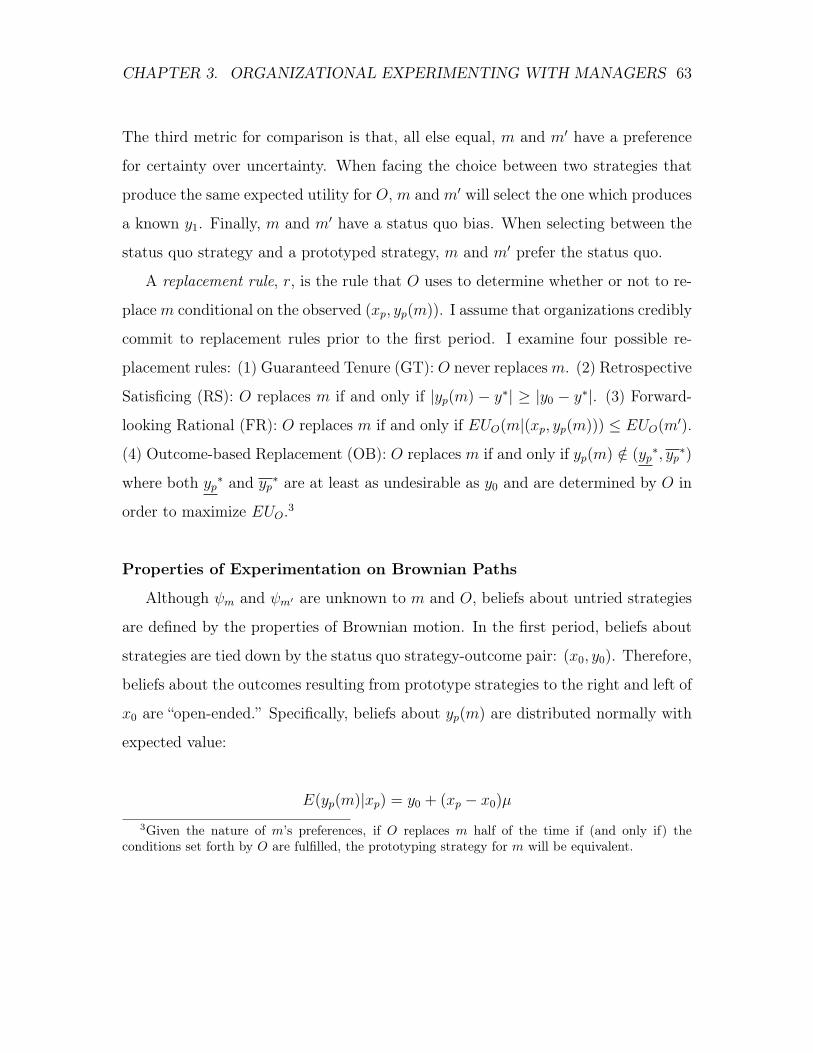
CHAPTER 3. ORGANIZATIONAL EXPERIMENTING WITH MANAGERS 63
The third metric for comparison is that, all else equal, m and m0 have a preference
for certainty over uncertainty. When facing the choice between two strategies that
produce the same expected utility for O, m and m0 will select the one which produces
a known y1. Finally, m and m0 have a status quo bias. When selecting between the
status quo strategy and a prototyped strategy, m and m0 prefer the status quo.
A replacement rule, r, is the rule that O uses to determine whether or not to re-
place m conditional on the observed (xp, yp(m)). I assume that organizations credibly
commit to replacement rules prior to the first period. I examine four possible re-
placement rules: (1) Guaranteed Tenure (GT): O never replaces m. (2) Retrospective
Satisficing (RS): O replaces m if and only if |yp(m) � y⇤| � |y0 � y⇤|. (3) Forward-
looking Rational (FR): O replaces m if and only if EUO(m|(xp, yp(m))) EUO(m0).
(4) Outcome-based Replacement (OB): O replaces m if and only if yp(m) /2 (yp⇤, yp
⇤)
where both yp⇤ and yp
⇤ are at least as undesirable as y0 and are determined by O in
order to maximize EUO.3
Properties of Experimentation on Brownian Paths
Although m and m0 are unknown to m and O, beliefs about untried strategies
are defined by the properties of Brownian motion. In the first period, beliefs about
strategies are tied down by the status quo strategy-outcome pair: (x0, y0). Therefore,
beliefs about the outcomes resulting from prototype strategies to the right and left of
x0 are “open-ended.” Specifically, beliefs about yp(m) are distributed normally with
expected value:
E(yp(m)|xp) = y0 + (xp � x0)µ
3Given the nature of m’s preferences, if O replaces m half of the time if (and only if) theconditions set forth by O are fulfilled, the prototyping strategy for m will be equivalent.
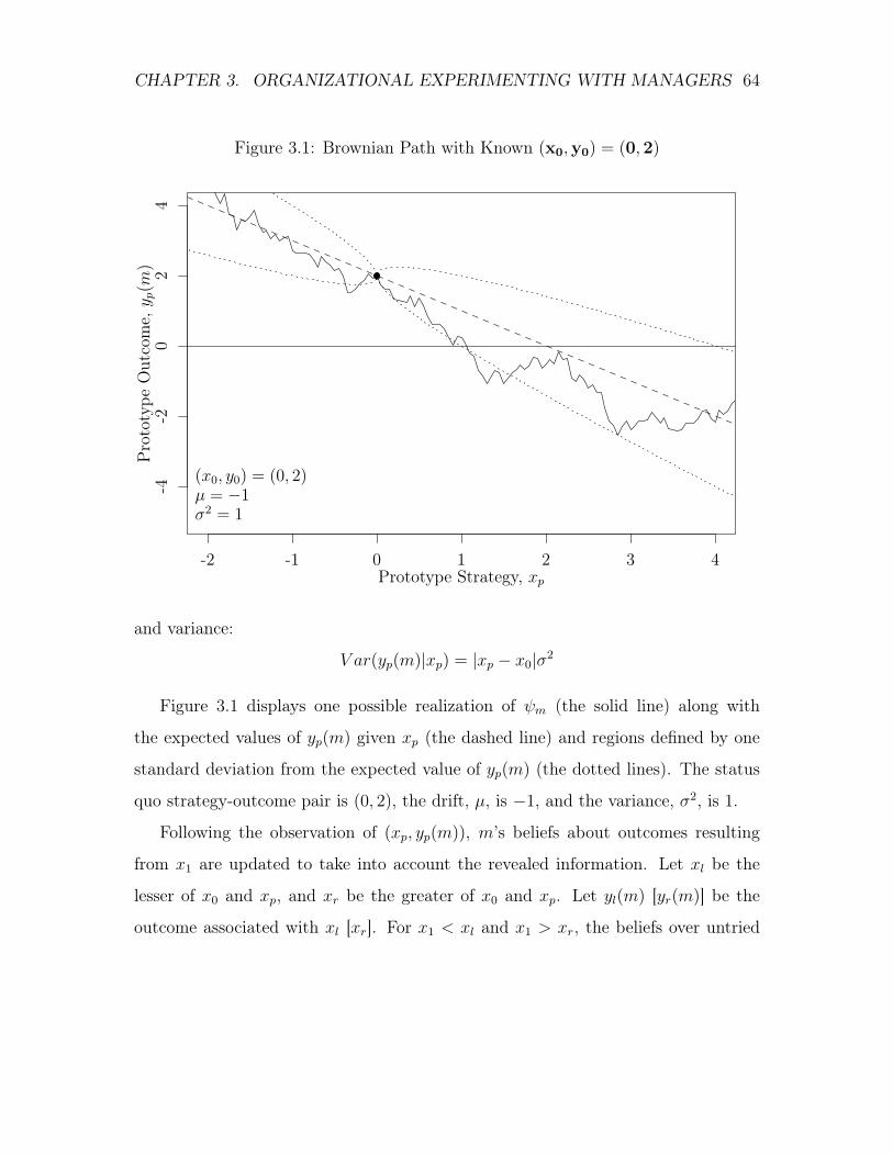
CHAPTER 3. ORGANIZATIONAL EXPERIMENTING WITH MANAGERS 64
Figure 3.1: Brownian Path with Known (x0,y0) = (0,2)
-2 -1 0 1 2 3 4
-4-2
02
4
Prototype Strategy, xp
Pro
toty
peO
utco
me,
y p(m)
(x0, y0) = (0, 2)µ = �1
�2= 1
and variance:
V ar(yp(m)|xp) = |xp � x0|�2
Figure 3.1 displays one possible realization of m (the solid line) along with
the expected values of yp(m) given xp (the dashed line) and regions defined by one
standard deviation from the expected value of yp(m) (the dotted lines). The status
quo strategy-outcome pair is (0, 2), the drift, µ, is �1, and the variance, �2, is 1.
Following the observation of (xp, yp(m)), m’s beliefs about outcomes resulting
from x1 are updated to take into account the revealed information. Let xl be the
lesser of x0 and xp, and xr be the greater of x0 and xp. Let yl(m) [yr(m)] be the
outcome associated with xl [xr]. For x1 < xl and x1 > xr, the beliefs over untried
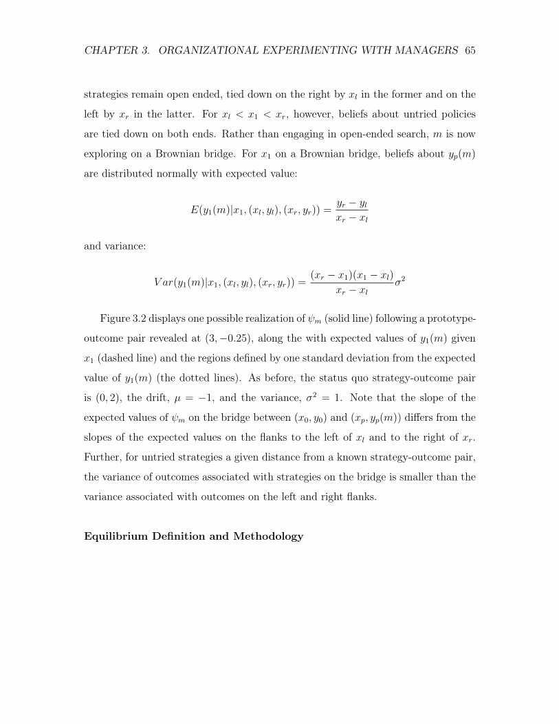
CHAPTER 3. ORGANIZATIONAL EXPERIMENTING WITH MANAGERS 65
strategies remain open ended, tied down on the right by xl in the former and on the
left by xr in the latter. For xl < x1 < xr, however, beliefs about untried policies
are tied down on both ends. Rather than engaging in open-ended search, m is now
exploring on a Brownian bridge. For x1 on a Brownian bridge, beliefs about yp(m)
are distributed normally with expected value:
E(y1(m)|x1, (xl, yl), (xr, yr)) =yr � ylxr � xl
and variance:
V ar(y1(m)|x1, (xl, yl), (xr, yr)) =(xr � x1)(x1 � xl)
xr � xl
�2
Figure 3.2 displays one possible realization of m (solid line) following a prototype-
outcome pair revealed at (3,�0.25), along the with expected values of y1(m) given
x1 (dashed line) and the regions defined by one standard deviation from the expected
value of y1(m) (the dotted lines). As before, the status quo strategy-outcome pair
is (0, 2), the drift, µ = �1, and the variance, �2= 1. Note that the slope of the
expected values of m on the bridge between (x0, y0) and (xp, yp(m)) differs from the
slopes of the expected values on the flanks to the left of xl and to the right of xr.
Further, for untried strategies a given distance from a known strategy-outcome pair,
the variance of outcomes associated with strategies on the bridge is smaller than the
variance associated with outcomes on the left and right flanks.
Equilibrium Definition and Methodology
CHAPTER 3. ORGANIZATIONAL EXPERIMENTING WITH MANAGERS 66
Figure 3.2: Brownian Path with Known (x0,y0) = (0,2) and(xp,yp(m)) = (3,�0.25)
-1 0 1 2 3 4
-10
12
34
Implemented Strategy, x1
Fina
lOut
com
e,y 1(m)
(x0, y0) = (0, 2)(xp, yp(m)) = (3,�0.25)µ = �1
�2= 1

CHAPTER 3. ORGANIZATIONAL EXPERIMENTING WITH MANAGERS 67
I utilize a subgame perfect equilibrium concept. As the game proceeds sequen-
tially and there is perfect information, there exists a unique subgame perfect equi-
librium.
I solve the game through backwards induction. The second period equilibrium
strategies for m and m0, x⇤1(m) and x⇤
1(m0), are defined as in Callander (2011a,
2011b). The first period equilibrium strategy for m, defined as x⇤p(r), is the xp that
maximizes EUm conditional on replacement rule r, where r 2 {GT,RS, FR,OR}.
The equilibrium replacement rules for O define conditions under which O will
replace m. For O 2 {GT,RS}, the replacement rules for O are self-explanatory.
For r = FR, the prototype-outcome pairs for which O replaces m, indicated by
(xp,yp)⇤FR, are defined such that if (xp, yp) 2 (xp,yp)
⇤FR, then EUO(m|x⇤
1(m), (xp, yp))
EUO(m0|x⇤
1(m0)). For r = OB, the boundaries assigned in equilibrium by O, (yp⇤, yp⇤),
are defined in order to maximize EUO subject to the best response by m, x⇤p(OB).
In order to find x⇤p, I rely on a combination of analytical methods and compu-
tation. I find the analytic solution for x⇤1(m) conditional on µ, �2, (x0, y0), and
(xp, yp(m)). I also find the analytic solution for x⇤1(m
0) conditional on µ, �2, and
(x0, y0). The nature of the replacement regimes and the properties of Brownian
motion preclude explicit analytic solutions for x⇤p(r). As a result, I define implicit
solutions for x⇤p conditional on µ, �2, r, x⇤
1(m), and x⇤1(m
0). I then solve for x⇤
p(r)
using numerical optimization methods.
I demonstrate x⇤p and EUO(x
⇤p) for a range of y0 > 0 and �2 under different
replacement rules. For analytic simplicity, I fix µ = �1. y0 represents the extent
to which O is dissatisfied with the status quo. �2 represents the complexity of the
problem that the managers face.4
4Callander (2011a; 2011b) demonstrates that search behavior in models of this sort is determinedby the ratio of the increase in uncertainty given a one unit change in x and the change in y given
CHAPTER 3. ORGANIZATIONAL EXPERIMENTING WITH MANAGERS 68
Analytical Results
In order to solve the model by backwards induction, I first find x⇤1(m) and x⇤
1(m0)
given (x0, y0), (xp, yp(m)), µ, and �. For m and m0, preferences are aligned with O
in the second period. As a result, m and m0 face a problem (nearly) identical to the
one analyzed in Callander (2011a; 2011b). Therefore, Propositions 1 and 2a-2g and
Lemmas 1a-1d are direct applications of Callander (2011a; 2011b).
Second Period Behavior
I first examine x⇤1(m
0). As m has been replaced and the information revealed
during prototyping is of no value to m0, m0 selects x1 based on their beliefs about
m0 in order to maximize EUm0 . This is equivalent to maximizing EUO = �(y1�y⇤)2.
There are three possible strategic changes available to m0 in the second period. m0
can choose not to make a revision to x0, which I describe as a stable strategy. m0 can
choose to make a revision to x0 such that x1 > x0, which I describe as a rightward
change. m0 can also choose the make a revision to x0 such that x1 < x0, a left-
ward change. However, given that y0 > 0 and µ < 0, a leftward change, which moves
y1(m0) further away from y⇤ in expectation, is strictly dominated by a stable strategy.
Lemma 1a: For y0 > �2
2 , the optimal x1 for m0, x⇤1(m
0), produces an expected
outcome of �2
2 . For y0 �2
2 , x⇤1(m) is stable at x0.
Risk aversion leads m0 to aim for an outcome that is between the status quo
outcome and their ideal outcome of 0. The boundary at which the utility sacrificed
from the additional variance associated with more exploration exceeds the utility
benefit from a more desirable outcome in expectation is half the complexity of the
a one unit change in x. Therefore, generality is maintained by assuming µ = �1.

CHAPTER 3. ORGANIZATIONAL EXPERIMENTING WITH MANAGERS 69
search environment, �2
2 . For status quo outcomes outside of the boundary, m0 will
search rightward. For status quo outcomes interior to the boundary, m0 will prefer
the status quo outcome to the risk associated with rightward search.
Proposition 1: The optimal x1 for m0, x⇤1(m) is:
• If y0 > �2
2 , x⇤1(m
0) = y0 � �2
2 . EUO = �(y0 � �2
4 )�2.
• If y0 �2
2 , x⇤1(m
0) = x0. EUO = �y20.
For y0 that is sufficiently distant from y⇤, m0 explores to the right of x0 in order
to seek a more desirable outcome. For y0 sufficiently close to y⇤, m0 prefers a stable
strategy in which it retains the status quo, x0, than to explore and bear the associ-
ated risk of a bad outcome.
Next, I examine the optimal x1 for m, x⇤1(m), conditional on the realization of
(xp, yp(m)). The strategy depends crucially on whether yp(m) has moved backwards
and away from y0, moved towards y0 but still short of y⇤, or moved past y⇤.
There are five possible strategic changes available to m in the second period,
conditional on (xp, yp(m)). m can retain xp, which I describe as a stable strategy. m
can choose to return to x0, which I describe as backsliding. m can choose x1 > xr,
where xr = max(x0, xp), a rightward change. m can xl < x1 < xr, which I de-
scribe as a change on the Brownian bridge. Finally, m can choose x1 < xl, where
xl = min(x0, xp), a leftward change.
First, I explore the dominant second period strategy for m if m chooses to retain
the status quo and forego the opportunity to prototype. In such a case, the strategic
CHAPTER 3. ORGANIZATIONAL EXPERIMENTING WITH MANAGERS 70
decision for m in the second period is equivalent to the strategic decision for m0 in
the second period.
Proposition 2a: If xp = x0, then x⇤1(m) = x⇤
1(m0).
Now, I move on to the (more interesting) cases where xp 6= x0. I first ex-
amine the conditions under which backsliding is the dominant strategy for m for
yp(m) > y⇤ = 0.
Lemma 1b: For yp(m) > 0, a leftward change is strictly dominated by a stable
strategy if yp(m) y0; or a backsliding strategy if yp(m) > y0.
As a leftward strategy moves y1 away from y⇤ for yp(m) > 0, m prefers to retain
the known strategy-outcome pair that is closest to y⇤ than to revise its strategy left-
ward.
Lemma 1c: For yp(m) > �2
2 and xp > 0, rightward exploration dominates retaining
the prototype strategy.
After observing yp(m), m chooses whether to continue to search rightward, to
keep the prototype strategy, or to backslide to x0. Lemma 1b notes that, when
choosing between the first two options, m prefers to retain the prototype xp if xp
is sufficiently close to y⇤. Otherwise, m prefers to explore rightward than to retain xp.
Proposition 2b: For values of �2 and y0 and realizations of (xp, yp(m)) that satisfy
the following conditions, the optimal x1 for m, x⇤1(m), involves backsliding to x0.
• If y0 > �2
2 and yp(m) � y20+�2/4
�2 and xp > x0, x⇤1(m) = x0. EUO = �y20.

CHAPTER 3. ORGANIZATIONAL EXPERIMENTING WITH MANAGERS 71
• If y0 �2
2 and yp(m) � y0, x⇤1(m) = x0. EUO = �y20.
For observed yp(m) sufficiently far away from y⇤ and xp > x0, m prefers to back-
slide to x0 rather than to continue to explore to the right from xp and take on the
associated uncertainty. For all yp(m) > y0 and for y0 sufficiently close to y⇤ (i.e.
y0 �2
2 ), m prefers to backslide to x0 than to either retain xp or search rightward.
For y0 sufficiently far from the ideal outcome (i.e. y0 > �2
2 ) and yp(m) > y0, m
weighs the expected utility associated with exploring rightward with the expected
utility from backsliding to x0. For yp(m) > y0 and yp(m) >> y⇤, m backslides.
For yp(m) closer to y⇤ but not so close as to be desirable in and of itself, a back-
sliding strategy is dominated by a rightward change.
Proposition 2c: For values of �2 and y0 and realizations of (xp, yp(m)) that satisfy
the following conditions, x⇤1(m) involves a rightward revision.
• If y0 > �2
2 and yp(m) <y20+�
2/4�2 < �2
2 and xp > x0, x⇤1(m) = yp(m) � �2
2 .
EUO = �(yp(m)� �2
4 )�2.
• If y0 > �2
2 and yp(m) >q
(y0 � �2
4 )�2 and xp < x0, x⇤
1(m) = y0 � �2
2 . EUO =
�(y0 � �2
4 )�2.
For yp(m) far enough away from y⇤ as to make continued search desirable (but
not so far as to make rightward search less desirable than backsliding) and xp > x0,
m continues to search to the right from xp. For xp < x0, unless xp is sufficiently close
to y⇤ as to make it desirable to be retained, m searches to the right from x0 in period 2.
For yp(m) sufficiently close to y⇤, m retains yp(m) rather than risk the uncer-
tainty associated with revising its strategy. I first consider offline prototypes for
CHAPTER 3. ORGANIZATIONAL EXPERIMENTING WITH MANAGERS 72
which yp(m) is still short of y⇤ and m chooses to retain yp(m).
Proposition 2d: For values of �2 and y0 and realizations of (xp, yp(m)) that satisfy
the following conditions, x⇤1(m) is stable at xp.
• If �2
2 � yp(m) � 0 and xp > x0, x⇤1(m) = xp. EUO = �yp(m)
2.
• Ifq
(y0 � �2
4 )�2 � xp � 0 and xp < x0, x⇤
1(m) = xp. EUO = �yp(m)
2.
If the prototype outcome is sufficiently close to y⇤ and involved a rightward re-
vision from x0, then m retains xp. In contrast, if the prototype involved a leftward
revision, then m compares the known utility from remaining at xp to the expected
utility from a rightward change from x0.
I now move on to yp(m) < y0 and xp > 0.5 For yp(m) < y0, m has the opportunity
to experiment on the Brownian bridge and reap the gains associated with the de-
creased variance. However, for strategy-outcome pairs for which yp(m) is sufficiently
close to y⇤, m still prefers a stable strategy.
Lemma 1d: For yp(m) < 0 and xp < x0, a rightward change is dominated by xp.
Because the prototype has overshot its target, further exploration to the right
only brings m further from the organization’s goal, in expectation.
Proposition 2e: For values of �2 and y0 and realizations of (xp, yp(m)) that satisfy
the following conditions, x⇤1(m) is stable at xp.
5Note that I do not characterize x⇤1 for yp(m) < 0 and xp < x0. Solving for x⇤
1 in these cases isnot necessary to characterize x⇤
p(r) for any of the replacement rules as first-period outcomes in thisregion are fairly unlikely. Further, the optimal behavior of m in these cases is (perhaps surprisingly)complex to define explicitly.
CHAPTER 3. ORGANIZATIONAL EXPERIMENTING WITH MANAGERS 73
• If 0 > yp(m) � �y0 and yp(m) � � �2
2|µ| where µ =
yp
(m)�y0xp
, x⇤1(m) = xp.
EUO = �yp(m)
2.
Note that the boundary of yp(m) for which m prefers the known xp to exper-
imenting on the bridge grows more extreme as the expected slope of m on the
bridge becomes shallower. Bigger experiments require larger differences in outcomes
in order to warrant further experimentation in the second period.
However, for sufficiently large first period experiments (i.e., xp >> 0), yp can be
further from y⇤ than y0, yet experimenting on the bridge is still undesirable. As a re-
sult, rather than remaining stable at xp, m backslides to x0, as EUm(x0) > EUm(xp).
Proposition 2f: For values of �2 and y0 and realizations of (xp, yp(m)) that satisfy
the following conditions, x⇤1(m) backslides to x0.
• If yp(m) �y0 and y0 �2
2|µ| , x⇤1(m) = x0, EUO = �y20.
For more extreme values of yp(m), the expected slope is sufficiently large to in-
duce experimentation on the bridge. x⇤1(m) lies between x0 and xp. If y0 is more
desirable than yp, x⇤1(m) < x
p
2 and E(y1) > 0. Otherwise, x⇤1(m) > x
p
2 and E(y1) < 0.
Proposition 2g: For values of �2 and y0 and realizations of (xp, yp(m)) that satisfy
the following conditions, x⇤1(m) is on the bridge spanning (x0, y0) and (xp, yp(m)).
• If yp(m) < � �2
2|µ| , or yp(m) > y0 and y0 >�2
2|µ| :
x⇤1(m) =
2µy0 + �2
2
⇣�2
xp
� µ2⌘
EUO = �(y0 + µx⇤1(m))
2 � (xp � x⇤1(m))x⇤
1(m)
xp
�2
CHAPTER 3. ORGANIZATIONAL EXPERIMENTING WITH MANAGERS 74
I graphically depict x⇤1(m) given (xp, yp(m)) and �2
= 1. In Figure 3.3, y0 is
sufficiently undesirable as to induce rightward search for some yp > 0. In contrast,
in Figure 3.4, y0 is fairly close to y⇤, which makes rightward search undesirable for
yp > 0.
Replacement Rules and Prototyping Strategies
I now examine the prototyping behavior of m and replacement decisions of O in
greater detail.
Under Guaranteed Tenure, r = GT , the replacement rule fully aligns the pref-
erences of m and O. As a result, m selects x⇤p(GT ) in order to maximize EUO in
period 2 under the assumption that m will not be replaced. Guaranteed Tenure
produces the same behavior for m in equilibrium as if O implemented a replacement
rule in which O assigns m a prototype strategy x⇤⇤p and replaces m if and only if
xp(m) 6= x⇤⇤p .
Note, however, that if there were no principal-agent problems (i.e. m were not
tenure motivated) and m were replaced after period 1 if EUO/m(m) < EUO/m(m0),
x⇤p(GT ) would not be the utility-maximizing level of xp. If m were revealed to be
a poor fit for the task, m would prefer to be replaced with m0 rather than being
retained. This inefficiency associated with being forced to retain an undesirable m
under Guaranteed Tenure leads to an conservative bias in x⇤p(GT ) relative to the
optimal experiment under fully aligned preferences. However, x⇤p(GT ) is equivalent
to the utility-maximizing xp for O when m0 is incapable of improving on the status
quo, which is the case when y0 < �2
2 , or when the fitness functions of potential re-
placements are identical to m’s, i.e. m(x) = m0(x) for all m0 2 M and for all x 2 R.
Proposition 3: x⇤p(GT ) is defined implicitly by the following equation:
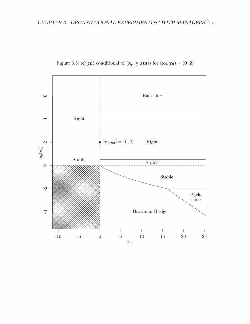
CHAPTER 3. ORGANIZATIONAL EXPERIMENTING WITH MANAGERS 75
Figure 3.3: x
⇤1(m) conditional of (xp,yp(m)) for (x0,y0) = (0,2)
-10 -5 0 5 10 15 20 25
-4-2
02
46
xp
y p(m)
Right
Backslide
Right
StableStable
Stable
Brownian Bridge
Back-slide
(x0, y0) = (0, 2)
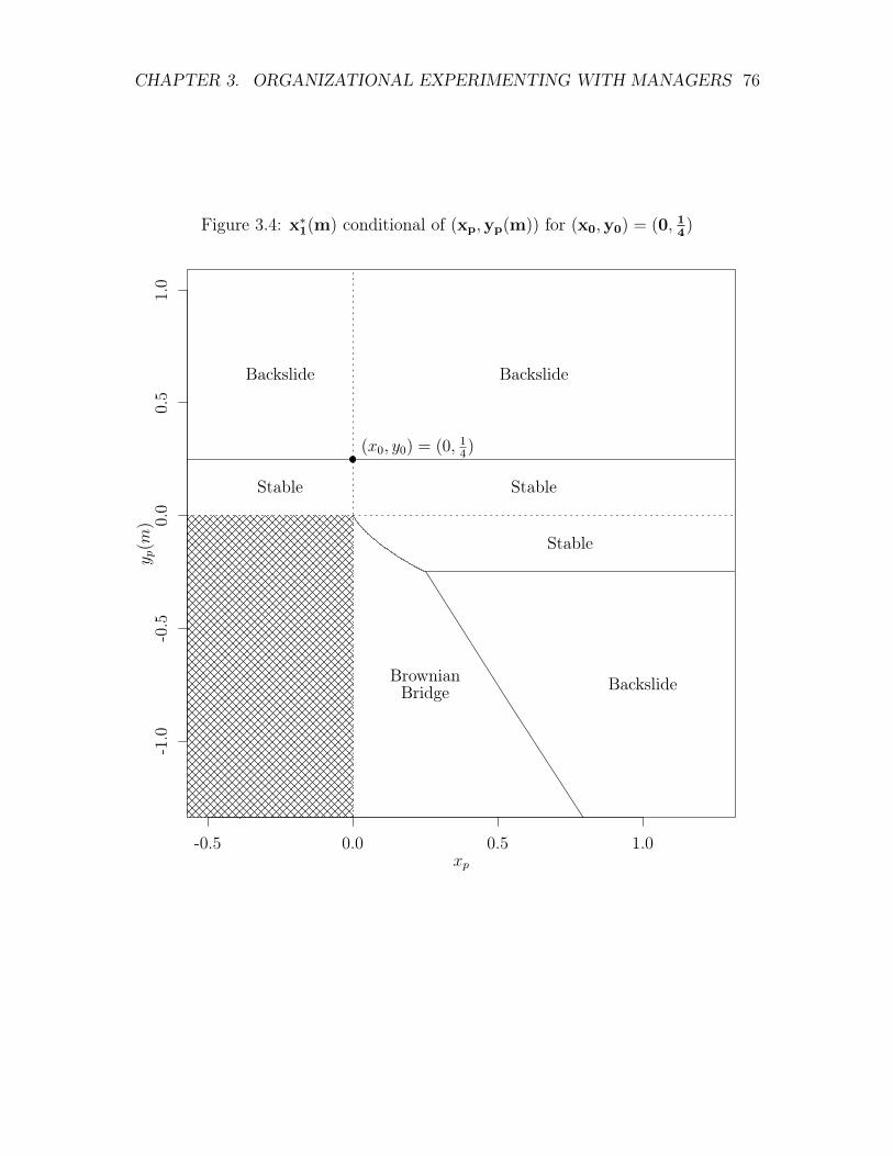
CHAPTER 3. ORGANIZATIONAL EXPERIMENTING WITH MANAGERS 76
Figure 3.4: x
⇤1(m) conditional of (xp,yp(m)) for (x0,y0) = (0, 14)
-0.5 0.0 0.5 1.0
-1.0
-0.5
0.0
0.5
1.0
xp
y p(m)
Backslide Backslide
Stable Stable
Stable
BackslideBrownianBridge
(x0, y0) = (0, 14)
CHAPTER 3. ORGANIZATIONAL EXPERIMENTING WITH MANAGERS 77
max
xp
EUO(y1|x⇤1(m), x1(m
0) = x0)
Under the Retrospective Satisficing replacement rule, r = RS, O will replace
m if yp is not closer to y⇤ than y0. x⇤p(RS) is, therefore, the prototyping strategy
that maximizes the probability that y0 > |yp|. It is important that m be replaced if
|yp| = y0 in order to induce m to experiment at all.
Proposition 4: x⇤p(RS) is unique and defined implicitly by the following equation:
max
xp
"�
xpp�2xp
!� �
xp � 2y0p
�2xp
!#
One property of x⇤p(RS) is that it exhibits risk aversion. As larger experiments
generate more uncertainty, m will choose a prototype strategy which produces an
outcome that falls short of y⇤, in expectation.
Lemma 2a: x⇤p(RS) > 0 and E( m(x
⇤p(RS))) < y⇤.
Uniqueness and risk aversion, in fact, reflects a more general property of replace-
ment rules in which yp must fall between y0 and a lower bound, yp, in order for m to
be retained. Under a replacement rule of this sort, EUm(xp) is quasi-concave in xp
for xp > 0. Furthermore, E( m(x⇤p(RS))) always falls short of the midpoint between
the upper and lower boundary.
Lemma 2b: For any replacement regime in which m is replaced if yp /2 (yp, y0),
CHAPTER 3. ORGANIZATIONAL EXPERIMENTING WITH MANAGERS 78
x⇤p(RS) is unique and in (0,
y0�yp
2 ).
Under the Forward-Looking Rational replacement rule, r = FR, O will replace m
when EUO(m|x⇤1(m), (xp, yp(m))) EUO(m
0|x⇤1(m
0)). There are two regions where
this will be the case. First, if yp(m) > y0, then m is less attractive than m0 because
m has to search farther to the right than m0 to reach y⇤. Second, in the regions
where xp > 0 and yp(m) < 0 in which m backslides to x0, m0 can do at least as well
as m by keeping x0 (or improve on x0 by experimenting to the right for y0 >�2
2 ).
In equilibrium, m, therefore, searches to the right until there exist values of yp(m)
given xp that will lead O to replace m. This strategy minimizes the probability that
yp(m) > y0 without adding an additional risk of replacement.
Proposition 5: If y0 > �2
2 , then x⇤p(FR) � 4y0��2. If y0 �2
2 , then x⇤p(FR) =
4y20�2 .
Lemma 3: If the first derivative of the values of (xp, yp) that satisfy EUO(m, (xp, yp)) =
EUO(m0) is less than �1 for y0 >
�2
2 , then x⇤p(FR) = 4y0 � �2.
An Outcome-based replacement rule is similar to Retrospective Satisficing, in
that if yp fails to fall between an upper and lower bound, m will be replaced by m0.
However, Outcome-based replacement allows O to set the upper and lower bound to
be more extreme than y0 and �y0 in order to induce a more desirable first period
experiment than x⇤p(RS). However, the rule has the downside of requiring that O
replace m when yp yp, even when the expected utility of retaining m exceeds the
expected utility of replacing m.
Under Outcome-based replacement, the upper bound, yp⇤ is equal to y0 in equilib-
rium. If it were greater than y0, then m would select xp = x0 and never be replaced.
CHAPTER 3. ORGANIZATIONAL EXPERIMENTING WITH MANAGERS 79
Therefore, O adjusts yp⇤ in order to induce the desired x⇤
p(OB).
Proposition 6a: yp⇤= y0. yp
⇤ is defined implicitly by the following equation:
max
yp
EUO(x⇤p(OB), x⇤
1(m), x⇤1(m
0))
m selects xp in a similar fashion to the Retrospective Satisficing replacement rule,
although with a lower bound of yp rather than �y0.
Proposition 6b: x⇤p(OB) is defined implicitly by the following equation, where yp
indicates the lower bound for acceptable outcomes defined by O. For a given yp,
there is a unique induced x⇤p(OB) that maximizes the equation.
max
xp
"�
xpp�2xp
!� �
xp + yp � y0p�2xp
!#
Whereas Guaranteed Tenure sometimes forces O to keep m when it would prefer
to replace m, Outcome-based replacement requires that O sometimes replace m when
O would prefer to keep m. Therefore, when choosing between these two replacement
regimes, O trades off the cost of keeping an undesirable m with replacing a desirable
one.
Proposition 7: O weakly prefers r = GT to r = OB when EUO(x⇤p(GT )) �
EUO(x⇤p(OB)). O weakly prefers r = OB to r = GT when EUO(x
⇤p(GT ))
EUO(x⇤p(OB)). O strictly prefers r = GT to r = OB if y0 �2
2 .
CHAPTER 3. ORGANIZATIONAL EXPERIMENTING WITH MANAGERS 80
Computational Approach
I briefly describe how I computationally derive equilibrium outcomes for x⇤p(r).
All global optimizations use either golden-section search, simulated annealing or
genetic optimization, implemented using the stats, GenSA and rgenoud packages
in R-3.2.1. Appendix B offers an annotated version of the scripts used to calculate
all of the examples in the paper.
I use golden-section optimization or simulated annealing when I can demonstrate
analytically that the function EUm(xp) is quasi-concave in the relevant region. I
use simulated annealing when the bounds on x⇤p(r) are analytically defined but the
function to be optimized is not shown to be quasi-concave, as simulated annealing
tends to be very efficient for unidimensional global optimization subject to a box
constraint (Mullen, 2014). I use genetic optimization when the bounds are not ana-
lytically defined, as genetic optimization allows for the algorithm to explore beyond
predetermined bounds. For more detail on the simulated annealing algorithm, see
Xiang et al. (2013). For more detail on the genetic optimization algorithm, see
Mebane Jr. and Sekhon (2011).
Computational Results
I evaluate the first-period experimentation strategy subject to the various re-
placement rules.
Figure 3.5 demonstrates EUm and EUO conditional on xp under Guaranteed
Tenure for �2 2 {1, 2, 4} and y0 2 {12 , 1, 2, 4} for xp 2 [0, 2y0]. The gray lines indicate
x⇤p. As the preferences of m are aligned with O, the expected utilities of m and O
are equal. Further, EUm appears quasi-concave with respect to xp for the values
depicted. Finally, the utility curves are proportional when the ratios of the distance
from the status quo outcome to the optimal outcome (i.e. y0) and the complexity
CHAPTER 3. ORGANIZATIONAL EXPERIMENTING WITH MANAGERS 81
of the fitness function (i.e. �2) are equal. (See, for example, �2= 1, y0 = 1 vs.
�2= 2, y0 = 2 vs. �2
= 4, y0 = 4.) This property will hold for all of the replacement
rules.
Figure 3.6 graphs x⇤p conditional on y0 as a function of �2. Most striking is the
non-monotonic relationship between optimal experimentation behavior and the com-
plexity of the task environment. For tasks of low to moderate complexity, optimal
experimentation involves shooting past the ideal outcome (i.e. E( m(xp)) < 0) and
then triangulating on a Brownian bridge in the second period. This makes intuitive
sense. In low complexity task environments, the modest increased uncertainty asso-
ciated with the bigger first period experiment is outstripped by the gains associated
with lower uncertainty in the implementation phase. However, for more complex
environments, the uncertainty associated with a big first period experiment swamps
the benefits from possibly triangulating on a Brownian bridge in the second period.
Further, the optimal experiment is always strictly positive, but approaches zero
as complexity increases. It is always beneficial for m to undertake some experi-
mentation in the first period, because m can backslide in the second period if the
experimental outcome is undesirable. However, for environments characterized by
explosive uncertainty, m makes a very incremental experiment in the hope of moving
marginally closer to the ideal outcome than the status quo. Note that, in expectation,
this sort of experimentation behavior will lead to outcomes that are incrementally
more desirable than the status quo. Approximately half of the time the organization
ends up backsliding to the status quo after observing the experimental outcome.
Finally, as in Figure 3.5, the shapes of the x⇤p functions are proportional. When
the range of �2 is scaled by y0, the four functions are identical in shape, although
varied in the magnitude of x⇤p. This property will also hold for all of the replacement
rules.
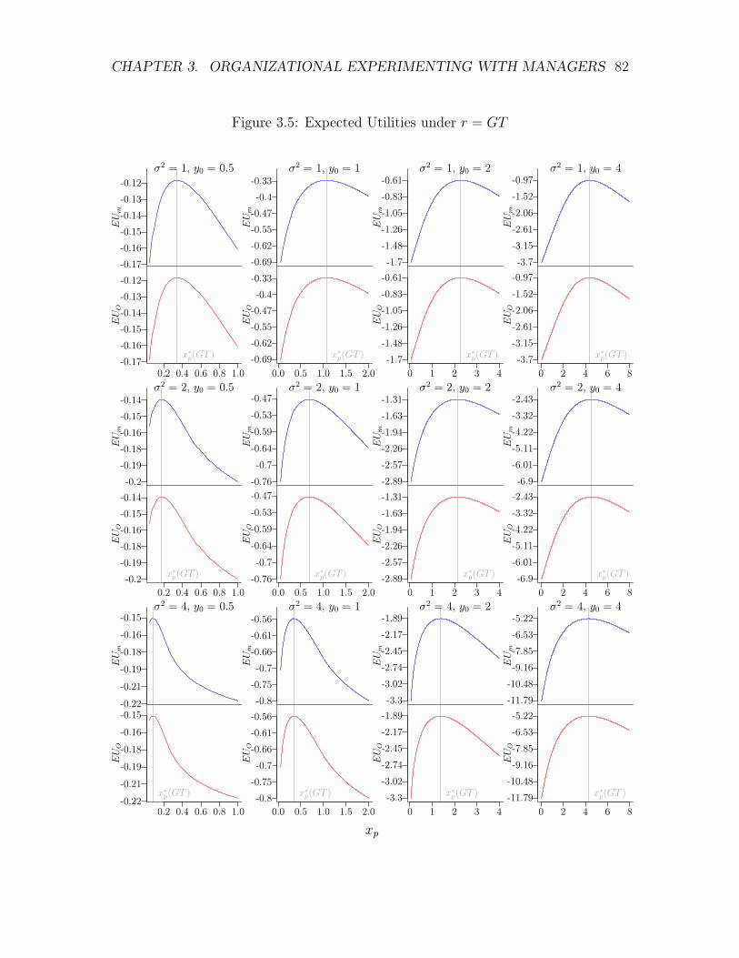
CHAPTER 3. ORGANIZATIONAL EXPERIMENTING WITH MANAGERS 82
Figure 3.5: Expected Utilities under r = GT
x
EUm
-0.17-0.16-0.15-0.14-0.13-0.12
�2= 1, y0 = 0.5
x
EUO
-0.17-0.16-0.15-0.14-0.13-0.12
0.2 0.4 0.6 0.8 1.0
x⇤p(GT )
x
EUm
-0.69-0.62-0.55-0.47-0.4
-0.33�2
= 1, y0 = 1
x
EUO
-0.69-0.62-0.55-0.47-0.4
-0.33
0.0 0.5 1.0 1.5 2.0
x⇤p(GT )
x
EUm
-1.7-1.48-1.26-1.05-0.83-0.61
�2= 1, y0 = 2
xEUO
-1.7-1.48-1.26-1.05-0.83-0.61
0 1 2 3 4
x⇤p(GT )
x
EUm
-3.7-3.15-2.61-2.06-1.52-0.97
�2= 1, y0 = 4
x
EUO
-3.7-3.15-2.61-2.06-1.52-0.97
0 2 4 6 8
x⇤p(GT )
x
EUm
-0.2-0.19-0.18-0.16-0.15-0.14
�2= 2, y0 = 0.5
x
EUO
-0.2-0.19-0.18-0.16-0.15-0.14
0.2 0.4 0.6 0.8 1.0
x⇤p(GT )
x
EUm
-0.76-0.7
-0.64-0.59-0.53-0.47
�2= 2, y0 = 1
x
EUO
-0.76-0.7
-0.64-0.59-0.53-0.47
0.0 0.5 1.0 1.5 2.0
x⇤p(GT )
x
EUm
-2.89-2.57-2.26-1.94-1.63-1.31
�2= 2, y0 = 2
x
EUO
-2.89-2.57-2.26-1.94-1.63-1.31
0 1 2 3 4
x⇤p(GT )
xEUm
-6.9-6.01-5.11-4.22-3.32-2.43
�2= 2, y0 = 4
x
EUO
-6.9-6.01-5.11-4.22-3.32-2.43
0 2 4 6 8
x⇤p(GT )
x
EUm
-0.22
-0.21
-0.19
-0.18
-0.16
-0.15�2
= 4, y0 = 0.5
x
EUO
-0.22
-0.21
-0.19
-0.18
-0.16
-0.15
0.2 0.4 0.6 0.8 1.0
x⇤p(GT )
x
EUm
-0.8-0.75-0.7
-0.66-0.61-0.56
�2= 4, y0 = 1
x
EUO
-0.8-0.75-0.7
-0.66-0.61-0.56
0.0 0.5 1.0 1.5 2.0
x⇤p(GT )
x
EUm
-3.3-3.02-2.74-2.45-2.17-1.89
�2= 4, y0 = 2
x
EUO
-3.3-3.02-2.74-2.45-2.17-1.89
0 1 2 3 4
x⇤p(GT )
x
EUm
-11.79-10.48-9.16-7.85-6.53-5.22
�2= 4, y0 = 4
x
EUO
-11.79-10.48-9.16-7.85-6.53-5.22
0 2 4 6 8
x⇤p(GT )
xp
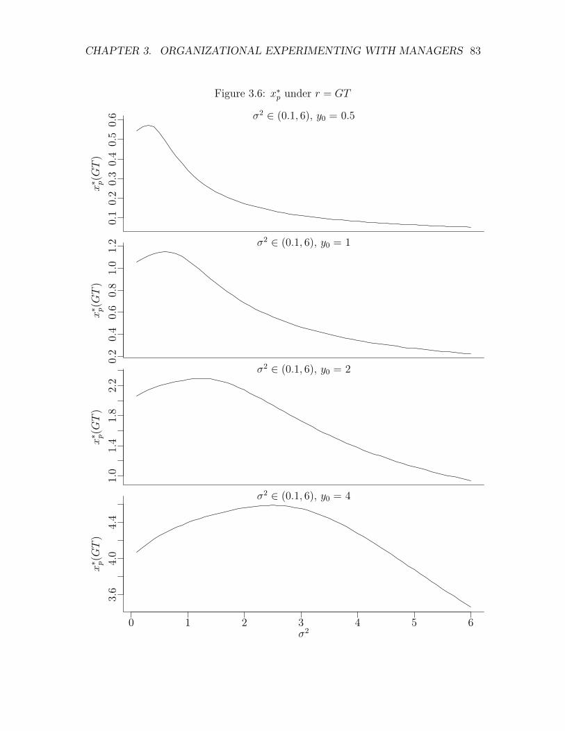
CHAPTER 3. ORGANIZATIONAL EXPERIMENTING WITH MANAGERS 83
Figure 3.6: x⇤p under r = GT
s2
x⇤ p(GT)
0.1
0.2
0.3
0.4
0.5
0.6 �2 2 (0.1, 6), y0 = 0.5
s2
x⇤ p(GT)
0.2
0.4
0.6
0.8
1.0
1.2 �2 2 (0.1, 6), y0 = 1
s2
x⇤ p(GT)
1.0
1.4
1.8
2.2
�2 2 (0.1, 6), y0 = 2
s2
x⇤ p(GT)
3.6
4.0
4.4
�2 2 (0.1, 6), y0 = 4
0 1 2 3 4 5 6�2
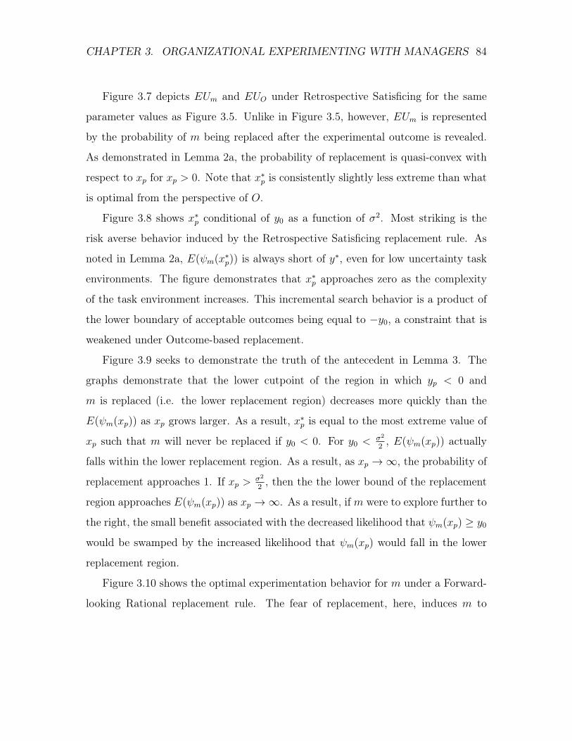
CHAPTER 3. ORGANIZATIONAL EXPERIMENTING WITH MANAGERS 84
Figure 3.7 depicts EUm and EUO under Retrospective Satisficing for the same
parameter values as Figure 3.5. Unlike in Figure 3.5, however, EUm is represented
by the probability of m being replaced after the experimental outcome is revealed.
As demonstrated in Lemma 2a, the probability of replacement is quasi-convex with
respect to xp for xp > 0. Note that x⇤p is consistently slightly less extreme than what
is optimal from the perspective of O.
Figure 3.8 shows x⇤p conditional of y0 as a function of �2. Most striking is the
risk averse behavior induced by the Retrospective Satisficing replacement rule. As
noted in Lemma 2a, E( m(x⇤p)) is always short of y⇤, even for low uncertainty task
environments. The figure demonstrates that x⇤p approaches zero as the complexity
of the task environment increases. This incremental search behavior is a product of
the lower boundary of acceptable outcomes being equal to �y0, a constraint that is
weakened under Outcome-based replacement.
Figure 3.9 seeks to demonstrate the truth of the antecedent in Lemma 3. The
graphs demonstrate that the lower cutpoint of the region in which yp < 0 and
m is replaced (i.e. the lower replacement region) decreases more quickly than the
E( m(xp)) as xp grows larger. As a result, x⇤p is equal to the most extreme value of
xp such that m will never be replaced if y0 < 0. For y0 < �2
2 , E( m(xp)) actually
falls within the lower replacement region. As a result, as xp ! 1, the probability of
replacement approaches 1. If xp >�2
2 , then the the lower bound of the replacement
region approaches E( m(xp)) as xp ! 1. As a result, if m were to explore further to
the right, the small benefit associated with the decreased likelihood that m(xp) � y0
would be swamped by the increased likelihood that m(xp) would fall in the lower
replacement region.
Figure 3.10 shows the optimal experimentation behavior for m under a Forward-
looking Rational replacement rule. The fear of replacement, here, induces m to
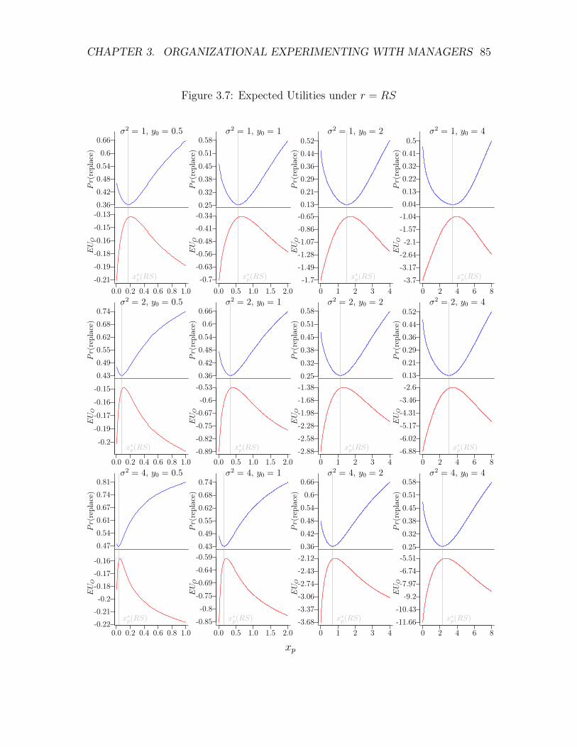
CHAPTER 3. ORGANIZATIONAL EXPERIMENTING WITH MANAGERS 85
Figure 3.7: Expected Utilities under r = RS
x
Pr(
repl
ace)
0.360.420.480.540.6
0.66�2
= 1, y0 = 0.5
x
EUO
-0.21-0.19-0.18
-0.16-0.15-0.13
0.0 0.2 0.4 0.6 0.8 1.0
x⇤p(RS)
x
Pr(
repl
ace)
0.250.320.380.450.510.58
�2= 1, y0 = 1
x
EUO
-0.7-0.63-0.56-0.48-0.41-0.34
0.0 0.5 1.0 1.5 2.0
x⇤p(RS)
x
Pr(
repl
ace)
0.130.210.290.360.440.52
�2= 1, y0 = 2
xEUO
-1.7-1.49-1.28-1.07-0.86-0.65
0 1 2 3 4
x⇤p(RS)
x
Pr(
repl
ace)
0.040.130.220.320.410.5
�2= 1, y0 = 4
x
EUO
-3.7-3.17-2.64-2.1
-1.57-1.04
0 2 4 6 8
x⇤p(RS)
x
Pr(
repl
ace)
0.430.490.550.620.680.74
�2= 2, y0 = 0.5
x
EUO
-0.2
-0.19
-0.17
-0.16
-0.15
0.0 0.2 0.4 0.6 0.8 1.0
x⇤p(RS)
x
Pr(
repl
ace)
0.360.420.480.540.6
0.66�2
= 2, y0 = 1
x
EUO
-0.89-0.82-0.75-0.67-0.6
-0.53
0.0 0.5 1.0 1.5 2.0
x⇤p(RS)
x
Pr(
repl
ace)
0.250.320.380.450.510.58
�2= 2, y0 = 2
x
EUO
-2.88-2.58-2.28-1.98-1.68-1.38
0 1 2 3 4
x⇤p(RS)
xPr(
repl
ace)
0.130.210.290.360.440.52
�2= 2, y0 = 4
x
EUO
-6.88-6.02-5.17-4.31-3.46-2.6
0 2 4 6 8
x⇤p(RS)
x
Pr(
repl
ace)
0.470.540.610.670.740.81
�2= 4, y0 = 0.5
x
EUO
-0.22-0.21-0.2
-0.18-0.17-0.16
0.0 0.2 0.4 0.6 0.8 1.0
x⇤p(RS)
x
Pr(
repl
ace)
0.430.490.550.620.680.74
�2= 4, y0 = 1
x
EUO
-0.85-0.8
-0.75-0.69-0.64-0.59
0.0 0.5 1.0 1.5 2.0
x⇤p(RS)
x
Pr(
repl
ace)
0.360.420.480.540.6
0.66�2
= 4, y0 = 2
x
EUO
-3.68-3.37-3.06-2.74-2.43-2.12
0 1 2 3 4
x⇤p(RS)
x
Pr(
repl
ace)
0.250.320.380.450.510.58
�2= 4, y0 = 4
x
EUO
-11.66-10.43
-9.2-7.97-6.74-5.51
0 2 4 6 8
x⇤p(RS)
xp
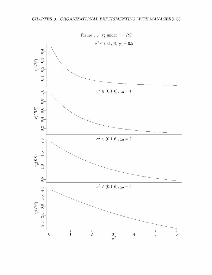
CHAPTER 3. ORGANIZATIONAL EXPERIMENTING WITH MANAGERS 86
Figure 3.8: x⇤p under r = RS
s2
x⇤ p(RS)
0.1
0.2
0.3
0.4
�2 2 (0.1, 6), y0 = 0.5
s2
x⇤ p(RS)
0.2
0.4
0.6
0.8
1.0 �2 2 (0.1, 6), y0 = 1
s2
x⇤ p(RS)
0.5
1.0
1.5
2.0 �2 2 (0.1, 6), y0 = 2
s2
x⇤ p(RS)
2.0
2.5
3.0
3.5
4.0 �2 2 (0.1, 6), y0 = 4
0 1 2 3 4 5 6�2
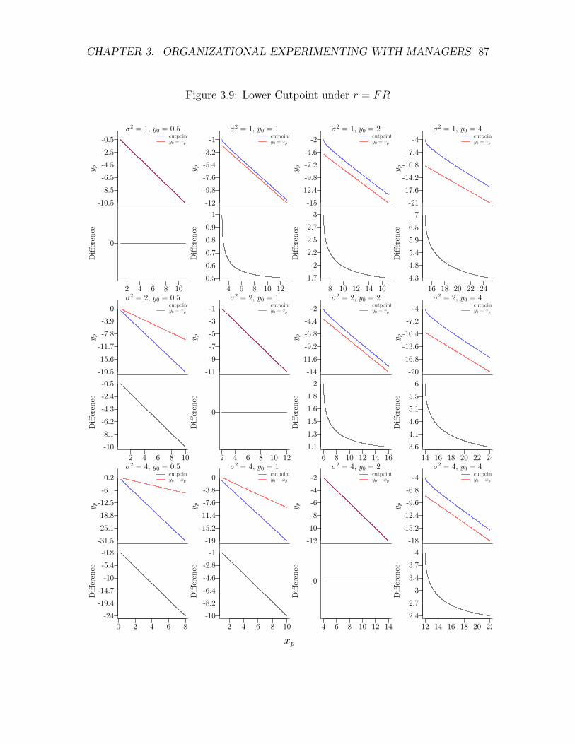
CHAPTER 3. ORGANIZATIONAL EXPERIMENTING WITH MANAGERS 87
Figure 3.9: Lower Cutpoint under r = FR
x
y p
-10.5-8.5-6.5-4.5-2.5-0.5 cutpoint
y0 � xp
�2= 1, y0 = 0.5
Diff
eren
ce
0
2 4 6 8 10
x
y p-12-9.8-7.6-5.4-3.2
-1 cutpointy0 � xp
�2= 1, y0 = 1
Diff
eren
ce
0.50.60.70.80.9
1
4 6 8 10 12
x
y p
-15-12.4-9.8-7.2-4.6
-2 cutpointy0 � xp
�2= 1, y0 = 2
Diff
eren
ce
1.72
2.22.52.7
3
8 10 12 14 16
x
y p
-21-17.6-14.2-10.8-7.4
-4 cutpointy0 � xp
�2= 1, y0 = 4
Diff
eren
ce
4.34.85.45.96.5
7
16 18 20 22 24
x
y p
-19.5-15.6-11.7-7.8-3.9
0 cutpointy0 � xp
�2= 2, y0 = 0.5
Diff
eren
ce
-10-8.1-6.2-4.3-2.4-0.5
2 4 6 8 10
x
y p
-11-9-7-5-3-1 cutpoint
y0 � xp
�2= 2, y0 = 1
Diff
eren
ce
0
2 4 6 8 10 12
x
y p
-14-11.6-9.2-6.8-4.4
-2 cutpointy0 � xp
�2= 2, y0 = 2
Diff
eren
ce
1.11.31.51.61.8
2
6 8 10 12 14 16
xy p
-20-16.8-13.6-10.4-7.2
-4 cutpointy0 � xp
�2= 2, y0 = 4
Diff
eren
ce
3.64.14.65.15.5
6
14 16 18 20 22 24
x
y p
-31.5-25.1-18.8-12.5-6.10.2 cutpoint
y0 � xp
�2= 4, y0 = 0.5
Diff
eren
ce
-24-19.4-14.7
-10-5.4-0.8
0 2 4 6 8
x
y p
-19-15.2-11.4-7.6-3.8
0 cutpointy0 � xp
�2= 4, y0 = 1
Diff
eren
ce
-10-8.2-6.4-4.6-2.8
-1
2 4 6 8 10
x
y p
-12-10-8-6-4-2 cutpoint
y0 � xp
�2= 4, y0 = 2
Diff
eren
ce
0
4 6 8 10 12 14
x
y p
-18-15.2-12.4-9.6-6.8
-4 cutpointy0 � xp
�2= 4, y0 = 4
Diff
eren
ce
2.42.7
33.43.7
4
12 14 16 18 20 22
xp
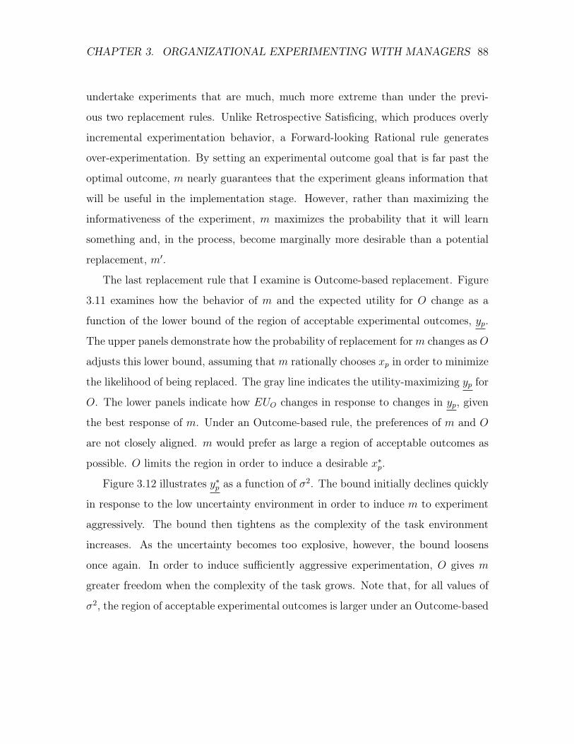
CHAPTER 3. ORGANIZATIONAL EXPERIMENTING WITH MANAGERS 88
undertake experiments that are much, much more extreme than under the previ-
ous two replacement rules. Unlike Retrospective Satisficing, which produces overly
incremental experimentation behavior, a Forward-looking Rational rule generates
over-experimentation. By setting an experimental outcome goal that is far past the
optimal outcome, m nearly guarantees that the experiment gleans information that
will be useful in the implementation stage. However, rather than maximizing the
informativeness of the experiment, m maximizes the probability that it will learn
something and, in the process, become marginally more desirable than a potential
replacement, m0.
The last replacement rule that I examine is Outcome-based replacement. Figure
3.11 examines how the behavior of m and the expected utility for O change as a
function of the lower bound of the region of acceptable experimental outcomes, yp.
The upper panels demonstrate how the probability of replacement for m changes as O
adjusts this lower bound, assuming that m rationally chooses xp in order to minimize
the likelihood of being replaced. The gray line indicates the utility-maximizing yp for
O. The lower panels indicate how EUO changes in response to changes in yp, given
the best response of m. Under an Outcome-based rule, the preferences of m and O
are not closely aligned. m would prefer as large a region of acceptable outcomes as
possible. O limits the region in order to induce a desirable x⇤p.
Figure 3.12 illustrates y⇤p as a function of �2. The bound initially declines quickly
in response to the low uncertainty environment in order to induce m to experiment
aggressively. The bound then tightens as the complexity of the task environment
increases. As the uncertainty becomes too explosive, however, the bound loosens
once again. In order to induce sufficiently aggressive experimentation, O gives m
greater freedom when the complexity of the task grows. Note that, for all values of
�2, the region of acceptable experimental outcomes is larger under an Outcome-based
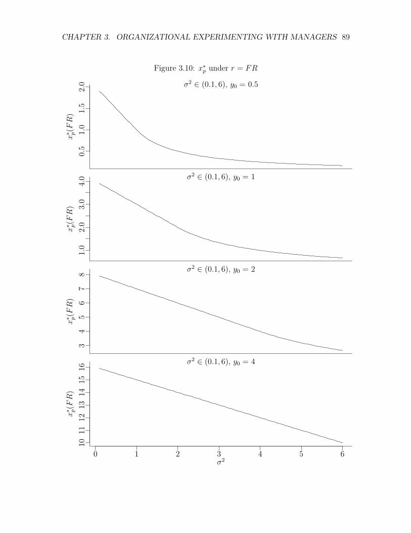
CHAPTER 3. ORGANIZATIONAL EXPERIMENTING WITH MANAGERS 89
Figure 3.10: x⇤p under r = FR
s2
x⇤ p(FR)
0.5
1.0
1.5
2.0 �2 2 (0.1, 6), y0 = 0.5
s2
x⇤ p(FR)
1.0
2.0
3.0
4.0 �2 2 (0.1, 6), y0 = 1
s2
x⇤ p(FR)
34
56
78 �2 2 (0.1, 6), y0 = 2
s2
x⇤ p(FR)
1011
1213
1415
16
�2 2 (0.1, 6), y0 = 4
0 1 2 3 4 5 6�2
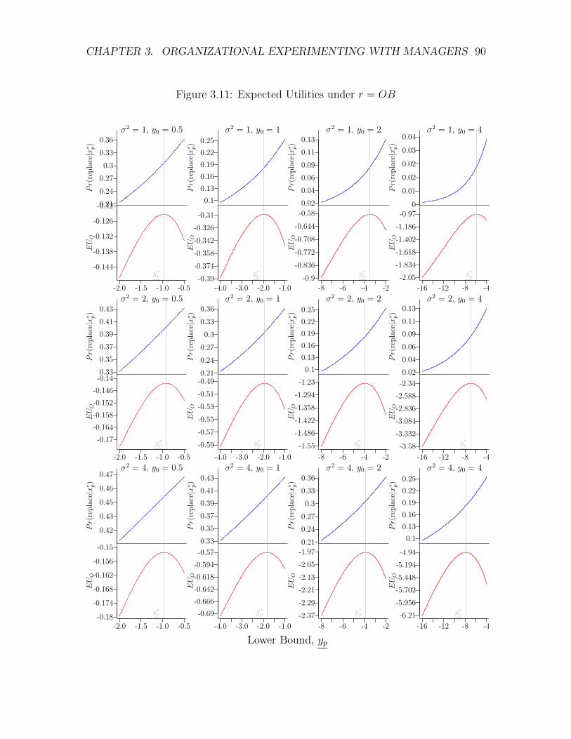
CHAPTER 3. ORGANIZATIONAL EXPERIMENTING WITH MANAGERS 90
Figure 3.11: Expected Utilities under r = OB
x
Pr(
repl
ace|x⇤ p)
0.210.240.270.3
0.330.36
�2= 1, y0 = 0.5
x
EUO
-0.144
-0.138
-0.132
-0.126
-0.12
-2.0 -1.5 -1.0 -0.5
y⇤p
x
Pr(
repl
ace|x⇤ p)
0.10.130.160.190.220.25
�2= 1, y0 = 1
x
EUO
-0.39-0.374-0.358-0.342-0.326-0.31
-4.0 -3.0 -2.0 -1.0
y⇤p
x
Pr(
repl
ace|x⇤ p)
0.020.040.060.090.110.13
�2= 1, y0 = 2
x
EUO
-0.9
-0.836
-0.772
-0.708
-0.644
-0.58
-8 -6 -4 -2
y⇤p
x
Pr(
repl
ace|x⇤ p)
0
0.01
0.02
0.02
0.03
0.04�2
= 1, y0 = 4
x
EUO
-2.05-1.834-1.618-1.402-1.186-0.97
-16 -12 -8 -4
y⇤p
x
Pr(
repl
ace|x⇤ p)
0.330.350.370.390.410.43
�2= 2, y0 = 0.5
x
EUO
-0.17-0.164-0.158-0.152-0.146-0.14
-2.0 -1.5 -1.0 -0.5
y⇤p
x
Pr(
repl
ace|x⇤ p)
0.210.240.270.3
0.330.36
�2= 2, y0 = 1
x
EUO
-0.59-0.57-0.55-0.53-0.51-0.49
-4.0 -3.0 -2.0 -1.0
y⇤p
x
Pr(
repl
ace|x⇤ p)
0.10.130.160.190.220.25
�2= 2, y0 = 2
x
EUO
-1.55-1.486-1.422-1.358-1.294-1.23
-8 -6 -4 -2
y⇤p
xPr(
repl
ace|x⇤ p)
0.020.040.060.090.110.13
�2= 2, y0 = 4
x
EUO
-3.58-3.332-3.084-2.836-2.588-2.34
-16 -12 -8 -4
y⇤p
x
Pr(
repl
ace|x⇤ p)
0.42
0.43
0.45
0.46
0.47�2
= 4, y0 = 0.5
x
EUO
-0.18
-0.174
-0.168
-0.162
-0.156
-0.15
-2.0 -1.5 -1.0 -0.5
y⇤p
x
Pr(
repl
ace|x⇤ p)
0.330.350.370.390.410.43
�2= 4, y0 = 1
x
EUO
-0.69-0.666-0.642-0.618-0.594-0.57
-4.0 -3.0 -2.0 -1.0
y⇤p
x
Pr(
repl
ace|x⇤ p)
0.210.240.270.3
0.330.36
�2= 4, y0 = 2
x
EUO
-2.37-2.29-2.21-2.13-2.05-1.97
-8 -6 -4 -2
y⇤p
x
Pr(
repl
ace|x⇤ p)
0.10.130.160.190.220.25
�2= 4, y0 = 4
x
EUO
-6.21-5.956-5.702-5.448-5.194-4.94
-16 -12 -8 -4
y⇤p
Lower Bound, yp
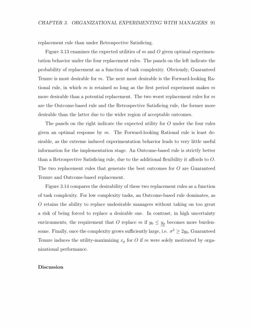
CHAPTER 3. ORGANIZATIONAL EXPERIMENTING WITH MANAGERS 91
replacement rule than under Retrospective Satisficing.
Figure 3.13 examines the expected utilities of m and O given optimal experimen-
tation behavior under the four replacement rules. The panels on the left indicate the
probability of replacement as a function of task complexity. Obviously, Guaranteed
Tenure is most desirable for m. The next most desirable is the Forward-looking Ra-
tional rule, in which m is retained so long as the first period experiment makes m
more desirable than a potential replacement. The two worst replacement rules for m
are the Outcome-based rule and the Retrospective Satisficing rule, the former more
desirable than the latter due to the wider region of acceptable outcomes.
The panels on the right indicate the expected utility for O under the four rules
given an optimal response by m. The Forward-looking Rational rule is least de-
sirable, as the extreme induced experimentation behavior leads to very little useful
information for the implementation stage. An Outcome-based rule is strictly better
than a Retrospective Satisficing rule, due to the additional flexibility it affords to O.
The two replacement rules that generate the best outcomes for O are Guaranteed
Tenure and Outcome-based replacement.
Figure 3.14 compares the desirability of these two replacement rules as a function
of task complexity. For low complexity tasks, an Outcome-based rule dominates, as
O retains the ability to replace undesirable managers without taking on too great
a risk of being forced to replace a desirable one. In contrast, in high uncertainty
environments, the requirement that O replace m if y0 yp becomes more burden-
some. Finally, once the complexity grows sufficiently large, i.e. �2 � 2y0, Guaranteed
Tenure induces the utility-maximizing xp for O if m were solely motivated by orga-
nizational performance.
Discussion
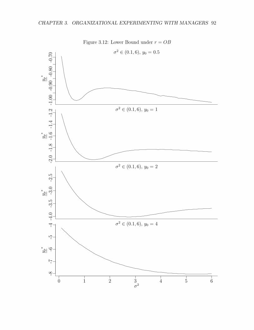
CHAPTER 3. ORGANIZATIONAL EXPERIMENTING WITH MANAGERS 92
Figure 3.12: Lower Bound under r = OB
s2
y p⇤
-1.0
0-0
.90
-0.8
0-0
.70 �2 2 (0.1, 6), y0 = 0.5
s2
y p⇤
-2.0
-1.8
-1.6
-1.4
-1.2 �2 2 (0.1, 6), y0 = 1
s2
y p⇤
-4.0
-3.5
-3.0
-2.5
�2 2 (0.1, 6), y0 = 2
s2
y p⇤
-8-7
-6-5
-4 �2 2 (0.1, 6), y0 = 4
0 1 2 3 4 5 6�2
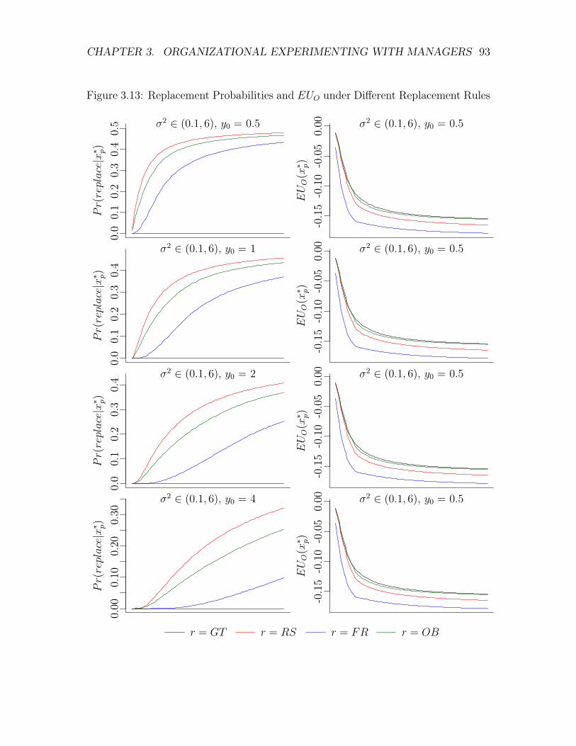
CHAPTER 3. ORGANIZATIONAL EXPERIMENTING WITH MANAGERS 93
Figure 3.13: Replacement Probabilities and EUO under Different Replacement Rules
s2
Pr(replace|x
⇤ p)
0.0
0.1
0.2
0.3
0.4
0.5 �2 2 (0.1, 6), y0 = 0.5
s2
Pr(replace|x
⇤ p)
0.0
0.1
0.2
0.3
0.4
�2 2 (0.1, 6), y0 = 1
s2
Pr(replace|x
⇤ p)
0.0
0.1
0.2
0.3
0.4 �2 2 (0.1, 6), y0 = 2
s2
Pr(replace|x
⇤ p)
0.00
0.10
0.20
0.30
�2 2 (0.1, 6), y0 = 4
s2
EUO(x⇤ p)
-0.1
5-0
.10
-0.0
50.
00 �2 2 (0.1, 6), y0 = 0.5
s2
EUO(x⇤ p)
-0.1
5-0
.10
-0.0
50.
00 �2 2 (0.1, 6), y0 = 0.5
s2
EUO(x⇤ p)
-0.1
5-0
.10
-0.0
50.
00 �2 2 (0.1, 6), y0 = 0.5
s2
EUO(x⇤ p)
-0.1
5-0
.10
-0.0
50.
00 �2 2 (0.1, 6), y0 = 0.5
r = GT r = RS r = FR r = OB

CHAPTER 3. ORGANIZATIONAL EXPERIMENTING WITH MANAGERS 94
Figure 3.14: Comparing Guaranteed Tenure and Outcome-based Replacement
s2
EUO(GT)�
EUO(OB)
-0.0
040.
000
0.00
4�2 2 (0.1, 6), y0 = 0.5
s2
EUO(GT)�EUO(OB)
-0.0
20.
000.
010.
02
�2 2 (0.1, 6), y0 = 1
s2
EUO(GT)�
EUO(OB)
-0.0
50.
000.
05
�2 2 (0.1, 6), y0 = 2
s2
EUO(GT)�
EUO(OB)
-0.3
-0.2
-0.1
0.0
0.1 �2 2 (0.1, 6), y0 = 4
0 1 2 3 4 5 6�2
CHAPTER 3. ORGANIZATIONAL EXPERIMENTING WITH MANAGERS 95
Recent management scholarship emphasizes the desirability of experimental pro-
totyping and evidence-based management as a way to improve organizational per-
formance. While it is true that offline experimentation can help organizations avoid
making strategic errors and also encourage exploratory search, the conflicting moti-
vations of managers can sap offline experiments of their informational value. Career
concerns of managers, in particular, may lead to overly exploitative prototyping
behavior and may lead to over-exploratory prototyping behavior, depending on how
organizations evaluate their managers. When managerial competence or effectiveness
with a task is measured relative to an organization’s prior performance, managers
tend to be overly incremental in their experimentation behavior. In contrast, when
managers are judged based on their capacity to implement a more desirable online
change than an unexperienced replacement, managers tend to be overly exploratory.
I evaluate two mechanisms that organizations can use to ameliorate this agency
problem. Guaranteed tenure alleviates the career concerns of managers by ensuring
that they will keep their jobs notwithstanding the desirability of their experimen-
tal prototype. Guaranteed tenure also requires that organizations sometimes keep
managers who the organization believes to be a poor fit. An outcome-based re-
placement rule induces managers to create the prototype that the organization finds
most desirable, but requires that organizations sometimes replace managers who are
likely to produce high quality organizational outcomes. The paper shows that the
freedom afforded by guaranteed tenure leads to better organizational performance
in high complexity task environments. The organizational control exerted by the
outcome-based rule, in contrast, is more desirable in low uncertainty environments.
Chapter 4
Social Movements as Purveyors of
Legislative Expertise
Introduction
For the last two decades, a major emphasis in sociological research on social
movements has been demonstrating the impact of social movements on the policy
process. Scholars have found empirical support for the power of movements in a
variety of policy domains, including civil rights, women’s rights, environmental pro-
tection, medicine, lesbian and gay rights, and antiwar (Amenta et al., 2010). In
recent years, scholars have added nuance to this basic finding by demonstrating the
stages of the policy process wherein movements matter most (e.g. Soule and King,
2006) and by demonstrating that the effect of movements on the policy process is
often contingent on facets of the political environment (e.g. Soule and Olzak, 2004).
At the core of this literature is the idea that social movements matter to the policy
process because they transmit valuable information to legislators (Gillion, 2013).
For example, large public protests send a signal to lawmakers about the interests
96
CHAPTER 4. SOCIAL MOVEMENTS AND LEGISLATIVE EXPERTISE 97
and level of commitment of constituents. Similarly, letter-writing campaigns can
demonstrate the breadth of support for a previously overlooked legislative matter
(e.g. Gillion, 2013; Lohmann, 1993). By providing informative signals to lawmakers
about constituent preferences and priorities, the activities of social movements can
move certain issues up the legislative agenda and create opportunities for novel issues
to gain legislative attention (Soule and King, 2006). Baumgartner and Jones (2015)
describe this type of information as entropic information, because it helps to bring
order to the chaotic set of problems and interests that make up the legislative process.
Baumgartner and Jones (2015) also identify a second class of information that
is equally important to the legislative process, but which has received considerably
less attention in the social movements literature: expert information. While entropic
information helps lawmakers decide what issues are important to their constituents,
expert information helps legislators design policies that achieve desired goals. Once
a problem has been identified and the legislature sets out to write new legislation,
lawmakers rely on organizations and individuals with expertise to help them craft an
appropriate solution (Bendor and Meirowitz, 2004; Callander, 2008; Esterling, 2004).
External experts also lend credibility to the policy process by making legislative
outcomes appear to be the product of rational deliberation (Epstein, 1996; Nelkin,
1975).
Social movements and, in particular, social movement organizations (SMOs), have
increasingly become sources of policy expertise, particularly for legislative issues re-
lated to the environment and public health (Andrews, 2006; Bosso, 2005; Burstein
and Hirsh, 2007; Epstein, 1996; Shaiko, 1999). Their expertise gains them access
to and influence over the policy process. Congressional committees often design
consequential, highly technical legislation with short timelines for consideration and
limited internal subject-matter expertise (Hall and Deardorff, 2006; Weiss, 1992).
CHAPTER 4. SOCIAL MOVEMENTS AND LEGISLATIVE EXPERTISE 98
As a result, SMOs, think tanks, and other interest organizations are invited into the
policy process in order to help lawmakers with legislative research, policy communi-
cation, and even drafting legislative language (Baumgartner and Leech, 1998; Berry,
1977; Heinz et al., 1993; Morales, 2013; Schlozman and Tierney, 1986). In addition
to extensive work behind-the-scenes, SMOs and other interest organizations are also
frequently invited to publicly testify before Congress on pending pieces of legislation
(Andrews and Edwards, 2004; Burstein and Hirsh, 2007).
Entropic information and expert information are relevant at different moments in
the legislative process (Baumgartner and Jones, 2015). Entropic information is most
important when the legislature is searching for new items to place on the agenda
or prioritizing the pressing matters before the Congress. Organizations that can
convincingly signal the breadth and strength of constituent preferences, therefore,
should have outsized access to the policy process early in the agenda-setting phase
(Baumgartner and Jones, 2009; Kingdon, 1984). Expert information, in contrast,
is valuable once the Congress has focused on a particular legislative matter and is
in the process of selecting a policy instrument. For legislative issues nearing votes
in committee or on the floor of the House or Senate, therefore, organizations with
expertise should have privileged access to the policy process.
In our paper, we examine patterns of access to the legislative process for en-
vironmental social movement organizations (EMOs). In addition to engaging in
outsider activism, the environmental movement has actively sought to legitimate its
policy claims and influence skeptical policymakers through the development of scien-
tific knowledge (Andrews and Edwards, 2004; Andrews, 2006; Hadden, 2015; Rome,
2013). Further, the uncertainty and complexity associated with environmental poli-
cymaking creates opportunities for EMOs to use their internal expertise in order to
exercise informational influence on the policy process (Allen et al., 2001; Eden, 1998;
CHAPTER 4. SOCIAL MOVEMENTS AND LEGISLATIVE EXPERTISE 99
Farber, 2003; Stone, 1993). As a result, the environmental movement is a valuable
place to begin an examination of how SMOs utilize scientific expertise in order to
gain access to the policy process.
In our study, we use invitations to testify before Congress as an indication that
an EMO has been given access to the policy process. We then use the characteristics
of the hearings to which the organizations are invited in order to learn when in the
policy process EMOs are most influential. Finally, we compare the observed patterns
of EMO testimony against what we observe for other interest organizations that lack
environmental expertise.
We find that EMOs have privileged access to the legislative process when com-
mittees are considering specific pieces of environmental legislation. EMOs and non-
environmental interest groups are invited to testify before Congress in roughly equal
numbers during exploratory, investigatory, or oversight hearings. However, EMO
representation at congressional hearings increases once a congressional committee is
in deliberations over legislative language, and by a significantly greater amount than
non-environmental interest organizations.
We conclude that the role of SMOs as providers of expert information to the pol-
icy process is important, but under-examined in the social movements literature. The
provision of expert information is a key avenue through which SMOs can generate
access to elite actors, which has previously been identified as important to successful
policy outcomes (Amenta et al., 1992, 1994; Cress and Snow, 2000; Soule and King,
2006). Further, we demonstrate how SMOs with expertise have the opportunity to
influence legislation at a fairly advanced stage in the policy process (King et al.,
2007, 2005; Olzak and Soule, 2009; Soule and King, 2006).
Theory and Hypotheses
CHAPTER 4. SOCIAL MOVEMENTS AND LEGISLATIVE EXPERTISE 100
The existing literature identifies two primary mechanisms for how social move-
ments impact the policy process (see e.g. Andrews and Edwards, 2004). The first
points to the signals that protests send to legislators and other important interests.
The second centers on the way social movement organizations gain access to and
allies within the legislature. Our paper focuses primarily on the second of these
mechanisms, but we briefly describe the first.
Protest Signals and Legislative Response
Many researchers argue that social movements impact legislators because they
send important informational signals about constituents’ views on issues (e.g. An-
drews and Edwards, 2004; Gillion, 2012, 2013; Lohmann, 1993). As Lohmann (1993,
p. 320) notes, protest “informs the political leader’s decisions and thus affects policy
outcomes.” This idea is embedded in the democratic theory of politics, which asserts
that electoral incentives align the legislative decisions of officeholders with the pref-
erences of the majority of their constituency (e.g. Downs, 1957; Erikson et al., 2002;
Page and Shapiro, 1983; Soule and Olzak, 2004). The activities of social movements,
much like public opinion polls, serve as a gauge of constituents’ preferences on a
given issue.
Much of the sociological work on signaling focuses on public protest, rather than
other activities that social movements engage in, because public protest is one of the
most visible activities social movements undertake (Kollman, 1998; Lipsky, 1968).
This existing work examines several facets of protest that make it more worthy of
congressional attention, such as the frequency or the size of protest events (e.g.
Agnone, 2007; Burstein and Freudenburg, 1978; DeNardo, 1985; King et al., 2007;
Lohmann, 1993; McAdam and Su, 2002; Olzak and Soule, 2009; Santoro, 2002, 2008).
To the extent that the signal sent by protest is perceived to reflect the interests of
CHAPTER 4. SOCIAL MOVEMENTS AND LEGISLATIVE EXPERTISE 101
the voting public, legislators will react with policy decisions that are in line with
the protest’s demands (Gillion, 2013). In addition to the direct impact of protest
on legislators, the literature also argues that protest sends signals to bystander con-
stituents, who may either join the movement or pressure legislators in other ways
(Andrews and Edwards, 2004; Giugni, 2004; Jenkins, 1987; Lipsky, 1968). Protest is
powerful because it can threaten legislators directly, or do so indirectly by its impact
on the opinions, values, and beliefs of other important constituencies.
Social Movement Organizations and Legislative Response
In addition to the signaling mechanism of protest, some movement scholars argue
that another important mechanism of movement legislative influence is via social
movement organizations’ ability to gain access to the legislative process or mobilize
allies in Congress (Amenta et al., 2010; Andrews and Edwards, 2004; Kane, 2003;
King et al., 2007; McCammon et al., 2001; Olzak and Soule, 2009; Soule et al., 1999;
Soule, 2004; Soule and Olzak, 2004). Elite allies, in turn, can act as a mouthpiece for
a social movement within the government, provide an avenue for social movement
organizations to get access to the legislative process, and ensure that the issues pro-
moted by the social movement receive favorable placement on the legislative agenda
(Amenta et al., 1992, 1994; Cress and Snow, 2000; Soule and King, 2006).
The empirical literature on the impact of movement organizations on legislators
has established a correlation between the density (i.e., number) of social movement
organizations in a given location (i.e., city, state, or nation) and the passage of leg-
islation favorable to the movement in question. For example, Soule et al. (1999)
find a correlation between the number of feminist SMOs and roll call votes and con-
gressional hearings on women’s issues (for similar findings, see Johnson et al., 2010;
CHAPTER 4. SOCIAL MOVEMENTS AND LEGISLATIVE EXPERTISE 102
Kane, 2003; Olzak and Soule, 2009; Soule, 2004). This literature has also estab-
lished a correlation between the use of certain tactics mainly associated with social
movement organizations and policymaking around the movement in question. For
example, Soule et al. (1999) find a correlation between the mention of letter-writing,
petitions, and lobbying in news accounts of feminist protest and congressional hear-
ings and roll call votes on women’s issues (for similar findings, see McCammon et al.,
2001; Olzak and Soule, 2009).
This empirical work is important because it suggests that social movement or-
ganizations likely influence legislation in some way. However, the literature thus far
lacks a nuanced understanding of what exactly it is that movement organizations do
to produce these responses from policymakers. We argue that providing information
and expertise to legislators is an important but largely underexamined mechanism
of movement influence on policy (Burstein and Hirsh, 2007, is an important excep-
tion). Like other actors in the “policy community or subsystem” of government, such
as bureaucrats, researchers, and other interest groups (Sabatier, 1991), social move-
ment organizations help to draft legislation, testify at hearings, and present research
(e.g. Berry, 1977; Heinz et al., 1993; Schlozman and Tierney, 1986). We develop this
argument in the next section.
Expert Information and the Legislative Process
There are two kinds of information that are relevant to the impact of social
movements on policy. The first, entropic information, is critical to the search stage
of policy, when legislators are deciding the issues upon which to focus their attention
(Baumgartner and Jones, 2015). The second kind of information relevant to the
impact of movements on policy, and the focus of this paper, is expert information.
The policy outcomes of proposed bills are often difficult to predict beforehand,
CHAPTER 4. SOCIAL MOVEMENTS AND LEGISLATIVE EXPERTISE 103
and may interact with existing legislation in unexpected ways. Thus, legislators
rely on expert information in order to ensure that the policy outcomes of a piece of
legislation reflect the intended policy goals (Baumgartner and Jones, 2015; Callander,
2008; Esterling, 2004). Furthermore, gaining public support for legislative initiatives
requires convincing the public that a new bill will benefit their interests. Legislation
that is well justified at the outset can calm the concerns of a mistrustful electorate
(Cobb and Kuklinski, 1997; Esterling, 2004). Finally, a norm of scientific rationalism
pervades legislative debate. Legislators and the public often insist that a policy has
a scientifically supported basis for implementation (Ezrahi, 1990; Habermas, 1971;
Nelkin, 1975).
In order to write legislation that reflects the policy goals of informed lawmakers,
the Congress created the committee system in order to ensure that Members develop
expertise on issues of interest. Each committee is endowed with exclusive jurisdic-
tion over a piece of the legislative agenda (King, 1994, 1997; Krehbiel, 1991; Smith
and Deering, 1997). Committee members are expected to become resident experts
in their assigned areas of jurisdiction (Cooper, 1970; Gilligan and Krehbiel, 1987,
1990; Krehbiel, 1991, 2004). As a result, the task of writing important legislation is
commonly delegated to committee leadership in conjunction with other committee
members. Further, if a new piece of legislation originates outside of the committee
with jurisdiction, the congressional leadership refers it to the relevant committee.
Committees then have the option to edit the legislation and report it back to the
full legislative body for consideration. Committee specialization gives the legislature
confidence that the lawmakers who are perceived to be most knowledgeable have first
reviewed all the bills that receive consideration by the full House or Senate (Krehbiel,
1991; Shepsle and Weingast, 1987; Smith and Deering, 1997).

CHAPTER 4. SOCIAL MOVEMENTS AND LEGISLATIVE EXPERTISE 104
Committee members and their staffs rely on other entities for information on is-
sues that require significant scientific or technical expertise. Despite the considerable
resources that exist in the executive agencies, the legislative branch often chooses in-
stead to seek expertise elsewhere in order to protect its independence and circumvent
potential political conflicts between the legislative and executive branches (Brudnick,
2011; Weiss, 1992). For some policy questions, committees can find sufficient exper-
tise within the legislative branch, in particular through the Congressional Research
Service, which acts as an internal think-tank for legislators and their staffs. How-
ever, committees work on short and unpredictable time schedules. The 600-person
Congressional Research Service is often overtaxed with requests and lacks necessary
specialized knowledge to answer many questions (Kosar, 2015). As a result, commit-
tees often look beyond the legislative branch for policy expertise (Hall and Deardorff,
2006; Hansen, 1991; Wright, 1995).
Interest organizations, think tanks, and advocacy groups make themselves avail-
able to assist Members of Congress and their staffs in need of answers to important
legislative questions (Wright, 1995). These extra-governmental organizations aspire
to become trusted resources for legislative committees in order to gain influence over
the design of policy proposals. Legislators know that the information offered by in-
terest organizations comes from a biased perspective. But, for interest organizations
with policy goals that are sufficiently aligned with the lawmaker’s and for issues
around which there is significant policy uncertainty, legislators are willing to rely on
this information in order to ameliorate the risk of unintended outcomes. This legisla-
tive bias-variance trade off leads to policy outcomes that are better aligned with the
preferences of the interest organization than would be predicted by the preferences
of the median legislator (Bendor and Meirowitz, 2004; Callander, 2008; Gilligan and
Krehbiel, 1987; Krehbiel, 1991; Wright, 1995).
CHAPTER 4. SOCIAL MOVEMENTS AND LEGISLATIVE EXPERTISE 105
Social movement organizations are well suited to provide expert information and
take advantage of informational influence. Social movements have long relied on sci-
entific knowledge as a tool to support their organizational goals (Brown et al., 2004;
Epstein, 1996; Ezrahi, 1990; Habermas, 1971; Johnson, 2006; Rome, 2013). Social
movements often have mature networks of experts willing to aid in their causes.
The environmental movement has been particularly effective at engaging environ-
mental scientists in order to justify legislative efforts on species protection, forest
preservation, and emissions reduction (Bosso, 2005; Shaiko, 1999). Recent move-
ments have also demonstrated the ability to work within the scientific community
to generate new scientific knowledge in order to justify claims or refute opponents’
claims (Brown et al., 2004; Epstein, 1996; Jamison, 2001; Rome, 2013). Further,
the public views social movement organizations differently than corporate lobbyists
and business groups. Social movement organizations are perceived as more trust-
worthy advocates for the public interest than corporations or, for that matter, the
government (Edelman, 2015; Lyon and Maxwell, 2008; Soule, 2009). Therefore, by
partnering with a social movement organization, legislators may be able to secure
broader political support for a legislative initiative.
Congressional Committees and Information Collection
Empirical examination of which organizations provide expert information to pol-
icymakers and committee staffs is complicated by the informal nature of the rela-
tionships between the Congress and interest organizations. Private meetings, phone
calls, and e-mail exchanges between Members, their staffs, and representatives of in-
terested parties occur daily. Because the Congress is exempt from keeping workplace
records and Freedom of Information Act requests, systematic data on expert access
is challenging to collect.
CHAPTER 4. SOCIAL MOVEMENTS AND LEGISLATIVE EXPERTISE 106
However, interviews by the authors indicate that examining which organizations
testify at congressional hearings provides an accurate picture of the organizations
that are most influential on a legislative topic. Staff members often invite testi-
mony from the organizations that they have worked with in private. Furthermore,
staff preparation for a hearing often involves lengthy conversations with prospective
witnesses. According to an employee at a prominent environmental advocacy orga-
nization: “If you’ve been working closely with [a committee] on legislation and then
[the committee has] a hearing related to it, they’re going to want to bring the people
that know the most about the issue they’re working on.”
Hearings provide an institutionalized, public avenue for committees to seek expert
information. The Congress holds thousands of public hearings every year. A hearing
can include as little as a single witness and as many as a few dozen witnesses. In
addition to movement organizations, other interest organizations are commonly in-
vited to testify (e.g., labor unions, trade associations and industry groups). Affected
parties may be called in order to offer a real-world perspective or to demonstrate how
a proposed legislative change would impact a key constituency. For technical or com-
plex policy questions, academic researchers may be called to testify, as well. Finally,
it is not unusual for other government officials to testify at hearings, particularly
when the topic under consideration cuts across jurisdictional lines (Baumgartner
and Jones, 2015; Burstein and Hirsh, 2007; Leyden, 1995; Talbert et al., 1995).
Hearings are one part theatrical puffery and one part legislative substance. Hear-
ings serve as an opportunity for lawmakers to get media attention and to demonstrate
issue knowledge to constituents. Hearings are carefully designed to elicit testimony
to support the interests of the majority party. Question-and-answer sessions are of-
ten scripted, with each Member assigned particular questions to elicit predetermined
responses (Leyden, 1995; Oleszek, 1989). Yet, the ceremonial aspects of hearings
CHAPTER 4. SOCIAL MOVEMENTS AND LEGISLATIVE EXPERTISE 107
should not belie their legislative role. The process of hearing preparation provides
deadlines for staff and substantive education for lawmakers. Organizations invited
to testify often create detailed reports and white papers to support submitted testi-
mony. Finally, although some hearings receive a great deal of media attention, and a
few are even televised live, even lightly publicized hearings are often important events
for affected constituencies (Baumgartner and Jones, 2015; Burstein and Hirsh, 2007;
Diermeier and Feddersen, 2000; Oleszek, 1989).
The content of a particular hearing provides information about the stage in the
legislative process when an organization is given access. There are two broad classes
of congressional hearings: non-legislative and legislative. Non-legislative hearings are
not tied to a specific bill and may focus on virtually any topic deemed important by
a committee (Talbert et al., 1995). Two common types of non-legislative hearings
are investigatory and oversight hearings, which usually examine the efficacy of a
federal program or potential wrongdoing by a private company or government official.
Non-legislative hearings can also be called for the purpose of raising the profile of
a legislative issue, to demonstrate responsiveness to important constituents, or to
publicly claim jurisdiction over an issue or set of issues. The decision to hold a non-
legislative hearing indicates that an issue is in a preliminary stage in the legislative
process.
Legislative hearings, in contrast, are tied to a specific bill that may become law.
Legislative hearings are called after a bill has been introduced by a Member and
referred to a committee (Baumgartner and Jones, 2015; Talbert et al., 1995). The
decision to hold a legislative hearing indicates that a committee is seriously consid-
ering referring a bill to the full legislative body. A committee will hold legislative
hearings just prior to the bill “markup.” During markup, the committee members
submit amendments to a bill under consideration and then vote on whether to send
CHAPTER 4. SOCIAL MOVEMENTS AND LEGISLATIVE EXPERTISE 108
the amended bill back to the full legislature (Koempel and Schneider, 2007; Sachs,
2003; Smith and Deering, 1997).
Hypotheses
Given the above discussion, we develop two core hypotheses about EMO access
to the legislative process. First, we predict that EMOs will have greater access to
the legislative process as a bill reaches a more advanced stage within the committee.
During the search phase of the policy process, the committee seeks information from
a broad set of interests with diverse areas of knowledge. In contrast, once a com-
mittee has decided to put forth new legislation to the full Congress, the committee
seeks specialists with subject area expertise. Therefore, we expect that the number
of EMOs invited to testify at hearings that are explicitly tied to the design of a piece
of environmental protection legislation will exceed the number of EMOs in hearings
related to environmental protection that are non-legislative.
H1: More EMOs are invited to testify at legislative hearings than non-legislative hear-
ings.
We would not predict this same pattern to hold for interest organizations that
lack environmental expertise. During the search phase, we expect the legislature to
invite other interest organizations with strong preferences on environmental protec-
tion to testify alongside EMOs. Once a committee’s agenda is determined and a
particular piece of legislation is under consideration, we expect that the committee
will be more discerning. Only those organizations with specific expertise and, likely,
with whom the committee has a prior relationship, will be invited to testify. As a
result, we expect that the increase in representation for EMOs will exceed the change
CHAPTER 4. SOCIAL MOVEMENTS AND LEGISLATIVE EXPERTISE 109
in representation for non-environmental interest organizations.
H2: The increase in EMO representation will exceed the increase in representation of
non-environmental interest organizations across non-legislative and legislative hear-
ings.
Empirical Setting: The Environmental Movement in the United States
We examine the participation of environmental movement organizations in envi-
ronmental protection hearings. We collect data on congressional hearings related to
species and forestry protection from 1988 to 2007. We choose species and forestry
issues because these are traditionally at the nexus of environmental activism and
environmental science.
Data
We collect data on every congressional hearing held on “species and forest pro-
tection” in the U.S. House of Representatives over 10 Congresses from 1988 (100th)
through 2007 (109th). We use the Policy Agendas Project coding scheme to identify
the relevant hearings. From these data on hearings, we code several relevant pieces of
information. First, we utilize the classification scheme created by the Policy Agendas
Project to determine whether a hearing was legislative or non-legislative in nature.
The Policy Agendas Project classifies hearings as legislative if they mention a bill
number or name explicitly in the title of the hearing. The hearing is classified as
non-legislative if there is no bill number or bill name indicated (Talbert et al., 1995).
In all, there were 276 hearings during this period. 122 were legislative and 154 were
non-legislative.
Next, we examine the organizational affiliations of each of the witnesses invited
CHAPTER 4. SOCIAL MOVEMENTS AND LEGISLATIVE EXPERTISE 110
to testify at each of these 276 hearings. We collected and transcribed the organiza-
tional affiliation of each witness using the ProQuest Congressional Hearing Digital
Collection. In all, we obtained a list of 2,611 witnesses at the 276 environmental
hearings in this time period. These witnesses were affiliated with 1,019 different
organizations. Once we had this list of 1,019 organizations, we coded each by orga-
nizational type. We researched each organization using the organization’s website
and/or in other public materials about the organization (e.g., newspaper articles,
research articles, etc.). For defunct organizations, we also used the Way Back Ma-
chine (http://archive.org/web/) to find archived websites. We found information on
950 of the organizations that testified. We created three organizational categories:
(1) environmental movement organization (n=153); (2) non-environmental interest
organization (n=182); (3) not interest organization (n=615).
We coded an organization as an EMO if on its website or other public materials
it was stated that the organization’s primary purpose is environmental protection
and indicates that the organization publicly agitates for environmental protection.
We did not distinguish between organizations based on particular policy positions.
Most supported environmental conservation for its own end (e.g., Wilderness Society,
Sierra Club). Some, however, supported preservation for the purposes of recreation,
hunting, or fishing (e.g., U.S. Sportsmen’s Alliance, Safari Club International). We
categorized regional chapters of organizations by their national organizing group
(e.g., the Hawaii Audubon Society was grouped with the National Audubon Society).
We identified 153 of the organizations as EMOs.
We coded an organization as a non-environmental interest organization if the or-
ganization’s goals were not primarily environmental and a stated method for achiev-
ing its organizational goals was government influence (see Burstein, 1998; Walker,
CHAPTER 4. SOCIAL MOVEMENTS AND LEGISLATIVE EXPERTISE 111
1991; Wilson, 1973). Labor unions, professional associations, and local civic organi-
zations were coded as non-environmental interest organizations. Although the prefer-
ences of a non-environmental interest organization may align with the environmental
movement on a particular legislative issue, we attempted to categorize organizations
based on their stated organizational mission. Therefore, all organizations that ex-
plicitly represent commercial hunters, commercial fishermen, forest industries, and
companies that manufacture or sell recreational products were categorized in this
group. Organizations that publicly supported environmental protection, but whose
membership consisted exclusively of industry interests were grouped in this category
as well. We identified 182 of the organizations as non-environmental interest groups.
All other organizations were classified as “not interest organization.” These in-
clude government and quasi-governmental organizations, think tanks, for-profit cor-
porations, and universities. Zoos, aquariums, and circuses were coded in this cat-
egory, as well. (However, organizations involved in animal conservation that also
manage zoos or aquariums, such as the Wildlife Conservation Society, were coded as
EMOs). The remaining 615 organizations were classified to be in this category.
We also collect a series of variables about hearings that we use as controls in our
regression analyses. These include the committee that is holding the hearing, the
two-year Congress in which the hearing takes place, and the number of sessions in
the hearing. Consistent with the Policy Agendas Project, we also note whether the
hearing was related to appropriations, the creation of a new government agency, or
legislation proposed by the President. We control for the length of the hearing in case
legislative hearings and non-legislative hearings tend to have a different number of
witnesses. We control for the committee holding the hearing, the Congress in which
the hearing takes place, and the type of hearing to ensure that our estimates are not
being driven by a single committee, single Congress, or single type of hearing. Note
CHAPTER 4. SOCIAL MOVEMENTS AND LEGISLATIVE EXPERTISE 112
that by controlling for the two-year Congress, we implicitly also control for partisan
control of the Congress.
Analysis and Results
We begin by examining whether more EMOs are invited to testify in legislative
hearings than non-legislative hearings. We find that legislative hearings do tend
to include more EMOs than non-legislative hearings. The average non-legislative
hearing includes testimony from 1.21 EMOs, compared with 1.95 EMO participants
at legislative hearings. A Welch Two-Sample T-Test indicates that this difference is
significant at the 99% level.
We test this relationship using a series of regression analyses, which allow us to
control for potential alternative explanations. We use negative binomial regression,
which is common for modeling count data in the presence of overdispersion. We
estimate the model using the “glm.nb” command in R 3.1.0.
The results are presented in Table 4.1. The first model predicts the number of
EMOs invited to testify at each hearing, after controlling for the two-year Congress,
the length of the hearing, the congressional committee that called the hearing,
whether the hearing was related to appropriations, the creation of a new agency,
or in response to a Presidential proposal. We then add an indicator variable for
whether the hearing was legislative in nature. The coefficient on this variable is
positive and significant, which is consistent with our theory.
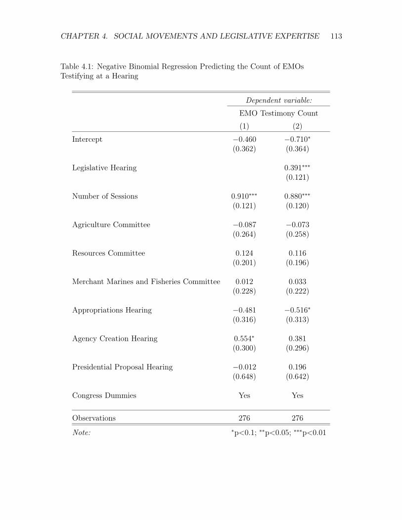
CHAPTER 4. SOCIAL MOVEMENTS AND LEGISLATIVE EXPERTISE 113
Table 4.1: Negative Binomial Regression Predicting the Count of EMOsTestifying at a Hearing
Dependent variable:EMO Testimony Count(1) (2)
Intercept �0.460 �0.710⇤(0.362) (0.364)
Legislative Hearing 0.391⇤⇤⇤(0.121)
Number of Sessions 0.910⇤⇤⇤ 0.880⇤⇤⇤(0.121) (0.120)
Agriculture Committee �0.087 �0.073(0.264) (0.258)
Resources Committee 0.124 0.116(0.201) (0.196)
Merchant Marines and Fisheries Committee 0.012 0.033(0.228) (0.222)
Appropriations Hearing �0.481 �0.516⇤(0.316) (0.313)
Agency Creation Hearing 0.554⇤ 0.381(0.300) (0.296)
Presidential Proposal Hearing �0.012 0.196(0.648) (0.642)
Congress Dummies Yes Yes
Observations 276 276
Note: ⇤p<0.1; ⇤⇤p<0.05; ⇤⇤⇤p<0.01
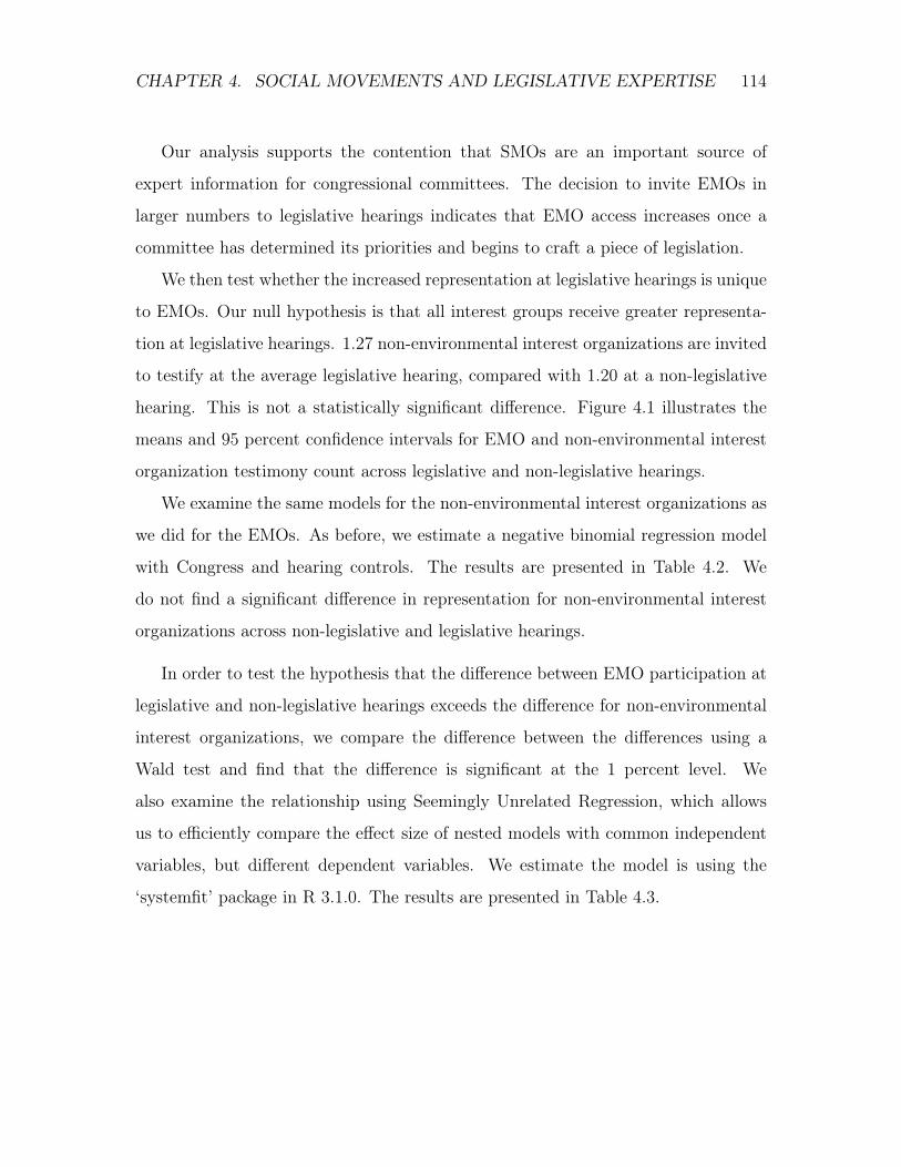
CHAPTER 4. SOCIAL MOVEMENTS AND LEGISLATIVE EXPERTISE 114
Our analysis supports the contention that SMOs are an important source of
expert information for congressional committees. The decision to invite EMOs in
larger numbers to legislative hearings indicates that EMO access increases once a
committee has determined its priorities and begins to craft a piece of legislation.
We then test whether the increased representation at legislative hearings is unique
to EMOs. Our null hypothesis is that all interest groups receive greater representa-
tion at legislative hearings. 1.27 non-environmental interest organizations are invited
to testify at the average legislative hearing, compared with 1.20 at a non-legislative
hearing. This is not a statistically significant difference. Figure 4.1 illustrates the
means and 95 percent confidence intervals for EMO and non-environmental interest
organization testimony count across legislative and non-legislative hearings.
We examine the same models for the non-environmental interest organizations as
we did for the EMOs. As before, we estimate a negative binomial regression model
with Congress and hearing controls. The results are presented in Table 4.2. We
do not find a significant difference in representation for non-environmental interest
organizations across non-legislative and legislative hearings.
In order to test the hypothesis that the difference between EMO participation at
legislative and non-legislative hearings exceeds the difference for non-environmental
interest organizations, we compare the difference between the differences using a
Wald test and find that the difference is significant at the 1 percent level. We
also examine the relationship using Seemingly Unrelated Regression, which allows
us to efficiently compare the effect size of nested models with common independent
variables, but different dependent variables. We estimate the model is using the
‘systemfit’ package in R 3.1.0. The results are presented in Table 4.3.
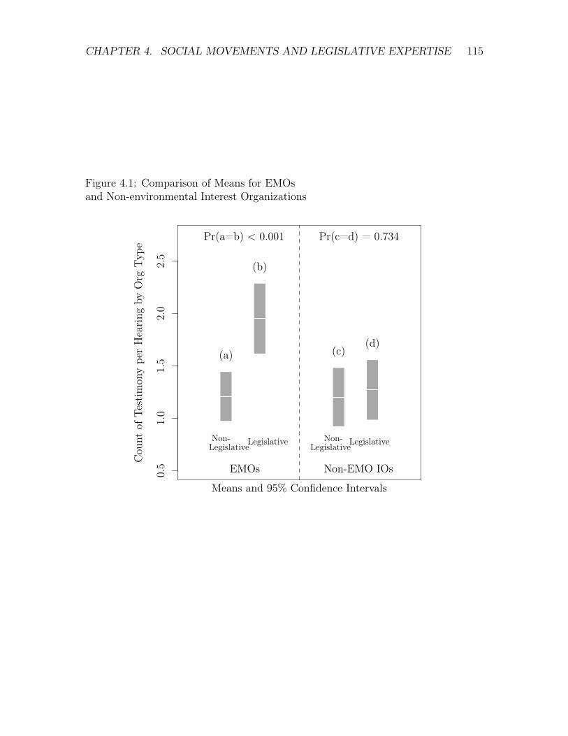
CHAPTER 4. SOCIAL MOVEMENTS AND LEGISLATIVE EXPERTISE 115
Figure 4.1: Comparison of Means for EMOsand Non-environmental Interest Organizations
Cou
ntof
Test
imon
ype
rH
earin
gby
Org
Typ
e
0.5
1.0
1.5
2.0
2.5
Means and 95% Confidence Intervals
EMOs Non-EMO IOs
Non-LegislativeLegislative Non-
LegislativeLegislative
(a)
(b)
(c)(d)
Pr(a=b) < 0.001 Pr(c=d) = 0.734
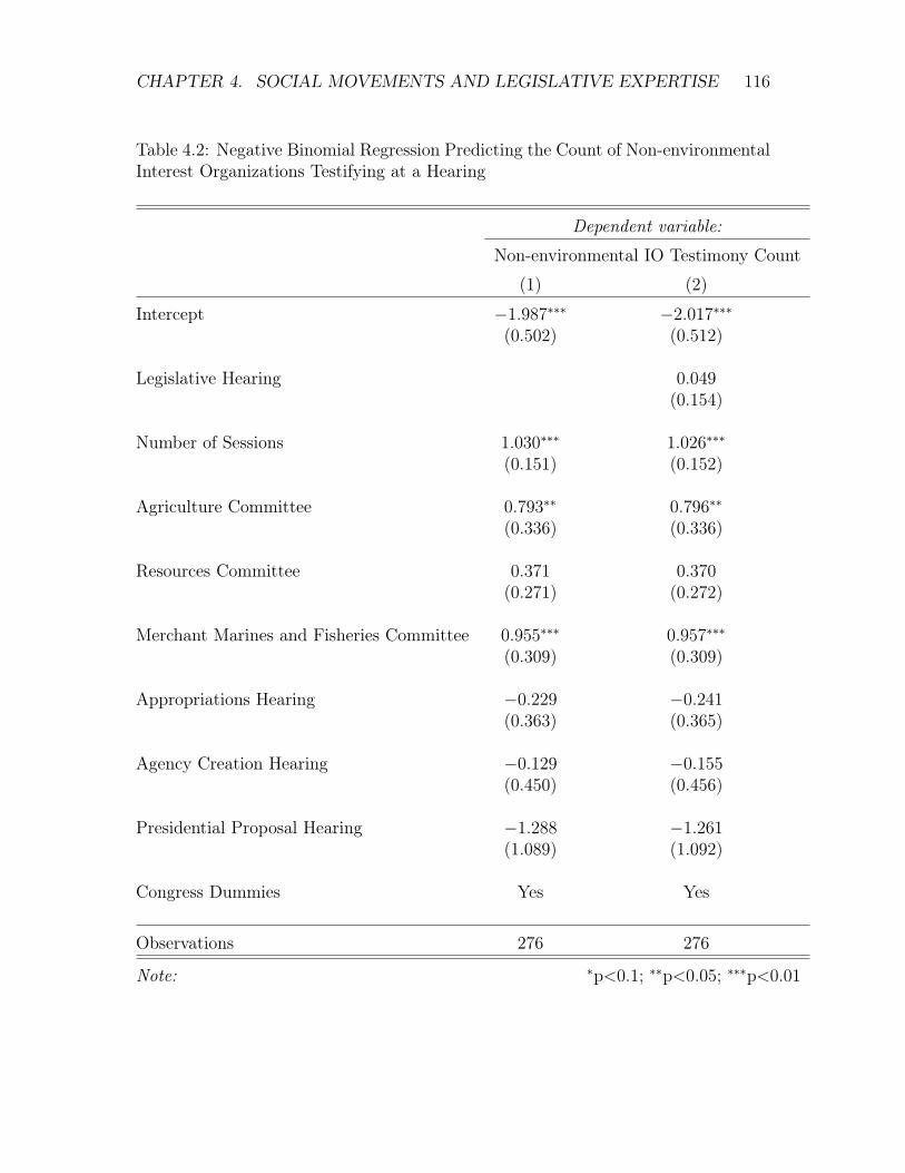
CHAPTER 4. SOCIAL MOVEMENTS AND LEGISLATIVE EXPERTISE 116
Table 4.2: Negative Binomial Regression Predicting the Count of Non-environmentalInterest Organizations Testifying at a Hearing
Dependent variable:Non-environmental IO Testimony Count
(1) (2)
Intercept �1.987⇤⇤⇤ �2.017⇤⇤⇤(0.502) (0.512)
Legislative Hearing 0.049(0.154)
Number of Sessions 1.030⇤⇤⇤ 1.026⇤⇤⇤(0.151) (0.152)
Agriculture Committee 0.793⇤⇤ 0.796⇤⇤(0.336) (0.336)
Resources Committee 0.371 0.370(0.271) (0.272)
Merchant Marines and Fisheries Committee 0.955⇤⇤⇤ 0.957⇤⇤⇤(0.309) (0.309)
Appropriations Hearing �0.229 �0.241(0.363) (0.365)
Agency Creation Hearing �0.129 �0.155(0.450) (0.456)
Presidential Proposal Hearing �1.288 �1.261(1.089) (1.092)
Congress Dummies Yes Yes
Observations 276 276
Note: ⇤p<0.1; ⇤⇤p<0.05; ⇤⇤⇤p<0.01
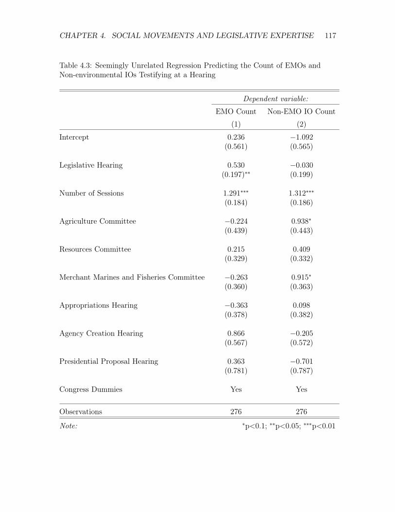
CHAPTER 4. SOCIAL MOVEMENTS AND LEGISLATIVE EXPERTISE 117
Table 4.3: Seemingly Unrelated Regression Predicting the Count of EMOs andNon-environmental IOs Testifying at a Hearing
Dependent variable:EMO Count Non-EMO IO Count
(1) (2)
Intercept 0.236 �1.092(0.561) (0.565)
Legislative Hearing 0.530 �0.030(0.197)⇤⇤ (0.199)
Number of Sessions 1.291⇤⇤⇤ 1.312⇤⇤⇤(0.184) (0.186)
Agriculture Committee �0.224 0.938⇤(0.439) (0.443)
Resources Committee 0.215 0.409(0.329) (0.332)
Merchant Marines and Fisheries Committee �0.263 0.915⇤(0.360) (0.363)
Appropriations Hearing �0.363 0.098(0.378) (0.382)
Agency Creation Hearing 0.866 �0.205(0.567) (0.572)
Presidential Proposal Hearing 0.363 �0.701(0.781) (0.787)
Congress Dummies Yes Yes
Observations 276 276
Note: ⇤p<0.1; ⇤⇤p<0.05; ⇤⇤⇤p<0.01
CHAPTER 4. SOCIAL MOVEMENTS AND LEGISLATIVE EXPERTISE 118
We then test the linear restriction that the coefficients on “Legislative Hearing”
are different across the nested models using a chi-squared test. We use the ‘linearHy-
pothesis’ command in the ‘car’ package in R 3.1.0. We find that the difference in
differences is significant at the 5 percent level.
These results provide additional evidence that SMOs are different from other
types of interest groups. Although EMOs and non-environmental interest organiza-
tions are invited in roughly equal numbers to non-legislative hearings, the increased
reliance on EMOs for expertise during legislative hearings is unique.
Conclusion and Areas for Further Research
Social movements attempting to impact the policy process seek access to elite
government actors. One way to get lawmakers to pay attention to social movement
goals is by transmitting entropic information, which is the type of information that
helps lawmakers determine their legislative priorities during each term in office. By
convincing elected officials that the movement speaks for a large and dedicated group
of voters, social protests and other forms of outsider activism are effective strategies
for utilizing the power of entropic information to increase the political influence of a
social movement.
However, social movements and SMOs also gain access to the policy process
through their organizational expertise. Lawmakers trade off a desire to achieve policy
goals with a fear of unintended consequences. Interest organizations with policy
expertise, as a result, are given privileged access to the policy process when legislation
is being crafted and debated in the legislature. Interest organizations with policy
expertise can then use this access to influence legislative outcomes. Due to their
high level of public trust and varied sources of technical knowledge, SMOs working
in scientific domains are particularly well suited to exploit expertise-based influence
CHAPTER 4. SOCIAL MOVEMENTS AND LEGISLATIVE EXPERTISE 119
on the policy process.
In our paper, we examine the patterns of EMO access to the policy process. Con-
sistent with theories of expertise-based influence, we find that EMOs get privileged
access to the legislature when congressional committees are debating specific pieces
of legislation. Further, this enhanced level of access is unique to EMOs; we do not
observe the same patterns for other interest organizations with strong opinions on
environmental regulation.
However, a crucial limitation of our paper is that we can only demonstrate leg-
islative access, not policy influence. In future work, we seek to tie expertise-based
access to concrete changes in legislative outcomes, which has been the strength of
prior work on the information-based political strategies of SMOs. We hope that
our analysis acts as a springboard for future studies that show the impact of SMO
expertise on policy outcomes, test the comparative effectiveness of expertise-based
strategies, and examine how social movements balance entropy-based and expertise-
based informational strategies to achieve their policy goals.

Appendix A
Appendix to Chapter 2
Proof of Proposition 2
I find the solution to the model using backwards induction. First, I determine
the optimal strategies for P and V conditional on reaching the proposal subgame.
Then, I determine the optimal strategies in the learning subgame, given subsequent
equilibrium strategies.
Proposal Subgame Given p(p) Not Learned
I first find the outcome of the proposal subgame, assuming that in the learning
subgame either LP= ¬L, or LP
= L and LV= ¬A.
Define the acceptance set for V , Av(p), as the set of alternatives which would be
accepted by V conditional on p. Spatially, Av(p), is the set of points in R which are
closer to 1 than p:
Av(p) =
8><
>:
[p, 2� p] if p 1
[2� p, p] if p > 1
120

APPENDIX A. APPENDIX TO CHAPTER 2 121
Define a as the alternative in Av(p) that is optimal for P to propose. If Eup(a) �
Eup(p), then PP⇤¬L = a. Otherwise, PP⇤
¬L = p.
PP⇤¬L =
8>>>>>>>><
>>>>>>>>:
a = 0 if p 0
p if 0 < p 1
a = 2� p if 1 < p 2
a = 0 if p > 2
Because the proposals are all contained in the acceptance set, Av(p), V will accept
a in equilibrium.
PV ⇤¬L = a
The expected utility for P , conditional on p, ↵, and �, and either LP= ¬L, or
LP= L and LV
= ¬A:
If PP⇤¬L is a = 0:
Eup = � [Pr( a(a) 0) |E( a(a)| a(a) 0)|+ Pr( a(a) > 0) |E( a(a)| a(a) > 0)|] =
�h12 ·
↵2� +
12 ·
↵2�
i= � ↵
2�
If PP⇤¬L = p and p 2 (0,↵]:
Eup = � [Pr( p(p) 0) |E( p(p)| p(p) 0)|+ Pr( p(p) > 0) |E( p(p)| p(p) > 0)|] =
�h⇣
�(p�↵)2↵ · p�↵
2
⌘+
�p+↵2↵ · p+↵
2
�i= �p2+↵2
2↵
If PP⇤¬L = p and p 2 (↵, 1]: Eup = �p.
If PP⇤¬L is a 2 (↵, 1): Eup = �a.
If PP⇤¬L is a 2 (0,↵]: Eup = �a+↵
2↵ .
Proposal Subgame Given p(p) Learned

APPENDIX A. APPENDIX TO CHAPTER 2 122
Next, I find the solution to the proposal subgame, assuming that LP= L and
LV= A:
V defines its acceptance set with respect to p(p) in the same way as it defined
Av(p). However, now the acceptance set is defined with respect to the learned
p(p). As a result, for p(p) near 1, there do not exist any values of a such that
Euv(a) > Euv( p(p)). There are also two sets of intermediate values, where V ’s
preference for a known p(p) over an uncertain a makes the range of Av( p(p))
smaller than the range of Av(p).
For sufficiently low p(p), V is indifferent between p(p) and a = p(p), because
p+ ↵�< 1. I find the maximum value for which V is indifferent:
p(p) +↵
�= 1
p(p) = 1� ↵
�
Therefore, for all p(p) 1� ↵�, V will accept p(p) � a � 1. By the symmetry
of V ’s utility curve, V will also accept 1 < a 2� p(p). Therefore, if p(p) 1� ↵�:
Av( p(p)) = [ p(p), 2� p(p)].
For 1 � ↵�< p(p) < 1, V prefers a known p(p) to an uncertain a. In order to
define the indifference set, I need to find the minimum and maximum a such that V

APPENDIX A. APPENDIX TO CHAPTER 2 123
is indifferent. First, I find the minimum a that satisfies:
Euv( p(p)) = Euv(a)
�(1� p(p)) = � [Pr( a(a) 1)E( a(a)| a(a) 1) + Pr(a > 1) · E( a(a)| a(a) > 1)]
1� p(p) =
1� (a� ↵
�)
2
↵�
·✓1�
1 + a� ↵�
2
◆!+
a+ ↵
�� 1
2
↵�
·✓a+ ↵
�+ 1
2
� 1
◆!
=
(a� 1)
2+ (
↵�)
2
2
↵�
a = 1�r
2(1� p(p))↵
�� (
↵
�)
2
By the same logic, the maximum a that satisfies the equality is 1+q2(1� p(p))
↵�� (
↵�)
2.
I find the minimum of the range of values of p(p) for which there does not exist
an a that V will accept by finding the values of p(p) for which the set defined above
is empty:
Find p(p) that satisfies: 1�q
2(1� p(p))↵�� (
↵�)
2= 1+
q2(1� p(p))
↵�� (
↵�)
2.q2(1� p(p))
↵�� (
↵�)
2= 0. p(p) = 1� ↵
2� .
Therefore, if p(p) 2 (1� ↵�, 1� ↵
2� ]:
Av( p(p)) = [1�q
2(1� p(p))↵�� (
↵�)
2, 1 +q2(1� p(p))
↵�� (
↵�)
2].
Further, if p(p) 2 (1� ↵2� , 1]: Av( p(p)) = ;.
By the symmetry of V ’s utility curve, I define the acceptance sets for other

APPENDIX A. APPENDIX TO CHAPTER 2 124
possible values of p(p).
Av( p(p)) =
8>>>>>>>>>>>><
>>>>>>>>>>>>:
[ p(p), 2� p(p)] if p(p) 1� ↵�
h1�
q(1� p(p))2
↵�� (
↵�)
2, 1 +q
(1� p(p))2↵�� (
↵�)
2i
if 1� ↵�< p(p) 1� ↵
2�
; if 1� ↵2� < p(p) 1 +
↵2�
h1�
q( p(p)� 1)2
↵�� (
↵�)
2, 1 +q
( p(p)� 1)2
↵�� (
↵�)
2i
if 1 + ↵2� < p(p) 1 +
↵2�
[2� p(p), p(p)] if p(p) > 1 +
↵�
As before, define a as the a 2 Av( p(p)) that is optimal for P to propose. If
Eup(a) � Eup( p(p)), then PP⇤L = a. Otherwise, PP⇤
L = p.
PP⇤L =
8>>>>>>>>>>>><
>>>>>>>>>>>>:
a = 0 if p(p) � ↵2�
p if � ↵2� < p(p) < 1 +
↵2�
a = 1�q
( p(p)� 1)2
↵�� (
↵�)
2 if 1 + ↵2� < p(p) 1 +
↵�
a = 2� p(p) if 1 + ↵�< p(p) 2
a = 0 if p(p) > 2
PV ⇤L = a
Because the proposals are all contained in the acceptance set, Av( p(p)), V will
accept in equilibrium.
The expected utility for P , conditional on p(p), ↵ and �, and LP= L and
LV= A:

APPENDIX A. APPENDIX TO CHAPTER 2 125
Eup( p(p)) =
8>>>>>>>>>>>><
>>>>>>>>>>>>:
� ↵2� if p(p) � ↵
2�
� p(p) if � ↵2� < p(p) < 1 +
↵2�
�a if 1 + ↵2� < p(p) 2� ↵
�
�a+↵
�
2↵
�
if 1 + ↵�< p(p) 2
� ↵2� if p(p) > 2
Learning Subgame
In order to determine the optimal strategies for P in the learning subgame, I
first calculate the expected utility of P conditional on learning prior to p(p) being
learned. Let Eup(p, L) denote the expected utility of P given p conditional on p(p)
being learned and Eup(p,¬L) denote the expected utility of P given p conditional
on p(p) not being learned. Euv(p, L) and Euv(p,¬L) are similarly defined.
I partition the possible values for p 2 R into six segments, ⇢j(R), j 2 {1, 2, 3, 4, 5, 6},
• In ⇢1, p(p) � ↵2� . PP⇤
L is a = 0.
• In ⇢2, �↵�< p(p) 1 +
↵2� . PP⇤
L = p(p).
• In ⇢3, 1 +
↵2� < p(p) 1 +
↵�. PP⇤
L is a = 1 �q
( p(p)� 1)2
↵�� (
↵�)
2.
a 2 [1� ↵�, 1� ↵
2� ).
• In ⇢4, 1 + ↵�< p(p) 2� ↵
�. PP⇤
L is a = 2� p(p). a 2 [
↵�, 1� ↵
�).
• In ⇢5, 2� ↵�< p(p) 2. PP⇤
L is a = 2� p(p). a 2 [0, ↵�).
• In ⇢6, p(p) > 2. PP⇤L is a = 0.

APPENDIX A. APPENDIX TO CHAPTER 2 126
The following describes Eup(p) if p(p) is learned. Conceptually, the solution is the
sum of the product of the probabilities that p(p) lies in a partition and the expected
utility from a given that p(p) lies in the partition:
Define ⇢ as the partition in which p � ↵ lies. If ⇢j = ⇢ and ⇢j 6= ⇢, then
Pr( p(p) 2 ⇢j) =max(⇢
j
)�(p�↵)2↵ , E( p(p)| p(p) 2 ⇢j) =
max(⇢j
)+(p�↵)2 .
Define ⇢ as the partition in which p + ↵ lies. If ⇢j =⇢ and ⇢j 6= ⇢, then
Pr( p(p)| p(p) 2 ⇢j) =p+↵�min(⇢
j
)2↵ , E( p(p)| p(p) 2 ⇢j) =
p
(p)+↵+min(⇢j
)2 .
If ⇢ = ⇢, then Pr( p(p)| p(p) 2 ⇢j) = 1, E( p(p)| p(p) 2 ⇢j) = p.
Define b⇢ as the set of partitions which lie between ⇢ and ⇢.
If ⇢j 2 b⇢, then Pr( p(p)| p(p) 2 ⇢j) =
max(⇢j
)�min(⇢j
)2↵ , E( p(p)| p(p) 2 ⇢j) =
max(⇢j
)+min(⇢j
)2 .
If ⇢j /2 ⇢ [ ⇢ [ b⇢, then Pr( p(p) 2 ⇢j) = 0.
Eup(p, L) = �X
2
6666666664
(Pr( p(p) 2 ⇢1) + Pr( p(p) 2 ⇢6))↵2�
Pr( p(p) 2 ⇢2)E( p(p)| p(p) 2 ⇢2)
Pr( p(p) 2 ⇢3) ·
Pr( p(p) 2 ⇢4) · (2� E( p(p)| p(p) 2 ⇢4))
Pr( p(p) 2 ⇢5) · E⇣
(2� p
(p))2+(↵�
)2
2↵
�
| p(p) 2 ⇢5
⌘
3
7777777775
=
8>>>>>>>>><
>>>>>>>>>:
1�R 1+↵
�
p�↵(
2( p
(p)�1)↵�
�(↵�
)2)
12
1+↵
�
�(p�↵) d p(p) if ⇢3 2 ⇢ and ⇢3 /2 ⇢
1�R p+↵
1+ ↵
2�
(
2( p
(p)�1)↵�
�(↵�
)2)
12
p+↵�(1+ ↵
2� )d p(p) if ⇢3 2 ⇢ and ⇢3 /2 ⇢
1�R p+↵
p�↵(
2( p
(p)�1)↵�
�(↵�
)2)
12
2↵ d p(p) if ⇢3 2 ⇢ and ⇢3 2 ⇢
1�R 1+↵
�
1+ ↵
2�
(
2( p
(p)�1)↵�
�(↵�
)2)
12
↵
2�d p(p) if ⇢3 2 b⇢
For P , LP⇤ is defined implicitly. If Eup(p, L) � Eup(p,¬L), then LP⇤= L.
Otherwise, LP⇤= ¬L.

APPENDIX A. APPENDIX TO CHAPTER 2 127
Now, I consider the values of p for which V accepts P ’s proposal to learn. As
demonstrated in the text of the paper, if PP⇤L is a, then, for all values of p(p), V is
made at least as well off as if p(p) had not been learned. As a result, LV ⇤= A.
Therefore, I limit attention to those values of p for which PP⇤L = p. For p +
↵ = � ↵2� + ✏, where ✏ is small, V prefers that p(p) not be learned, because if
p(p) 2⇣� ↵
2� ,�↵2� + ✏
⌘, then PP⇤
L = p and uv < �1. In contrast, if p(p) is not
learned, PP⇤¬L is a = 0 and uv = �1. Therefore, p = �↵ � ↵
2� defines the lower
boundary of the region where PV ⇤= ¬A.
There exists a cutpoint at which V is indifferent between p(p) being learned and
not that provides the upper boundary for this region. At that cutpoint, Euv(p,¬L) =
Euv(p, L). This cutpoint is defined by p =
↵2� � ↵. At p =
↵2� � ↵, Euv(p, L) =
�1, because for all possible values of p(p) such that PP⇤L = p, Pr( p(p)) > 0 =
Pr( p(p)) < 0. Therefore, for p 2 (�↵� ↵2� ,
↵2��↵), L
V ⇤= ¬A. Otherwise, LV ⇤
= A.
This fully characterizes the equilibrium behavior described in Proposition 2.

Appendix B
Appendix to Chapter 3
Introduction
In this Appendix, I provide proofs of the analytical results in the paper and pro-
vide annotated code that details the optimization routines used to compute values
of x⇤p(r) and yp
⇤.
Analytical Results
Propositions 4 and 6b and Lemma 2a and 2b
Begin with a general case where there exists a convex region of acceptable yp(m)
such that m is retained iff yp(m) 2 (yp, y0), where y0 > �y0 � yp. The probability
that m is retained is:
�
xpp�2xp
!� �
xp + yp � y0p�2xp
!
which I abbreviate as �(f(xp))� �(g(xp)).
Define x⇤p as the value of xp that maximizes �(f(xp))� �(g(xp)).
128

APPENDIX B. APPENDIX TO CHAPTER 3 129
For xp > 0:
�(f(xp))0= �(f(xp))f
0(xp)
�(f(xp))00= �f(xp)�(f(xp))(f
0(xp))
2+ �(f(xp))f
00(xp)
f(xp) > 0
�(f(xp)) > 0
f 0(xp) =
1
2
p�2xp
> 0
f 00(xp) = � �2
4(�2xp)32
< 0
�(f(xp))00 < 0
Therefore, �(f(xp))0 > 0 and �(f(xp))
00 < 0 and �(f(xp)) is concave.
Also:
�(g(xp))0= �(g(xp))g
0(xp)
�(g(xp))00= �g(xp)�(g(xp))(g
0(xp))
2+ �(g(xp))g
00(xp)
g0(xp) = f 0(xp) +
y0 � yp
2�x3/2p
> f 0(xp)
g00(xp) =
3(yp � y0)� xp
4x2p
p�2xp
For xp �y0�y
p
2 :
�(g(xp)) � �(f(xp))
d
dxp
[�(f(xp))� �(g(xp))] < 0

APPENDIX B. APPENDIX TO CHAPTER 3 130
Therefore, the probability of retention is strictly decreasing in x⇤p �
y0�yp
2 .
For xp 2 (0,y0�y
p
2 ]:
�(f(xp)) > �(g(xp))
g00(xp) > 0
�(g(xp))00 > 0
As �(g(xp)) is convex, ��(g(xp)) is concave. As the sum of two concave functions
is concave, �(f(xp)) � �(g(xp)) is concave as well in the region. Thus, for xp > 0,
the function is quasi-concave. As the derivative of �(f(xp))��(g(xp)) with respect
to xp is negative at y0�yp
2 , x⇤p <
y0�yp
2 .
Finally, I examine xp 0. For all xp < 0, the probability of replacement strictly
exceeds 12 . For xp > 0 and very small, d
dxp
⇡ �(f(xp))0 > 0 because �(g(x)) ⇡ 0.
As �(f(xp))0 > 0, the probability of replacement for xp very small is strictly less
than 12 and thus dominates all xp < 0. (xp = 0 is dominated by any xp 6= 0, as the
probability of replacement is 1 if m chooses xp = 0.)
As xp 0 is strictly dominated and the probability of being retained is quasi-
concave in xp > 0, uniqueness has been demonstrated for r = OB and r = RS.
Further, x⇤p must be greater than 0 and less than y0�y
p
2 .
Proposition 5 and Lemma 3
For all xp, the value of yp that minimizes EUO is �y0 and EUO((xp,�y0)) = �xp
�2
4
(Callander 2011a; 2011b). Setting EUO(m0) equal to the former, I find that under
Forward-looking Replacement if xp < 4y0 � �2 for y0 > �2
2 or xp <4y20�2 for y0 �2
2 ,

APPENDIX B. APPENDIX TO CHAPTER 3 131
the only replacement region for m is if yp > y0.
If y0 > �2
2 and xp � 4y0 � �2 or if y0 �2
2 and xp � 4y20�2 , then there exist two
regions in which m will be replaced. The “upper region” is all yp(m) � y0. The “lower
region” consists of values of yp(m) < 0 such that µ is sufficiently shallow to warrant
replacement.
The “lower bound” of the upper region is y0. (There is no “upper bound” to the
upper region.)
The “upper bound” and “lower bound” of the lower region are defined by the
values of (xp, yp(m)) such that EUO(m) EUO(m0). If m would choose to backslide
to y0, m0 weakly dominates m. Therefore, the upper bound of the lower region is
weakly greater than the upper bound of the region below 0 in which m backslides,
defined in Proposition 2e. The lower bound of the lower region is weakly less than
the lower bound of the region below 0 for which m backslides, defined in Proposition
2f.
First, I examine y0 �2
2 and xp <4y20�2 . m will be replaced for any pair of (xp, yp)
that leads m to backslide to y0. I focus on the lower region. The upper boundary of
the lower region is �y0, as yp(m) > �y0 makes a stable strategy for m preferable to
replacement with m0. Rearranging terms from Proposition 2f, the lower boundary of
the lower region is y0� xp
�2
2y0. As �2 > 2y0, this means that the lower bound decreases
more quickly than E( m(xp)). Further, at xp =
4y20�2 , the lower bound is equal to
E( m(xp)).
By these properties:

APPENDIX B. APPENDIX TO CHAPTER 3 132
� =�2
2y0> 1
Pr(replace) =
"1� �
xpp�2xp
!#+
"�
xp � 2y0p
�2xp
!� �
(1� �)xpp
�2xp
!#
As xp > xp � 2y0 > 0, 0 < ddx
p
�
✓xpp�2x
p
◆< d
dxp
�
✓xp
�2y0p�2x
p
◆. As d
dxp
(1��)xpp
�2xp
< 0,
ddx
p
�
✓(1��)x
pp�2x
p
◆< 0. Therefore, I have shown EUm(xp =
4y20�2 ) > EUm(xp >
4y20�2 ).
For any xp <4y20�2 , the probability of replacement is 1� �
✓xpp�2x
p
◆, which has a
negative first derivative with respect to xp. Therefore, EUm(xp =4y20�2 ) > EUm(xp <
4y20�2 ). As a result, for y0 �2
2 , x⇤p =
4y20�2 .
Now, I turn to y0 >�2
2 and xp � 4y0 � �2. The upper bound of the lower region
must be greater than �y0, as �y0 provides the worst outcome of any yp(m) for O.
It also must be weakly diverging from y0 as xp increases, as for any x, x0 such that
x < x0 and for any 0 > y > �y0, EU(x⇤1, (x, y)) > EU(x⇤
1, (x0, y) due to the flatter
slope on the Brownian bridge.
Formally, let x, x0 > 0 and let 0 < y < �y0. Let x+ be the value of x1 that
maximizes EUO(x0, y). Let xo be the value of x1 such that E( (x+, (x0, y))) =
E( (xo, (x, y))). As x⇤
x0 =
xo
x, V ar( (x+
)) > V ar( (xo)) and EUO(x
+, (x0, y)) <
EUO(xo, (x, y)).
If the derivative of the lower bound of the lower region (LB) with respect to xp
is strictly less than ddx
p
E( m(xp)) = �1, then the first derivative of LB�(y0�xp
)p�2x
p
is
negative as well. Note that if yp(m) E( m(xp)), m is necessarily more desirable
than m0 as µ < µ and the variance of search on the Brownian bridge is less than
the variance associated with open-ended search. Therefore, �✓
LB�(y0�xp
)p�2x
p
◆> 1
2 and
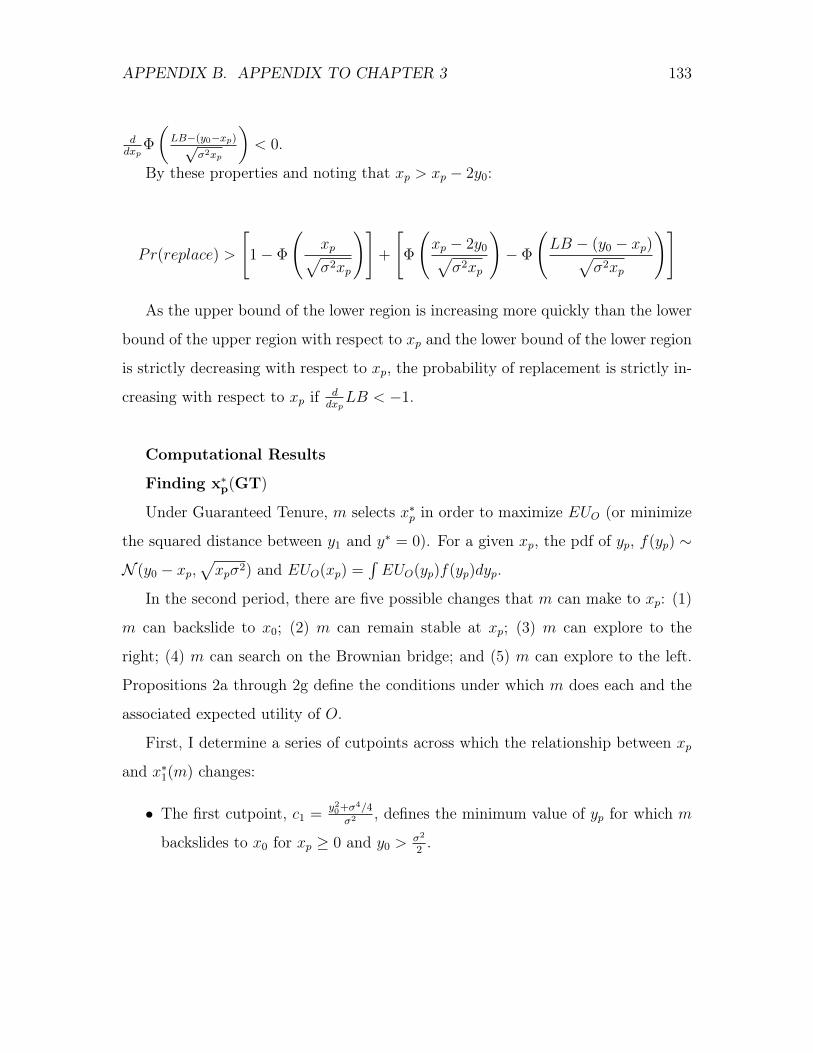
APPENDIX B. APPENDIX TO CHAPTER 3 133
ddx
p
�
✓LB�(y0�x
p
)p�2x
p
◆< 0.
By these properties and noting that xp > xp � 2y0:
Pr(replace) >
"1� �
xpp�2xp
!#+
"�
xp � 2y0p
�2xp
!� �
LB � (y0 � xp)p
�2xp
!#
As the upper bound of the lower region is increasing more quickly than the lower
bound of the upper region with respect to xp and the lower bound of the lower region
is strictly decreasing with respect to xp, the probability of replacement is strictly in-
creasing with respect to xp if ddx
p
LB < �1.
Computational Results
Finding x
⇤p(GT)
Under Guaranteed Tenure, m selects x⇤p in order to maximize EUO (or minimize
the squared distance between y1 and y⇤ = 0). For a given xp, the pdf of yp, f(yp) ⇠
N (y0 � xp,p
xp�2) and EUO(xp) =
REUO(yp)f(yp)dyp.
In the second period, there are five possible changes that m can make to xp: (1)
m can backslide to x0; (2) m can remain stable at xp; (3) m can explore to the
right; (4) m can search on the Brownian bridge; and (5) m can explore to the left.
Propositions 2a through 2g define the conditions under which m does each and the
associated expected utility of O.
First, I determine a series of cutpoints across which the relationship between xp
and x⇤1(m) changes:
• The first cutpoint, c1 =y20+�
4/4�2 , defines the minimum value of yp for which m
backslides to x0 for xp � 0 and y0 >�2
2 .

APPENDIX B. APPENDIX TO CHAPTER 3 134
• The second cutpoint, c2 = y0, defines the minimum value of yp for which m
backslides to x0 for y0 �2
2 .
• The third cutpoint, c3 =
q(y0 � �2
4 )�2, defines the minimum value of yp for
which m explores to the right from x0 for xp < 0 and y0 >�2
2 .
• The fourth cutpoint, c4 =
�2
2 , defines the minimum value of yp for which m
explores to the right from xp for xp � 0.
• The fifth cutpoint, c5 =
y0�p
y20+2xp
�2
2 , defines the minimum value of yp for
which m remains stable at xp for 0 xp 4y20�2 .
• The sixth cutpoint, c6 = �y0, defines the minimum value of yp for which m
remains stable at xp for xp >4y20�2 .
• The seventh cutpoint, c7 = y0� xp
�2
2y0, defines the minimum value of yp for which
m backslides to x0 for xp >4y20�2 .
Using these cutpoints, the following equation defines EUO(yp|xp) under r = GT :
• If xp < 0 and y0 >�2
2
EUO < � 1� �
xp + c3 � y0p
|xp|�2
!!✓y0 �
�2
4
◆�2�
Z c3
0
1p|xp|�2
�
xp + yp � y0p
|xp|�2
!y2pdyp

APPENDIX B. APPENDIX TO CHAPTER 3 135
• If xp < 0 and y0 �2
2
EUO < � 1� �
xp + c2 � y0p
|xp|�2
!!y20�
Z c2
0
1p|xp|�2
�
xp + yp � y0p
|xp|�2
!y2pdyp
• If 0 xp 4y20�2 and y0 >
�2
2
µ =
yp � y0xp
x⇤1(m) =
2µy0 + �2
2
⇣�2
xp
� µ2⌘
EUO = � 1� �
xp + c1 � y0p
|xp|�2
!!y20�
Z c1
c4
1p|xp|�2
�
xp + yp � y0p
|xp|�2
!✓yp �
�2
4
◆�2dyp�
Z c4
c5
1p|xp|�2
�
xp + yp � y0p
|xp|�2
!y2pdyp�
Z c5
�1
1p|xp|�2
�
xp + yp � y0p
|xp|�2
!✓(y0 + µx⇤
1(m))
2+
(xp � x⇤1(m))x⇤
1(m)
xp
�2
◆dyp

APPENDIX B. APPENDIX TO CHAPTER 3 136
• If 0 xp 4y20�2 and y0 <
�2
2
EUO = � 1� �
xp + c2 � y0p
|xp|�2
!!y20�
Z c2
c5
1p|xp|�2
�
xp + yp � y0p
|xp|�2
!y2pdyp�
Z c5
�1
1p|xp|�2
�
xp + yp � y0p
|xp|�2
!✓(y0 + µx⇤
1(m))
2+
(xp � x⇤1(m))x⇤
1(m)
xp
�2
◆dyp
• If xp >4y20�2 and y0 >
�2
2
EUO = � 1� �
xp + c1 � y0p
|xp|�2
!!y20�
Z c1
c4
1p|xp|�2
�
xp + yp � y0p
|xp|�2
!✓yp �
�2
4
◆�2dyp�
Z c4
c6
1p|xp|�2
�
xp + yp � y0p
|xp|�2
!y2pdyp�
�
xp + c6 � y0p
|xp|�2
!� �
xp + c7 � y0p
xp�2
!!y20�
Z c7
�1
1p|xp|�2
�
xp + yp � y0p
|xp|�2
!✓(y0 + µx⇤
1(m))
2+
(xp � x⇤1(m))x⇤
1(m)
xp
�2
◆dyp

APPENDIX B. APPENDIX TO CHAPTER 3 137
• If xp >4y20�2 and y0 �2
2
EUO = � 1� �
xp + c2 � y0p
|xp|�2
!!y20�
Z c2
c6
1p|xp|�2
�
xp + yp � y0p
|xp|�2
!✓yp �
�2
4
◆�2dyp�
�
xp + c6 � y0p
|xp|�2
!� �
xp + c7 � y0p
|xp|�2
!!y20�
Z c7
�1
1p|xp|�2
�
xp + yp � y0p
|xp|�2
!✓(y0 + µx⇤
1(m))
2+
(xp � x⇤1(m))x⇤
1(m)
xp
�2
◆dyp
The function “CompleteIntegral.GT” calculates EUO(yp|xp) under r = GT . It
utilizes a series of helper functions that calculate pieces of the partitioned density of
yp resulting from xp. The function “integrate_sg” corrects the output of the integral
for very high variance density functions:
integrand.1 = function(y_p, x_p = x_p, s2 = s2, y_0 = y_0) {
dnorm(y_p, y_0 - x_p, sqrt(abs(x_p) * s2)) * -(y_p - s2/4) *
s2
}
integrand.2 = function(y_p, x_p = x_p, s2 = s2, y_0 = y_0) {
EU_O <- -y_p^2
dnorm(y_p, y_0 - x_p, sqrt(abs(x_p) * s2)) * EU_O
}
integrand.3 = function(y_p, x_p = x_p, s2 = s2, y_0 = y_0) {
APPENDIX B. APPENDIX TO CHAPTER 3 138
mu_hat <- (y_p - y_0)/x_p
p2_star <- (2 * mu_hat * y_0 + s2)/(2 * (s2/x_p - mu_hat^2))
out <- -(y_0 + mu_hat * p2_star)^2 - ((x_p - p2_star) * p2_star *
s2)/x_p
dnorm(y_p, y_0 - x_p, sqrt(abs(x_p) * s2)) * out
}
CompleteIntegral.GT = function(x_p, s2, y_0) {
if (x_p > 0) {
c_1 <- (y_0^2 + s2^2/4)/s2
c_2 <- y_0
c_3 <- ifelse(y_0 >= s2/4, sqrt((y_0 - s2/4) * s2), NA)
c_4 <- s2/2
c_5 <- (y_0 - sqrt(y_0^2 + 2 * x_p * s2))/2
c_6 <- -y_0
c_7 <- y_0 - (x_p * s2)/(2 * y_0)
}
if (x_p < 0) {
c_1 <- (y_0^2 + s2/4)/s2
c_2 <- y_0
c_3 <- ifelse(y_0 >= s2/4, sqrt((y_0 - s2/4) * s2), NA)
}
APPENDIX B. APPENDIX TO CHAPTER 3 139
if (x_p == 0) {
return(-(y_0 - s2/4) * s2)
}
if (x_p < 0 & y_0 > s2/2) {
part1 <- -(1 - pnorm((x_p + c_3 - y_0)/sqrt(abs(x_p) *
s2))) * (y_0 - s2/4) * s2
part2 <- integrate(integrand.2, lower = 0, upper = c_3,
x_p = x_p, s2 = s2, y_0 = y_0)$value
return(part1 + part2)
}
if (x_p < 0 & y_0 <= s2/2) {
part1 <- -(1 - pnorm((x_p + c_2 - y_0)/sqrt(abs(x_p) *
s2))) * y_0^2
part2 <- integrate(integrand.2, lower = 0, upper = c_2,
x_p = x_p, s2 = s2, y_0 = y_0)$value
return(part1 + part2)
}
if (x_p > 0 & x_p <= 4 * y_0^2/s2 & y_0 > s2/2) {
part1 <- -(1 - pnorm((x_p + c_1 - y_0)/sqrt(abs(x_p) *
s2))) * y_0^2
part2 <- integrate_sg(integrand.1, lower = c_4, upper = c_1,
x_p = x_p, s2 = s2, y_0 = y_0)$value
APPENDIX B. APPENDIX TO CHAPTER 3 140
part3 <- integrate(integrand.2, lower = c_5, upper = c_4,
x_p = x_p, s2 = s2, y_0 = y_0)$value
part4 <- integrate(integrand.3, lower = -Inf, upper = c_5,
x_p = x_p, s2 = s2, y_0 = y_0)$value
return(part1 + part2 + part3 + part4)
}
if (x_p > 0 & x_p <= 4 * y_0^2/s2 & y_0 <= s2/2) {
part1 <- -(1 - pnorm((x_p + c_2 - y_0)/sqrt(abs(x_p) *
s2))) * y_0^2
part2 <- integrate_sg(integrand.2, lower = c_5, upper = c_2,
x_p = x_p, s2 = s2, y_0 = y_0)$value
part3 <- integrate_sg(integrand.3, lower = -Inf, upper = c_5,
x_p = x_p, s2 = s2, y_0 = y_0)$value
return(part1 + part2 + part3)
}
if (x_p > 4 * y_0^2/s2 & y_0 > s2/2) {
part1 <- -(1 - pnorm((x_p + c_1 - y_0)/sqrt(abs(x_p) *
s2))) * y_0^2
part2 <- integrate_sg(integrand.1, lower = c_4, upper = c_1,
x_p = x_p, s2 = s2, y_0 = y_0)$value
part3 <- integrate_sg(integrand.2, lower = c_6, upper = c_4,
x_p = x_p, s2 = s2, y_0 = y_0)$value
part4a <- pnorm((x_p + c_6 - y_0)/sqrt(abs(x_p) * s2)) -
APPENDIX B. APPENDIX TO CHAPTER 3 141
pnorm((x_p + c_7 - y_0)/sqrt(abs(x_p) * s2))
part4b <- -y_0^2
part5 <- integrate_sg(integrand.3, lower = -Inf, upper = c_7,
x_p = x_p, s2 = s2, y_0 = y_0)$value
return(part1 + part2 + part3 + part4a * part4b + part5)
}
if (x_p > 4 * y_0^2/s2 & y_0 <= s2/2) {
part1 <- -(1 - pnorm((x_p + c_2 - y_0)/sqrt(abs(x_p) *
s2))) * y_0^2
part2 <- integrate_sg(integrand.2, lower = c_6, upper = c_2,
x_p = x_p, s2 = s2, y_0 = y_0)$value
part3a <- pnorm((x_p + c_6 - y_0)/sqrt(abs(x_p) * s2)) -
pnorm((x_p + c_7 - y_0)/sqrt(abs(x_p) * s2))
part3b <- -y_0^2
part4 <- integrate_sg(integrand.3, lower = -Inf, upper = c_7,
x_p = x_p, s2 = s2, y_0 = y_0)$value
return(part1 + part2 + part3a * part3b + part4)
}
}
I now find xp that maximizes EUO(yp|xp) under GT. I maximize CompleteInte-
gral.GT using the function “optimise.GT”. The function uses a genetic optimization
routine to search for a global maximum.
APPENDIX B. APPENDIX TO CHAPTER 3 142
optimise.GT = function(s2, y_0) genoud(CompleteIntegral.GT, nvars = 1,
Domains = rbind(c(0.05, 4 * y_0)), boundary.enforcement = 0,
s2 = s2, y_0 = y_0, print.level = 0, max = T)
Finding x
⇤p(RS)
Under a Retrospective Satisficing replacement rule, m selects x⇤p in order to
maximize EUm(yp|xp), which is the probability that |yp| < y0. Pr(|yp| < y0) =
�
✓xpp
xp
�2
◆��
✓xp
�2y0pxp
�2
◆, which is calculated by the function “CompleteIntegral.RS”.
CompleteIntegral.RS = function(x_p, s2, y_0) {
-(pnorm(x_p/sqrt(abs(x_p) * s2)) - pnorm((x_p - 2 * y_0)/sqrt(abs(x_p) *
s2)))
}
I now find xp that maximizes EUm under RS. I maximize CompleteIntegral.GT
subject to the box constraint that 0 < xp y0 using Simulated Annuealing in the
function “optimise.RS”.
optimise.RS = function(s2, y_0) GenSA(y_0/2, CompleteIntegral.RS,
10^-8, y_0, control = list(verbose = FALSE, max.call = 1000),
s2 = s2, y_0 = y_0)
Finding yp⇤
Under a Outcome-based Replacement rule, O sets yp in order to maximize EUO.
Given yp, m then chooses x⇤p(OB) in order to minimize the probability of being
replaced. EUO(x⇤p(OB)|yp) under Outcome-based Replacement will be the calculated
in the same fashion as EUO(x⇤p(GT )) under Guaranteed Tenure, except that for
yp � y0 and yp yp, EUO = �⇣y0 � �2
4
⌘�2.

APPENDIX B. APPENDIX TO CHAPTER 3 143
The function “CompleteIntegral.OB” calculates EUO(yp) under r = OB:
EU_m.OB = function(x_p, LB, s2, y_0) {
UB <- y_0 - 10^(-5)
-((pnorm(UB, y_0 - x_p, sqrt(x_p * s2)) - pnorm(LB, y_0 -
x_p, sqrt(x_p * s2))))
}
x_p.star.OB = function(LB, s2, y_0) {
(optimise(EU_m.OB, lower = 10^-5, upper = y_0 - (LB + y_0)/2,
LB = LB, s2 = s2, y_0 = y_0, maximum = F)$minimum)
}
CompleteIntegral.OB = function(LB, s2, y_0) {
if (LB == -Inf)
return(-y_0^2)
if (LB >= y_0 - 2 * 10^-5) {
return(ifelse(y_0 <= s2/2, -y_0^2 - (LB - y_0 + 10^-5),
-(y_0 - s2/4) * s2 - (LB - y_0 + 10^-5)))
}
x_p <- x_p.star.OB(LB, s2, y_0)
c_1 <- y_0
c_4 <- s2/2
c_5 <- (y_0 - sqrt(y_0^2 + 2 * x_p * s2))/2
c_6 <- -y_0
c_7 <- y_0 - (x_p * s2)/(2 * y_0)

APPENDIX B. APPENDIX TO CHAPTER 3 144
if (y_0 > s2/2) {
top <- -(1 - pnorm((x_p + c_1 - y_0)/sqrt(abs(x_p) *
s2))) * (y_0 - s2/4) * s2
bottom <- -pnorm((x_p + LB - y_0)/sqrt(abs(x_p) * s2)) *
(y_0 - s2/4) * s2
} else {
top <- -(1 - pnorm((x_p + c_1 - y_0)/sqrt(abs(x_p) *
s2))) * y_0^2
bottom <- -pnorm((x_p + LB - y_0)/sqrt(abs(x_p) * s2)) *
y_0^2
}
if (x_p >= 0 & x_p <= 4 * y_0^2/s2 & y_0 > s2/2) {
if (LB > c_4) {
part1 <- integrate(integrand.1, lower = LB, upper = c_1,
x_p = x_p, s2 = s2, y_0 = y_0)$value
part2 <- part3 <- 0
} else if (LB > c_5) {
part1 <- integrate(integrand.1, lower = c_4, upper = c_1,
x_p = x_p, s2 = s2, y_0 = y_0)$value
part2 <- integrate(integrand.2, lower = LB, upper = c_4,
x_p = x_p, s2 = s2, y_0 = y_0)$value
part3 <- 0
} else {
part1 <- integrate(integrand.1, lower = c_4, upper = c_1,
x_p = x_p, s2 = s2, y_0 = y_0)$value
APPENDIX B. APPENDIX TO CHAPTER 3 145
part2 <- integrate(integrand.2, lower = c_5, upper = c_4,
x_p = x_p, s2 = s2, y_0 = y_0)$value
part3 <- integrate(integrand.3, lower = LB, upper = c_5,
x_p = x_p, s2 = s2, y_0 = y_0)$value
}
return(part1 + part2 + part3 + top + bottom)
} else if (x_p >= 0 & x_p <= 4 * y_0^2/s2 & y_0 <= s2/2) {
if (LB > c_5) {
part1 <- integrate(integrand.2, lower = LB, upper = c_1,
x_p = x_p, s2 = s2, y_0 = y_0)$value
part2 <- 0
} else {
part1 <- integrate(integrand.2, lower = c_5, upper = c_1,
x_p = x_p, s2 = s2, y_0 = y_0)$value
part2 <- integrate(integrand.3, lower = LB, upper = c_5,
x_p = x_p, s2 = s2, y_0 = y_0)$value
}
return(part1 + part2 + top + bottom)
} else if (x_p > 4 * y_0^2/s2 & y_0 > s2/2) {
if (LB > c_4) {
part1 <- integrate_sg(integrand.1, lower = LB, upper = c_1,
x_p = x_p, s2 = s2, y_0 = y_0)$value
part2 <- part3 <- part4 <- 0
} else if (LB > c_6) {
part1 <- integrate(integrand.1, lower = c_4, upper = c_1,
APPENDIX B. APPENDIX TO CHAPTER 3 146
x_p = x_p, s2 = s2, y_0 = y_0)$value
part2 <- integrate_sg(integrand.2, lower = LB, upper = c_4,
x_p = x_p, s2 = s2, y_0 = y_0)$value
part3 <- part4 <- 0
} else if (LB > c_7) {
part1 <- integrate(integrand.1, lower = c_4, upper = c_1,
x_p = x_p, s2 = s2, y_0 = y_0)$value
part2 <- integrate(integrand.2, lower = c_6, upper = c_4,
x_p = x_p, s2 = s2, y_0 = y_0)$value
part3 <- (pnorm((x_p + c_6 - y_0)/sqrt(abs(x_p) *
s2)) - pnorm((x_p + LB - y_0)/sqrt(abs(x_p) *
s2))) * -y_0^2
part4 <- 0
} else {
part1 <- integrate(integrand.1, lower = c_4, upper = c_1,
x_p = x_p, s2 = s2, y_0 = y_0)$value
part2 <- integrate(integrand.2, lower = c_6, upper = c_4,
x_p = x_p, s2 = s2, y_0 = y_0)$value
part3 <- (pnorm((x_p + c_6 - y_0)/sqrt(abs(x_p) *
s2)) - pnorm((x_p + c_7 - y_0)/sqrt(abs(x_p) *
s2))) * -y_0^2
part4 <- integrate_sg(integrand.3, lower = LB, upper = c_7,
x_p = x_p, s2 = s2, y_0 = y_0)$value
}
total <- part1 + part2 + part3 + part4 + top + bottom
APPENDIX B. APPENDIX TO CHAPTER 3 147
return(ifelse(round(total, 5) == -y_0^2, total + LB,
total))
} else if (x_p > 4 * y_0^2/s2 & y_0 <= s2/2) {
if (LB > c_6) {
part1 <- integrate(integrand.2, lower = LB, upper = c_1,
x_p = x_p, s2 = s2, y_0 = y_0)$value
part2 <- part3 <- 0
} else if (LB > c_7) {
part1 <- integrate(integrand.2, lower = c_6, upper = c_1,
x_p = x_p, s2 = s2, y_0 = y_0)$value
part2 <- (pnorm((x_p + c_6 - y_0)/sqrt(abs(x_p) *
s2)) - pnorm((x_p + LB - y_0)/sqrt(abs(x_p) *
s2))) * -y_0^2
part3 <- 0
} else {
part1 <- integrate_sg(integrand.2, lower = c_6, upper = c_1,
x_p = x_p, s2 = s2, y_0 = y_0)$value
part2 <- (pnorm((x_p + c_6 - y_0)/sqrt(abs(x_p) *
s2)) - pnorm((x_p + c_7 - y_0)/sqrt(abs(x_p) *
s2))) * -y_0^2
part3 <- integrate_sg(integrand.3, lower = LB, upper = c_7,
x_p = x_p, s2 = s2, y_0 = y_0)$value
}
total <- part1 + part2 + part3 + top + bottom
}

APPENDIX B. APPENDIX TO CHAPTER 3 148
}
I now find yp that maximizes EUO(yp) under OB. I maximize CompleteInte-
gral.OB using the function “optimise.OB”. The function uses a genetic optimization
routine to search for a global maximum.
optimise.OB = function(s2, y_0) genoud(CompleteIntegral.OB, nvars = 1,
Domains = rbind(c(-20 * y_0, y_0 - 10^-5)), boundary.enforcement = 0,
s2 = s2, y_0 = y_0, print.level = 0, max = T)

Bibliography
Adler, P. S. and Borys, B. (1996). Two Types of Bureaucracy: Enabling and Coercive.
Administrative Science Quarterly, 41(1):61–89.
Aghion, P. and Jackson, M. (2014). Inducing Leaders to Take Risky Decisions: Dis-
missal, Tenure, and Term Limits. National Bureau of Economic Research Working
Paper Series, No. 20301.
Agnone, J. (2007). Amplifying Public Opinion: The Policy Impact of the US Envi-
ronmental Movement. Social Forces, 85(4):1593–1620.
Allen, M., Raper, S., and Mitchell, J. (2001). Uncertainty in the IPCC’s Third
Assessment Report. Science, 293(5529):430–433.
Amenta, E., Caren, N., Chiarello, E., and Su, Y. (2010). The Political Consequences
of Social Movements. Annual Review of Sociology, 36(1):287–307.
Amenta, E., Carruthers, B. G., and Zylan, Y. (1992). A Hero for the Aged? The
Townsend Movement, the Political Mediation Model, and US Old-Age Policy,
1934-1950. American Journal of Sociology, 98(2):308–339.
Amenta, E., Dunleavy, K., and Bernstein, M. (1994). Stolen Thunder? Huey Long’s
149
BIBLIOGRAPHY 150
“Share Our Wealth,” Political Mediation, and the Second New Deal. American
Sociological Review, 59(5):678–702.
Anderson, P. and Tushman, M. L. (1990). Technological Discontinuities and Domi-
nant Designs: A Cyclical Model of Technological Change. Administrative Science
Quarterly, pages 604–633.
Andrews, K. T. and Edwards, B. (2004). Advocacy Organizations in the U.S. Political
Process. Annual Review of Sociology, 30(1):479–506.
Andrews, R. N. L. (2006). Managing the Environment, Managing Ourselves: A
History of American Environmental Policy. Yale University Press, New Haven,
2nd edition.
Austen-Smith, D. and Banks, J. S. (1999). Positive Political Theory I: Collective
Preference. Michigan Studies in Political Analysis. University of Michigan Press,
Ann Arbor.
Austen-Smith, D. and Banks, J. S. (2000). Cheap Talk and Burned Money. Journal
of Economic Theory, 91(1):1–16.
Barnard, C. I. (1938). The Functions of the Executive. Harvard University Press,
Cambridge.
Baron, J. N., Hannan, M. T., and Burton, M. D. (1999). Building the Iron Cage: De-
terminants of Managerial Intensity in the Early Years of Organizations. American
Sociological Review, 64(4):527–547.
Baumgartner, F. R. and Jones, B. D. (2009). Agendas and Instability in American
Politics. University of Chicago Press, Chicago, 2nd edition.
BIBLIOGRAPHY 151
Baumgartner, F. R. and Jones, B. D. (2015). The Politics of Information: Problem
Definition and the Course of Public Policy in America. The University of Chicago
Press, Chicago.
Baumgartner, F. R. and Leech, B. L. (1998). Basic Interests: The Importance of
Groups in Politics and in Political Science. Princeton University Press, Princeton,
N.J.
Bendor, J. (2010). Bounded Rationality and Politics. University of California Press,
Berkeley.
Bendor, J. and Meirowitz, A. (2004). Spatial Models of Delegation. American
Political Science Review, 98(2):293–310.
Bendor, J., Moe, T. M., and Shotts, K. W. (2001). Recycling the Garbage Can:
An Assessment of the Research Program. American Political Science Review,
95(1):169–190.
Bernstein, E. S. (2012). The Transparency Paradox a Role for Privacy in Orga-
nizational Learning and Operational Control. Administrative Science Quarterly,
57(2):181–216.
Berry, J. M. (1977). Lobbying for the People: The Political Behaviour of Public
Interest Groups. Princeton University Press, Princeton, N.J.
Beshears, J. and Gino, F. (2014). Experiment with Organizational Change Before
Going All In. HBR.org.
Black, D., Newing, R. A., McLean, I., McMillan, A., and Monroe, B. L. (1958). The
Theory of Committees and Elections. Cambridge University Press, New York.
BIBLIOGRAPHY 152
Blau, P. M. (1955). The Dynamics of Bureaucracy: A Study of Interpersonal Rela-
tions in Two Government Agencies. The University of Chicago Press, Chicago.
Bosso, C. J. (2005). Environment, Inc.: From Grassroots to Beltway. University
Press of Kansas, Lawrence.
Brocas, I. and Carillo, J. D. (2007). Influence Through Ignorance. RAND Journal
of Economics, 38(4):931–947.
Brown, P., Zavestoski, S., McCormick, S., Mayer, B., Morello-Frosch, R., and
Gasior Altman, R. (2004). Embodied Health Movements: New Approaches to
Social Movements in Health. Sociology of health & illness, 26(1):50–80.
Brudnick, I. A. (2011). The Congressional Research Service and the American Leg-
islative Process. Technical Report 7-5700, Congressional Research Service, Wash-
ington, D.C.
Burstein, P. (1998). Interest Organizations, Political Parties, and the Study of Demo-
cratic Politics. In Costain, A. N. and McFarland, A. S., editors, Social Movements
and American Political Institutions, pages 39–56. Rowman & Littlefield Publish-
ers, Oxford.
Burstein, P. and Freudenburg, W. (1978). Changing Public Policy: The Impact of
Public Opinion, Antiwar Demonstrations, and War Costs on Senate Voting on
Vietnam War Motions. American Journal of Sociology, 84(1):99–122.
Burstein, P. and Hirsh, C. E. (2007). Interest Organizations, Information, and Policy
Innovation in the U.S. Congress. Sociological Forum, 22(2):174–199.
Callander, S. (2008). A Theory of Policy Expertise. Quarterly Journal of Political
Science, 3(2):123–140.
BIBLIOGRAPHY 153
Callander, S. (2011a). Searching and Learning by Trial and Error. American Eco-
nomic Review, 101:2277–2308.
Callander, S. (2011b). Searching for Good Policies. American Political Science
Review, 105(4):643–662.
Callander, S. and Matouschek, N. (2014). Managing on Rugged Landscapes. Working
Paper.
Cameron, C. and McCarty, N. (2004). Models of Veto and Veto Bargaining. Annual
Reviews of Political Science, 7:409–435.
Canes-Wrone, B., Herron, M. C., and Shotts, K. W. (2001). Leadership and Pander-
ing: A Theory of Executive Policymaking. American Journal of Political Science,
45(3):532–550.
Cobb, M. D. and Kuklinski, J. H. (1997). Changing Minds: Political Arguments and
Political Persuasion. American Journal of Political Science, 41(1):88–121.
Cohen, K. J., Cyert, R. M., Dill, W. R., Kuehn, A. A., Miller, M. H., Van Wormer,
T. A., and Winters, P. R. (1960). The Carnegie Tech Management Game. The
Journal of Business, 33(4):303–321.
Cohen, M. D., March, J. G., and Olsen, J. P. (1972). A Garbage Can Model of
Organizational Choice. Administrative Science Quarterly, pages 1–25.
Cooper, J. (1970). The Origins of Standing Committees and the Development of the
Modern House. Rice University Studies, Houston.
Crawford, V. P. and Sobel, J. (1982). Strategic Information Transmission. Econo-
metrica: Journal of the Econometric Society, 50(6):1431–1451.
BIBLIOGRAPHY 154
Cress, D. M. and Snow, D. A. (2000). The Outcomes of Homeless Mobilization: The
Influence of Organization, Disruption, Political Mediation, and Framing. American
Journal of Sociology, 105(4):1063–1104.
Csaszar, F. A. (2013). An Efficient Frontier in Organization Design: Organizational
Structure as a Determinant of Exploration and Exploitation. Organization Science,
24(4):1083–1101.
Csaszar, F. A. and Eggers, J. P. (2013). Organizational Decision Making: An Infor-
mation Aggregation View. Management Science, 59(10):2257–2277.
Csaszar, F. A. and Levinthal, D. A. (2016). Mental Representation and the Discovery
of New Strategies. Strategic Management Journal.
Cyert, R. M. and March, J. G. (1963). A Behavioral Theory of the Firm. Blackwell,
Cambridge, 2nd edition.
Dalton, M. (1959). Men Who Manage: Fusions of Feeling and Theory in Adminis-
tration. John Wiley & Sons, New York.
Davis, J. P., Eisenhardt, K. M., and Bingham, C. B. (2007). Developing Theory
through Simulation Methods. Academy of Management Review, 32(2):480–499.
DeNardo, J. (1985). Power in Numbers. Princeton University Press, Princeton, N.J.
Denrell, J. (2003). Vicarious Learning, Undersampling of Failure, and the Myths of
Management. Organization Science, 14(3):227–243.
Denrell, J. and March, J. G. (2001). Adaptation as Information Restriction: The
Hot Stove Effect. Organization Science, 12(5):523–538.

BIBLIOGRAPHY 155
Diermeier, D. and Feddersen, T. J. (2000). Information and Congressional Hearings.
American Journal of Political Science, 44(1):51–65.
Diermeier, D. and Krehbiel, K. (2003). Institutionalism as a Methodology. Journal
of Theoretical Politics, 15(2):123–144.
DiMaggio, P. J. and Powell, W. W. (1983). The Iron Cage Revisited: Institutional
Isomorphism and Collective Rationality in Organizational Fields. American Soci-
ological Review, 48(2):147–160.
Downs, A. (1957). An Economic Theory of Political Action in a Democracy. Journal
of Political Economy, pages 135–150.
Edelman (2015). 2015 Edelman Trust Barometer Results. Technical report.
Eden, S. (1998). Environmental Issues: Knowledge, Uncertainty and the Environ-
ment. Progress in Human Geography, 22(3):425–432.
Eisenhardt, K. M. and Bourgeois, L. J. (1988). Politics of Strategic Decision Making
in High-Velocity Environments: Toward a Midrange Theory. Academy of Manage-
ment Journal, 31(4):737–770.
Epstein, S. (1996). Impure Science: AIDS, Activism, and the Politics of Knowledge.
Univ of California Press.
Erikson, R. S., MacKuen, M. B., and Stimson, J. A. (2002). The Macro Polity.
Cambridge University Press, New York.
Esterling, K. M. (2004). The Political Economy of Expertise. The University of
Michigan Press, Ann Arbor.
BIBLIOGRAPHY 156
Ethiraj, S. K. and Levinthal, D. (2009). Hoping for A to Z While Rewarding Only
A: Complex Organizations and Multiple Goals. Organization Science, 20(1):4–21.
Ezrahi, Y. (1990). The Descent of Icarus: Science and the Transformation of Con-
temporary Democracy. Harvard University Press, Cambridge.
Farber, D. A. (2003). Probabilities Behaving Badly: Complexity Theory and Envi-
ronmental Uncertainty. UC Davis L. Rev., 37:145.
Feldman, M. S. and March, J. G. (1981). Information in Organizations as Signal and
Symbol. Administrative Science Quarterly, 26(2):171–186.
Fleming, L. (2002). Finding the Organizational Sources of Technological Break-
throughs: The Story of Hewlett Packard’s Thermal Ink Jet. Industrial and Cor-
porate Change, 11(5):1059–1084.
Fleming, L. and Sorenson, O. (2004). Science as a Map in Technological Search.
Strategic Management Journal, 25:909–928.
Freeland, R. (2001). The Struggle for Control of the Modern Corporation: Organi-
zational Change at General Motors, 1924-1970. Cambridge University Press, New
York.
Fudenberg, D. and Tirole, J. (1991). Game Theory. MIT Press, Cambridge.
Gavetti, G., Greve, H. R., Levinthal, D. A., and Ocasio, W. (2012). The Behavioral
Theory of the Firm: Assessment and Prospects. Academy of Managament Annals,
6(1):1–40.
Gavetti, G. and Levinthal, D. (2000). Looking Forward and Looking Backward:
BIBLIOGRAPHY 157
Cognitive and Experiential Search. Administrative Science Quarterly, 45(1):113–
137.
Gavetti, G., Levinthal, D., and Ocasio, W. (2007). Perspective–Neo-Carnegie: The
Carnegie School’s Past, Present, and Reconstructing for the Future. Organization
Science, 18(3):523–536.
Gertner, J. (2012). The Idea Factory: Bell Labs and the Great Age of American
Innovation. The Penguin Press, New York.
Gibbons, R. (2003). Team Theory, Garbage Cans, and Real Organizations: Some
History and Prospects of Economic Research on Decision-Making in Organizations.
Industrial and Corporate Change, 12(4):753–787.
Gibbons, R., Matouschek, N., and Roberts, J. (2012). Decisions in Organizations. In
Gibbons, R. and Roberts, J., editors, The Handbook of Organizational Economics,
pages 373–431. Princeton University Press, Princeton.
Gibbons, R. and Roberts, J. (2012). Economic Theories of Incentives in Organiza-
tions. In Gibbons, R. and Roberts, J., editors, The Handbook of Organizational
Economics, pages 56–99. Princeton University Press, Princeton.
Gilligan, T. W. and Krehbiel, K. (1987). Collective Decisionmaking and Standing
Committees: An Informational Rationale for Restrictive Amendment Procedures.
Journal of Law, Economics, & Organization, 3(2):287–335.
Gilligan, T. W. and Krehbiel, K. (1989). Asymmetric Information and Legislative
Rules with a Heterogeneous Committee. American Journal of Political Science,
33(2):459–490.
BIBLIOGRAPHY 158
Gilligan, T. W. and Krehbiel, K. (1990). Organization of Informative Committees
by a Rational Legislature. American Journal of Political Science, 34(2):531–564.
Gillion, D. Q. (2012). Protest and Congressional Behavior: Assessing Racial and
Ethnic Minority Protests in the District. Journal of Politics, 74(04):950–962.
Gillion, D. Q. (2013). The Political Power of Protest: Minority Activism and Shifts
in Public Policy. Cambridge University Press, New York.
Giugni, M. (2004). Social Protest and Policy Change: Ecology, Antinuclear, and
Peace Movements in Comparative Perspective. Rowman & Littlefield, New York.
Granovetter, M. (2005). The Impact of Social Structure on Economic Outcomes.
Journal of Economic Perspectives, 19(1):33–50.
Granovetter, M. and Swedberg, R. (2011). The Sociology of Economic Life. Westview
Press, Boulder, third edition.
Habermas, J. (1971). Toward a Rational Society: Student Protest, Science, and
Politics, volume 404. Beacon Press.
Hadden, J. (2015). Networks in Contention. Cambridge University Press, New York.
Hall, R. L. and Deardorff, A. V. (2006). Lobbying as Legislative Subsidy. American
Political Science Review, 100(1):69–84.
Hamel, G. and Spence, S. (2010). Innovation Democracy: W.L. Gore’s Original
Management Model. Management Innovation Exchange.
Hannan, M. T. and Freeman, J. (1984). Structural Inertia and Organizational
Change. American Sociological Review, 49(2):149–164.
BIBLIOGRAPHY 159
Hansen, J. M. (1991). Gaining Access: Congress and the Farm Lobby, 1919-1981.
University of Chicago Press, Chicago.
Harrison, J. R., Lin, Z., Carroll, G. R., and Carley, K. M. (2007). Simulation
Modeling in Organizational and Management Research. Academy of Management
Review, 32(4):1229–1245.
Heinz, J. P., Laumann, E., Nelson, R., and Salisbury, R. (1993). The Hollow Core:
Private Interests in National Policy Making. Harvard University Press, Cambridge.
Holmstrom, B. and Ricart i Costa, J. (1986). Managerial Incentives and Capital
Management. Quarterly Journal of Economics, 101(4):835–860.
Ingram, P. and Simons, T. (2000). State Formation, Ideological Competition, and
the Ecology of Israeli Workers’ Cooperatives, 1920-1992. Administrative Science
Quarterly, 45(1):25–53.
Jamison, A. (2001). The Making of Green Knowledge: Environmental Politics and
Cultural Transformation. Cambridge University Press, New York.
Jenkins, J. C. (1987). Non-Profit Organizations and Policy Advocacy. In Powell, W.,
editor, Non-Profit Organization: A Handbook. Yale University Press, New Haven.
Johnson, E. W., Agnone, J., and McCarthy, J. D. (2010). Movement Organizations,
Synergistic Tactics and Environmental Public Policy. Social Forces, 88(5):2267–
2292.
Johnson, S. (2006). The Ghost Map: The Story of London’s Most Terrifying
Epidemic–and How It Changed Science, Cities, and the Modern World. River-
head Books, New York.
BIBLIOGRAPHY 160
Kaiser, R. (2013). Act of Congress: How America’s Essential Institution Works, and
How It Doesn’t. Alfred A. Knopf, New York.
Kamenica, E. and Gentzkow, M. (2011). Bayesian Persuasion. American Economic
Review, 101(6):2590–2615.
Kane, M. (2003). Social Movement Policy Success: Decriminalizing State Sodomy
Laws, 1969–1998. Mobilization: An International Quarterly, 8(3):313–334.
Kauffman, S. A. (1993). The Origins of Order: Self Organization and Selection in
Evolution. Oxford University Press, New York.
Kelley, T. and Littman, J. (2001). The Art of Innovation: Lessons in Creativity from
IDEO, America’s Leading Design Firm. Currency/Doubleday, New York.
King, B. G., Bentele, K. G., and Soule, S. A. (2007). Protest and Policymaking:
Explaining Fluctuation in Congressional Attention to Rights Issues, 1960–1986.
Social Forces, 86(1):137–163.
King, B. G., Cornwall, M., and Dahlin, E. C. (2005). Winning Woman Suffrage One
Step at a Time: Social Movements and the Logic of the Legislative Process. Social
Forces, 83(3):1211–1234.
King, D. C. (1994). The Nature of Congressional Committee Jurisdictions. American
Political Science Review, 88(1):48–62.
King, D. C. (1997). Turf Wars: How Congressional Committees Claim Jurisdiction.
University of Chicago Press, Chicago.
Kingdon, J. W. (1984). Agendas, Alternatives, and Public Policies. Little, Brown,
Boston.
BIBLIOGRAPHY 161
Knudsen, T. and Levinthal, D. A. (2007). Two Faces of Search: Alternative Gener-
ation and Alternative Evaluation. Organization Science, 18(1):39–54.
Koempel, M. L. and Schneider, J. (2007). Congressional Deskbook: The Practical
and Comprehensive Guide to Congress. TheCapitol.Net.
Kogut, B. and Zander, U. (1992). Knowledge of the Firm, Combinative Capabilities,
and the Replication of Technology. Organization Science, 3(3):383–397.
Kollman, K. (1998). Outside Lobbying: Public Opinion and Interest Group Strategies.
Princeton University Press, Princeton.
Kosar, K. R. (2015). Why I Quit the Congressional Research Service. Washington
Monthly.
Krehbiel, K. (1988). Spatial Models of Legislative Choice. Legislative Studies Quar-
terly, 13(3):259–319.
Krehbiel, K. (1991). Information and Legislative Organization. University of Michi-
gan Press, Ann Arbor.
Krehbiel, K. (1997). Pivotal Politics: A Theory of U.S. Lawmaking. University of
Chicago Press, Chicago.
Krehbiel, K. (2004). Legislative Organization. Journal of Economic Perspectives,
18(1):113–128.
Lashinsky, A. (2006). Chaos By Design. Fortune.
Levinthal, D. A. (1997). Adaptation on Rugged Landscapes. Management Science,
43(7):934–950.

BIBLIOGRAPHY 162
Levinthal, D. A. and March, J. G. (1993). The Myopia of Learning. Strategic
Management Journal, 14:95–112.
Levitt, B. and March, J. G. (1988). Organizational Learning. Annual Reviews of
Sociology, 14:319–40.
Leyden, K. M. (1995). Interest Group Resources and Testimony at Congressional
Hearings. Legislative Studies Quarterly, 20(3):431–439.
Lindbergh, B. and Miller, S. (2016). The Only Rule Is It Has To Work. Henry Holt
and Co., New York. Apple E-book.
Lippman, S. A. and McCall, J. J. (1976). The Economics of Job Search: A Survey.
Economic Inquiry, 14(2):155–189.
Lipsky, M. (1968). Protest as a Political Resource. American Political Science
Review, 62(04):1144–1158.
Lohmann, S. (1993). A Signaling Model of Informative and Manipulative Political
Action. American Political Science Review, 87(02):319–333.
Lyon, T. P. and Maxwell, J. W. (2008). Corporate Social Responsibility and the
Environment: A Theoretical Perspective. Review of Environmental Economics
and Policy, 2(2):240–260.
March, J. G. (1962). The Business Firm as a Political Coalition. Journal of Politics,
24(4):662–678.
March, J. G. (1991). Exploration and Exploitation in Organizational Learning. Or-
ganization Science, 2(1):71–87.
BIBLIOGRAPHY 163
March, J. G. (2006). Rationality, Foolishness, and Adaptive Intelligence. Strategic
Management Journal, 27(3):201–214.
March, J. G. (2010). The Ambiguities of Experience. Cornell University Press, Ithaca.
March, J. G. and Shapira, Z. (1987). Managerial Perspectives on Risk and Risk
Taking. Management Science, 33(11):1404–1418.
March, J. G. and Simon, H. A. (1958). Organizations. Wiley, New York.
Matthews, S. A. (1989). Veto Threats: Rhetoric in a Bargaining Game. Quarterly
Journal of Economics, 104(2):347–369.
McAdam, D. and Su, Y. (2002). The War at Home: Antiwar Protests and Congres-
sional Voting, 1965 to 1973. American Sociological Review, pages 696–721.
McCammon, H. J., Campbell, K. E., Granberg, E. M., and Mowery, C. (2001). How
Movements Win: Gendered Opportunity Structures and U.S. Women’s Suffrage
Movements, 1866 to 1919. American Sociological Review, 66(1):49–70.
Mebane Jr., W. R. and Sekhon, J. S. (2011). Genetic Optimization Using Derivatives:
The Rgenoud Package for R. Journal of Statistical Software, 42(11):1–26.
Milgrom, P. and Roberts, J. (1988). An Economic Approach to Influence Activities
in Organizations. American Journal of Sociology, 94(Supplement: Organizations
and Institutions: Sociological and Economic Approaches to the Analysis of Social
Structure):S154–S179.
Mitchell, G. J. (2007). Report to the Commission of Baseball of an Independent
Investigation into the Illegal Use of Steroids and Other Performance Enhancing
BIBLIOGRAPHY 164
Substances by Players in Major League Baseball. Technical report, DLA Piper US
LLP.
Moe, T. M. (2012). Delegation, Control, and the Study of Public Bureaucracy. In
The Forum, volume 10.
Morales, D. M. (2013). Policymaking as Gift Exchange: An Ethnographic Study of
Lobbyists. Dissertation, Stanford University, Stanford, CA.
Morrill, C. (1991). Conflict Management and Organizational Change. American
Journal of Sociology, 97(3):585–621.
Morrill, C. (1995). The Executive Way: Conflict Management in Organizations.
University of Chicago Press, Chicago.
Mullen, K. M. (2014). Continuous Global Optimization in R. Journal of Statistical
Software, 60(6):1–45.
Nelkin, D. (1975). The Political Impact of Technical Expertise. Social Studies of
Science, 5(1):35–54.
Nelson, R. R. and Winter, S. G. (1982). An Evolutionary Theory of Economic
Change. The Belknap Press of Harvard University Press, Cambridge.
Oleszek, W. J. (1989). Congressional Procedures and the Policy Process. Congres-
sional Quarterly Press, Washington, 3rd edition.
Olzak, S. and Soule, S. A. (2009). Cross-Cutting Influences of Environmental Protest
and Legislation. Social Forces, 88(1):201–225.
O’Reilly, C. A. and Tushman, M. L. (2013). Organizational Ambidexterity: Past,
Present, and Future. Academy of Management Perspectives, 27(4):324–338.
BIBLIOGRAPHY 165
Page, B. I. and Shapiro, R. Y. (1983). Effects of Public Opinion on Policy. American
Political Science Review, 77(1):175–190.
Pfeffer, J. (1981). Power in Organizations. Ballinger Pub. Co., Cambridge.
Pfeffer, J. and Sutton, R. I. (2006a). Evidence-based Management. Harvard Business
Review.
Pfeffer, J. and Sutton, R. I. (2006b). Hard Facts, Dangerous Half-Truths, and Total
Nonsense. Harvard Business School Press, Boston.
Pondy, L. R. (1992). Reflections on Organizational Conflict. Journal of Organiza-
tional Behavior, 13:257–261.
Rao, H., Morrill, C., and Zald, M. N. (2000). Power Plays: How Social Movements
and Collective Action Create New Organizational Forms. Research in Organiza-
tional Behavior, 22:239–82.
Rivkin, J. W. (2000). Imitation of Complex Strategies. Management Science,
46(6):824–844.
Rivkin, J. W. and Siggelkow, N. (2003). Balancing Search and Stability: Inter-
dependencies Among Elements of Organizational Design. Management Science,
49(3):290–311.
Roberts, J., Saloner, G., and Gibbons, R. (2012). Strategy in Organizations. In
Gibbons, R. and Roberts, J., editors, The Handbook of Organizational Economics,
pages 373–431. Princeton University Press, Princeton.
Rome, A. (2013). The Genius of Earth Day: How a 1970 Teach-in Unexpectedly
Made the First Green Generation. Hill and Wang, New York.
BIBLIOGRAPHY 166
Sabatier, P. A. (1991). Toward Better Theories of the Policy Process. PS: Political
Science & Politics, 24(2):147–156.
Sachs, R. C. (2003). A Guide to Congressional Hearings. Novinka Books, New York.
Sah, R. K. and Stiglitz, J. E. (1986). The Architecture of Economic Systems: Hier-
archies and Polyarchies. American Economic Review, 76(4):716–727.
Santoro, W. A. (2002). The Civil Rights Movement’s Struggle for Fair Employment:
A “Dramatic Events–Conventional Politics” Model. Social Forces, 81(1):177–206.
Santoro, W. A. (2008). The Civil Rights Movement and the Right to Vote: Black
Protest, Segregationist Violence and the Audience. Social Forces, 86(4):1391–1414.
Schilling, M. A. and Fang, C. (2014). When Hubs Forget, Lie, and Play Favorites: In-
terpersonal Network Structure, Information Distortion, and Organizational Learn-
ing. Strategic Management Journal, 35(7):974–994.
Schlozman, K. L. and Tierney, J. T. (1986). Organized Interests and American
Democracy. Harper and Row, New York.
Scott, W. R. (1987). Organizations. Prentice Hall, Englewood Cliffs, NJ.
Shaiko, R. G. (1999). Voices and Echoes for the Environment: Public Interest Rep-
resentation in the 1990s and Beyond. Columbia University Press, New York.
Shapira, Z. (1995). Risk Taking: A Managerial Perspective. Russell Sage Foundation.
Shepsle, K. A. (1992). Congress Is a “They,” Not an “It”: Legislative Intent as
Oxymoron. International Review of Law and Economics, 12(2):239–256.
BIBLIOGRAPHY 167
Shepsle, K. A. and Weingast, B. R. (1981). Structure Induced Equilibrium and
Legislative Choice. Public Choice, 37:503–519.
Shepsle, K. A. and Weingast, B. R. (1987). The Institutional Foundations of Com-
mittee Power. American Political Science Review, 81(1):85–104.
Simon, H. A. (1955). A Behavioral Model of Rational Choice. Quarterly Journal of
Economics, 69(1):99–118.
Simon, H. A. (1976). Administrative Behavior: A Study of Decision-making Processes
in Administrative Organization. Free Press, New York, 3rd edition edition.
Smith, S. S. and Deering, C. J. (1997). Committees in Congress. CQ Press, Wash-
ington, D.C., 3rd edition.
Soule, S. and King, B. (2006). The Stages of the Policy Process and the Equal Rights
Amendment, 1972–1982. American Journal of Sociology, 111(6):1871–1909.
Soule, S., McAdam, D., McCarthy, J., and Su, Y. (1999). Protest Events: Cause
or Consequence of State Action? The U.S. Women’s Movement and Federal Con-
gressional Activities, 1956–1979. Mobilization, 4(2):239.
Soule, S. A. (2004). Going to the Chapel? Same-sex Marriage Bans in the United
States, 1973-2000. Social Problems, 51(4):453–477.
Soule, S. A. (2009). Contention and Corporate Social Responsibility. Cambridge
University Press, New York.
Soule, S. A. (2012). Social Movements and Markets, Industries, and Firms. Organi-
zation Studies, 33(12):1715–1733.
BIBLIOGRAPHY 168
Soule, S. A. and Olzak, S. (2004). When Do Movements Matter? The Politics of
Contingency and the Equal Rights Amendment. American Sociological Review,
69(4):473–497.
Stone, C. D. (1993). The Gnat Is Older Than Man: Global Environment and Human
Agenda. Princeton University Press, Princeton, N.J.
Sutton, R. I. and Hoyt, D. (2016). Better Service, Faster: A Design Thinking Case
Study. Harvard Business Review.
Talbert, J. C., Jones, B. D., and Baumgartner, F. R. (1995). Nonlegislative Hearings
and Policy Change in Congress. American Journal of Political Science, 39(2):383–
405.
Thompson, J. D. (1967). Organizations in Action: Social Science Bases of Admin-
istrative Theory. Transaction Publishers, New Brunswick.
Tushman, M. L. and Anderson, P. (1986). Technological Discontinuities and Orga-
nizational Environments. Administrative Science Quarterly, 31(3):439–465.
Tushman, M. L. and O’Reilly, C. A. (1996). The Ambidextrous Organizations: Man-
aging Evolutionary and Revolutionary Change. California Management Review,
38(4):8–30.
Utterback, J. (1994). Mastering the Dynamics of Innovation: How Companies Can
Seize Opportunities in the Face of Technological Change. Harvard Business School
Press, Boston.
Vancil, R. F. (1979). Decentralization: Managerial Ambiguity by Design. Dow Jones-
Irwin, Homewood, Ill.
BIBLIOGRAPHY 169
Walker, J. L. (1991). Mobilizing Interest Groups in America: Patrons, Professions,
and Social Movements. University of Michigan Press, Ann Arbor.
Weber, K., Rao, H., and Thomas, L. G. (2009). From Streets to Suites: How the Anti-
Biotech Movement Affected German Pharmaceutical Firms. American Sociological
Review, 74(1):106–127.
Weber, M. (1978). Economy and Society: An Outline of Interpretive Sociology.
University of California Press, Berkeley.
Weiss, C. H. (1992). Helping Government Think: Functions and Consequences of
Policy Analysis Organizations. In Organizations for Policy Analysis. Sage Publi-
cations, Newbury Park, CA.
Wilson, J. Q. (1973). Political Organizations. New York, Basic Books,.
Wright, J. R. (1995). Interest Groups and Congress: Lobbying, Contributions, and
Influence. Allyn & Bacon, Boston.
Xiang, Y., Gubian, S., Suomela, B., and Hoeng, J. (2013). Generalized Simulated
Annealing for Global Optimization: The GenSA Package. R Journal, 5(1):13–28.
Zald, M. N. (1970). Organizational Change: The Political Economy of the YMCA.
University of Chicago Press, Chicago.
Zbaracki, M. J. and Bergen, M. (2010). When Truces Collapse: A Longitudinal
Study of Price-adjustment Routines. Organization Science, 21(5):955–972.