thermoelectric phenomena introductionph5060/manuals/seebeck.pdfthermoelectric phenomena introduction...
TRANSCRIPT

Thermoelectric Phenomena Introduction
The Peltier effect was first observed in 1834 by the Frenchman Jean C.A. Peltier. It describes the heat
current that arises as a result of an electric current through the interface of two different conductors.
The purpose of this project is to measure the maximum cooling of a commercial Peltier element, in
terms of the lowest achievable temperature inside a small refrigerator built using the element. The
project also includes investigating the limiting factors of Peltier cooling and presenting the relevant
theory behind it.
Theory
The heat current, ABQ , at an interface between two conductors (A and B) can be expressed as a function
of the electrical current, I, through the interface, and the Peltier coefficients of the two materials, ΠA
and ΠB. The heat current at the interface is:
IQ BAAB )( (1)
Heat is generated if ΠA> ΠB and the electrical current flows from A to B. If the direction of the
electrical current is reversed, so is the direction of the heat current.
By combining two interfaces, A to B and B to A, a hot and a cold junction can be created. In this case,
heat is generated at one of the interfaces and the same amount is absorbed at the other.
In most commercial Peltier elements, three different materials are used (a P-doped semiconductor (P),
a metal (M) and an N-doped semiconductor (N)). The Peltier coefficients of the three materials are
different, ΠN> ΠM> ΠP. If the materials are arranged according to figure 1, a hot and a cold side are
created, using several interfaces between the materials (and thus maximizing the cooling) with simple
serial electrical connections. The arrangement functions due to the fact that (for the materials given in
this example) heat is generated at junctions of the type M to P and N to M and absorbed at junctions M
to N and P to M.
Figure 1: Sketch of a commercial Peltier element.
The cooling ability of a Peltier element is limited by several factors. Even though the Peltier cooling
increases linearly with the electric current through the element, an increased current does not always

lead to increased cooling. As the electric current increases, so does the resistive heating of the entire
element. At some point, the resistive heating caused by an increasing electric current will be larger
than the cooling caused by the Peltier effect.
At a constant current the temperature difference between the hot and the cold side, ∆T, will be
constant. This gives rise to another limiting factor, namely the heat dissipation on the hot side. If the
heat generated on the hot side is not dissipated into the environment, the temperature of the hot side
will be increased. Since the temperature difference between the sides is constant, this leads to an equal
increase in the temperature of the cold side. The heat conduction through the element depends linearly
on the temperature difference between the sides. Since the temperature difference increases with the
electric current through the element, so does the conduction of heat through the element.
For each pair of hot/cold interfaces (eg. metal-semiconductor-metal), the cooling, P, (eg. the flow of
thermal energy from the cold to the hot side) is related to the Peltier coefficients of the two materials,
ΠA and ΠB (where it is assumed that ΠA>ΠB), the electric resistance of the element, R, the electric
current, I, the thermal conductivity of the element, K, and the temperature difference between the sides
of the element, ΔT, according to equation 2.
TKIR
IP BA
2
)(2
(2)
In this case, since cooling is the parameter of interest, the heat flow is described in this slightly unusual
way (strictly speaking as flow of “cold”, or negative flow of heat).
As seen from equation 2, the Peltier cooling (the first term) depends linearly on the electric current,
whereas the resistive heating (the second term) is related to the square of the electrical current. The
third term describes the conduction of heat through the Peltier element and relates to the temperature
difference between the hot and cold sides, ΔT. The relationship between ΔT and the electrical current is
unknown. At low electric currents, the Peltier cooling is the dominating term, but as the electric current
increases, the resistive heating will increase faster than the Peltier cooling. At a certain value of the
electric current, the resistive heating will be larger than the Peltier cooling, and any further increase in
electric current will actually decrease the cooling.
By setting the derivative of the cooling P in equation 2 with respect to the current I to zero the current
at maximum cooling can be obtained.
0
I
TKIR
I
PBA (3)
From equation 3, the current at maximum cooling, I0, can be determined.
R
I
TK
IBA )(
0
(4)
In equations 3 and 4, the unknown dependence of ΔT on the current, I, is included. This must be
measured experimentally or estimated in order to calculate an optimum current from equation 4.
It should be noted that the above stated equations are valid for a single pair of material interfaces. For a
commercial Peltier element, the contribution from all interfaces must be added in order to obtain total
values of cooling power, current at optimum cooling etc. This requires knowledge of the number of
interfaces in the element, as well as the Peltier coefficients of all participating materials.
For an element consisting of nMP pairs of interfaces between metal and p-doped semiconductor, and
nMN pairs of interfaces between metal and n-doped semiconductor, the total cooling power would be
described by equation 5 (obtained by modification of equation 2). For a symmetrically built Peltier
element, it is of course true that nMP=nMN.
TKIR
InInP MNMNPMMPtotal
2
2
(5)
In equation 5, the Peltier element is considered as a single unit regarding the heat conduction and
resistive heating. The resistance, R, in the equation describes the total electrical resistance of the Peltier
element. It is worth noting that the current is the same through each of the interfaces as through the
entire element (since they are connected in series). For practical purposes, it would also be possible to
assign a total Peltier coefficient to the entire element, thus incorrectly regarding it as a single pair of
material interfaces. In this case, equation 2 can be used, with the total Peltier coefficient replacing the
term (ΠA-ΠB):
TKIR
IP totaltotal
2
2
(6)
Adapted from `Testing a Peltier Element’
home.student.uu.se/hany4287/Peltier%20element.doc
Several experiments can be performed with a peltier element or thermoelectric coolers (TEC)
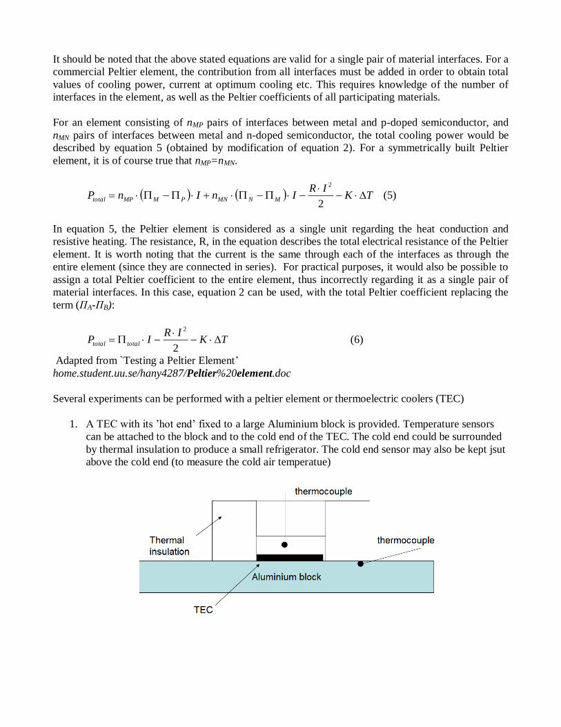
1. A TEC with its ’hot end’ fixed to a large Aluminium block is provided. Temperature sensors
can be attached to the block and to the cold end of the TEC. The cold end could be surrounded
by thermal insulation to produce a small refrigerator. The cold end sensor may also be kept jsut
above the cold end (to measure the cold air temperatue)

2. Determine the maximum current and voltage the TEC can tolerate. Obvioulsy you should
operate well below these limits
3. Measure the voltage across the TEC, ,the temperature inside the cavity and the temperature of
the Al block as a function of the current through the TEC. Plot the cavity temperature and the
temperature difference as a function of the current and analyze the plot.
The thermal conductivity of the entire refrigerator and the total Peltier coefficient of the element can be
roughly estimated using equation 6 and the polynomial fitted to the curve in figure 6, together with the
assumptions that the thermal flow through the refrigerator walls are linearly dependent on the
temperature difference between the cavity and the surroundings, ΔT. It is also assumed the thermal
conductivity of the Peltier element and the refrigerator walls do not vary with temperature.
For a stationary temperature, the cooling power of the Peltier element (from equation 6) is equal to the
thermal flow through the refrigerator walls (including both conducted and radiated heat). If this flow is
assumed to depend linearly on ΔT through some constant C, equation 6 can be written as:
TKRI
ITCP totaltotal 2
2
(7)
This implies that ΔT can be written as a second order function on the current, I, through the element.
2
2)(I
KC
RI
KCT total
(8)
Determine the Peltier coefficient Πtotal. What information can you get from this number?
What are the factors that affect the measurement? What can you do to make this a better refrigerator?
4. A second TEC can be fixed to the Al block with screws, temperature sensors and a heating
element as shown below:
(you could use thermistors or thermocouples)
figure courtesy: Experiments and Demonstrations in Physics, Yaakov Kraftmakher, Bar-Ilan
Physics Laboratory, World Scientific

5. Apply a signal from a function gerenator with the hot-end on top first and then with the cold-
end on top. Measure the temperature at both ends and plot as a fucntion of time. At the end of
2-3 minutes you could increase the amplitude of the signal and measure for the next 2-3
minutes. Repeat for a few amplitudes. Plot T (temp. difference) as a function of time. Explain
your observations.
6. Repeat the above process now with DC current.
7. Determine the Seebeck coefficient of the TEC by measuring the voltage across the TEC and
T by heating the top side of the TEC using the heater (dont connect a power supply to the
TEC). Repeat this measurement by placing the bottom-side on top.
8. How can you determine the thermal conductivity of the TEC?
9. Review the following writeup (atleast upto fig. 8!) from: Experiments and
Demonstrations in Physics, Yaakov Kraftmakher, Bar-Ilan Physics Laboratory, World
Scientific
10. Attempt to reproduce the experimental tasks and analysis outlined. INFORM THE
INSTRUCTOR IF YOU HAVE SPECIFIC DIFFICULTY IN DOING THIS.


Further Information


PE-127-10-13


Thermoelectric Cooler
1. Demonstration of the Peltier effect and calibration of the thermocouple
2. Insulate thermocouple, keep thermocouple in slab and on top of TEC. Measure,
V, T1, T2, by changing the current through the TEC. Give time for stabilization
after each current. Plot cold-end temperature and temperature difference vs.
current.
3. Repeat the measurement with the thermocouple above the cold-end of the TEC
(in the insulated air-gap).
4. Use both data sets to determine the Peltier coefficient. Can you find the thermal
conductivity of the element? What information can you get from this number?
What information can you get from this number? What are the factors that affect
the measurement? What can you do to make this a better refrigerator?
5. Place the TEC mounted on the circular slab on an ice bath. Apply some heat to
the top end of the TEC with a heater. Measure V, T1, T2 as a function of the heat
supplied. Plot V vs. temp-difference to determine the Seebeck coefficient. Repeat
the experiment with the bigger Aluminium slab and compare your results.
6. Place the TEC mounted (cooling side up) on the circular slab on the large Al block.
Vary the current through the TEC. For each current, apply power to the heater
such that the temperature difference between the sides is nearly zero.
Determine the Peltier coefficient. What is the difference between this method
and that described above?
7. Think of a way to determine the coefficient of performance of the TEC as a
function of current.
8. Place TEC mounted on the circular slab on an ice bath with the cooling side on
top. Apply power to the heater such that the top side is nearly at room
temperature. Monitor the voltage across the module. Use the data to determine
the figure of merit of TEC. Read the manual carefully before doing this. DO NOT
EXCEED A TEMPERATURE OF 60 dec C