thermal performance of fire resistive materials

NISTIR 7401

Thermal Performance of Fire Resistive Materials I. Characterization with Respect to Thermal Performance Models

Dale P. Bentz Kuldeep R. Prasad

NISTIR 7401

Thermal Performance of Fire Resistive Materials I. Characterization with Respect to Thermal Performance Models

Dale P. Bentz Kuldeep R. Prasad

Building and Fire Research Laboratory National Institute of Standards and Technology

Gaithersburg, MD 20899-8615

February 2007

U.S. DEPARTMENT OF COMMERCE Carlos M. Gutierrez, Secretary

TECHNOLOGY ADMINISTRATION Michele O’Neill, Acting Under Secretary of Commerce for Technology

NATIONAL INSTITUTE OF STANDARDS AND TECHNOLOGY William Jeffrey, Director

ii

Abstract Fire resistive materials (FRMs) are currently qualified and certified based on lab-scale fire tests such as those described in the ASTM E119 Standard Test Methods for Fire Tests of Building Construction and Materials [1]. While these tests provide an “hourly” rating for the FRM, these ratings have no direct quantitative relationship to the performance of an FRM in an actual fire, e.g., a 2 h rating does not mean that the FRM will protect the steel (or other substrate) for 2 h in a real world fire. Computational heat transfer models offer the potential to bridge the gap between laboratory testing and field performance. However, these models, whether basic one-dimensional or more complex three-dimensional versions, depend critically on having accurate values for the thermophysical properties of the FRM (and substrate) as a function of temperature, to be used as inputs along with the system geometry and fire and heat transfer boundary conditions. Properties required include density, heat capacity, thermal conductivity, and enthalpies of reactions and phase changes. In this report, procedures for determining a consistent set of these input values are presented. Then, quantitative data for a variety of FRMs and several steel substrates that have been obtained from the literature or measured in the Building and Fire Research Laboratory are presented. The utilization of these properties to successfully simulate the thermal response of an FRM-steel layered system is demonstrated for the National Institute of Standards and Technology slug calorimeter experimental setup. Ultimately, similar performance simulations will be executed for E119-type tests and even real fires.

iii

Table of Contents

Abstract .............................................................................................................................. iii List of Figures .................................................................................................................... vi List of Tables .................................................................................................................... vii 1 Introduction...................................................................................................................... 1 2 Recommended Procedures for Model Inputs................................................................... 2

2.1 Density ...................................................................................................................... 2 2.2 Heat Capacity............................................................................................................ 2 2.3 Thermal Conductivity ............................................................................................... 3 2.4 Enthalpies of Reaction .............................................................................................. 4

3 Example Datasets for Steels and FRMs........................................................................... 7 3.1 Steels ......................................................................................................................... 7

3.1.1 Stainless Steel 304 ............................................................................................ 7 3.1.2 Mild Steel........................................................................................................... 7

3.2 Fire Resistive Materials ............................................................................................ 9 3.2.1 Non-Reactive Fibrous Board Material............................................................... 9 3.2.2 Calcium-Silicate-Based Board Material .......................................................... 10 3.2.3 Gypsum-Based (Sprayed-Applied) Material ................................................... 11 3.2.4 Portland Cement-Based (Spray-Applied) Materials ........................................ 13

4 Simulation of the NIST Slug Calorimeter Experiment.................................................. 17 5 Prospectus and Future Improvements............................................................................ 19 6 Acknowledgements........................................................................................................ 20 7 References...................................................................................................................... 20

v

List of Figures

Figure 1. Literature values [12] and fitted curve for heat capacity of 304 stainless steel. Fitted curve is of the form Cp = A + BT + Cln(T) with T in degrees K, and A=6.683, B=0.04906, and C=80.74. ........................................................................................... 7

Figure 2. Measured and fitted effective thermal conductivity vs. temperature for the non-reactive fibrous board FRM. Fitted equation has the form: k=0.0468-6.*10-

5T+3.14*10-7T2 with k in units of W/(m·K) and T in K. ............................................ 9 Figure 3. TGA-measured mass loss vs. temperature for non-reactive fibrous board FRM.

................................................................................................................................... 10 Figure 4. Measured and fitted effective thermal conductivity vs. temperature for the

calcium silicate-based board FRM. Fitted equation has the form: k= 0.119 - 0.00014T + 3.13*10-7T2 with k in units of W/(m·K) and T in K.............................. 11

Figure 5. Relative mass loss vs. temperature for two replicate specimens of the calcium silicate-based board FRM. ........................................................................................ 11

Figure 6. Measured and fitted effective thermal conductivity vs. temperature for the gypsum-based spray-applied FRM. Fitted equation has the form: k=0.118 - 0.00013T + 3.28*10-7T2 with k in units of W/(m·K) and T in K.............................. 12

Figure 7. Relative mass loss vs. temperature for two replicate specimens of the gypsum-based FRM................................................................................................................ 13

Figure 8. Measured values and fitted curve for heat capacity of low density portland cement-based FRM [6]. Fitted equation has the form: Cp=(-263.9) + 0.2736T + 174.1ln(T) with Cp in units of J/(g·K) and T in K..................................................... 14

Figure 9. Measured and fitted effective thermal conductivity vs. temperature for the low density portland cement-based FRM. Fitted equation has the form: k=0.102 - 0.00024T + 5.05*10-7T2 with k in units of W/(m·K) and T in K.............................. 14

Figure 10. Mass loss vs. temperature for the low density portland cement-based FRM [6].................................................................................................................................... 15

Figure 11. Measured and fitted effective thermal conductivity vs. temperature for the higher density portland cement-based spray-applied FRM. Fitted equation has the form: k=0.1285 - 0.000097T + 3.1*10-7T2 with k in units of W/(m·K) and T in K. 16

Figure 12. Relative mass loss vs. temperature for two replicate specimens of the higher density portland cement-based FRM. ....................................................................... 16

Figure 13. Model-predicted and experimental exterior FRM surface temperature vs. time for a typical FRM during the 2nd heating/cooling cycle of a slug calorimeter experiment................................................................................................................. 18

Figure 14. Model-predicted and experimental stainless steel slug temperature vs. time for a typical FRM during the 2nd heating/cooling cycle of a slug calorimeter experiment.................................................................................................................................... 18

vi

List of Tables Table 1. Standard Deviation (sr) and 95 % Repeatability Limits (R) for Five Replicate

Specimens Tested in the NIST Slug Calorimeter [3, 6] by a Single Operator. .......... 4 Table 2. Thermophysical Properties for FRM Component Compounds at 25 oC [7-10]. .. 5 Table 3. Coefficients for Heat Capacity vs. Temperature for Various Compounds [8].

Cp=a+(b*T)+c/(T2) with Cp in units of cal/(mol·K) and T in K. ................................ 5 Table 4. Computed Enthalpies of Reaction for Various Degradation Reactions Occurring

in FRMs. ..................................................................................................................... 6 Table 5. Thermal Conductivity and Heat Capacity of Mild Steel vs. Temperature [15].... 8

vii

1 Introduction In recent years, computational materials science has been successfully applied in predicting the performance of materials in a wide variety of environments. The flow of complex fluids, the structural response of tall buildings, the hydration and microstructure development of cement, and the thermal response of components and systems during a fire are all examples where computation is now being utilized concurrently with experiments. In the latter case of thermal response, in addition to knowing the system geometry and boundary conditions, accurate values for the thermophysical properties of the materials comprising the system over a wide range of temperatures are needed. This report provides a detailed set of procedures for obtaining a consistent set of property values for fire resistive materials (FRMs). Density, heat capacity, thermal conductivity, and enthalpies of reactions and phase changes are each considered in turn. A preliminary methodology for this characterization has been presented previously [2].

1

2 Recommended Procedures for Model Inputs

2.1 Density Initial bulk densities may be obtained by simply making measurements of the mass and volume of the specimens being evaluated or from the appropriate literature, for structural steel for example. For many FRMs, dimensional changes during a fire exposure are 10 % or less, and are thus often neglected in thermal analysis models. This is obviously not the case for intumescent products that may expand up to 40X during a fire exposure (such as shown on the cover of this report) [3]. The change in mass of the FRM as a function of temperature can be conveniently quantified using thermogravimetric analysis (TGA), as described in the ASTM E1131 Standard Test Method for Compositional Analysis by Thermogravimetry [1]. When conducting TGA experiments on FRMs, it is important to maximize the specimen mass, relative to the equipment constraints, so that a representative volume of material is analyzed. Analyzing replicate samples can also be used to assess the volumetric heterogeneity in the FRM. For most conventional TGAs, a typical specimen mass will be on the order of 50 mg. Some FRMs may lose up to 30 % of their initial mass upon exposure to a temperature of 800 °C [2]. As will be presented subsequently, the determination of mass loss as a function of temperature is also critical for estimating the enthalpies of the various phase changes and reactions that will occur during the exposure of an FRM to high temperatures.

2.2 Heat Capacity Numerous options exist for estimating the heat capacity (Cp) of an FRM, three of which are: 1) calculating the heat capacity of the FRM from knowledge of its mixture composition (mass basis) and the (known) heat capacities of the individual components. The heat capacity of a composite material is one of the few physical properties that is simply a mass-weighted average of the values of its components. While potentially straightforward, two difficulties in applying this approach are that the FRM mixture compositions are usually proprietary and rarely available, and even when their initial composition is known, many FRMs are mixed (and react) with water during their application so that the final in-place mixture composition is not easily determined. 2) measuring the heat capacity of the FRM directly using a differential scanning calorimeter (DSC), according to the ASTM E1269 Standard Test Method for Determining Specific Heat Capacity by Differential Scanning Calorimetry [1], for example. Disadvantages to this approach are the variable specimen mass during the test exposure due to thermal degradation of the FRM and the typically small sample size that may prohibit obtaining a representative volume of the heterogeneous FRM. However, the former concern has in large part been alleviated in recent years by the availability of commercial simultaneous thermal analysis (STA) units that measure both heat flow and mass during a programmed temperature scan. Some of these newer units also

2

allow for sample sizes on the order of 1 g as opposed to the 50 mg to 100 mg sample size limit of conventional DSCs, which may alleviate concerns about a representative volume being evaluated. 3) obtaining the heat capacity from a transient thermal exposure such as that offered by the transient plane source technique [4, 5]. This approach has been employed within the Building and Fire Research Laboratory (BFRL) since 2005. In our laboratory, this approach is commonly employed only at room temperature and since the calculated heat capacity values are reported on a volumetric basis (e.g., J/(m3·K)), knowledge of the initial FRM density is needed to convert to a mass basis. The heat capacities of the FRM and (steel) substrate will also be a function of temperature. For steel, as will be shown later, the variation with temperature can be found in the existing literature. For FRMs, either an STA-type measurement can be employed to obtain Cp as a function of temperature [2], or the room temperature measured value could be employed at all temperatures [3]. From a practical standpoint, the latter approach may often be sufficient due to the following two factors: 1) Cp values of typical FRMs as a function of temperature typically vary only about ± 20 % from a mean value [2], and 2) due to their low densities, the thermal mass of the FRM is usually minor compared to that of the steel substrate. For example, in the NIST slug calorimeter experimental setup [3, 6] the mass of the 304 stainless steel slug is typically at least 5 times greater than that of the twin FRM specimens.

2.3 Thermal Conductivity In the original proposed methodology for the characterization of FRMs with respect to thermal performance models [2], it was recommended that room temperature measurements of thermal conductivity be combined with theoretical microstructure-based predictions of the influence of temperature on thermal conductivity, requiring knowledge of the porosity and typical pore size of the FRM. This was mainly due to the fact that existing experimental techniques for measuring high temperature effective thermal conductivity were not easily applied to FRMs due to their dynamic nature in terms of mass and dimensional stability. For example, when using the ASTM C1113 Standard Test Method for Thermal Conductivity of Refractories by Hot Wire (Platinum Resistance Thermometer Technique) [1], it is often difficult to maintain contact between the wire and the FRM sample throughout the duration of the test. However, since that time, a new slug calorimeter technique for evaluating the high temperature effective thermal conductivity of FRMs has been developed at the National Institute of Standards and Technology (NIST) [3, 6]. The technique is currently being standardized by the ASTM E37.05 Thermophysical Properties subcommittee. Typically, the slug calorimeter technique may be used to provide thermal conductivities from 50 °C to about 750 °C. The single laboratory precision of the test method has been assessed at NIST and the obtained standard deviations and 95 % repeatability limits, established according to ASTM procedures, are summarized in Table 1.

3

Table 1. Standard Deviation (sr) and 95 % Repeatability Limits (R) for Five Replicate Specimens Tested in the NIST Slug Calorimeter [3, 6] by a Single Operator.

Temperature (°C) Effective thermal conductivity [W/(m·K)]

Standard deviation sr

[W/(m·K)]

Repeatability R=2.8*sr

50 0.0794 0.0038 0.0106 75 0.0913 0.0041 0.0114 100 0.0961 0.0021 0.0058 150 0.1049 0.0039 0.0108 200 0.1150 0.0028 0.0080 250 0.1262 0.0032 0.0088 300 0.1391 0.0033 0.0092 350 0.1522 0.0045 0.0126 400 0.1671 0.0055 0.0155 450 0.1829 0.0067 0.0186 500 0.1992 0.0087 0.0245 550 0.2173 0.0151 0.0422 600 0.2323 0.0213 0.0596 650 0.2646 0.0254 0.0712 700 0.3002 0.0271 0.0759 750 0.3228 0.0301 0.0843

2.4 Enthalpies of Reaction While the potential exists to measure enthalpies of reaction using differential scanning calorimetry (based on the area under the endothermic or exothermic reaction peaks), for FRMs, in practice, it is difficult to obtain reproducible and quantitative results due to the small specimen size, specimen heterogeneity, variable heating rates, etc. If the chemical composition of the FRM is approximately known, the potential also exists to calculate the enthalpies of reaction from heats of formation and heat capacity data [7-10]. Many FRMs are either gypsum-based or portland cement (calcium silicate)-based, so here we will present the necessary thermophysical properties for computing enthalpies for the common thermal-based degradation reactions for these materials. For a given reaction, the standard procedure [8] is to “cool” the reactants down from the reaction temperature to a reference temperature of 25 °C, compute the heat of reaction at 25 °C, and then heat the reaction products back up to the reaction temperature. The necessary thermophysical properties for a variety of FRM component compounds (and their thermal degradation products) are provided in Table 2, while the influence of temperature on heat capacity for several of these materials is provided in Table 3.

4

Table 2. Thermophysical Properties for FRM Component Compounds at 25 oC [7-10].

Compound Molar Mass (g/mol) Cp [J/(kg· K)] Hf (kJ/mol) Gypsum (CaSO4-2H2O) 172.2 1080.4 -2024

Hemihydrate (CaSO4-0.5H2O)

145.2 822.7 -1578

Anhydrite (CaSO4) 136.1 732.1 -1435 “Calcium silicate”

"(CaO)1.7SiO2" 155.4 747.7 -2177

Calcium silicate hydrate (CaO)1.7SiO2-2.62H2O

202.6 1650 -2890

Calcium hydroxide [Ca(OH)2]

74.1 1181 -986

Calcium oxide (CaO)

56.08 763.2 -635

Calcium carbonate (CaCO3)

100.09 818.1 -911

Carbon dioxide (CO2)

44.01 844.1 -394

H2O (liquid) 18.0 4179.3 -286 H2O (gas) 18.0 1865.7 -242

Table 3. Coefficients for Heat Capacity vs. Temperature for Various Compounds [8]. Cp=a+(b*T)+c/(T2) with Cp in units of cal/(mol·K) and T in K. Non-SI units are presented in accordance with those provided in the original reference [8].

Compound A b C Ca(OH)2 19.07 1.08E-02

CaO 10 4.84E-03 -1.08E+05 CO2 10.57 2.10E-03 -2.06E+05

CaCO3 24.98 5.24E-03 -6.20E+05 H2O (gas) 7.3 2.46E-03

Applying the standard technique described above and utilizing the properties from Tables 2 and 3, the enthalpies of reaction computed for a variety of dehydration/decarbonation reactions are provided in Table 4. The values computed for the two gypsum dehydrations are in reasonable agreement with those recently summarized for gypsum plasterboard by Thomas [11]. It should be noted that in Table 4, the computed enthalpies are expressed in units of kJ per unit mass of “volatiles” (reactions products water (gas phase) or carbon dioxide). These are the same volatiles that would normally be measured as a mass loss during a thermogravimetric experiment. To obtain reaction enthalpy values for a specific FRM, one thus only needs to multiply the values in Table 4 by the corresponding measured mass losses (for each assumed temperature range). When a more detailed knowledge of a specific FRM is available, the reactions in Table 4 can be replaced or supplemented by additional ones utilizing the same computational framework as demonstrated here.

5

Table 4. Computed Enthalpies of Reaction for Various Degradation Reactions Occurring in FRMs.

Reaction Assumed temperature range

for mass loss

Assumed reaction

temperature

Computed Enthalpy(kJ/kg product)

Evaporation of free water 25 °C to 100 °C 75 °C 2330 kJ/kg water Dehydration of “C-S-H” 100 °C to 300 °C

or 100 °C to 400 °C

125 °C 1440 kJ/kg water

First dehydration of gypsum to hemihydrate

100 °C to 200 °C 150 °C 3010 kJ/kg water

(2nd) dehydration of hemihydrate to anhydrite

200 °C to 450 °C 325 °C 2340 kJ/kg water

Dehydration of calcium hydroxide

300 °C to 600 °C or

400 °C to 600 °C

450 °C 5660 kJ/kg water

Decarbonation of calcium carbonate

600 °C to 1000 °C or

450 °C to 1000 °C

750 °C 3890 kJ/kg CO2

6

3 Example Datasets for Steels and FRMs

3.1 Steels

3.1.1 Stainless Steel 304 AISI 304 stainless steel is utilized as the slug material in the NIST slug calorimeter experimental setup [3, 6]. • Density - The density of AISI 304 stainless steel is commonly reported as 7920 kg/m3 at

23 °C. • Heat capacity- The heat capacity of 304 stainless steel as a function of temperature was

obtained from reference [12] and is presented in Figure 1, along with a fitted curve [6]. • Thermal conductivity (k) = 9.705+0.0176*T-1.60*10-6T2 [W/(m·K)] with T expressed

in K, based on the recommended curve of Bogaard [13], and in agreement with the measurements provided in reference [14].

400

450

500

550

600

650

700

0 200 400 600 800 1000 1200

Temperature (oC)

Cp

[J/(k

g•K)

]

DataFitted curve

Figure 1. Literature values [12] and fitted curve for heat capacity of 304 stainless steel. Fitted curve is of the form Cp = A + BT + Cln(T) with T in degrees K, and A=6.683, B=0.04906, and C=80.74.

3.1.2 Mild Steel Mild steel is typically used in steel frame construction, e.g., beams, columns. • Density - The density of mild steel is commonly reported as 7860 kg/m3 at 23 °C. • Heat capacity and thermal conductivity - Data for the thermal conductivity and heat

capacity of mild steels were collected as part of the NIST Federal Building and Fire Safety Investigation of the World Trade Center Disaster [15]. Values used in the

7

computer simulations of the performance of the fire resistive materials for that study are tabulated in Table 5. In addition, in reference [15], the heat capacity was fit to the following functional form:

33

2210 TcTcTccC p +++= (1)

where c0 = 51.11 ± 33.39 c1 = 2.019 ± 0.185 c2 = (-3.0135 ± 0.320)x10-3

c3 = (1.829 ± 0.175)x10-6

with Cp in J/(kg·K) and T in Kelvin.

Table 5. Thermal Conductivity and Heat Capacity of Mild Steel vs. Temperature [15]

Temperature (°C) Thermal Conductivity [W/(m·K)]

Heat Capacity [J/(kg·K)]

26.85 48.8 435. 76.85 48.8 467.

126.85 48.1 494. 176.85 46.9 516. 226.85 45.5 536. 276.85 43.8 554. 326.85 42.1 573. 376.85 40.4 593. 426.85 38.6 615. 476.85 36.9 642. 526.85 35.3 674. 576.85 33.7 713. 626.85 32.2 761. 676.85 30.8 818. 716.85 29.7 871.

8

3.2 Fire Resistive Materials Typical data sets for four different types of FRMs will be provided in the sections that follow. In keeping with NIST policies, no information on the material manufacturers will be provided and each will be described only in the generic terms comprising the subsection headings. It is envisioned that the following five data sets can serve the thermal modeling community as representative FRMs.

3.2.1 Non-Reactive Fibrous Board Material • Density - 168 kg/m3 at 23 °C (lab measurement with an expanded uncertainty of 9

kg/m3 with a coverage factor of 2 [16], and manufacturer’s literature) • Heat capacity - 526 J/(kg·K) at 23 °C [standard deviation of 6 J/(kg·K))], as measured

using the transient plane source technique [4, 5]. • Thermal conductivity - The effective thermal conductivity of this FRM was measured

using the NIST slug calorimeter technique [3, 6] and the obtained results are provided in Figure 2.

• Enthalpies of reactions/phase changes - For this material, degradation reactions were neglected as the measured mass loss during heating to 1000 °C was less than 2 %, as shown in Figure 3.

0.00

0.05

0.10

0.15

0.20

0.25

0.30

0 100 200 300 400 500 600 700 800

Temperature (oC)

Cond

uctiv

ity [W

/(m•K

)] Slug dataFitted curve

Figure 2. Measured and fitted effective thermal conductivity vs. temperature for the non-reactive fibrous board FRM. Fitted equation has the form: k=0.0468 - (6. * 10-5)T + (3.14 * 10-7)T2 with k in units of W/(m·K) and T in K.

9

0.95

0.96

0.97

0.98

0.99

1.00

0 100 200 300 400 500 600 700 800 900 1000

Temperature (oC)

Mas

s re

mai

ning

Figure 3. TGA-measured mass loss vs. temperature for non-reactive fibrous board FRM.

3.2.2 Calcium-Silicate-Based Board Material • Density - Initial density = 506 kg/m3 at 23 °C (laboratory measurement with a standard deviation of

1.2 kg/m3 based on two replicates) Density after exposure to 1000 °C = 445 kg/m3 at 23 °C (laboratory measurement with an

expanded uncertainty of 23 kg/m3 with a coverage factor of 2 [16]) Manufacturer quoted density = 449 kg/m3

• Heat capacity - 1074 J/(kg·K) at 23 °C [standard deviation of 12 J/(kg·K))], as measured using the transient plane source technique [4, 5].

• Thermal conductivity - The effective thermal conductivity of this FRM was measured using the NIST slug calorimeter technique [3, 6] and the obtained results are provided in Figure 4.

• Enthalpies of reactions/phase changes - As evidenced by the densities provided above, this material lost about 12 % of its initial mass when exposed to a temperature of 1000 °C. The TGA mass loss results for two replicate specimens are provided in Figure 5. Based on the shape of the TGA curves, the following four temperature ranges were selected and their corresponding mass loss fractions determined: 1) evaporation of free water from 25 °C to 100 °C : 0.09, 2) dehydration of “calcium silicate hydrate gel” from 100 °C to 400 °C : 0.235, 3) dehydration of calcium hydroxide from 400 °C to 600 °C : 0.215, and 4) decarbonation from 600 °C to 1000 °C : 0.46. These mass fraction values could then be multiplied by the total measured mass loss (0.12) and the computed reaction enthalpies for the appropriate reactions from Table 4 to obtain the necessary enthalpy data for this particular FRM. It should be noted that the simplifying assumption is being made that the thermal degradation of this calcium silicate-based FRM can be modeled by the four reactions selected above. In actuality, additional or different reactions may be present and contributing to the measured mass loss.

10

0.00

0.05

0.10

0.15

0.20

0.25

0.30

0 100 200 300 400 500 600 700 800

Temperature (oC)

Con

duct

ivity

[W/(m

•K)] Slug data

Fitted curve

Figure 4. Measured and fitted effective thermal conductivity vs. temperature for the calcium silicate-based board FRM. Fitted equation has the form: k= 0.119 - 0.00014T + (3.13 * 10-7)T2 with k in units of W/(m·K) and T in K.

0.0

0.2

0.4

0.6

0.8

1.0

0 100 200 300 400 500 600 700 800 900 1000

Temperature (oC)

Rela

tive

mas

s lo

ss

Replicate 1Replicate 2

Figure 5. Relative mass loss vs. temperature for two replicate specimens of the calcium silicate-based board FRM.

3.2.3 Gypsum-Based (Sprayed-Applied) Material • Density - Initial density = 357 kg/m3 at 23 °C (laboratory measurement with a standard deviation of

4 kg/m3 based on two replicates) Density after exposure to 1000 °C = 271 kg/m3 at 23 °C (laboratory measurement with an

expanded uncertainty of 14 kg/m3 with a coverage factor of 2 [16])

11

• Heat capacity - Heat capacity of original specimen = 1111 J/(kg·K) at 23 °C [standard deviation of 46 J/(kg·K))], as measured using the transient plane source technique [4, 5].

Heat capacity of specimen after heating to 1000 oC = 968 J/(kg·K) at 23 °C [standard deviation of 91 J/(kg·K))], as measured using the transient plane source technique [4, 5].

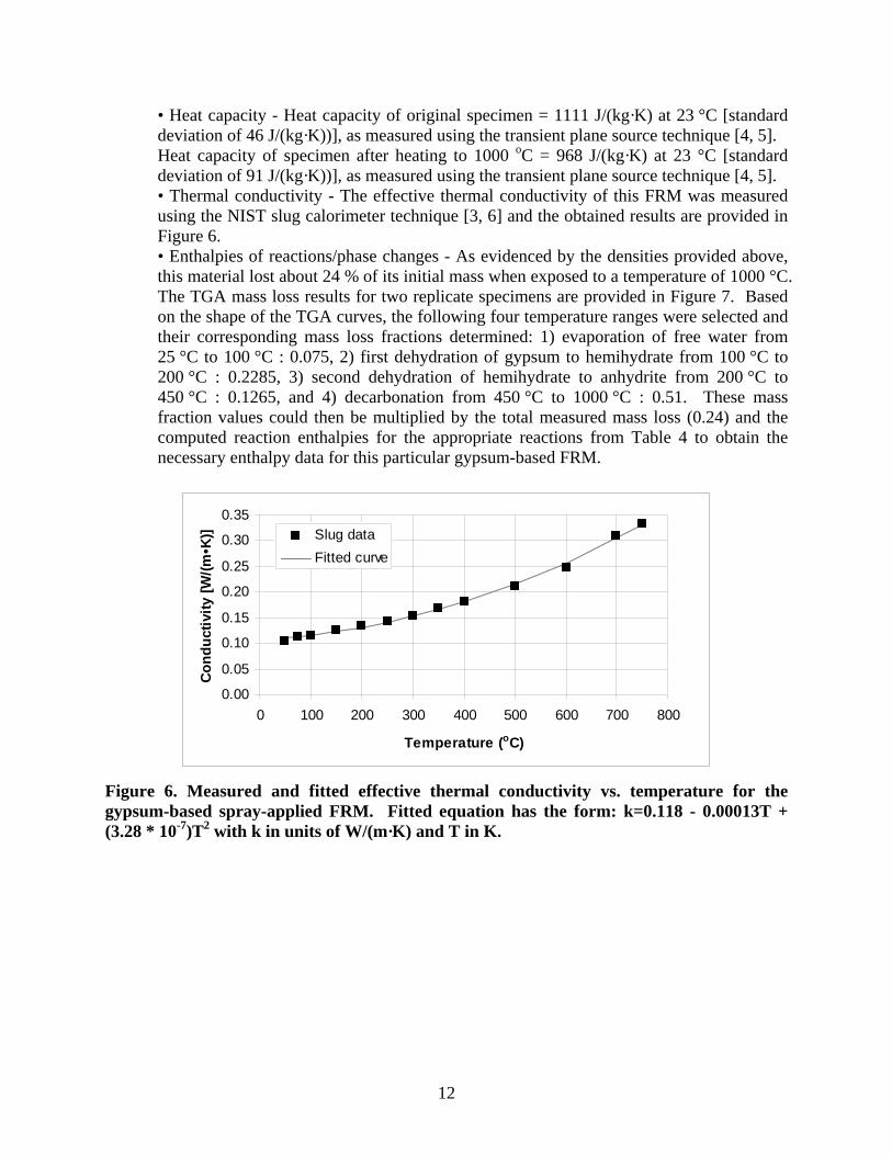
• Thermal conductivity - The effective thermal conductivity of this FRM was measured using the NIST slug calorimeter technique [3, 6] and the obtained results are provided in Figure 6.

• Enthalpies of reactions/phase changes - As evidenced by the densities provided above, this material lost about 24 % of its initial mass when exposed to a temperature of 1000 °C. The TGA mass loss results for two replicate specimens are provided in Figure 7. Based on the shape of the TGA curves, the following four temperature ranges were selected and their corresponding mass loss fractions determined: 1) evaporation of free water from 25 °C to 100 °C : 0.075, 2) first dehydration of gypsum to hemihydrate from 100 °C to 200 °C : 0.2285, 3) second dehydration of hemihydrate to anhydrite from 200 °C to 450 °C : 0.1265, and 4) decarbonation from 450 °C to 1000 °C : 0.51. These mass fraction values could then be multiplied by the total measured mass loss (0.24) and the computed reaction enthalpies for the appropriate reactions from Table 4 to obtain the necessary enthalpy data for this particular gypsum-based FRM.

0.00

0.05

0.10

0.15

0.20

0.25

0.30

0.35

0 100 200 300 400 500 600 700 800

Temperature (oC)

Con

duct

ivity

[W/(m

•K)] Slug data

Fitted curve

Figure 6. Measured and fitted effective thermal conductivity vs. temperature for the gypsum-based spray-applied FRM. Fitted equation has the form: k=0.118 - 0.00013T + (3.28 * 10-7)T2 with k in units of W/(m·K) and T in K.

12

0.0

0.2

0.4

0.6

0.8

1.0

0 100 200 300 400 500 600 700 800 900 1000

Temperature (oC)

Rela

tive

mas

s lo

ss


Figure 7. Relative mass loss vs. temperature for two replicate specimens of the gypsum-based FRM.

3.2.4 Portland Cement-Based (Spray-Applied) Materials

3.2.4.1 Low-density material • Density - Initial density = 224 kg/m3 at 23 °C (laboratory measurement with an expanded

uncertainty of 11 kg/m3 with a coverage factor of 2 [16]) Density after exposure to 1000 °C = 201 kg/m3 at 23 °C (laboratory measurement with an

expanded uncertainty of 10 kg/m3 with a coverage factor of 2 [16]) • Heat capacity - The heat capacity data for this material as a function of temperature was

obtained from reference [6] and is provided in Figure 8. • Thermal conductivity - The effective thermal conductivity of this FRM was measured


• Enthalpies of reactions/phase changes - As evidenced by the densities provided above, this material lost about 11 % of its initial mass when exposed to a temperature of 1000 °C. Previous TGA mass loss results are provided in Figure 10. Based on the shape of the TGA curves, the following four temperature ranges were selected and their corresponding mass loss fractions determined: 1) evaporation of free water from 25 °C to 100 °C : 0.246, 2) dehydration of calcium silicate hydrate from 100 °C to 300 °C : 0.3, 3) dehydration of calcium hydroxide from 300 °C to 600 °C : 0.236, and 4) decarbonation from 600 °C to 1000 °C : 0.218. These mass fraction values could then be multiplied by the total measured mass loss (0.11) and the computed reaction enthalpies for the appropriate reactions from Table 4 to obtain the necessary enthalpy data for this particular portland cement-based FRM.

13

0

200400

600

800

10001200

1400

1600

0 200 400 600 800 1000 1200

Temperature (oC)

Cp [J

/(kg•

K)]

Measured DataFitted curve

Figure 8. Measured values and fitted curve for heat capacity of low density portland cement-based FRM [6]. Fitted equation has the form: Cp=(-263.9) + 0.2736T + 174.1ln(T) with Cp in units of J/(g·K) and T in K.

0.00

0.05

0.10

0.15

0.20

0.25

0.30

0.35

0 100 200 300 400 500 600 700 800

Temperature (oC)

Cond

uctiv

ity [W

/(m•K


Figure 9. Measured and fitted effective thermal conductivity vs. temperature for the low density portland cement-based FRM. Fitted equation has the form: k=0.102 - 0.00024T + (5.05 * 10-7)T2 with k in units of W/(m·K) and T in K.

14

0.80

0.85

0.90

0.95

1.00

0 100 200 300 400 500 600 700 800

Temperature (oC)

Rel

ativ

e M

ass

Measured dataFitted curve

Figure 10. Mass loss vs. temperature for the low density portland cement-based FRM [6].

3.2.4.2 High-density material • Density - Initial density = 768 kg/m3 at 23 °C (laboratory measurement with a standard deviation of

3 kg/m3 based on two replicates) Density after exposure to 1000 °C = 576 kg/m3 at 23 °C (laboratory measurement with an

expanded uncertainty of 30 kg/m3 with a coverage factor of 2 [16]) • Heat capacity - Heat capacity of original specimen = 1295 J/(kg·K) at 23 °C [standard

deviation of 36 J/(kg·K))], as measured using the transient plane source technique [4, 5]. Heat capacity of specimen after heating to 1000 oC = 987 J/(kg·K) at 23 °C [standard

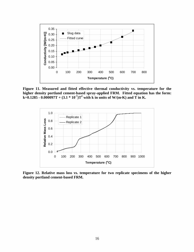
deviation of 31 J/(kg·K))], as measured using the transient plane source technique [4, 5]. • Thermal conductivity - The effective thermal conductivity of this FRM was measured


• Enthalpies of reactions/phase changes - As evidenced by the densities provided above, this material lost about 25 % of its initial mass when exposed to a temperature of 1000 °C. The TGA mass loss results for two replicate specimens are provided in Figure 12. Based on the shape of the TGA curves, the following four temperature ranges were selected and their corresponding mass loss fractions determined: 1) evaporation of free water from 25 °C to 100 °C : 0.073, 2) dehydration of calcium silicate hydrate from 100 °C to 300 °C : 0.282, 3) dehydration of calcium hydroxide from 300 °C to 600 °C : 0.305, and 4) decarbonation from 600 °C to 1000 °C : 0.34. These mass fraction values could then be multiplied by the total measured mass loss (0.25) and the computed reaction enthalpies for the appropriate reactions from Table 4 to obtain the necessary enthalpy data for this particular portland cement-based FRM.

15

0.00

0.05

0.10

0.15

0.20

0.25

0.30

0.35

0 100 200 300 400 500 600 700 800

Temperature (oC)

Cond

uctiv

ity [W

/(m•K


Figure 11. Measured and fitted effective thermal conductivity vs. temperature for the higher density portland cement-based spray-applied FRM. Fitted equation has the form: k=0.1285 - 0.000097T + (3.1 * 10-7)T2 with k in units of W/(m·K) and T in K.

0.0

0.2

0.4

0.6

0.8

1.0

0 100 200 300 400 500 600 700 800 900 1000

Temperature (oC)

Rel

ativ

e M

ass

Loss


Figure 12. Relative mass loss vs. temperature for two replicate specimens of the higher density portland cement-based FRM.

16

4 Simulation of the NIST Slug Calorimeter Experiment The details of the slug calorimeter experimental setup have been provided in references [3] and [6]. The steel slug consists of a 152.4 mm by 152.4 mm by 12.7 mm AISI 304 stainless steel plate into which three thermocouple holes have been milled. It has a mass of 2340 g. The two major faces of the slug are covered with samples of the FRM to be evaluated, each nominally 25 mm thick. The remaining sides of the steel slug (and those of the samples) are surrounded by a high temperature guard insulation material [3, 6]. The assembled specimen is held together by two high temperature retaining plates and a set of eight bolts. When ready for testing, the specimen is placed in a high temperature furnace and exposed to programmed heating/cooling cycles. Generally, the heating cycle is programmed as a series of linear ramps and the cooling is natural (e.g., not imposed). The temperatures of the slug and the sample (exposed) surfaces are monitored and recorded over time. From this temperature/time data, the effective thermal conductivity of the samples as a function of mean sample temperature can be obtained [3, 6]. Here, the slug calorimeter experimental setup will be modeled by a one-dimensional heat transfer model originally developed by Prasad et al. for modeling firefighters’ layered clothing [17]. For a given FRM, data like that provided in Section 3 will be used along with the measured furnace temperatures to simulate the temperature of the steel slug as a function of time during a single complete heating/cooling cycle. Both the 1st (reactions present) and the 2nd (no further reactions occurring) heating/cooling cycles can be simulated in the developed approach. The latter case is simpler as no heat is being generated/consumed by reactions and little if any mass transfer of hot reaction gases (steam) should be occurring. More details and numerous examples of simulations of both the first and second heating/cooling cycles will be provided in the upcoming part II of this NISTIR series. In Figures 13 and 14, the results obtained for a typical FRM during only the second heating/cooling cycle of a slug calorimeter experiment are presented to demonstrate the potential of the simulation model and the adequacy of the property characterization. Excellent agreement between model and experiment is observed for both the FRM exterior surface temperature (Figure 13) and the steel slug temperature (Figure 14) vs. time.

17

0

200

400

600

800

1000

0 300 600 900 1200 1500

Time (min)

Ext

erio

r FR

M te

mpe

ratu

re (

o C)

SimulationSlug experiment

Figure 13. Model-predicted and experimental exterior FRM surface temperature vs. time for a typical FRM during the 2nd heating/cooling cycle of a slug calorimeter experiment.

0

200

400

600

800

0 300 600 900 1200 1500

Time (min)

Slu

g te

mpe

ratu

re (

o C) SimulationSlug experiment

Figure 14. Model-predicted and experimental stainless steel slug temperature vs. time for a typical FRM during the 2nd heating/cooling cycle of a slug calorimeter experiment.

18

5 Prospectus and Future Improvements While the presented thermal property characterization coupled to the one-dimensional thermal modeling have demonstrated the capability to predict thermal performance (e.g., slug temperatures vs. time), additional complications remain to be addressed. One of these is the dramatic expansion that occurs when intumescent materials are exposed to a fire. Here, both the experimental measurement of thickness as a function of temperature and the computational ability to “re-grid” the one-dimensional model during its execution will likely be required to enable an accurate prediction of thermal performance. Another challenge will be the incorporation of mass (steam and gas) transfer. From an experimental viewpoint, measurements of both liquid and gas permeability of the FRMs as a function of temperature may be needed. Modeling of combined heat/mass transfer adds an additional layer of complexity; however, the firefighter clothing model has already been formulated with this in mind [17]. Similar issues have been raised previously in the simulation of the fire performance/spalling of (high-performance) concrete [18]. Ultimately, the methodologies demonstrated in this report should be equally applicable to simulating a priori the performance of these FRMs in ASTM E119 fire tests and even in actual (well characterized) fires. Conversely, it may also be possible to extract fundamental thermophysical property information from temperatures measured during an E119 fire test, as first proposed by Wickström over 20 years ago [19].

19

6 Acknowledgements The authors would like to acknowledge the financial and technical support of the industrial members of the National Institute of Standards and Technology/industry consortium on Performance Assessment and Optimization of Fire Resistive Materials: the American Iron and Steel Institute, Anter Corporation, Barrier Dynamics LLC, Isolatek International, LightConcrete LLC, PPG Industries, and W.R. Grace & Co.- Conn.

7 References [1] ASTM, ASTM Annual Book of Standards, ASTM International, West Conshohocken 2007. [2] Bentz, D.P., Prasad, K.R., and Yang, J.C., “Towards a Methodology for the Characterization

of Fire Resistive Materials with Respect to Thermal Performance Models,” Fire and Materials, Vol. 30, 311-321 (2006).

[3] Bentz, D.P., “Combination of Transient Plane Source and Slug Calorimeter Measurements to Estimate the Thermal Properties of Fire Resistive Materials,” Journal of Testing and Evaluation, Vol. 35 (3), (2007).

[4] Gustafsson, S.E., “Transient Plane Source Techniques for Thermal Conductivity and Thermal Diffusivity Measurements of Solid Materials,” Review of Scientific Instruments, Vol. 62 (3), 797-804 (1991).

[5] Log, T., and Gustaffson, S.E., “Transient Plane Source (TPS) Technique for Measuring Thermal Transport Properties of Building Materials,” Fire and Materials, Vol. 19, 43-49 (1995).

[6] Bentz, D.P., Flynn, D.R., Kim, J.H., and Zarr, R.R., “A Slug Calorimeter for Evaluating the Thermal Performance of Fire Resistive Materials,” Fire and Materials, Vol. 30 (4), 257-270 (2006).

[7] CRC Handbook of Chemistry and Physics, 68th edition (CRC Press, Boca Raton, FL, 1987). [8] Smith, J.M., and Van Ness, H.C., Introduction to Chemical Engineering Thermodynamics

(McGraw-Hill, New York, 1975). [9] Taylor, H.F.W., Cement Chemistry, 2nd edition (Thomas Telford, London, 1997). [10] Hansen, P.F., Hansen, J., Hougaard, K.V., and Pedersen, E.J., “Thermal Properties of

Hardening Cement Paste,” in Proceedings of the RILEM International Conference on Concrete at Early Ages (RILEM, Paris, 1982) pp. 23-26.

[11] Thomas, G., “Thermal Properties of Gypsum Plasterboard at High Temperatures,” Fire and Materials, Vol. 26, 37-45 (2002.)

[12] Bogaard R.H., Desai P.D., Li H.H., and Ho C.Y., “Thermophysical Properties of Stainless Steels,” Thermochimica Acta, Vol. 218, 373-393 (1993).

[13] Bogaard, R.H., “Thermal Conductivity of Selected Stainless Steels,” in Thermal Conductivity 18, Proceedings of the Eighteenth International Conference on Thermal Conductivity, Eds. T. Ashworth and D.R. Smith (Plenum, New York, 1985) pp. 175-185.

[14] Sweet, J.N., Roth, E.P., and Moss, M., “Thermal Conductivity of Inconel 718 and 304 Stainless Steel,” International Journal of Thermophysics, Vol. 8 (5), 593-606 (1987).

20

[15] Gayle, F.W., Fields, R.J., Luecke, W.E., Banovic, S.W., Foecke, T., McGowan, C.N., Siewert, T.A., and McColskey, J.D., “Mechanical and Metallurgical Analysis of Structural Steel,” NIST NCSTAR 1-3 Federal Building and Fire Safety Investigation of the World Trade Center Disaster, U.S. Department of Commerce, September 2005.

[16] Taylor, B.N., and Kuyatt, C.E., “Guidelines for Evaluating and Expressing the Uncertainty of NIST Measurement Results,” NIST Technical Note 1297, U.S. Department of Commerce, 1994.

[17] Prasad, K., Twilley, W., and Lawson, J.R., “Thermal Performance of Fire Fighters’ Protective Clothing. 1. Numerical Study of Transient Heat and Water Vapor Transfer,” NISTIR 6881, U.S. Department of Commerce, August 2002.

[18] Phan, L.T., Carino, N.J., Duthinh, D., and Garboczi, E.J. (eds.), “International Workshop on Fire Performance of High-Strength Concrete, NIST, Gaithersburg, MD, February 13-14, 1997 Proceedings,” NIST Special Publication 919; 174 p. September 1997.

[19] Wickström, Y., “Temperature Analysis of Heavily-Insulated Steel Structures Exposed to Fire,” Fire Safety Journal, Vol. 5, 281-285 (1985).

21

thermal performance of fire resistive materials

Documents