theory of multiobjective optimization - khoa toánnvthuy/om/theoryofmultiobjectiveoptimiz… ·...
TRANSCRIPT

THEORY OFMULTIOBJECTIVEOPTIMIZATION

This is Volume 176inMATHEMATICS IN SCIENCE AND ENGINEERINGA Series of Monographs and TextbooksEdited by RICHARD BELLMAN, University of Southern California
The complete listing of books in this series is available from the Publisher upon request.

THEORY OFMULTIOBJECTIVEOPTIMIZATION
YOSHIKAZU SAWARAGI
Faculty of ScienceThe Kyoto Sangyo UniversityKyoto, Japan
HIROTAKA NAKAYAMA
Department of Applied MathematicsKonan UniversityKobe, Japan
TETSUZO TANINO
Department of Mechanical Engineering IITohoku UniversitySendai, Japan
Academic Press, Inc.(Harcourt Brace Jovanovich, Publishers)
Orlando SanDiego New York LondonToronto Montreal Sydney Tokyo
COPYRIGHT © 1985, BY ACADEMIC PREss, INC.ALL RIGHTS RESERVED.NO PART OF THIS PUBUCATION MAY BE REPRODUCED ORTRANSMITTED IN ANY FORM OR BY ANY MEANS, ELECTRONICOR MECHANICAL, INCLUDING PHOTOCOPY, RECORDING, ORANY INFORMATION STORAGE AND RETRIEVAL SYSTEM, WITHOUTPERMISSION IN WRITING FROM THE PUBUSHER.
ACADEMIC PRESS, INC.Orlando, Florida 32887
United Kingdom Edition published byACADEMIC PRESS INC. (LONDON) LTD.24-28 Oval Road, London NWI 7DX
Library of Congress Cataloging in Publication Data
Sawaragi, Yoshikazu, DateTheory of multiobjective optimization.
Includes index.I. Mathematical optimization. I. Nakayama,
Hirotaka, Date. II. Tanino, Tetsuzo.III. Title.QA402.5.S28 1985 519 84-14501ISBN 0-12~620370-9 (alk. paper)
PRINTED IN THE UNITED STATES OF AMERICA
85 86 87 88 987654321

To our wivesAtsumi, Teruyo, and Yuko

This page intentionally left blank
CONTENTS
PrefaceNotation and Symbols
1 INTRODUCTION
2 MATHEMATICAL PRELIMINARIES
2.1 Elements of Convex Analysis2.2 Point-To-Set Maps2.3 Preference Orders and Domination Structures
3 SOLUTION CONCEPTS AND SOME PROPERTIES OFSOLUTIONS
3.1 Solution Concepts3.2 Existence and External Stability of Efficient Solutions3.3 Connectedness of Efficient Sets3.4 Characterization of Efficiencyand Proper Efficiency3.5 Kuhn-Tucker Conditions for Multiobjective Programming
4 STABILITY
4.1 Families of Multiobjective Optimization Problems4.2 Stability for Perturbation of the Sets of Feasible Solutions4.3 Stability for Perturbation of the Domination Structure4.4 Stability in the Decision Space4.5 Stability of Properly Efficient Solutions
vii
ixxi
62125
3247667089
9294
107119122

viii CONTENTS
5 LAGRANGE DUALITY
5.1 Linear Cases5.2 Duality in Nonlinear Multiobjective Optimization5.3 Geometric Consideration of Duality
6 CONJUGATE DUALITY
6.1 Conjugate Duality Based on Efficiency6.2 Conjugate Duality Based on Weak Efficiency6.3 Conjugate Duality Based on Strong Supremum and Infimum
7 METHODOLOGY
7.1 Utility and Value Theory7.2 Stochastic Dominance7.3 Multiobjective Programming Methods
References
Index
127137148
167190201
210244252
281
293

PREFACE
This book presents in a comprehensive manner some salient theoreticalaspects of multiobjective optimization. The authors had been involved inthe special research project Environmental Science, sponsored by theEducation Ministry of Japan, for more than a decade since 1970. Throughthe research activities, we became aware that an important thing is notmerely to eliminate pollutants after they are discharged, but how to createa good environment from a holistic viewpoint. What, then, is a goodenvironment? There are many factors: physical, chemical, biological,economic, social, and so on. In addition, to make the matter more difficult,there appear to be many conflicting values.
System scientific methodology seems effective for treating such a multi-plicity of values. Its main concern is how to trade off these values. One ofthe major approaches is multiobjective optimization. Another is multi-attribute utility analysis. The importance of these research themes hasbeen widely recognized in theory and practice. Above all, the workshops atSouth Carolina in 1972 and at IIASA in 1975 have provided remarkableincentives to this field of research. Since then, much active research hasbeen observed all over the world.
Although a number of books in this field have been published in recentyears, they focus primarily on methodology. In spite of their importance,however, theoretical aspects of multiobjective optimization have neverbeen dealt with in a unified way.
In Chapter 1 (Introduction), fundamental notions in multiobjectivedecision making and its historical background are briefly explained.Throughout this chapter, readers can grasp the purpose and scope of thisvolume.
Chapters 2-6 are the core of the book and are concerned with the mathe-matical theories in multiobjective optimization of existence, necessary and
ix

x PREFACE
sufficient conditions of efficient solutions, characterization of efficientsolutions, stability, and duality. Some of them are still developing, but wehave tried to describe them in a unified way as much as possible.
Chapter 7 treats methodology including utility/value theory, stochasticdominance, and multiobjective programming methods. We emphasizedcritical points of these methods rather than a mere introduction. We hopethat this approach will have a positive impact on future development ofthese areas.
The intended readers of this book are senior undergraduate students,graduate students, and specialists of decision making theory and mathe-matical programming, whose research fields are applied mathematics,electrical engineering, mechanical engineering, control engineering, econo-mics, management sciences, operations research, and systems science. Thebook is self-contained so that it might be available either for reference andself-study or for use as a classroom text; only an elementary knowledge oflinear algebra and mathematical programming is assumed.
Finally, we would like to note that we were motivated to write this bookby a recommendation of the late Richard Bellman.

NOTATION AND SYMBOLS
X:=yXES
xrtSSCclSint SasSeT, T => SSu TS (l TS\TS+ T
S x T
x is defined as yx is a member of the set Sx is not a member of the set Scomplement of the set Sclosure of the set Sinterior of the set Sboundary of the set SS is a subset of the set Tunion of two sets Sand Tintersection of two sets Sand Tdifference between Sand T, i.e., S (l TCsum of two sets Sand T,i.e., S + T:= {s+ t: s E S
and tE T}Cartesian product of the sets Sand T, i.e.,
S x T:= {(s, t): s E Sand t E T}n-dimensional Euclidean space. A vector x in R"
is written x = (Xl' X 2' ••. , x n) , but whenused in matrix calculations it is representedas a column vector, i.e.,
The corresponding row vector is x T = (x., x 2 ,
... ,xn). When A = (a i) is an m x n matrixwith entry aij in its ith row andjth column, the
xi
xii
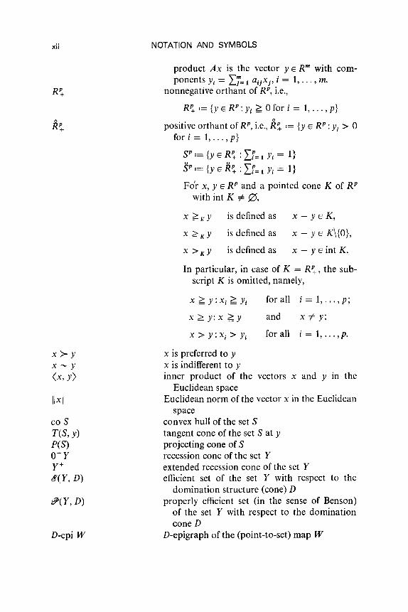
RP+
x>yX-Y<x,Y)
[x]
co ST(S, y)P(S)O+yy+
@,(Y, D)
.9(Y, D)
D-epi W
NOTATION AND SYMBOLS
product Ax is the vector Y E R" with com-ponents Yi = Ij= 1 aijxj , i = 1, ... , m.
nonnegative orthant of RP, i.e.,
R~ := {y E RP:Yi ~ 0 for i = 1, ... , p}
positive orthant of RP, i.e., R~ := {y E RP:Yj > 0fori=1, ... ,p}
SP:={YER~:If=lYi= 1}
SP := {y E R~ :If= 1 Yi = l}
Fo'r x, y E RP and a pointed cone K of RPwith int K =1= 0,
x ~ K Y is defined as x - Y E K,
x ~ K Y is defined as x - y E K\{O},
x > K Y is defined as x - Y E int K.
In particular, in case of K = R~, the sub-script K is omitted, namely,
x ~ y:xi ~ Yi for all i= 1, ... , p;
x ~ y:x ~y and x =1= Y;
x> y t x, > Yi for all i = 1,oo.,p.
x is preferred to Yx is indifferent to Yinner product of the vectors x and Y in the
Euclidean spaceEuclidean norm of the vector x in the Euclidean
spaceconvex hull of the set Stangent cone of the set S at Yprojecting cone of Srecession cone of the set Yextended recession cone of the set Yefficient set of the set Y with respect to the
domination structure (cone) Dproperly efficient set (in the sense of Benson)
of the set Y with respect to the dominationconeD
D-epigraph of the (point-to-set) map W

NOTATION AND SYMBOLS xiii
b(·IS)f'(x; d)
Vf(x)
f*F*F**(f**)af(x)
aF(x; y)Maxj, Y (MinD Y)
w-Maxj, Y (w-Min., Y)
w-Sup Y(w-Inf Y)
w-F*w-F**w-aF(x)
w-Lmax Y (min Y)sup Y (inC Y)f*of(x)
indicator function of the set Sone-sided directional derivative of the functionf
at xgradient of the function f at x, i.e., iff: R" -lo R,
Vf(x) .= (af(x) , af(x) , ... , af(x»)aX 1 ax z ox"
conjugate map (or function) of the functionfconjugate map of the point-to-set map Fbiconjugate map of F(f)subdifferential of the (vector-valued) function
fat xsub differential of the point-to-set map F at (x; y)set of the D-maximal (D-minimal) points of the
set Y, i.e., Maxj, y.= 8'(Y, -D) (Min., y.=8(Y, D». In case of D = R~, in particular,Max y.= 8(Y, -R~) (Min y.= 8'(Y, R~»
set of the weak D-maximal (D-minimal) pointsof the set Y. In case of D = R~, in particular,the subscript D is omitted.
set of the weak supremal (infimum) points of theset Y
weak conjugate map of the point-to-set map Fweak biconjugate map of the point-to-set map Fweak subdifferential of the point-to-set map F
at xweak Lagrangianstrong maximum (minimum) of the set Ystrong supremum (infimum) of the set Ystrong conjugate of the vector-valued functionfstrong subdifferential of the vector-valued func-
tionfat x

This page intentionally left blank
1 INTRODUCTION
Every day we encounter various kinds of decision making problems asmanagers, designers, administrative officers,mere individuals, and so on. Inthese problems, the final decision is usually made through several steps, eventhough they sometimes might not be perceived explicitly. Figure 1.1 shows aconceptual model of the decision making process. It implies that the finaldecision is made through three major models, the structure model, the impactmodel, and the evaluation model.
By structure modeling, we mean constructing a model in order to know thestructure of the problem, what the problem is, which factors comprise theproblem, how they interrelate, and so on. Through the process, the objectiveofthe problem and alternatives to perform it are specified. Hereafter, we shalluse the notation (!) for the objective and X for the set of alternatives, which issupposed to be a subset of an n-dimensional vector space. If we positivelyknow a consequence caused by an alternative, the decision making is said tobe under certainty; whereas if we cannot know a sure result because of someuncertain factor(s), the decision making is said to be under uncertainty.Furthermore, if we objectively or subjectively know the probability distri-bution of the possible consequences caused by an alternative, the decisionmaking is said to be under risk. Even though the final objective might be asingle entity, we encounter, in general, many subobjectives (!)i on the way tothe final objective. In this book, we shall consider decision making problemswith multiple objectives. Interpretive structural modeling (ISM) (Warfield[W5]) can be applied effectivelyin order to obtain a hierarchical structure ofthe objectives.
In order to solve our decision making problem by some systems-analyticalmethods, we usually require that degrees of objectives be represented innumerical terms, which may be of multiple kinds even for one objective. In
1

2
Problem
INTRODUCTION
Fil!:.1.1. Conceptual model of the decision making process.
Decision
order to exclude subjective value judgment at this stage, we restrict thesenumerical terms to physical measures (for example, money, weight, length,and time). As such a performance index, or criterion, for the objective (9;, anobjective function J;:X -+ R 1 is introduced, where R 1 denotes one-dimensional Euclidean space. The value J;(x) indicates how much impact isgiven on the objective (9; by performing an alternative x. Impact modeling isperformed to identify these objective functions from various viewpoints suchas physical, chemical, biological, social, economic, and so on. For con-venience of mathematical treatment, we assume in this book that a smallervalue for each objective function is preferred to a larger one. Now we canformulate our decision making problems as a multiobjective optimizationproblem:
(P) Minimize over x EX.
This kind of problem is also called a vector optimization. In some cases, someof the objective functions are required to be maintained under given levelsprior to minimizing other objective functions. Denoting these objectivefunctions by gix), we require that
gJ{x) ::;; 0, j = 1, ... , m,
which, for convenience, is also supposed to represent some other technicalconstraints. Such a function gix) is generally called a constraint function inthis book. According to the situation, we will consider either the problem (P)itself or (P) accompanied by the constraint gix) ::;; 0 U= 1, ... , m). Ofcourse, an equality constraint hk(x) = 0 can be embedded within twoinequalities hix)::;; 0 and - hk(x) ::;; 0, and, hence, it does not appearexplicitly in this book.
Unlike traditional mathematical programming with a single objectivefunction, an optimal solution in the sense of one that minimizes all theobjective functions simultaneously does not necessarily exist in multiobjec-tive optimization problems, and, hence, we are troubled with conflicts amongobjectives in decision making problems with multiple objectives. The finaldecision should be made by taking the total balance of objectives intoaccount. Therefore, a new problem of value judgment called value trade-offarises. Evaluation modeling treats this problem that is peculiar to decision

INTRODUCTION 3
making with multiple objectives. Here we assume a decision maker who isresponsible for the final decision. In some cases, there may be many decisionmakers, for which cases the decision making problems are called groupdecision problems. We will consider cases with a single decision maker in thisbook. The decision maker's value is usually represented by saying whether ornot an alternative x is preferred to another alternative x', or equivalentlywhether or not f(x) is preferred to f(x'). In other words, the decision maker'svalue is represented by some binary relation defined over X or f(X). Sincesuch a binary relation representing the decision maker's preference usuallybecomes an order, it is called a preference order. In this book, the decisionmaker's preference order is supposed to be defined on the so-called criteriaspace Y, which includes the setf(X). Several kinds of preference orders will bepossible, sometimes, the decision maker cannot judge whether or not f(x) ispreferred to f(x'). Roughly speaking, such an order that admits incom-parability for a pair of objects is called a partial order, whereas the orderrequiring the comparability for every pair of objects is called a weak order (ortotal order). In practice, we often observe a partial order for the decisionmaker's preference. Unfortunately, however, an optimal solution in the senseof one that is most preferred with respect to the order, whence the notion ofoptimality does not necessarily exist for partial orders. Instead of strictoptimality, we introduce in multiobjective optimization the notion ofefficiency. A vector f(x) is said to be efficient if there is no f(x) (x E X)preferred to f(x) with respect to the preference order. The final decision isusually madeamong the set of efficient solutions. --,'
One approach to evaluation modeling is to find a scalar-valued functionU(fl' ... ,Jp) representing the decision maker's preference, which is called apreference function in this book. A preference function in decision makingunder risk is called a utility function, whereas the one in decision makingunder certainty is called a value function. The theory regarding existence,uniqueness, and practical representation of such a utility or value function iscalled the utility and value theory. Once we obtain such a preference function,our problem reduces to the traditional mathematical programming:
Maximize over x E X.
Another popular approach is the interactive programming that performsthe solution search and evaluation modeling. In this approach, the solution issearched without identifying the preference function by eliciting iterativelysome local information on the decision maker's preference.
Kuhn and Tucker [KlO] first gave some interesting results concerningmultiobjective optimization in 1951. Since then, research in this field hasmade remarkable progresss both theoretically and practically. Some of theearliest attempts to obtain conditions for efficiency were carried out by Kuhn
4 INTRODUCTION
and Tucker [KlO], and Arrow et al. [A5]. Their research has been inheritedby Da Cunha and Polak [01], Neustadt [N14], Ritter [R4-R6], Smale [SlO,S11], Aubin [A7], and others. After the 1970s,practical methodology such asutility and value analysis and interactive programming methods have beenactively researched as tools for supporting decision making, and many booksand conference proceedings on this topic have been published. (See, forexample, Lee [Ll], Cochrane and Zeleny [C12], Keeney and Raiffa [K6],Leitmann and Marzollo [L3], Leitmann [L2], Wilhelm [W15], Zeleny [Z4-Z6], Thiriez and Zionts [T14], Zionts [Z7], Starr and Zeleny [S13],Nijkamp and Delft [N18], Cohon [C13], Hwang and Masud [H17],Salkuvadze [S3], Fandel and Gal [F2], Rietveld [R3], Hwang and Yoon[H18], Morse [M5], Goicoeche et al. [G8], Hansen [H3], Chankong andHaimes [C6], and Grauer and Wierzbicki [GlO].)
On the other hand, duality and stability, which play an important rolein traditional mathematical programming, have been extended to multi-objective optimization since the late 19708. Isermann [15-17] developedmultiobjective duality in the linear case, while the results for nonlinear caseshave been given by Schonfeld [S6], Rosinger [R10], Guglielmo [G 12],Tanino and Sawaragi [T9, T11], Mazzoleni [M3], Bitran [B13], Brumelle[B21], Corley [C16], Jahn [11], Kawasaki [K2, K3], Luc [LlO], Nakayama[NS], and others. Stability for multiobjective optimization has been de-veloped by Naccache [N2] and Tanino and Sawaragi [TlO].
This book will be mainly concerned with some of the theoretical aspects inmultiobjective optimization; in particular, we will focus on existence, neces-sary/sufficient conditions, stability, Lagrange duality, and conjugate dualityfor efficient solutions. In addition, some methodology such as utility andvalue theory and interactive programming methods will also be discussed.
Chapter 2 is devoted to some mathematical preliminaries. The first sectiongives a brief review of the elements of convex analysis that play an importantrole not only in traditional mathematical programming but also in multi-objective optimization. The second section describes point-to-set maps thatplaya very important role in the theory of multiobjective optimization, sincethe efficient solutions usually constitute a set. The concepts of continuity andconvexity of point-to-set maps are introduced. These concepts are fundamen-tal for existence and necessary/sufficient conditions for efficient solutions.The third section is concerned with a brief explanation of preference orderand domination structures.
Chapter 3 begins with the introduction of several possible concepts forsolutions in multiobjective optimization. Above all, efficient solutions will bethe subject of primary consideration in subsequent theories. Next, someproperties of efficient solutions, such as existence, external stability,connectedness, and necessary/sufficientconditions, will be discussed.

INTRODUCTION 5
Chapter 4 develops the stability theory in multiobjective optimization. Thefactors that specify multiobjective optimization problems are the objectivefunctions with some constraints and the preference structure of the decisionmaker. Therefore, the stability of the solution set for perturbations of thosefactors is considered by using the concept of continuity of the solution map(which is a point-to-set map). A number of illustrative examples will beshown.
Chapter 5 will be devoted to the duality theory in multiobjective optimi-zation. Duality is a fruitful result in traditional mathematical programmingand is very useful both theoretically and practically. Consequently, it is quiteinteresting to extend the duality theory to the case of multiobjectiveoptimization. In this chapter, the duality of linear multiobjective optimi-zation will be introduced. Next, a more general duality theory for nonlinearcases will be discussed in parallel with the case of ordinary convexprogramming. Given a convex multiobjective programming problem, somenew concepts such as the primal map, the dual map, and the vector-valuedLagrangian will be defined. The Lagrange multiplier theorem, the saddle-point theorem, and the duality theorem will be obtained via geometricconsideration.
Chapter 6 will develop the conjugate duality theory in multiobjectiveoptimization. Rockafellar [R8] constructed a general and comprehensiveduality theory for an ordinary convex optimization problem by embedding itin a family of perturbed problems and associating a dual problem with it byusing conjugate functions. In this chapter, we shall introduce the concept ofconjugate maps, which are extensions of conjugate functions, and developduality for convex multiobjective optimization problems. In addition, recentresults on this topic from several approaches will be introduced.
Chapter 7 deals with the methodology for practical implementation ofmultiobjective optimization. Although various methods for multiobjectiveoptimization have been developed, we shall focus on some of the mainapproaches (for example, the ultility and value theory and interactiveprogramming methods). However, our aim is not merely to introduce thesemethods, but to clarify the noticeable points about them. In the first section,the utility and value theory will be treated. There, we shall introduce severalresults on existence, uniqueness, and representation of preference functionsthat represent the decision maker's preference. Several practical implicationsof these methods, in particular, von Neumann-Morgenstern utility functions,will also be discussed along with clarification of some of their controversialpoints. In the next section, we shall discuss interactive programmingmethods, showing some typical methods as examples. Desirable properties ofthis approach will be clarified throughout the discussion.
2 MATHEMATICAL PRELIMINARIES
This chapter is devoted to mathematical preliminaries. First, some fun-damental results in convex analysis, mainly according to Rockafellar [R7],are reviewed. Second, the concepts of continuity and convexity of vector-valued point-to-set maps are introduced. Finally, the concepts of preferenceorders, domination structures, and nondominated solutions are introducedto provide a way of specifying solutions for multiobjective optimizationproblems.
2.1 Elements of Convex Analysis
As is well known, convexity plays an important role in the theory ofoptimization with a single objective. A number of books dealing with convexoptimization both in finite and infinite dimensional spaces have beenpublished (Rockafellar [R7], Stoer and Witzgall [SI5], Holmes [HI2],Bazaraa and Shetty [B3], Ekeland and Temam [EI], Ioffe and Tihomirov[14], Barbu and Precupanu [BI], and Ponstein [P2]).
Since they are also fundamental in the theory of multiobjective optimi-zation, some elementary results are summarized below. All spaces consideredare finite-dimensional Euclidean spaces. The fundamental text for thissection is "Convex Analysis" by Rockafellar [R7], and the reader might referto it for details.
2.1.1 Convex Sets
In this subsection, we will first look at convex sets, which are fundamentalin convex analysis.
6

2.1 ELEMENTS OF CONVEX ANALYSIS
Definition 2.1.1 (Convex Set)
A subset X of R" is said to be convex if
7
for any XI,X2
E X and any rt E [0,1].
Proposition 2.1 .1
A subset X of R" is convex if and only if x; E X (i = 1, ... , k), rt; ~ 0(i = 1, ... , k), and L~=l rt; = 1 imply L~=l rt;X
i EX; that is, if and only if itcontains all convex combinations of its elements.
Definition 2.1.2 (Convex Hull)
The intersection of all the convex sets containing a given subset X of R" iscalled the convex hull of X and is denoted by co X.
Proposition 2.1.2
(i) co X is the unique smallest convex set containing X.(ii) co X = {L~=l rtiX
i: rti ~ 0, L~=l rti = 1, Xi E X (i = 1, ... , k)};
that is, co X consists of all the convex combinations of the elements of X.
Definition 2.1.3 (Cone and Convex Cone)
A subset K of R" is called a cone if rtX E K whenever x E K and rt > O.Moreover, a cone K is said to be a convex cone when it is also convex.
Proposition 2.1 .3
A set K in R" is a convex cone if and only if
(i) x E K and rt > 0 imply eoc E K,(ii) x ', x 2 E K imply x' + Xl E K.
Definition 2.1.4 (Pointed Cone and Acute Cone)
A cone K c R" is said to be pointed if -x 1= K when x # 0 and x E K. Inother words, K is pointed if it does not contain any nontrivial subspaces. It issaid to be acute if there is an open halfspace (see Definition 2.1.16)
fI+ = {x E R":<x, x*) > O} x* # 0
such that
elK c fI+ u {OJ.

8 2 MATHEMATICAL PRELIMINARIES
Proposition 2.1.4
When K is a convex cone, it is acute if and only if cl K is pointed.
Of course, acuteness is a stronger concept than pointedness. If K is closedand convex, these concepts coincide.
Definition 2.1.5 (Polar and Strict Polar)
For a subset X in R", its positive polar XO is defined by
X O = {x* ERn: <x,x*) ~ 0 for any x EX}.
The strict positive polar XSO of X is defined by
X'O = {x* ERn: <x, x*) > 0 for any nonzero x EX}.
Proposition 2.1.5
Let X, Xl' and X 2 be sets in Rn. Then
(i) the polar XO is a closed convex cone,(ii) the strict polar X'" is a convex cone,
(iii) XO = (el X)O,(iv) if X is open, X'O u {O} = Xc,(v) Xl C X 2 implies X~ C X~ and X~o c xs
lo, and(vi) if K is a nonempty convex cone, K oo = cl K.
Proposition 2.1.6
Let K I and K 2 be cones in R". Then
(i) if K 1 and K 2 are nonempty,
(K I + K 2 )O = K~ n K~ = (K I U K 2)O,
(ii) (K I n K 2)O :::> K~ + K~ = co(K~ u K~),
(iii) if K I and K 2 are closed convex with nonempty intersection,
(K 1 n K 2 )O= cl(K~ + K~) = cl co(K~ u Kn.If ri K I n ri K 2 i' 0, in addition, then
(K I r. K 2)O = K~ + K~.
Furthermore, the last equality holds also for convex polyhedral cones(Definition 2.1.7) K 1 and K 2 •
2.1 ELEMENTS OF CONVEX ANALYSIS 9
Proposition 2.1.7 t
Let K be a cone in W. Then
(i) int KO #- 0 if and only if K is acute,(ii) when K is acute, int KO = (cl Kro.
Proof
(i) Suppose first that int KO #- 0. Let x* #- 0 in int KO and fr ={x E R": (x, x*) > OJ. We now show that cl K c fr u {OJ. Suppose, to thecontrary, that (x, x*) ~ 0 for some nonzero x E cl K. Since x* E int KO,x* - IXX E KO for sufficiently small IX > O. Since KO = (cl K)O [Proposition2.1.5 (iii)],
<x, x* - IXX) ~ O.
However, this implies that <x, x*) ~ IX<X, x) > 0, which contradicts thehypothesis <x,x*) ~ O. Hence, cl K c fr u {OJ.
Conversely, suppose that K is acute, i.e., cl K c fr u {OJ ={x E R": <x, x*) > O} u {OJ for some x* #- 0 E W. We now prove thatx* E int KO. Ifwe suppose the contrary, there exist sequences {x'"} C R" and{x"} c K such that
X*k --+ x* and <x\ X*k) < 0 for all k.
We may assume without loss of generality that Ilxkll = 1 for all k and soxk
--+ x for some x E cl K with Ilxll = 1. Clearly then <x\ X*k) --+
(x, x*) ~ O. However, this contradicts the fact that cl K c ir u {OJ.(ii) The inclusive relation int KO c (cl Kyo holds whether K is acute or
not. In fact, let x* E int KO, and suppose that x* ¢ (cl Kyo. Then there existsnonzero x' E cl K such that <x', x*) ~ 0. Since x* - lXX' E KO = (cl Kt forsufficiently small IX > 0, then
(x', x*) = <x', x* - IXX') + IX<X', x') > 0,
which is a contradiction.To prove the converse, let x* ¢ int KO. Then there exist sequences
{X*k} C Wand {x'} c K such that
X*k --+ x* and <x\ X*k) < 0 for all k.
We may assume without loss of generality that II~II = 1 and so xk--+ x for
some x E cl K with Ilxll = 1. Then clearly <x\ X*k) --+ (x,x*) ~ 0. Thisimplies that x* rt (cl Kro, which is what we wished to prove.
tyu [VI].
10 2 MATHEMATICAL PRELIMINARIES
Proposition 2.1.8t
Let K 1 be a nonempty, closed, pointed convex cone and K 2 be anonempty, closed, convex cone. Then
(-K 1 ) n K 2 = {OJ
if and only if
K~O n K~ =f- 0.Proof First suppose that there exists x* E KS10 n K~. Then, for any
nonzero x E ( - K 1) n K 2 ,
<-x, x*) > 0 and <x, x*) ~ 0,
which is impossible. Therefore (-K 1 ) n K 2 = {OJ. (Note that 0 is alwayscontained in (- K 1) n K 2 because both K 1 and K 2 are nonempty closedcones.)
Conversely, suppose that K~o n K~ = 0. Then, by the separationtheorem of convex sets (Theorem 2.1.1), there exist x =f- 0 E Wand f3 E Rsuch that
<x, x*) ~ f3
<x,x*) ~ f3
for any x* E K~o,
for any x* E K~.
Since both K~o and K 2 are cones, f3 should be equal to O. Hence,
x E [-(K~O)oJ n (K~)o.
From Propositions 2.1.5 and 2.1.7,
(K~O)O = (int K~)O = (K~)O = cl K 1 = K 1,
and from Proposition 2.1.5 (vi),
Therefore, x E (-K 1) n K 2 , i.e., (-K 1) n K 2 =f- {OJ.
Definition 2.1.6 (Recession Cone)
Let X be a convex set in R". Its recession cone 0+X is defined by
O+X = {x' E R": x + ax' E X for any x E X and a > OJ.
Of course, 0+X is a convex cone containing the origin.
t Borwein [B17] and Bitran and Magnanti [B14].
Proposition 2.1.9
2.1 ELEMENTS OF CONVEX ANALYSIS 11
If {Xi: i E I} is an arbitrary collection of closed convex sets in R" whoseintersection is not empty, then
Proposition 2.1.10
A nonempty closed convex set X in R" is bounded if and only if itsrecession cone O+X = {OJ.
Proposition 2.1.11
Let Xl and X 2 be nonempty closed convex sets in R", If
0+X1 n (-0+X 2 ) = {OJ,
then the set XI + X 2 is closed, and
0+(X1 + X 2 ) = 0+X1 + 0+X2 •
Definition 2.1.7 (Polyhedral Convex Set and Polyhedral Convex Cone)
A set X in R" is said to be a polyhedral convex set if it can be expressed asthe intersection of some finite collection of closed halfspaces (see Definition2.1.16), i.e., if
X = {x: <bi, x) ~ Pi (i = 1, ... , mn,where bi E R" and Pi E R (i = 1, ... ,m). If Pi = 0 for all i = 1, ... ,m in theabove expression, X is said to be a polyhedral convex cone.
Definition 2.1.8 (Finitely Generated Convex Set and Finitely GeneratedConvex Cone)
A set X in R" is said to be a finitely generated convex set if there existvectors ai, a2, ••• , am such that for a fixed integer k (0 ~ k ~ m), X can beexpressed as
X= {x:x = f (lid, (Xi ~ 0(i = 1, ... ,m), ±(Xi = 1}.i~l i=1

12 2 MATHEMATICAL PRELIMINARIES
If X can be expressed as
X = {x : x = .f (Xi a; (Xi ~ 0 (i = 1, ... , m)} ,,=1
then X is said to be a finitely generated convex cone and {a1, ••• , am} is called
the set of generators for the cone.
Proposition 2.1.12
A convex set X is polyhedral if and only if it is finitely generated.
Proposition 2.1.13
The polar of a polyhedral convex set is also polyhedral. In particular, if
X = {X: <bi,x) ~ 0 (i = 1, ... , m)},
then its polar is
Xo = {XI: x' = .f (Xibi, (Xi ~ 0 (i = 1, ... , m)},=1
(Farkas' lemma).
Proposition 2.1.14
If X is a nonempty polyhedral convex set, then its recession cone 0+X isalso polyhedral. In fact,
(i) if X can be expressed as
X = {x: <bi,x) ~ Pi (i = 1, .. . ,m)},
then
0+X = {x': <bi, x') ~ 0 (i = 1, ... , m)},
(ii) if X can be expressed as
X = {X: x = f (Xiai, (Xi ~ 0 (i = 1, ... , m), i (Xi = I}'i=1 i=1
then
O+X={XJ:XJ= f (Xiai'(Xi~O(i=k+l, ... ,m)},i=k+1
i.e., 0+X is the convex cone generated by {ak+t, ... , am}.
2.1 ELEMENTS OF CONVEX ANALYSIS 13
Proposition 2.1 .15
Let X be a polyhedral convex set in Wand letf be a linear vector-valuedfunction from R" into RP. Then the setf(X) is a polyhedral convex set in RP.In fact, if
X = {x: x = f rxiai, (Xi ~ 0 (i = 1, ... ,m), ±rxi = 1},i~l i=l
then
f(X) = {x:x = f rxibi, rxi ~ 0 (i = 1, . . . ,m), ±rxi = 1},i= 1 i~l
where bi = f(d) (i = 1, ... , m).
Corollary 2.1.1
IfXl and X2 are polyhedral convex sets in W, then Xl + X2 is polyhedral.
We have the following extended concept of convexity of sets (Yu [Y1]),which is often useful in convex multiobjective optimization.
Definition 2.1.9 (Cone Convexity)
Given a set X and a convex cone K in RP, X is said to be K-convex ifX + K is a convex set.
Remark 2.1.1
A set X is convex if and only if X is {O}-convex. Moreover, if X is a convexset, it is D-convex for an arbitrary, nonempty convex cone D.
2.1.2 Convex Functions
In the following, we consider an extended, real-valued functionf from Wto [-00,+00].
Definition 2.1.10 (Epigraph)
Letf be a function from Xc W to [- 00, + 00]. The set
{(x, «): x E X, rx E R, rx ~ f(x)}
is called the epigraph off and is denoted by epif.
14 2 MATHEMATICAL PRELIMINARIES
Definition 2.1.11 (Convex Function)
A function f from X c R" to [- 00, + 00] is said to be a convex function onX if epif is convex as a subset of R"+ 1. A concave function on X is a functionwhose negative is convex. An affine function on X is a function which is finite,convex, and concave.
Definition 2.1.12 (Effective Domain)
The effective domain of a convex functionf on X is given by
{x E X: 3a E Rs.t.(x,a)Eepif} = {x E X:f(x) < +oo}
and is denoted by domf.
Definition 2.1.13 (Proper Convex Function)
A convex functionf on X is said to be proper iff(x) < + 00 for at least onex E X, and iff(x) > - 00 everywhere.
Proposition 2.1 .1 6
Let X be a convex set in R" and let f be a function from X to (- 00, + 00].
Thenf is convex on X if and only if
f(ax 1 + (1 - a)x2) ~ af(x 1
) + (1 - a)f(x2),
for every Xl and x2 in X.
o ~ a ~ 1,
Proposition 2.1.17 (Jensen's Inequality)
Let X be a convex set in R" and let f be a function from R" to (- 00, + 00].
Thenf is convex on X if and only if
f(a 1x1 + + akx k) ~ aJ(x1
) + ... + ad(xk),
whenever ai ~ 0 (i = 1, , k), 2:7=1 ai = 1, and Xi E X (i = 1, ... , k).
Definition 2.1.14 (Indicator Function)
Let X be a subset of R". The indicator function £5(·1 X) of X is defined by
£5(xl X) = {O+00
if x E X,
if xrtX.
Proposition 2.1 .1 8
A subset X of R" is a convex set if and only if the indicator function £5(·1 X)of X is a convex function.

2.1 ELEMENTS OF CONVEX ANALYSIS 15
Proposition 2.1.1 9
For any convex functionJ on a convex set X and any a E [ - 00, + 00], thelevel sets {x E X :J(x) < a} and {x EX :J(x) ;::;; a} are convex.
Proposition 2.1.20
Let {/;LEI be a collection of convex functions on a convex set X cz R", andletJ be a function on X defined by
J(x) = sup /;(x),iEI
ThenJ is a convex function on X.
XEX.
Definition 2.1.15 (Cone Convex Function)
Let X be a convex set in W,j be a function from X into RP, and D be aconvex cone in RP. Then,f is said to be D-convex if for any x", x2 E X and forany a (0 ;::;; a ;::;; 1),
aJ(xl) + (1 - a)J(x 2
) - J(ax l + (1 - a)x2) E D.
Proposition 2.1.21
Let X be a convex set in Rn,j be a function from R" into RP, and D be aconvex cone in RP. If the functionJis D-convex, then the setJ(X) is D-convex.
Proposition 2.1.22
Let X be a convex set in R" andJ = (fl' ... ,Jp)be a function from W intoRP. The functionJ is RJ.:--convex if and only if each j, is convex, and in thiscaseJ(X) is RJ.:--convex.
2.1.3 Separation Theorems for Convex Sets
This subsection is devoted to the fundamental separation theorems of twoconvex sets in R". The theorems play an essential role in deriving optimalconditions for both single-objective and multiobjective optimizationproblems.
Definition 2.1.16 (Hyperplane and Haljspace)
A subset H of W is called a hyperplane if it is represented as
H = {x E R" : <x, x*) = P},

16 2 MATHEMATICAL PRELIMINARIES
for some nonzero x* E R" and {3 E R. In this case, the vector x* is called anormal to the hyperplane H. Moreover, the sets
H-(resp. fr) = {x E R": (x, x*) ~ (resp. <) {3},
H+(resp. fJ+) = {x E R": (x, x*) ~ (resp. » {3}
are called closed (resp. open) halfspaces associated with the hyperplane H.
Definition 2.1.17 (Separation ofSets)
Let X I and X 2 be nonempty sets in R". A hyperplane H is said to separateXl and X 2 if Xl c H+ and X 2 c H- (or Xl c H- and X 2 c H+). Itis said to separate Xl and X 2 properly if, in addition, X I U X 2 ¢ H. It issaid to separate X I and X 2 strongly if there exists a positive number t
such that Xl + tB C H+ and X 2 + tB c H- (or Xl + tB c H- andX 2 + tB C H+), where B is the closed unit ball.
Proposition 2.1.23
Let X I and X 2 be nonempty sets in R". There exists a hyperplaneseparating X I and X 2 properly if and only if there exists a vector x* such that
(i) inf{(x, x*): x E Xl} ~ SUp{(x, X*): x E X 2 } ,
(ii) SUp{(X, X*): x E Xd > inf{(x, X*): x E X 2 } .
There exists a hyperplane separating Xl and X 2 strongly if and only if thereexists a vector x* such that
inf{(x, x*): x E Xl} > sup[x, x*): x E X 2}.
Theorem 2.1.1 (Separation Theorem)
Let Xl and X 2 be nonempty convex subsets of R". There exists ahyperplane separating X I and X 2 properly if and only if ri Xl n ri X 2 = 0.
Theorem 2.1.2 (Strong Separation Theorem)
Let X I and X 2 be nonempty, disjoint convex sets. IfX I is compact and X 2
is closed, then there exists a hyperplane separating Xl and X 2 strongly.
Theorem 2.1.3
A closed convex set is the intersection of the closed halfspaces that containit.

2.1 ELEMENTS OF CONVEX ANALYSIS 17
Definition 2.1.18 (Supporting Hyperplane)
Let X be a subset of W. A hyperplane H is said to be a supportinghyperplane to X if
Theorem 2.1 .4
and clXnH#0·
Let X be a nonempty convex set in B", and let x' be a boundary point of X.Then there exists a vector x* E R" such that
(x', x*) = sup{(x, x*) : x E X};
that is, there exists a hyperplane supporting X at x. In this case, x' is said tobe a supporting point of X with a (outer) normal (or supporting functional)x*.
2.1.4 Conjugate Functions
This subsection deals with the concept of conjugacy, which is based on thedual way of describing a function. That is, the epigraph of a convex function(which is a convex set) can be represented as the intersection of all closedhalfspaces in R ft
+ l that contain it.
Lemma 2.1.1
Letf be a function from W to [- 00, + 00]. Then the following conditionsare equivalent:
(i) f is lower semicontinuous throughout R ft,
(ii) {x :f(x) ~ ex} is closed for every ex E R, and(iii) the epigraph off is a closed set in W +1.
Definition 2.1.19 (Closure ofa Convex Function)
Given a function j from R" to [- 00, +ooJ, the function whose epigraph isthe closure in R" +1 of epi f is called the lower semicontinuous hull off. Theclosure of a convex function f (denoted by clf) is defined to be the lowersemicontinuous hull off iff does not have the value - 00 anywhere, whereascl f(x) == - 00 if f(x) = - 00 for some x. A convex function f is said to beclosed if cl f = f.

18 2 MATHEMATICAL PRELIMINARIES
Proposition 2.1.24
Iff is a proper convex function, then
cl f(x) = lim inf f(x').x'---1>X
Proposition 2.1.25
A closed convex functionf is the pointwise supremum of the collection ofall affine functions h such that h ~ f.
Definition 2.1.20 (Conjugate Function and Biconjugate Function)
Letf be a convex function from R" to [- <Xi, + <Xi]. The functionf* on Wdefined by
f*(x*) = sup{<x, x*) - f(x): x ERn},
is called the conjugate function off. The conjugate off*, i.e., the functionf**on Rn defined by
f**(x) = sup{<x, x*) - f*(x*): x* ERn},
is called the biconjugate function off.
Proposition 2.1 .26
Let f be a convex function. The conjugate function f* is a closed properconvex function if and only if f is proper. Moreover, (cl f)* = f* andf** = cl f. Thus, the conjugacy operation f ~ f* induces a symmetric one-to-one correspondence in the class of all closed proper convex functions onn:
Proposition 2.1.27 iFenchel's Inequality)
Letf be a proper convex function. Then
f(x) + f*(x*) ~ (x, x*) for any x and x*.
Definition 2.1.21 (Support Function)
Let X be a convex set in W. The conjugate function of the indicatorfunction b(" X) of X, which is given by
b*(x* IX) = sup{<x, x*) : x EX},
is called the support function of X.
2.1 ELEMENTS OF CONVEX ANALYSIS 19
Proposition 2.1.28
IfX is a nonempty, closed con vex set in R", then 15*(·1 X) is a closed, properconvex function that is positively homogeneous. Conversely, if y is apositively homogeneous, closed, proper convex function, it defines a non-empty closed convex set X' by
X' = {x' E R": (x, x') ~ y(x) for all x ERn}.
2.1.5 Subgradients of Convex Functions
Differentiability facilitates the analysis of optimization problems. Forconvex functions, even when they are not differentiable, we might considersubgradients instead of nonexistent gradients.
Definition 2.1.22 (One-Sided Directional Derivative)
Let f be a function from R" to [ - 00, + 00], and let x be a point where f isfinite. The one-sided directional derivative off at x with respect to a vector dis defined to be the limit
f'(x; d) = lim{[f(x + td) - f(x)]/t},t!O
if it exists.
Remark 2.1.2
Iff is actually differentiable at x, then
f'(x; d) = (Vf(x), d)
where Vf(x) is the gradient off at x.
for any d,
Definition 2.1.23 (Subgradient)
Letfbe a convex function from R" to [- 00, +00]. A vector x* E R" is saidto be a subgradient off at x if
f(x') ~ f(x) + (x*, x' - x) for any x' ERn.
The set of all subgradients off at x is called the subdifferential off at x and isdenoted by of(x). If of(x) is not empty,f is said to be subdifferentiable at x.
Remark 2.1.3
Whenfis finite at x, we have the following geometric interpretation of thesubgradient: x* is a subgradient off at x if and only if (x*, -1) E Rn+ 1 is anormal vector to the supporting hyperplane of epi f at (x, f(x».

20 2 MATHEMATICAL PRELIMINARIES
Proposition 2.1.29
Letf be a convex function from R" to [- 00, + 00]. Then
f(x) = min{f(x): x E R"} if and only if 0 E of(x).
Proposition 2.1 .30
Let f be a convex function and suppose that f(x) is finite. Then x* is asubgradient offat x if and only if
f'(x; d) ~ <x*,d) for any d.
Proposition 2.1.31
Iffis a proper convex function, then iJf(x) is nonempty for x E ri(domf),and
f'(x; d) = sup{<x*,d) : x* E iJf(x)} = c5*(d IiJf(x)).
Moreover, iJf(x) is a nonempty bounded set if and only if x E int(domf), inwhich case f'(x ; d) is finite for every d.
Corollary 2.1.2
If f is a finite convex function on R", then at each point x, thesubdifferential of(x) is a nonempty, closed, bounded convex set and
f'(x;d) = max{<x*,d):x* E of(x)}.
Proposition 2.1.32
Let f be a convex function and x be a point at which f is finite. If f isdifferentiable at x, then Vf(x) is the unique subgradient off at x, such that inparticular
f(x') ~ f(x) + <Vf(x), x' - x) for any x'.
Conversely, iff has a unique subgradient at x, thenf is differentiable at x.
Proposition 2.1.33
Letfbe a proper convex function on R". Then
x* E of(x) if and only if f(x) + f*(x*) = <x*,x).
Moreover, iff is a closed proper convex function, x* E of(x) is equivalent tox E of*(x*).

2.2 POINT-TO-SET MAPS 21
Proposition 2.1 .34
Let flJ2"" J; be proper convex functions on R", and let f =I, + f2 + ... + fm· Then
of(x) => Ofl(X) + Of2(X) + ... + ofm(x) for any x.
If the convex sets ri(domJ;) (i = 1, ... , m) have a point in common, thenactually
for any x.
2.2 Point-To-Set Maps
This section deals with the concept of point-to-set maps and theirproperties of continuity and convexity.
2.2.1 Point-To-Set Maps and Optimization
A point-to-set map F from a set X into a set Y is a map that associates asubset of Y with each point of X. Equivalently, F can be viewed as a functionfrom the set X into the power set 2Y
• Some authors use other names such ascorrespondence and multifunction instead of point-to-set map. In addition totheir intrinsic mathematical interest, the study of such maps has beenmotivated by numerous applications in different fields. Readers interested inthe history and the state of the art of the study of point-to-set maps may referto Huard [HIS].
The use of point-to-set maps in the theory of optimization can be seen inseveral areas. The first one is the application of fixed point theorems in thefield of economics and game theory. The most prominent result is related tothe existence of an equilibrium or a saddle point. (See, for example, Debreu[D3].) The second application is concerned with the representation ofiterative solving methods, or algorithms, for mathematical programmingproblems. (See, for example, Zangwill [Z2].) The third application, which isclosely related to the results in this book, is the study of the stability of theoptimal value of a program (or the set of optimal solutions) when theproblem data depend on a parameter (Berge [Bll], Dantzig et al. [D2],Evans and Gould [E2], Hogan [Hll], and Fiacco [F4]). For otherapplications, see Huard [H14].
In a multiobjective optimization problem, it is rather difficult to obtain aunique optimal solution. Solving the problem often leads to a solution set.
22 2 MATHEMATICAL PRELIMINARIES
Thus, if the problem has a parameter, the solution set defines a point-to-setmap from the parameter space into the objective (or decision) space. Somepoint-to-set maps of this type will be investigated in this book.
2.2.2 Continuity of Point-To-Set Maps
A point-to-set map from a set X into a set Yis a function from X into thepower set 2Y
• We can consider the concept of continuity if a certain topology(or distance) is defined in the power set 2Y
• Moreover, noting that theinclusion relation between subsets of Yinduces a partial order in 2Y, we mayalso consider the concepts corresponding to the upper and lower semi-continuity of real-valued functions. Thus, in the theory of point-to-set maps,two kinds of continuity have been studied. Though they have been describedand analyzed in a number of different settings, we follow the definitions byHogan [Hll] in this book. Several similar definitions of continuity andrelationships between them are summed up in Delahare and Denel [04]. Inthe following, sets X and Yare assumed to be subsets of some finite-dimensional Euclidean spaces for simplicity.
Definition 2.2.1 (Lower Semicontinuity, Upper Semicontinuity,and Continuity)
If F is a point-to-set map from a set X into a set Y, then F is said to be
(1) lower semicontinuous (l.s.c.) at a point x E X if {x"} C X, xk -+ x, andy E F(x) all imply the existence of an integer m and a sequence {y} c Ysuchthat y E F(xk
) for k ~ m and 1-+ y;(2) upper semicontinuous (u.s.c.) at a point x E X if {x"} c X, xk -+ x,
I E F(xk), and 1 ~ y all imply that y E F(x);
(3) continuous at a point x E X if it is both l.s.c. and u.s.c. at x; and(4) l.s.c. (resp. u.s.c. and continuous) on X' c X if it is l.s.c. (resp. u.s.c.
and continuous) at every x E X'.
Definition 2.2.2 (Uniform Compactness)
A point-to-set map F from a set X to a set Y is said to be uniformlycompact near a point x E X if there is a neighborhood N of x such that theclosure of the set UXEN F(x) is compact.
Figure 2.la shows a map that is lower semicontinuous but not uppersemicontinuous at x. On the other hand, part b of the figure shows a mapthat is upper semicontinuous but not lower semicontinuous at x.
We frequently encounter the case in which the feasible set is described byinequalities in a mathematical programming problem. Some properties ofmaps determined by inequalities have been investigated.

y
2.2 POINT-TO-SET MAPS
y
23
. . . . .
-...:-.:--,
S/.I
--+----~----- x
. .. . .... .~ ....::.:.. .. :.
L/IttI
--+-------J~_----x
o x
(a)
o x
(b)
Fig. 2.1. (a) Map that is lower semicontinuous but not upper semicontinuous at x. (b) Mapthat is upper semicontinuous but not lower semicontinuous at x,
LetX(u) = {x EX: g(x, u) ~ O},
where 9 is a function from X x U to R'".
Proposition 2.2.1
If each component of 9 is lower semicontinuous on X x u and if the set Xis closed, then X is upper semicontinuous at u.
Proposition 2.2.2
If the set X is convex, if each component of 9 is continuous on X(u) x uand convex in x for each fixed U E U, and if there exists an x E X such thatg(x, u) < 0, then the map X is lower semicontinuous at u.
2.2.3 Convexity of Point-To-Set Maps
In this subsection, we will extend the convexity concept of functions topoint-to-set maps by generally taking values of subsets of a finite-dimensional Euclidean space.
Definition 2.2.3 (Cone Epigraph ofa Point- To-Set Map}t
Let F be a point-to-set map from R" into RP and D be a convex cone in RP.The set
{(x, y): x E R", Y E RP, Y E F(x) + D}
is called the D-epigraph of F and is denoted by D-epi F.
t See Definition 2.1.10.

24 2 MATHEMATICAL PRELIMINARIES
Definition 2.2.4 (Cone Convexity and Cone Closedness of a Point-To-SetMap)
Let F be a point-to-set map from R" into RPand let D be a convex cone inRP; then F is said to be aD-convex (resp. D-closed) if D-epi F is convex (resp.closed) as a subset of R" x RP.
Proposition 2.2.3
Let D be a convex cone containing 0 in RPand let F be aD-convex point-to-set map from R" into RP; then F is D-convex if and only if
a.F(xl) + (1 - ex)F(x2) c F(a.xl + (1 - ex)x2) + D, (*)
for all x', x2 E R" and alia. E [0,1].
Proof First, assume that F is D-convex, and let x', x2 E R", yl E F(x l),
yl E F(x2 ), and a. E [0, 1]. Since (Xi, yi) E D-epi F (i = 1,2), then
a.(x l , y2) + (1 - a.)(x2,y2) E D-epi F,
i.e.,
a.yl + (1 - ex)y2 E F(a.x l + (l - a.)x2) + D.
Next, suppose conversely that the relationship (*) holds. Let (Xi, yi) E D-epi F(i = 1,2) and a. E [0, 1]. Since yi E F(xi
) + D, for i = 1,2,
a.yl + (1 - a.)yl E a.F(x l) + (l - a.)F(x2) + D c F(a.x l + (1 - a.)x2) + D.
Hence
a.(x l , yl) + (l - a.)(x2, yl) E D-epi F,
which is what we wished to prove.
Definition 2.2.5 (Cone-Concavity ofa Point-To-Set Map)
Let F be a point-to-set map from R" into RP, and let D be a convex cone inRP; then F is said to be D-concave if
F(a.x l + (l - a.)x2) c a.F(xl) + (1 - a.)F(x2
) + D
for all x', x2 E R" and all a. E [0,1].
Remark 2.2.1
Note that the D-concavity of a point-to-set map F is not equivalent to(- D)-convexity of F (see Fig. 2.2).

y
2.3 PREFERENCE ORDERS AND DOMINATION STRUCTURES 25
y
-+-~---------xo(a)
--;----------- xo(b)
Fig. 2.2. (a) (-R~)-convex map and (b) R~-concave map.
2.3 Preference Orders and Domination Structures
In ordinary single-objective optimization problems, the meaning of opti-mality is clear. It usually means the maximization or the minimization of acertain objective function under given constraints. In multiobjective optimi-zation problems, on the other hand, it is not clear. Let us consider the case inwhich there are a finite number of objective functions each of which is to beminimized. If there exists a feasible solution, action, or alternative thatminimizes all of the objective functions simultaneously, we will have noobjection to adopting it as the optimal solution. However, we can rarelyexpect the existence of such an optimal solution, since the objectives usuallyconflict with one another. The objectives, therefore, must be traded off.
Thus, in multiobjective optimization problems, the preference attitudes ofthe decision maker play an essential role that specifies the meaning ofoptimality or desirability. They are very often represented as binary relationson the objective space and are called preference orders. This section isdevoted to preference orders and their representation by point-to-set maps(also known as domination structures).
,2.3.1 Preference Orders
A preference order represents a preference attitude of the decision maker inthe objective space. It is a binary relation on a set Y = f(X) c RP, wheref isthe vector-valued objective function and X the feasible decision set. The basic

26 2 MATHEMATICAL PRELIMINARIES
binary relation > means strict preference; that is, y > z for y, z E Y impliesthat the result (objective value) y is preferred to z. From this, we may definetwo other binary relations '" and;:;: as
if and only if not y > z and not z > y,
if and only if y > z or y '" z.
The relation '" is called indifference (read y '" z as y is indifferent to z), and;;: is called preference-indifference (read y ;:;: z as z is not preferred to y).
The binary relations that we use as preference or indifference relationshave certain properties. A list of some of these properties are as follows(Fishburn [F7], [F8]): A binary relation R on a set Y is
(1) reflexive if yRy for every y E Y,(2) irreflexive if not yRy for every y E Y,(3) symmetric if yRz => zRy, for every y, z E Y,(4) asymmetric if yRz => not zRy, for every y, z E Y,(5) antisymmetric if (yRz, zRy) => y = z, for every y, z E Y,(6) transitive if (yRz, zRw) => yRw, for every y, z, w E Y,(7) negatively transitive if (not yRz, not zRw) => not yRw, for every
y, z, WE Y,(8) connected or complete if yRz or zRy (possibly both) for every y, z E Y,
and(9) weakly connected if y :F z => (yRz or zRy) throughout Y.
Lemma 2.3.1
Let R be a binary relation on Y.
(i) If R is transitive and irreflexive, it is asymmetric.(ii) If R is negatively transitive and asymmetric, it is transitive.
(iii) If R is transitive, irreflexive, and weakly connected, it is negativelytransitive.
Definition 2.3.1 (Strict Partial Order, Weak Order, and Total Order)
A binary relation R on a set Y is said to be
(i) a strict partial order if R is irreflexive and transitive,(ii) a weak order if R is asymmetric and negatively transitive, and
(iii) a total order if R is irreflexive, transitive, and weakly connected.
Proposition 2.3.1
If R is a total order, then it is a weak order; and if R is a weak order, then itis a strict partial order.
2.3 PREFERENCE ORDERS AND DOMINATION STRUCTURES 27
In this book, the preference order is usually assumed to be at least a strictpartial order; that is, irreflexivity of preference (y is not preferred to itself) andtransitivity of preference (if y is preferred to z and z is preferred to w, then y ispreferred to w) will be supposed.
Given the preference order >- (or ;::) on a set Y, it is a very interestingproblem to find some real-valued function u on Y that which represents theorder >- as
u(y) > u(z) if and only if y >- z for all y, z E Y.
Definition 2.3.2 (Preference Functions'
Given the preference order >- on a set Y, a real-valued function u on Ysuchthat
u(y) > u(z) if and only if y >- z for all y, z E Y
is called a preference function.
Remark 2.3.1
Note the following relationships:
y ~ z ~ not y >- z and not z >- y ~ u(y) = u(z),
y ;:: z ~ y >- z or y ~ z ~ u(y) ~ u(z).
With regard to the existence of the preference function, the following resultis fundamental (Fishburn [F5]).
Lemma 2.3.2
If >- on Y is a weak order, then ~ is an equivalence relation (i.e., reflexive,symmetric, and transitive).
Theorem 2.3.1
If >- on Y is a weak order and vi-. (the set of equivalence classes of Yunder ~) is countable, then there is a preference function u on Y.
The utility theory (especially multiattribute utility theory) will be explainedin a later chapter. (See Fishburn [F7] and Keeney and Raiffa [K6] fordetails.)
Given a preference order, what kind of solutions should be searched for?
t In some literature preference functions are also called utility functions or value functions. Inthis book, however, we use the term preference functions to include both of them. See Section 7.1for more details.

28 2 MATHEMATICAL PRELIMINARIES
Definition 2.3.3 (Efficiency)
Let Y be a feasible set in the objective space RP, and let >- be a preferenceorder on Y. Then an element yE Y is said to be an efficient (noninferior)element of Y with respect to the order >- if there does not exist an elementy E Ysuch that y >- y. The set of all efficient elements is denoted by 8(Y, >-).That is,
8(1', >-) = {y E Y: there is no y E Y such that v > Y}.
Our aim in a multiobjective optimization problem might be to find the setof efficient elements (usually not singleton).
Remark 2.3.2
The set of efficient elements in the decision space X may be defined in ananalogous way as
(X,f-l(>-)) = {x EX: there is no x E X such that f(x) >- f(x)} ,
wheref- 1(>-)is the order on X induced by >- as
xf-1(>-)x' if and only if f(x) >- f(x').
2.3.2 Domination Structures
Preference orders (and more generally, binary relationships) on a set Ycan be represented by a point-to-set map from Y to Y. In fact, a binaryrelationship may be considered to be a subset of the product set Yx 1', and soit can be regarded as a graph of a point-to-set map from Yto Y. Namely, weidentify the preference order >- with the graph of the point-to-set map P:
P(y) = {y' E Y: y >- y'}
[P(y) is a set of the elements in Yless preferred to y],
graph P := {(y, y') E Y X Y: y' E P(y)} = {(y, y') E Yx Y: y >- y'}.
This viewpoint for preference orders is taken, for example, by Ruys andWeddepohl [Rll] (though r:: is considered instead of P).
Another way of representing preference orders by point-to-set maps is theconcept of domination structures as suggested by Yu [Yl]. For eachy EYe RP, we define the set of domination factors
D(y) := {d E RP: y >- y + d} u {O}.
This means that deviation d E D(y) from y is less preferred to the original y.Then the point-to-set map D from Y to RP clearly represents the givenpreference order. We call D the domination structure.

2.3 PREFERENCE ORDERS AND DOMINATION STRUCTURES 29
Since the feasible set Y is not always fixed, it is more convenient to definethe domination structure on a sufficiently large set that includes Y. In thisbook, D is defined on the whole objective space RPfor simplicity. The point-to-set map D may then have the following properties (the numbers inparentheses correspond to those for the properties of preference orders listedin Subsection 2.3.1): The domination structure D(·) is said to be
(4) asymmetric if d E D(y), d¥-O = - d ¢ D(y + d) for all y, i.e., ify E y' + D(y'), y' E Y + D(y) = y = y',
(6) transitive if d E D(y), d' E D(y + d) =d + d' E D(y) for all y, i.e., ify E y' + D(y'), y' E y" + D(y") =Y E y" + D(y"),
(7) negatively transitive if d ¢ D(y), d' ¢ D(y + d) = d + d' ¢ D(y) forall y.
Efficiencycan be redefined with a domination structure.
Definition 2.3.3' (Efficiency)
Given a set Yin RP and a domination structure D(·), the set of efficientelements is defined by
t&'(Y, D) = {.9 E Y: there is no y ¥- PE Y such that pE Y + D(y)}.
This set t&'(Y, D) is called the efficient set.
Remark 2.3.3
We can induce a domination structure D' on X from a given dominationstructure D on Yas follows:
D'(x) = {d' E R" :f(x + d') Ef(x) + D(f(x))\{O}} u {O}.
If we denote D' simply by f-l(D), the set of efficient solutions in the decisionspace is
{x :f(x) E $(Y, D)} = $(X,f-l(D».
For example, iff is linear, [i.e., f = C (a p x n matrix)] and if D = R;', then
D'(x) = {d': Cd' ~ O} u {O}.
The most important and interesting special case of the dominationstructures is when D(·) is a constant point-to-set map, particularly when D(y)is a constant cone for all y. When D(y) = D (a cone)
(4) asymmetry <:> [d E D, d¥-O = -d ¢ D] <:> D is pointed (Definition2.1.4.),
(5) transitivity <:> [d, d' E D =d + d' E D] <:> D is convex.
30 2 MATHEMATICAL PRELIMINARIES
Thus, pointed convex cones are often used for defining domination struc-tures. We usually write Y ~D y' for y, y' E RP if and only if y' - y E D for aconvex cone D in RP. Also y S;D y' means that y' - ye D but y - y' ¢ D.When D is pointed, y S;D y' if and only if y' - y e D\{O}. When D = R~, it isomitted as ~ or S;. In other words,
y~y' if and only if Yi ~ y; for all i = 1, .. . ,p,
yS;y'
i.e.,
if and only if y ~ y' and y :F y',
Moreover, we write
Yi < y;
for all i = 1, ... , p,
forsome ie{I, ... ,p}.
y<y'
Lemma 2.3.3
if and only if Yi < Y; for all i = 1, .. . ,p.
Let Y be a set and D be a pointed convex cone in RP. Then
v' ~D y2 and y2 S;D y3 imply l S;D y3,
yl S;D y2 and i ~D y3 imply yl S;D y3,
or, in the form of contraposition,
y1 iD y3 and y1 ~D y2 imply i iD y3,
yl iD y3 and y2 ~D y3 imply l iD y2.
Proof The results are immediate from the fact that
D + D\{O} = D\{O},
for a pointed convex cone D.
Some examples of preference orders are the following.
Example 2.3.1
(i) Pareto order: > = S;, i.e., D = R~.
(ii) Weak Pareto order: > = <, i.e., D\{O} = R~ = {y E RP: y > O}.
2.3 PREFERENCE ORDERS AND DOMINATION STRUCTURES 31
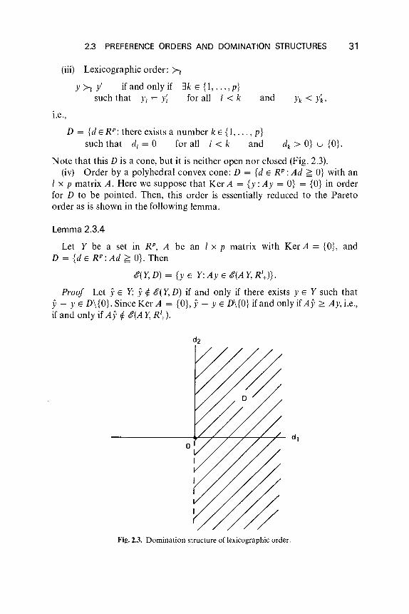
(iii) Lexicographic order: >-,r >. y' if and only if 3k E {I, ... , p}
such that Yi = Y; for all i < k
i.e.,
and Yk < y~,
D = {d E W: there exists a number k E {I, ... , p}such that d, = 0 for all i < k and dk > O} u {O}.
Note that this D is a cone, but it is neither open nor closed (Fig. 2.3).(iv) Order by a polyhedral convex cone: D = {d E W: Ad ~ O} with an
I x p matrix A. Here we suppose that Ker A = {y: Ay = O} = {O} in orderfor D to be pointed. Then, this order is essentially reduced to the Paretoorder as is shown in the following lemma.
Lemma 2.3.4
Let Y be a set in W, A be an I x p matrix with Ker A = {O}, andD = {d E W:Ad ~ O}. Then
I&"(Y, D) = {y E Y: Ay E I&"(A Y, R1+)}.
Proof Let y E Y; Yt$ 1&"( Y, D) if and only if there exists y E Y such thaty - y E D\{O}. Since Ker A = {O}, Y- Y E D\{O} if and only if Ay ~ Ay, i.e.,if and only if Ay t$ I&"(A Y, R1+).
Fig. 2.3. Domination structure of lexicographic order.
3 SOLUTION CONCEPTS AND SOMEPROPERTIES OF SOLUTIONS
In this chapter we discuss solution concepts for muItiobjective optimi-zation problems and investigate some fundamental properties of solutions.First, efficiency and proper efficiencyare introduced as solution concepts. Inthe second section, existence and external stability of efficient solutions arediscussed. The third section is devoted to conditions for the connectedness ofefficient sets. Three kinds of characterization for efficient or properly efficientsolutions-scalarization, best approximations, and constraint problems-are given in the fourth section. The final section deals with the Kuhn-Tuckerconditions for multiobjective problems.
3.1 Solution Concepts
As we have already mentioned, the concept of optimal solutions tomultiobjective optimization problems is not trivial and in itself debatable. Itis closely related to the preference attitudes of the decision makers. The mostfundamental solution concept is that of efficient solutions (also callednondominated solutions or noninferior solutions) with respect to the domi-nation structure of the decision maker, which is discussed in the firstsubsection. We also discuss another slightly restricted concept-properefficiency-in the second subsection.
3.1.1 EfficientSolutions
In this section we consider the muItiobjective optimization problem
(P) minimize f(x) = (fl(X),f2(X), ... ,fp(x) subject to x E X C W.
32
Let
3.1 SOLUTION CONCEPTS
Y = f(X) = {y: y = f(x), X E X}.
33
A domination structure representing a preference attitute of the decisionmaker is supposed to be given as a point-to-set map D from Y into RP.Though it might be natural to suppose that D(y) => R~ since a smaller valueis preferred for each}; (i = 1, ... , p), we do not assume this in order to dealwith more general multiobjective problems.
Definition 3.1.1 (Efficient Solution)
A point x E X is said to be an efficient solution to the multiobjectiveoptimization problem (P) with respect to the domination structure D iff(x) E 0"(Y, D); that is, if there is no x E X such thatf(x) E f(x) + D(f(x)) andf(x) # f(x) (i.e., such thatf(x) E f(x) + D(f(x))\{O}).
The following proposition is immediate.
Proposition 3.1.1
Given two domination structures D1 and Dz, D1 is said to be included byo, if
for all y E Y.
In this case,
Many interesting cases of efficient solutions are obtained when D is aconstant point-to-set map whose value is a constant (convex) cone. In suchcases, we identify the map (domination structure) with the cone D. Thenx E X is an efficient solution to the problem (P) if and only if there is nox E X such that f(x) - f(x) E D\{O}; namely, x is efficient if and only ifU(X) - f(x» (\ (-D) = {O}. If D is an open cone, it does not contain O.However, we consider D(y) = D u {O} and call D itself the dominationstructure in this book. As a matter offact it does not matter so much whetherD contains 0 or not since the set D\ {O} is used for the definition of efficientsolutions.
Remark 3.1.1
Given a closed convex cone D, some authors call x a weakly efficientsolution to the problem (P) if f(x) E 0"( Y, int D), i.e., if (f(X) - f(x)) (\(-int D) = 0 (Nieuwenhuis [N15, N16], and Corley [C15]). Weakly
34 3 SOLUTION CONCEPTS AND SOME PROPERTIES OF SOLUTIONS
efficient solutions are often useful, since they are completely characterizedby scalarization (see Corollary 3.4.1 later).
The following propositions are often very useful.
Proposition 3.1.2
Let D be a nonempty cone containing 0, then
S(Y,D) =:J S(Y+ D,D)
with equality holding if D is pointed and convex.
Proof The result is trivial if Y is empty, so we assume otherwise. Firstsuppose y E S(Y + D, D) but Y ¢ S(Y, D). If y ¢ Y, there exist y' E Y andnonzero dE D such that y = y' + d. Since OED, Y c Y+ D. Hence,y ¢ S(Y + D, D), which is a contradiction. If y E Y, we directly have a similarcontradiction.
Next suppose that D is pointed and convex, y E S(Y, D) buty ¢ S(Y + D, D). Then there exists a y' E Y+ D with y - y' = d' E D\{O}.Then y' = y" + d" with y" E Y, d" ED. Hence, y = y" + (d' + d") andd' + d" E D, since D is a convex cone. Since D is pointed, d' + d" #-°and soy ¢ S(Y, D), which leads to a contradiction. This completes the proof of theproposition.
Remark 3.1.2
It is clear that the pointedness of D cannot be eliminated in the inclusion
S(Y, D) c S(Y + D, D).
The convexity of D is also essential. In fact, let
and
which is pointed but not convex. Then (1, 1) E S(Y, D). However,
(1,1) = (0,0) + (t,O) + (t, 1) E Y+ D + D.
Hence (1, 1) ¢ S(Y + D, D) (see Fig. 3.1).

3.1 SOLUTION CONCEPTS 35
o 1 1"2
y
o--¥---..L.---Vl
Fig. 3.1. B(Y. D) ¢ 6'( Y + D, D). (Remark 3.1.2.)
Proposition 3.1 .3
Let Y1 and Y2 be two sets in RP, and let D be a constant dominationstructure on RP (a constant cone, for example). Then
1&"(Y1 + Y2,D) C 1&"(Y1, D) + 1&"(Y2,D).
Proof Let y E 1&"(Yl + Y2, D). Then y = yl + y2 for some yl E Y1 andy2 E Y2. We show that yl E 1&"(Y1, D). If we suppose the contrary, then thereexist y E Y1 and nonzero dE D such that yl = Y + d. Then y = yl + y2 =
Y + y2 + d and y + l E Y1 + Y2, which contradicts the assumptiony E 1&"(Y1 + Y2, D). Similarly we can prove that y2 E 1&"(Y2,D). Therefore,YE &(Y1, D) + &(Y2 , D).
Remark 3.1 .3
The converse inclusion of Proposition 3.1.3 does not always hold. Forexample, let
Y1 = Y2 = {(Yl'Y2):(Yl)2 + (Y2)2 ~ I} C R2
and D = R~. Then
and y2 = (0, -1) E 1&"(Y2,D).
However,
yl + y2 = (-1, -1) > (-)2, -)2)
= (- )2/2, - )2/2) + (- )2/2, - )2/2) E Y1 + Y2 •
Proposition 3.1.4
Let Y be a set in RP, D be a cone in RP, and a be a positive real number.Then
1&"(a Y, D) = a1&"( Y, D).
36 3 SOLUTION CONCEPTS AND SOME PROPERTIES OF SOLUTIONS
Proof The proof of this proposition is easy and therefore left to thereader.
The most fundamental kind of efficient solution is obtained when D is thenonnegative orthant R':- = {y E RP : y ~ O} and is usually called a Paretooptimal solution or noninferior solution.
Definition 3.1.2 (Pareto Optimal Solution)
A point xE X is said to be a Pareto optimal solution (or noninferiorsolution (Zadeh [Zl])) to the problem (P) if there is no x E X such thatf(x) s f(X).
A number of theoretical papers concerning muitiobjective optimizationare related to the Pareto optimal solution. In some cases a slightly weakersolution concept than Pareto optimality is often used. It is called weakPareto optimality, which corresponds to the case in which the dominationcone D\{O} is equal to the positive orthant R':- = {y E RP: y > O}.
Definition 3.1.3 (Weak Pareto Optimal Solutionv'
A point xE X is said to be a weak Pareto optimal solution to the problem(P) if there is no x E X such that f(x) < f(x).
3.1.2 Properly Efficient Solutions
This subsection is devoted to another slightly strengthened solutionconcept, proper efficiency. As can be understood from the definitions(particularly from Geoffrion's definition), proper efficiency eliminates un-bounded trade-offs between the objectives. It was originally introduced byKuhn and Tucker [KIO], and later followed by Klinger [K7], Geoffrion[G5], Tamura and Arai [T3] , and White [W9] for usual vector optimizationproblems with the domination cone R':-. Borwein [BI6, BI7], Benson [B7,B9], and Henig [H7] dealt with more general closed convex cones as thedomination cone. Hence, in this subsection, the domination cone D isassumed to be a nontrivial closed convex cone in RP unless otherwise noted(Definition 3.1.8 later).
Definition 3.1.4 (Tangent Cone)
Let S c RP and yES. The tangent cone to S at y, denoted by T(S, y), is theset of limits of the form h = lim tiY' - y), where {tk } is a sequence ofnonnegative real numbers and {I} is a sequence in S with limit y.
t cf. Remark 3.1.1.
3.1 SOLUTION CONCEPTS
Remark 3.1 .4
The tangent cone T(S, y) is always a closed cone.
37
Definition 3.1.5 (Borwein's Proper Efficiency)t
A point xE X is said to be a properly efficient solution of the multi-objective optimization problem (P) if
T(Y + D,f(x» n (-D) = {O}.
Proposition 3.1.5
If a point xE X is a properly efficient solution of (P) by the definition ofBorwein, then it is also an efficient solution of (P).
Proof If x is not efficient, there exists a nonzero vector d E D such thatd = f(x) - y for some y E Y. Let dk = (1 - l/k)d E D and t, = k fork = 1,2, .... Then
y + dk = f(x) - d + (1 - l/k)d = f(x) - (l/k)d ~ f(x) as k ~ 00,
and
tk(y + dk- f(x» = k(-d + (1 - l/k)d) = -d ~-d as k ~ 00.
Hence, T(Y + D,f(x» n (...I'D) =F {O}, and x is not properly efficient in thesense of Borwein.
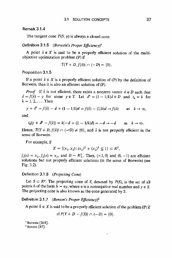
For example, if
X = {(Xl' x 2 ) : (XI)2 + (X 2)2 ~ I} C R 2,
fl(X) = xl,fl(X) = Xl' and D = R~. Then, (-1,0) and (0, -1) are efficientsolutions but not properly efficient solutions (in the sense of Borwein) (seeFig. 3.2).
Definition 3.1.6 (Projecting Cone)
Let S c RP. The projecting cone of S, denoted by P(S), is the set of allpoints h of the form h = Cty, where o: is a nonnegative real number and yES.The projecting cone is also known as the cone generated by S.
Definition 3.1.7 (Benson's Proper Efficiency)t
A point xE X is said to be a properly efficient solution of the problem (P) if
cl P(Y + D - f(x» n (-D) = {O}.
t Borwein [B16].I Benson [B7].

38 3 SOLUTION CONCEPTS AND SOME PROPERTIES OF SOLUTIONS
---......----+-----+---- X 1 = Y1-1
-1
Fig. 3.2. Efficient but not properly efficient solutions.
Since T(Y + D, f(x» c cl P(Y + D - f(x» Benson's proper efficiencystrengthens Borwein's proper efficiency. The converse, however, does notalways hold (see Example 3.1.1 later).
Lemma 3.1.1
Let S be a convex set and yES. Then
T(S, y) = cl P(S - y),
which is a closed convex cone.
Proof It is obvious that cl P(S - y) is a closed convex cone. So it sufficesto show that cl P(S - y) c T(S, y), since the converse follows directly fromthe definitions. Since T(S, y) is closed, we need only to prove thatP(S - y) c T(S, y). Let h E P(S - y). Then h = f3(y' - y) for some 13 ~ 0 andy' E S. Let
l = [1 - (l/k)]y + (l/k)y'
and tk = 13k ~ O. Then tk(l - y) = f3(y' - y). Hence l E S from the con-vexity of S, and
l--> y as k --> 00.
Thus h E T(S, y), and the proof is completed.

3.1 SOLUTION CONCEPTS 39
Theorem 3.1.1
If xis a properly efficient solution of the problem (P) in the sense ofBenson, it is also a properly efficient solution of (P) in the sense of Borwein. IfX is a convex set and iff is a D-convex function on X (see Definition 2.1.15),then the converse also holds; that is, Borwein's proper efficiency is equivalentto Benson's proper efficiency.
Proof If D is a con vex cone and f is D-con vex on the con vex set X, the setY+ D is a convex set (Proposition 2.1.21). Hence, cl PlY + D - f(x)) =T(Y + D,f(x)) by Lemma 3.1.1. Therefore, the proper efficiency in the senseof Borwein is equivalent to that in the sense of Benson.
The following definition of proper efficiency by Henig does not require thedomination cone D to be closed.
Definition 3.1.8 (Henig's Proper Efficiency)t
(i) A point xE X is said to be a global properly efficient solution of (P) if
f(x) E g( Y, D'),
for some convex cone D' with D\{O} c int D'.(ii) A point xE X is a local properly efficient solution of (P) if, for every
s > 0, there exists a convex cone D' with D\{O} c int D', such that
f(x) E g(( Y + D) r. (f(x) + eB), D'),
where B is the closed unit ball in RP.
These definitions are essentially the same as Benson's and Borwein's,respectively.
Theorem 3.1.2
If D is closed and acute, then Henig's global (respectively, local) properefficiency is equivalent to Benson's (respectively, Borwein's) proper efficiency.
Theorem 3.1.3
Any global properly efficient solution is also locally properly efficient.Conversely, if D is closed and acute, and if
y+ r. (-D) = {O},
t Henig [H7].

40 3 SOLUTION CONCEPTS AND SOME PROPERTIES OF SOLUTIONS
then local proper efficiency is equivalent to global proper efficiency. Here y+is an extension of the recession cone of Yand is defined by
y+ = {y': there exist sequences {lXd c R, {l} c Ysuch that IXk > 0, IXk -> °and IXk l -> y'}.
(The condition y+ n (- D) = {a} will later be called the D-boundedness ofY. See Definition 3.2.4.)
The proofs of the above two theorems are rather long, and so they areomitted here. The reader may refer to Henig [H7].
When D = R~, Geoffrion's definition of properly efficient solutions is wellknown.
Definition 3.1.9 (Geoffrion's Proper Efficiency)t
When D = R~, a point xis said to be a properly efficientsolution of(P) ifitis efficient and if there is some real M > °such that for each i and each x E Xsatisfyingji(x) < /;(x), there exists at least one j such that .fj(x) < .fj(x) and
(h(x) - h(x))/(.fj(x) - .fj(x)) ~ M.
Theorem 3.1.4
When D = R~, Geoffrion's proper efficiency is equivalent to Benson'sproper efficiency, and therefore is stronger than Borwein's proper efficiency.
Proof Geoffrion => Benson: Suppose that xis efficientbut not properlyefficient in the sense of Benson, namely, that there exists a nonzero vectordE cl P(Y + R~ - f(x)) n (-R~). Without loss of generality, we mayassume that d1 < -I, d, ~ °(i = 2, ... , p). Let
tk(f(Xk) + rk
- f(x)) -> d,
where rk E R~, t k > 0, and x k E X. By choosing a subsequence we canassume that
I = {i :h(xk) > h(x)}
is constant for all k (and nonempty since x is efficient). Take a positivenumber M. Then there exists some number ko such that for k ~ ko
fl(X k) - fl(X) < -1/2tk
and
h(~) - h(x) ~ 1/2Mtk (i = 2, ... , p).
"Geoffrion [G5].

3.1 SOLUTION CONCEPTS
Then for all i E 1, we have (for k ~ ko)
o< J;(xk) - J;(x) ~ 1/2Mtk
and for k ~ ko,
41
f1(X) - f1(Xk) 1/2tk _ M
J;(xk) - J;(x) > 1/2Mtk - .
Thus xis not properly efficient in the sense of Geoffrion.
Benson => Geoffrion: Suppose that xis efficient but not properly effi-cient in the sense of Geoffrion. Let {Mk } be an unbounded sequence ofpositive real numbers. Then, by reordering the objective functions, ifnecessary, we can assume that for each M; there exists an x k E X such thatfl(Xk) <f1(X) and
(f1(x) - f1 (Xk))/(J;(~) - J;(x)) > M,
for all i = 2, ... , p such that J;(xk) > J;(x). By choosing a subsequence of{Mk } , if necessary, we can assume that
1 = {i :J;(xk) > J;(x)}
is constant for all k (and nonempty since xis efficient). For each k let
tk = (f1(X) - f1(Xk))-1.
Then tk is positive for all k. Let
r7 = {~(X) - J;(xk)
Clearly rk E R~, and
for i = 1 or i E 1,for i i= 1, i ¢ 1.
Let
d, = lim tk[J;(Xk) + r~ - J;(x)J.k-oo
Clearly d1 = -1 and d, = 0 when i i= 1 and i ¢ 1. Since {Mk } is anunbounded sequence of positive real numbers, we have
Thus,
d, = 0 for i E 1.
d = (-1,0, ... ,0) i= 0 E cl P(f(X) + R~ - f(x)) n (- R~).

42 3 SOLUTION CONCEPTS AND SOME PROPERTIES OF SOLUTIONS
Hence x is not a properly efficient solution of (P) in the sense of Benson, aswas to be proved.
Paying attention to multiobjective programming problems, we mayconsider another type of proper efficiency that was defined earlier than thepreceding ones.
A multiobjective programming problem is defined as
(P')minimize f(x) = (fl(X), ... ,fix»
subject to x E X = {x: g(x) = (gl(X), ... , gm(X» ~ OJ.
That is, X is supposed to be specified by m inequality constraints. Here, allthe functions}; and gj are assumed to be continuously differentiable.
Definition 3.1.10 (Kuhn- Tucker's Proper Ejficiency)t
A point xis said to be a properly efficient solution of the problem (Pi) if it isefficient and if there is no h such that
and
<V};(x), h) ~ 0
<V};(Xi, h) < 0
for any i = 1, ... , p.
for some i,
<Vgj(x), h) ~ 0 for any j E J(x) = {j: g/x) = OJ.
Theorem 3.1 .5
Suppose that the functions}; and gj (i = 1, ... , p, j = 1, ... , m) are convex.Ifxis a properly efficient solution of (Pi) in the sense of Kuhn-Tucker, then itis also properly efficient in the sense of Geoffrion.
Proof This theorem can be established as a corollary of Theorems 3.5.1and 3.5.2, which will be given later.
Definition 3.1.11 (Kuhn-Tucker Constraint Qualification)
Problem (Pi) is said to satisfy the Kuhn-Tucker constraint qualification atxE X if, for any hEW such that <Vgj(x),h) ~ 0 and for any j E J(x) :={j: gix) = OJ, there exist i » 0, a vector-valued function (J on [0, t]differentiable at t = 0, and a real number o: > 0, such that
8(0) = x, g(8(t») ~ 0 for any t E [0, i], 8(0) = oh.
t Kuhn and Tucker [KIO].

3.1 SOLUTION CONCEPTS 43
for j E J(x).
for i = 2, ... , p,
-(Vfl(X),rxh) + o(tk)!tk(V;;(x), rxh) + o(tk)!tk
Theorem 3.1 .6
Suppose that (P') satisfies the Kuhn-Tucker constraint qualification at X.Ifxis a properly efficient solution of (P') in the sense of Geoffrion, then it isalso properly efficient in the sense of Kuhn-Tucker.
Proof Suppose that xis efficient but not properly efficient in the sense ofKuhn-Tucker. Then there exists an h E R" such that
(Vil (x), h) < 0,
(V/;(x), h) ~ 0
(Vgj(x), h) ~ 0
(Reorder the objective functions, if necessary.) From the Kuhn-Tuckerconstraint qualification, there exists a continuously differentiable arc 8(t)(0 ~ t ~ t) such that 8(0) = x, g(8(t» ~ 0, and ~(O) = ah, Consider asequence of positive numbers {td ~ O. By taking a subsequence, if necessary,we may assume that
1 = {i :h(8(tk» > h(x)}
is constant. Since, for i E 1,h((J(tk» - ;;(i) = tk(V;;(x), rxh) + o(tk) > 0
and(V;;(x), h) ~ 0,
we have
(Vh(x), rxh) = 0,
Then, since (Vfl(X), h) < 0,
fl(X) - fl((J(tk»h(8(tk» - h(X)
diverges to + 00 as k ~ 00. This implies that x is not properly efficient in thesense of Geoffrion. This completes the proof of the theorem.
Relationships among some different proper efficiency concepts aredepicted in Fig. 3.3. Some examples are given in the following.
Example 3.1.1 [Borwein, but not Benson (= Geoffrion) - Fig. 3.4]t
Let
X = {(Xl,X2) E R 2: Xl + X2 ~ O} U {(XI,X2) E R~ :XI ~ I}
U {(Xl' X 2) E R 2: X2 ~ I},
j~(Xl,X2) = Xl' f2(X I,X2) = X 2,
D = R~.
t Benson [B7].
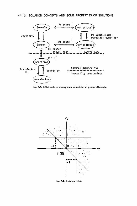
44 3 SOLUTION CONCEPTS AND SOME PROPERTIES OF SOLUTIONS
11' 11 0: acute, closedII ~ recession condition
Kuhn-Tucker 11ft'.tCQ "J. 1/ convexi y
general constraints==========================
inequality constraints
Fig. 3.3. Relationships among some definitions of proper efficiency.
Y2
, ..
----..L--~t--_+---- Y1
Fig. 3.4. Example 3.1.1.

o
.... x: .
. ' ' . .. . ,\ ..AX
3.1 SOLUTION CONCEPTS
Y2
o
-2
Fig. 3.5. Example 3.1.2.
45
:-,r--=--- Yl
Then x= (0,0) is a properly efficient solution according to Borwein'sdefinition. However, it is not properly efficient in the sense of Geoffrion or ofBenson. Note that X is not convex and that Y is not R~ -bounded.
Example 3.1.2 [Geoffrion, but not Kuhn-Tucker-Fig. 3.5]t
Let,
X = {(Xl' X2) E R2: -Xl ~ 0, -X2 ~ 0, (Xl - I? + X2 ~ O},
fl(X) = - 3xI - 2x2 + 3, f2(x) = -Xl - 3x 2 + 1,
D = R~.
Then x= (1,0) (at which the Kuhn-Tucker constraint qualification is notsatisfied) is not a Kuhn-Tucker properly efficient solution, although it isproperly efficient by Geoffrion's definition.
Example3.1.3 [Kuhn-Tucker, but not Geoffrion-Fig. 3.6]t
Let
X = {x E R : X ~ O},
fl(x) = _x2 be not convex,
D = R~.
Then x= 0 is properly efficient in the sense of Kuhn-Tucker but not ofGeoffrion.
Any properly efficient solution is, in general, an efficient solution, but notvice versa. (We will later prove that every efficient point is contained in the
f Tamura and Arai [T3].
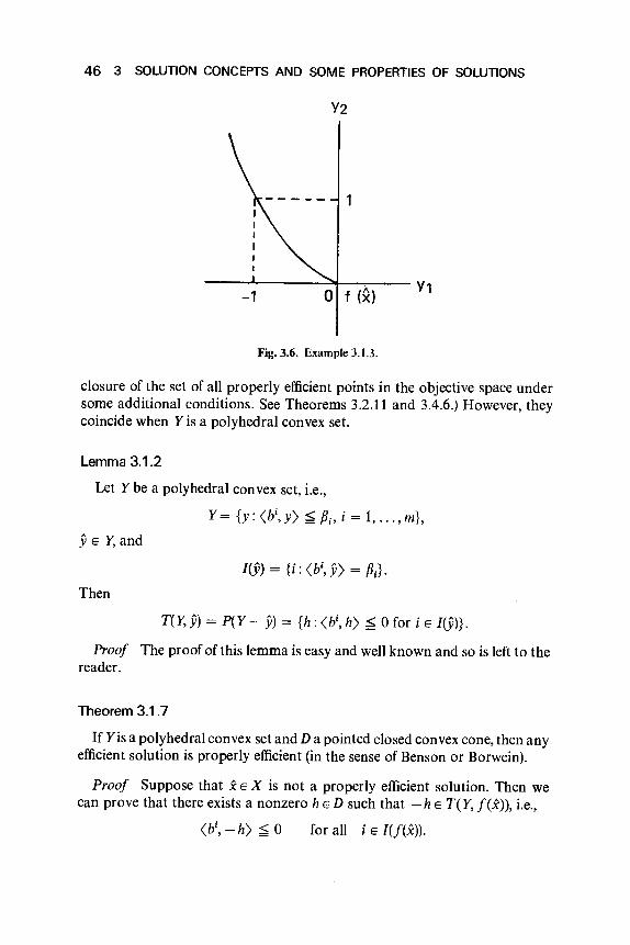
46 3 SOLUTION CONCEPTS AND SOME PROPERTIES OF SOLUTIONS
Y2
Fig. 3.6. Example 3.1.3.
closure of the set of all properly efficient points in the objective space undersome additional conditions. See Theorems 3.2.11 and 3.4.6.) However, theycoincide when Y is a polyhedral convex set.
Lemma 3.1.2
Let Y be a polyhedral convex set, i.e.,
Y= {y: <bi,y) ~ Pi' i = 1, ... ,m},
YE Y, and
Then
T(Y, y) = P(Y - y) = {h: <bi, h) ~ 0 for i E I(Y)}.
Proof The proof of this lemma is easy and well known and so is left to thereader.
Theorem 3.1 .7
If Yis a polyhedral convex set and D a pointed closed convex cone, then anyefficient solution is properly efficient (in the sense of Benson or Borwein).
Proof Suppose that ~ E X is not a properly efficient solution. Then wecan prove that there exists a nonzero h e D such that - hE T(Y, f(~», i.e.,
for all i E I(f(x».
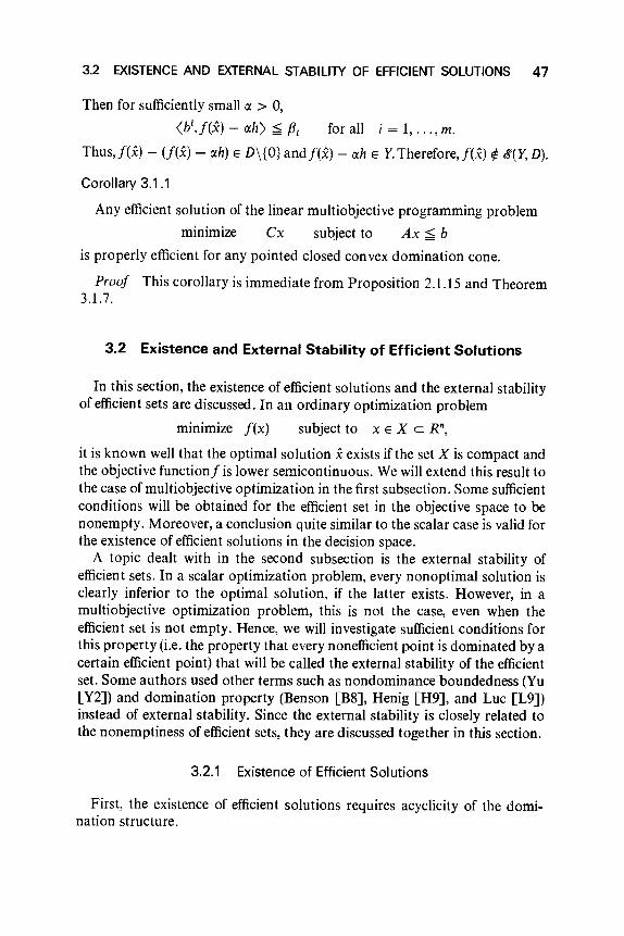
3.2 EXISTENCE AND EXTERNAL STABILITY OF EFFICIENT SOLUTIONS 47
Then for sufficiently small « > 0,
<bi,f(x) - rxh) ~ Pi for all i = 1, ... , m.
Thus.j'(x) - (f(x) - tl.h) E D\{O} andf(x) - rxh E Y. Therefore.j'(x) rt l3"(Y, D).
Corollary 3.1 .1
Any efficient solution of the linear multiobjective programming problem
minimize ex subject to Ax ~ b
is properly efficient for any pointed closed convex domination cone.
Proof This corollary is immediate from Proposition 2.1.15 and Theorem3.1.7.
3.2 Existence and External Stability of Efficient Solutions
In this section, the existence of efficient solutions and the external stabilityof efficient sets are discussed. In an ordinary optimization problem
minimize f(x) subject to x E X eRn,
it is known well that the optimal solution xexists if the set X is compact andthe objective functionf is lower semicontinuous. We will extend this result tothe case of multiobjective optimization in the first subsection. Some sufficientconditions will be obtained for the efficient set in the objective space to benonempty. Moreover, a conclusion quite similar to the scalar case is valid forthe existence of efficient solutions in the decision space.
A topic dealt with in the second subsection is the external stability ofefficient sets. In a scalar optimization problem, every nonoptimal solution isclearly inferior to the optimal solution, if the latter exists. However, in amultiobjective optimization problem, this is not the case, even when theefficient set is not empty. Hence, we will investigate sufficient conditions forthis property (Le. the property that every nonefficient point is dominated by acertain efficient point) that will be called the external stability of the efficientset. Some authors used other terms such as nondominance boundedness (Yu[Y2]) and domination property (Benson [B8], Henig [H9], and Luc [L9])instead of external stability. Since the external stability is closely related tothe nonemptiness of efficient sets, they are discussed together in this section.
3.2.1 Existence of Efficient Solutions
First, the existence of efficient solutions requires acyclicity of the domi-nation structure.

48 3 SOLUTION CONCEPTS AND SOME PROPERTIES OF SOLUTIONS
Definition 3.2.1 (Acyclicity)
A domination structure D is said to be acyclic if it has no cycle; in otherwords, if for all n = 1,2, ... , it never occurs that
yl E y2 + D(yZ)\{O}, y2 E y3 + D(y3)\{O}, ... , Y' E yl + D(yl)\{O}
(i.e., yl -< y2 -< ... <; yn -< yl).
Remark 3.2.1
If a domination structure D is acyclic, it is also asymmetric. Conversely,every transitive and asymmetric domination structure is acyclic.
The following theorem is the existence result with a general dominationstructure; namely, D is not assumed to be a constant cone.
Theorem 3.2.1 t
If a domination structure D on Yis acyclic, the sets D(y)\{OJ are open andYis non empty and compact, then
t!(Y, D) i= 0.
Proof If we suppose, to the contrary, that
t!(Y, D) = 0.
then for any y E Ythere exists y' E Ysuch that y E y' + D(y')\ {O}. Thus
Yc U(y + D(y)\{O}).yeY
Thus, the family of the sets {y + D(y)\{O}} forms an open cover of Y. Since Yis compact, there is a finite subcover {l + D(l)\{O}} (i = 1, ... , n). Then, forany i E {1, ... ,n},
lEi + D(yi)\{O} for some j E {1, ... , n}.
However, this contradicts the assumption that D is acyclic. Hence,
t!(Y,D) i= 0·
The following example shows that the condition of openness of D(y)\{OJcannot be eliminated in the above theorem.
t Hazen and Morin [H6].
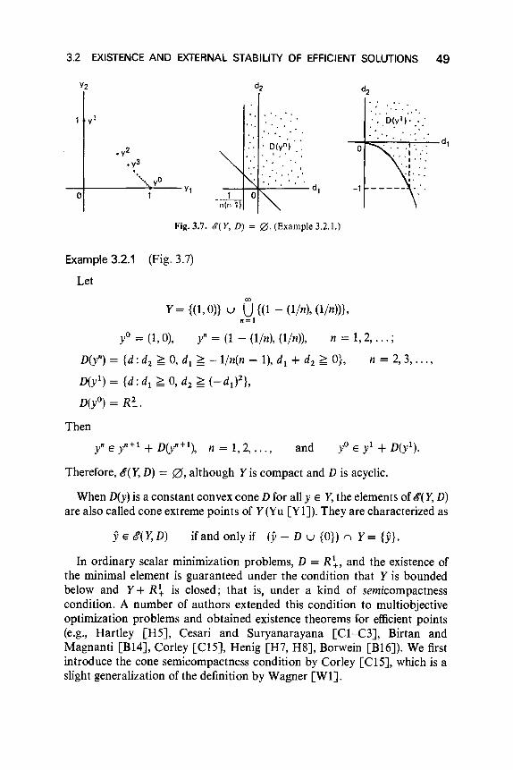
3.2 EXISTENCE AND EXTERNAL STABILITY OF EFFICIENT SOLUTIONS 49
1 yl
o
• y2
• y3.•••••• yO
1
' .. '. -
.' . D(y") ..••• I.'
Fig. 3.7. 6'(Y, D) = 0. (Example 3.2.1.)
Example 3.2.1 (Fig. 3.7)
Letoo
Y = {(I,O)} u U{(I - (lin), (lin))),"=1
yO = (1,0), y" = (1 - (lin), (lin)), n = 1,2, ... ;
D(y") = {d:dz ~ 0, d, ~ -lln(n -I), d1 + dz ~ O}, n = 2,3, ... ,
D(y1) = {d: d1 ~ 0, dz ~ (-d1? },
D(yO) = Rt.Then
y" E y"+ 1 + D(y" + 1), n = I, 2, ... , and
Therefore, 6"(Y, D) = 0, although Yis compact and D is acyclic.
When D(y) is a constant convex cone D for all y E Y, the elements of 6"(Y, D)are also called cone extreme points of Y(Yu [YI]). They are characterized as
yE g(Y, D) if and only if (y - D u {O}) n Y= {y}.
In ordinary scalar minimization problems, D = R~, and the existence ofthe minimal element is guaranteed under the condition that Y is boundedbelow and Y+ R~ is closed; that is, under a kind of semicompactnesscondition. A number of authors extended this condition to multiobjectiveoptimization problems and obtained existence theorems for efficient points(e.g., Hartley [H5], Cesari and Suryanarayana [CI-C3], Birtan andMagnanti [BI4], Corley [CI5], Henig [H7, H8], Borwein [BI6]). We firstintroduce the cone semicompactness condition by Corley [CI5], which is aslight generalization of the definition by Wagner [WI].
50 3 SOLUTION CONCEPTS AND SOME PROPERTIES OF SOLUTIONS
Definition 3.2.2 (Cone Semicompactness)
Let D be a cone and Y be a set in RP. Y is said to be D-semicompact ifeveryopen cover of Yof the form {(y1 - cl D)C : y1 E Y, Y E I'} has a finite subcover.Here r is some index set and the superscript c denotes the complement of aset.
Theorem 3.2.2
IfD is an acute convex cone and Y is a nonempty D-semicompact set in RP,then $(Y, D) -# 0.
Proof In view of Proposition 3.1.1,
$(Y, cl D) c $(Y, D).
Hence, it suffices to prove the case in which D is a pointed closed convexcone. In this case, D defines a partial order ~D on Yas
i ~D y2 if and only if y2 - yl ED.
An element in $(Y, D) is a minimal element of Y with respect to ~D'
Therefore, we will show that Y is inductively ordered and apply Zorn'slemma to establish the existence of minimal elements. Suppose to thecontrary that Y is not inductively ordered. Then, there exists a totallyordered set Y = {y1: y E I'} in Ywhich has no lower bound in Y. Thus,
n[(y1 - D) n y] = 0,1Er
otherwise any element of this intersection is a lower bound of Y in Y. It nowfollows that for any y E Y, there exists y1 E Y such that y ¢ y1 - D. Sincey1 - D is closed, the family {(y1 - D)C : y E T} forms an open cover of Y.Moreover, y1 - D C y1' - D if and only if y1 ~D y1', and so they are totallyordered by inclusion. Since Y is D-semicompact, the cover has a finitesubcover, and hence there exists a single yY E Y such that
Yc (yY - D)c.
However, this contradicts the fact yY E Y. Therefore, Y is inductively orderedby ~D and $(Y, D) -# 0 by Zorn's lemma.
It may be troublesome to check the cone semicompactness condition.Hartley [H5] used the slightly stronger cone compactness condition.
Definition 3.2.3 (Cone Compactness)
Let D be a cone in RP. A set Y c RP is said to be D-compact if, for anyy E Y, the set (y - cl D) n Y is compact.
3.2 EXISTENCE AND EXTERNAL STABILITY OF EFFICIENT SOLUTIONS 51
Proposition 3.2.1
If Y is D-compact, then Y is D-semicompact.
Proof Let a family of sets
{(yY - cl D)C : yY E Y, Y E I'}
be an open cover of Y. For an arbitrary lEY, the subfamily
{(yY - cl D)C : yY E Y, y E T, y =f. y}
forms an open cover of (yY - cl D) n Y. Since from the definition of D-compactness, (l - cl D) n Y is compact, this subfamily has a finite sub-cover, which together with (yY - cl D)C constitutes a finite subcover of Y. Theproof is completed.
Remark 3.2.2
A compact set is D-compact and so D-semicompact. However, a D-compact set is not necessarily compact. For example, take D = R~ andY = {y E R2
: Yt + Y2 ~ O} (Hartley [H5]).
Theorem 3.2.3
Let D be an acute convex cone in RP. If Y c RP is nonempty and D-compact, then tS'(Y,D) =f. 0·
Proof This result is immediate from Theorem 3.2.2 and Proposition3.2.1. although the direct proof can be seen in Hartley [H5].
Some authors used conditions in terms of recession cones of feasible sets(Bitran and Magnanti [B14], Henig [H7]). Here we adopt an extendeddefinition of the recession cone by Henig, since Y is not necessarily convex.As in Theorem 3.1.3, for Y::J RP, its extended recession cone y+ is defined by
y+ = {y': there exist sequences {CXk} c Rand {I} c Ysuch that CXk > 0, CXk ~ 0, and cxk! -. y'}.
Remark 3.2.3
It is clear that y+ is a closed cone and that O+y c Y+. On the other hand,O+Yis not necessarily closed even if Yis convex (Rockafellar [R7], p. 63).

52 3 SOLUTION CONCEPTS AND SOME PROPERTIES OF SOLUTIONS
Lemma 3.2.1 t
Let Ybe a nonempty set. Then
(i) Yis bounded if and only if y+ = {O},(ii) if Yis closed and con vex, y+ = 0+Y.
Lemma 3.2.2 t
Let {Y;} ieI be an arbitrary collection of nonempty closed sets. Then
(nY;)+ C nY/.ieI ieI
Lemma 3.2.3 §
Let Y1 and Y2 be nonempty closed sets in RP. If
Yt n (-yn = {O},
then Y1 + Y2 is a closed set.
Proof Let {Y~ + ;1} be a sequence such that Y~ E Y1 , and Y~ E Y2 andYt + >1-+ y. If {Yt} has no convergent subsequence, IIYtII-+ 00 as k -+ 00.
Hence (Yt + y~)/IIYt II -+ o. We may assume without loss of generalitythat Yt/IIYt II -+ Yl with IIYll1 = 1. Clearly Yl E Yt· Moreover Y~/IIYt II -+ - Yl'which is in Y2+ from the definition. Thus Yl E Yt n (- Yn, which con-tradicts the hypothesis. Hence, suppose that {Yt} converges to some 91' Then{>1} clearly converges to Y - Yl' Since Y1 and Y2 are closed, 91 E Y1,
Y - 91 E Y2 , and so y = 91 + (y - h) E Y1 + Y2 , as was to be proved.
Definition 3.2.4 (Cone Closedness and Cone Boundedness)
Let Ybe a nonempty set in RP, and Jet D be a cone in RP. Then Yis said tobe
(i) D-closed if Y+ cl D is closed, and(ii) D-bounded if y+ n (-cl D) = {O}.
Remark 3.2.4
Let D be a pointed cone. If there exists a point yO E RP such thatYc r" + cl D, then it is clear that Yis D-bounded. This hypothesis was usedas the definition of D-boundedness in Tanino and Sawaragi [TIl].
t Henig [H7].
I Henig [H7] cf. Proposition 2.1.9.I cf. Proposition 2.1.11.

3.2 EXISTENCE AND EXTERNAL STABILITY OF EFFICIENT SOLUTIONS 53
Lemma 3.2.4
Let D be a pointed, closed, convex cone and Y be a nonempty set in RP.Then, y+ n (-D) = {a} if and only if(Y + D)+ n (-D) = {a}.
Proof Since (Y + D)+ ::J Y+, it is clear that y+ n (-D) = {a} when(Y + D)+ n (-D) = {a}. To prove the only if part, suppose that(Y + D)+ n (-D) # {a}. Then there exist sequences {ad c Rand {y" + dk
}
such that !Xk > 0, CXk .... 0, y" E Y, dk E D, CXk(yk + dk) -+ -d # °E -D. Thereare two cases: (i) {cxkdk} has a convergent subsequence, and (ii) {akdk} has noconvergent subsequence.
Case (i) By taking a subsequence, if necessary, we may assume withoutloss of generality that akdk .... d', Since D is closed, d' E D. Therefore,(Xkyk -+ -d - d', which is a nonzero vector in y+ n (-D) since D is a pointedconvex cone. Hence, y+ n (-D) # {a}.
Case (ii) In this case, {(Xkdk} is unbounded, so {!Xkdk}+ # {a} fromLemma 3.2.1(i). Namely, we may assume by taking a subsequence of {cxkdk}that there exists another sequence {13k} such that
13k > 0, 13k .... 0, and Pk(!Xkdk) ....d # 0.
Since D is closed, dE D. Then
(Pk(Xk)y" ...... -d, with Pk(Xk > 0, Pk(Xk .... 0.
In fact,
II(Pk(Xk)y" + dll = IIPk«(Xk(y" + dk) + d) - (Pk(Xk dk - d) - Pkdll
~ Pkll!Xk(y" + dk) + dll + IIPk(Xk dk - dll + Pklldll
.... ° as k .... 00.
Thus, we have proved that y+ n (-D) # {O}.
Lemma 3.2.5
Let D be a convex cone and Ybe a set in RP. If Y + cl D is D-semicompact,then Y is also D-semicompact.
Proof Let {(y1 - cl D)C : y1 E Y, ')I E I'} be an open cover of Y. For anarbitrary y E Y, let y E (l - cl D)c with lEY. Since cl D is a convex cone.
(yi' _ cl D)C ::J Y + cl D.
In fact, if y + d E yi' - cl D for some d E cl D, y E yi' - cl D, which is acontradiction. Hence {(y1 - cl D)C : y1 E Y, ')I E I"} is also an open cover ofY + cl D. Since Y + c1 Dis D-semicompact, this cover has a finite subcover,which is, of course, a subcover of Y. Hence Y is D-semicompact.

54 3 SOLUTION CONCEPTS AND SOME PROPERTIES OF SOLUTIONS
Proposition 3.2.2
Let D be an acute convex cone in RP and Y be a nonempty set in RP. IfY is D-closed and D-bounded, then Y+ cl D is D-compact, and Y is D-semicompact.
Proof Let Y E Y+ cl D. Since Y - cl D and Y+ cl D are both nonemptyclosed sets, (y - cl D) n (Y+ cl D) is closed. Therefore, from Lemmas 3.2.2and 3.2.4
((y - cl D) n (Y+ cl D))+ c (y - cl D)+ n (Y+ cl D)+
= (-clD) n (Y+ clD)+
= {O}
since Y is D-bounded. Thus, in view of Lemma 3.2.1 (i), (y - cl D) n(Y+ cl D) is bounded. Therefore, Y+ cl Dis D-compact, and so Y+ cl DisD-semicompact from Proposition 3.2.1. Hence, from Lemma 3.2.5, Y is D-semicompact.
Theorem 3.2.4
Let D be an acute convex cone in RP and Ybe a nonempty, D-closed, D-bounded set in RP. Then C(Y,D):I= 0.
Proof This theorem can be proved easily by Theorem 3.2.2 andProposition 3.2.2.
We now give some examples of D-semicompact sets with D = R~.
Example 3.2.2
(i) (Fig. 3.8) Let
Y= {(Yl' Y2): (Yl)2 + (Y2)2 ~ 1, Yl < 0, Yl < O}.
Then Yis R~-compact, R~- bounded, but not R~-closed, and
C(Y,R~) = {(Yl'Y2):(Yl)2 + (Y2? = 1, Yl < 0, Yl < O}.
(ii) (Fig. 3.9) Let
Y= {(Yl,Yl):YlY2 = 1, Yl < O}.
Then Y is R~-compact, R~-closed, but not R~-bounded. In fact{(-I, 0), (0, -I)} c Y + n (-R~). In this case, C(Y, R~) = Y.
(iii) (Fig. 3.10) Let
Y= {(Yl' Yl): (Yl)2 + (Y2)2 < I}V {(Yl' Y2): (Yl)2 + (Y2f = 1, Yl ~ 0, Y2 ~ O}.
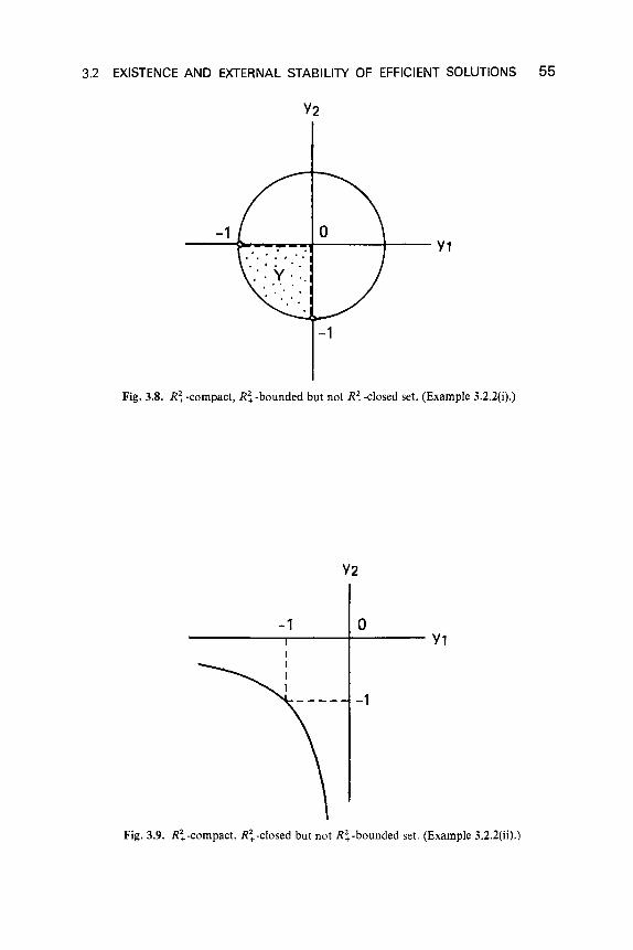
3.2 EXISTENCE AND EXTERNAL STABILITY OF EFFICIENT SOLUTIONS 55
Y2
-1---o__..-........---~-- Y1
-1
Fig. 3.8. Ri -compact, R~ -bounded but not R~ -closed set. (Example 3.2.2(i).)
Y2
-1 o-------r----+---- Y1
-1
Fig. 3.9. R~-compact, R~-closed but not R~-bounded set. (Example 3.2.2(ii).)

56 3 SOLUTION CONCEPTS AND SOME PROPERTIES OF SOLUTIONS
Y2
. .. .. .., .' I
: -. '. '.: './.' ", . I, . " '/. -. /
"
- -/,.,. 4 ..............
/ . '- . . ,I " . - '. '\
I . . . \-1 Y '.... \
-1
Fig. 3.10. R~-c1osed, R~·bounded but not R~-compact set. (Example 3.2.2(iii).)
Then Yis Rl-closed and R~-bounded, but not Rl-compact. In this case,
t9'(Y, Rl) = {(Yl' Yz): (Yl? + (yz)Z = 1, Yl ~ 0, Yz ~ O}.
As can be seen from these examples, the concepts introduced by thevarious authors are different, in general. However, they coincide in theconvex case, as shown by the following proposition.
Proposition 3.2.3
Let D be a pointed closed convex cone and Y be a nonempty, closedconvex set in RP. Then the following are equivalent:
(i) O+y n (-D) = {O};(ii) Yis D-closed and D- bounded;
(iii) Yis D-compact;(iv) (0+Y)°nD"°#0;(v) Yis D-semicompact.
Proof The equivalence of (i) and (iv) is immediate from Proposition 2.1.8.From Lemma 3.2.1(ii), condition (i) is equivalent to the D-boundedness of Y.In view of Proposition 2.1.11 or Lemma 3.2.3, Y+ D is closed if
o+Y n (-0+D) = o+Y n (-D) = {O},
Le., if Y is D-bounded. Thus we have proved the equivalence of (i) and (ii).The proof of (ii) ~ (iii) is essentially the same as the proof of Proposition

3.2 EXISTENCE AND EXTERNAL STABILITY OF EFFICIENT SOLUTIONS 57
3.2.2. Next, we prove (iii) = (i). Take any y E Y. Then (y - V) r, Y iscompact, and from Proposition 2.1.10,
O+«y - V) n Y) = {O}.
From Proposition 2.1.9, this implies that
O+y n (-V) = {O}.
Finally, (iii) =(v) (Proposition 3.2.1) or (ii) =(v) (Proposition 3.2.2),(v) = Iif( Y, V) ¥- 0, and we later prove that Iif( Y, V) ¥- 0 = (i) in Theorem3.2.5.
In the analysis of efficient sets, the V-compactness condition was used byHartley [H5] and Naccache [Nl], while Henig [H7] used a conditionsimilar to V-boundedness and V-closedness. Borwein [B16] and Bitran andMagnanti [B14] used conditions (i)or (iv)in the above proposition for closedconvex Y. Corley [C15] used the V-semicompactness condition. However, ascan be seen from the above propositions, they are closely related to oneanother.
Now we can prove that if Y is closed convex, V-compactness is alsonecessary for 1if(Y, V) to be nonempty. (Sufficiency has been already estab-lished in Theorem 3.2.2 or 3.2.3.)
Theorem 3.2.5
Let V be a pointed closed convex cone and Ybe a nonempty closed convexset. Then 1if(Y, V) ¥- 0 if and only if any of the conditions in Proposition3.2.3 is satisfied.
Proof We need only to prove that O+Yn (-V) = {O} if 1if(Y,V) ¥- 0.Suppose, to the contrary, that some nonzero - d belongs to the set0+ Y n (-V). Then, for each y E Y, Y - dEY and so y if; 1if(Y, V). Hence,1if(Y, V) = 0. This completes the proof of the theorem.
Remark 3.2.5
In Theorem 3.2.5, the condition that Y be closed and convex may bereplaced by the one that Y be V-closed and V-convex.
When Y is a polyhedral convex set, the existence condition of efficientsolutions (which are also properly efficient solutions by Theorem 3.1.7) canbe obtained as follows.
58 3 SOLUTION CONCEPTS AND SOME PROPERTIES OF SOLUTIONS
Theorem 3.2.6
Let Y be a nonempty, polyhedral convex set and D be a pointed, closedconvex cone in RP.Then c!(Y, D) is nonempty if and only if
(i) when Yis expressed as
Y= {y: (bi,y) ~ Pi' i = 1, . . . ,m},
there is no d i= 0 E D such that (b i, d) ~ 0 or, equivalently, the finitely
generated cone with the generators {b l, •.• , bin} and IYO have a common
nonzero vector.(ii) when Yis expressed as
y= {y:y = t (Xi a i, (Xi ~ 0 (i = 1, ... ,m), f (Xi = I},i=1 i=l
ai ¢ - D for any i = k + 1, ... , m.
Proof The results follow immediately from Theorem 3.2.5 andPropositions 2.1.8,2.1.13, and 2.1.14.
We conclude this subsection with an existence theorem of efficientsolutions in the decision space, which is a quite natural extension of thescalar case. For this purpose, we introduce an extended semicontinuityconcept of functions according to Corley [CIS].
Definition 3.2.5 (Cone Semicontinuity)
Let D be a cone in RP. A function f: W --+ RP is said to be D-semicontinuous if
f- 1(y - cl D) = {x E W: Y - f(x) E cl D}
is closed for each Y E RP.
Remark 3.2.6
If p = 1 and D = R+ (resp. R_), D-semicont:-··:e-, • off is nothing but thelower (resp. upper) semicontinuity. Moreovei (fl' ... ,1;,): W --+ RP isR~ -semicontinuous when and only when eacn I, (i = 1, ... , p) is lowersemicontinuous.
Lemma 3.2.6
Let X be a nonempty, compact set in R", D be a cone in RP, andf be a D-continuous function from R" into RP. Then the set Y = f(X) is D-semicompact.
subject to x E X
3.2 EXISTENCE AND EXTERNAL STABILITY OF EFFICIENT SOLUTIONS 59
Proof Let {(yY - cl D)C : yY E 1', ')' E I'} be an open cover of Y. Sincefis D-semicontinuous, U-I((yY - cl D)C): yY E 1', ')' E I"} forms an open coverof X. Since X is compact, it has a finite subcover whose image by fclearly constitutes a finite subcover of Y. Thus Yis D-semicompact.
Theorem 3.2.7
Let X be a nonempty compact set in R", D be a cone in RP, and f be aD-semicontinuous function from R" into RP. Then there exists an efficientsolution.
Proof Immediate from Lemma 3.2.6 and Theorem 3.2.2.
Corollary 3.2.1
Letf = (fl' ... ,fp) be a vector valued function from R" into RP. Let X be anonempty compact set in R" and each /; (i = 1, ... , p) be lower semicon-tinuous on X. Then the multiobjective optimization problem
minimize f(x) = (f1(X), ... ,fix))
has a Pareto optimal solution.
Proof Immediate from Remark 3.2.6 and Theorem 3.2.7.
3.2.2 External Stability of Efficient Sets
In this subsection we introduce a new concept, external stability of theefficient set. In section 3.1 we defined the efficient set, which is the set of allthe nondominated points in the objective space. Each point outside theefficient set is, therefore, dominated by some other point in the feasible set.However, is it dominated by a point in the efficient set? If this is the case, theefficient set is said to be externally stable.
Definition 3.2.6 (External Stability)
Let Y be a set of feasible points in RP, S be a subset of 1', and D be adomination structure on Y. S is said to be externally stable if, for eachy E Y\S, there exists some yES such that y E Y + D(Y).
Remark 3.2.7
Since each D(y) is assumed to contain the zero vector, the external stabilitycondition can be rewritten as follows: For each y E 1', there exists yES suchthat y E Y + D(Y). Hence, if D(y) == D (constant) for all y, this can be alsorewritten as YeS + D.
60 3 SOLUTION CONCEPTS AND SOME PROPERTIES OF SOLUTIONS
External stability has been also studied in graph theory and in statisticaldecision theory, where it is often called completeness. In graph theory,another type of stability concept-internal stability-is known.
Definition 3.2.7 (Internal Stability)
A set S c Y be said to be internally stable if y ~ y' + D(y')\{O} (i.e., y 4< y')whenever y, y' E S.
It is clear that the efficient set of Y is internally stable. Berge [Bt2] callsexternal and internal stability absorbency and stability, respectively. Thereader should not confuse these stability concepts with stability with respectto parameter perturbation, which will be fully discussed in Chapter 4.
Definition 3.2.8 (Kernel)
Let Y be a set in RP and D be a domination structure on Y. A subset of Y iscalled a kernel of Y with respect to D, denoted by f( Y, D), if it is bothexternally and internally stable.
Remark 3.2.8
If D is transitive and asymmetric, and a kernel f(Y, D) exists, then it isunique. In fact, if we assume the contrary, that there are two different kernelsf(Y, D) and f'(Y, D), then we have y E f(Y, D) but Y ~ f'(Y, D) for somey E Y. From y ~ f'(Y, D), there exists y' E f'(Y, D) such thaty E y' + D(y')\{O}. Since f( Y, D) is internally stable and y E f( Y, D), theny' ~ f(Y, D) and so there exists y" E f(Y, D) such that y' E y" + D(y")\{O}.Since D is transitive and asymmetric, y E y'f + D(y")\{O}, which leads to acontradiction to the internal stability of f(Y, D).
Proposition 3.2.4
Suppose that D is transitive and asymmetric. If f(Y, D) exists, thenf(Y, D) = $(Y, D).
Proof Let y E f(Y, D)\$(Y, D). Then these exists y E Y such thatyE Y + D(y)\{O}. From the external stability of f(Y, D), there existsy' E f( Y, D) such that y E y' + D(y'). Since D is transitive and asymmetric,y E y' + D(y')\{O}, which contradicts the internal stability of f(Y, D).
Conversely let y E ,f(Y, D)\f(Y, D). Then, from the external stability off(Y, D), there exists y E f(Y, D) c Y such that y E Y + D(y)\{O}. However,this is a contradiction.
3.2 EXISTENCE AND EXTERNAL STABILITY OF EFFICIENT SOLUTIONS 61
Proposition 3.2.5
Let Y be a nonempty set and D be a transitive asymmetric dominationstructure on Y. Then Jf'(Y, D) exists if and only if tS'(Y, D) is externally stable.
Proof In view of Proposition 3.2.4, Jf'(Y, D) = tB'(Y, D) if Jf'(Y, D) exists.Hence tB'(Y, D) is externally stable. Conversely, if tB'(Y, D) is externally stable,then it becomes a kernel because it is internally stable.
As for some properties concerning the kernel, the reader may refer toWhite [W9, Chapter 2]. We consider in the remaining part of this sectionconditions for the external stability of the efficient set.
Theorem 3.2.8
Let Ybe a nonempty compact set. Suppose that a domination structure Dis transitive and upper semicontinuous (as a point-to-set map) on Y.Moreover, for each compact subset y' of Y, tS'(Y', D) is assumed to benonempty. Then G(Y, D) is externally stable and so is the kernel of Y.
Proof Let y be an arbitrary point in Y, and define a set
y' = {y' E Y: y E y' + D(y')}.
Namely, the set Y' consists of y and all points in Y that dominate y. Wemust show that Y' n G(Y, D) =F 0. It suffices for this to prove that (i)tS'(Y', D) =F 0 and that (ii) tB'(Y', D) c G(Y, D).
(i) We prove the compactness of y', since it implies that G(Y', D) =F 0from the assumption. Since Y' c Yand Yis bounded, Y' is also bounded. Toprove the closedness of y', let {I} c Y' and 1 -. y'. Then
y E I' + D(/),
i.e.,
y -I E D(/) and y -1-. y - y'.
Since D is upper semicontinuous, y - y' E D(y'), whence y' E Y'.(ii) A vector y E RP is supposed not to be contained in G(Y, D). We
suppose yE y', since otherwise it is clear that y¢ tS'(Y', D). Then y E Y, andthere exists y" E Y such that y E y" + D(y")\{O}. Since D is transitive andyE y', Y E y" + D(y"), which implies that y" E Y'. Hence, y¢ G(Y', D), as wasto be proved. This completes the proof of the theorem.
Theorem 3.2.9
Let D(y) = D be a pointed closed convex cone and Y be a nonempty D-compact set. Then G(Y, D) is externally stable; that is, Y c tB'(Y, D) + D.

62 3 SOLUTION CONCEPTS AND SOME PROPERTIES OF SOLUTIONS
Proof The proof is analogous to that of Theorem 3.2.8. In this case,
Y' = (y - D) n Y,
which is D-compact from the D-compactness of Y. Therefore, in view ofTheorem 3.2.3, $(Y', D) =F 0. On the other hand, since D is a pointed convexcone, we can immediately establish that $(Y', D) c $(Y, D). Thus, $(Y, D) isexternally stable.
Theorem 3.2.10
Let D be a pointed closed convex cone in RP and Y be a nonempty D-bounded, D-closed set in RP. Then $(Y, D) is externally stable, i.e., Yc;
$(Y, D) + D.
Proof Take an arbitrary y E Yand put
Y' = (y - D) n (Y + D).
Clearly Y' is closed and nonempty since Yis D-closed. Since Yis D-bounded,
(Y')+ c; (y - D)+ n (Y + D)+ = (-D) r. (Y + D)+ = {O}.
Thus Y' is bounded and, hence, compact. Then, in view of Remark 3.2.2 andTheorem 3.2.3, $(Y', D) =F 0. We can also prove that $(Y', D) c $(Y, D) asbefore.
Theorem 3.2.10 enables us to obtain the following relationship betweenthe efficient set and the properly efficient set.
Theorem 3.2.11 t
Let D be a pointed closed convex cone in RP and Y be aD-bounded, D-closed set in RP.Then
$(Y, D) c cI gt'I(Y, D),
where gt'I(Y, D) denotes the set of all properly efficient points of Yin the senseof Benson.
Proof If Y is empty, the result is trivial; we assume, therefore, that Y isnonempty. Let y E $(Y, D). In view of the lemma by Henig ([H7], Lemma3.4), there exists a sequence {Dk} of pointed, closed, convex cones such thatnkDk = D and
Dk => Dk+1 , Dc int Dk U {O}, (Y + D)+ n (-Dk ) = {O} for every k.
t cf. Theorem 3.4.6.

3.2 EXISTENCE AND EXTERNAL STABILITY OF EFFICIENT SOLUTIONS 63
Since Y+ D is closed and (Y + D)+ r, (-D k ) = {OJ, then
(Y + D) + Dk = Y + D,
is closed by Lemma 3.2.3. Moreover, y+ n (-Dk) = {OJ. Hence, byTheorem 3.2.10, every 6"(Y, Dk) is externally stable. Thus, there exists asequence {I} such that
Then yk is a global properly efficient point of Y in the sense of Henig(Definition 3.1.8),which implies that IE &i(Y, D)from Theorem 3.1.2. Henceit suffices for the theorem to prove that a subsequence of {I} converges to y.Since D, ::::l Dk+1'
for every k.
Both Y+ D and y - D, are closed, and by Lemma 3.2.2,
«Y + D) n (y - D1))+ C (Y + D)+ n (y - D l )+
= (Y+ D)+ n (-D1) = {OJ.
Hence, by Lemma 3.2.l(i), (Y + D) n (y - D l ) is compact. Therefore, wemay assume without loss of generality that {I} converges to somey E (Y+ D) n <y - D1) . Since y - yk E Dk and Dk --+ D, then y - y E D.This implies that y= y, since yE 6"(Y, D) = 6"(Y + D, D) (Proposition 3.1.2)and y E Y+ D. Thus, we have proved that 1--+ y, and the proof iscompleted.
In this theorem, the indispensability of the D-boundedness of Y can beunderstood by Example 3.1.1, where
and D = R~. Then Yis D-closed but not D-bounded. In this case,
C(Y,D) = {(Y1,Yl):Yl + Y2 = 0,-1 < Y1 < I},
while ,?l>( Y, D) = 0. The indispensability of the D-closedness of Y is illus-trated in the following example.
Example 3.2.3 (Fig. 3.11)
LetD = R~ and
Y= {(Yl' Y2): Yl = (Yl)2, Y2 < O} u {to, I)}.
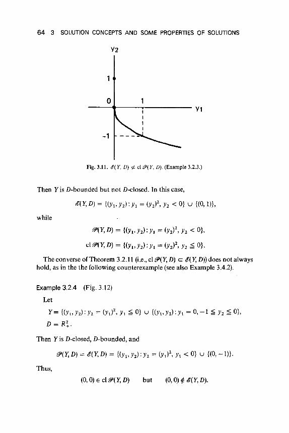
64 3 SOLUTION CONCEPTS AND SOME PROPERTIES OF SOLUTIONS
Y2
1
o 1-----41~--..------- Y1
-1
Fig. 3.11. <&'( Y, D) ¢ cl &'( Y, D). (Example 3.2.3.)
Then Yis D-bounded but not D-closed. In this case,
while
.o/'(Y,D) = {(YI'YZ):YI = (Yz)Z, Yz < O},
cl.o/'(Y, D) = {(YI'Yz):YI = (yz)Z, Yz ~ O}.
The converse of Theorem 3.2.11 (i.e., cl.o/'(Y, D) c: $(Y, D)) does not alwayshold, as in the the following counterexample (see also Example 3.4.2).
Example 3.2.4 (Fig. 3.12)
Let
Y= {(Yl'Yz): Yz = (YI)Z, Yl ~ O} U {(Yl' Y2):Yl = 0, -1 ~ Yz ~ O},
D = R~.
Then Yis D-closed, D-bounded, and
Thus,
(0,0) E cl .0/'(Y, D) but (0,0) ¢ $(Y, D).
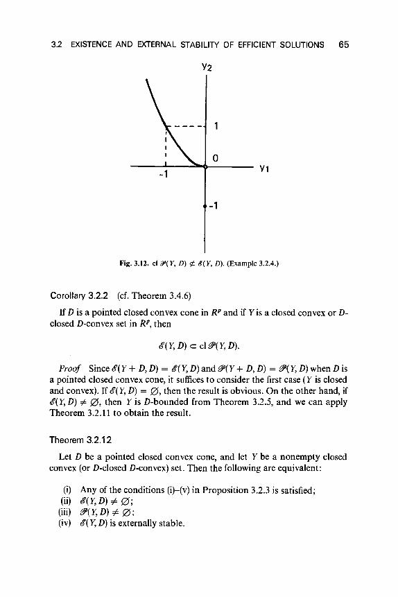
3.2 EXISTENCE AND EXTERNAL STABILITY OF EFFICIENT SOLUTIONS 65
Y2
-1
1
oYl
-1
Fig. 3.12. cl9"(Y, D) ¢ 8(Y, D). (Example 3.2.4.)
Corollary 3.2.2 (cf. Theorem 3.4.6)
IfD is a pointed closed convex cone in RP and if Y is a closed convex or D-closed D-convex set in RP, then
0"(Y, D) c cl &'(Y,D).
Proof Since 0"(Y+ D, D) = 0"(Y, D) and &,(Y + D, D) = &'(Y,D) when Disa pointed closed convex cone, it suffices to consider the first case (Y is closedand convex). If 0"(Y, D) = 0, then the result is obvious. On the other hand, if0"(Y, D) =1= 0, then Y is D-bounded from Theorem 3.2.5, and we can applyTheorem 3.2.11 to obtain the result.
Theorem 3.2.12
Let D be a pointed closed convex cone, and let Y be a nonempty closedconvex (or D-closed D-convex) set. Then the following are equivalent:
(i) Any of the conditions (i)-(v) in Proposition 3.2.3 is satisfied;(ii) 0"(Y, D) =1= 0;
(iii) &'(Y,D) =1= 0;(iv) 0"( Y, D) is externally stable.

66 3 SOLUTION CONCEPTS AND SOME PROPERTIES OF SOLUTIONS
Proof (i) <:> (ii) is shown in Theorem 3.2.5. (i) => (iv) follows fromTheorem 3.2.9 or Theorem 3.2.10. (ii) => (iii) follows from Theorem 3.2.11.Finally, (iii) => (ii) and (iv) => (ii) are trivial.
Some examples of externally unstable sets will be given later in Chapter 4,in connection with the perturbation stability of efficient sets.
3.3 Connectedness of Efficient Sets
In this section we discuss the connectedness of efficient sets in multi-objective optimization problems. Throughout this section, the dominationstructure is given by a constant pointed closed convex cone D. The followingresults are mainly due to Naccache [Nl].
Definition 3.3:1 (Separatedness and Connectedness)
A set A c RP is said to be separated if it can be written as
A = A 1 U Az,
where
cl A 1 n A z = A 1 n cl A z = 0
with two nonempty sets A 1 and A 2 • Equivalently, A is separated if there existtwo open sets 0 1 and O2 such that
If A is not separated, then A is said to be connected.
The following two lemmas are well known and useful in this section.
Lemma 3.3.1
If a set A is connected and
A c B c clA,
then the set B is also connected.
Lemma 3.3.2
If {Ai: i E I} is a family of connected sets such that nieI Ai "# 0, thenUieI Ai is connected.

Now let
and
3.3 CONNECTEDNESS OF EFFICIENT SETS
Sell, Y) = {Y E Y: </l, P) = inf</l,Y>}yEY
!!&(Y, D) = U Sell, Y).u e Int D"
67
From the results given later in Section 3.4 (Theorems 3.4.3 and 3.4.6), wehave the following lemma.
Lemma 3.3.3
!!&(Y,D) c $(Y,D)
and, moreover if Yis closed convex, then
$(Y, D) c cl !!&(Y, D).
We first prove the connectedness of the set !!&(Y, D) in the case in which Yisa com pact con vex set.
Lemma 3.3.4
If Yis a compact convex set, then !!&(Y, D) is connected.
Proof Suppose, to the contrary, that !!&(Y, D) is not connected. Then thereexist two open sets Y1 and Y2 such that
li n !!&(Y, D) #- 0, i = 1,2, Y1 n Y2 n !!&(Y, D) = 0,
!!&(Y, D) C Y1 U Y2 .
Let
Ai = {/l E int DO : Sell, Y) n li #- 0}
Since S(p" Y) is connected by convexity,
Ai = {/l E int DO : Sell, Y) c li}
Hence,
A 1nA2 = 0 ·Moreover, since li n !!&(Y, D) #- 0,
i = 1,2.
i = 1,2.
for i = 1,2,.«, r, intDO #- 0
and since !!&(Y, D) c Y1 U Y2 ,
int DO c Al U .412 (to say exactly int DO = Al U .4(2) ,
68 3 SOLUTION CONCEPTS AND SOME PROPERTIES OF SOLUTIONS
Finally, each Jri is an open set (see Lemma 3.3.5 below). These all imply thatint DO is not connected, which is a contradiction. Therefore ~(Y, D) should beconnected.
Lemma 3.3.5
If Y is compact convex, then the sets
Jri = {Jl E int DO : S(jl, Y) c ~} i = 1,2
in the proof of Lemma 3.3.4 are open.
Proof We will show that Jr. is open. Suppose, to the contrary, that Jr. isnot open. Then there exist fl E Jrl and Jlk E int DO\Jr. = Jr2 (k = 1,2, ...)such that Jlk -+ fl. Take 1 E S(Jlk, Y) (k = 1,2, ...). Since Y is compact we canassume without loss of generality that the sequence {I} converges to anelement yE Y, which is contained in S(fl, Y). In fact, if y¢ S(fl, Y), there existsa y' E Y such that
<fl, y') < <fl, Y)·From the continuity of the inner product we see that for sufficiently large k,
<Jlk, y') < <Il, I),
which contradicts the fact that 1 E S(jlk, Y).Since 1 E S(l, Y) c Y2 n ~(Y, D) and Yl n Y2 n ~(Y, D) = 0, then
1 E Y~ (the complement of Y1) for all k = 1,2, .... Since Yl is a closed set,the limit yof {I} is also in Y1.Thus, we have y¢ Yl , which is contradictorytoflEJrl·
Theorem 3.3.1 t
IfD is a pointed, closed, convex cone and Y is a closed, convex, D-boundedset, then cS'(Y, D) is connected.
Proof Pick
d e int D
and define
y(oe) = «d a E R.
We claim that, for any y E RP, there exists o: > 0 such that
y E y(oe) - D.
t Naccache [NI].
3.3 CONNECTEDNESS OF EFFICIENT SETS 69
If this is not true, then we can apply the standard separation theorem to theray {y - ad: a > O} and the convex cone - D to deduce the existence of/l E RP\{O} such that
</l, y - rxd) ~ 0 for all rx > 0
and
</l, d') ~ 0 foraIl de D,
Since de int D, </l, d) > 0 from the latter inequality and so </l, y - ad) < 0for sufficientlylarge a, which is a contradiction.
We can therefore choose & > 0 such that
(y(&) - D) n S(Y,D) "# 0.
Let
E(rx) = S((y(rx) - D) n Y, D).
The claim proven above shows that
S(Y,D) = UE(rx)."s:a
Since (y(rx) - D) n Y is compact convex from the assumptions (seeProposition 3.2.3), E(rx) is connected from Lemmas 3.3.1, 3.3.3, and 3.3.4.Moreover, if a ~ &, then
E(rx) ::> E(&),
which implies that
nE(a) = E(&) "# 0.,,;;;a
We have therefore expressed S(Y,D) as the union of a family of connectedsets having a nonempty intersection and as such S(Y, D) must be connected.This completes the proof.
Remark 3.3.1
The condition that Y be closed and convex in Theorem 3.3.1 may bereplaced by the assumption that Y is D-closed and D-convex according toProposition 3.1.2.
Bitran and Magnanti [BI4] obtained essentiaIly the same result asTheorem 3.3.1. Warburton [W4] recently obtained connectedness results forthe set of Pareto optimal and weak Pareto optimal solutions in the decisionspace (i.e., x space)..
70 3 SOLUTION CONCEPTS AND SOME PROPERTIES OF SOLUTIONS
3.4 Characterization of Efficiency and Proper Efficiency
In this section we develop characterization theorems for efficient andproperly efficient points. The domination structure is assumed to be specifiedby a convex cone D. The efficient set of Y with respect to D is denoted by$(Y, D) as before; that is,
y E !&'(Y, D) if and only if (Y - y) (1 (-D)
{{a}
- 0 when D does not contain the origin.
Moreover, when D is a closed convex cone, we use 8I'(Y, D) to denote the setof all properly efficient points of Yin the sense of Benson. Namely,
YE &i(Y,D) if and only if cl P(Y + D - y) (1 (-D) = {O}.
Three kinds of characterization are discussed in sequence. Some more resultsnot discussed here can be seen in Gearhart [G4] and Jahn [12].
3.4.1 Characterization by Scalarization
Most well-known results regarding the characterization of efficient orproperly efficient points are via scalarization by vectors in the polar or strictpolar cone of the domination cone. As in Section 3.3, let
S(J1, Y) = {Y E Y:<J1, y) = inf{<J1, y): y E Y}}.
Geometrically, S(J1, Y) is the set of supporting points of Y with the innernormal vector J1. It is obvious that S(IXIl, Y) = S(Il, Y) for any IX > O. Hence,we may often normalize 11 as 111111 = 1. Let
2J(Y, D) = U S(J1, Y)p.eDS O
and
2J(Y, D) = U S(Il, Y)./lEDO\{Oj
Of course, 2J(Y, D) c ~(Y, D).
Proposition 3.4.1
If Y is a closed set, then
cl2J(Y, D) c ~(Y, D).

3.4 CHARACTERIZATION OF EFFICIENCY AND PROPER EFFICIENCY 71
Proof Let Y' E S(/lk, Y) with Ilk E lYO and Y' ~ y. Since we can normalizel as Il/lll = 1, we may assume that Ilk converges to some {t with 11{t11 = 1without loss of generality by taking a subsequence if necessary. Then{t E cl DSOc DO since DSO c DO and DO is closed. Moreover, y E S({t, Y). Infact, since Y' E S(l, Y),
for Vk = 1,2, ... , Vy E Y.
Taking the limit as k ~ 00, we have
<{t,y - y) ;;;; 0 for any y E Y.
Hence y E ~(Y, D), as was to be proved.
We will now investigate the relationships between &!(Y, D) (or 6"(Y, D)) and.@(Y, D) (or ~(Y, D)).
Theorem 3.4.1
If D is a closed convex cone in RP, then for an arbitrary Yin RP,
.@(Y, D) c &(Y, D).
Proof Let /l E DSO and yE Siu, Y). If we suppose that
-d E cl P(Y + D - y) and dED,
as k ~ 00.
then there exist sequences {Y'} c Y, {dk}C D and {Pk} c R such that Pk ;:;; 0
and
Pk(Y' + dk- y) ~ - d
Taking the inner product with u, we have
lim Pk{«/l,Y') - </l,y») + </l,dk) } = -</l,d).
k-+ 00
Since y E S(/l, Y), dk E D, and /l E DSo, the left-hand side is nonnegative. So
</l, d) ;;;; 0,
and hence d = O. Thus we have established that
clP(Y+ D - y) n (-D) = {O},
i.e., y E &(Y, D). This completes the proof.
Theorem 3.4.2
If D is a pointed, closed, convex cone and Y is a D-convex set in RP, then
&!(Y, D) c .@(Y, D).

72 3 SOLUTION CONCEPTS AND SOME PROPERTIES OF SOLUTIONS
Proof Let y E .1P(Y, D), i.e.,
cl P(Y + D - Y) 11 (-D) = {O}.
From Lemma 3.1.1, cl P(Y + D - y) is a closed convex cone. So we canapply Proposition 2.1.8 to obtain that
Dso l1 (cl P(Y + D - y))O =F 0.Thus, there exists a J1 E VO such that
J1 E (cl P(Y + D _ y))o.
Since Y - Yc cl P(Y + D - y),
<J1, y - y) ~ 0 for any y E Y.
Namely,
for all y E Y.
Therefore, yE £&(Y, D), as was to be proved.
Remark 3.4.1
In view of Theorems 3.4.1 and 3.4.2, when D is a pointed closed convexcone and Y is a D-convex set, every properly efficient point of Y can becompletely characterized as a supporting point of Y with an inner normalvector in D"o. This geometric result is quite useful in the dicussion ofmultiobjective duality theory (Chapter 5).
Theorem 3.4.3
IfD is a convex cone and Y is a set in RP, then
£&(Y, D) c G(Y, D).
Proof Suppose that y¢ G(Y, D). If Y¢ Y, it is clear that y¢ £&(Y, D). Soassume that y E Y\G(Y,D), and there exists a y' E Y such that y - y' E D\{O}.Then for any J1 E D"O,
<J1, y - y') > O.
Thus Y¢ £&(Y, D), as was to be proved.
Theorem 3.4.4
If D is an acute convex cone and Y is a D-convex set in RP, then
G(Y, D) c ~(Y, D).
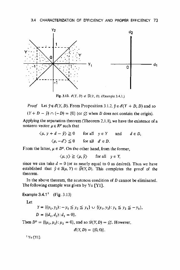
3.4 CHARACTERIZATION OF EFFICIENCY AND PROPER EFFICIENCY 73
o----1----- dl
Fig. 3.13. B(Y, D) ¢ :@(Y, D). (Example 3.4.1.)
Proof Let pe tt(Y, D). From Proposition 3.1.2, pe tt(Y + D, D) and so
(Y + D - y) n (-D) = {O} (or 0 when D does not contain the origin).
Applying the separation theorem (Theorem 2.1.1), we have the existence of anonzero vector /1 e RP such that
</1, Y + d - y) ~ 0
</1, -d') ~ 0
for all Y e Y and
for all d' e D.
deD,
From the latter, /1 e DO. On the other hand, from the former,
</1, y) ~ (/1, y) for all ye Y,
since we can take d = 0 (or as nearly equal to 0 as desired). Thus we haveestablished that ye S(/1, Y) c .@(Y, D). This completes the proof of thetheorem.
In the above theorem, the acuteness condition of D cannot be eliminated.The following example was given by Yu [Yl].
Example 3.4.1 t (Fig. 3.13)
LetY= {(Yl,Yz):-Yl ~ Y2 ~ Yl} U {(Yl,Yz):Yl ~ Y2 ~ -Yl}'
D = {(dl , d2 ) : dl = O}.
Then DO = {(/1l' /12): /12 = O}, and so .@(Y, D) = 0. However,
tt(Y,D) = {(O} on.t Yu [Yl].

74 3 SOLUTION CONCEPTS AND SOME PROPERTIES OF SOLUTIONS
Corollary 3.4.1
Let D be an acute, open, convex cone and Ybe a D-convex set in RP. Then
Iff(Y, D) = ~(Y, D).
Proof In view of Proposition 2.1.5(iv), DSO = DO\{OJ when D is open.Hence !!tJ(Y, D) = .@(Y, D), and the corollary directly follows from Theorems3.4.3 and 3.4.4.
An element in S(Ji, Y) is not necessarily efficient for Ji E DO, in contrast withTheorem 3.4.4. However, we can at least claim the following.
Theorem 3.4.5
Let D be an acute, convex cone and Y be a set in RP. If Ji E DO andS(Ji, Y) = {y}, then y E <&'(Y, D). If Y is nonempty and compact, then for anyJi E DO, S(Ji, Y) () <&'(Y, D) i= 0.
Proof If y¢ 1ff(Y, D), there exists y' i= yin Ysuch that y - y' ED. Then<Ji, y - i) ~ 0, which implies that S(Ji, Y) i= {Y}.
Next, assume that Y is nonempty and compact. Then, for any Ji E DO,S{J1, Y) is a nonempty, compact set, and hence there exists YE <&,(S(Ji, Y),D)from Theorem 3.2.2 and Remark 3.2.2. Then YE 1ff(Y, D). In fact, if there werey' E Y such that y - i E D\{O}, then the inequality <Ji, y) ~ <Ji, i) holds.Therefore, i E S(Ji, Y), which contradicts the supposition y E <&'(S(jl, Y), D).Thus YE S(jl, Y) () <&'( Y, D), and the proof of the theorem is completed.
The following theorem, which is a generalization of a theorem of Arrow etal. [A4], is due to Hartley [H5].
Theorem 3.4.6 (cr. Corollary 3.2.2)
IfD is a pointed closed convex cone and if Yis a closed, convex set or if YisaD-closed, D-convex set, then
<&'(Y, D) c cl !!tJ(Y, D) = cl &'(Y, D).
Proof Theorems 3.4.1 and 3.4.2 ensure that
cl!!tJ(Y,D) = cl&'(Y,D)
in this case. Hence, the result follows immediately from Corollary 3.2.2.However, we will give a direct proof of the relationship. Hence we provethat <&'(Y, D) c cl !!tJ(Y, D). Since <&'(Y + D, D) = 1ff(Y, D) and !!tJ(Y, D) =2t1(Y + D, D), it sufficesto prove the first case (Yis a closed convex set). If Yisempty, the theorem is trivial, and so we assume that there is y E <&'(Y, D). Wecan take y = 0 for simplicity without loss of generality.

3.4 CHARACTERIZATION OF EFFICIENCY AND PROPER EFFICIENCY 75
First we prove the case in which Y is compact and convex. Choose ji E DSO
and let C(e) = eji + DO for any e > O. Then, for all e sufficiently small, YandC(6) n B are both nonempty, compact, and convex, where B is the closedunit ball. Hence, by the minimax theorem of Sion-Kakutani (Stoer andWitzgall [SIS]), there exist y(e) E Yand f.1.(6) E C(6) n B such that
<f.1., Y(6) ;;; <f.1.(6), Y(6) ;;; <11(6), y) for v» E Y, 'ill E C(6) n B.
Since 0 E Y, we have
<11, Y(6) ;;; 0 for all 11 E C(6) n B.
Since Y is compact, there exists a sequence of positive numbers {13k}
converging to 0 such that the sequence {I} = {y(ek)} has a limit y E Y as
k ~ 00. For any 11 E DSOn B = (int DO) r, B, we can find an e> 0 such thatf.1. E C(e) n B for all 6 ;;; e, and thus <Ji, I) ;;; 0 for all large enough k. SinceDSO is a cone, this implies that
for all f.1. E DSO
and thus
-y E (VSO)O = D.
Because 0 E g( Y, D), Y = 0 and defining
,l = l1(ek)/IIf.1.(~)11 E DSO naB,
we have
1 E S(Jik, Y) c 22(Y, D).
Now suppose Y is not necessarily compact (but closed and convex). LetoE g(Y, D). Since Y n B is a nonempty, compact, convex set andoE g(y r. B, D), from the above result there exist sequences {f.1.k} c VSO with11,l11 = 1 and 1 E S{f.1.k, Y n B) such that 1 ~ O. If k is sufficiently large,1 E int B and thus 1 E S(I1k, Y). In fact, if there were y' E Y such that
<Ilk,y') < <f.1.k, I),
then IXy' + (1 - IX)I E Y n B for sufficiently small IX > 0 and
<,l, IXy' + (1 - IX)/) < <,l, I),
which contradicts 1 E S(f.1.\ Y n B). This completes the proof of thetheorem.
In this theorem, the converse inclusion g(Y, D) ~ cl g1i(Y, D) does not holdgenerally as can be seen in the following example.
76 3 SOLUTION CONCEPTS AND SOME PROPERTIES OF SOLUTIONS
Example 3.4.2 t
Let
y' = {(Yl, Y2' Y3): (Yl - 1)2 + (Y2 - 1)2 = 1, Yl ~ 1, Y2 ~ 1, Y3 = I},
Y = co(Y' u {(I, 0, Om,
D = R~.
Then Y is closed and convex, and y = (1,0,1) ¢ tff(Y, D), sincey = (1,0,0) + (0,0,1). However any Y E Y' such that Yl < 1, Y2 < 1 iscontained in &'(Y, D) = ~(Y, D). In fact, if we put
then
y = (1 - cos e, 1 - sin e, 1) for °< e < 1-,
Il = (1 - a)(cos e, sin 0,0) + a(O,O, 1), O<a<1
is in lY O and, for any Y E Y' with Y = (1 - cos 0', 1 - sin 0', 1),°~ 0' ~ 1-,
<Il, Y - y) = (1 - a){(cosO)(cos e- cos 0') + (sin O)(sin 0 - sin O')}
= (1 - a){1 - cos(O - O')} ~ 0.
Moreover,
<Il, (1, 0, 0) - Ji) = (1 - a) cos" 8 - (1 - a) sin 8(1 - sin 8) - a
= (1 - a)(1 - sin e) - a > 0
for any a sufficiently small. Thus
<Il, Ji) ~ <Il, y) for all Y E Y
and so y E ~(Y, D). Letting e- 0, we find y E cl ~(Y, D).
When Y is a polyhedral convex set, we obtain the following result.
Theorem 3.4.7
If Yis a polyhedral convex set and D is a pointed closed convex cone, then
&'(Y,D) = tff(Y, D) = ~(Y, D).
Proof The theorem is obvious from Theorems 3.1.7, 3.4.1 and 3.4.2.
t Arrow et al. [A4].
3.4 CHARACTERIZATION OF EFFICIENCY AND PROPER EFFICIENCY 77
3.4.2 Characterization as Best Approximations to the Ideal Point
In this subsection we concentrate on compromise solutions to multi-objective optimization problems. The domination structure is assumed to bespecified by the nonnegative orthant R~. In other words, we pay attention tothe Pareto optimal points. The idea of compromise solutions is based on aprocedure that calculates the Pareto optimal points as approximations to anideal or utopia point (Yu and Leitmann [Y3], Zeleny [Z3], Bowman [B20],Gearhart [G3], Salukvadze [S3]). We investigate the relationships betweencompromise solutions and efficient (or properly efficient) points partlyaccording to Gearhart [G3].
We consider a multiobjective optimization problem
(P) minimize f(x) = Ui(X), .. ·,fix» subject to x E X C W
with the domination structure D = R~. Therefore, our aim is to find the setof all Pareto optimal points (or solutions). Since D is fixed, the efficient set ofY = f(X) is simply denoted by $(Y). We assume that the set Y + R~ is closed(i.e., Y is R~ -closed) and that
Yi = inf{J;(x): x E X} > -00
for each i = 1, ... , p. The point Y = (Yi' ... ,h) is often called the utopiapoint or the ideal point. However, we might take another ideal point ji asji ~ y.
The loo-norm in W is defined by
Ilyll 00 = max{IYil : 1 ~ i ~ p}, YEW.
Let A be a scalar index set bounded below and unbounded above (a simpleexample is A = [1, (0)) and let a family of norms {II·IL.: oc E A} be givenwhich has the following properties:
Property P1: Ilylloo ~ M(oc)llyll", with M(oc) > 0, oc E A, YEW,
Property P2: M(oc)llyll", --+ Ilylloo as oc --+ 00, Y E RP
Property P3: if 0 ~ Y s y', then Ilyll", < 1Iy'11", for each oc E A.
Example 3.4.3
(i) The most popular example of such families is that of the I.-norms,i.e.,
Ilyli. = [tiIY;I"'T/"',In this case M(oc) = 1.
oc E [1, (0).

78 3 SOLUTION CONCEPTS AND SOME PROPERTIES OF SOLUTIONS
(ii) Another example, which was used by Dinkelbach and Isermann[D6], is given by
a E [1,00).
for aE(I,oo).
In this case M(a) = 1.(iii) The final example was proposed by Choo and Atkins [ClO]. Let I~
be the P x P matrix whose (j, k) entry is given by
{I ifj=k
(I~)jk = -1/(p - l)a if j =F k
Then I~ is nonsingular and
(I-1). = {a((p - l)(a - 1) + 1)/(a - 1)((P - l)a + 1)a Jk al(a - 1)((P - l )« + 1)
Here every component is positive and
(I;1)jj = [(P - 1)(a - 1) + 1](I;1)jk > (I;1)jk
We define
In this case
if j = k
if j =F k.
(j =F k).
Iy;i = 1(I~I;1y);i ~ I(I;1y);i + Ct11(I;1Y)jl)!(P - 1)a.
HiHence
where M(a) = 1 + l/a.Let SP be the set as follows:
SP = {Jt E RP:J/i = 1, Jti > 0 (i = 1, ... , P)}.
For each u ESP and a E A, the (Jt, a)-norm of y E RP is defined by
Ilyll~ = IIJt (0 yll~,
and the (Jt, 00 )-norm is defined by
Ilyll~ = IIJt (0 yiLt>,where Jt (0 Y = (Jt1Y1'" ·,JtpY p)·
3.4 CHARACTERIZATION OF EFFICIENCY AND PROPER EFFICIENCY 79
In this subsection ji E RP will designate a fixed but arbitrary point suchthat ji ~ y. This point will serve as the ideal point. Define
A(Il, IX, Y) = {,Y E Y: II; - jill~ = inf{lIy - jill~: y E Y}},
i.e., A(Jl, IX, Y) is the set of best approximations to ji out of Y in the (J.L, IX)-norm. Moreover, denote by dey) the set Upd~"EA A(Jl, IX, Y), i.e., dey) isthe set of all best approximations to ji out of Y in the (Jl, IX)-norm for someu E SP and IX EA.
Definition 3.4.1 (Compromise Solution)
A point ji in dey) is called the compromise solution (in the objective space)to the multiobjective optimization problem (P).
We now investigate the relationships between dey) and c&"(Y) (or &'(Y».
Theorem 3.4.8
If Yis R~ -closed and the family of norms {11·110:: IX E A} satisfies PropertiesPI-P3, then
dey) c &,(Y) c c&"(Y) c cl d(Y).
Proof Since &'(Y) c c&"(Y), we will prove that dey) c ,qIl(Y) andc&"(Y) c cl dey).
(d(Y) c &'(Y»: First, let ; E deY). Then for some Jl E SP and IX E A,
liP - jill~ ~ Ily - jill~ for all y E Y.
Suppose to the contrary that PIf &'(Y). Then there exist sequences {Pk} c R,{yk} c Y, {dk
} C R~ such that Pk > 0 and
for some nonzero d E R~.
There are two cases for {Pk}: bounded and unbounded. If {Pk} is bounded wemay assume, without loss of generality (by taking a subsequence if necessary)that Pk -> Po for some Po ~ O. IfPo = 0, noting that yk + dk
- P~ ji - y, wehave -d E (ji - Y+ R~t = R~, which is a contradiction. If Po > 0,t + dk - Y-> -dlPo =1= 0 E -R~ as k -> 00. Since Y + R~ is closed,P- dlPo E Y + R~, i.e., there exists yO E Ysuch that y 2 yo. However, thisimplies that
liP - .vll~ > Ilyo - jill~
by Property P3 and leads to a contradiction.
80 3 SOLUTION CONCEPTS AND SOME PROPERTIES OF SOLUTIONS
If {fJk} is unbounded we may assume that, fJk --+ 00 as k --+ 00. HenceI + dk
- P--+0. If Pi = .vi for some i, then d, = O. In fact,
fJk(Y; + df - .vi) ~ fJk(Yi + df - .vi) = fJkdf ~ 0
for this i and so - d, ~ O. Thus, there exists a p> 0 such that
o ~ y - dlfJ - Y ~ y - YThen, from Property P3,
liP - dlfJ - ylI~ < liP - yll~
for all fJ ~ p.
for all fJ ~ p.Since fJk --+ 00, then fJk ~ Pfor all k sufficiently large. Hence,
III + dk- YII~ < liP - jill~
for some k sufficiently large. In fact,
III + dk- YII~ = III + dk- P+ dlfJk + P- dlfJk - jill~
~ III + dk- 911~ + Ildll~/fJk + 119 - dlfJk - yll~
and the first and second terms of the right-hand side converge to 0 as k --+ 00.
Thus, we have
III - yll~ < 119 - YII~
for some k sufficiently large, since I + dk- ji ~ I - ji ~ O. This is also a
contradiction and therefore 9 E .9(Y).(tS'(Y) c cl d(Y)): Let 9 E tS'(Y). We will prove that for each 8 > 0, there
exists y(t) E d(Y) such that lilt) - 91100 < 8. First, there exists y' > y suchthat
lIy - Plloo < s for any y E(Y' - R~) n Y.
In fact, if no such y' exists, then there exists a sequence {r} c RP such thatr > y, r --+ 9 and for each k, there is a IE (1 - R~) n Y such that11/- Pll oo ~ 8. Since Y + R~ is closed and Y is R~-bounded, we mayassume without loss of generality that I --+ r" + dO with yO E Yand dO ~ 0.Then
IIYo + dO - ylloo ~ 8.
However, r" + dO E (y - R~) n (Y + R~) = {9}, since y E tS'{Y). Thus, wehave a contradiction.
Now, since ji ~ 9 < y', there exist some p E SP and fJ > 0 such that
y' - Y= fJ(1/PI' ... , 1/pp) '
Then
i = 1, .. . ,p.

3.4 CHARACTERIZATION OF EFFICIENCY AND PROPER EFFICIENCY 81
Hence, 119 - yll~ < {3. Let y(a) be a best approximation to y out of Yin the(11, a)-norm. Since Y+ R~ is closed, y(a) exists. Then, from Property PI,
lIy(a) - yll~ ~ M(a)lly(a) - YII~ ~ M(a)119 - YII~.
From Property P2, for all a sufficiently large,
lIy(a) - YII~ ~ {3,
whence
for all i = 1, ... , p,
i.e., y(a) ~ y'. Thus y(a) E (y' - R~) n Y, and so if we put l£) = y(a) forsufficiently large a, there I!y(£) - 91100 < e. This completes the proof of thetheorem.
Remark 3.4.2
The proof of Theorem 3.4.8 suggests that, in order to generate the efficientset, the value of a should be taken large. However, as has been established asTheorem 3.4.6, it suffices to use the so-called [I-norm [i.e. a = 1 in the normof Example 3.4.3(i)] only if Yis R~ -convex. Possibly, the magnitude of a thatis required can be related to a measure of the nonconvexity of Y.
Remark 3.4.3
(i) In Theorem 3.4.8, the converse relationship t&'(Y) ::> cl d(Y) does notnecessarily hold. In fact, if
and Y = (-1, -1), then 9 = (0,0) ¢ tS'(Y), but 9 E cl t&'(Y) c cl d(Y) (see Fig.3.14).
(ii) On the other hand, the relationship d(Y) ::> &(Y) holds when y < yand we use the family of norms (ii) or (iii) in Example 3.4.3. This fact will beshown later in Theorem 3.4.10.
In subsection 3.4.1 we studied the characterization of efficient sets byscalarization. If we use the [I-norm in Example 3.4.1(i), then
8(11, Y) = A(I1, 1, Y).
Namely, the procedure of best approximation by the [I-norm is of particularinterest, though it cannot generate all the efficient points without convexity

82 3 SOLUTION CONCEPTS AND SOME PROPERTIES OF SOLUTIONS
' ..
, .
• to •
\ .. ..
. .
y
I\'Y '.
-1,II
.. - - - -1---------Y -1
Fig. 3.14. <f( Y) +0 cl .w( Y). (Remark 3.4.3(i).)
assumption. We next consider the method of best approximations by theloo·norm (Tchebyshev norm). Let
A oo(j1, Y) = {Y E Y: IIY - yll~ = inf{ Ily - YII~ : y E Y}}
and
Theorem 3.4.9
If Yis nonempty and R~ -closed, then
(i) A oo(j1, Y) n C(Y) "# 0 for each j1 ESP.(ii) C(Y) c cl(doo(Y) n C(Y)). Furthermore, if y < y, then C(Y) c
doo(Y)'
Proof
(i) Since Yis R~-closed, A oo{J1, y) is not empty. In fact, let {l} c Ybe asequence such that
Ill- yll~ -> inf{lly - YII~: y e Y}.

3.4 CHARACTERIZATION OF EFFICIENCY AND PROPER EFFICIENCY 83
Then, we may assume without loss of generality that l -+ yO. Since Y + R~
is closed, yO = / + d for some y' E Yand d E R~. Then
o ~ y' - ji = yO _ ji _ d ~ yO _ y,
11/ - jill~ ~ IIYo - yll~ = inf'[lly - yll~: y E Y}.
Hence, / E A oc,(/1 , Y). Now, let
and let LV} c Aoo(/l, Y) be a sequence such that Lf=1 y~ -+ J. Then we mayassume that yk converges to some y, since Aoo(/l, Y) is bounded. We can provethat y E Aoo(/l, Y) + R~ as before. Then, it is clear thatyE g(Y, D) n Aoo(/l, Y).
(ii) Let y E g(y) and take an arbitrary e > O. Then, as in the proof of thelatter half of Theorem 3.4.8, we can find y' E RP, /l ESP, and 13 > 0 such that
and
Ily - Ylloo < s forany yE Y
y' - ji = f3(1//l 1, .•• , 1//lp) ,
11.v - YII~ < 13·
such that y ~ y',
From the first section of this theorem, there exists yoo E Aoo(/l, Y) n g(y).Then
lI yoo - yll~ ~ Ily - jill~ < 13
and so yoo ~ y'. Therefore Ilyoo - .vII 00 < e, which implies that
.v E cl(doo(Y) n g(y)).
Finally, if ji < y, a given y E g(y) clearly belongs to the set Aoo(/l, Y), where
o< y - ji = f3(1//l 1, ••• , 1//lp)
In fact, if there exists y E Y such that
with 13 > 0,
for every i = 1, ... , p,
then y < y, which is a contradiction, and the proof of the theorem iscompleted.
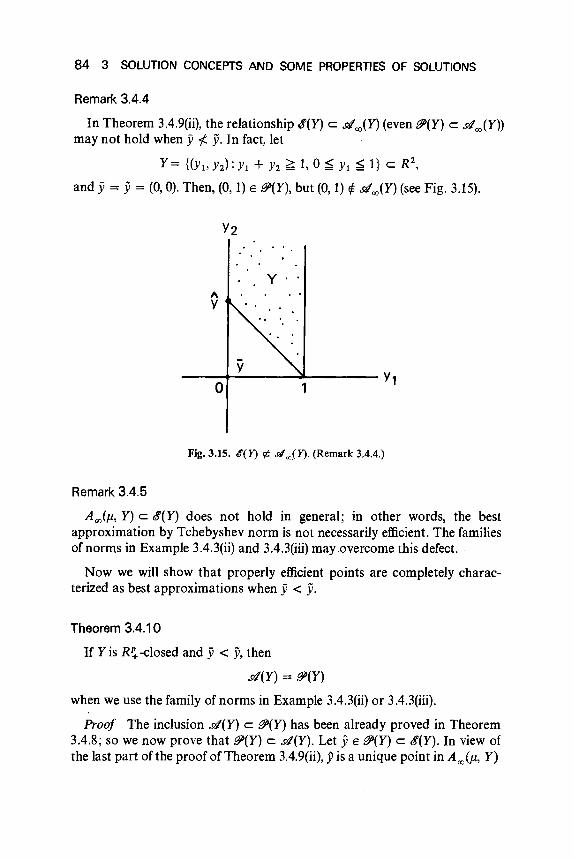
84 3 SOLUTION CONCEPTS AND SOME PROPERTIES OF SOLUTIONS
Remark 3.4.4
In Theorem 3.4.9(ii), the relationship $(Y) c d CXl(Y) (even &I(Y) c d CXl(Y»may not hold when y 1. y. In fact, let
Y= {(Yl'Y2):Yl + Y2 ~ 1,°~ Yl ~ I} C R2,
and y = y = (0,0). Then, (0, 1) E &I(y), but (0,1) 1- dCXl(Y) (see Fig. 3.15).
. , y ..II.Y
1o---+----~---- Y,
Fig. 3.15. <f(Y) ¢ .91",(Y). (Remark 3.4.4.)
Remark 3.4.5
ACXl(p, Y) c cS'(Y) does not hold in general; in other words, the bestapproximation by Tchebyshev norm is not necessarily efficient. The familiesof norms in Example 3.4.3(ii) and 3.4.3(iii) may overcome this defect.
Now we will show that properly efficient points are completely charac-terized as best approximations when y < y.
Theorem 3.4.10
If Y is R~ -closed and y < y, then
dey) = &I(Y)
when we use the family of norms in Example 3.4.3(ii) or 3.4.3(iii).
Proof The inclusion dey) c &I(Y) has been already proved in Theorem3.4.8; so we now prove that &I(Y) c dey). Let y E &I(Y) c cS'(Y). In view ofthe last part of the proof of Theorem 3.4.9(ii),Pis a unique point in ACXl(/-l, Y)
3.4 CHARACTERIZATION OF EFFICIENCY AND PROPER EFFICIENCY 85
Let {ock } be a sequence diverging to + 00. If'p ¢ dey), we can take a sequence{yk} c Ysuch that
119 - yll~k > III - jill~k for all k = 1,2, ....
Since
M(ock)119 - yll~k > M(ock)111' - yll~k ~ III - yll~
by Property PI and the left-hand side converges to 119 - yll~ as k - 00 byProperty P2, then {I'} is a bounded sequence. Therefore, we may assumewithout loss of generality that 1- y for some y. Since Y is R~-closed,y = y' + d for y' E Yand d E R~. Then, by taking the limit of
M(OCk)119 - yll~k > III' - yll~
as k - 00, we have
119 - yll~ ~ 1Iy' + d - yll~ ~ 1Iy' - yll~
by Property P3. Since 9is an unique point in Aoo(Jl, Y), Y = y' = 9;in otherwords, 1- y. Let dk = f3(1' - y)llll' - PII~. Then y + dk ~ ji and we canprove that
liP + dk- yll~k < liP - yll~k'
In fact, when we use the family of norms (ii) of Example 3.4.3,
1liP + dk
- yll~k = liP - ji + dkll~ + - LJli(Y, - Yi + d~)IX,k I
= liP - yll~k + f3[m~x{JliM - Yin
+ ~ L Jli(Y~ - Yi)]/llyk - YII~.OCk i
Since
119 - jill~k > III' - yll~k = III' - Y+ Y- jill~k
= liP - yll~ + [m~x{Jl,(y~ - Yi)}
+ ~ LJli~ - PI)]'OCk i
the second term of the last equation is negative and therefore
IIY + dk- jill~k < IIY - jill~k'

86 3 SOLUTION CONCEPTS AND SOME PROPERTIES OF SOLUTIONS
Similarly, when we use the family of norms (iii),
Ily + dk- jill~k = III;.l(.u 0 (y - ji)) + Ia~l(.u 0 dk)lloo·
Since
11/- jill~k = III;.l(.u 0 (y - ji)) + I;.l(.u 0 (/- y))lloo
< Ily - jill~k = III;.l(.u 0 (y - ji))lloo
and
we have
Hence
Now, since Ildkll:::' = fJ for any k, we may assume that {dk} converges to some
awith Ilall:::' = fJ. Then, taking the limit of
Ily + dk - YII:::' ~ M(Ctk)lly + dk - jill~k < M(Ctk)lly - jill~k'
we have
Ily + a- jill:::' ~ Ily - jill:::'.
This implies that a~ 0, since y + a~ ji and .u 0 (y - ji) = (fJ, ... ,fJ). Onthe other hand, from the definition of {dk
} , dE cl P(Y + R~ - Y). However,this contradicts the assumption y E &'(Y) and the proof of the theorem iscomplted.
3.4.3 Characterization as Solution of Constraint Problems
Another method of characterizing Pareto optimal solutions is to solve kthobjective constraint problems associated with the original multiobjectiveoptimization problem. The kth objective constraint problem is formulatedby taking the kth objective functionj, as the objective function and letting allthe other objective functionsfj U# k) be inequality constraints (Benson andMorin [BIO], Haimes et al. [H2], Chankong and Haimes [C5, C6]). That is,given the original multiobjective optimization problem
(P) minimize f(x) = (fl(X), ... ,fix) subject to x E X c R",

3.4 CHARACTERIZATION OF EFFICIENCY AND PROPER EFFICIENCY 87
the kth objective constraint problem can be defined as a scalar optimizationproblem
minimize fk(X)
subject to J;(x) ~ ei , i = 1, ... , p, i #- k, x E X,
where s = (e1 , ••• , ep) E RP. A similar type of equality-constrained problemswas studied by Lin [L6-L8].
The following theorems provide the relationships between the Paretooptimal solutions of the original multiobjective optimization problem (P)and the solutions of the kth objective constraint problems (Pk(e)).
Theorem 3.4.11
A point xis a Pareto optimal solution of (P) if and only ifxsolves (Pk(e)) forevery k = 1, ... , P, where e = f(x).
Proof Ifxis not a Pareto optimal solution of (P), there exists x E X suchthat J;(x) ~ J;(x) with the strict inequality holding for at least one k. Thisimplies that xdoes not solve (pk(e)). Conversely ifxdoes not solve (Pk(e)) forsome k, then there exists x E X such thatf,.(x) <fk(X) andJ;(x) ~J;(x) (i #- k),implying that xis not a Pareto optimal solution of (P).
Theorem 3.4.1 2
Ifxis a unique solution of (Pk(e)) for some k E {I, ... , p} with e = f(x), thenxis a Pareto optimal solution of (P).
Proof Since xuniquely minimizes (Pk(e)), for all x satisfying J;(x) ~ J;(x)(i #- k),fk(X) > f,.(x). Hence x is a Pareto optimal solution of (P).
As has been already stated, every properly efficient solution (in the sense ofGeoffrion) is a Pareto optimal solution, but not vice versa in general. Bensonand Morin showed that the converse holds when the constraint problems arestable as scalar optimization problems.
Definition 3.4.2 (Perturbation Function)
The perturbation function W k: RP-1 --+ R = [- 00, + 00] associated with(Pk(e)) is defined as
wk(u) = inf{fk(x):J;(x) - ei ~ u., i = 1, ... , k - 1,k + 1, ... , p, X EX},

88 3 SOLUTION CONCEPTS AND SOME PROPERTIES OF SOLUTIONS
Definition 3.4.3 (Stability)
(Pie)) is said to be stable when Wk(O) is finite and when there exists a scalarM > 0 such that, for all u '# 0,
[wk(O) - wk(u)J/llull ~ M.
Theorem 3.4.13
Assume that f1(x), ... ,fr,(x) are convex functions on the nonempty convexset X and that x is a Pareto optimal (i.e. efficient) solution of themultiobjective optimization problem (P). Then x is a properly efficientsolution of (P) if and only if (Pk(e)) is stable for each k = 1,... , p, wheree = f(x).
Proof Assume first that (Pk(e)) is stable, and then define the dual problemof (Pk(e)) by
(Ok(e)) CPk = max{min[J,.(X) + L j1.U;(x) - ei)]}I'~O XEX ii'k
where j1. is a (p - I)-vector of dual variables. Since (Pk(e)) is stable, adapting aresult of Geoffrion [G6, Theorem 3], we find that (Ok(e)) has an optimalsolution Po and x is an optimal solution for the problem
(P~.I') miminize J,.(x) + L Po;</;(x) - ei ) subject to x E X.ii'k
Since - LPoiei is constant for all x E X, x is an optimal solution of theproblem
minimize J,.(x) + L Po;/;(x)ii'k
subject to x E X.
By Lemma 3.4.1 below, x is a properly efficient solution of (P).Conversely, suppose that x is a properly efficient solution of (P). Then, for
each k = 1, .. .,p there exists (by Lemma 3.4.1) a Po E R~-1 such that x is anoptimal solution of (Pk ,11)' This implies that x is an optimal solution of (P~,Il)'
where (P~,Il) is given above. Thus (x, P) is feasible in (Ok(e)), and so CPk ~ !,,(x).Furthermore, since x is an optimal solution of (Pk,ll) with the optimalobjective value J,.(x), then CPk ~ J,.(x) from the weak duality theorem fornonlinear programming. Thus, CPk = !,,(x), and (x, P)is an optimal solution to(Ok(e)). By Geoffrion [G6], (Pk(e)) is stable. This completes the proof of thetheorem.
Lemma 3.4.1
Suppose that f1(X), ... ,fix) are convex functions on the convex set X.Then x is a properly efficient solution for (P) if and only if, for each k, there
3.5 KUHN-TUCKER CONDITIONS FOR MULTIOBJECTIVE PROGRAMMING 89
exists a u = (ttl'" .,ttk-l,ttk+l'" .,ttp) E R~-l such that x is an optimalsolution of the problem (Pk,/J
Proof This result is obvious from Theorems 3.4.1 and 3.4.2.
Remark 3.4.2
Though stability may not be an easy property to demonstrate directly, itholds whenever some constraint qualification (e.g. Slater's constraint quali-fication) is satisfied. (See Geoffrion [G6].)
Details concerning the constraint problems can be found, for example, inChankong and Haimes [C6]. The interested reader may refer to it.
3.5 Kuhn-Tucker Conditions for Multiobjective Programming
In this section we deal with the Kuhn-Tucker condition for a multi-objective programming problem
(P) minimize f(x) = (fl(X), ... ,fp(xW
subject to x E X = {x E RR:g(x) = (gl(X), ... , gm(xW ~ O}.
Here the domination structure is given by a convex cone D, in particular R~.
The necessary and/or sufficient conditions for efficiency (or Pareto opti-mality) in this problem have been studied by a number of researchers (Kuhnand Tucker [K10], Hurwicz [H16], DaCunha and Polak [D1], Neustadt[N14j, Ritter [R4-R6], Smale [S10, Sll], Wan [W3], Tamura and Miura[T4]). In this section we derive necessary/sufficient conditions for Paretooptimality under the assumption that every /; (i = 1, ... , p) and gjU= 1, ... , m) is continuously differentiable. Results under the convexityassumption are closely related to the duality theory and so will be discussedfully in later chapters.
Theorem 3.5.1
A necessary condition for xE X to be a properly efficient solution to (P) inthe sense of Kuhn-Tucker is that there exist AE RP and ~ E B" such that
(i) <A, Vf(x) + <~, Vg(x) = 0.(ii) <~, g(x) = 0,
(iii) A> 0, ~ ~ 0,
where <A, Vf(x) and <~, Vg(x) stand for Lf=l Ai V/;{x) and 2:j=l ~j VgJ{x),respectively.

90 3 SOLUTION CONCEPTS AND SOME PROPERTIES OF SOLUTIONS
Proof From Kuhn-Tucker's definition of proper efficiency (Definition3.1.10), there is no h E R" such that (Vflx), h) ~ 0 (i = I, ... , p) with thestrict inequalities for at least one i and that
j E lex) = {j: gix) = O}.
Then, from the Tucker's theorem of alternatives (Mangasarian [M2J), thereexist it; > 0 (i = I, ... , p) and ~j ~ 0 UE lex)) such that
p
L iti V/;(x) + L: ~j Vgix) = 0i= 1 jeJ(x)
Letting ~j = 0 for j rt: lex), we can immediately establish the theorem.
Corollary 3.5.1
If the Kuhn-Tucker constraint qualification is satisfied at xE X, anecessary condition for x to be a properly efficient solution to (P) in the senseof Geoffrion is the condition in Theorem 3.5.1.
Proof Immediate from Theorem 3.1.6 and 3.5.1.
Theorem 3.5.2
If every function /; (i = 1, ... , p) and gj U = 1, ... , m) is convex, thecondition in Theorem 3.5.1 is also sufficient for xE X to be a properlyefficient solution to (P).
Proof The condition in Theorem 3.5.1 implies that f(x) E S(P, Y) (seeSection 3.4.1) and hence, from Theorem 3.4.1, x is a properly efficientsolution of (P).
Theorem 3.5.3
Suppose that (P) satisfies the Kuhn-Tucker constraint qualification atxEX. Then, a necessary condition for x to be a weak Pareto optimalsolution to (P) is that there exist it E RPand ~ E B" such that
(i) (it, Vf(x» + <~, Vg(x» = 0,(ii) <Jc, g(x» = 0,
(iii) it;;::: 0, ~ ~ O.
Proof Let xbe a weak Pareto optimal solution of (P). We prove thatthere is no h such that
<V/;(X), h) < 0
(Vgix), h) ~ 0
i = 1, .. . ,p,
j E lex) = {j:gix) = OJ.
3.5 KUHN-TUCKER CONDITIONS FOR MULTIOBJECTIVE PROGRAMMING 91
Then the theorem follows from Motzkin's theorem of alternatives(Mangasarian [M2]). Suppose, to the contrary, that there exists an hsatisfying the above inequalities. From the Kuhn-Tucker constraint quali-fication, there exists a continuously differentiable arc (J(t) (0 ~ t ~ t) suchthat (J(O) = x, g«(J(t» ~ 0 and 0(0) = Cl.h (CI. > 0) as
/;«(J(t» = /;(x) + t<V/;(x), Cl.h) + oCt).
Since <V/;(x), h) < 0 for all i = 1, ... , p, then /;«(J(t» < /;(x) for t sufficientlysmall. This contradicts the weak Pareto optimality of X, as was to be proved.
Theorem 3.5.4
If every function /; (i = 1, ... , p) and gj U= 1, ... , m) is convex, thecondition in Theorem 3.5.3 is also sufficient for xE X to be a weak Paretooptimal solution to (P).
Proof The condition in Theorem 3.5.3 implies thatf(x) E S(it, Y), whereit E R~\{O}. Since, in view of Corollary 3.4.1, S({t, Y) c <9'(Y,intR~) underthe convexity assumption, xis a weak Pareto optimal solution of (P).
Remark 3.5.1
Tamura and Miura [T4] obtained efficiency conditions for the case wherethe domination cone D is a polyhedral convex cone. However, that case canbe reduced to the case D = R~ (cf. Lemma 2.3.4). In fact, if D is given as
D = {d E W: <bi, d) 60, i = 1, ... ,/},
thenf(x) - f(x') E D for x, x' E X if and only if
<bi,f(x) - f(x'» ~ 0, i = 1, ... , I,
for i = 1, ... , I,
i.e., if and only if
<bi,f(x» - <bi,f(x'» ~ 0
Therefore, by putting
];(x) = <bi,f(x»
for i = 1, ... , I.
we can essentially identify the original problem (P) with a new I-objectiveoptimization problem
minimize lex) = (h(x), ... ,hex»~ subject to x E X.
Remark 3.5.2
In the above discussion we assume the continuous differentiability of thefunctions. Recent development of nonsmooth analysis is enabling us toobtain a similar type of efficiency condition with nondifferentiable functions.(See,for example, Clarke [Cll], Minami [M4].)
4 STABILITY
In this chapter we consider the stability of solution sets of multiobjectiveoptimization problems with respect to perturbation of feasible solution sets,objective functions, and domination structures of the decision maker. Severalsufficient conditions that ensure the semicontinuity of the solution set mapswill be provided along with a series of examples.
4.1 Families of Multiobjeetive Optimization Problems
Stability analysis in nonlinear programming has been studied by severalauthors (Berge [Bll], Dantzig et al. [D2], Evans and Gould [E2], Hogan[Hll], Fiacco [F4]). The most fundamental results are concerned with theupper and lower semicontinuity" of the optimal value function (perturbationfunction)
w(u) = inf{f(x, u) : x E X(u)},
where u is a parameter vector in a space U, X a point-to-set map from U intoR", and f a scalar-valued function on R" x U. The following results are wellknown.
Theorem 4.1 .1 t
(i) If X is upper semicontinuous at uand uniformly compact near a, andiff is lower semicontinuous on X(u) x fl, then wis lower semicontinuous at u.
t We must discriminate between upper (or lower) semicontinuity of functions and that ofpoint-to-set maps.
t Theorems 4.1.1 and 4.1.2 are from Hogan [HI I].
92

4.1 FAMILIES OF MULTIOBJECTIVE OPTIMIZATION PROBLEMS 93
(ii) If X is lower semicontinuous at uand f is upper semicontinuous onX(U) x u, then w is upper semicontinuous at u.
Some results are also obtained concerning the continuity of the point-to-set map
M(u) = {x E X(u) :f(x, u) = w(u)},
which is a solution set map in the decision space.
Theorem 4.1.2
(i) If X is continuous at U, and iff is continuous on X(u) x U, then M isupper semicontinuous at U.
(ii) If X is continuous at tt, f is continuous on X(u) x U, M is nonemptyand uniformly compact near U, and M(u) is single-valued, then M iscontinuous at tt.
In order to extend the above results to multiobjective optimization, we willdefine a multiobjective optimization problem having two kinds of para-meters in this section. One parameter u, which varies over a set U, specifiesthe set of possible decisions (or feasible solutions) and the objective functionas before. Another parameter v, which varies over a set V, specifies thedomination structure of the decision maker in the objective space. Here, Uand V may be arbitrary subsets of linear topological spaces in which theconcept of convergence is defined in terms of sequences. However, in thisbook, we assume that U and V are subsets of the Euclidean spaces forsimplicity.
Now, we can define a parametrized multiobjective optimization problemin the following way. First, the set of all feasible solutions and the vector-valued function, which changes depending on the parameter u are denoted byX(u) and f(x, u), respectively. These determine the set of feasible solutions inthe objective space as
Y(u) = {y E RP: y = f(x, u), x E X(u)}.
Second, the domination structure of the decision maker in the objective spaceis specified by the parameter v as a point-to-set map D(v) from RP into RP.Thus, the aim of our multiobjective optimization problem is to find the setN(u, v) := IS'(Y(u), D(v)) and the set
M(u, v) := {x E X(u) :f(x, u) E N(u, v)},
which are called the solution sets in the objective space and in the decisionspace, respectively.
In view of the preceding setting, we can consider the stability theory forthis parametrized multiobjective optimization problem from the following
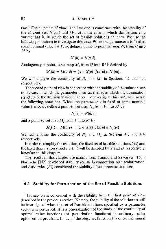
94 4 STABILITY
two different points of view. The first one is concerned with the stability ofthe efficient sets N(u, v) and M(u, v) in the case in which the parameter uvaries; that is, in which the set of feasible solutions changes. We use thefollowing notations to investigate this case. When the parameter v is fixed atsome nominal value vE V, we define a point-to-point set map N1 from U intoWby
N1(u) = N(u, v).
Analogously, a point-to-set map M1 from U into W is defined by
M1(u) = M(u, v) = {x E X(u) :f(x, u) E N1(u)}.
We will analyze the continuity of N1 and M1 in Sections 4.2 and 4.4,respectively.
The second point of view is concerned with the stability of the solution setsin the case in which the parameter v varies; that is, in which the dominationstructure of the decision maker changes. To investigate this case, we also usethe following notations. When the parameter u is fixed at some nominalvalue U E U, we define a point-to-set map N2 from V into RP by
N2(v) = N(u, v)
and a point-to-set map M2 from V into R" by
M2(v) = M(u, v) = {x E X(u) :f(x, u) E Niv)}.
We will analyze the continuity of N2 and M2 in Sections 4.3 and 4.4,respectively.
In order to simplify the notation, the fixed set of feasible solutions Y(u) andthe fixed domination structure D(v) will be denoted by Y and D, respectively,hereafter in this chapter.
The results in this chapter are mainly from Tanino and Sawaragi [TlO].Naccache [N2] developed stability results in connection with scalarization,and Jurkiewicz [13] considered the stability of compromise solutions.
4.2 Stability for Perturbation of the Set of Feasible Solutions
This section is concerned with the stability from the first point of viewdescribed in the previous section. Namely, the stability of the solution set willbe investigated when the set of feasible solutions specified by a parametervector u is perturbed. It is a generalization of the study of the continuity ofoptimal value functions (or perturbation functions) in ordinary scalaroptimization problems. In fact, if the objective function f is one-dimensional

4.2 STABILITY FOR PERTURBATION OF FEASIBLE SOLUTIONS 95
(scalar-valued), then the map N1 is at most single-valued and so might beidentified with the optimal value function
w(u) ,= inf{f(x, u): x E X(u)}.
The continuity, especially lower semicontinuity, of this function is closelyrelated to the duality in scalar optimization.
In this section the domination structure is fixed and so is considered to bea point-to-set map from
y(U) ,= u y(u)UE U
into RP. Moreover, the point-to-set map int D, which is defined by
(int D)(y) =. int D(y) u {OJ for every y,
is considered to provide another domination structure.
4.2.1 Upper Semicontinuity of the Map N,
First, we consider sufficient conditions for the upper semicontinuity of themap N1 • The following lemma is useful in this chapter.
Lemma 4.2.1
Let Q be a point-to-set map from a set Y into RP. Suppose that Q is lowersemicontinuous at y E Y and that Q(y) is convex for every y E Y near y. Let{yk} c Yand {z"} c RP be sequences that converge to y and Z, respectively,and suppose that Z E int Q(Y). Then Zk E Q(yk) except for a finite number ofk's.
Proof We denote the closed unit ball in RP by B. As Z E int Q(y), thereexists a positive real number J such that z+ JB c Q(Y). Since z" -+ Z, there isa number m such that
Zk E Z + int (c5j2)B for all k ~ m.
Let k ~ m, and suppose that Zk ¢ Q(yk). Here we may assume that Q(yk) is aconvex set, since Q(y) is convex for any y near y. Then the separation theoremof convex sets (Theorem 2.1.1) guarantees the existence of a vector A E R!such that II AII = 1 and
Q(yk) c {z E RP: (A, z) ~ 0, z")}.

96
Then the vector
4 STABILITY
Zk = Z + (b12 + (2,i' - z»"lsatisfies
In fact,
Zk E =+ int bB and Zk ¢ 0(1) + int(b/2)B.
and
Ilzk - =11 = 1"/2 + (2,Zk - =)III"l11 ~ "/2 + 1(2, i' - =)1
~ fJ/2 + 11"l1111i' - =11 < fJ/2 + "/2 = fJ
(2, Zk) = (2, z) + bl2 + (2,Zk - =) = fJI2 + (2, i');
whence, for any Z E 0(1),
IIzk - z] ~ 1(2,zk - z)1 = 1(2,zk) - ("l,i'») + (2,i') - (2,z»)1 ~ b12.
Thus, if we assume that Zk ¢ OV) for an infinite number of k's, then we cantake an infinite number of Zk satisfying the above properties. The set of thosepoints Zk has a cluster point in the compact set z+ fJB, which is denoted by Z.By taking a subsequence if necessary, we may assume without loss ofgenerality that zk exists for every k ~ m and Zk --+ Z. Since z E Z + fJB c O(y)and 0 is lower semicontinuous at y, there exist a number m' and a sequence{Zk} such that Zk E 0(1) for k ~ m' and Zk --+ Z. Then Zk - Zk --+ O. This,however, contradicts the fact that
Zk ¢ 0(/) + int(fJI2)B.
Therefore, the number of k's for which Zk ¢ 0(1') is finite. This completes theproof.
The following theorem provides sufficient conditions under which the mapN 1 is upper semicontinuous.
Theorem 4.2.1
The map N 1 is upper semicontinuous at UE U if the following conditionsare satisfied:
(i) the map Y is continuous at u;(ii) the map D is lower semicontinuous on Y(u);
(iii) D(y) is a convex set for every yES n Y(u), with U E T, where Sand Tare some neighborhoods of Y(u) and U, respectively;
(iv) the relationship N1(u) = 8(Y(u), int D) holds.
Proof Let
{Uk} c U, Uk --+ U, I' EN1(Uk), and I' --+ y.
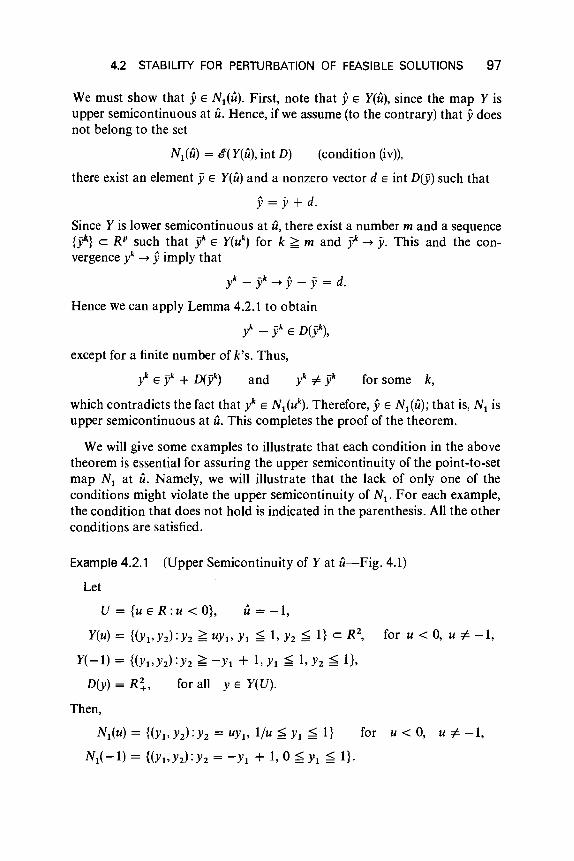
4.2 STABILITY FOR PERTURBATION OF FEASIBLE SOLUTIONS 97
We must show that y E Nt(U). First, note that yE Y(u), since the map Y isupper semicontinuous at U. Hence, if we assume (to the contrary) that ydoesnot belong to the set
Nt(u) = &'(Y(u), int D) (condition (ivj),
there exist an element y E Y(u) and a nonzero vector d E int D(y) such that
y = y + d.
Since Y is lower semicontinuous at U, there exist a number m and a sequence{?} c RP such that t E Y(uk
) for k ;;::; m and t -+ y. This and the con-vergence l -+ Yimply that
l - yk -+ Y- y = d.
Hence we can apply Lemma 4.2.1 to obtain
l- t E D(t),
except for a finite number of k's. Thus,
l E yk + D(yk) and l i' t for some k,
which contradicts the fact that l E Nt(u k) . Therefore, y E Nt(u); that is, N, is
upper semicontinuous at U. This completes the proof of the theorem.
We will give some examples to illustrate that each condition in the abovetheorem is essential for assuring the upper semicontinuity of the point-to-setmap Nt at U. Namely, we will illustrate that the lack of only one of theconditions might violate the upper semicontinuity of Nt. For each example,the condition that does not hold is indicated in the parenthesis. All the otherconditions are satisfied.
Example 4.2.1 (Upper Semicontinuity of Y at u-Fig. 4.1)
Let
U = {u E R: u < O}, U= -1,
Y(u) = {(Yt'Y2) :Y2 ;;::; uYt, Yt ~ 1, Y2 ~ I} C R 2, for u < 0, u i' -1,
Y(-l) = {(Yt'Y2):Y2;;::; -Yt + 1,Yt ~ l'Y2 ~ I},
D(y) = R~, for all Y E Y(U).
Then,
Nt(u) = {(Yt'Y2):Y2 = uYt, l/u ~ Yt ~ I} for u < 0, u i' -1,
Nt( -1) = {(Yl'Y2) :Y2 = -Yt + 1, 0 ~ Yt ~ I}.
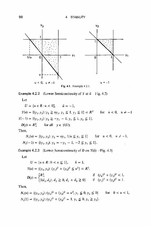
98 4 STABILITY
-......!....--*-,...--:.-....:.....t--- Yl
u < 0, U ~ -1
-----l-------..::Ik--- Yl
U = -1Fig. 4.1. Example 4.2.1.
Example 4.2.2 (Lower Semicontinuity of Y at u-Fig. 4.2)
Let
U = {u E R: u.«: OJ, U= -1,
Y(U)={(Yl'Y2):Y2~UYl'Yl~1'Y2~1}cR2 for u<O, uof--1
Y(-1) = {(Yl'Y2): Y2 ~ -Yl - 1, Yl ~ 1,Y2 ~ 1},
D(y) = R~ for all Y E Y(U).
Then,
N1(u) = {(Yl'Y2):Y2 = UYl' 1/u ~ Yl ~ 1} for U < 0, U of- -1,
N1(-l) = {(Yl'Y2):Y2 = -Yl - 1, -2 ~ Yt ~ 1}.
Example 4.2.3 (Lower Semicontinuity of Don y(u)-Fig. 4.3)
Let
if (Yt)2 + (Y2)2 < 1,
if (y1f + (Y2)2 = 1.
Then,
N1(u) = {(Yt,Y2): (Ytf + (Y2)2 = u2,Yl ~ 0, Y2 ~ O} for °< u < 1,
N1(1) = {(Yl'Y2): (Yl)2 + (Y2)2 = 1, Yl ~ 0, Yl ~ Y2}'
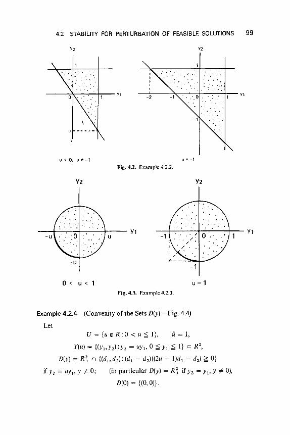
4.2 STABILITY FOR PERTURBATION OF FEASIBLE SOLUTIONS 99
, . ; .. ' ..;' .
. . . '.'
yz
. '.. . "".-2
u < 0, u"-1 U = -1
Fig. 4.2. Example 4.2.2.
Y2 Y2
-1III .
~~-~~._..--1
--t----t----+-- Ylu
-u
-u---t---;--;----:------Ir--- Y1
o < u < u = 1
Fig.4.3. Example 4.2.3.
Example 4.2.4 (Convexity of the Sets D(y)-Fig. 4.4)
LetU = {u E R: 0 < U ~ 1}, U= 1,
Y(u) = {(Yl,h):Yz = UY1' 0 ~Yl ~ 1} c RZ,
D(y) = R~ n {(d1, dz) : (d1 - dz)«2u - l)d 1 - dz) ~ O}
if Yz = UY1' Y =1= 0; (in particular D(y) = R~ if Yz = Yl' Y =1= 0),
D(O) = {(O, on.
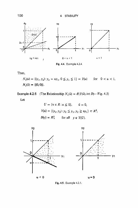
100 4 STABILITY
Y2 Y2
o_-¥- --I.__ VI
o-~---~-V,
. ' .. '.1 '-'-':_'-'---. ,
',", ",O(V)'
V2 = UVI 0< U < 1 U = 1
Fig. 4.4. Example 4,2.4,
Then,
N1(u) = {(Yl'YZ):Yz = UY1' 0 ~Yl ~ 1} = Y(U)
N1(1) = {(O,On.
for 0 < U < 1,
Example 4.2,5 (The Relationship N1(U) = 0"(Y(u), int D)-Fig. 4.5)
Let
u = {u E R: U ~ O}, U = 0,
Y(u) = {(Yl'Y2);Y2 ~ Yl' Y2 ~ uyd c RZ,
D(y) = R~ for all y E Y(U).
Y2 Y2
_....:::::::~---:._....:....J- Y1 _-j,'--__---L Yl
u < 0 u=o
Fig. 4.5. Example 4,2,5,
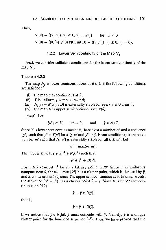
4.2 STABILITY FOR PERTURBATION OF FEASIBLE SOLUTIONS 101
Then,
Nl(u) = {(Yl,Yz):Yl ~ 0, Y2 = UYl} foru < 0,
Nl(O) = {(O,O)} =f. <ff(Y(O), int D) = {(Yl'Y2):Yl ~ 0, Y2 = O}.
4.2.2 Lower Semicontinuity of the Map N,
Next, we consider sufficient conditions for the lower semicontinuity of themapNl·
Theorem 4.2.2
The map N, is lower semicontinuous at Ii E U if the following conditionsare satisfied: .
(i) the map Yis continuous at Ii;(ii) Y is uniformly compact near Ii;
(iii) Nl(u) = t!(Y(u), D) is externally stable for every u E U near Ii;(iv) the map D is upper semicontinuous on Y(Ii).
Proof Let
and
Since Yis lower semicontinuous at Ii, there exist a number m' and a sequence{Y'} such that Y' E Y(u~ for k ~ m' and Y' -+ y. From condition (iii),there is anumber mil such that Nl(Uk
) is externally stable for all k ~ mil. Let
m = max(m', mil).
Then, for k ~ m, there is jik E Nl(Uk) such that
Y' E t + D(jik).
For 1 ;;; k < m, let 1 be an arbitrary point in RP. Since Y is uniformlycompact near Ii, the sequence {t} has a cluster point, which is denoted by ji,and is contained in Y(Ii) since Yis upper semicontinuous at Ii. In other words,the sequence {Y' - jik} has a cluster point y - ji. Since D is upper semicon-tinuous on Y(Ii),
y - ji E D(ji);
that is,
YE ji + D(ji).
If we notice that y E Nl(Ii), ji must coincide with y. Namely, y is a uniquecluster point for the bounded sequence {t}. Thus, we have proved that the
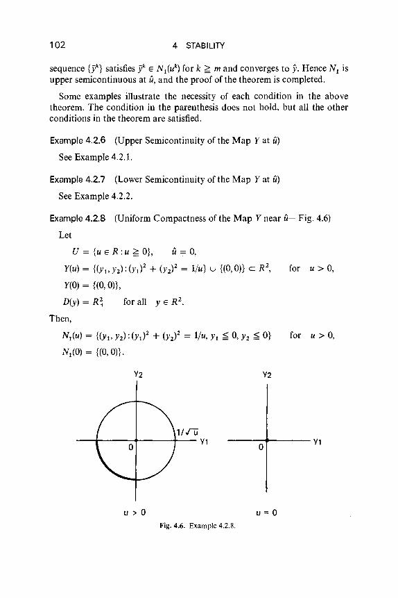
102 4 STABILITY
sequence Ui} satisfies Si E N1(Uk) for k ~ m and converges to y. Hence N1 isupper semicontinuous at u, and the proof of the theorem is completed.
Some examples illustrate the necessity of each condition in the abovetheorem. The condition in the parenthesis does not hold, but all the otherconditions in the theorem are satisfied.
Example 4.2.6 (Upper Semicontinuity of the Map Yat u)
See Example 4.2.1.
Example 4.2.7 (Lower Semicontinuity of the Map Yat u)
See Example 4.2.2.
Example 4.2.8 (Uniform Compactness of the Map Y near u-Fig. 4.6)
Let
U = {u E R: U ~ O}, U = 0,
Y(u) = {(Yl' Y2): (Yl)2 + (Y2)2 = l/u} u {(O,O)} C R2,
Y(O) = {(O,O)},
D(y) = R~ for all Y E R 2•
Then,
Nt(u) = {(Yt, Y2): (Yt)2 + (Y2f = l/u, Yt ~ 0, Y2 ~ O}
Nt (0) = {(O, O)}.
for u > 0,
for u > 0,
Y2
o---.......----Y11/1U
----t----+-----I-- Y1
u > 0 u=oFig. 4.6. Example 4.2.8.
4.2 STABILITY FOR PERTURBATION OF FEASIBLE SOLUTIONS 103
Y2
/<'"":' :' .....,.. '. '. . :-. . \"' , \" . ". ' ,
-u"'~:O,"'.'··,\. '.. ' I". ". I, .. . . "/
<; -:>
-u
u > 0
Y2
- .............:..----1-..:~-r+-- Yl-1
-1
u=O
Fig. 4.7. Example 4.2.9.
Example 4.2.9 (External Stability of N1(u), Compactness of the Set Y(u)-Fig. 4.7)
Let
u = {u E R: u > a}, ii = 1,
Y(u) = {(Yl' Yz): (Yl)2 + (Yz)2 < u2} C R2
Y(l) = {(Yl' Y2): (YI)2 + (Yz)2 ~ 1},
D(y) = R~ for all Y E R 2•
Then
for u > 0, u i= 1,
N1(u) = 0 for u > 0, u i= 1,
N1(1) = {(Yl' Yz): (Yl)2 + (Yz)2 = 1, Yl ~ 0, Yz ~ a}.
Example 4.2.10 (External Stability of N 1(u), Upper Semicontinuity of D onY(u)-Fig.4.8)
Let
U = {u = lin: n is a positive integer} u {a}, Ii = 0,
Y(u) = {(Yl' Yz):°~ Yl ~ 1, Y2 = u} C R2,
{
{(dl ' d2) :°~ d1 ~ kin - YI} for (k - l)ln < Yl ~ kin,
D(y) = k = 1, ... ,n, Y2 = lin,
{(d1,d2):d l = O} for YI = ° or Y2 = 0.

104 4 STABILITY
kin - Y,
o--+-----dl
1/no---f---,,.,...------- dl
.'.
(k - 1)/n < Yl ~ kin, Y2 = 1/n
Y2
Yl = 0 or Y2 = 0
Y2
1/n..-----....,
o-+------Ylo
--t-------J.- Yl
u = 1/n u=oFig. 4.8. Example 4.2.10.
Then,N1(u) = {(O, un for u = lin,
N1(0) = {(Yl'Yz): 0 s Yl ~ 1, Yz = O}.
Example 4.2.11 (External Stability of N 1(u), Asymmetry of D- Fig 4.9)
LetU = {u E R: u !?; O}, U = 0,
Y(u) = {(Yl'YZ):O ~ Yl ~ 1, 0 ~ Yz ~ uyd c RZ;
in particular, Y(O) = {(Yl' Yz): 0 ~ Yl ~ 1, Yz = O},
D(y) = {(d1, dz) :d1 = O} for all Y E Y(U).
Then,
N1(u) = {(O, On for u > 0,
N1(0) = {(Yl' Yz): 0 ~ Yl s 1, Yz = O}.

4.2 STABILITY FOR PERTURBATION OF FEASIBLE SOLUTIONS 105
Y2 Y2
1o-+------- Y1o
u > 0 u=oFig. 4.9. Example 4.2.11.
Example 4.2.12 (External Stability of N 1(u), Transitivity of D-Fig. 4.10)
Let
U = {u E R :°~ u ~ f}, u= 0,
Y(u) = {(Yl Y2): u ~ Yl ~ 1, Y2 = O},u {(Yl'Y2): u ~ Yl ~ 1, Yl = Y2}
{
{(d1' d2) :d1 = 0, d2 ~ O} if Y2 = 0, Yl #- 0,
D(y) = {(d1,d2): d2 = 2d1 ~ O} if Yl = Y2 #- 0,
{(d1,d2): d1 ~ 0, d2 ~ 2dd if Y = (0,0).
Then,
N1(u) = {(Yl'Y2):f < Yl ~ 1, Y2 = O} for °< u ~ t,N1(0) = {(O, On u {(Yl'Y2):f < Yl ~ 1, Y2 = O}.
Example 4.2.13 (Upper Semicontinuity of the Map Don y(u)-Fig. 4.11)
Let
U = {u E R: u ~ O}, U= 0,
Y(u) = {(Yl'Y2): 0 ~ Yl ~ 1, UYI s Y2 s I} C R 2,
{
{(dl' d2): d1 ~ 0, d2 ~ udd if Y2 = UYl'Y#-O for U > 0,
D(y) = {(d1,d2): d1 = 0, d2 ~ O} if Yl = 0, Y2 #- 0,
{(d1,d2): d1 ?; 0, d2 > O} if Y2 = 0.
Then,
N1(u) = {(O,O)} for u > 0,
N1(0) = {(Yl'Y2): 0 ~ Yl ~ 1,Y2 = O}.
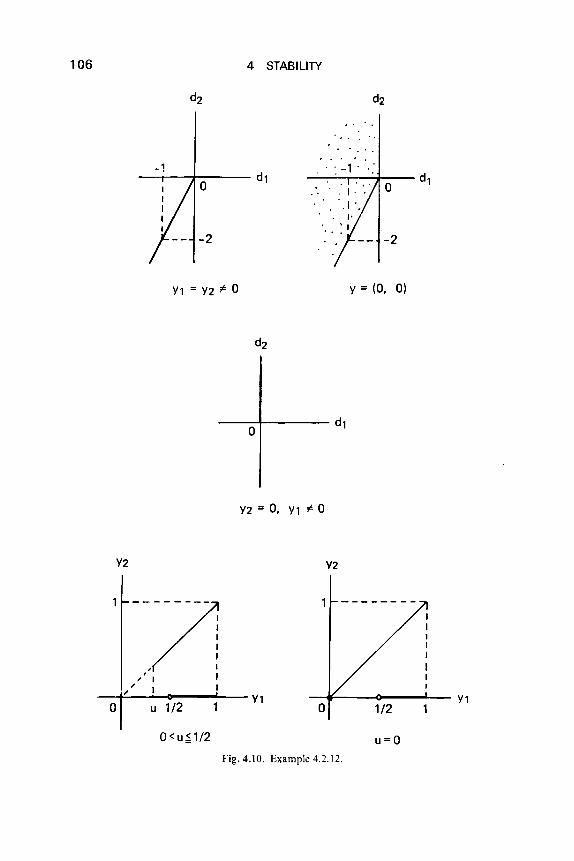
106 4 STABILITY
-. . '.
-1
o
. ... " -1 . ':
o
-2
Y1 = Y2 ~ 0 Y = (0, 0)
o-----t----- d1
Y2 = 0, Y1 'i' 0
Y2 Y2
--¥--_-o-__..L-_ Y1~~__cI,....- .....-- Y1o 1/2
u=oFig. 4.10, Example 4.2.12.
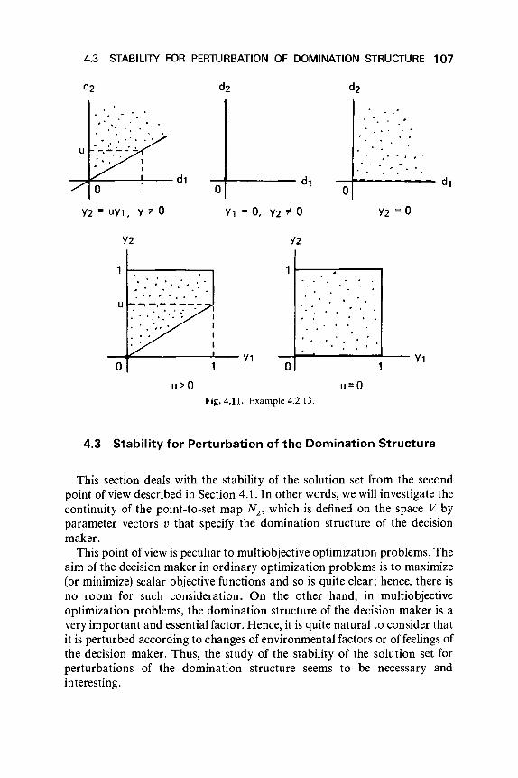
4.3 STABILITY FOR PERTURBATION OF DOMINATION STRUCTURE 107
.. ' ... .. , ,;
1o-1------......-- Ylo
_....-=:~ ---L__ Yl
u>O u=OFig. 4.11. Example 4.2.13.
4.3 Stability for Perturbation of the Domination Structure
This section deals with the stability of the solution set from the secondpoint of view described in Section 4.1. In other words, we will investigate thecontinuity of the point-to-set map Nz, which is defined on the space V byparameter vectors v that specify the domination structure of the decisionmaker.
This point of viewis peculiar to multiobjective optimization problems. Theaim of the decision maker in ordinary optimization problems is to maximize(or minimize) scalar objective functions and so is quite clear; hence, there isno room for such consideration. On the other hand, in multiobjectiveoptimization problems, the domination structure of the decision maker is avery important and essential factor. Hence, it is quite natural to consider thatit is perturbed according to changes of environmental factors or of feelings ofthe decision maker. Thus, the study of the stability of the solution set forperturbations of the domination structure seems to be necessary andinteresting.
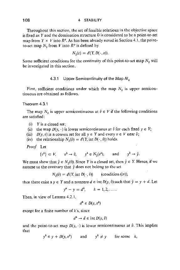
108 4 STABILITY
Throughout this section, the set of feasible solutions in the objective spaceis fixed as Y and the domination structure D is considered to be a point-to-setmap from Y x V into RP. As has been already noted in Section 4.1, the point-to-set map Nz from V into RP is defined by
Niv) = 6'(Y, D(·, v)).
Some sufficient conditions for the continuity of this point-to-set map Nz willbe investigated in this section.
4.3.1 Upper Semicontinuity of the Map N 2
First, sufficient conditions under which the map Nz is upper semicon-tinuous are obtained as follows.
Theorem 4.3.1
The map N z is upper semicontinuous at vE V if the following conditionsare satisfied:
(i) Y is a closed set;(ii) the map D(y, . ) is lower semicontinuous at v for each fixed y E Y;
(iii) D(y, v) is a convex set for all y E Y and every v E V near v;(iv) the relationship Nz(v) = 6'(Y, int D(·, v)) holds.
Proof Let
and
We must show that y E Nz(v). Since Y is a closed set, then y E Y. Hence, if weassume to the contrary that ydoes not belong to the set
Niv) = 6'(Y, int D(·, v)) (condition (iv)),
then there exist aYE Y and a nonzero d e int D(y, v) such that y = y + d. Let
Y' - y = d",
Then, in view of Lemma 4.2.1,
k = 1,2, ....
dk E D(y, Vk)
except for a finite number of k's, since
dk --+ d E int D(y, v)
and the point-to-set map D(y, . ) is lower semicontinuous at v. This impliesthat
and for some k,

4.3 STABILITY FOR PERTURBATION OF DOMINATION STRUCTURE 109
-v
V2
-+---'---.j-"'----+- Vt
-1
v > 0
Fig. 4.12. Example 4.3.1.
V2
-1
v=O
which contradicts the assumption yk E Nitf). Therefore ymust be containedin N2(v). Namely, N2 is upper semicontinuous at v and the proof iscompleted.
Some examples are given in the following to illustrate the necessity of eachcondition in the theorem.
Example 4.3.1 (Closedness of the Set Y-Fig. 4.12)
Let
v = {v E R: v ~ O}, v=0,
Then,
for all Y E Y.
N2(v) = {(Yl'Y2): (Yl)2 + (Y2)2 = 1, Yl ~ 0, Y2 ~ vy,}
N2(0) = {(Yl'Y2): (Yl)2 + (Y2)2 = 1, Yl ~ 0,Y2 < O}.
for v> 0,
Example 4.3.2 (Lower Semicontinuity of the Map D(y, .) at v-Fig. 4.13)
Let
v = {v E R: v > O}, v= 1,
Y = {(Yl,Y2): (Yl)2 + (Y2)2 ~ 11} C R2,
D(y, v) = R~ for all Y E Y if v > 0, v ¥- 1,
for all y.'

110 4 STABILITY
Y2 V2
-1o
D
~.-.-: 1 .
-1--'---~-- dl
v = 1 v > 0, v F 1
Fig. 4.13. Example 4.3.2.
v =1
Then,
Nz(v) = {(Yl'YZ): (Yl)Z + (YZ)Z = 1, Yl ~ 0, Yz ~ O}
for v > 0, v ¥= 1,
Nz{l) = {(Yl' Yz): (Yl)Z + (Yz)Z = 1, Yl ~ 0, Yz ~ Yl}'
Example 4.3.3 (Convexity of the Set D(y, v)-Fig. 4.14)
Let
V={vER:O<v~l}, fJ=l,
Y = {(Yl'YZ): 0 ~ Yl ~ 1, Yl = Yz} c RZ,
D(y, v) = {(d1 , dz): d, ~ 0, dz ~ 0,
(d1 - (2v - l)dz)((2v - l)d l - dz) ~ O} for all Y E Y.
In particular,
D(y, 1) = R~ for all Y E Y.
Then,
Nz(v) = {(Yl'YZ): 0 ~ YI ~ 1, YI = Yz}
Nz(l) = {(O,O)}.
for 0 < v < 1,
Example 4.3.4 (The Relationship Nz(fJ) = &'(Y, int D(·, v))-Fig. 4.15)
Let
v = {v E R: v ~ O}, v = 0,
Y = {(YI'YZ): -YI + Yz ~ 0, Yz ~ O} c RZ,
D(y, v) = {(d 1, dz) : -vdt + dz ~ 0, d, + vdz ~ O} for all Y E Y,
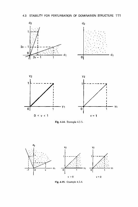
4.3 STABILITY FOR PERTURBATION OF DOMINATION STRUCTURE 111
o--+------- dl
. , .. . . .
. . ,
. . . .
Y2 Y2
o_-+ L-_ Yl
o---f&--------O'-- Yl
o < v < 1 v = 1
Fig. 4.14. Example 4.3.3.
Y2
1 -----.1 •
·1.· ..,'I ",. ''''''.. '.:. ".. '
o
Y2
1 ----- .
-1f-----"-- YIo
v > 0 v=o
Fig. 4.15. Example 4.3.4.
112
In particular,
4 STABILITY
Then,
D(y,O) = R~ for all y E Y.
Niv) = {(Yt, Y2): Yt ~ 0, Y2 = O}
N2(0) = {(O, On # tC(Y, int D(·, 0))
= {(Yl' Y2): Yt ~ 0, Y2 = OJ.
for v> 0,
4.3.2 Lower Semicontinuity of the Map N 2
The fourth theorem in this chapter provides sufficient conditions for thelower semicontinuity of the map N2 •
Theorem 4.3.2
The map N2 is lower semicontinuous at vE V if the following conditionsare satisfied:
(i) Y is a compact set;(ii) N2(v) = tC(Y, D(·, v)) is externally stablefor every v near v;(iii) D is upper semicontinuous on Y x V.
Proof If Yis empty, the theorem is obviously true. So we assume that Yisnon empty . Let
{vk} c: V, vk ~ v, and y E Niv).
From condition (ii), there exist a number m and l E N2(Vk
) for k ~ m suchthat
YE l + D(l, vk) .
Let l be an arbitrary point in Yfor 1 ~ k < m. Since Yis a compact set, thesequence {l} has a cluster point in Y, which is denoted by y. In other words,the sequence {y -l} has a cluster point y - y. Since
y - l E D(yk, vk) for k ~ m
and D is upper semicontinuous on Y x v,y - Y E D(y, v).
By combining this with the fact y E N2(v), we have y = y. Namely, y is aunique cluster point for the bounded sequence {l}. Thus, we have provedthat the sequence {l} satisfies
l E N2(if) for k ~ m and l ~ y.

4.3 STAB/LIlY FOR PERTURBATION OF DOMINATION STRUCTURE 113
--~---1----- Y1-1 a
-1
Fig.4.16. Example 4.3.5.
Therefore, the map N2 is lower semicontinuous at vand the proof of thetheorem is completed.
Some examples are given in the following.
Example 4.3.5 (Closedness of the Set Y-Fig. 4.16)
Let
v = {v E R: v ~ O}, v= 0,
Y = {(Yl,Y2):Yl + Y2 = -1, -1 < Yl ;:;; O} u {(O,O)} C R 2,
for all Y E Y.
Then,
for v> 0,
Example 4.3.6 (Boundedness of the Set Y-Fig.4.17)
In Example 4.3.5, we replace Y by a new set defined by
Then,
for v> 0,

114 4 STABILITY
.1 '.' ". I ' .
. .: ,', D(vl,. '. ',I " '. .. '.
-1 0-------+--- Yl
Fig. 4.17. Example 4.3.6.
Example 4.3.7 (External Stability of N2(v), Upper Semicontinuity of D(·, v)on Y for v near v-Fig. 4.18)
for (k - l)ln < y ~ kin,
k = 1",., n,
for y = 0
Let
v = {v = lin: n is a positive integer} u {O},
Y = {y: 0 ~ y ~ I} c R,
{
{d :0 ~ d s kin - y}
D(y, v) =
{O}
v = 0,
if v = lin.
Then,
N2(v) = {O}, for v = lin,
N2(O) = {y: 0 ~ y ~ 1}.
-----------+) Y
kin - y) d, , -'d • )d •
0 lin 0 0
(k - 1lin < y ~ kin y=O O&y~l
if v = lin if v=O
• I ) Y0 0
v = lin v=OFig. 4.18, Example 4.3.7.

4.3 STABILITY FOR PERTURBATION OF DOMINATION STRUCTURE 115
........ 0---.---t--- d1
o----f.---- d1
v < Y1 s 1 o ~ Y1 ~ v
Y2 Y2
1 -------
o--1J------.........- Y1
o--+-------'-- Y1
O<v<1 v=O
Fig. 4.19. Example 4.3.8.
Example 4.3.8 (External Stability ofN 2(V),Asymmetry ofD(., v)-Fig.4.19)
Let
v = {v E R : 0 ~ v < 1}, iJ = 0,
y = {(Yl'Y2):O ~ Yl ~ 1, Yz = O}
u {(Yl'YZ):O~Yl ~ 1'Yl =yz},
{
{(d1, dz) : d1 = O} if v < Yl ~ 1,D(y, v) =
{(d1, dz) :d1 ~ O} if 0 ~ Yl ~ V.
Then,
Nz(v) = 0 for 0 < v < 1,
Nz(O) = {(O, On.
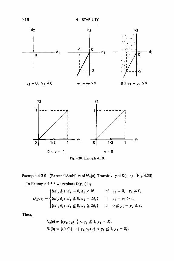
116 4 STABILITY
o
-2
. -1 '. .-----.----1--- dl
o--J----- d l
Y2 = 0, Yl "# 0 Yl = Y2 > v o ~ Yl = Y2 ~ v
Y2 Y2
1/2a-#f------<_-...L- Yl
1/2a_~-~_-...L- Yl
o < v < v=O
Fig. 4.20. Example 4.3.9.
if Yl = Y2 > v,
if Y2 = 0, Yl i: 0,
if 0 ~ Yl = Y2 s V.
Example 4.3.9 (External Stability ofN iv), Transitivity ofD(·, v)-Fig. 4.20)
In Example 4.3.8 we replace D(y, v) by
{
{(dl ' d2 ) : dl = 0, d2 ~ O}
D(y, v) = {(dl' d2 ) ; d t ~ 0, d2 = 2dt }
{(dl' d2 ) : dl ~ 0, d2 ~ 2dt }
Then,
N2(v) = {(Yl'Y2):! < Yt ~ l'Y2 = a},
N2(O) = {(O,O)} U {(Yl,h):! <v. ~ l'Y2 = O}.

4.3 STABILITY FOR PERTURBATION OF DOMINATION STRUCTURE 117
v > 0, v t- 1
-1
-1
v = 1
Fig. 4.21. Example 4.3.10.
Example 4.3.10 (Upper Semicontinuity of the Map D(y, .) at v-Fig. 4.21)
Let
v = {v E R: v> O}, v= 1,
Y = {(YI'Yz): (YI)Z + (Yz)Z ~ 1} c RZ,
D(y, v) = {(d l , dz) : dz ~ 0, d l + dz ~ o}
for all Y E Y if v > 0, v # 1,
D(y, 1) = R~ for all Y E Y.
Then,
Nz(v) = {(YI' Yz): (Yt)Z + (yzf = 1, YI ~ 0, YI - Yz ~ O}
for v > 0, v # 1,
Nz(1) = {(YI'Yz): (YI)Z + (Yz)Z = 1, YI ~ 0, Yz ~ O}.
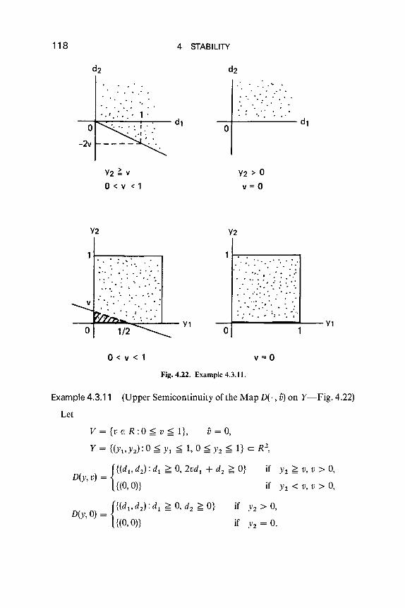
118
o-2v
. " .. , . ' .• • s • : • ~. 1,
Y2 ~ v
o < v < 1
4 STABILITY
d2
..:
.'d1
0d1
Y2 > 0v=o
Y2
.. . .. .'.::". ... '~ ...:"".: ".:' ".. ". 0..... .. ~ ...." " .. ".- ..
0< v < 1
Y2
1 .'. '. .' 0. . ~ .
. ... . ..' ... ...... " .. :. "; . ': . ", ,--1-----......-- Y1o
v=O
Fig. 4.22. Example 4.3.11.
Example 4.3.11 (Upper Semicontinuity of the Map D(·, f;) on Y-Fig.4.22)
Let
v = {v E R : 0 ~ v ~ 1}, f; = 0,
Y = {(Yl'YZ):O ~ Yl ~ 1, 0 ~ Yz ~ 1} c RZ,
if Y2 ~ D, V > 0,
if Y2 < v, D > 0,
if Y2 > 0,
if Y2 = O.
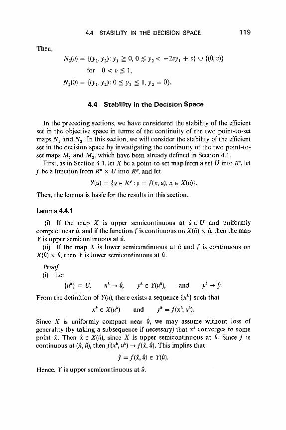
Then,
4.4 STABILITY IN THE DECISION SPACE
Nz(v) = {(Yt,Yz): Yt ~ 0, °;<£ Yz < -2vYt + v} u {CO, v)}
for 0 < v ;<£ 1,
Nz(O) = {(Y\,Yz): °;<£ Y\ ;<£ 1, Yz = OJ.
4.4 Stability in the Decision Space
119
In the preceding sections, we have considered the stability of the efficientset in the objective space in terms of the continuity of the two point-to-setmaps N, and Nz . In this section, we will consider the stability of the efficientset in the decision space by investigating the continuity of the two point-to-set maps M\ and M z, which have been already defined in Section 4.1.
First, as in Section 4.1, let X be a point-to-set map from a set U into R", letf be a function from R" x U into RP, and let
Y(u) = {y E RP: Y = f(x, u), X E X(u)}.
Then, the lemma is basic for the results in this section.
Lemma 4.4.1
(i) If the map X is upper semicontinuous at UE U and uniformlycompact near U, and if the function f is continuous on X(u) x U, then the mapYis upper semicontinuous at ii.
(ii) If the map X is lower semicontinuous at uand f is continuous onXCii) x ii, then Y is lower semicontinuous at U.
Proof(i) Let
{Uk} c U, Uk -+ u, yk E Y(uk), and yk -+ y.
From the definition of Y(u), there exists a sequence {x k} such that
x k E X(u k) and yk = f(x k, Uk).
Since X is uniformly compact near ii, we may assume without loss ofgenerality (by taking a subsequence if necessary) that x k converges to somepoint x. Then xE XCii), since X is upper semicontinuous at u. Since f iscontinuous at (x, ii), then f(xk
, Uk) -+ f(x, u). This implies that
y = f(x, ii) E y(u).
Hence, Y is upper semicontinuous at U.

120
(ii) Let
4 STABILITY
{Uk} C V, Uk -+ u, and y E y(u).
From the definition of Y(u), there exists x E X(u) such that y = f(x, u). SinceX is lower semicontinuous at U, there exist a number m and a sequence {x'}such that
x k E X(u k) for k ~ m
If we let yk = f(x k, Uk), then
yk E Y(uk) for k ~ m and
in view of the continuity off. Thus we have obtained that yk -+ y, whence Y islower semicontinuous at U. This completes the proof of the lemma.
Next, in addition to X and f, let N be a point-to-set map from V into RPsuch that N(u) c Y(u), and let
M(u) = {x E X(u) :f(x, u) E N(u)}.
Then, we get the following lemma, which is also fundamental in this section.This lemma provides the relationships between the continuity of point-to-setmaps in the decision and objective spaces.
Lemma 4.4.2
(i) If X is upper semicontinuous at U, if N is upper semicontinuous at Ii,and iff is continuous at X(Ii) x U, then the map M is upper semicontinuousat Ii.
(ii) If X is upper semicontinuous at uand uniformly compact near Ii, if Nis lower semicontinuous at Ii, and if f is continuous and' one-to-one onX(Ii) x U, then M is lower semicontinuous at U.
Proof(i) Let
and
Since X is upper semicontinuous at U, x E X(u). From the definition of M(u),f(x k
, Uk) E N(u k) . From the continuity off,
f(xk, Uk) -+ f(x, u).
Hence, f(x, Ii) E N(u), since the map N is upper semicontinuous at U.Therefore, xE M(U), and so the map M is upper semicontinuous at U.
(ii) Let
and XE M(u).
4.4 STABILITY IN THE DECISION SPACE 121
From the definition of M(u), f(x, U) E N(u). Since N is lower semicontinuousat uand N(u) c Y(u), there exist a number m and a sequence {xk
} such that
x k E M(uk) for k ~ m and f(xk
, Uk) --+ f(x, U).
Since X is uniformly compact near U, the sequence {x k} has a cluster point x.
Since X is upper semicontinuous at U, x E X(U). Then, sincef is continuous,
f(x, U) = f(x, u),
and so we have x = X, since f(', u) is one-to-one on X(u); that is, xis a uniquecluster point of the bounded sequence {x"}. This implies that xk --+ x, andtherefore M is lower semicontinuous at U. This completes the proof of thelemma.
We can combine these lemmas and the theorems obtained in Sections 4.2and 4.3 to yield a series of theorems as follows.
First, with regard to the continuity of the point-to-set map MI , thefollowing theorems are obtained. (Notice the fact that Y is uniformlycompact near u if X is so, and f is continuous on cl UueT X(u) x T alongwith some compact neighborhood Tin U of u.)
Theorem 4.4.1
The map MI is upper semicontinuous at uE U under the followingconditions:
(i) the map X is continuous at u;(ii) X is uniformly compact near u;
(iii) f is continuous on X(u) x u;(iv) the map D is lower semicontinuous on Y(u);(v) D(y) is a convex set for every yES (\ Y(u) with u E T, where Sand T
are some neighborhoods of Y(u) and U, respectively; and(vi) NI (u) = $(Y(u), int D).
Theorem 4.4.2
The map MI is lower semicontinuous at uE U under the followingconditions:
(i) the map X is continuous at u;(ii) X is uniformly compact near u;
(iii) f is continuous on cl UueT X(u) x T with a compact neighborhoodTin U of u and one-to-one on X(u) x u;
(iv) NI(u) is externally stable for every u E U near u; and(v) the map D is upper semicontinuous on Y(u).

122 4 STABILITY
Next, in order to consider the continuity of the point-to-set map M 2 , weassume for simplicity that the set of feasible solutions is X and that thevector-valued objective function from X into RP is f(x). The followingtheorems are readily obtained from Theorems 4.3.1 and 4.3.2, respectively.
Theorem 4.4.3
The map M2 is upper semicontinuous at vE V under the followingconditions:
(i) Y = f(X) is a closed set;(ii) f is continuous on X;
(iii) the map D(y, .) is lower semicontinuous at v for each fixed y E Y;(iv) D(y, v) is a convex set for all y E Yand every v E V near v;(v) N2(v) = S(Y, int D(·, v)).
Theorem 4.4.4
The map M2 is lower semicontinuous at vE V under the followingconditions:
(i) X is a compact set;(ii) f is continuous and one-to-one on X;
(iii) N 2(v) is externally stable for every v E V near v;(iv) the map D is upper semicontinuous on Y x V.
Remark 4.4.1
Sufficientconditions for the point-to-set map X(u) to be upper (resp. lower)semicontinuous at some point are given in Proposition 2.2.1 (resp. 2.2.2)when X(u) is determined by inequalities such as
X(u) = {x EX: g(x, u) ~ O}.
4.5 Stability of Properly Efficient Solutions
This section is devoted to the stability of the set of properly efficient points(in the objective space) for a multiobjective optimization problem
(P) minimize f(x) subject to x E X
with respect to two types of perturbation: perturbation of the feasible set andperturbation of the domination structure. Every domination structure isassumed to be provided by a closed convex cone. As before, let U and V be

4.5 STABILITY OF PROPERLY EFFICIENT SOLUTIONS 123
parameter spaces that specify the feasible set and the domination cone,respectively. We define two point-to-set maps Ql: U --> RP and Q2: V --> RPby
Ql(U) = .9(Y(u),D),
where D is a fixed, closed, convex cone in RP, and by
Q2(V) = .9(Y, D(v»,
where Y is a fixed set in RP (cf. N 1(u) and Niv». In order for properly efficientsets to be well-defined, it is assumed throughout this section that D or D(v) isa pointed closed convex cone for every v E V (If D is not pointed,.9(Y, D) = 0). We shall obtain sufficient conditions for the point-to-set mapsQl or Q2 to be upper or lower semicontinuous.
Theorem 4.5.1
The map Ql is upper semicontinuous at UE U if the following conditionsare satisfied:
(i) the map Y is continuous at u;(ii) Ql(U) = 6"(y(u),intD).
Proof Let
{Uk} c U, and l--> y.Since Y is upper semicontinuous at it, y E Y(it). Hence, if yis not contained in
Ql(U) = tS'(Y(U), int D),
there exists y E Y(u) such that y - y E int D. Since Y is lower semicontinuousat it, there exist a number m and a sequence {Yk} such that yk E Y(uk) fork ~ m and yk --> y. Then, since yk - yk --> Y- Y E int D, l - yk E int D forsufficiently large k. Hence, l ¢ tS'(Y(uk), int D) ::J tS'(Y(uk), D) ::J Ql (Uk), whichcontradicts the assumption. Therefore y E Ql(U). This completes the proof.
Indispensability of conditions (i) and (ii) in Theorem 4.5.1 can beunderstood by Examples 4.2.1, 4.2.2, and 4.2.5. Though the second conditionis indispensable, it may be too restrictive. For example, let
Y(u) = {(Yl' Y2): (Ylf + (Y2)2 ~ I}
D = R~.
for all u E U = R,
Then,
Ql(U) = {(Yl'Y2):(Yl)2 + (Y2)2 ~ l'Yl < O,Y2 < O} for all u,
124 4 STABILITY
and so Ql is not upper semicontinuous at any u E U, despite the fact that thisexample is quite natural.
Theorem 4.5.2
The map Ql is lower semicontinuous at UE U if the following conditionsare satisfied:
(i) the map Y is continuous at u;(ii) Y is uniformly compact near u;
(iii) Y(u) is D-closed for every U E U near U.
Proof Let
and
Since Yis lower semicontinuous at U, there exist a number m and a sequence{l} such that l E Y(uk
) for k ~ m and l ~ y. Since Y(uk) is bounded
(condition (ii)) and D-closed (condition (iii))for all k sufficiently large,
l E Y(uk) C I!(Y(uk)) + D c cl Ql(Uk) + D
by Theorems 3.2.10 and 3.2.11. Thus, we may assume that there existsequences {yk} and {1} such that yk E cl Ql(Uk), 1 E Ql(Uk), l - yk E D, andIlyk -111 < 11k, for k ~ m. Since Y is uniformly compact near u, {1} may beassumed to converge to some y. Since Y is upper semicontinuous at U,y E y(u). Since
lit - yll ~ lit -111 + 111 - yll < 11k + 111 - YII,yk ~ Yas k ~ 00. Hence l - yk ~ Y - YE D, as D is closed. Since y E Ql(U),Y= y. Thus, we have established that 1 ~ Yand 1 E Ql(Uk) for k ~ m. Thiscompletes the proof.
In view of Examples 4.2.6-4.2.9, each condition of the theorem cannot bedispenced with.
Theorem 4.5.3
The map Q2 is upper semicontinuous at vE V if the following conditionsare satisfied:
(i) Y is a closed set;(ii) the map int D is lower semicontinuous at v;
(iii) Q2(V) = I!(Y, int D(v)).
Proof Let
and

4.5 STABILITY OF PROPERLY EFFICIENT SOLUTIONS 125
Since Y is a closed set, y E Y. If we suppose that y¢ Q2(V) = G(Y, int D(v)),there exists y E Y such that
y - Y E int D(v).
Since Y' - y --+ y - y #- 0, in view of Lemma 4.2.1, Y' - y E D(tf)\{O} for allk sufficiently large. Then, for those k, Y' ¢ Q2(Vk), which leads to a con-tradiction. Hence y E Qz{v), and the proof is complete.
Indispensability of each condition can be understood by Examples 4.2.1,4.3.2, and 4.3.4.
Theorem 4.5.4
The map Q2 is lower semicontinuous at vE V if the following condition issatisfied:
(i) the map D is upper semicontinuous at V.
Proof Let
and YE Qz{v).
Then, in view of Theorem 3.1.2, there exists a convex cone D' such that
y E G(Y, D') and D(v)\{O} c: int D'.
We will prove that D(vk)\{O} c: int D' for all k sufficientlylarge. Ifwe supposethe contrary, then, by considering a subsequence if necessary, we may take asequence {dk
} such that
dk E D(v"), IIdk ll = 1 and dk ¢ int D' for all k = 1,2, ....
We may assume without loss of generality that {dk} converges to some awith
Iia II = 1. Then, aE D(v), since D is upper semicontinuous at v. On the otherhand, a¢ int D' since dk ¢ int D' for any k. This contradicts the fact thatD(v)\{O} c: int D'. Therefore, D(tf)\{O} c: int D' for all k sufficiently large.Hence yE Q2(tf) = &'(Y, D(vk)) forthose k by Theorem 3.1.2, and the proof ofthe theorem is completed.
Examples 4.3.5, 4.3.6, and 4.3.10 illustrate that the condition (i) is essentialto the theorem.
Remark 4.5.1
Comparing Theorems 4.5.1-4.5.3 with Theorems 4.2.1, 4.2.2, and 4.3.1,we can conclude that the conditions stated in the theorems in this subsectionare also sufficient for the upper and lower semicontinuity of the maps N 1
126 4 STABILITY
and N 2' respectively, if Q; is replaced by N; (i = 1,2). However, the conditionin Theorem 4.5.4 is not sufficient for the lower semicontinuity of N 2 as canbe seen by Examples 4.3.5 and 4.3.6.
Remark 4.5.2
In a linear multiobjective optimization problem, proper efficiency is equiva-lent to efficiency(Theorem 3.1.7). Therefore, the results in this subsection arevalid for the stability of the efficient set in linear problems.
5 LAGRANGE DUALITY
This chapter will be devoted to Lagrange duality for efficient solutions inmultiobjective optimization where the domination structure is supposed tobe a pointed closed convex cone. As was seen in the previous chapters, efficientsolutions correspond to minimal (maximal) solutions in ordinary mathemati-cal programming. Therefore, for convenience in this chapter we define D-minimizing as finding efficient solutions with respect to a cone ordering SD;in particular, we define minimizing for cases with the cone ordering with R~.
Similarly we use the notation Minj, Y for representing &'(Y, SD); in particular,we define Min Y as &'(Y, SR~)' D-maximization and Maxj, are used in asimilar fashion for the cone ordering S_ D'
The first section gives several results on duality in linear multiobjectiveprogramming, which are mainly due to Gale et al. [G2], Isermann [15-17],and Nakayama [N6]. The next section develops duality in nonlinearmultiobjective optimization in parallel with ordinary convex programming,which was originally developed by Tanino and Sawaragi [T7, T9]. Some ofmodified versions are due to Nakayama [N5].
The third section considers duality from a geometric viewpoint. Ageometric meaning of the vector-valued Lagrangian function will be given.Other duality theorems will be derived from geometric consideration. Themain parts of this section are due to Nakayama [N5, N7]. Earlier resultsalong a similar line can be found in Nieuwenhuis [N15] and Jahn [11].
5.1 Linear Cases
Possibly the first work on duality for multiobjective optimization wasgiven by Gale et al. [G2] for linear cases. They considered the followingmatrix optimization problem.
127

128 5 LAGRANGE DUALITY
Let D, Q, M, and N be pointed convex polyhedral cones in RP, R'", R", andR', respectively. This means, in particular, that int DO ¥= 0. In what follows,we shall suppose that int N ¥= 0. Furthermore, we shall identify the set of allm x n matrices with R'"":". This notation is also valid for matrices with otherdimensions. Define
f+:= {K E Rpx':KN cD},
$"+ := {K E RPx, : K(int N) c D\{O}}.
Then, the order ~ for p x r matrices is introduced as follows:
if and only if K 1- K 2 E :it+,
if and only if K 1 - K 2 E $"+.
The following problem is a simple extension of that given by Gale et al. [G2]:
Minimize
Cx ~DKy,
K
Ax ~QBy,
subject to
x ~MO,
Here, A E B"?", BE R"?". C E RPX", K E RPX',x E R", and y ERr.The dual problem associated with problem (PGKT) is then given by
(DGKT) Maximize K subject to
Remark 5.1 .1
The problems (PGKT) and (DGKT) represent a class of matrix optimizationthat includes vector optimization as a special case. In fact, in the case whereBand K are vectors and y is a positive scalar, problem (PGKT) reduces to theusual formulation of vector optimization problems; that is,
Minimize k subject to
Cx ~Dk, Ax ~Q b, X ~MO.
The dual problem associated with the problem (PKGT) then becomes
Maximize k subject to
Before proceeding to duality for the stated problem, we will prove thetheorem of alternative in a generalized form.
5.1 LINEAR CASES
Lemma 5.1.1
For a matrix A E R" x" and a convex cone S c R", set
AS:= {Ax:x E S}.
Then
Proof Easy.
129
Lemma 5.1.2 (Farkas Lemma)
In order that <b, A) ~ 0 for any A E QO such that - ATA E MO, it IS
necessary and sufficient that Ax ~ Q b for some x ~ M O.
Proof The given Acondition is equivalent to
Furthermore, since M and Qare convex polyhedral cones, from Proposition2.1.6
Finally, the given Acondition is equivalent to
(b + Q) n (AM) :j: 0,
which is also equivalent to the given x condition.
The following two lemmas are extensions of those by Gale et al. [G2].
Lemma 5.1.3
In order that BTA E N°\{O} for no A E QO such that -ATA E MO, it isnecessary and sufficient that By ~Q Ax for some x ~M 0 and Y >N O.
Proof The given Acondition $> BTA ¢ N°\ {OJ for any AE QO n ( - AM)O
$> <y, BTA) 'j 0 for some y E int N and any A E QO n (-AM)O
$> <b, A) 'j 0 for any AE QO n (-AMt (Here, b = By)
$> Ax ~ Q b for some x ~ M 0 (from Lemma 5.1.2)
$> Ax ~ Q By for some x ~ M 0 and y > N O.
130 5 LAGRANGE DUALITY
Lemma 5.1.4
K is an efficient solution to problem (PGKT) if and only if
(i) Cx ~D Ky
for some X E M and y E int N such that Ax ~Q By, and
(ii) CX::;D Ky
for no x EM and yEN such that Ax ~Q By.Similarly, K is an efficient solution to the problem (DG KT) , if and only if
(" ') BTi" > KAT-11 A =w fl
for some i E QO and ji E int DO such that ATi ~Mo CTji, and
(i') BTA ~N' KTfl
for no A E QO and fl E DO such that ATA ~Mo CTfl.
Proof We shall prove here the first part of the lemma, since the secondone follows readily in a similar fashion.
if Suppose that K satisfying condition (i) is not a solution to problem(PGKT)' Then there exists a matrix K' such that
K' ::; Kand
Cx ~DK'y
for some X ~M 0 and y >N 0 such that Ax ~Q By. Hence, we haveCX ~D K'y ::;D Ky, which contradicts condition (ii).
only if Suppose, to the contrary, that K does not satisfy condition (ii).Then there exist some x' E M and y' E N such that
and
By taking condition (i) into account, it follows that
C(x + x') ::;D K(y + y')
for x + x' E M and y + y' E int N such that A(x + x') ~Q B(Y + y'). Take avector d' E D\{O} in such a way that d' ::;D K(y + y') - C(x + x'). Choose amatrix fo..K E .ff+ such that fo..K(Y + y') = d'. In fact, for some vector e of N°

5.1 LINEAR CASES 131
with <e, y + i) = 1, a possible 11K is given by 11K .= (d'le, d~ e, ... , d~e?,
where di is the ith component of d'. Then
CK - I1K)(y + y') ~D C(X + x'),
and
K' := K - 11K ::; K,
which implies that K cannot be a solution to the problem (PGKT)'
A duality between the problems (PGKT) and (D o KT) can be stated asfollows.
Theorem 5.1.1 (Gale-Kuhn- Tucker Duality)
(i) A matrix K is an efficient solution to problem (POKT) if and only if itis a solution to problem (DOKT) '
(ii) If K is an efficient solution to problem (POKT) for some X ~M 0 andY>N 0, then we have Ky = Cx.
(iii) If K is a feasible solution to problem (POKT) for some X ~M 0 andy >N 0 and is also a feasible solution to problem (DGKT) for some J: E QO and{1 E int DO, then R is an efficient solution to both problems (PGKT) and(Do KT ) ·
Proof (i) It is easily shown that, for any two convex cones Sand T
(S x n° = so x TO.
Now with a help of Lemma 5.1.3 we have
for some X E M
for no (A, Ji) E QO x DO
and y E int N
T ~T [A]<0:> (B , - K) Ji ~w 0
such that (AT, -CT{~J ~MoO
<0:> (i') of Lemma 5.1.4.

132 5 LAGRANGE DUALITY
for no (x, y) e M x N
Similarly,
(ii') of Lemma 5.1.4 - [ ~~T]i ~MOXN'[ R~T]jl
and jl e int DO
_(-C,K{;] ~DO
such that (-A, B{;] ~Q 0
for some i e QO
subject to Ax ~Q By, x ~M 0, Y >N O.
_ (ii) of Lemma 5.1.4.
On the other hand, statements (ii) and (iii) follow immediately from Lemma5.1.4.This completes the proof.
Another formulation for vector optimization with more reciprocity wassuggested by Kornbluth [K8]:
(PdD-minimize Cx
(OK)D-maximize BTA
Theorem 5.1.2 (Kornbluth Duality)
There exists an efficient solution xto problem (PK ) for some y = y if andonly if there exists an efficient solution Ato problem (OK) for some J.1 = ft..
Proof See Kornbluth [K8].
The following relationship between problems (PGKT) and (Pd (resp. (DGKT)
and (DK)) was revealed by Rodder [R9].
Theorem 5.1.3
(i) If (K, x, y) solv.es problem (PGKT), then xis an efficient solution toproblem (PK ) for y = y.
(ii) Ifxis an efficient solution to problem (PK ) for y = y, then there existsa matrix K such that (K, x, y) solves problem (PGKT)'
(iii) Statements analogous to (i) and (ii) hold for problems (DGKT) and(OK)'
5.1 LINEAR CASES 133
Proof (i) is obvious. Since (iii) is dual to (i) and (ii), we shall prove (ii)here. Suppose that ~ is an efficient solution to problem (P K) . It is readilyshown that there exist f1 E DO such that
for all x ~M 0 such that
Ax ~QBY.
Considering the dual problem associated with this scalarized linear pro-gramming problem, it follows that there exists 1 E QO such that
VBTl ~ yTBT).
for any). E QO such that
According to the well-known duality theorem in linear programming, wehave
This condition implies that
Ky = ex and
have a common solution K (see, for example, Penrose [PI]). Hence, it followsimmediately from (iii) of Theorem 5.1.1 that K is an efficient solution toproblem (PGKT) . This completes the proof.
On the other hand, Isermann [I6] has given a more attractive formulationwithout auxiliary parameters such as y and u. In the following, we shallconsider it in an extended form. Let 2 0 be class of p x m matrices such thatthere exists /l E int DO holding AT/l E QO and ATAT/l~Mo CTu. The primaland dual problems are then defined as
D-minimize {ex: x EX}
D-maximize
where X:= {x EM: Ax ~Q b}.
{Ab: A E 2 0} .
The following duality properties hold for these problems. Here, we denoteby MinD(Pr) and MaxD(Dr)) the set of D-minimal (D-maximal) pointsin the objective space of problem (Pr) (problem (Dr)).

134 5 LAGRANGE DUALITY
Theorem 5.1 .4t
(i) Ab i:.D CX for all (A, x) E 2 0 x X.(ii) Suppose that l\. E 2 0 and x E X satisfy l\.b = cx. Then l\. is a D-
maximal solution to dual problem (D) and x is a D-minimal solution toprimal problem (Pj).
(iii) MinD(P) = MaxD(D).
Proof
(i) Suppose, to the contrary, that there exist some X E X and l\. E 2 0 suchthat
l\.b ?::.D Cx.
Note here by definition that there exists ii E int DO such that
(5.1.2)
and
(5.1.3)
(5.1.4)
Therefore, since x E M, we have
<ii, l\.Ax) ~ <ii, Cx).
Furthermore, from Eq. (5.1.2)
<ii, l\.b) > <ii, Cx).
It then follows from Eqs. (5.1.3) and (5.1.4) that
<ii, l\.Ax) < <ii, l\.b). (5.1.5)
On the other hand, since l\.Tf.l E QO and Ax ~ Q b, we have <ii, l\.Ax) ~
<ii, l\.b), which contradicts Eq. (5.1.5).
(ii) Suppose, to the contrary, that l\.b ¢ MaxD(D). Then there existsA. E 2 0 such that
A.b ?::.D l\.b = Cx,
which contradicts (i). Therefore, l\. is a D-maximal solution to the dualproblem. In a similar fashion, we can conclude that x is a D-minimal solutionto the primal problem.
(iii) First we shall prove MinD(P) c MaxD(D). Let xbe aD-minimalsolution to the primal problem (p). Then it is readily seen from Theorem3.4.7 that there exists some fl E int DO such that
flTCx = Min jlTCx.XEX
t Isermann [16]

5.1 LINEAR CASES 135
It is sufficient to prove the statement in the case where x is a basic solution.Transform the original inequality constraints Ax ~Q b into
Ax - y = b, and y ~Q O.
Let B denote the submatrix of [A, - I] that consists of m columns cor-responding to the basic variables. Then from the initial simplex tableu
we obtain the final tableu
-Io ~J
B-1b ]
ATC B- 1 ATC B- 1bf.1 B -f.1 ~B
by using the simplex method. According to the well-known properties oflinear programming, we have
(C - CBB - 1A)TjJ. ~MoO
(CBB - 1)TjJ.>Qo O.
Setting here A = CBB- \ these relations can be rewritten as
CT A > ATAATAf.1=M' f.1,
ATjJ. E QO,
which shows that A E 2'0'On the other hand,
Ab = CBB - 1b = CBXB = C(xB, 0) = Cx.
In view of the result (ii), the last relation implies that A is aD-maximalsolution to dual problem (D(). Hence we have MinD(P() c MaxD(D1) .
Next, we shall prove the reverse inclusion. Suppose that A is aD-maximalsolution to the dual problem (D1) . Then it is clear that for every j.1 E int DOthere exists no A with ATf.1 E QO such that
ATATf.1 ~MoCTj.1, and j.1TAb > f.1TAb.
Setting here A = N u, it follows that for no A E QO and no j.1 E int DO
and (5.1.6)
More strongly, we can conclude that there exist no A E QO and no f.1 E DO
satisfying Eqs. (5.1.6). In fact, suppose to the contrary, that there exist someA' E QO and j.1' E DO such that
and
136 5 LAGRANGE DUALIlY
(5.1.7)
(5.1.8)
On the other hand, since A is a solution to the dual problem, there existX= AT{1 E QO and {1 E int DO such that
ATX ~Mo CT{1 and XTb = (1TATb.
Therefore, we have
AT(X + A') ~Mo CT({1 + u')
(X + A')Tb > ({1 + J1yAb.
This implies the existence of solutions (1 + J1' E int DO, X+ A' E QO to Eqs.(5.1.6), which is a contradiction.
Rewriting Eqs. (5.1.6), we may see that there exist no A E QO and no J1 E DOfor which
[-~ -~bJT~J E MO x R~ \{O}
is satisfied. Thus from Lemma 5.1.5 below, there exists a (~a) E
int(MO x R~)O = int(M x R~) satisfying
[-~ -~b J[~J E (-Q) X (-D)
Since 0( > 0, we finally have
Ax ~Q band Cx ~D Ab.
By using result (i), the last relation reduces to
Cx = Ab.
From the result (ii), the relations (5.1.7) and (5.1.8) imply that x is a D-minimal solution to the primal problem. This completes the proof.
The following lemma, which was used in the proof of Theorem 5.1.4, is asimple extension of that due to Gale [G1] and also a special case of Lemma5.1.3 with M = {O}.
Lemma 5.1.5
Either
(1)
or
for some AE QO
(II) ByE -Q for some y E int N
holds, but never both.
5.2 DUALITY IN NONLINEAR MULTIOBJECTIVE OPTIMIZATION 137
5.2 Duality in Nonlinear Multiobjective Optimization
This section will be concerned with duality in nonlinear multiobjectiveoptimization problem formulated as follows:
(P)
where
D-minimize {f(x): x E X}
X:= {x E X' :g(x) ~QO, X' c R"}.
Since efficient solutions correspond to maximal solutions in ordinarymathematical programming, it is hard to derive duality for efficient solutionsin the absence of the compactness condition. Throughout this section, weimpose the following assumptions:
(i) X' is a nonempty compact convex set,(ii) D and Qare pointed closed convex cones with nonempty interiors of
RP and R"', respectively,(iii) f is continuous and D-convex,(iv) g is continuous and Q-convex.
Under the assumptions, it can be readily shown that for every U E R"', bothsets
X(u) := {x E X': g(x) ~Q u}
and
Y(u) := f[X(u)] := {y E RP:y = f(x), X EX', g(x) ~Q u} (5.2.1)
are compact, X(u) is convex, and Y(u) is D-convex. Although these conditionsmight seem too strong, something like these conditions would be more or lessinevitable as long as we consider efficient solutions. Several authors havebeen recently attempting to relax the compactness condition by using thenotion of inf instead of min, which will be restated later.
5.2.1 Perturbation (or Primal) Map and Lagrange Multiplier Theorem
Let us consider the primal problem (P) by embedding it in a family ofperturbed problems with Y(u) given by (5.2.1):
D-minimize Y(u).
138 5 LAGRANGE DUALITY
Clearly primal problem (P) is identical to problem (Pu) with u = O. Nowdefine the set r as
r:= {u E Rm:X(u):I: 0}.
It is known that the set r is convex (see, for example, Luenberger [L14]).
Definition 5.2.1 (Perturbation (or Primal) Map)
The point-to-set map w: r --. RP defined by
W(u) := Min., Y (u)
is called a perturbation (or primal) map.
Observe that the perturbation map corresponds to the perturbation (orprimal) function
w(u) = min{f(x) : x EX', g(x) ~ u}
in ordinary mathematical programming. Obviously the original problem (P)can be regarded as determining the set W(O) and f - 1 [W(O)] rl X. In thefollowing we shall investigate the properties of W.
Proposition 5.2.1
For every u E r;
W(u) + D = Y(u) + D.
Proof Note first that
W(u) = Min., Y(u) c Y(u).
On the other hand, since Y(u) is D-compact, Theorem 3.2.9 yields
Y(u) c W(u) + D,
from which
Y(u) + D c W(u) + D + D = W(u) + D,
because D is a convex cone. This completes the proof.
Proposition 5.2.2
For each u E r; W(u) is a D-convex set in RP.
Proof Immediate from Proposition 5.2.1 and the D-convexity of Y(u).

5.2 DUALITY IN NONLINEAR MULTIOBJECTIVE OPTIMIZATION 139
Proposition 5.2.3
The map W is D-monotone on I', namely,
W(u I) c W(u 2
) + D
for any u\ u2 E I" such that u 1 ~Q u2•
Proof Obviously, Y(u I) c Y(u 2
) whenever ui ~Q u2• Hence
W(u I) c Y(u I
) C Y(u 2) C W(u 2
) + D.
Proposition 5.2.4
W is aD-convex point-to-set map on F.
Proof In view of Proposition 5.2.1, it suffices to show that
IXY(U 1) + (1 - IX)Y(U2) c Y(IXU 1 + (1 - IX)U2) + D
for any u\ u2 E I' and any IX E [0, 1]. If we suppose that
y E IXY(U 1) + (1 - IX)Y(U2),
then there exist x', x2 E X' such that
g(x 1) ~Q u\ g(x2) ~Q u2, and y = IXf(x I) + (1 - lX)f(x 2).
Since X' is a convex set, IXXI + (1 - IX)X 2 E X'. Furthermore, from the Q-convexity of g,
g(IXXl + (l - IX)X
2) ~Q IXg(X 1) + (1 - lX)g(X2) ~Q IXU I + (1 - IX)U2,
which implies IXX1 + (1 - IX)X2 E X(IXU 1 + (1 - IX)U 2) and, thus,
f(IXX I + (1 - IX)X 2) E Y(IXU 1 + (1 - IX)U 2).
On the other hand, from the D-convexity off
IXf(x 1) + (1 - lX)f(x 2) E f(IXX I + (1 - IX)X2) + D.
Finally we have
Y E Y(IXU1 + (1 - IX)U2) + D.
This completes the proof of the proposition.
Remark 5.2.1
Propositions 5.2.3 and 5.2.4 correspond to the fact that the primalfunction w in ordinary mathematical programming is monotonically non-increasing and convex.
140 5 LAGRANGE DUALITY
It is well known that, in scalar convex optimization, the convexity of wensures that by adding an appropriate linear functional <J., u) to w(u), theresulting combination w(u) + 0, u) is minimized at u = 0 (see, for example,Luenberger [L14J). Geometrically speaking, this appropriate linear func-tional 0, u) leads to a supporting hyperplane of epi w at u = O. In ananalogous manner, the D-convexity of the point-to-set map W ensuresthat, if an appropriate linear vector-valued functional Au is added to W(u),there will exist no point of W(u) + Au that dominates a given point of W(O).This linear vector-valued functional leads geometrically to a supportingconical variety (i.e., a translation of cone) of W(O) at the given point. Such ageometric meaning will be discussed in more detail in the next subsection.We now have a Lagrange multiplier theorem for multiobjectiveoptimization.
Theorem 5.2.1
Ifxis a properly efficient solution to problem (P), and if Slater's constraintqualification holds (i.e., there exists x' E X' such that g(x/)
<Q 0), then thereexists a p x m matrix Asuch that AQ c D and
f(x) E MinD{f(x) + Ag(x): x E X'},
Ag(x) = o.Proof Let X = {x E R": g(x) ~Q O} n X'. Since xis a properly efficient
solution off(X) with respect to ~D' there exists a vector fl E int DO such that
<fl,J(x) ~ <fl,J(x) for any x E X.
Note here that <fl,J(x) is a convex function on X'. In fact, due to the D-convexity off, since
for any x!, x 2 E X' and any 0: E [0, 1J, we have
Therefore, the well-known Lagrange multiplier theorem in scalar convexoptimization leads to the existence of a vector XE QO such that
<fl,J(x) + <X, g(x) ~ <fl,J(x) + <X, g(x)
for any x E X' and
<X, g(x) = O.
(5.2.2)

5.2 DUALITY IN NONLINEAR MULTIOBJECTIVE OPTIMIZATION 141
Now, for such fl and ~, take a p x m matrix A. with A.Tfl = ~ in such a waythat
A. = (~le, ~2e, . . . , ~me),
where e is a vector of D with <fl, e) = 1.Then clearly A.Q c D and A.g(~) = O.If we suppose that for this A
f(x) ¢ MinD{f(x) + A.g(x):x E X'},
there exists x E X' such that
f(~) - f(x) - Ag(x) E D\ {OJ.
Hence,
<fl,f(x» > <fl,J(x» + <fl, Ag(x»
= <fl,J(x» + <~, g(x»,
which contradicts the relation (5.2.2). Therefore,
f(x) E MinD{f(x) + A.g(x):x E X'}.
Remark5.2.2
In the case where D :3 (1, ... , 1)T, by normalizing fl in such a particular waythat L fli = 1, we can adopt (1, 1, ... , 1)T as the vector e in the proof ofTheorem 5.2.1. We then have
Ag(x) = (0, g(x», .. . ,0, g(x» )T,
which was used in Tanino and Sawaragi [T9]. All results in this subsectionare also valid for such a particular form of Ag.
5.2.2 Vector-Valued Lagrangian Function and Its Saddle Point
We have suggested a geometric expression of the Lagrange multipliertheorem for multiobjective optimization in the previous section. In thissubsection, we will state an equivalent algebraic form of the theorem.Hereafter, we shall denote by :t' a family of all p x m matrices A such that
AQcD.
Such matrices are said to be positive in some literature (Ritter [R6], Corley[C16]). Note that for given Jl E DO\{O} and A. E QO, there exist A E :t' suchthat
NJl = A..

142 5 LAGRANGE DUALITY
In fact, as in the proof of Theorem 5.2.1, for some vector e of D with(J1, e) = 1,
A = (Ale, A2e, . . . , Arne)
is a desired one. This fact will be often used later.
Definition 5.2.2 (Vector- Valued Lagrangian Function)
A vector-valued Lagrangian function for problem (P) is defined on X' x !l'by
L(x, A) = f(x) + Ag(x).
Definition 5.2.3 (Saddle Point for Vector-Valued Lagrangian Function)
A pair (x, A) E X' x !l' is said to be a saddle point for the vector-valuedLagrangian function L(x, A), if the following holds:
L(x, A) E MinD{L(x, A): x E X'} n MaxD{L(x, A): A E !l'}
Theorem 5.2.2
The following three conditions are necessary and sufficient for a pair(x, A) E X' x!l' to be a saddle point for the vector-valued Lagrangianfunction L(x, A):
(i) us, A) E MinD{L(x, A): x E X'},(ii) g(x) ~Q 0,
(iii) Ag(x) = O.
Proof
necessity Condition (i) is the same as a part of the definition of saddlepoint for L(x, A). As for condition (ii), note that L(x, A) E
MaxD{f(x) + Ag(x): A E !l'} implies that
f(x) + Ag(x) $,D f(x) + Ag(x) for any A E ff; (5.2.3)
from which we have
(P, Ag(x) - Ag(x» ~ 0 (5.2.4)
for some P- E DO\{O} and for any A E !l'. Suppose that g(x) $QO. Then thereis 1 E QO such that (1, g(x» > O. Making IIXII sufficiently large and takingA E !l' such that pTA = P, we obtain the relation
(P-, Ag(x» - (fJ., Ag(x» > 0,
which contradicts relation (5.2.4). Thus, g(x) ~Q O.

5.2 DUALITY IN NONLINEAR MULTIOBJECTIVE OPTIMIZATION 143
Using this result, Ag(x) ~D 0 for A E !f'. On the other hand, substitutingA = 0 into Eq. (5.2.3) yields Ag(x) iD O. Finally, we have Ag(x) = o.
sufficiency Since Ag(x) E - D for any A E!f' as long as g(x) ~Q 0, itfollows that
MaxD{Ag(x):A E !f'} = {O}.
Thus, from Ag(x) = 0 we have L(x, A) E MaxD{f(x) + Ag(x): A E !f'}. Thisresult and condition (i) imply that the pair (x, A) is a saddle point for L(x, A).
Corollary 5.2.1
Suppose that x is a properly efficient solution to problem (P) and thatSlater's constraint qualification is satisfied. Then, there exists a p x m matrixAE !f' such that (x, A) is a saddle point for the vector-valued Lagrangianfunction L(x, A).
Proof Immediate from Theorems 5.2.1 and 5.2.2.
Thus, we have verified that a properly efficient solution to the problem (P)together with a matrix give a saddle point for the vector-valued Lagrangianfunction under the convexity assumptions and the appropriate regularityconditions. Conversely, the saddle point provides a sufficient condition foroptimality for the problem (P).
Theorem 5.2.3
If (x, A) E X' x !f' is a saddle point for the vector-valued Lagrangianfunction L(x, A), then x is an efficient solution to problem (P).
Proof Suppose that xis not a solution to problem (P); namely, that thereexists x E X such that f(x) ~Df(x). Since g(x) ~Q 0 and A E!f' yieldAg(x) E -D, we finally have f(x) + Ag(x) ~Df(x), which contradictsus; A) E MinD{L(x, A): x EX'}.
5.2.3 Dual Map and Duality Theory
Recall that the dual function in ordinary convex optimization is defined by
¢(A) = inf{f(x) + (A., g(x» : x EX'}.
To begin with, we define a point-to-set map corresponding to the dualfunction.

144 5 LAGRANGE DUALITY
Definition 5.2.4 (Dual map)
Define for any 1\. E 2,
0(1\.) = {L(x, A): x E X'} = {f(x) + 1\.g(x): x E X'}
and
<l>(1\.) = MinnO(1\.).
The point-to-set map <1>: 2 -+ RP is called a dual map.
Under the terminology, we can define a dual problem associated with theprimal problem (P) as follows (Tanino and Sawaragi [T9]):
D-maximize U <1>(1\.).hEY
In the following, we summarize several properties of dual maps.
Proposition 5.2.5
For each 1\. E 2, <l>(1\.) is a D-convex set in RP.
Proof Since the maps f and g are D-convex and Q-convex, respectively,the map L(. ,i\) is D-convex over X' for each fixed 1\. E 2. Hence 0(1\.) is acompact D-convex set in RP, for X' is a compact convex set. Therefore,
<l>(1\.) + D = 0(1\.) + D
by Theorem 32.9, and thus <1>(1\.) is also D-convex.
Proposition 5.2.6
<1> is aD-concave point-to-set map on r. Namely, for any 1\.\ 1\.2 E 2and any !'J. E [0, 1]
<I>(!'J.N + (1 - !'J.)N) C !'J.<1>(N) + (1 - CX)<I>(1\.2) + D.
Proof Note that Theorem 3.2.9 yields
for any two sets A and B such that A c B, and B is compact. From this andthe relation
{!'J.(f(x) + Ng(x» + (l - cxHf(x) + 1\.2g(X»: x E X'}
c !'J.{f(x) + Ng(x): x E X'} + (1 - cx){f(x) + Ng(x): x E X'},

5.2 DUALITY IN NONLINEAR MULTIOBJECTIVE OPTIMIZATION 145
we have
<1>(aN + (1 - a)N)
= MinD{f(x) + (exN + (1 - ex)A2)g(x): x EX'}
= MinD{ex(f(x) + Ng(x)) + (1 - exHf(x) + Ng(x)): x E X'}
c MinD[a{f(x) + Ng(x): x E X'}
+ (1 - ex){f(x) + A.2g(x): x E X'}] + D.
Hence, in view of Proposition 3.1.3,
<1>(aN + (1 - IX)A2) c MinD1X{f(X) + Ng(x): x E X'}
+ MinD(l - IX) {f(x) + A2g(x) : x E X'} + D
= ex MinD{f(x) + AIg(X): x E X'}
+ (l !.... IX) MinD{f(x) + A2g(x) : x EX'} + D
= IX<I>(N) + (l - ex)<I>(N) + D.
Remark 5.2.3
Proposition 5.2.6 is an extension of the fact that the dual function ¢().) isconcave.
We can now establish the following relationship between the dual map<1>(A) and the primal map W(u), which is an extension of the following relationbetween the dual function ¢().) and the primal function w(u):
¢(A) = inf{w(u) + ().,u): U E T}.
Proposition 5.2.7
The following relation holds:
<1>(A) = MinD U(W(u) + Au).uef
Proof Let
yl = f(x l) + Ag(xl)
for any Xl E X'. Then, letting u1 = g(x l) ,
yl = f(x l) + Aul
.
Note here that

146 5 LAGRANGE DUALITY
because j'(x ') E Y(ul) . Hence
i E W(u!) + Au l + D c U(W(u) + Au) + D,UEr
from which
Q(A) c U(W(u) + Au) + D,UEr
ileA) + D c U(W(u) + Au) + D.UEr
Conversely, suppose that
for some u l E r, namely that
yI - Au l E Minj, y(u l ) .
Thus,
for some Xl E X' such that
Then, for A E 2,
and hence
yI E L(x\A) + Dc Q(A) + D.
Therefore,
U(W(u) + Au) c ileA) + D,UEr
and thus
U(W(u) + Au) + D c iliA) + D.UE I"
Finally, we have
Q(A) + D = U(W(u) + Au) + D,UEr
and hence
MinD(Q(A) + D) = MinD( U(W(u) + AU) + D),UEr
which establishes the proposition, because in general Minj, A =MinD(A + D) whenever D is a pointed convex cone (cf. Proposition 3.1.2).
5.2 DUALITY IN NONLINEAR MULTIOBJECTIVE OPTIMIZATION 147
Remark 5.2.4
Recall that Theorem 5.2.1 implies that, given a properly efficient solutionX, then f(x) E cD(A) for some A E fE. Hence, we may see from Proposition5.2.7 that
f(x) E Minj, U(W(u) + Au)uer
for some A E fE. This is an extension of a property of the primal function w
in ordinary convex optimization stated in Subsection 5.2.1.
The following theorems represent some properties of efficient solutions toprimal problem (P) in connection with the dual map <1> and so might beconsidered as duality theorems for multiobjective optimization.
Theorem 5.2.4 (Weak Duality)
For any x E X and y E <I>(A)
y lDf(x).
Proof For any y with the property
y lDf(x) + Ag(x) for all x EX',
the result of the theorem follows immediately from Lemma 2.3.3, because forany x E X and A E fE,
Ag(x) ;£D 0.
Theorem 5.2.5
(i) Suppose that x E X, A E fE and f(x) E <1>(A). Then y = f(x) is anefficient point to the primal problem (P) and also to the dual problem(DTS) '
(ii) Suppose that x is a properly efficient solution to problem (P) and thatSlater's constraint qualification is satisfied. Then
f(~) E Maxj, U<I>(A).heY
Proof
(i) If f(~) is not an efficient point to problem (P), then there existsxE X such that f(x) 5.Df(x). Since g(x) ;;:;;Q °and AE fE yield Ag(x) E - D,we finally have f(x) + Ag(x) 5.nf(x), which contradicts f(x) E
MinD{f(x) + Ag(x): x E X'}. Hence f(~) is an efficient point to prob-lem (Pl. Furthermore, suppose thatf(x) 5.D Y for some Y E Uhey<I>(A). LetA E fE be such that Y E <1>(A). Then, since Ag(~);;:;; DO, we have

148 5 LAGRANGE DUALITY
f(x) + Ag(x) ~nY, which contradicts Y E Minn{f(x) + Ag(x): x EX'}.Therefore.j'(x) is also a solution to dual problem (0).
(ii) Theorem 5.2.1 ensures that there exists a p x m matrix AE 2such that f(x) E <1>(A), which leads to the conclusion via result (i).
5.3 Geometric Consideration of Duality
5.3.1 Geometric Meaning of Vector-Valued Lagrangian Functions
In Theorem 5.2.1, we established that for a properly efficient solutionxto problem (P) there exists a p x m matrix A such that I\.Q c D and
for all x E X'
(5.3.2)
under an appropriate regularity condition such as Slater's constraint quali-fication. The theorem in ordinary scalar convex optimization that cor-responds to this theorem asserts the existence of a supporting hyperplane forepi w at (O,j(x)). On the other hand, in multiobjective optimization, forthe D-epigraph of W(u) defined by
D-epi W ,= {(u,y): U E I, YE RP, y E W(u) + D},
Theorem 5.2.1 geometrically implies the existence of a supporting conicalvariety (i.e., a translation of the cone) supporting D-epi W at (O,j(x)). Weshall discuss this in more detail. All assumptions on f, g, D, and Qof theprevious section are inherited in this section.
As is readily shown, D-epi W is a closed convex set in R" x RP under ourassumptions. Hereafter we shall assume that the pointed closed convex coneD is polyhedral. Then, as is well known, there exists a matrix M1 such that
D = {y E RP:MIy ~ OJ.Since D is pointed, M1 has full rank p. We now have the following lemma.
Lemma 5.3.1
For a given I\. E 2, the tollowing two conditions are equivalent to eachother;
(i) f(x) + I\.g(x) $,nf(x) + I\.g(x) for all x EX', (5.3.1)(ii] Md(x) + M1I\.g(x) $, Md(x) + M1Ag(x) for all x EX'.
Proof Immediate from Lemma 2.3.4.
Let M2 = MIl\. and define a cone K in R" x RP by
K := {(u,y): M1y + M 2u ~ 0, U E R", y E RP}.

5.3 GEOMETRIC CONSIDERATION OF DUALITY 149
For this cone K, the following properties hold. Let the y-intercept of K inRm x RP be denoted by YK , namely
YK := {y: (0,Y) E K, 0 E te; Y E RP};
then from the definition of MI, we have YK = -D. Furthermore, let I(K)denote the lineality space of K, i.e., - K n K. Then, since I(K) accords toKer(M1 , M 2 ), it is m-dimensional. For
I(K) = {(u,y) E R'" x RP: Mly + M 2 u = O}
= {(u,y) E R'" x RP:y + Au = O},
because the s x p matrix M1 has the maximal rank p. In addition, since therow vectors of MI are generators of DO and AQ c D, every row vector of M2
is in QO.We now can establish with the help of Lemma 5.3.1 a geometric
interpretation of Theorem 5.2.1. We say the cone K supports D-epi W at(u,y), if K n (D-epi W) - (u,y» c l(K). Clearly, K supports D-epi W at (u,y)if and only if
MI(y - y) + M 2(u - u) 1, 0 for all (u,y) E D-epi W,
or equivalently
y + Au l,D Y+ Au for all (u, y) E D-epi W.
Therefore, we can conclude that Theorem 5.2.1 asserts the existence ofsupporting conical varieties (a translation of K) for D-epi W at (g(x),f(x»(see Fig. 5.1).
u
Fig. 5.1. Geometric interpretation of vector-valued Lagrangian.
150
Remark 5.3.1
5 LAGRANGE DUALITY
Observe that in ordinary scalar optimization, the supporting conicalvarieties becomes half-spaces, because the lineality is identical to thedimension of g. This accords with the well-known result.
We now investigate a relationship between supporting hyperplanes andsupporting conical varieties. Let H(A., u : y) be a hyperplane in R m x RP withthe normal (A., /l) such that
H(A., u :Y):= {(u,y): </l,Y) + 0, u) - y = 0, U E R'", y E RP}.
Defineh(A., u :y) := </l,Y) + <A, u) - y.
Then, associated with the hyperplane H(A., u: y), several kinds of half-spacesare defined as follows:
H+(A,/l:Y):= {(u,y) E R'" x RP:h(A.,J1:Y) ~ O},
fr(A.,/l: y):= {(u,Y) E R'" x RP: h(A.,/l: y) > O}.
H- and fJ- are similarly defined by replacing the inequality> (resp., =)with < (resp., =). In particular, let H(A., /l}denote the supporting hyperplanefor D-epi W with the inner normal (A., /l); that is,
H(A., /l) := H(A, u : y) where y = sup{y: H+(A., u: y) :=> D-epi W}. (5.3.3)
Lemma 5.3.2
The lineality space of the cone K given by (5.3.2) with Mz = MiA isincluded in the hyperplane H(A, /l : 0) if and only if the matrix A satisfiesN/l = A.
Proof Since the s x p matrix M; has the maximal rank p,
Mi(y + Au) = 0 is equivalent to y + Au = O. Hence, for Mz = MiA
</l,y) + 0, u) = 0 for any (u,y) such that Miy + Mzu = 0
<::> </l,Y) + <A, u) = 0 for any (u,y)such that y + Au = 0
<::> there exists a p-dimensional vector ~
such that (/IT, AT) = ~T(I, A),
where I denotes the p x p identity matrix, and in the last equivalence thewell-known Minkowski-Farkas lemma is used. This completes the proof.
Lemma 5.3.3
For any supporting hyperplane H(A., /l) for D-epi w: we have A. E QO and/l E DO.

5.3 GEOMETRIC CONSIDERATION OF DUALITY 151
Proof Let (u, y) E D-epi W be the supporting point of D-epi W by H()', Ji).Then, Ji E DO follows because (u, y + d) E W(u) + D c D-epi W for anyd E D. Similarly, ). E QO follows from the monotonicity of W(u); that is(u + q,y) E D-epi W for any q E Q.
The following lemma clarifies a relation between supporting conicalvarieties and supporting hyperplanes.
Lemma 5.3.4
Let H()', Ji) be a supporting hyperplane for D-epi W with a supportingpoint (u, Y). If Ji E int DO, then any conical variety of the cone K given byrelation (5.3.2) whose lineality variety passing through (u, y) is included inH()., Ji) supports D-epi W at (u,Y).
Conversely, if some conical variety of K supports D-epi W at (u, y), thenthere exists a hyperplane H()., Ji : ')I) with u # °supporting D-epi W at (u,y)that contains the lineality variety of the supporting conical variety.
Proof Let Ji E int DO. If, to the contrary, a conical variety of K given byrelation (5.3.2), whose lineality variety passing through (u,y) is included inH()', Ji), does not support D-epi W at (u, y), then there exists a point (u,y) E D-epi W other than (u, y) such that
M 1(y - y) + M 2(u - u) ~ 0,
where M z = MIA and ATJi = ).. Hence from the definition of D we have
y - y + A(u - u) ~D 0,
which implies
<Ji, Y - y + A(u - u) < 0,
as long as 11 E int DO. This contradicts the fact that the hyperplane H()', Ji)supports D-epi W at (u,Y).
Conversely, suppose that a conical variety of K supports D-epi W at (u, y);that is,
for all (u,y) E D-epi W.
Clearly the set {M1y + Mzu: (u,y) E D-epi W} is convex. Hence, there existsan s-dimensional vector a z °such that
for all (u,y) E D-epi l¥,
from which we have a supporting hyperplane with Ji = Mia, ). = Mia thatsatisfies
<Ji, y - y) + <A, u - u) ~ ° for all (u, y) E D-epi W.

152 5 LAGRANGE DUALITY
Since DO is pointed due to int D :F 0 and the row vectors of M I are generatorsof DO, the relation fl = MIG( and A = MIG( for G( ~ °leads to the fact that
fl :F °and
<fl,y - y) + <2, U - u) = °for any (u,y) such that M I (y - y) + M2(u - u) = 0,
which implies the lineality variety passing through (u,y) of the supportingconical variety under consideration is included by the hyperplane H(A, fl)supporting D-epi W at (u, y).
We now summarize several properties for the support property of conicalvarieties, saddle points of the vector-valued Lagrangian function, duality,and unconstrained D-minimization of the vector-valued Lagrangian functionas the following mutual equivalence theorem.
Theorem 5.3.1
For (x, A) E X' x 2 the following four conditions are equivalent to oneanother:
(i) Let M I be an s x p matrix with full rank whose row vectors generateDO, and let M 1 be an s x m matrix such that MIA = M 1 for A E 2. Then xsolves primal problem (P), and conical varieties of the cone given by
K = {(u,y): M1y + M1u ~ 0, y E RP, U E Rm}
support D-epi W at (O,f(X».(ii) us; A) E MinD{L(x, A): x EX'} ('\ MaxD{L(x, A): A E 2}.
(iii) x E X, andf(x) E <I>(A).(iv) L(x, A) E MinD{L(x, A): x EX'}, g(x) ~Q 0, and Ag(x) = 0.
Remark 5.3.2
Note that, as in Theorem 5.2.5, condition (iii)means that j'(x) is an efficientpoint to the primal problem (P) and also to the dual problem (D).
Proof of Theorem 5.3.1 We have already seen (ii)¢> (iv) (Theorem 5.2.2)and (ii) or (iv) => (i) (Theorem 5.2.3 and Lemma 5.3.1), and, hence, we provethe remaining parts.
(iv) => (iii) Since the equivalence of (ii) and (iv) yields Ag(x) = 0,we have
f(x) = f(x) + Ag(x) = L(x, A) E MinD{f(x) + Ag(x) : x EX'} = <I>(A).
XE X is immediate.
5.3 GEOMETRIC CONSIDERATION OF DUALITY 153
(iii) => (iv) Note that for any y E $(A) and any x EX',
Y iDf(x) + Ag(x). (5.3.4)
Since f(x) E l1>(A), putting x = x into relation (5.3.4) with y = f(x) yieldsAg(x) $,D O. On the other hand, Ag(x) ~D 0 for AE !fl, because g(x) ~Q 0.Therefore, Ag(x) = °and L(x, A) = f(x) E $(A) := MinD{L(x, A): x EX'}.
(i) => (iv) Under our assumption of M I , M 2 , and A, if conical varieties ofthe cone K support D-epi W at (O,f(x)), then for any (u, y) E D-epi W
M 1(y - f(x)) + M 2(u - 0) $, 0,
or equivalently due to Lemma 5.3.1,
y - f(x) + Au iD 0.
Since (g(~),f(~)) E D-epi W, we have Ag(~) $D O. By a similar argument inin the proof of (iii) => (iv), we can conclude Ag(~) = O. Therefore, since(g(x),f(x)) E D-epi W for any x E X', we have
f(~) + Ag(~) E MinD{f(x) + Ag(x): x EX'}.
5.3.2 Another Geometric Approach to Duality
Now we shall take another approach to duality in multiobjective optimi-zation. As in the previous section, the convexity assumption on f and g willbe also imposed here, but X' is not necessarily compact.
Define
G := {(u, y) E R'".x RP: y ~Df(x), u ~Q g(x), for some x EX'},
YG := {y : (O,y) E G, 0 E R'", Y E RP}.
We restate the primal problem as follows:
(P)
where
D-minimize {f(x): x EX},
X:= {x E X':g(x) ~QO, X' c R"}.
Associated with this primal problem, we shall consider the following twokinds of dual problems:
D-maximize U ¥SIAl'AE!l'

154
where
and
5 LAGRANGE DUALITY
YSCA ) := {y E RP:f(x) + Ag(x) $DY' for all x E X'}
where
D-maximize
YH - O. , I' ) := {y E RP: (/1,f(x) + (A., g(x) ~ (/1,Y) for all X.E X'}.
The following results assert weak duality theorems for these problems,
Theorem 5.3.2
(i) For any Y E UAd' YSCA ) and for any x E X,
Y iDf(x).
Y iDf(x).
Proof Part (i)follows in a similar fashion to Theorem 5.2.4. To show part(ii), suppose that for some /1 E int DO, some A. E Q", and all x E X'
</1,f(x) + <A, g(x) ~ </1,y).
Thus, for any x E X
(/1,f(x) ~ (/1,y).
This implies that for any x E X,
f(x) $nY·
This completes the proof of the theorem.
The following lemma is essential for deriving strong duality.
Lemma 5.3.5
For a given (A, /1), let
H+(A, /1: y) := {(ii, ji) E Rm x RP: h(l, /1: '9) := (/1,ji) + (1, u) - y ~ O},
where
y= inf{(/1,y) + 0, u):(U,y) E G}.

5.3 GEOMETRIC CONSIDERATION OF DUALIlY 155
Suppose that G is a nonempty closed convex subset in R" x RP and thatthere exists at least a halfspace H+ (A0, flo : yO) with flo E int DO, ,1° E QO andyO > -00, which contains G. Then
G = n H+(A, u: Y).n e int D"
AEQ'
Proof Since G is a closed convex set, it is well known that G is alsorepresented by the intersection of the closed halfspaces including it.Therefore, recalling that normals (A, fl) of the supporting hyperplanes for Gsatisfy AE QO and fl E DO (Lemma 5.3.3), we have
G = n H+(A,fl:Y)·/J.ED', AEQ'
Hence, we shall prove
n H+(A,fl:Y) = n H+(A,fl:Y)./J.ED',AEQ' /J.EintD'
AEQ'
It is obvious that
To prove the reverse inclusion, it suffices to show that for a hyperplaneH(A\ fll : y1)with fl1 E aDo, Al E QO such that G c H+(A \ fll : y1), and for any(u,y) E if-(A1,fl1: y1), there exists a hyperplane H(A,fl: y) with fl E int DO andA E QO such that G c H+(A, u :y) and (u,y) E if-(A, u :y).
To this end, for affine functions h l and ho associated respectively withH(A\ fl1 : y1) and H(A0, flO : yO), let
h(u,y) = eh1 + ho
= <efll + flO,y) + <eA l + AO,u) _ (ey1 + yO).
Clearly, for any e > 0 we have h(u, y) ~ 0 for all (u, y) E G, and h(u, 51) < 0for sufficiently large e > O. Note that since fl1 E aDo and flO E int DO,efl1 + flO E int DO for any 8> O. Therefore, the hyperplane H(8A1 + ,10,efl1 + flo: 8y1 + yO) with a sufficiently large 8 > 0 is the desired one. Thiscompletes the proof.
Proposition 5.3.1
Suppose that G is closed and that there is at least a properly efficientsolution to the primal problem. Then, under the condition of Slater'sconstraint qualification,
(Ya)C c U YH-(A,IJ.) c U YSCA ) c cl(Ya)c.IJ.EintD' AEfI'
AEQ'

156 5 LAGRANGE DUALITY
Proof Let y = f(x) be a properly efficient point in the objective space tothe primal problem. Then there exists ii E int DO such that
<ii,f(x» ~ <ii, y) for all x E X.
It is easy to show that <ii,f(x» is convex with respect to x E X'. Hence, thewell-known Lagrange multiplier rule for scalar convex programms under theSlater's constraint qualification yields the existence of AE QO such that
<ii,f(x» + <A, g(x» ~ <ii, y) for all x EX'. (5.3.5)
Since there exists x E X' such that f(x) ;;;aD y and g(x) ;;;aQ u for each (u,y) E G,it follows from Eq. (5.3.5) that
<ii,y) + <A,U) ~ <ii,y) for all (u,y) E G.
This implies that there exists a halfspace defined by a hyperplane withnormal (A, ii) such that ii E int DO and AE QO that contains G. Since G isclosed, we can now apply Lemma 5.3.5. Note here that (YG)C = YGc. Hence,it follows from Lemma 5.3.5 that
(YG)C = U YH-(A,~:jil/lE int D?
AEQ'
c: U YH-(A,~)·JlEintDO
AEQ'
Next suppose that YE YH-O:,i'l for some IE QO and some p. E int DO;namely,
<p.,f(x» + <X, g(x» ~ <p., y) for all x EX'.
In other words, for a matrix A E .P such that ATp. = I,
<p.,f(x) + Ag(x» ~ <p., y).Therefore,
Thus,
f(x) + Ag(x) iDY for all x EX'.
We now show the last inclusion in the proposition. To this end, supposethat YE YS1A) for some A E .P. Then, it follows immediately from the weakduality (Theorem 5.3.2) that,
Y iDY for all y E YG •
5.3 GEOMETRIC CONSIDERATION OF DUALIlY 157
This implies
y ¢ int YG .
For, supposing to the contrary that y E int YG , there exists y' E int YG suchthat y 2 Dy', which leads to a contradiction. Hence,
Y E (int yG)e = cl(yG)e.
This completes the proof.
For simplicity of notation, let MinD(P), MaxD(DN) , and MaxD(Dj ) denotethe set of all efficient points in the objective space of the problems (P), (DN) ,
and (Dj), respectively. The following lemma will be used in deriving strongduality.
Lemma 5.3.6
The following holds:
Proof Note that
YG = {f(x):x E X} + D.
Since D is a pointed convex cone, according to Proposition 3.1.2 we have
Minj, YG = MinD[{f(x): x E X} + D] := MinD(P).
We can now establish a strong duality. The first part of the followingtheorem is due to Nakayama [N5], and the second part is due to Jahn [Jl].
Theorem 5.3.3
Assume that G is closed, that there exists at least a D-minimal solution tothe primal problem, and that these solutions are all proper. Then, under thecondition of Slater's constraint qualification, the following holds:
(i) MinD(P) = MaxD(DN)
(ii) MinD(P) = MaxD(Dj ) .
Proof It can be shown in a similar fashion to Theorem 5.2.5 that eachefficient point of the primal problem is also an efficient point of the dualproblems under consideration; this is left as an exercise. We prove that eachefficient point of the dual problem is also an efficient point of the primalproblem.

158 5 LAGRANGE DUALITY
To show part (i), suppose that ji E MaxD(DN) . Then, according to the weakduality (Theorem 5.3.2),
and, hence,
f(x) iD ji for all x E X,
YiDY forall YEYG • (5.3.6)
On the other hand, clearly Y E MaxD(DN) implies Y $ int UAE2' YS(A)' Thisfact and Proposition 5.3.1 yield ji E 8cl(YG)C= 8YG ; from this and relation(5.3.6)we have ji E MinD(YG) . Finally ji E MinD(P) follows from Lemma 5.3.6.This completes the proof.
The proof of (ii) is quite similar, and thus it is omitted here.
5.3.3 Normality Condition
In the stated duality, we assumed that the convex set G is closed and thatSlater's constraint qualification is satisfied, which seem relatively restrictive.Instead of these conditions, in his original work Jahn [11] assumed that YG isclosed and some normality condition. We shall discuss this condition in moredetail.
For a scalar primal optimization problem
(P')
we define
inf{f(x): g(x) ~Q 0, x E X' c: R"},
G' := {(u,y) :Y E Rt, u E R", Y ~ f(x), and u ~Q g(x) for some x EX'},
YG. := {y:(O,y) E G', °E Rm,y E R 1} ,
I" := {u: g(x) ~Q u for some x EX'},
w(u) := inf{f(x): g(x) ~Q u, U E I"},
and the dual problem
(D') SUp{¢(A): A E QO} where ¢(A):= inf:jix)+ ATg(X): x EX'}.
In this event, note that, in general, (e.g., Ponstein [P2])
G' c: epi w c: cl G'.
Then problem (P') is said to be normal, if
cl(Yd = Ycl G"
It is well known (e.g., Ponstein [P2], Rockafellar [R7]) that for convexproblems, if (P') has a finite optimal value off and if the normality condition
5.3 GEOMETRIC CONSIDERATION OF DUALITY 159
holds, then the optimal value of primal problem (P') equals to that of dualproblem (D') (strong duality). The normality condition plays a role toexclude the so-called duality gap here. Notice that Slater's constraintqualification yields the normality.
In Jahn's formulation for multiobjective optimization, the stated normalitycondition can be extended as follows. For a given u, let
G(f.1):= {(u,a):a = <f.1,y), (u,y) E G},
where
G := {(u, y) E R" x RP:y ~Df(x), U ~Q g(x) for some x EX'}
Furthermore, as in the previous subsection, let AG(Il ) denote the a-interceptof G(f.1) and let YG denote the j-intercept of G, namely,
AG11l) := {a: (0, a) E G(f.1), 0 E R", a E R1} ,
YG := {y: (0, y) E G, 0 E Rm, y E RP}.
The convexity of G is assumed throughout this subsection.
Definition 5.3.3 (J-Normal)
The primal problem (P) is said to be J-normal, if for every u E int DO
cl(A G11l») = AeIGIIl)'
Definition 5.3.4 (J-Stable)
The primal problem (P) is said to be J-stable, if it is J-normal and for anarbitrary f.1 E int DO the problem
sup in; <f.1,f(x) + 0, g(x)AEQ'xeX
has at least one solution.On the other hand, Nieuwenhuis [N15] suggested extending the normality
condition in a more natural way to multiobjective optimization.
Definition 5.3.5 (N-Normal)
The primal problem (P) is said to be N-normal, if
cl YG = YelG •
Lemma 5.3.7
Suppose that int Q =F 0. Then Slater's constraint qualification(3xO, g(XO) E int Q) yields J-stability and N-normality.

160 5 LAGRANGE DUALITY
Proof J-stability follows immediately from a property in ordinary convexprogramming with Slater's constraint qualification. To show N-normality,note first that for some XO such that g(XO) < Q 0 and any d E int D
(O,f(XO) + d) E int G,
which is an immediate result of the monotonicity of Y(u) defined by relation(5.2.1), (i.e., Y(u 1
) + D ::::> Y(u 2) for u1 > u2
) . We arrive at the desired resultvia Rockafellar [R7, Corollary 6.5.1]. On the other hand, a direct proof is asfollows. Since always cl YG C Yc1G , we shall prove the reverse inclusion. LetY E YcIG ' Furthermore, for a fixed dE int D, let y' = f(xO) + d. Then, since(0, y') E int G and (0,Y) E cl G, we have for any IY. E [0, 1)
IY.(O, Y) + (1 - IY.)(O, y') E G,
which implies
lY.y + (1 - 1Y.)y' E YG •
Letting IY. -> 1, we finally have y E cl YG . This completes the proof.
Theorem 5.3.4 t
Suppose that YG is a nonempty convex subset in RP. Then the followinghold:
(i) If inf{(Jl, y) : y E YG} is finite for some jl E int DO, then J-normalityimplies N-normality.
(ii) IfO+(cl YG) = D, then N-normality implies J-normality.
Proof
(i) Since cl YG C Y.:1G is always true, we shall show the reverse inclusion.Define hyperplanes and associated halfspaces in the objective spaces asfollows:
h'(Il:p):= (Il,y) - P,
H'(Il: p) := {y E RP: h'(jl: p) = OJ,
H'+(Il: p) := {y E RP: h'(Il: p) ~ OJ,
fI'+(Il: p) := {y E RP: h'(Il: p) > OJ,
and
p := inf{(11, y) : y E YG) .
t Borwein and Nieuwenhuis [B19].

5.3 GEOMETRIC CONSIDERATION OF DUALITY 161
Here, H'-, and fJ.:- are defined by reversing the inequality of tr: and 11'+,respectively. Notice that under the condition, by the same reason of Lemma5.3.5
cl YG = n Hd(p: p).I'EinlDC
Hence, if ji ¢: cl YG , there exists ji. E int DO such that
<ji., y) > <ji., ji) for any y E cl YG •
Thus, <ii, ji) ¢: cl A G(I1l ' Furthermore, by the J-normality <ii, ji) ¢: Acl G(I' ) '
which implies also ji ¢: YelG' thereby establishing the desired result.
(ii) We shall prove cl A G(I' ) ::J AelG1I'l for all p E int DO. To this end, takeii E int DO and eX ¢: cl AGI,il)' Then clearly under our condition, we have forsome s > °and for any y E YG (and hence for any y E cl YG)
<ji.,y) ~ eX + e.
Suppose, to the contrary, that eX E AclG(jjl' Then there exists a sequence{(Uk, LXk)} E G(ji.) converging to (0, eX). Furthermore, (Uk, LXk) E G(ji.) implies theexistence of an element l E RP such that <p,l) = LXk and (uk,l) E G. Ifl ~ y', then (O,y') E cl G; namely, y' E YeIG' and, hence, by N-normalityy' E cl YG • This yields a ~ eX + s, which is a contradiction establishing thetheorem.
Therefore, in order to show l ~ y', we prove the boundedness of thesequence {l}. Suppose to the contrary that Illll ~ +00. Then for anappropriate subsequence
is a direction of recession of cl G. Therefore, y is a direction of recession ofY.:IG' and, hence, of cI YG due to N-normality. Finally, it follows from theassumption that YE D. As Y i=°and ii E int DO, this implies <ii, y) > 0. But
/ l) LX\p, Illll = IIY~11 ~ 0,
which leads to a desirable contradiction.
We can now relax some of conditions of Proposition 5.3.1.

162 5 LAGRANGE DUALITY
Corollary 5.3.1
Suppose that there is at least a properly D-minimal solution to the primalproblem. Then, under the condition of J-stability,
(cl YG)C c U YH- IA• Il) c U YSIA) C cl(cl YG)c.IlEintDO AE!l'
AEQO
Proof The result can be obtained in almost the same way as Proposition5.3.1. It should be noted that N-normality is assured by the existence of a(proper) D-minimal solution to the primal problem and by J-normality(Theorem 5.3.4). Notice that, in deriving the relation (5.3.5), Slater's con-straint qualification can be replaced by J-stability. By considering cl Ginstead of G itself and using the N-normality condition, the first inclusionfollows immediately. The proof of the second inclusion is the same as that ofProposition 5.3.1. The third inclusion can be obtained similarly by replacingG by cl G and by using N-normality.
Corollary 5.3.2
Suppose that YG is closed, MinD(P) # 0, and the D-minimal solutions areall proper. Then, under the condition of J-stability,
MinD(P) = MaxD(DN) = MaxD(DJ ) .
Proof Immediate from Theorem 5.3.3 and Corollary 5.3.1.
5.3.4 Duality for Weak Efficiency
We shall consider duality for weak efficiency in parallel with the previoussection. Convexity (D-convexity or Q-convexity) assumptions off, g, and X'are also assumed here, but X' is not necessarily compact nor closed. Here, G,YG, and YW IA•Il) are the same as in the previous section. Let
YS' IA ) := {y E W :f(x) + Ag(x) f:.DY' "Ix E X'}.
Proposition 5.3.2
Suppose that YG is a nonempty D-bounded set in RP. Then under thecondition of N-normality
cl(cl YG)C = cl( U YH-IA.lll) = cl( U Ys'IA))'IlEDO\{Oj AE!l'
AEQO
5.3 GEOMETRIC CONSIDERATION OF DUALITY 163
Proof Let fr().., /l) denote an open halfspace with normal (A, /l) E
QO x (DO\ {O}) that does not have a common point with cl G; namely, fory = inf{</l, y) + <A, u): (u, y) E G},
iI-(A, /l):= {(u, y): y > </1, y) + <A, u)}
By definition, it is easy to show that
(cl G}C = U iI-(A., f.l).I'EDO\{Oj
hQO
Therefore,
By using YCclG)C = (YcIG)C, we finally have (due to N-normality)
We now turn to the proof of
For simplicity of notation, define
Suppose that y' E cl B1 • Then there exists a sequence {yk} c B1 convergingto y'. Here yk E B1 implies that there exist /lk E DO\ {O} and Ak E QO such thatfor any x E X'
Choose N E.f:E such that NT/lk = Ak. Then, since /lk E DO\{O} yields(f.lk, d) > 0 for an arbitrary d E int D, we have
<l,f(x) + Ng(x) > <l, yk - d),
164
from which
This implies
Hence,
5 LAGRANGE DUALITY
(l - int D) n {(f(x) + Ng(x»: x EX'} = 0.
which proves cl A c cl B1 .
Next suppose that y' E cl B1 . Then there exists a sequence {l} c: B1converging to y'. Here l E B1 implies that there exists N E If such that theset {f(x) + Ng(x) : x E X'} is properly separated from the set l - int D bysome hyperplane. In other words, there exist flk E DO\{O} such that for anarbitrary d E int D and for any x E X'
<flk,f(X) + Ng(x» > <f1k, l - d).
Let ).,k = NTflk. Then since d E int DO is arbitrary, we have for any x E X'
which implies yk E B 1, and, hence, y' E cl B1. This completes the proof.
Let us denote the set of weak efficient solutions of Y with respect to <D(resp. <-D) by w-Min., Y (resp. w-Maxj, Y). We then have the followingduality theorem.
Lemma 5.3.8
For an arbitrary set Yin RP, suppose that w-MinD(Y + D) "# 0 and w-Maxj, cl(Y - D) =f. 0. Then the following hold
(i) o(Y + D) = w-Minj, cl(Y + D),(ii) o(Y - D) = w-Maxj, c1(Y - D),
(iii) w-Min., c1(Y + D) = w-Maxj, c1(c1(Y + D)c.
Proof
(i) It is easy to show that w-Minj, c1(Y + D) c 0 cl(Y + D). Hence, weshall prove the reverse inclusion. Suppose that ji E o(Y + D). Furthermore,

5.3 GEOMETRIC CONSIDERATION OF DUALITY 165
to the contrary, suppose that y ¢ w-Minj, cl(Y + D); that is, there exists apoint y' E cl(Y + D) such that y E y' + int D. Since y' + int D is an open setincluded by cl(Y + D), Y can never be a boundary point of Y + D, whichleads to a contradiction.
(ii) the result follows immediately since w-Min ij, is identical to w-Maxj..(iii) Note first that
(cl(Y + D))C = (cl(Y + D))" - D. (5.3.8)
In fact, for an arbitrary subset B of RP, B = B + D implies BC= BC- D.For, we have BC- D c BCas follows; if y' E BC - D, there exist y E BCandJED such that y' = y - d. Suppose, to the contrary, that y"E B, then wehave y = y' + dEB + D = B, which leads to a contradiction. Hence, for aproof of (5.3.8), it suffices to show cl(Y + D) = cl(Y + D) + D. To this end,suppose that y E cl(Y + D) + D. Then there exist y E cl(Y + D) and JEDsuch that y = y + J. Furthermore, y E cl(Y + D) implies that there existsequences {l} in Y and {dk } in D such that l + dk converges to y. Nowobserve that l + dk + J E Y + D, because D is a convex cone. Finally, sincey is a limit point of l + dk + J, we have y E cl(Y + D), from which Eq.(5.3.8) follows.
Now turn to the proof of part (iii). According to parts (i) and (ii), and Eq.(5.3.8),
w-Minj, cl(Y + D) = acl(Y + D)
= acl(cl(Y + D))C
= acl[(cl(Y + D))C - D]
= w-Maxj.clljclt)' + D))" - D]
= w-Maxj, cl(cl(Y + D))c.
Theorem 5.3.3
Under the same assumptions as in Proposition 5.3.2, the following holds:
Proof According to Lemma 5.3.8, w-Minj.cl YG = w-MaxDcl(YG)C; fromthis and from Proposition 5.3.2, the theorem follows immediately.
166
Remark 5.3.3
5 LAGRANGE DUALITY
In the stated duality in this subsection, there appeared no perturbationmap and, hence, no dual map. In order to develop duality theory inconnection with these notions, we may expect to modify the result of theprevious sections by using the notion of inf (or sup) defined asInfD Y := Minj, cI Y instead of Minj, Y itself. As for w-Infj., see Kawasaki[K3] and Nieuwenhuis [N15], which will be introduced briefly in thefollowing chapter. As yet, unfortunately, there has been no development ofinf playing an effective role in duality for strong efficiency.

6 CONJUGATE DUALITY
This chapter is devoted to the duality theory via conjugacy in multi-objective optimization. The theory has not yet been brought to completion,but is now under development. There remain several unsolved problems.Hence, we present three different kinds of results owing to different authors,namely, Tanino and Sawaragi [Tll], Kawasaki [K2, K3] and Brumelle[B21]. They are based, respectively, on efficiency,weak efficiency,and strongoptimality.
6.1 Conjugate Duality Based on Efficiency
This section is devoted to the conjugate duality based on efficiency, whichwas developed by Tanino and Sawaragi [Tll]. Some well-known conceptsin ordinary conjugate duality, such as conjugate functions, subgradients andstability, will be extended to the case of multiobjective optimization. Since weconsider only the case in which the domination cone is R~ or - R~, the sets1ff(1', R~) and 1ff(Y, - R~) for Y c RP will be simply denoted by Min YandMax 1', respectively. Of course when p = 1, Min Yand Max Y coincide withthe sets {min Y} and {max Y}, respectively. In this chapter, R~ is oftenabbreviated as epi F instead of R ~ -epi F.
6.1.1 Conjugate Maps
In this subsection, we introduce the concept of conjugate maps for vector-valued functions and point-to-set maps. When f is an extended real-valuedfunction on W (i.e., whenf: R" -+ R) its conjugate functionf* is defined by
f*(x*) = sup{ (x*, x) - f(x): x E W}
167
for x* ERn.

168 6 CONJUGATE DUALITY
(See Definition 2.1.20.) Unfortunately, the concept of supremum of a set YinRP or RP in the sense of efficiency has not yet been established, though somedefinitions have been proposed. (See Gros [GIl], Nieuwenhuis [N15],Kawasaki [K2], and Ponstein [P2, P3]. Note that the definition by Zowe[Z9] or Brumelle [B21] is entirely different because it is given as a least upperbound with respect to the order relation ~ in RP.) Hence, we use Max andMin as an extension of usual sup and inf, respectively.
In order to consider the vector-valued case, we must define a paired spaceof W with respect to RP. A most natural paired space is the set of all p x nmatrices, which is denoted by RP x ", However its dimension p x n is often toolarge. Another idea is to take (Rn)* = R" as a paired space as in the scalarcase and to consider a p-dimensional vector (t, x) := «t, x), ... , <t, X»)T fort e R". Since (t, x) = (t, ... , t)Tx, the vector variable is a special case of thematrix variable. Hence, we mainly discuss the case of the matrix variable,though most results in this section are valid in both cases.
Definition 6.1.1 (Conjugate Map and Biconjugate Map)
Let F be a point-to-set map from W into RP. The point-to-set mapF* : RP x n ~ RP defined by
F*(T) = Max U [Tx - F(x)]xeRn
is called the conjugate map of F. In particular, the conjugate map F** for theconjugate map F* is called the biconjugate map of F; i.e.,
F**(x) = Max U [Tx - F*(T)].TeRPx n
When j is a vector-valued function from R" to RP U {+oo}, let domj ={x E R" :j(x) =/: +oo} and define the conjugate mapf* ofjby
f*(T) = Max{Tx - j(x): x E dom!}.
Here +00 is the imaginary point whose every component is + 00. We identifythe function j as the point-to-set map that is equal to {f(x)} for x E dom jand is empty otherwise. The biconjugate map j** can be defined as theconjugate map ofj*.
Proposition 6.1.1
Let F be a point-to-set map from R" into RP and i E R". If we defineanother point-to-set map G by G(x) = F(x + i), then
(i) G*(T) = F*(T) - Tx,(ii) G**(x) = F**(x + i).

6.1 CONJUGATE DUALITY BASED ON EFFICIENCY 169
Proof (i)
G*(T) = Max U[Tx - G(x)]x
= Max U[Tx - F(x + i)]x
= Max U[T(x' - x) - F(x')]x'
= Max U[Tx' - F(x')] - Txx'
= F*(T) - Tx,
(ii)
G**(x) = Max U[Tx - G*(T)]T
= Max U[T(x + x) - F*(T)]T
= F**(x + i).
Proposition 6.1 .2
Let F be a point-to-set map from R" into RP and y E RP. Then
(F + y)*(T) = F*(T) - y,
(F + y)**(x) = F**(x) + y.
Proof Left to the reader.
Proposition 6.1 .3t
Let F be a point-to-set map from R" into W. If y E F(x) and y' E F*(T),then
y + y' i Tx (i.e., Tx - (y + y') rt R~ \ {O}).
Proof Since y E F(x), Tx - Y E Ux[Tx - F(x)]. Hence, if y' ~ Tx - y, itcontradicts the assumption y' E F*(T) = Max Ux[Tx - F(x)].
Corollary 6.1.1
Let F be a point-to-set map from R" into W. If y E F(O) and y' E - F*(T),then y i y'. Moreover, if y E F(x) and y' E F**(x), then y i y'.
t An extension of Fenchel's inequality; cf. Proposition 2.1.27.

170 6 CONJUGATE DUALITY
Proof The former part is immediate from Proposition 6.1.3. Hence, fory E F(O) and y' E F**(O), Y 1; y', and the latter part follows from Proposition6.1.1.
Lemma 6.1.1
Let Fl and F2 be point-to-set maps from Rn into W. Then
Max U[Fl(x) + F2(x)] c: Max U[Fl(x) + Max F2(x)].x x
If Max F2(x) is externally stable (i.e., F2(x) c: Max F2(x) - R~) for everyx ERn, then the converse inclusion also holds.
Proof Let YE Max Ux[Fl(x) + F2(x)]. Then there exists x E R" suchthat y = yl + y2 for some yl E F,(x) and y2 E Fix). If we suppose thaty2 ¢ Max F2(x), there exists y2 E F2(x) such that y2::s; jl2. Then y =r' + y2 ::s; l + jl2, which is a contradiction. Therefore, y2 E Max F2(x).Since Ux[Fl(x) + F2(x)] ~ Ux[Fl(x) + Max F2(x)], then
YE Max U[Fl(x) + Max F2(x)].x
Next, suppose that Max F2(x) is externally stable for every x, then
for every x.
Thus
for any x,
U[Fl(x) + F2(x)] - R~ = U[Fl(x) + Max F2(x)] - R~.x x
Taking the Max of both sides, we have
Max U[Fl(x) + F2(x )] = Max U[Fl(x) + Max F2(x )]x x
due to Proposition 3.1.2. This completes the proof of the lemma.
Corollary 6.1.2
Let F be a point-to-set map from W into RP. Then
F*(T) c: Max U[Tx - Min F(x)].x
Moreover, if Min F(x) is externally stable for every x, the equality holds.
Proof Take Fl(x) = {Tx} and F2(x) = -F(x) in Lemma 6.1.1.

6.1 CONJUGATE DUALITY BASED ON EFFICIENCY 171
Corollary 6.1.3
Let F be a point-to-set map from R" into RP. If Max F(x) is externallystable for every x, then
Max UF(x) = Max UMax F(x).x x
Proof Take F1(x) = {O} and F2(x) = F(x) in Lemma 6.1.1.
Remark 6.1.1
In the above corollaries or the lemma, we cannot dispense with theexternal stability condition of F(x). For example, let F: R -+ R2 with
if x = 0,if x#- 0.
Then, for T = (O,O)T,
F*(T) = 0,
while
Max U[Tx - Min F(x)] = {a}.x
Similarly Max Ux F(x) = 0, but Max Ux Max F(x) = {O}. This drawback isprobably due to the fact that we are using Max instead of Sup.
6.1.2 Subgradients of Vector-Valued Functions and Point-To-Set Maps
In this subsection, we shall introduce the concept of subgradients ofvector-valued functions and point-to-set maps. A subgradient x* of a scalar-valued function f at x is defined in Definition 2.1.23. The definition can beformally extended to a nonconvex function, though it essentially requiresconvexity (at least locally). A subgradient has the geometrical interpretationas the normal vector to a supporting hyperplane of epi f at (x,j(x)) (Remark2.1.3). If we notice the separability of epi f and its supporting hyperplane, wemay extend the definition of subgradients to the vector-valued case, which isalso an intuitively direct extension of Definition 2.1.23.

172 6 CONJUGATE DUALITY
and
Definition 6.1.2 (Subgradient and Subdifferentiaf)t
(i) LetJbe a function from R" to RP u {+oo}.Ap x nmatrix Tis saidto be a subgradient ofJ at X E domJ if
J(x) ~ J(x) + T(x - x) for any x E W;
i.e., if
J(x) - Tx E Min {f(x) - Tx E RP: x ERn} = Min {f(x) - Tx: x E domJ}.
The set of all subgradients ofJ at xis called the subdifferential ofJ at xand isdenoted by oJ(x). If oJ(x) is not empty, thenJ is said to besubdifferentiableat X.
(ii) Let F be a point-to-set map from R" into RP and y E F(x). A p x nmatrix T is said to be a subgradient of F at (x; y) if
Y- Tx E Min U [F(x) - Tx].x e Ro
The set of all subgradients of F at (x; y) is called the subdifferential of F at(x; y) and is denoted by of(x; y). If of(x; y) is not empty for every y E F(x),then F is said to be subdifferentiable at X.
Remark 6.1.2
As has been discussed before, T is a subgradient of F at (x; y) if and only ifthe polyhedral convex set
{(x,y):y ~ y + T(x - x)}= {(x, y): «ti, - ei), (x, y) ~ <(ti, - e'), (x, y), i = 1, ... , p}
is a supporting polyhedral convex set of epi F at (x, y), where ti is the ith rowvector of T and ei is the ith unit vector. Thus, F need not be convex in orderfor F to be subdifferentiable. For example, let F be a constant point-to-setmap on R:
F(x) = {y E R2:(Yl)2 + (Y2)2 = 1, Yl ~ 0, Y2 ~ O}.
Then the °matrix is a subgradient of F at (x: y) for any x and y E F(x). Onthe other hand, epi F is not a convex set.
Remark 6.1 .3
Unlike the scalar case, the subdifferential is not necessarily a closed convexset even whenJ is a finite convex vector-valued function (cf. Corollary 2.1.2).
(i) LetJ(x) = (Jl(X),J2(XW with
{o for x;;; 0,
Jl(X) = -x for x < 0,
t cr. Definition 2.1.23.

6.1 CONJUGATE DUALITY BASED ON EFFICIENCY 173
Then T = (t l' O? E af(O) for any t 1 such thatt 1 < O. However, (0, O? if af(O),since 0 ifMin {f(x) : x E R"}. Thus af(O) is not closed.
(ii) Let
for x E R.
but mf of(O)
Then we can easily check that
[-n [-i] EDf(O),
Thus af(O) is not convex.
The following proposition provides a characterization of minimal so-lutions by the subgradient 0, that is, the stationary condition in an extendedsense.
Proposition 6.1.4
(i) Let f be a function from R" to RP u {+ 00 }. Then
f(x) E Min {f(x) : x s domj} if and only if 0 E af(x).
(ii) Let F be a point-to-set map from R" into RP. For y E F(x),
YE Min UF(x)x
if and only if 0 E aF(x; y).
Proof Immediate from the definition of subgradients.
The following propositions show the relationships between conjugate orbiconjugate maps and subgradients.
Proposition 6.1.5
(i) Let f be a function from R" to RP u {+ 00 }. Then
T E af(x) if and only if Tx - f(x) E f*(T).
(ii) Let F be a point-to-set map from R" to RP. Then, for y E F(x),
T E aF(x; y) if and only if Tx - y E F*(T).
Proof This proposition is obvious from the definitions of conjugate mapsand subgradients.
Proposition 6.1.6
(i) Letf be a function from R" to RP u {+ co}. Then.j'(x) E f**(x) if andonly if af(x) =F 0; i.e. if and only iff is subdifferentiable at X.

174 6 CONJUGATE DUALITY
(ii) Let F be a point-to-set map from Rn into RP. For YE F(x),of(x; y) ¥= 0 if and only ify E F**(x). Thus F is subdifferentiable at xif andonly if F(x) c F**(x).
Proof We prove (ii) only because the proof of (i) is similar. FromProposition 6.1.5, of(x; Y) ¥= 0 if and only if there exists T E R"?" such that
Tx - YE F*(T) ..Hence, if y E F**(x), then it is clear that of(x; y) ¥= 0. Conversely, supposethat of(x; y) ¥= 0, namely that y E Tx - F*(T) for some T. FromProposition 6.1.3, we have y 1;. Y for any Y E rs - F*(T') with any T'.Therefore YE F**(x), as was to be proved.
As is pointed out in Remark 6.1.2, convexity of F is not always necessaryfor its subdifferentiability. However, it is often sufficient as is shown in thenext proposition.
Proposition 6.1.7
Let F be a convex point-to-set map from Rn into RP satisfyingMinF(x) = F(x)forsomexER".IfF(x) ¥= 0insomeneighborhoodofxandeach F*(T) can be characterized completely by scalarization, then F issubdifferentiable at x.
Proof We may assume without the loss of generality that x= O. LetYE F(O) = Min F(O). Then (0, y) is clearly a boundary point of epi F, which isa convex set from the assumption. Hence, by Theorem 2.1.4, there exists(A, 11) ¥= 0 E R" x RP such that
<11,Y) ~ <A,x) + <11,Y) for all (x, y) E epi F.
Since we can take every component of Y as large as desired, then 11 ~ O. If weassume that 11 = 0, then
(,A., x) ~ 0 for all (x, y) E epi F.
Since F(x) ¥= 0 in some neighborhood of 0, this implies that A. = 0 and soleads to a contradiction. Hence 11 ¥= 0 and we can choose T as - TT11 = A..Then
and so
<11, y) ~ <11, y - Tx) for all (x, y) E epi F,
<11,Y) ~ <11, y - Tx) for all x E R" and y E F(x).
6.1 CONJUGATE DUALITY BASED ON EFFICIENCY 175
Since F*(T) is assumed to be characterized completely by scalarization, theabove inequality implies that
YE -F*(T).
Hence, T E 8F(0; y) from Proposition 6.1.5, and the proof is completed.
Remark 6.1 .4
In view of the preceding proof, we may assume that J.1. E SP ={J.1.' E RP: J.1.' ~ 0, Lf=l J.1.; = I}, and therefore may take TT = (-A, ... , -A).
We have the following relationship between 8f(x) and 8ft(x) (i = 1, ... , p)for convex vector-valued function.
Proposition 6.1.8
Letf be a proper convex vector-valued function from W to RP U {+ oo}such that ri(domf) #- 0. Then
8f(x) C U{T E nr»: TTJ.1. E L J.1.i 8ft(X)} , "Ix,p.eSP i
where SP = {J.1. E RP: J.1. ~ 0, Lf=l J.1.i = I}. Conversely, if TTJ.1. ELi J.1.i 8ft(x)for some J.1. E SP and if -f*(T) can be characterized completely by scalari-zation; i.e.,
-f*(T) = {f(X') - Tx': (J.1.,f(x') - Tx')
= min (J.1.,f(x) - Tx)xedomJ
for some J.1. ESP},then T E 8f(x).
Proof If T E 8f(x), then from Proposition 6.1.5,
f(x) - Tx E -f*(T) = Min{f(x) - Tx: x E dom!}.
Since f(x) - Tx is a convex function, there exists J.1. E SP such that
(J.1.,f(x) - (TTJ.1., x) = min{(J.1.,f(x) - (TTJ.1., x): x E dom!}.
(See Theorem 3.4.4.) Hence,
P
oE L J.1.i 8ft(x) - TTJ.1..i= 1
Conversely, if TTJ.1. E Li J.1.i 8ft(x) and iff*(T) can be characterized completelyby scalarization, then we can trace the above procedure inversely.

176 6 CONJUGATE DUALITY
Proposition 6.1.9
Letf be a vector-valued function from W to RP u {+ co}. If ti E o/;(x) forevery i = 1, ... , p, then T = (z', ... , tP)T E of(x).
Proof This result is obvious.
Whenf is convex, we can say more about the relationships betweenf**(x)andf(x).
Proposition 6.1.10
Letf be a proper convex function from W to RP u {+ co}, Iff(x) is finite,eachj, (i = 1, ... , p) is subdifferentiable at X, and the set {f(x) - Tx E RP:x E
R"} is R~-closed for every TERPX", then
f**(x) = {f(x)}.
Proof We may assume without the loss of generality that x= O. (SeeProposition 6.1.1.) Since eachj, is subdifferentiable at 0, there exists 1i E 0/;(0)(i = 1, : p). In view of Proposition 6.1.9, T = (F, ... , IP)T E of(O), and hencef(O) E f**(O) by Proposition 6.1.6. Hence, we prove that Y ¢: f**(O) ifY ::f: f(O). From Corollary 6.1.1, Y E f(O) + R~ \ {O} is impossible forY E f**(O). Therefore, it suffices to prove that, for any Y E RP such thatYi < /;(0) for some i and Yj > fj(O) for other j's, there exist T E RP x n andy E RP satisfying
y E -f*(T) and
Hereafter, for simplicity, we assume without loss of generality thatf(O) = O.(See Proposition 6.1.2.) From the definition of T,
Y(T) .= {f(x) - Tx E RP: x E R"} c R~.
We may also assume without the loss of generality that Yl < 0,Y2 > 0, ... , Yp > o. Take a positive number e as
e < min{-Yl/4, Y2/2, ... ,YpI2}.
Iff(x) = +00 for all x ::f: 0, then -f*(T) = {O} for all Tand sof**(O) = {O}.Hence, assume thatf(x) ::f: +00 for some x ::f: O. Then, sincef(O) = 0 andfisconvex, there exists some x ::f: 0 such that
i = 1, .. . ,p.
Define a vector t E RP by
t, = {Yi/2I Yi
for i = 1
for i = 2, .. . .p,

6.1 CONJUGATE DUALITY BASED ON EFFICIENCY 177
let !!.T = (cxlt, ... , cxnt) with L'J=l cx/<j = -! and let y = f(x) - (1" + !!.T)x.Then
n
Yi = J;(x) - (ii, x) - L CXjXjti ,j=l
and hence
i = 2, . . . ,p.
Y E Y(1" + !!.T) and Y(1" + !!.T) is R~-closed from the assumption.Moreover,
Y(1"+ !!.T) c Y(1") + {!!.Tx:x ERn} c R~ + {pt:P E R}.
and ± t ¢ R~. Therefore
O+(Y(1" + L\T) + R~) n (-R~) = {O};
that is, Y(1" + !!.T) is R~-bounded. Thus, from Theorem 3.2.10, there existsYE Min(Y(1" + !!.T)) = -f*(1" + L\T) such that Y~ y. Since Y(1" + !!.T) cR~ + {pt: PER}, Y ~ pt for some PER. Since
Yl/2 > Y1 ~ Y1 ~ Pt1 = PY1/2,
we have P> 1. On the other hand,
for i = 2, ... , p,
and hence P < 2. Then, from P > 1, Yi > Yi for i = 2, ... ,p, and from P < 2,Yl > Yl' Thus, we have proved that
Y < YE -1*(1" + !!.T),
and hence Y ¢ f**(O), which completes the proof.
Remark 6.1.5
Proposition 6.1.10is not necessarily valid for the vector dual variable. Forexample, let
if 0 ~ x ~ 1,
otherwise.
Then
[_ ~J E -f*(D n Max V[-f*(A)].
178 6 CONJUGATE DUALITY
Proposition 6.1 .11
Let f be a closed convex function from R" to RP u {+ co}. If f issubdifferentiable at each x E domfand iff(x) = +00, thenf**(x) = 0.
Proof If f(x) == +00, it is clear that f**(x) = 0. Hence, assume thatdomf #- 0. We may consider the case x = O. Since 0 ~ domfand domfis aclosed convex set, by the minimum norm theorem for convex sets(Luenberger [L14, Theorem 3.10J), there exists x#-O E domf such that
(x - x, x) ~ 0 for any x E domf.
Since f is assumed to be subdifferentiable at x, there exists T E of(x). Let
tJ.T= -IX(X, .. . ,X)T,
with IX > O. Then T + tJ.T E of(x). In fact, if we suppose to the contrary thatT + tJ.T ~ of(x), there exists x' E domf such that
f(x') - (T+ tJ.T)x' ~f(x) - (T+ tJ.T)x;
i.e.,
f(x') - Tx' ~ f(x) - Tx + tJ. T(x' - x).
Here
(tJ.T(x' - X))i = -IX<X, x' - x) ~ 0,
whence
f(x') - Tx' ~ f(x) - Tx,
which contradicts T E of(x). Therefore T + tJ. T E of(x) ; that is,
f(x) - (T+ tJ.T)x E -f*(T+ tJ.T).
Moreover
f(x) - (T+ tJ.T)x =f(x) - Tx + {~:::~J -+ +00
Hence,
f**(O) = Max U[- f*(T)] = 0,T •
as was to be proved.
as IX -+ +CX)•

6.1 CONJUGATE DUALITY BASED ON EFFICIENCY 179
6.1.3 Multiobjective Optimization Problems and Duality
In this subsection we consider a multiobjective optimization problem
(P) minimize f(x),x
where f is an extended real vector-valued function from R" to RP U {+ co}and + 00 is the imaginary point whose every component is + 00. In otherwords, (P) is the problem to find x E R" such that
f(x) E Min {I(x) E RP : x E R"}.
We denote the set Min {I(x) E RP: x E R"} simply by Min(P) and every xsatisfying the above relationship is called a solution of Problem (P). If somecomponent off(x) is +00, then x is regarded to be infeasible. Hence, we maytake no thought of it and so may assume thatf(x) = +00.
We analyze Problem (P) by embedding it in a family of perturbedproblems. The space of perturbation is assumed to be B" for simplicity. Thuswe consider a function tp: R" x R" -+ RP U {+ oo} such that
cp(x, 0) = f(x)
and a family of perturbed problems
(PJ minimize cp(x, u)x
or
(PU> find xE R" such thatcp(x, u) E Min{cp(x, u) E RP: x E R"}.
Let cp* be the conjugate map of o, i.e.,
cp*(T, A) = Max{Tx + Au - cp(x, u) E RP: x E R", U E Rm} .
We consider the following problem as the dual problem of the problem (P)with respect to the given perturbations:
(D) find A E RPx m such that-cp*(O, A) n Max U -cp*(O,A) I: 0·
l\
This problem may be written formally as
maximize - cp*(O, A).l\
However, it is not an ordinary multiobjective optimization problem, since- cp*(O, A) is not a function but rather a point-to-set map. The set
180 6 CONJUGATE DUALITY
Max UA - cp*(O, A) will be simply denoted by Max(D) and every 11 satisfyingthe above relationship will be called a solution of the problem (D).
The first result is the so-called weak duality theorem.
Proposition 6.1 .12
For any x E R" and A E R'":",
cp(x,O) ¢ -<p*(0, A) - R~ \ {O}.
Proof Let y = cp(x, 0) and y' E cp*(O, A). Then, from Proposition 6.1.3,
y + y' 1. Ox + AO = 0,
as was to be proved.
Corollary 6.1 .4
For any y E Min(P) and y' E Max(D), y j;, y'.
Proof Immediate from Proposition 6.1.12.
We now define the perturbation map for (P), which is an extension of theperturbation function or the optimal value function in ordinary scalaroptimization. Let Wbe a point-to-set map from B" into RP defined by
W(u) = Min{cp(x, u) E RP: x ERn}.
Clearly,
Min(P) = W(O).
Lemma 6.1.2
If the function cp is convex on R" x B" and W(u) is externally stable (i.e.,{cp(x, u) E RP: x E W} c W(u) + R~) for each u E R'", then the perturbationmap W is convex.
Proof If the assumptions of the lemma hold,
epi W= ((u,y) E R" x RP:y E W(u) + R~}
= {(u, y) E Rm x RP: Y E {cp(x, u) E RP : x ERn} + R~}
= {(u,y) E Rm x RP:y ~ cp(x,u), x ERn}.

6.1 CONJUGATE DUALITY BASED ON EFFICIENCY 181
The last set is the image of epi <p under the projection (x, u, y) -+ (u, y). Sinceepi <p is convex and convexity is preserved under projection, epi W is convex.This completes the proof of the lemma.
We can consider the conjugate map W* of Jv, which is directly connectedwith <p* as shown in the following lemma.
Lemma 6.1.3
The following relationship holds for every A E R'":":
W*(A) ::::J <p*(O, A)
with the equality holding when every W(u) is externally stable.
Proof
W*(A) = Max U[Au - W(u)]u
= Max U[Ox + Au - Min{<p(x,u) E RP:x ERn}].u
Hence, in view of Corollary 6.1.2,
<p*(O, A) c W*(A)
with the equality holding when every W(u) is externally stable. Thiscompletes the proof.
Throughout this chapter we assume that W(u) is externally stable for eachu E R'". Thus we can rewrite the dual problem (D) as follows:
(D) find AE RP x m such that- W*(A) n Max U[- W*(A)] =1= 0.
A
Lemma 6.1.4
Max(D) = Max U[- W*(A)] = W**(O).A
Proof Immediate from Lemma 6.1.3 and the definition of W**.Thus,
Min(P) = W(O) and Max(D) = W**(O).
Therefore, the discussion on the duality [i.e., the relationship between Min(P)and Max(D)] can be replaced by the discussion on the relationship betweenW(O) and W**(O). Proposition 6.1.6 justifies considering the following classof multiobjective optimization problems.

182 6 CONJUGATE DUALITY
Definition 6.1.3 (Stable Problem)
The multiobjective optimization problem (P) is said to be stable if theperturbation map W is subdifferentiable at O.
Proposition 6.1.13
If the function q> is convex, {q>(x, u) E RP: x E R"} =f 0 for every u in someneighborhood of 0, and W*(A) can be characterized completely by scalari-zation for each A, then problem (P) is stable. Here we should note that wemay take a vector subgradient A as pointed out in Remark 6.1.4.
Proof Consider the point-to-set map Yfrom B" to RP defined by
Y(u) = {q>(x, u) E RP: x E R"}.
From the assumptions, Yis a convex point-to-set map and Y(u) =f 0 in someneighborhood of O. Noting that W(u) c Y(u) for every u, we can prove theproposition in a manner quite similar to the proof of Proposition 6.1.7.
In view of Proposition 6.1.6(ii), the problem (P) is stable if and only if
Min(P) = W(O) c W**(O) = Max(O).
Thus we have the following theorem, which is a generalization of the strongduality theorem in scalar optimization.
Theorem 6.1.1
(i) The problem (P) is stable if and only if, for each solution xof (P), thereexists a solution A of the dual problem (0) such that
q>(x,O) E - q>*(0, A), i.e., f(x) E - W*(A),
or equivalently
(0, A) E oq>(x, 0), i.e., AE oW(O;f(x)).
(ii) Conversely, if xE R" and AE RP x m satisfy the above relationship,then xis a solution of (P) and A is a solution of (0).
Proof These results are obvious from the previous discussions.
6.1.4 Lagrangians and Saddle Points
In this subsection we define the Lagrangian and its saddle points forProblem (P) and investigate their properties.

6.1 CONJUGATE DUALITY BASED ON EFFICIENCY 183
Definition 6.1.4 (Lagrangian)
The point-to-set map L: R" x RP x m -> RP, defined by
-L(x, A) = Max{Au - cp(x, u) E RP: u E Rm},
i.e.,L(x, A) = Min{cp(x,u) - Au E RP:u E Rm}
is called the Lagrangian of the multiobjective optimization problem (P)relative to the given perturbations.
We can writeL(x, A) = - cpi(A),
where CPx denotes the function u -> cp(x, u) for a fixed x E R", and cpi denotesthe conjugate map of CPx •
Definition 6.1.5 (Saddle Point)
A point (x,A) E R" x Rr":" is called a saddle point of L if
L(x, A) n [Max VL(x, A)J n [Min VL(x, A)J '# 0·
It will be useful to express problems (P) and (D) in terms of the map L.
Proposition 6.1.14
For each A E RP x m, either - L(x, A) is externally stable, i.e.,
{Au - cp(x, u) E RP: u E Rm} c -L(x, A) - R~
for every xER", or {Au - cp(x,u)ERP:UERm} is (-R~)-convex (-R~)
unbounded or empty for every x. Then
cp*(O, A) = Max U [- L(x, A)],x
and, hence, the dual problem (D) can be written formally as
(D) Max U Min U L(x, A).A x
Proof In the former case, in view of Corollary 6.1.3,
Max U[-L(x, A)] = Max U Max{Au - cp(x, u) E RP: u E Rm}x x
= Max U{Au - cp(x, u) E RP: U E Rm}x
= Max{Ox + Au - cp(x, u) E RP: x E R", u E Rm}
= cp*(O, A).

184 6 CONJUGATE DUALITY
On the other hand, in the latter case, both Ux[- L(x, A)] and cp*(O, A) areempty. Hence,
Max(O) = Max U[ -cp*(O, A)] = Max U(-Max U[-L(x, A)])A A x
= Max V[Min l) L(x, A)J.Since L(x, A) = - cp~(A),
Max U L(x, A) = Max U [ - cp~(A)] = cp~*(O).A A
Hence, we can directly apply Propositions 6.1.10 and 6.1.11 to obtain thefollowing result.
Proposition 6.1 .15
Suppose that cp(x,·) is convex for each fixed x ERn, and that
(i) whenf(x) = q>(x, 0) is finite, each Cpj(x,') is subdifferentiable at 0, andthe set {cp(x, u) - Au E RP: U E Rm} is R~ -closed for each A E RP x m,
(ii) whenf(x) = cp(x,O) = +00, CPx is closed and subdifferentiable at eachU E dom CPx'
Then in case (i), Max UA L(x, A) = {CPx(O)} = {f(x)} , and in case (ii),Max UA L(x, A) = 0. Thus the primal problem (P) can be written formallyas
(P) Min U Max U L(x, A).x A
These expressions of the problems (P) and (0) suggest that the saddle pointof the Lagrangian is closely connected with a pair of solutions to theproblems (P) and (0).
Theorem 6.1.2
Suppose that the assumptions both in Propositions 6.1.14 and 6.1.15 aresatisfied. Then the following statements are equivalent to each other:
(i) (x, A) is a saddle point of L,(ii) xis a solution of the problem (P), A is a solution of the problem (0),
and
cp(x,O) E - cp*(O, A).Proof This theorem is obvious from Propositions 6.1.12, 6.1.14, and
6.1.15.

6.1 CONJUGATE DUAU1Y BASED ON EFFICIENCY 185
Theorem 6.1.3
Suppose that the hypothesis of Theorem 6.1.2 holds and that the problem(P) is stable. Then xE R" is a solution of (P) if and only if there existsA E RPx m such that (x, A) is a saddle point of the Lagrangian L.
Results similar to the above theorems for convex problems can beobtained with the vector dual variable (cf. Remark 6.1.4). The details can beseen in Tanino and Sawaragi [Ttl].
6.1.5 Duality in Multiobjective Programming
In this subsection we apply the results obtained in the preceding sub-sections to multiobjective programming. The results will be essentially thesame as those obtained in Chapter 5.
We consider a multiobjective programming problem
(P) minimize f(x) subject to g(x) ~ °as a primal problem, where f and 9 are vector-valued functions on R" ofdimension p and m, respectively. Of course we assume the existence offeasible solutions, i.e., let X = {x E R" : g(x) ;;;; O} :f. 0. Ifwe define a vector-valued function/: R" -+ RP U {+oo} by
[
!5(XIX)]!(x) =f(x) + : ,
!5(x IX)
i.e., by
](x) = {f(X)+00
the problem (P) can be rewritten as
if g(x);;;; 0,
otherwise,
(P) minimize !(x).
A family of perturbed problems is provided by a function
qJ(x, u) = {~~ if g(x) ~ u,
otherwise,
with the m-dimensional parameter vector u. Then the perturbation map W is
W(u) = Min{qJ(x, u) E RP: x E R"}
= Min{f(x): x E R", g(x) ;;;; u}.
186 6 CONJUGATE DUALITY
In this subsection we use the vector dual variable to define the dualproblem and the Lagrangian because we can obtain simpler expressions ofthem. For AE Rm
,
-cp*(O,A) = Min{cp(x,u) - (A,u) E RP:x E R", u E Rm}
= Min{f(x) - (A, u): x E R", u E B", g(x) ~ u}.
Setting u = g(x) + v, we have
-cp*(O, A) = Min{f(x) - (A, g(x» - (A, v): x E R", v E R", v ~ O}.
Hence, unless A ~ 0, - cp*(O, A) = 0. Moreover, for l ~ 0,
-cp*(O,l) = Min{f(x) - (A, g(x»: x E R"}.
Thus, the dual problem with the vector dual variable can be written as
(D) Max U Min{f(x) - (A, g(x»: x ERn}.).~o
Theorem 6.1.1 provides the following duality theorem for multiobjectiveprogramming problems.
Theorem 6.1 .4
(i) The problem (P) is stable if and only if, for each solution xof (P), thereexists ~ E Rm with ~ ~ °such that ~ is a solution of the dual problem (D),
f(x) E Min{f(x) - (~, g(x»: x E R"},
and <~, g(x» = 0.(ii) Conversely, if xE X and ~ E R" with ~ ~ ° satisfy the above
conditions, then xand ~ are solutions of (P) and (D), respectively.
Proof We prove that <1, g(x» = 0. Since g(x) ~ ° and 1 ~ 0,<~, g(x» ~ 0. If <1, g(x» > 0,
f(x) > f(x) - (~, g(x»,
which contradicts the efficiency of f(x). Hence <~, g(x» = 0. The remainingproof is obvious.
In this case the stability of the problem (P) is essentially ensured byconvexity and the Slater's constraint qualification.
Proposition 6.1 .16
In each function /; (i = 1, ... , p) and gj (j = 1, ... , m) is convex, if W*(l)can be characterized completely by scalarization for each l (for example, ifevery /; is strictly convex), and if the Slater's constraint qualification is
6.1 CONJUGATE DUALIlY BASED ON EFFICIENCY 187
satisfied (i.e., there exists xE X such that g(x) < 0), then the problem (P) isstable.
Proof We can directly apply Proposition 6.1.13.
Next, we compute the Lagrangian with the vector dual variable:
L(x, A) = Min{<p(x, u) - (A, u) E RP: U E Rm}
= Min{f(x) - (A,u): u E R", g(x) ~ u}.
It is clear that L(x, A) = 0 for all x unless A ~ 0. On the other hand, whenA ~ 0,
L(x, A) = {f(x) - (A, g(x)} for all x.
Thus,
- <p*(0, A) = Min UL(x, A).x
In this case, a point (x,~) is a saddle point of L if and only if ~ ~ °and
f(x) - (f.., g(x» E [Min VL(x, ~)J n [ Max Vus, A)J.The relationship
f(x) - (f.., g(i» E Max UL(x, A)).
is equivalent to the inequality
<~, g(x) ~ (A., g(x)
Thus we have the following theorem.
Theorem 6.1 .5
Suppose that the problem (P) is stable. Then xE R" is a solution of (P) ifand only if there exists ~ E B" such that (x,~) is a saddle point of L; i.e.,
(i) f(x) - (f.., g(i» E Min{f(x) - (f.., g(x»: x E R"},(ii) ~ ~ 0,
(iii) <~, g(x) ~ (A., g(x) for all A E Rm, A ~ 0.
6.1.6 Infimum and Supremum Based on Efficiency
The concept of infimum and supremum for sets in R has been extended tothat for sets in RP in some ways. They can be categorized in three types:
(i) extension based on lower and upper bound (Brumelle [B21]),(ii) extension based on efficiency (Gros [G11] and Ponstein [P4]),

188 6 CONJUGATE DUALITY
(iii) extension based on weak efficiency (Nieuwenhuis [NI5] andKawasaki [K2]).
The infimum of a set Yin R is defined as the greatest lower bound, namely,y = inf Y if and only if
(1) Y~ y for any y E Y; and(2) if y' ~ y for any y E Y, then y' ~ y.
This definition can be extended directly to a set in RP. It is well known inmathematics and used by Zowe [Z9, ZlO] and Brumelle [B21] (see Section6.3.). Moreover, since ~ = 'i:. = 'f in R, we may replace ~ in the aboveconditions with 'i:. or 'f to define the infimum of a set Yin RP. The definitiongiven by Nieuwenhuis [N15] corresponds to the case in which 'f is used.Furthermore, the infimum of Y c R has the property that
inf Y = min(cl(Y + R)).
Hence, we can use this formula in order to define the infimum of Y c RP. Thedefinitions given by Gros [G 11] and Kawasaki [K2] correspond to the casesin which minimum and weak minimum, respectively, are used. (See thissubsection and Section 6.2.)
We will discuss (i) and (iii) in Section 6.3 and Section 6.2, respectively. Inthis subsection, we touch on (ii), namely the definitions of infimum andsupremum in RP by Gros [G11] and Ponstein [P4].
Gros defined infimum and supremum of a set Yin RP by
Inf Y = Min(cl(Y + R~ \ {O}» = Min(cl(Y + R~»,
Sup Y = Max(cl(Y - R~ \ {O}» = Max(cl(Y - R~».
When Y is R~ (resp. - R~)-closed, Inf Y = Min Y (resp. Sup Y = Max Y).This definition is intuitive. However, if we adopt it to define the conjugatemap, we cannot claim that 1(0) E 1**(0) even in very simple cases. (SeeExample 6.1.2 later.) Gros himself defined the conjugate with the help ofscalarization, and so the conjugate obtained is quite similar to that given byKawasaki (Definition 6.2.3).
Ponstein defined infimum for a set Yin RP. He extended the convergenceand closedness in RP to those in RP as follows:
(i) A sequence {Y'} c RP converges to some y E RP if
lim rl' = Yi, i = 1, .. . ,p.1-+00
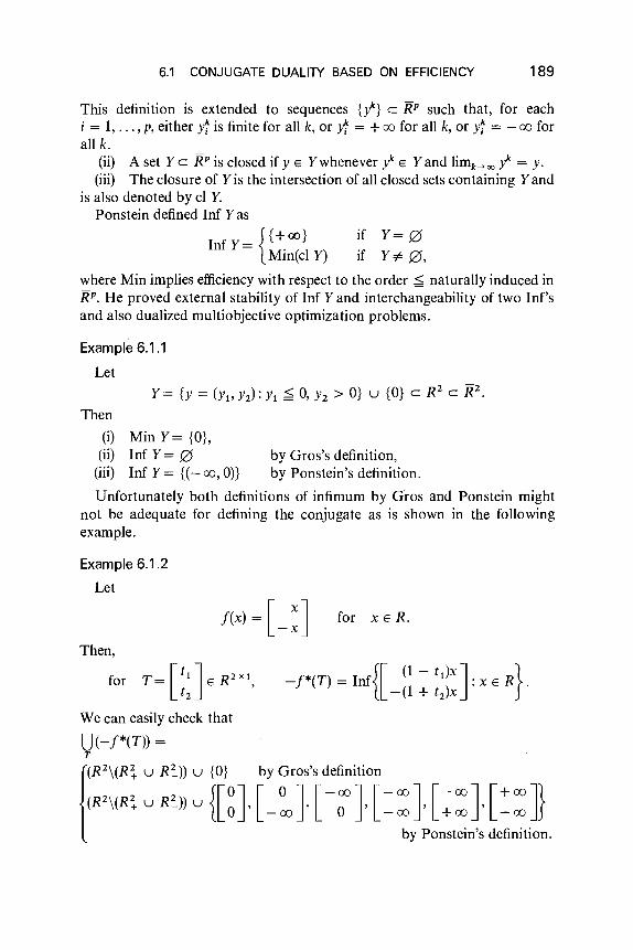
6.1 CONJUGATE DUALITY BASED ON EFFICIENCY 189
This definition is extended to sequences {yk} c RP such that, for eachi = 1, ... , p, either y~ is finite for all k, or y~ = +00 for all k, or y~ = - 00 forall k.
(ii) A set Yc RP is closed if y E Ywhenever yk E Yand limk~oo yk = y.
(iii) The closure of Yis the intersection of all closed sets containing Yandis also denoted by cl y.
Ponstein defined Inf Yas
Inf Y= {{+00 } if Y= 0Min(cl Y) if Y"# 0,
where Min implies efficiency with respect to the order ~ naturally induced inRP. He proved external stability of Inf Yand interchangeability of two Inf'sand also dualized multiobjective optimization problems.
Example 6.1.1
Let2 -2
Y= {y = (Yl' Yz): Yl ~ 0, Y2 > O} u {O} eRe R .
Then
(i) Min Y= {O},(ii) Inf Y= 0 by Gros's definition,
(iii) Inf Y= {(- 00, On by Ponstein's definition.
Unfortunately both definitions of infimum by Gros and Ponstein mightnot be adequate for defining the conjugate as is shown in the followingexample.
Example 6.1.2
Let
for x E R.
* - {[ (1 - t 1)xJ. }-f (T) - Inf -(1 + t2)x . x E R .
Then,
for T= [::J E R2 x l,
We can easily check that
U(-f*(T)) =T
{( R 2 \ ( R ~ u R~)) u {O} by Gros's definition
(R'\(R~ u R')) u {[~H -~H -n [=:}£t:)'J~:I
190
Hence,
6 CONJUGATE DUALITY
(Gros)
(Ponstein),
which does not contain
1(0) = [~J
6.2 Conjugate Duality Based on Weak Efficiency
As has been shown in the previous section, the duality result is not alwaysreflexive if we use the vector dual variable (Le., W(O) ~ W**(O), generally).Recently Kawasaki [K2, K3] gave some new notions and some fundamentaltools and results needed for developing the reflexive duality theory ofmultiobjective optimization problems. His approach is based on weakefficiency instead of usual efficiency. Weak efficiency is easier to deal withthan efficiency, since it is directly related to scalarization. (See Corollary3.4.1.) Moreover, his primal problems are also defined by vector-valuedpoint-to-set maps (called relations in his papers).
The above two facts are undesirable from the practical point of view inmultiobjective optimization. However, his results can enrich the conjugateduality theory and so are well worth paying attention to. Hence, in thissection, we overview Kawasaki's conjugate duality theory. In order to avoidmaking this section longer than needed, we omit all the proofs of theorems,propositions, and lemmas. If the reader is interested, please see the originalpapers. We should also note that some notations and terms in this section aredifferent from the original ones. Particularly, we often add the modifier weaknot to confuse the concepts in Sections 6.1 and 6.2.
6.2.1 Weak Supremum and Infimum
In this subsection, the definition and some fundamental properties of weaksupremum and infimum will be given. The p-dimensional point consisting ofa common element IY. E R is simply denoted by IX. Let
R~ = RP u Hoo}.
Of, course, -00 < y < +00 for all Y E RP. Let
K = intRP u {OJ.
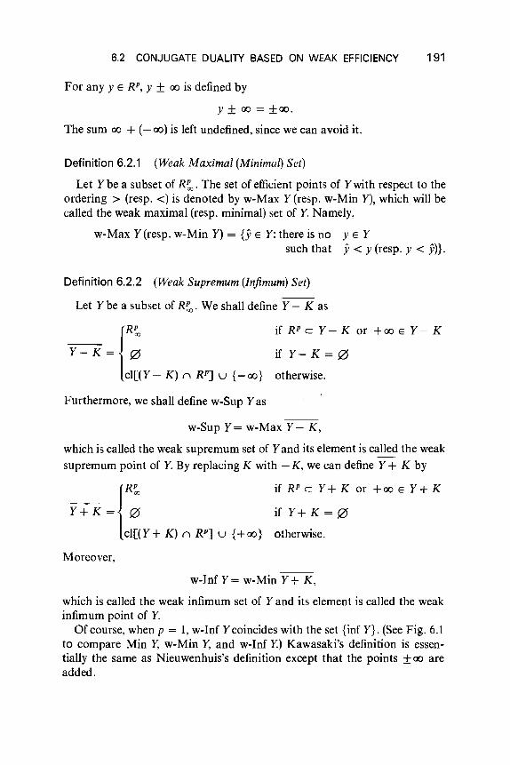
6.2 CONJUGATE DUALITY BASED ON WEAK EFFICIENCY 191
For any y E RP, Y ± 00 is defined by
y ± 00 = ±oo.The sum 00 + (- (0) is left undefined, since we can avoid it.
Definition 6.2.1 (Weak Maximal (Minimal) Set)
Let Ybe a subset of R~. The set of efficient points of Ywith respect to theordering> (resp. <) is denoted by w-Max Y (resp. w-Min Y), which will becalled the weak maximal (resp. minimal) set of Y. Namely,
w-Max Y(resp. w-Min Y) = {y E Y: there is no y E Ysuch that y < y (resp. y < y)}.
Definition 6.2.2 (Weak Supremum (Infimum) Set)
Let Ybe a subset of R~. We shall define Y- K as
{R ~ if RP c Y - K or +00 E Y - K
Y-K= 0 ifY-K=0
cl[( Y- K) n RP] u {- 00 } otherwise.
Furthermore, we shall define w-Sup Yas
w-Sup Y= w-Max Y- K,
which is called the weak supremum set of Yand its element is called the weak
supremum point of Y. By replacing K with - K, we can define Y+ K by
{R ~ if RP c Y + K or + 00 E Y + K
Y+K= 0 if Y+K=0
cl[( Y+ K) n RP] u {+ 00 } otherwise.
Moreover,
w-Inf Y= w-Min Y+ K,
which is called the weak infimum set of Yand its element is called the weakinfimum point of Y.
Of course, when p = 1, w-Inf Ycoincides with the set {inf Y}. (See Fig. 6.1to compare Min Y, w-Min Y, and w-Inf Y.) Kawasaki's definition is essen-tially the same as Nieuwenhuis's definition except that the points ±00 areadded.
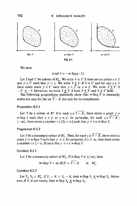
192
Min Y
We have
6 CONJUGATE DUALITY
w-Min Y
Fig. 6.1.
w-Inf Y
w-inf Y = - w-Supt- Y).
Let Yand Y' be subsets of Rfo. We write Y ~ Y' if there are no points y E Yand y' E y' such that y' < y. We write Y ~ Y' if Y ~ Y' and for any y E Y
-+there exists some y' E Y' such that y < y' or y = y'. We write Y ~ Y' if
+-- Y' ~ - Y. Moreover, we write Y <t. Y' if both Y ~ Y' and Y ~ Y' hold.
-+ H -+ +-The following propositions essentially show that w-Sup Y is externally
stable not only for the set Y - K but also for its complement.
Proposition 6.2.1
Let Y be a subset of RP. For each y E Y - K, there exists a point y' E
w-Sup Y such that y < y' or y = y'. In particular, for each y E Y - K\{-oo}, there exists a number t E [0, +00] such that y + t E w-Sup Y.
Proposition 6.2.2
Let Y be a nonempty subset of Rfo. Then, for each y 1= Y - K, there exists apoint y' E w-Sup Ysuch that y' < y. In particular, if y -::f. 00, then there existsa number t E [ - 00, 0) such that y + t E w-Sup Y.
Corollary 6.2.1
Let Y be a nonempty subset of Rfo. If w-Sup Y -::f. ±{00 }, then
(w-Sup Y + int R~.)" = Y - K in Rfo.
Corollary 6.2.2
Let Y1, Y2 C Rfo. If Y1 - K c Y2 - K, then w-Sup Y1 ~ w-Sup Y2 • More-->
over, if Y1 is not empty, then w-Sup Yt S w-Sup Y2 •
6.2 CONJUGATE DUALITY BASED ON WEAK EFFICIENCY 193
Lemma 6.2.1
Let Ybe a subset of R~. Then we have
w-Inf(w-Sup Y) = w-Sup y,
w-Sup(w-Inf Y) = w-Inf Y.
6.2.2 Weak Conjugate Maps and P-Regularization
This subsection is devoted to weak conjugate maps and P-regularizationof vector-valued point-to-set maps. The definition of a new type of conjugatemaps is based on the weak supremum instead of the usual efficiency.
Definition 6.2.3 (Weak Conjugate Map and Weak Biconjugate Map)t
Let F be a point-to-set map from R" into R~. The weak conjugate mapw-F*: R" -+ R~ of F is defined by
w-F*(x*) = w-Sup U[(x*, x) - F(x)].x
Furthermore, the weak biconjugate map w-F**: R" -+ R~ is defined by
w-F**(x) = w-Sup U[(x*, x) - w-F*(x*)].x·
Proposition 2.1.26 shows that the conjugate functionf* of a scalar-valuedfunction f is a closed convex function, which is the pointwise supremum ofthe collection of all affine functions h such that h ~f (Proposition 2.1.25).The set of closed convex functions f is often denoted by r. This class isextended to vector-valued point-to-set maps.
Definition 6.2.4 (Class P)
The set of point-to-set maps G: W -+ R~ that which can be written as
G(x) = w-Sup U(x~, x) + ay )
y
is denoted by P(R"), or simply by P, where x~ E R", ay E R~ for all vand theset of indices v is not empty.
For two point-to-set maps F and G from R" into R~, we write F ~ G ifF(x) ~ G(x) for all x E W.
t Cf. Definition 6.1.1.

194 6 CONJUGATE DUALITY
Definition 6.2.5 (P-Regularization)
Let F be a point-to-set map from R" into R~. The point-to-set map Fdefined by
F(x) = w-suP[ U «x*, x) + a)](x'" >+ a '" Fx E Rlf
• a E R~
is called the P-regularization of F.
The following theorem shows the relationship between the r p-
regularization and the weak conjugate map.
Theorem 6.2.1
Let F be a point-to-set map from R" into R~, and F be the P-regularization of F. Then
(i)(ii)
(iii)(iv)(v)
FeP,F~F
~'
if G e P and G ~ F, then G ~ F.- +-+F = F holds if and only if F E P,F = w-F**, if F(x) is not identically empty.
Next, we shall give a characterization of P.
Definition 6.2.6 (Scalarizable Point-To-Set Map)
Let F be a point-to-set map from W into R~. We call F scalarizable if Fsatisfies
w-Sup F(x) = F(x) ::p 0 forall xeRn•
Remark 6.2.1By Lemma 6.2.1, F is scalarizable if and only if
w-Inf F(x) = F(x) ::p 0 for all x e R".
Definition 6.2.7 (Scalarized Function)
Let F be a scalarizable point-to-set map from W into R~, and let a bean arbitrary point of RP. Let A be the diagonal set of RP, and letAoo = Au {±oo}. Namely
A = {(X e Rr :« e R} and Aoo = {(X:rx E R).
Then, by Propositions 6.2.1 and 6.2.2, the set (a + Aoo) n F(x) is a singleton,and its element can be expressed uniquely as a + Fa(x), where Fix) e R. Thus

6.2 CONJUGATE DUALITY BASED ON WEAK EFFICIENCY 195
we can define the function Fa:R" -+ R, which is called the scalarized functionof F through a.
We can characterize r p in terms of scalarizable point-to-set maps andscalarized functions.
Theorem 6.2.2
Let F be a point-to-set map from W into R~. Then F is contained in P ifand only if F is scalarizable and all the scalarized functions of Farecontained in r-.
Proposition 6.2.3
For any scalarizable point-to-set map F,
(Fa)* = (w-F*)_a
(Fa)** = (w-F**)a
for all a E RP,
for all a E RP,
6.2.3 Weak Subdifferentials of Point-To-Set Maps
In this subsection we shall define weak subgradients of vector-valuedpoint-to-set maps.
Definition 6.2.8 (Weak Subgradient and Weak Subdifferentia0t
Let F be a point-to-set map from W into R~. F is said to be weaklysubdifferentiable at (x; y) E R" x R~ if y E F(x) n RP and there exists somex* E R" such that
(x*, x' - x) + y ~ F(x') for all x' ERn.
We call x* a weak subgradient of F at (x; y). The set of all weak subgradientsof F at (x; y) is called the weak subdifferential of F at (x; y) and is denoted byw-oF(x; y). Let
w-oF(x) = U w-oF(x; y).yo;F(x)
Lemma 6.2.2
Let F be a point-to-set map from W into R~. Then
(i) w-oF(x; y) c w-o(w-F**)(x; y) for all x E R" and y E RP,(ii) If w-F**(x) c F(x), then w-oF(x; y) = w-o(w-F**)(x; y) for all
y E w-F**(x),
t a. Definition 6.1.2.

196 6 CONJUGATE DUALITY
(iii) y is contained in F(x) n w-Min[Ux' F(x')] n RP if and only ifoE w~oF(x; y),
(iv) x* E w-oF(x; y) if and only if <x*, x) E Y + F*(x*) and y E
F(x) n RP,(v) if x* E w-oF(x; y), then x E w-o(w-F*)(x*; (x*, x) - y). In partic-
ular, if F E r p, then the above two conditions are equivalent to each other.
Corollary 6.2.3
Let F be a point-to-set map from R" into R~. Then
(i) w-oF(x) c: w-o(w-F**)(x) for all x E R",(ii) if w-F**(x) c: F(x), then w-oF(x) = w-8F**(x),
(iii) F(x) n w-Min[Ux' F(x')] n RP =1= 0 if and only if 0 E w-8F(x),(iv) x* E w-oF(x) if and only if (x*, x) E F(x) + w-F*(x*),(v) if x* E w-oF(x), then x E w-8(w-F*)(x*). In particular, if F E P, then
the above two conditions are equivalent to each other.
We can obtain the relationship between weak subdifferentials of sealariz-able point-to-set maps and subdifferentials of scalarized functions.
Proposition 6.2.4
Let F be a sealarizable point-to-set map from R" into R~. For any x E R"and y E F(x) n RP, we have
w-8F(x; y) = 8Fy(x).
6.2.4 Duality
In this subsection, by using the results obtained in the previous sub-sections, we provide duality results similar to those in Section 6.1. First, let <I>be a point-to-set map from R" x R m into R~. We assume that it is notidentically empty on R" x {O}.
The primal problem can be written as
(P) find xE R" such that
<I>(x,O) n W-Min[V<I>(x, O)J n RP =1= 0·
This problem can be equivalently rewritten as
(P) find xE R" such that
<I>(x,O) n W-Inf[V<I>(X,O)J n RP =1= 0·
6.2 CONJUGATE DUALITY BASED ON WEAK EFFICIENCY 197
This problem can be imbedded into a family of perturbed problems
(Pu) find x E R" such that
<I>(x, u) n w-Inr[V<I>(x, U)] r. RP =F 0.
The dual problem and the family of perturbed dual problems are given as
(D) find ~ E R" such that
- w-<I>*(O,~) n w-su{V-w-<I>*(O, 2)] n RP =F 0,
(D,,) find ~ E R" such that
-w-<I>*(Jl,~) n w-su{Y-w-<I>*(jl, Pc)] n RP '# 0.
Define point-to-set maps W: Rm --+ RP (which is slightly different from WinSection 6.1 though the same symbol is used) and V: R" --+ RP by
W(u) = W-Inf[V<I>(x, U)] and V{Jl) = -w-su{V-w-<I>*(jl, Pc)].
We denote W(O) and - V(O) by w-Inf P and w-Sup D, respectively. Thefollowing lemma is analogous to Lemma 6.1.3.
Lemma 6.2.3
(i) w-W*(Pc) = w-<I>*(O, Pc) for all Pc E B",(ii) w-V*(x) = w-<I>**(x, O) for all x E R". In particular, if <I> E
P(R" x Rm), then w-V*(x) = <l>(x, 0) for all x E R".
Lemma 6.2.4 t
(i) w-Sup(D) = w-W**(O),(ii) if <I> E P(R" x Rm), then w-Inf(P) = -w-V**(O).
The weak duality theorem can be strengthened to the following.
Proposition 6.2.5~
w-Sup(D) ~ w-Inf(P).+-+
Convexity of <I> and Ware related via their scalarized functions.
t Cf. Lemma 6.1.4.t Cf. Corollary 6.1.4.
198
Lemma 6.2.5 t
6 CONJUGATE DUALITY
If cI> is scalarizable and every scalarized function of cI> is convex, then everyscalarized function of W is also convex.
Stability of the primal (resp. dual) problem can be defined in terms ofscalarized functions of W (resp. V). We also introduce a new conceptnormality extended from the case of scalar optimization.
Definition 6.2.9 (Normality)f.
If every scalarized function of W (resp. V) is lower semicontinuous andfinite at 0, then the primal (resp. dual) problem (P) (resp. (D)) is said to benormal.
Definition 6.2.10 (Weak Stability)§
If every scalarized function of W (resp. V) is weakly subdifferentiable at 0,then the primal (resp. dual) problem (P) (resp. (D)) is said to be weakly stable.
Proposition 6.2.6
Suppose that cI> E P, that w-Inf(P) is a nonempty subset of RP, and that foreach a E RP there exists Xa E R" such that cI>a(xa, \) is finite and continuous at0. Then (P) is weakly stable.
Proposition 6.2.7"
IfcI> E P, then the following three conditions are equivalent to each other:
(i) (P) is normal,(ii) (D) is normal,
(iii) w-Inf(P) = w-Sup(D) and this set is a nonempty subset of RP.
Proposition 6.2.8
(i) For any 2 E R" and y E R~, Y E -w-cI>*(O, 2) r, w-Sup(D) (', RP ifand only if,{ E w-o(w-W**XO; y).
(ii) Suppose that cI> E P. For any x E R" and y E R~, Y E cI>(X, 0) (',w-Inf(P) (', RP if and only if x E w-o(w- V**XO; - y).
t cr. Lemma 6.1.2.I Cf. Ekeland and Temam [EI. Definition m.2.l].§ cr. Definition 6.1.3.110. Ekeland and Temam [E1, Proposition III.2.l].

6.2 CONJUGATE DUALITY BASED ON WEAK EFFICIENCY 199
Proposition 6.2.9
If <I> E P, the following three conditions are equivalent to each other:
(i) (P) is weakly stable,(ii) W(O) is a nonempty subset of RP, and Wis weakly subdifferentiable at
(0; y) for any y E W(O).(iii) w-Inf(P) = w-Sup(D) = w-Max(D), and this is a nonempty subset of
RP, where w-Max(D) = w-Maxjj], -w-<I>*(O, A) - K].
The main strong duality theorem is given as follows.
Theorem 6.2.3 t
Suppose that <I> E P and that the primal problem (P) is weakly stable.Then the dual problem (D) has at least one solution. If x E Rn is a solution of(P), then there exists a solution ~ of (D) such that
<I>(x,O) n - w-<I>*(O, ~) :t- 0or equivalently
(0, ~) E w-8<1>(x, 0).
Conversely, if x E R" and ~ E R" satisfy the above relationship, then x is asolution of (P), 1 is a solution of (D) and
<I>(x,O) r. -w-<I>*(O,~) c w-Inf(P) n w-Sup(D) n RP.
Remark 6.2.2
The above duality theorem satisfies a reflexivity. In fact, we can exchangethe roles of (P) and (D) in Theorem 6.2.3.
As a matter of fact, as is shown in the following proposition, the primalproblem (P) can be reduced to ordinary scalar optimization problem when <I>is scalarizable.
Proposition 6.2.1 0
If <I> is scalarizable, then x E R" is a solution of (P) if and only if there existsa E RP such that x is a solution of the following scalar optimization problem(Pa):
(Pa) minimize <l>ix, 0).
t cr. Theorem 6.1.1.
200 6 CONJUGATE DUALITY
6.2.5 Weak Lagrangians and Weak Saddle Points
for x ERn, A E Rm
In this subsection, we shall introduce a weak Lagrangian of the primalproblem (P) relative to the given perturbations C1> and clarify the relationshipbetween the pairs of solutions of (P) and (0) and weak saddle points of theweak Lagrangian.
Definition 6.2.11 (Weak Lagrangian)t
The point-to-set map w-L: W x R'" -.. R~, defined by
w-L(x, A) = w-Inr[v(C1>(x, u) - (A, u»)]
is called the weak Lagrangian of the primal problem (P) relative to the givenperturbations.
Definition 6.2.12 (Weak Saddle Point)t
A point (x,~) E R" x R'" is called a weak saddle point of the weakLagrangian w-L, if there exists y E w-L(x.~) n RP such that
w-L(x, A) ~ Y ~ w-L(x, ~) for all x E R" and A. E B".
Let
w-Inf w-Sup w-L = w-Inf V[w-Sup Vw-L(x, A)],
w-Sup w-Inf w-L = w-Sup V[w-Inf Vw-L(x, A)].
Proposition 6.2.11
w-Sup w-Inf w-L ~ w-Inf w-Sup w-L.-Proposition 6.2.12
The following two conditions are equivalent to each other:
(i) (x,~) is a weak saddle point of w-L and y E L(x,~) satisfiesw-L(x, A) ~ Y ~ w-L(x,~) for all x E R" and A E R'",
(ii) y E w-Int'[l], w-L(x,~)] n w-SUP[Ul w-L(x, A)] n RP.
t Cf. Definition 6.1.4.: Cf. Definition 6.1.5.

6.3 CONJUGATE DUALITY ON STRONG SUPREMUM AND INFIMUM 201
Proposition 6.2.13
(x,~) E W x R" is a weak saddle point of w-L if and only if there existsa E RP such that (x,~) is a saddle point of the scalarized function (w-L)a'
The primal problem and the dual problem can be represented by the weakLagrangian as follows.
Proposition 6.2.14t
(i) -w-<I>*(O, A.) = w-Inf Ux w-L(x, A.) for all A. E R" and hencew-SuP(D) = w-Sup w-Inf w-L,
(ii) if <I> E P, then <I>(x,O) = w-Sup U.. w-L(x, A.) for all x E R" and hencew-Inf(P) = w-Inf w-Sup w-L.
Theorem 6.2.4:
If <I> E P, then the following conditions are equivalent to each other:
(i) (x, 1) E R" x B" is a weak saddle point of the weak Lagrangian,(ii) x and 1 are solutions of (P) and (D), respectively, and <Il(x,O) /I
-w-<I>*(O,~) =F 0,(iii) <l>(x,O) /I - w-<I>*(O, 1) 11 RP =F 0.
Theorem 6.2.5~
Suppose that <I> E P and that (P) is weakly stable. Then the followingconditions are equivalent to each other:
(i) xis a solution of (P),(ii) there exists ~ E B" such that (x,~) is a weak saddle point of the weak
Lagrangian. In this case ~ is a solution of (D).
6.3 Conjugate Duality Based on Strong Supremum and Infimum
Brumelle [B21] took an approach different from Tanino and Sawaragi's orKawasaki's to derive duality for convex multiobjective optimization prob-lems. His definitions of conjugates and subgradients are all based on theconcept of strong supremum and infimum, which are the least upper boundand the greatest lower bound, respectively, for a partially ordered set. Since
t cr. Proposition 6.1.14 and 6.1.15.I cr. Theorem 6.1.2.§ cr. Theorem 6.1.3.
202 6 CONJUGATE DUALITY
strong infimum essentially implies componentwise infimum, we can directlyextend the well-known results concerning conjugate functions and sub-gradients of scalar-valued convex functions. (See Section 2.1.)
Brumelle also concentrated on properly efficient solutions, which can becompletely characterized as solutions of scalarized problems with negative(or positive) weighting vectors. (See Theorems 3.4.1 and 3.4.2.) Since everyefficient solution of a linear multiobjective optimization problem is properlyefficient (Corollary 3.1.1), his results are particularly meaningful in the linearcase.
In this section we overview the conjugate duality according to Brumelle[B21]. As in Section 6.2, the proofs of theorems, propositions, and lemmasare omitted.
6.3.1 Strong Supremum and Infimum, Conjugate Functions,and Subgradients
We provide some fundamental concepts-strong supremum, conjugatesand subgradients-in this subsection. They were also used by Zowe [Z9,ZlO]. However Zowe and Craven [C17] considered problems of findingstrongly supremal points (i.e., strongly optimal solutions), which are differentfrom the multiobjective optimization problems in this book. It might bebetter to call the concepts defined in this section without the modifier strong,since they are direct extensions from the concepts in the scalar case.However, in this book, we attach it in order to distinguish them from theconcepts defined earlier.
First we define strong supremum and maximum of a set in the spaceR~ = RP u {±oo}.
Definition 6.3.1 (Strong Supremum (Infimum) and Maximum (Minimum))
Let Ybe a subset of R~. A point yis said to be a strong supremum of Yanddenoted by y = sup Y if and only if y is an upper bound for Y in R~ (i.e.,y ~ Y for any Y E Y)and y ~ ji whenever ji is any other upper bound of Y. IfYis empty, then sup Y= - 00. If, in addition, y E Ythen we call y a strongmaximum of Yand denote it by max Y. Strong infimum (inf Y) and strongminimum (min Y)can be defined analogously.
Note that sup Y is a unique element of R~ for any Yc R~ and that ifsup YE RP, then (sup Y)i = SUP{Yi: Y E Y}. Namely, sup Yis essentially thecomponentwise supremum of Y.
6.3 CONJUGATE DUALITY ON STRONG SUPREMUM AND INFIMUM 203
Definition 6.3.2 (Strong Conjugate and Strong Biconjugate)t
Letf be a convex function from R" to Rt,. The strong conjugate functionf* off is the function from W x n to Rt, defined by
f*(T) = sup{Tx - f(x) : x E W}.
Furthermore, the strong biconjugate function f** : W --+ Rt, is defined by
f**(x) = sup{Tx - f*(T) : T E W x "}.
Note that if f*(T) E W, then f*(T) = (fi(t!), ... ,f;WW, where T=(t1, ... , tP)T with each ti ERn.
Definition 6.3.3 (Strong Closures'
Let f be a vector-valued convex function from R" to Rt,. The strongclosure of J, which is denoted by el J, is defined by (el f)(x) = inf {y : (x, y) E
cl(epif)} iff never takes the value -00 and (elfXx) = -00 iff(x) = -00 forsome x. The function f is said to be strongly closed iff = cl f.
Proposition 6.3.1§
Iff is a convex function from R" to RP, then f* is convex and f** = elf.
Example 6.3.1
As a simple example, consider
f(x) = (x, - X)T
Then
f*(T)={O+00
for x E R.
if T= (1, -1)
otherwise.
Thus, f*(T) takes the infinite value too often.
Next, we define strong subgradients of convex vector-valued functions.
Definition 6.3.4 (Strong Subgradient) II
Let f be a convex vector-valued function from R" to Rt,. A matrixT E RP x n is said to be a strong subgradient off at xif
f(x) ~f(x) + T(x - x) for any x ERn.
t Cf. Definition 2.1.20, 6.1.1, and 6.2.3.I Cf. Definition 2.1.19.§ Cf. Proposition 2.1.26."Cf. Definition 2.1.23, 6.1.2, and 6.2.8.

204 6 CONJUGATE DUALITY
The set of strong subgradients off at xis called the strong subdifferential offat x and is denoted by of(x). If of(x) is not empty, f is said to be stronglysubdifferentiable at x. of*(T) can be defined analogously.
Proposition 6.3.2
Letf be a convex function from R" to R~. Thenp
of(x) = X oJ;(x) = {T= (t1, ••• , tpl: ti E oJ;(x), i = 1, ... ,p}.
i=l
Proposition 6.3.3 t
Letf be a proper convex function from R" to R~. Then
f(x) + f*(T) ~ Tx
for all x E R" and T E RPx n, with equality holding if and only if T E of(x). Iffis closed, then equality is obtained if and only if x E of*(T).
6.3.2 Proper Efficiency and Zerolike Matrix
In this subsection we consider the characterization of properly efficientsolutions of a convex vector-valued function in terms of zerolike matrices.Letfbe a proper convex function from R" to R~. We should recall that xis aproperly efficient solution of a multiobjective optimization problem
minimize f(x)
if and only if x minimizes the scalar-valued function </1,f(x» for some/1 E int R~ (Theorems 3.4.1 and 3.4.2). In this case we simply say that xisproperly efficient for f.
Definition 6.3.5 (Zerolike Matrix)
A matrix T E RPx n is said to be zerolike (written T", 0 or 0 '" T) if thereexists a vector /1 E int R~ such that the n vector TT/1 = O.
Proposition 6.3.4
Let f be a proper convex function from R" to R~. Then xis properlyefficient for f if and only if there exists a zerolike T E of(x), in other words, ifand only if there exists a zerolike T E RP x n such that
f(x) E min{f(x) - Tx: x E R"}.
We must note that, when T E of(x), Iii can be interpreted as the rate ofchange of the ith objective per unit change in the jth activity at x.
t Cf. Proposition 2.1.27 and 6.1.3.

6.3 CONJUGATE DUALITY ON STRONG SUPREMUM AND INFIMUM 205
6.3.3 Duality
Now we can derive duality in convex multiobjective optimization based onthe preceding concepts. Though the original paper by Brumelle [B21]generalized the duality theory of convex bifunctions by Rockafellar [R8], werewrite it in a form analogous to Sections 6.1 and 6.2.
Let qJ be a function from W x R m to R~. The function qJ is assumed to beproper and convex throughout this section. The primal problem is
(P) minimize qJ(X, 0).
We would like to find xthat is properly efficient for qJ(',0) (simply for qJ). Inview of Proposition 6.3.4, for each TE R"":", we define the convex functionqJT: R" x R'" -> R~ as
qJT(X, u) = <p(x, u) - Tx.
The notation (u, T) ......, 0 means u = 0 and T......, O. Dually, for each u, let
<p:(T, A) = <p*(T, A) - Au.
We consider two kinds of perturbed problems that are regarded as strongoptimization problems
(PT) minimize qJT(X, 0),
(DT) maximize -<pt(T,A) = -<p*(T,A) (Tis fixed).
Definition 6.3.6 (Admissibility)
If xis a minimizing solution of (PT), that is, if
<PT(X,O) = min{qJT(x, 0): x ERn},
for some zerolike T, then x is said to be admissible for qJ. Dually, if A is amaximizing solution of (DT) , that is, if
-<p*(T,A) = max{-<p*(T, A): A E RPxm},
for some zerolike T, then Ais said to be admissible for <p*.
Proposition 6.3.5
The following three conditions are equivalent:
(i) xis properly efficient for tp,
(ii) xis admissible for qJ,(iii) there are some u E int R~ and some t E fT(/l) such that
for all (x, T) E R" x fT(/l),
where
206 6 CONJUGATE DUALITY
In view of this proposition we might say that 1\ is properly efficient for cp* ifthere are J1. E int R~ and T E ff(J1.) such that
<J1., -cp*(7; 1\) ~ <J1., -<p*(T, A) for all (T, A) E ff(J1.) x R'":",
such thatTE f/(J1.)for all
Note that if 1\ is properly efficient for <p*, then 1\ is properly efficient for- <p*(T, .) for some T", 0, and hence 1\ is admissible for cp*; however, theconverse statements do not hold.
In view of Proposition 6.3.5, the set of properly efficient solutions of (P) isequal to the set of admissible points, which is the union of the solution sets of(PT) with T", 0. Hence, we may define the dual problem (D) of (P) as theproblem of finding the set of properly efficient points of <p*. Namely
(D) find 1\ E RP x m such thatthere exist J1. E int RP and<J1., -<p*(7; 1\) ~ <J1., -<p*(T, A)(T, A) E ff(J1.) x RPxm.
Note that (D) is different from the problem
maximize -<p*(0, A) subject to A E R'":",
However, in this case, the set of properly efficient points is included in the set
U{1\ E RPxm: -<p*(T, 1\) = max{-<p*(T, A); A E RPxmnT-O
but is not equal to it. A drawback of Brumelle's formulation is that theunperturbed dual problem involves the dual perturbation T. This causesexcessive sensitivity of the problem (See Ponstein [P3].)
Brumelle defined another efficiency concept for <p*, motivated byIsermann's results for linear problems.
Definition 6.3.7 (Isermann Efficiency)
If there exists some zerolike T such that
-<p*(7; 1\) s -<p*(T, A) forno T",OERPx n and no
then 1\is said to be Isermann efficientfor <p* .
We define the perturbation functions wT on R m and Vu on R'":" as
wT(u) = inf{tpT(x, u): x ERn}
and
6.3 CONJUGATE DUALITY ON STRONG SUPREMUM AND INFIMUM 207
respectively. The functions W T and Vu are convex with dom W T ={u : CPT(-, u) =1= +oo} and dom Vu = {T: <p*(T, .) =1= +oo}. The following is aweak duality theorem.
Theorem 6.3.1
CPT(X, u) ~ - <p;(T, A).
Consequently, for each u E B" and TE R'":",
wT(u) ~ - vu(T),
and CPT(X,O):::;; -<p*(T, A) does not hold for any x ERn, A E R'":" andT",OERpx n.
Corollary 6.3.1
If CPT(X, 0) = -<p*(7; A), TT fJ. = 0, and fJ. E int R~, then xand Ahave thefollowing properties:
(i) x minimizes (fJ., CPt<x, 0» for x ERn, and (7; A) maximized(fJ., -<p*(T, A» for (T, A) E .r(fJ.) x R'":", This xand Aare properly efficientfor tp and <p*, respectively.
(ii) x is efficient for cP; i.e.,
cp(x, 0) ~ cp(x, 0) for no x ERn,
(iii) if Tx = 0, then A is Isermann efficient for <p*.
The result corresponding to Lemma 6.1.3 and Lemma 6.2.3 is thefollowing.
Lemma 6.3.1
(i) For each T E W x n, w¥(A) = <p*(T, A) for all A,(ii) if cP is closed, then for each u E R'", v;(x) = cp(x, u) for all x.
Definition 6.3.8 (Strong Normality)t
If wT is closed at u, problem (P) is said to be strongly normal at (u, T).Similarly, if Vu is closed at T, problem (D) is said to be strongly normal at(u, T). If (P) (resp. (D)) is strongly normal at (u, T) for each (u, T) '" 0, then (P)(resp. (D)) is said to be strongly normal.
t cr. Definition 6.2.9.

208 6 CONJUGATE DUALITY
Theorem 6.3.2 t
If <p is closed, then the following are equivalent:
(i) (P) is strongly normal at (u, T),(ii) (D) is strongly normal at (u, T),
(iii) wT(u) = - vu(T).
Lemma 6.3.2
If qJ is closed, then anyone of the following conditions is sufficient forguaranteeing that (P) (or equivalently (D)) is strongly normal at (0, T):
(i) OEri ({u:<p(',u) '1= +oo}).(ii) TE ri ({T': <p*(T',.) '1= +oo}).
(iii) <p is polyhedral (i.e., epi <p is a polyhedral convex set) and<p(', 0) '1= +00.
(iv) <p* is polyhedral and <p*(T, .) '1= + 00.
We can now define the strong Lagrangian for <PT and its saddle point.
Definition 6.3.9 (Strong Lagrangian and Strong Saddle Point)t
The strong Lagrangian L: R" x Rr":" -+ R~ of the primal problem (P) isdefined by
L(x, A) = inf{<p(x, u) - Au: u E Rm} .
Moreover, the strong Lagrangian LT of the problem (PT) is defined by
LT(x, A) = inf{<p~x, u) - Au: u E Rm} .
Clearly LT(x, A) = L(x, A) - Tx. A point (x, A) is said to be a strong saddlepoint of LT if
LT(x, A) s LT(x, A) s LT(x, A) for all x ERn, A E RPxm.
Theorem 6.3.3 ~
Suppose that ip is closed and let x ERn, A E RPx mand 0 ~ T E RPx ", Thefollowing conditions are equivalent:
(i) Problem (P) is normal at (0, T) and x and A are properly efficientsolutions of (P) and (D), respectively, with
<PT(X,O) = min{ <P~x, 0) : x ERn}
t cr. Proposition 6.2.7.~ Cf. Definition 6.1.4, 6.1.5, 6.2.11, and 6.2.12.§ cr. Theorem 6.1.2 and 6.2.4.
6.3 CONJUGATE DUALITY ON STRONG SUPREMUM AND INFIMUM 209
and
-<p*(T,A) = max{-<p*(T, A): A E RPx m} .
(ii) (x,A) is a strong saddle point of the strong Lagrangian LT'(iii) qJT(X, 0) ~ - <p*(T, A) (in which case equality must actually hold).
Theorem 6.3.4
Suppose that qJ is closed, that dom qJ(" 0) #- 0, and that T E RPx n is zerolike. If qJ is polyhedral or 0 E ri {u: qJ(x, u) =1= +co}, then the followingconditions are equivalent:
(i) x is a properly efficient solution of (P) and strongly minimizesqJTL 0),
(ii) (x, A) is a strong saddle point of the strong Lagrangian LTfor someAE sr»,
(iii) (T, 0) E oL(x, A) for some AE Rpx m.
Theorem 6.3.5
Suppose that <p is polyhedral and that 0 rt aff(dom <p(', 0)), where aff(S)denotes the affinehull of a set S. Ifxis an efficientsolution of the problem (P),then there exists (,T, A) such that -<p*(f, A) = <p(x,O) and A is Isermannefficient.
7 METHODOLOGY
This chapter deals with methodology for practical implementation ofmultiobjective decision making. Above all, utility (value) analysis andinteractive programming methods play key roles in this area. Our aim in thischapter is not merely to introduce these methods, but to discuss criticalpoints. For details and practical implementation of utility (value) analysis,Keeney and Raiffa [K6] is excellent. Regarding interactive programmingmethods, Chankong and Haimes [C6] and Hwang and Masud [HI7]include good surveys. Here, we shall emphasize controversial points of thetypical methods from a viewpoint of practical implementation and give adirection toward future research.
7.1 Utility and Value Theory
Following the same notations as in the preceding chapters (which may be alittle different from those of other literatures), let X denote the set ofalternatives, and let each of its elements be evaluated by several criteria orobjective functions j.: X --+ R 1 (i = 1, ... , p). In the utility and value theory,such criteria for evaluating alternatives are often called attributes. In thissection, we do not distinguish these terminologies so long as there is no fear
210

7.1 UTILITY AND VALUE THEORY 211
of confusion. Preference of decision makers are supposed to be expressed onthe criteria space Y(in which each Yi reflects the criterion j.), rather than onthe set of alternatives itself. This section will be concerned with existence,representation, and uniqueness of a function u: Y~ R 1 representing thedecision maker's preference. Such a function representing the decisionmaker's preference is in general called a preference-preserving function or apreference function. In particular, following Keeney and Raiffa [K6], apreference function in decision making under uncertainty is called a utilityfunction, which is used to represent a general preference function in someother literatures. On the other hand, a preference function in decision makingunder certainty is called a valuefunction.
7.1.1 Preference Functions
This subsection will be concerned primarily with the existence problem ofpreference functions.
Definition 7.1.1 (Homomorphism)
Let (A, >-1) and (B, >-2) be some ordered sets. An onto mapping u: A ~ Bis called a homomorphism from (A, >-1) to (B, >-2) if the following holds forany at, a2 E A:
Then (A, >-d and (B, >-2) are called homomorphic by the mapping u.
Definition 7.1.2 (Isomorphism)
Let (A, >-1) and (B, >-2) be some ordered sets. An onto and one-to-onemapping u: A ~ B is called an isomorphism from (A, >-1) to (B, >-2), if thefollowing holds for any a 1
, a2 E A:
Then (A, >-1) and (B, >-2) are called isomorphic by the mapping u.
Remark7.1.1
A mapping u is an isomorphism if and only if both u and u- 1 arehomomorphisms.
212 7 METHODOLOGY
In order to make the treatment of the decision maker's preference easier,let us consider the set of real numbers with the usual inequality relation(Rl, » isomorphic or homomorphic to (Y, >-). A preference function isdefined as an isomorphic (or homomorphic) function u: (Y, >-) - (R1, ».
In examining the existence of such a preference function, it is meaningful toknow the structure of the set of real numbers. Among several characteristicsof the set of real numbers, the structure of order and addition is essential andalso plays an important role to our aim. Let Re denote the set of realnumbers with the natural order>. By this notation we discriminate such aset of primitive real numbers from R 1 with some topological properties. Thefirst noticeable point is that the natural order is a total order (Definition2.3.1). Further, let Ra denote the set of rational numbers. It is well knownthat the rational numbers are countable and dense in Ra itself, i.e., for anyCI., j3 E Ra
for some y ERa.
This encourages us to score each element of a totally ordered and countableset Y= {yl,y2, ... ,yk, ... } by the function u: Y-Ra such that for anypositive integer n,
(i) u(i) = 0,(ii) y"+l >- yk, 1 ~ Vk ~ n =? U(y"+l) = n,
y"+l < I, 1 ~ Vk::::;; n =? U(y"+l) = -no
Otherwise,
since there are integers i and j (1 ::::;; i, j ::::;; n) such that
or 1::::;; Vk ::::;; n.
This observation yields Theorem 7.1 below.For an uncountable set Y, we make use of the denseness of Ra in Re; that
is, for any CI., j3 E Re
CI.>j3=rt>y>j3 for some y ERa.
Of course, it is required that Y have a subset that is countable and order-dense in Y. (See Theorem 7.2 below.) It should be noted here that thedenseness of Ra does not imply its connectedness or continuity. In fact, there
7.1 UTILITY AND VALUE THEORY 213
are infinitely many gaps! in Ra. Similarly, there might be a gap in anuncountable set Ywith a subset countable and order-dense in Y. In defining apreference function Y -+ R 1
, special attention must be paid to such gaps. (Fora proof of Theorem 7.2 below, see, for example, Krantz et al. [K9] andFishburn [F7].)
Now recall that the set of real numbers is completed by making up thesegaps. To this end, irrational numbers are introduced, which produces thecontinuity property of Re.
In addition to the order structure, an operation on Re is defined calledaddition, +, by assigning a + b for any a, b E Re (which is again in Re) withthe following properties:
(1) (a + b) + c = a + (b + c),(2) a + b = b + a,(3) given a, b ERe, there exists c s Re such that a + c = b,(4) a < b => a + c < b + c, for any c e Re,
where property (4) connects the order and the addition on Re and is calledthe monotonicity of addition. An additive structure stands for a set togetherwith the operation of addition defined on the set. The additive structure onthe ordered set (Re, <) with the properties (l)-(4) provides a basis formeasurability (cardinality) of real numbers. The addition on Re along withthe order> leads to the well-known Archimedean property:
For given a > 0 and b > 0, there exists an integer n such that na > b.
In order to get a measurable preference function for (Y, >-), some notionscorresponding to the addition and the Archimedean property will benecessary (cf. Theorem 7.1.4 and Remark 7.1.4 below).
In the following, we shall list several existence theorems for preferencefunctions without proof. (For more details see, for exampl, Krantz et al.[K9], Fishburn [F7], and Keeney and Raiffa [K6].)
t For a totally ordered set (A, »0), the term a cut oj A implies to partition A in such a way thatA = A' u An,where A' and AU are disjoint subsets of A and for any a' E A' and an E An,we havea" >- d. For such a cut, the following three cases are possible: (i) The lower part A' has agreatest element and the upper part AU has a least element; (ii) the lower part A' has no greatestelement and the upper part AU has no least element; (iii) either A' has a greatest element and AUhas no least element or A' has no greatest element and AU has a least element.
For any cut of discrete sets, case (i) is necessarily possible. On the other hand, for any cut ofdense sets either case (ii) or (iii)is possible, whereas case (i) is never possible. In case (ii), we saythat the cut has a gap. For the set of rational numbers Ra, infinitely many cuts with gaps arepossible. For example, consider Ra = {IX E RalIX2 ~ 2} u {IX E RalQf2 > 2}. Irrationalnumbers are introduced to make up for such gaps in Ra so that only case (iii)arises for any cut inthe set of real numbers, which is defined as the set consisting of both Ra and the set of irrationalnumbers (Dedekind cut).

214
7.1.1.1 Value Functions
7 METHODOLOGY
Theorem 7.1.1
If (Y, >-) is a totally ordered set and if Y is countable, then there exists avalue function u: Y--> R 1 such that for every i, y2 E Y
i >- y2 ¢> uV) > U(y2).
Such a value function is unique up to a monotonically increasing function.'
Definition 7.1.3 (Order Dense)
Let >- be an order relation. Then a subset Z of Y is said to be >--orderdense in Y, if for any yl, y2 E y\Z there exists Z E Z such that
i>-y2=yl>-Z, Z>-y2.
Theorem 7.1.2
If (Y, >-) is a totally ordered set and if Y has a subset Z countable and>--order dense in Y, then there exists a value function u: Y--> R 1 such thatfor every i, y2 E Y
i >-l ¢> u(i) > U(y2).
Such a value function is unique up to monotonically increasing functions.
Remark 7.1.2
In cases of (Y, >-) being an weakly ordered set, we define the order o-' on theset of equivalent classes Y/", as
a »' b, a, b E Y/", ¢> x >- y, X E a, y E b.
t In the following, it is important to keep in mind what meaning the numerical values in(Re, » isomorphic or homomorphic to (Y, :>-) have. If these numbers make sense only for theirorders, they are said to be ordinal. Clearly, since their order relations are unchangeable by anymonotonically increasing transformation, the ordinal scale is rather redefined as the one that isunique up to a monotonically increasing transformation. Numerical values that make sense fortheir differences are said to be measurable or cardinal. There are two kinds of measurable scales:The first is the interval scale unique up to a positive affine transformation, which implies thatboth the order among the numerical values and the ratio (u(y!) - U(y2))j(V(Y') - V(y2)) areinvariant under a positive affine transformation v of u; that is, v = IX + flu, for fl > 0. Thisrelationship also says that the interval scale has arbitrariness of unit and origin, which can beseen in an example of the measure of temperature (Celsius and Fahrenheit). The second scale isthe ratio scale unique up to a positive similar transformation, which implies that both the orderamong the numerical values and the ratio u(y)jv(y) are invariant under a positive similartransformation v of u: that is, v = flu, for fl > 0. The ratio scale leaves arbitrariness of unit as inexamples of length and weight. In general, two preference functions u and v with the relationshipu = IX + flv for fl > 0, are said to be equivalent as cardinal measure.

7.1 UTILITY AND VALUE THEORY 215
Then, since j-' is clearly a total order, Theorem 7.1.1 and 7.1.2 can easily bemodified for a weakly ordered set (Y, >-). In Theorem 7.1.1, the result holdsfor a weakly ordered set (Y, >-) by replacing Y is countable with the set ofequivalent classes Y/- is countable. Theorem 7.1.2 holds for a weakly orderedset (Y, >-) by replacing (Y, >-) has a subset countable and >--order dense in Ywith the set ofequivalent classes Y/- has a subset countable and ';>!-order densein y/..J.
In order to reduce the selection of the maximal element of (Y, >-) to themaximization of the preference-representing function u('), the continuityproperty of u(.) encourages the existence of a maximal element under someappropriate conditions and applications of various optimization techniques.A mild, sufficient condition for continuity of value functions was derived byDebreu [D3].
Theorem 7.1.3
Suppose that the preference >- is defined on a subset Y of p-dimensionalEuclidean space RP with the natural topology 1:. Let 1:' be the inducedtopology of 1: to Y. Then, if Y is connected with respect to the topology 1:' andif for any y' E Y
p' := {y E Y: y >- y'} E T', and ¥" := {y E y: y -< y'} E T',
then there exists a continuous value function u such that for any yl, y2 E Y
yl >- y2 <0> U(yl) > u(y2).
Such a value function is unique up to a monotonically increasing function.
7.1.1.2 Measurable Value Functions
For a long time, there have been many controversies with regard tomeasurable (cardinal) value functions. (See, for example, Fishburn [F7].)One of the reasons for rejecting them in traditional economics is that valuefunctions with ordinal measure provide a sufficiently effective tool for manyeconomic analyses. However, measurable value functions would be expectedto show great power as a tool for decision making rather than for mereanalysis using ordinal value functions.
Definition 7.1.4 (Preference-Difference Order)
Define >-'" as a binary relation on Y x Y reflecting the order over differ-ences of preference >- on Y; i.e., for any yl, y2, y3, y4 E Y, yl y2 >- '" y3y4implies that the strength of preference for yl over y2 is greater than thestrength of preference for lover y4.
216
Theorem 7.1.4 t
7 METHODOLOGY
Let >-* denote a preference difference order as in Definition 7.1.4. Supposethe following conditions hold:
(C1) >-* is a weak order.(C2) i y2 >-* y3y4 ~ y4y3 >-* y2y l .
(C3) i y2 >-* .vyZ and y2y3 >*V y3 ~ i y3 >*.VV(C4) i y2 >* y3y4 >*ii ~ yIy5 ~* y3y4 ",* y6y2 for some y5, y6 E Y.(C5) If {yl, y2, ... ,yk, ... } is a bounded standard sequence: such that
yk+l/ ,...,,* y2yI for every k, not y2i,...,,* iyl,
and
yy >-* ykyl >*yy for some y, y E Y and for all k,
then the sequence is finite.
Then there exists a function u: Y -> R I such that for any i, y2, y3, and y4 iny,
yl y2 >-* y3y4 <0> U(yl) _ u(yz) > U(y3) _ U(y4).
The function u(·) is unique up to a positive affine transformation.
Remark 7.1.3
Since the value function u(·) in Theorem 7.1.4 is unique up to a positiveaffine transformation, it is a cardinal measure. Hence it is called a measurablevalue function.
Remark 7.1.4
For a precise proof see, for example, Krantz et at. [K9]. Fishburn [F7]gave another proof by using the fact that the conditions (Cl)-(C5) yield anadditive structure for (Y x Y, >*), whence according to Theorem 7.1.15below there exists an additive value function representing the preference >*over two attributes Y x Y such that
i y2 >-* y3y4 <0> UI(yl) + uz(y2) > UI(y3) + Uz(y4).
A measurable value function u(·) can be obtained by setting u(y) =
UI(y) - uz(y)· In referring to Theorem 7.1.15, note that condition (C3)corresponds to the Thomsen condition, condition (C4) to the solvabilitycondition, and condition (C5) to the Archimedean condition.
t Krantz et al. [K9].tIn this case, a standard sequence {i,y2, ... ,yk, ...} is defined as the one such that
y3y' = 2y2y' , ... , y'y' = (k - 1)y2y' .In addition, the sequence is said to be bounded if thereexists aye Y such that y >-/, Vk.
7.1 UTILITY AND VALUE THEORY 217
(7.1.1)
7.1.1.3 von Neumann-Morgenstern Utility Functions'
In decision making under risk, an alternative does not necessarily produceexactly one consequence, rather it possibly causes several consequences withsome probability distribution. Therefore, risky alternatives are identifiedwith probability measures over Y. Note that any convex combination ofprobability measures is also a probability measure. For general spaces otherthan linear spaces, roughly speaking such operations as the convexcombination are usually called mixture operations. A set with a mixtureoperation is called a mixture set.
Definition 7.1.5 (Mixture Set)i
A set S is said to be a mixture set if S is closed under the operation on Sassigning aa + (1 - a)b to each a, b E S, and to each a E [0, IJ; i.e.,«a + (1 - a)b is again in S and if the operation satisfies for any a, b E S, andfor any a, pE [0, IJ,
(i) la + Ob = a,(ii) aa + (1 - a)b = (1 - a)b + aa.
(iii) a[pa + (1 - P)bJ + (1 - a)b = apa + (1 - ap)b.
The following theorems are due to Fishburn [F7J which weakened theconditions of Herstein and Milnor [HlO].
Theorem 7.1.5
Let S be a mixture set. Then there exists an affine utility function u: S -+ R 1
representing the preference >- over S; namely for any a,b E S
a >- b ¢> u(a) > u(b)
u(aa + (1 - rt.)b) = rt.u(a) + (1 - a)u(b),
if and only if the following hold:
(Cl) >- is a weak order,(C2) a >- b ::;. «a + (1 - a)e >- ob + (1 - a)e for any e E S and any
a E (0, 1),(C3) a >- b >- e ::;. aa + (1 - a)e >- b >- pa + (l - p)e for some
a, pE (0, 1).
This utility function is unique up to a positive linear transformation.
t von Neumann and Morgenstern [N13] and Luce and Suppes [L13].I Herstein and Milnor [HlO].

218
Remark 7.1.5
7 METHODOLOGY
Condition C2 is called the independence condition, whereas C3 is calledthe continuity condition.
Now we turn to our decision problem. Let Y = RP and denote the set ofprobability measures on Y as Y. Here, Y is considered as the set of riskyprospects including Yas the set of sure prospects. Note that Y is a mixtureset. The well-known expected utility principle follows from this observationthrough Theorem 7.1.5. For example, consider a case with discrete randomvariables on Y. Suppose that there exists a utility function u(·) on the set Yofsimple probability measures. Then, we consider the utility function restrictedon Y by setting
u(y) = u(p) for p E Y such that p(y) = 1.
As is well known, there exists some finite number r for a simple probabilitymeasure such that
{y:p(y) > O} = {y!,y2, ... ,yr}.
Therefore, using the relationship (7.1.1) for pi E Y such that pi(yi) = 1successively,
u(P) = u(tl
P(yi)p) = itl p(!)u(!),
which represents the expected utility of the risky prospect p. This discussioncan be readily extended to cases with general probability measures.
Definition 7.1.6 (Expected Utility)
Corresponding to a risky outcome p, p(y) denotes a probabilitydistribution for discrete y E Y, and a probability density function forcontinuous y E Y. The expected utility of p is defined by
fy~Y p(y)u(y)
E(p, u) = lf p(y)u(y) dy
yeY
for discrete y,
for continuous y.
Remark 7.1.6
Since, in general, a probability density function does not necessarily exist,sometimes a cumulative probability distribution P(y) is used for defining theexpected utility with the help of the Lebesgue-Stieltjes integral:
E(u, P) = f u(y) dP(y).yeY

7.1 UTILITY AND VALUE THEORY 219
Note that if a cumulative distribution P(y) is absolutely continuous, then acorresponding density function exists.
Theorem 7.1.6
Suppose that Y is a subset of RP and Y represents the set of risky prospectsrepresented by probability measures over Y. Then for a given (,Y, >-) thereexists a utility function u(·): Y --+ R1 such that for any p, q E Y
p >- q ¢> E(p,u) > E(q, u)
if and only if the following hold:
(Cl) >- is a weak order,(C2) p >- q => IXp + (1 - IX)r >- IXq + (1 - IX)r for any r E Yand any
IX E (0, 1),(C3) p >- q >- r => IXp + (1 - IX)r >- q >- f3p + (1 - f3)r for some
IX, f3 E (0, 1).
This utility function is unique up to a positive affine transformation.
Remark 7.1.7
In practice, we often use the term lottery or prospect instead of probabilitymeasure. Letting Y be a subset of R 1 throughout this Chapter, we denote by[y1, y2, ... , l :lXI, 1X
2,••• , IX k] a lottery with the gain yi E Y with the prob-
ability IXi (i = 1; ... , k). Let the preference >- be a weak order. Fory* ;:: y ;:: yO (y* >- yO), a von Neumann-Morgenstern utility function can beidentified by finding a probability IXsuch that the sure prospect y is indifferentto the lottery [y*, yO: IX, 1 - IX]. Letting y* be the best level, yO the worst,u(y*) = 1, and u(y°) = 0, we can assign a number of [0, 1] to the utility u(y)for any y. When it is difficult to find such a probability IX, we find a sureprospect y indifferent to the fifty-fifty lottery [y', y" : 0.5, 0.5]. Then we haveu(y) = (u(y') + u(y"))/2. Starting with a pair of y' and y" with known utilitiesu(y') and u(y") (for example, y* and yO), we can get a utility u(y) for any y(midpoint method).
Remark 7.1.8
Let Y be a subset of R1, and let Y be the set of lotteries over Y. Then a sureprospect yis called a certainty equivalent of a lottery p E Y, ifYis indifferent top. The von Neumann-Morgenstern utility functions give information on theattitude of the decision maker toward risk. The decision maker's preference is

220 7 METHODOLOGY
said to be risk averse if, for any nondegenerated lottery p, he/she prefers theexpected (monetary) value y (= LYP(Y» to the lottery itself; that is,
u(y) > u(y).
On the other hand, a preference that prefers lotteries to their expectations issaid to be risk prone and risk neutral if lotteries are indifferent to theirexpectations. It can be readily shown that risk averse (resp. prone) utilityfunctions monotonically increasing over Yare concave (resp. convex). (See,for example, Keeney and Raiffa [K6].) The difference y - y is called a riskpremium, which shows how much the decision maker accepts the decrease ofgain than the expectation in order to avoid risk. Risk premiums reflect thedegree ofrisk aversion. Since the form of von Neumann-Morgenstern utilityfunctions itself also reflects the degree of risk aversion, a measure of riskaversion can be defined in terms of utility functions (Arrow [A3], Pratt CPS])in cases with a monotonically increasing utility function u as
r(y) := - u"(y)ju'(y) = - (d/dy)[log u'(y)],
which is called a local risk aversion at y. It is easily shown that
r(y) == c > 0 ¢> u(y) ~ -exp[-cy],
r(y) == 0 ¢> u(y) ~ y,
r(y) == c < 0 ¢> u(y) ~ exp[ -cy],
where ~ represents the equivalence of utility functions. (See, for example,Keeney and Raiffa [K6].) These relationships are often used in determiningutility functions.
7.1.2 Decomposed Representation for Multiattribute Preference Functions
The section will be concerned with some decomposed representations formultiattribute preference functions. Our main concerns are how muchinformation is needed for the decomposed representation and how the wholepreference function is decomposed. Keeney and Raiffa [K6] gave anexcellent development to this theme. In the following, we take a geometricapproach that is slightly different from theirs.
7.1.2.1 Decomposability
First, we investigate conditions under which the overall preference func-tion can be decomposed in terms ofits conditional preference functions. For

7.1 UTILITY AND VALUE THEORY 221
simplicity, for a vector Y = (YI, Y2, ... , Yn), we use abbreviated notations suchas
Yij- = (Yb ... , Yi-b Yi+l, ... , Yj-b Yj+b ... , Yn),
Similarly,
Yi- = YI X X Yi-I X Yi+l X X Yn,
Yij- = Y1 X X Yi-I X Yi+l X X 1]-1 X 1]+1 X ... X 1;,.
Definition 7.1.7 (Conditional Preference)
For a given preference ~ over multiple attributes Y1 x Yz X ••• x 1;" theconditional preference ~y,_ over Y; at Yi- implies the induced preference of ~
on the subset Yy,_ := {y = (YI, ... , Y.) IYi E Yi, Yj = Yj for j E{l, , n}\{in·Similarly, for a given overall preference function U(Yl, Yz, , Yn) over
YI x Yz X ••• x 1;" the conditional preferencefunction Ui('; Yi-) over Yi at afixed Yi- is defined by Ubi; Yi-) = u(yj, Yi-)'
Definition 7.1.8 (Preferential Independence)
The attribute Yi is said to be preferentially independent of Yi-, if theconditional preference ~y,_ over Yi is not affected by the level Yi- of Yi-,namely, if
yl ~.v.- Yf for some Yi- E Y;- => yl ~y,_ Yf for all Yi- E Y;-,
or equivalently, if
(yf, yi-) ~ (Yr, yi-) for some yi- E Yi- => (yf, Yi-) ~ (Yf, Yi-)for all Yi- E Yi-.
Theorem 7.1.7
Suppose that there exists an order preserving preference functionU(YI, ... , Yn) for the preference structure (n?= I Yi, ~), namely
(YI"'" Yn) ~(Y;,···, Y~) ¢> U(Yb" ·,Yn) > U(y;, ... , y~).
Then the preference function u(·) is decomposable in terms of the conditionalpreference function over each attribute; namely, there exists a conditional

222 7 METHODOLOGY
preference function Ui(Yi) for each li at some point bi- E li- (i = 1, ... , n)and a strictly increasing! one-to-one function <1>: R" ..... R such that
(7.1.2)
if and only if each attribute li is preferentially independent of li- . Moreover,such a function <1> is unique up to an increasing transformation.
Proof
only if Suppose that there exists a conditional preference function U;(Yi)for each attribute li at some bi - E li- and a one-to-one increasing function €I>with the properties of Eq. (7.1.2). Then
Yi '>-bi - Y; => Ui(Yi) > ui(yi)
=> (a\ ... , ai- 1, ui(y;), a i + 1, .•. , an) ~ (a\ ... , ai-I, Ui(yi), ai+ 1, •• _, an)
for any ak E R1 (k =I: i)
=> (Ul(Yd, ... , Ui-l(Yi - d, Ui(Yi), Ui+I(Yi+1), ... , Un(Yn)~ (Ui(Yi), ... , Ui-l(Yi-d, Ui(Y;), Ui+l(Yi+d,···, un(Yn»
for every Yi- E li-
=> <1>(u 1(Yl), ... , u,-1 (Yi-1), Ui(Yi), Ui +1(Yi+ 1), ... , Un(Yn»> <1>(Ul(Yl), ... , u,-1(Yi-1), ui(yi), u,+1(Yi+ d, ... , un(Yn»
for every Yi- E li-
for every Yi- E li-
for every Yi- E li-.
This relationship shows that >-b, is not affected by the level bi - of li-, whichimplies that Yi is preferentially independent of Yi - •
if Let ui(y;) denote the conditional preference function over Yj atb.: E li-; that is, ui(y;) = u(b;, , bi-I> Y;, bi+!' ... , bn). Then we can showthe fact that a function <1>: R" R with the form of Eq. (7.1.2) is well definedas follows. Since li is preferentially independent of li-, then -bi is notaffected by b., whereby we simply denote -bi by -i' Then we have
I"'V (a'ba2' ... , a~),
t A function Ill: Rn---> R is said to be strictly increasing if (al>"" an) ;:;:: (a'l"'" a~) =0-
lIl(a t , ... ,an) > lIl(a'" . .. ,a~).
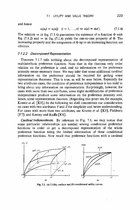
and hence
7.1 UTILITY AND VALUE THEORY
ui(ai) = u;(a;) (i = 1, ... , n) ¢> u(a) = u(a').
223
(7.1.4)
The relation => in Eq. (7.1.4) guarantees the existence of a function $ withEq. (7.1.2) and <= in Eq. (7.1.4) yields the one-to-one property of $. Theincreasing property and the uniqueness of $ up to an increasing function areobvious.
7.1.2.2 Decomposed Representation
Theorem 7.1.7 tells nothing about the decomposed representation ofmultiattribute preference function. Note that in the theorem only orderrelation on the preference is used, and no information on the preferenceintensity seems necessary there. We may infer that some additional cardinalinformation on the preference should be required for getting somerepresentation theorems. This is true, as will be seen below. Especially fortwo attributes cases, the condition of preference independence is too mild tobring about any information on representation, Surprisingly, however, forcases with more than two attributes, some slight modifications of preferenceindependence produce some information on the preference intensity and,hence, some representation theorem. (Regarding this point see, for example,Krantz et al. [K9].) In the following we shall concentrate our considerationon cases with two attributes Yand Z for simplicity and better understanding.For cases with more than two attributes, see Krantz et al. [K9], Fishburn[F7], and Keeney and Raiffa [K6].
CardinalIndependence. By reference to Fig. 7.1, we may notice thatsome particular relationships are needed among conditional preferencefunctions in order to get a decomposed representation of the wholepreference function using the limited information of these conditionalpreference functions. Now recall that preference functions with a cardinal
u(v, z)
u{y*, z*)
":------------"'-----yv'
(01
ulvlzlu(vlzl
(bl
Fig.7.1. (a) Utility surface and (b) conditional utility curves.

224 7 METHODOLOGY
(7.1.7)
(7.1.6)
measure are unique up to a positive affine transformation. In other words, apreference function U is equivalent to another preference function v ascardinal measure if
U = IY. + f3v for some IY. and f3 > 0. (7.1.5)
Consider a particular case in which all conditional preference functions overthe attribute Yare equivalent to each other independent of the level of Z,namely, all conditional preference functions u(', z) over Y become the same iftheir origins and units are set in common. More formally, let u(y Iz) be thenormalized conditional preference function over Yat z defined by
( Iu(y, z) - u(yo, z)
u Y z) = ---"--'---"----=-u(y*, z) - u(yO, z)
for given land y* E Y (yO and y* may be set respectively as the worst leveland the best level of 1', if any), for which we have u(yO Iz) = °and u(y* Iz) = 1for all z E Z. Then the special case under consideration requires that all thesenormalized conditional preference functions become identical with eachother regardless of the level z. Under such a circumstance, therefore, sincethese normalized conditional preference functions are not affected by thelevel z E Z, they can be delegated by u(y IZO). We define Ul(Y) = u(y IZO). Thenletting u(yo,ZO) = 0, we have
k1Ul(y) = u(y, ZO), k1 = u(y*, zO).
Henceforth, for convenience in this book we refer to this specialindependence condition on the conditional preference functions as thecardinal indpendence.
Definition 7.1.9 (Cardinal Independence)
The attribute Y is said to be cardinally independent of the attribute Z, if allconditional preference functions over Yare equivalent to each other ascardinal measure independently of the level of Z.
Theorem 7.1.8
The attributes Y and Z are cardinally independent of each other, if andonly if
u(y, z) = k1u1(y) + k1Ul(Z) + k12Ul(Y)Uz(Z)
Here, for (yO, ZO) and (y*, z*) such that (y*, ZO) » (y", z")(y", ZO), we normalize each preference function as
(1) u(l, ZO) = 0, u(y*, z*) = 1,(2) Ul(YO) = 0, Ul(Y*) = 1,(3) uz(ZO) = 0, Ul(Z*) = 1.
(7.1.8)
and (yO, z*) »

Then we have
7.1 UTILITY AND VALUE THEORY 225
(i) k 1 = U(y*, ZO),(ii) k2 = U(yO, z*),
(iii) k12 = 1 - k1 - k2 •
Proof It has been seen that if the attribute Yis cardinally independent ofZ, then Eq. (7.1.7) follows through the normalization Eq. (7.1.6) for eachconditional preference function over Y at every Z E Z and u(yO, ZO) = O.Similarly, if Z is cardinally independent of Y, then for U2(Z) := u(z IyO) with
u(ZIy) = (u(y, z) - u(y, ZO))/(u(y, z*) - u(y, ZO))
and u(yO, ZO) = 0, we have
(7.1.9)
Note here that from Eq. (7.1.6)
u(y,z) = u(yO,z) + [u(y*,z) - u(yO,Z)]Ul(y),
and similarly from (7.1.9)
u(y, z) = u(y, ZO) + [u(y, z*) - u(y, ZO)] U2(Z),
Hence, substituting Eq. (7.1.11) with y = y* into (7.1.10),
u(y, z) = k2u2(Z) + [k 1 + (1 - k1)1I2(Z) - k2I1iz)]u1(y)
= k11l](Y) + k2u2(Z) + (1 - k1 - k2)U1(Y)1I2(z).
The reverse is obvious.
(7.1.10)
(7.1.11)
As a particular case, with k 1 + k 2 = 1, we have an additive decomposition
(7.1.12)
Let us consider the geometric meaning for this case in more detail. Recallthat the cardinal independence condition admits the arbitrariness of both theorigin and the unit for each conditional preference function. If the preferencefunction u(y, z) has an additively decomposed representation [Eq. (7.1.12)],then it is easily seen that each conditional preference function over Y has acommon unit and leaves only a difference of origin. Conversely, if eachconditional preference function over Y has a common unit and leaves adifference of origin, then for all Y E Yand Z E Z
II(Y,z) = iX(Z) + u(y,ZO). (7.1.13)
Substituting u(yO, ZO) = 0 into Eq. (7.1.13), we have iX(Z) = u(yO, z), whence
u(y,z) = u(yO,z) + u(y,ZO). (7.1.14)
226 7 METHODOLOGY
Equation (7.1.14) yields Eq. (7.1.12). It should be noted here that if eachconditional preference function over Y has only the arbitrariness of origin,then the one over Z automatically has the same property.
The above discussion leads to the following theorem.
Definition 7.1.10 (Additive Independence)
The attributes Y and Z are said to be additive independent, if eachconditional preference function over either Y or Z has a common unit andleaves only the arbitrariness of origin.
Remark 7.1.9
As stated above, the condition of additive independence is symmetric,whereas the condition of cardinal independence is not so. Namely, even if Y iscardinally independent of Z, Z is not necessarily cardinally independent of Y.
Theorem 7.1.9
The attributes Yand Z are additive independent if and only if
u(y,z) = k1Ul(Y) + k2U2(Z).
Here, for (yO, ZO) and (y*, z*) such that (y*, z°»o. (yO, ZO) and (yO, z*) >-(yo, ZO), we normalize each preference function as
(1) u(yO, zo) = 0, u(y*, z*) = 1,(2) Ul(YO) = 0, Ul(Y*) = 1,(3) U2(ZO) = 0, U2(Z*) = 1.
Then we have
(i) k1 = u(y*, ZO),(ii) k2 = u(yO, z*),
(iii) k1 + k2 = 1.
Cardinal Independence in Decision Making under Risk. Now we shallconsider practical implications of the stated independence conditions. In thefollowing, we shall use the notation Y for representing the set of allprobability measures over Y, which also stands for the set of risky outcomesover Y. Recall that the expected preference principle by von Neumann andMorgenstern asserts that in decision making under risk there exists a utilityfunction such that
p >- q ¢>fu(y)dP(y) > fu(y) dQ(y).
where P(y) and Q(y) represent the probability distribution functionscorresponding to the risky outcomes p and q, respectively. Moreover, at'
7.1 UTILITY AND VALUE THEORY 227
important thing is that such a utility function is unique up to a positive affinetransformation. Note that, according to von Neumann-Morgenstern utilitytheory, utility functions that are equivalent to each other as cardinal measurereflect the same preference order over risky outcomes. Therefore, if theconditional preference over risky outcomes (Y,z) does not depend on thelevel z, then the conditional utility functions over Yare equivalent as cardinalmeasure independently of z. As a result, as long as we consider utilityfunctions in the sense of von Neumann-Morgenstern, the condition ofcardinal independence can be restated by a preference independence overrisky outcomes.
Definition 7.1.11 (Utility Independence)
The attribute Y is utility independent of another attribute Z, if thepreference over risky prospects (Y,z) does not depend on z; namely, if
(Vi,z") ~ (ji2,ZO) for some ZO ~ <.VI, z) ~ (j)2,z) for all z E Z,
where jil and ji2 are probability measures on Y.
Theorem 7.1.10
In decision making under risk, the overall utility function u(y, z) isdecomposable in the bilinear form in Theorem 7.1.8, if and only if Yand Zare utility independent of each other.
Remark 7.1.10
Fishburn and Keeney [F12] suggested for risky choices a condition calledthe generalized utility independence without restriction of the positiveness off3 in Eq. (7.1.5). Under the condition, we can get a more general multi-plicative representation. However, it will be seen later that this is included inthe representation form under the more general condition of interpolationindependence (Theorem 7.1.16).
As to the additive independence in decision making under risk, Eq. (7.1.5)yields the following expected utility for some risky alternative with theprobability distribution p(y,z)
Sy*s z*p(y,z)u(y, z) dy dz = SY*fz*p(y, Z)[IX(Z) + k1u1(y)] dy dz
yO zO yO zO
= i:Tf~*p(y,Z)dY}(Z)dZ
+f~Ti:*p(y, z) dz}IUl(Y) dy. (7.1.15)
228 7 METHODOLOGY
Note here that the terms J~~ p(y, z)dy and g~ p(y, z)dz denote the marginaldistribution of p(y, z) on Z and Y, respectively. In addition, it should be notedthat in Eq. (7.1.15) only the marginal distribution causes the difference ofexpected utility for risky alternatives. Now we have the following implicationof the additive independence in risky decisions.
Definition 7.1.12 (Additive Utility Independence)
In decision making under risk with two attributes Yand Z, Yand Z aresaid to be additive utility independent, if the preference over Y x Z is decidedby only the marginal distributions of the risky alternatives.
Theorem 7.1.11
In decision making under risk, the overall utility function u(y, z) isdecomposable in the additive form of Theorem 7.1.9, if and only if theattributes Yand Z are additive utility independent.
Cardinal Independence in Decision Making under Certainty. We haveseen through the above discussion that some cardinal information on thepreference is indispensable for additive or bilinear decomposition. How cansuch cardinal information under certain circumstances be elicited from thedecision maker? As a simple example, in particular, we assume the existenceof measurable value function defined in the preceding section.
Let y* be a nonempty subset of Y x Yand let >-* be a binary relation ony* reflecting a weak order of preference difference for >- on Y. We have seenin Theorem 7.1.4 that some appropriate conditions ensure a measurablevalue function u(·) such that if i >- y2 and y3 >- y4, then
yly2 >-* y3y4 <=> U(yl) _ U(y2) > U(y3) _ U(y4). (7.1.16)
In addition, this measurable value function is unique up to a positive affinetransformation; namely, two measurable value functions u and v areequivalent (i.e., reflect the same order >-*), if and only if there exist (f. andpositive psuch that
u= (f. + pv.
Therefore, it can be readily seen that the attribute Y is cardinally independentin the preference order >-* of the attribute Z, if and only if the conditionalorder of >-* on Yat z is not affectedby z; namely,
(i, ZO)(y2, ZO) >-* (y3,ZO)(y4, ZO) for some ZO E Z
= (yl,Z)(y2,Z)>-*(y3,Z)(y4,Z) forevery ZEZ. (7.1.17)
7.1 UTILIlY AND VALUE THEORY 229
In other words, this condition implies that the order of the preferencedifference over Y is not affected by the level of Z.
Definition 7.1.13 (Weak Difference Independencef
The attribute Y is said to be weak differenceindependent of the attribute Z,if, for any yl, yZ, y3, and y4 over Y, the relation (7.1.17) holds.
As a corollary of Theorem 7.1.8, we have the following theorem.
Theorem 7.1.12 t
In decision making under certainty with two attributes Yand Z, supposethat there exists a measurable value function u(y, z). Then, u(y, z) isdecomposable in the bilinear form of Theorem 7.1.8, if and only if theattributes Y and Z are preferentially independent and weak differenceindependent of each other.
Recall that, in Theorem 7.1.8, the additive decomposition is possible if andonly if k1 + kz = 1, where k1 = u(y*, ZO), kz = u(yO, z*), u(y*, z*) = 1,u(yO, ZO) = 0, (y*, ZO) >- (yO, z"), and (yO, z*) >- (yO, ZO). Since y*, yO, z*, and ZO
are introduced merely in order to define the unit and the origin, they can bearbitrarily chosen. Hence, letting some y1, yZ, z', and ZZ act for y*, yO, z*, andz", respectively,
k1 + kz = 1 '¢> u(yl, ZI) - u(yZ, ZI) = u(yl, ZZ) - u(yZ, ZZ),
which leads to the following theorem.
Theorem 7.1.13
The measurable value function u(y, z) is decomposable in the additive formof Theorem 7.1.9, if and only if, in addition to the assumptions of Theorem7.1.12, the following holds:
(yl, z l Xyz, ZI) """'*(yl, zZ)(yZ,ZZ) (7.1.18)
for arbitrarily chosen v',yZ E Yand ZI, ZZ E Z, such that
and
(7.1.19)
for some yO E Y. (7.1.20)
t Dyer and Sarin [D 10].I Theorems 7.1.12 and 7.1.13 from Dyer and Sarin [DlO].
230 7 METHODOLOGY
Remark 7.1.11
As a result of Theorem 7.1.13, it should be noted that if, under theassumption of weak difference independence, Eq. (7.1.18) holds for somei,y2 E Yand some z1,z2 E Z satisfying Eqs. (7.1.19) and (7.1.20), then Eq.(7.1.18) holds for all y1, y2 E Y and all z1, Z2 E Z satisfying Eqs. (7.1.19) and(7.1.20). In fact, the additive decomposition implies each conditionalmeasurable function has a common unit, and hence the preference differencebetween two arbitrarily given points over Y x z is identical independentlyof z.
Without the assumption of weak difference independence, the additivedecomposition can be obtained as follows. Recall that the additiveindependence implies that all conditional value functions over each attributehave a common unit and only their origins vary depending on levels ofanother attribute. This implies, in other words, that the difference of theconditional preference function u(y Iz) between the points (y1,z) and (y2,z) isnot affected by z, whereby according to Eq. (7.1.16), the difference of theintensity of the conditional preference over Y does not depend on the levelofZ.
Definition 7.1.14 (Difference Independencef
The attribute Y is said to be difference independent of Z, if for all yl, y2 E Ysuch that (yl, ZO) ~ (y2,ZO) for some ZO E Z
(/, Z)(y2, z) -* (/, zO)(f, ZO) for all z E Z.
Theorem 7.1.14
Assume that a measurable value function u(y,z) exists for the givenpreference over Y x Z. Then u(y, z) is decomposable in the additive form ifand only if the attributes Y and Z are preferentially independent of eachother and Yis difference independent of Z.
Conditional measurable value functions may be calibrated by somemethods such as the direct rating method or the direct midpoint method(Fishburn [F6J). Once some conditional measurable value functions areassessed, the weak difference independence condition can be easily checkedby comparing their normalized function forms.
However, in cases that the assessment of conditional measurable valuefunction is not easy, or trade-off between one attribute and another can berelatively easily made, the trade-off can be used for eliciting cardinalinformation on the preference for the additive decomposition.
t Dyer and Sarin [D10].

7.1 UTILITY AND VALUE THEORY
z
Z3 I----....---~
z2 t----~--~M---~K
z1 t-----+----~r__--....;lI...:
'--__..........JL.....-__~ __L y
yl y2 y3
Fig. 7.2. Thomsen condition.
231
The additive independence condition can be restated in connection withthe trade-off between Yand Z as follows. In Fig. 7.2, since the points A and Bare on an indifference curve 11, the difference of the conditional preferenceover Ybetween i and yl at z = z' equals that of the conditional preferenceover Z between Z1 and Zl at y = i. These differences of conditionalpreferences may be represented by Aut and Aui in terms of measurable valuefunction. A similar argument can be made for the points C and D on theindifference curve 12 , Now the additive independence condition asserts thatthe difference Aut of the conditional preference over Y between i and yl isnot affected by the level of Z. The same is true for other differences ofconditional preferences. Therefore, the difference of conditional preferencebetween the points P and Q can be represented by Aut + Aui for theattribute Yand Aui + Au~ for the attribute Z. In view of that Aut = Aui andAui = Au~, it finally follows that the point P should be indifferent to thepoint Q. This observation leads to the well-known Thomsen condition.
Definition 7.1.15 (Thomsen Conditionv
A weakly ordered set (Y x Z, >-)is said to satisfy the Thomsen condition, iffor any yt, y2, y3 E Yand Zt, Z2,Z3 E Z,
(i,Zl) ~ (yl,Z1)} (1 3 3 1)(y2,Z3) ~ (y3,Zl) => y,z ) ~ (y ,z .
t Kranz et al. [K9].

232
Remark 7.1.12
7 METHODOLOGY
The conditions of preference independence and Thomsen give sufficientpower for the additive decomposability of value functions. However, someadditional conditions are required for ensuring the existence of such anadditively decomposed value function.
Definition 7.1.16 (Solvability Condition)
A weakly ordered set (Y x Z, >-)is said to satisfy the solvability conditionif there exists some y E Ysuch that
(y, z*) '" (y', z*),
Definition 7.1.17 (Archimedean Condition)
A weakly ordered set (Y x Z, >-) is said to satisfy the Archimedeancondition, if the following holds. If, for any z, Z E Z, the sequence{i, y2, ... , y\ ...} such that (y\ z) '" (/+ 1, z) (Vk) is bounded, then it isfinite.
Remark 7.1.13
Recall that the set of real numbers satisfies the continuity property and hasa subset countable and dense in it in connection with the structure of orderand addition. The condition of solvability and that of Archimedean ensuresimilar properties for (Y x Z, >-). (For details, see Krantz et al. [K9].)
Theorem 7.1.15 t
Suppose the following conditions hold for (Y x Z, >-):
(Cl) >- is a weak order:(C2) the attributes Yand Z are mutually preferentially independent;(C3) the Thomsen condition holds:(C4) the solvability condition holds;(C5) the Archimedean condition holds.
Then there exists a value function u: Yx Z --+ R 1 which is decomposable inan additive form.
t Kranz et al. [K9].

7.1 UTILITY AND VALUE THEORY 233
Proof Since the precise proof is complicated, we shall sketch an outline ofthe proofs. Given y, z, y*, and z*, let (y), tI(z)be solutions such that
(y*, (y» ~ (y, z*), (tI(z), z*) ~ (y*, z),
and let v' 0 yZ E Ybe a solution to«y! 0 yZ), z*) ~ (yt, (yZ».
A key idea to the proofis that for any bounded subset of (Y x Z, »), (Y,»Y.0)is of additive structure; i.e., there exists a function u, unique up to a positiveaffine transformation such that
y' »y y2 ¢:> u,(y,) > u,(yZ)
u,(y! 0 yZ) = u,(y!) + u1(yZ).
Then, the preference independence condition yields
(y', z'»> (yZ, ZZ) ¢:> y' 0 tI(z'»>y yZ 0 tI(ZZ),
and hence letting uz(z) = u,(tI(z»
(i, Z1) » (y2,Z2) ¢:> u,(y!) + uz(z') > u,(yZ) + uiz2).
The theorem is established by extending u, and Uz to the whole space(Y x Z, »).
For the additive decomposition of value functions, several methods havebeen developed for testing the Thomsen condition and the assessment of thevalue function simultaneously. We shall introduce briefly a method called thelock step method based on the above proof (Keeney and Raiffa [K6]) (Fig.7.3).
(1) Define yO and ZO as the least preferred level of Yand Z, respectively.Set u(yO, ZO) = Ut(YO) = uz{ZO) = O.
(2) Take y' in such a way that (y', z") » (yO, ZO) and set U1(Y!) = 1.(3) Find z' such that (yO,Z1) ~ (y!,zo) (due to the solvability condition)
and set uz(z') = 1.(4) Find yZ and Z2 such that (yZ, ZO) ~ (y!, Z1) ~ (yO, Z2) and set U1(y2) =
U2(ZZ) = 2.(5) Check whether or not (y!, Z2) ~ (yZ, Z1), which is a part of the
Thomsen condition. If the condition holds, go to the next step. Otherwise, wecan not have the additive decomposition.
(6) Find land Z3 such that (l, z") ~ (y2,z ') ~ (y', Z2) ~ (yO, Z3) and setu1(l) = uz(Z3) = 3.
(7) Check whether or not (y3, Z1) ~ (y2,ZZ) ~ (y1,Z3).(S) Continue the same process for some appropriate number of sample
points.(9) Decide the function forms of u1(y) and uz(z) by some appropriate
curve fitting method and set u(y, z) = U1(y) + uz(z).
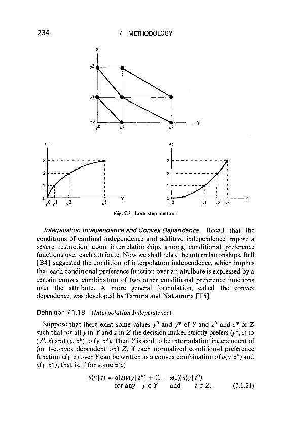
234 7 METHODOLOGY
z
Zl ...--....-----~
zO L.-_----.:__-----.:~--- yyO
zl z2 z3
L-L..-..: ...;..._ y o ~.-..=;---'-----'-----''-- ZzO
Fij:. 7.3. Lock step method.
Interpolation Independence and Convex Dependence. Recall that theconditions of cardinal independence and additive independence impose asevere restriction upon interrelationships among conditional preferencefunctions over each attribute. Now we shall relax the interrelationships. Bell[B4] suggested the condition of interpolation independence, which impliesthat each conditional preference function over an attribute is expressed by acertain convex combination of two other conditional preference functionsover the attribute. A more general formulation, called the convexdependence, was developed by Tamura and Nakamura [T5].
Definition 7.1.18 (Interpolation Independence)
Suppose that there exist some values yO and y* of Y and ZO and z* of Zsuch that for all yin Yand z in Z the decision maker strictly prefers (y*, z) to(yO, z) and (y, z*) to (y, ZO). Then Y is said to be interpolation independent of(or 1-convex dependent on) Z, if each normalized conditional preferencefunction u(y Iz) over Y can be written as a convex combination of u(y Iz'') andu(y Iz*); that is, if for some ce(z)
u(y Iz) = O!(z)u(y Iz*) + (1 - O!(z»u(y IZO)for any y E Y and z E Z. (7.1.21)
Remark 7.1.14
7.1 UTILITY AND VALUE THEORY 235
As is readily seen, the notion of interpolation independence includesseveral other independence conditions as special cases. For example, ifu(y IZO) = u(y Iz*) and u(z IyO) = u(z Iy*), the condition that Y isinterpolation independent of Z reduces to the condition that Y is cardinallyindependent of Z.
Note that, conversely, if Y is cardinally independent of Z, then not only isY interpolation independent of Z, but Z is also interpolation independentof Y.
Theorem 7.1.16 t
The attributes Yand Z are interpolation independent of each other if andonly if
u(y, z) = k[u(y IZO) + k2u(z IyO) - ku(y IzO)u(z IyO)+ (k - kl)U(Y IZO)u(z Iy*) + (k - k2)u(y Iz*)u(z IyO)+ (1 - k)u(y Iz*)u(z Iy*), (7.1.22)
where k1 = u(y*, ZO), k2 = u(yO, z*), and k is an independent constant.
Proof
if Suppose that Eq. (7.1.22) holds. Then Eq. (7.1.22) yields
u(yO,z) = k2 u(z l yo) and u(y*,z) = k1 + (1- kdu(zIY*),
because u(yO Iz) = 0 and u(y* Iz) = 1 for any Z E Z. Hence,
u(y Iz) = (u(y, z) - u(yO, z))/(u(y*, z) - u(yO, z))
{k 1 - ku(z IyO) + (k - k1)u(zIy*)}u(y IZO)
+ {(k - k2)u(z IyO) + (1 - k)u(z Iy*)} u(y Iz*)
k1 + (1 - k1)u(zly*) - k2u(zIYO)
which is of the form of Eq. (7.1.21) showing that Y is interpolationindependent of Z. Similarly, it can be shown that Z is interpolationindependent of Y.
only if Suppose that Yand Z are mutually interpolation independent.For a special case where u(y IZO) = u(y Iz*) and u(zIyO) = u(zIy*), thecondition of Yand Z being mutually interpolation independent implies thatYand Z are mutually cardinally independent, which leads to Eq. (7.1.22)with k = k2 . Therefore, for the remainder of the proof, we assume thatu(y IZO) is not identical to u(y Iz*) and that u(zIyO) is not identical to u(zIy*).
t Bell [B4].

236 7 METHODOLOGY
From the definition of the normalized conditional preference functionover Ywith u(y*, ZO) = k., and u(Y°, z*) = k2 [cf. Eq. (7.1.6)J, we have
u(y,z) = k2u(z IyO) + [k 1 - k2u(z IyO) + (1 - k1)u(z Iy*)]u(y Iz).
from which the condition that Y be interpolation independent of Z produces
u(y,z) = k2u(z IyO) + G2(Z)[1X2(Z)U(Y Iz*) + (1 - 1X2(Z»U(Y IZO)], (7.1.23)
where
G2(z) = k1 - k2u(zIyO) + (1 - k1)u(zIy*).
Similarly, from the condition that Z be interpolation independent of Y,
u(y, z) = k1u(YlzO) + G1(Y)[1X1(y)u(zIY*) + (1 - 1X1(y»u(zIYO)], (7.1.24)
where
G1(y) = k2 - k1u(YlzO) + (1 - k2)u(ylz*).
Fixing z at some z :f: ZO in Eqs. (7.1.23) and (7.1.24), we may see that forsome constants Clo C2, and C3 .
G1(Y)1X1(Y) = Cl + C2 U(Y IZO) + C3U(Y Iz*).
Here Cl = 0 and C2 + C3 = 1 - k1 because G1(yO) = k2, G1(y*) = 1·- kb
1X1(YO) = 0, and 1X1(Y*) = 1. Finally, using a constant Cinstead of C2'
G1(Y)1X1(Y) = cu(ylzO) + (1- k1 - c)u(ylz*).
Similarly, for some constant d,
G2(Z)1X2(Z) = du(zIyO) + (1 - k2 - d)u(zIy*).
Substituting them into Eqs. (7.1.23)and (7.1.24),
(k1 - k2 + C - d)(u(YlzO) - u(Ylz*)Xu(zIYO) - u(zly*» = 0,
whence
k1 + C = k2 + d.
Substituting GiZ)1X2(Z) with k = k2 + d into Eq. (7.1.23), we finally have
u(Y,z) = k2u(z IyO) + [k1 - k2u(zIYO) + (1 - k1)U(zly*)]u(YlzO)
+ (u(y Iz*) - u(y IzO»[(k - k2)u(z IyO) + (1 - k)u(zIy*)]
= k1u(yIZO) + k2u(zIYO) - ku(YlzO)u(zIYO)
+ (k - kJly(y IZO)u(z Iy*) + (k - k2)u(y Iz*)u(z IyO)
+ (1 - k)u(y Iz*)u(z Iy*).

7.1 UTILITY AND VALUE THEORY 237
Remark 7.1.15
The decomposed representation of Theorem 7.1.16 clearly includes otherrepresentations stated above as special cases. It reduces to the one underbilateral independence (Fishburn [F9]) if (k1 + k2 - l)k = k1k2 , and to theone under the generalized utility independence if k = 1. Further, if u(y IZO) =u(y Iz*) and u(z IyO) = u(z Iy*), it reduces to the one under the cardinalindependence, and in addition, if k1 + k 2 = 1, the additive decompositionresults.
7.1.2.3 Assessmentof Multiattribute Preference Functions
Although we introduced some methods for assessing some of particularmultiattribute utility functions, we shall summarize here an effective methodbased on conditional preference functions using a graphic display terminal ofcomputer. Consider cases with two attributes Yand Z for simplicity.
(1) Set the best level y* and z* and the worst level yO and ZO for attributesYand Z, respectively.
(2) Assess some representative conditional preference functions over eachattribute in the normalized form, i.e., in such a way that u(y° Iz) = 0 andu(y* Iz) = 1 for any Z E Z and similarly for u(z Iy).
(3) Depict graphs of the normalized conditional preference functionsover each attribute on the graphic display.
(4) If all normalized conditional preference functions over Yareperceived identical, then it may be considered that the attribute Y iscardinally independent of Z. In addition, if Z is also cardinally independentof Y, then we will have in general the bilinear utility function. In this case,assess the scale constants k1 and k2 by asking the trade-off between Yand Z;i.e.,in risky choices, ask for the decision maker probabilities C( and [3 such that
(y*, ZO) ~ [(y*, z*), (yO, ZO): c(, 1 - C(]
(yO, z*) ~ [(y*, z*), (yO, ZO): [3,1 - [3],
from which k1 = C( and k2 = [3. If k1 + k2 = 1, then the utility functionreduces to the additive form, otherwise it reduces to the bilinear form, inwhich the constant k is decided by solving 1 + k = (1 + kk 1X1+ kk 2 ) .
(5) If only Yis cardinally independent of Z, and if Z is not of Y, then Z isinterpolation independent of Y(see Remark 7.1.14), and hence both Y and Zare interpolation independent of each other. Go to step (7).Ifneither Y nor Zis cardinally independent of the other, go to step (6) for the check ofinterpolation independence.

238
(6) Set
7 METHODOLOGY
Ul(y : «) = ()(U(y Iz*) + (1 - ()()U(y IZO).
For a sample level Z, take y appropriately (for example, y = (yO + y*)/2).Find a solution &to the following equation
u(Y, z) = ()(u(y Iz*) + (1 - ()()u(y IZO).
Compare the utility curves of u(y Iz) and Ul(y : Ii). If we observe that thesetwo curves are identical for several levels of Z, then Y may be consideredto be interpolation independent of Z. Check for the conditional preferencefunctions over Z in a similar way. Go to step (7) if both Y and Z areinterpolation independent of each other, otherwise some other decomposedrepresentation would be possible (for example, nth convex dependencedecomposition, Tamura and Nakamura [T5]).
(7) Assess the scale constants k 1 and k2 in the similar way to step (4).Decide k directly from the utility at some representative point.
Due to recent remarkable developments of micro computers, theassessment method stated above is expected to be useful for practicalproblems in an interactive way with ease. For cases with more than twoattributes, the consistency check of trade-off constants may be a problem. Asuggestion using Saaty's method for cardinal ranking (Saaty [SI]) is seen inSawaragi et al. [S5].
7.1.3 Discussions
In the preceding subsections, we have introduced some of the represent-ative theorems regarding existence, uniqueness, and decomposed repre-sentation for multiattribute preference functions. These theorems are of anormative theory based on some assumptions. In applying them in practicalproblems, therefore, it is meaningful to check the properness of theseassumptions from some viewpoint of behavioral science and to know thelimits of the theorems.
7.1.3.1 A//ais Paradox
One of the most famous cnticisms for von Neumann-Morgensternexpected utility theory was claimed by Allais (see, for example, Allais andHagen [AI]). We shall explain it using the example given by Kahneman andTversky [KI]:
Consider a pair of lotteries L 1 with a gain of 3000 for sure andL2 = [4000,0: 0.80, 0.20], and another pair of L3 = [3000,0: 0.25, 0.75]

7.1 UTILITY AND VALUE THEORY 239
and L 4 = [4000,0: 0.20, 0.80]. According to an experiment by Kahnemanand Tversky, many respondents preferred L 1 for the first pair and L4 for thesecond pair. Note that their preferences are not consistent with the vonNeumann-Morgenstern expected utility theory. In fact, for the preferenceover the first pair, a von Neumann-Morgenstern utility function u(·) withu(O) = 0 prod uces
u(3000) = 1.0u(3000) + O.Ou(O) > 0.8u(4000) + 0.2u(0)
= 0.8u(4000). (7.1.25)
On the other hand, for the preference over the second pair,
0.2u(4000) = 0.2u(4000) + 0.8u(0) > 0.25u(3000) + 0.75u(0)
= 0.25u(3000) (7.1.26)
We have from Eq. (7.1.25) u(3000)/u(4000) > 0.8, whereas from Eq. (7.1.26)u(3000)/u(4000) < 0.8, which lead to a contradiction.
Now let us consider a reason why such a contradiction for the vonNeumann-Morgenstern utility function arise. To this end, observe that thelottery L 3 can be regarded as a compound lottery [L,, 0: 0.25,0.75J and alsoL 4 as [L z, 0: 0.25,0.75J. The independence condition C2 of Theorem 7.1.6implies that if we prefer L 1 to L z, then we must prefer L 3 to L4 , which isviolated by the preference stated above. In many other reports also (see, forexample, Allais and Hagen [A1J and Machina [M1J), such a violation of theindependence condition has been observed.
Kahneman and Tversky considered that the stated preferenceincompatible with the independence condition of von Neuman-Morgensternexpected utility theory is caused from the certainty effect, which implies thatpeople overweight outcomes that are considered certain, relative to outcomeswhich are merely probable.
Another effect violating the independence condition is observed by thefollowing example. Consider a pair of lotteries L 5 = [3000, 0: 0.90,0.10Jand L 6 = [6000,0: 0.45, 0.55J, and L 7 = [3000,0: 0.02, 0.98J and L 8 =[6000,0: om, 0.99]. Most people would prefer L 5 to L 6 for the first pair,because although both L 5 and L 6 have the same expected monetary value,the probability of winning for L 5 is much larger than that for L6 • For thesecond, on the other hand, probabilities of winning for the lotteries are bothminuscule. In this situation where winning is not almost probable, mostpeople would prefer L 8 with a large gain to L 7 • This effect suggested byKahneman and Tversky is called the get-rich-quick effect in the literature(Sakai [S2J). Regarding L 7 as a compound lottery [L 5 , 0: 1/450,449/450Jand L 8 as [L6 , 0: 1/450,449/450J, we may see that the preceding exampleviolates the independence condition of Theorem 7.1.6.

240 7 METHODOLOGY
1------------------ ----
oFi~. 7.4. Weighting function for probability.
p
Observing further effects that violate the expected utility theory, say, thereflection effectt and the isolation effect ~ Kahneman and Tversky [K1]suggested a weighted value function model (prospect theory) for a simpleprobability measure p over Y
u(P) = L n(p(y»u(y),yEY
where n(p) is a weighting function for probability with a property of Fig. 7.4.It has been reported that such a modification of the expected utilityovercomes several drawbacks in the von Neumann-Morgenstern expectedutility theory. For more details, see the original work by Kahneman andTversy [Kl].
7.1.3.2 Group Decisions and Equity
In group decisions, the well-known Arrow's general impossibility theorem([A2], [F8]) asserts that it is impossible in a general sense (under Arrow's five
t The preference tendency is called the reflection effect if we 0 bserve the preference over a pairof risky alternatives reverses when all the outcome values are reversed in sign. For example, therisk aversion on the positive domain leads to the risk prone in the negative domain.
l A risky alternative can be reconsidered as a compound lottery in various ways; sometimes apreference changes over ways of decomposition. This phenomenon is called the isolation effect.
7.1 UTILITY AND VALUE THEORY 241
conditions) to aggregate individuals' preference orders into a social one.tNumerous researches have tried to overcome the difficultypointed by Arrow,but it is considered to be essentially impossible to get out of the stateddilemma. The most controversial subject is directed towards theindependence of irrelevant alternatives which is imposed in order to avoidthe measurability of preferences. It has been known, however, that even ifeach individual value (utility) can be evaluated quantitatively, there does notexist any social choice function without interpersonal comparison of values(utilities) (Sen [S7]).
A group Bayesian approach tries to find a group utility function byregarding the group (society) as a man having rationality consistent with theexpected utility theory (Raiffa [Rl]). Harsanyi [H4] showed that if both theindividuals and the group satisfy the conditions of Theorem 7.1.6, and if thegroup is indifferent between two risky alternatives whenever all individualsare indifferent, then the group utility function should be a linear combinationof individual utilities. Note here that such a linearity of the group utilityfunction is mainly due to the independence condition of Theorem 7.1.6. Infact, the proof by Harsanyi proceeds as follows. Under the assumption, thegroup utility function is a function of the expected utilities of individuals.The group utility function based upon Theorem 7.1.6 is a linear functionover the set of risky prospects of individual expected utilities. We shall showthis in more detail as follows. Suppose that, for a risky alternative P, eachindividual i has an expected utility Ui' Hence, we identify P as a prospect(Ub .•. , un)' Similarly, identify 0 as (0, ... ,0). Let Q be an uncertainprospect [P, 0: a, 1 - ct.]. Then clearly, Q = «P + (1 - ct.)O. According toTheorem 7.1.5, u(Q) = ct.u(P) + (1 - CI.)u(O), whereas u(Q) = u(ct.u 1, ••• , rY.un),u(O) = u(O, ... ,0) = °and u(P) = u(ub ..• , un), which leads to the first order
t Define a social choice function F by a functional relationship between the tuple of individualpreference (Pi, ... , P") and the social preference P; namely, P = F(p l, ... , PO). Arrow's generalimpossibility theorem says that under the assumption that there are at least two persons in thegroup and three alternatives, there is no social choice function satisfying the following fiveconditions:
(CI) The social preference P is a weak order.(C2) The domain of F must include all possible combinations of individual orderings
(unrestricted domain).(C3) For any pair x, x' in X, if xp1x' for all i, then xPx' (Pareto principle).(C4) Let P and P' be the social binary relations determined by F corresponding, respectively,
to two sets of individual preferences, (Pi, ... , P") and (pI', ... , PO'). If for all pairs of alternativesx, x' in a subset S of X, xPx' if and only if xP'x' for all i, then the greatest set of S with respect toP is identical to the one with respect to P' (independence of irrelevant alternatives).
(CS) There is no individual i such that xpix' implies that xPx' for every pair of elements x, x'in X (nondictatorship).
242 7 METHODOLOGY
homogenuity of u(U1> ... , Un) for 0 ~ a ~ 1. In addition, similar argumentsfor 0 = «R + (1 - a)P with R = (kul , ... , kUn), where k = 1 - Y]« andP = as + (1 - a)O with S = (kul> ... , kUn), where k = III>: yield the firstorder homogenuity of U(UI, ... , un) for k < 0 and k > 1, respectively. Theadditivity of U(Ul>"" un) follows immediately by considering a prospectS, = (0, ... , 1, ... ,0) (i = 1, ... , n) and T = [S I' ... , S; : lin, ... , lin].
We have seen that the independence condition of Theorem 7.1.6 plays akey role in deriving the linear group utility function via its linearity overuncertain prospect. However, Diamond [05] criticized this point. Let usconsider a problem with two individuals and two specific alternatives. Letthe alternative A be (UI = 1, U2 = 0) for sure and B (u[ = 0, U2 = 1)for sure.Unless we discriminate two individuals, the group should be indifferentbetween A and B. Now mix these two alternatives with the probability 0.5;that is, C = [A, A : 0.5, 0.5] and D = [A, B : 0.5, 0.5]. According to theindependence condition (in fact, according to a weaker condition called thesure thing principle t ), the group should be indifferent between C and D as longas A is indifferent to B. However, D seems more preferable to C in the sensethat in D both individuals have a possibility getting the prize, whereas in Cthe second person has no possibility getting the prize. Therefore, Diamondclaimed the group does not accept the expected utility theory.
In addition, Keeney [K4] pointed out that as long as the group 'utilityfunction is viewed as a function of individual expected utilities, it can notnecessarily take equity into account. For example, consider a problem withtwo individuals and two alternatives: the alternative P results in either(u[ = 1, U2 = 0) with probability one-half or (Ul = 0, U2 = 1) with prob-ability one-half. The alternative Q yields either (Ul = 1, U2 = 1) or(Ul = 0, U2 = 0), each with probability one-half. For each alternative, bothindividual expected utilities are 0.5, whence the linear group utility functiondoes not distinguish Q from P. However, from the viewpoint of equity, Qseems more preferable to P. This phenomenon may be considered a naturalresult from the fact that the group utility function as a function of individualexpected utilities is caused from an individualism in the sense that the groupis indifferent between two alternatives whenever all individuals are indifferentbetween them.
As is readily seen in the above discussion, it is hard to construct a grouputility function consistent with the expected utility theory and equity. Sen[S7] proposed that the social welfare function should depend not only on themean value of individual utilities but also on some measure of inequality(dispersion) in these individual utilities. Based on a similar idea, Nakayama
t For any p, q E Y, P - q => rxp + (1 - rx)r - «q + (I - rx)r for any r E Yand rx E (0, 1).

7.1 UTILITY AND VALUE THEORY 243
et al. [N 10J suggested the extended contributive rule (ECR) method bycombining the utilitarian index (linear combination of individual utilities)and a certain egalitarian index (variance of individual utilities), whose aim isto help mutual understanding of the group members toward a consensusrather than to get a social welfare index. Some kinds of utility functions thatincorporate equity are discussed in Keeney [K5J, Bodily [B5J and others. Asto group decisions in terms of parametric domination structures, see Taninoet al, [T12, T13J, and from a viewpoint of fuzzy set theory, see Tanino [T8].
7.1.3.3 Measurability of von Neumann-Morgenstern Utility Function
It is readily seen that the measurability of von Neumann- Morgersternutility functions strongly depends on the independence condition of Theorem7.1.5. From a viewpoint of behavioral science, however, we have observedthat the independence condition may be violated in many practical cases,where a sure prospect cannot necessarily be considered an uncertain prospectwith the probability one. Therefore, a utility function obtained by somemeasurement methods based on the certainty equivalent does not necessarilyreflect the preference correctly. More strongly, several researchers such asArrow [A3J, Baumol [B2J, Luce and Raiffa [L12J, and Dyer and Sarin [D9Jargued that von Neumann-Morgenstern utility functions do not measure theintensity of preference, though they evaluate the decision maker's attitudetoward risk. Recently, some trials of evaluating the preference intensity andthe risk attitude separately have been reported (Dyer and Sarin [DlOJ andSarin [S4J). In the previous section, we discussed a direct measurement ofpreference intensity and decomposed representation of measurable multi-attribute value functions.
7.1.3.4 Utility Functions Nonlinear in the Probability
We may see that the expected utility theory by von Neumann-Morgenstern is in a sense a linear model for the preference in risky choices.Of course, the real world is generally nonlinear. It depends on thenonlinearity whether or not the expected utility theory fits to the reality as afirst-order approximation. It would still remain valid for many practicalproblems keeping the stated limits in mind. Finally, we would like to mentionthat some devices for expected utility theory without the independencecondition have been developed recently (Fishburn [FlO, FllJ and Machina[MlJ), which are nonlinear in probability while keeping its measurability.For a review of recent developments of utility and value theory, see Farquhar[F3J.
244 7 METHODOLOGY
7.2 Stochastic Dominance
We have observed in the previous sections that the expected utility theoryplays a major role in risky decision making problems, while at the same time,there are some difficulties in assessing utility functions. The theory ofstochastic dominance has been developed for ranking risky alternativeswithout a complete knowledge on the utility function.
In the following, we suppose that our risky decisions follow the expectedutility theory by von Neumann-Morgenstern, but we know only partialinformation on the utility function of the decision maker. For simplicity, weidentify risky alternatives as cumulative probability distributions over apositive scalar attribute Y. Hence, for a risky alternative F, the expectedutility can be represented by
E(u, F) = IX) u(y)dF(y).
Definition 7.2.1
Consider utility functions that are bounded and appropriately smooth on[0, co). Let u', u", and u" denote the first, second, and third derivatives of theutility function u, respectively. Then the classes of utility functions IJlt 10 IJlt 2,
and IJlt 3 are defined as
(i) 1Jlt 1 := {ulu E C', u'(y) > 0, Vy E [0, CD)}.(ii) 1Jlt 2 := {ulu E e2, u E OU 1o u"(y) < 0, Vy E [0, CD)}.
(iii) 1Jlt3 : = {ulu E e3, u E 1Jlt 2 , u"'(y) > 0, Vy E [0, CD)}.
Remark 7.2.1
As is readily recognized, OU1 is the class of utility functions for which thedecision maker's preference is strictly increasing over outcomes. Further-more, IJlt 2 is the class of utility functions which are of IJlt 1 and risk averse.Finally, it is readily seen that decreasing risk averse utility functions belongto the class IJlt 3 .
Definition 7.2.2 (Stochastic Domination)
For i = 1,2,3,
F >;G if and only if E(u,F) > E(u, G), Vu E 1Jlt;.
We refer to >1 as the first-degree stochastic dominance (FSD) to >2 assecond-degree stochastic dominance (SSD) and >3 as third-degree stochasticdominance (TSD).

7.2 STOCHASTIC DOMINANCE 245
These domination relationships induce some kinds of partial orderingsover risky prospects. Therefore, although stochastic dominance may not, ingeneral be expected, to lead to the best alternative by itself, it may be helpfulto narrow down the alternative set.
Definition 7.2.3
Let f!lJ be the set of all right-continuous distribution functions withF(O) = O. For each FE fYJ, we define P as
F1(y) := F(y),
p+ 1:= J:P(y)dy, y E [0, 00).
Remark 7.2.2
The right continuity of F and G of fYJ implies that F 2 t= G2 when F t= G.Therefore, F = G follows whenever F" = G" for some n ~ 2.
Denote by G(y);::: F(y), Vy E [0,00) that G(y) ~ F(y), vv E [0,00) andG(y) > F(y) for at least some interval of [0, 00). Then, the first two parts of thefollowing theorem are due to Hadar and Russell [H1], and the last part isdue to Whitmore [WlOJ, (See also Fishburn and Vickson [F13].)
Theorem 7.2.1
The following hold:
(i) F >1 G ¢> G1(y) 2:: F1(y) for all y E [0, 00),(ii) F >2 G ¢> G2(y) 2:: F 2(y) for all y E [0, 00),
(iii) F >3 G ¢> /IF ~ /lG and G3(y) 2:: F 3(y) for all y E [0, 00),
where /IF denotes the mean value of F given by
/IF := f) y dF(y).
Proof Let D i = r - Gi (i = 1,2,3). Then since u(y) is bounded over[0,00),
E(u, F) - E(u, G) = {<Xl u(y) dD1(y)
= [u(y)D1(y)JO' _ {<Xl u'(y) dD 2(y)
= _{<Xl u'(y) dD 2(y).
from which the part <= for i = 1 is clear.

246 7 METHODOLOGY
The part = for i = 1 is established by leading a contradiction for a utilityfunction
u( ) = {ocexp[oc- 1(y- Yo)], for y ~ Yo,
Y oc + {I - exp[-oc(y - yo)]}/oc, for y ~ Yo,
if there exists Yo E [0, (0) such that F(y) ~ G(y) for y ~ Yo' and F(y) ~ G(y)for Yo ~ y.
Similarly, setting di) = diu/dyi, the part <= for i = 2 and 3 follows from
{"u(i-1)(y)dD i(y) = [u(i-1)(y)Di(y)]O' _ L"ou(i)(y)dDi + 1(y)
= -f) u(i)(y) dDi+1(y),
because for distributions F and G with finite mean values, Di(y) (i = 1,2) isfinite, and limc., co u(i)(y) = 0 (i = 1,2) is due to the monotonicalinceasingness and boundedness from above. In addition, = is derived in asimilar fashion by a contradiction using a utility function for >2
u(y) = - 0/o(2) exp[- oc(y - Yo)],
and for >3
y ~ Yo
y > Yo·
The necessity of IlF ~ IlG for >3 is obtained by a contradiction using a utilityfunction
u(y) = ky - 1 + exp[-ky],
which yields E(u, F) = -1 + kllF + o(k) where o(k)/k ~ 0 as kW. Formore details, see Fishburn and Vickson [F13].
Remark 7.2.3
Theorem 7.2.1 implies that if the cumulative distribution F is pointwisesmaller than G, then F is preferred to G in terms of the expected utilities aslong as the decision maker's preference is monotonically increasing overoutcomes (Fig. 7.5). However, in the case of F and G intersecting at a point,>1 gives no information on the domination between F and G. In such a case,if F 2 is pointwise smaller than G2
, then F is preferred to G in terms ofexpected utilities as long as the decision maker's preference is monotonically

7.2 STOCHASTIC DOMINANCE
_~ L.--_ X
Fi~. 7.5. F >1 G.
247
increasing over outcomes and risk averse (Fig. 7.6). Finally, in the case of F Z
and GZ intersecting at a point, if the decision maker's preference is decreasingrisk averse, we have a domination between F and G by checking each meanvalue together with F3 and G3
•
Remark 7.2.4
As is well known, EV-dominance, for which alternatives with largerexpected value and smaller variance are preferred, cannot be necessarilyadequate for decision problems, if we take the preference of the decisionmaker into account. (See,for example, Keeney and Raiffa [K6].) Moreover, ifIlF = Ila, then F >z G (F >3 G) implies (fF < (fa (resp. (fF ~ (fa). Clearly,IlF = Ila and F >1 G are inconsistent. On the other hand, if IlF > Ila, thenF > i G (i = 1,2,3) is neither necessary nor sufficient for (fF ~ (fa. In view of
t
L",.:::;~:::::::"_---_-1-x
Fi~. 7.6. F >2 G.
248 7 METHODOLOGY
these facts, stochastic dominance seems to be sufficiently adequate forreducing the alternative set in the light of decision maker's preference.
7.2.1 Multivariate Stochastic Dominance
Now we consider stochastic dominance for decision problems withmultiple attributes, in particular, with two attributes Y x Z for simplicity.
Definition 7.2.4 (Multivariate Risk Aversion)t
If for any Y1' Yz, Z1' and Z2 with Y1 < Yz and Z1 < Z2 a decision makerprefers the risky alternative which gives an even chance for (Yh Z2) or (Y2, z1)to the one which gives an even chance for (Y1' Z1) or (Y2' Z2), then hispreference is said to be multivariate risk averse.
Lemma 7.2.1 t
Let the utility function of the decision maker be smooth enough. Then thedecision maker's preference is multivariate risk averse if and only if
02U(Y, z)/Oy oz < 0 for all Y and z.
Proof The lemma follows immediately from
The following theorem is originally due to Levy and Paroush [L4].
Theorem 7.2.2
Let F(y, z) and G(y, z) be two cumulative probability distribution functionsabsolutely continuous on R~ with F1(y), F2(z) and G1(y), G2(z) as marginals.In addition, suppose that the utility functions under consideration u(y, z) aresmooth enough, and lim.., 00 u(y,z) and limz->oo u(y,z) exist for any(y, z) E R~. Then if the decision maker's preference is increasing overoutcomes,
if and only if F(y, z) ~ G(y, z) for all (y, z) E R~.
Here, the notation >MRA represents a stochastic dominance for the class ofutility functions that are multivariate risk averse.
t Definition 7.2.4 and Lemma 7.2.1 are from Richard [R2].

7.2 STOCHASTIC DOMINANCE 249
Proof
if Letting D(y, z) = F(y, z) - G(y, z), D}.z = o2D/oy oz, uy = au/oy, etc.,
E(u, F) - E(u, G) = f"100u(y, z)Dyz(y, z) dy dz
= foOO[u(y, z)Diy, z)]~~o dz
_ {OO {OO Dz(Y, Z)Uy(y, z) dy dz.
Set d(y, z) = f(y, z) -g(y, z), where f(y, z) and g(y, z) are the density func-tions associated with F(y, z) and G(y, z), respectively. Then
d2(z):= (00 d(y, z) dy = lim (Y d(t l' z) dt 1 = lim Diy, z)Jo y-e co Jo )' .... 00
and D2(z) = Jo d2(t2) dt2 = F2(z) - G2(z). Therefore,
first term = f.OO{lim u(y, Z)diZ)} dzo y--+oo
= lim f.oo u(y, z)d2(z) dzy--+ 00 0
= - lim (00 D2(z)u.(y, z) dz.y--+ 00 Ja
Hence,
second term = - {OO100D.(y, Z)Uy(y, z) dy dz
= -100[D(y, z)u)y, z)]~~o dy
+100100
D(y, Z)Uy.(y, z) dy dz
= - lim (00 D1(y)uy(y, z) dyz .... co Jo
+100
{OO D(y,Z)Uyz(y, z) dy dz.

250 7 METHODOLOGY
Since u/y, z) > 0, uiY, z) > °and uyz(Y, z) < °for all (Y, z) E R~, F >MRA Gholds as long as D(y, z) < °for any (Y, z) E R~.
only if Provided that F(y, z) ~ G(y, z) for some (y, i), then a contradictionresults from using a utility function
otherwise,
for all (Y, z)
for all (Y, z)!y + z
()y + Z + Il(yz
uy,z =
y + Z + K
where h is a sufficiently(z + h) + Il(ji + h)(z + h).
such that either y < ji or z < z
such that both ji ~ y < ji + h
and z ~ z < =+ h,
small positive scalar, and K = (ji + h) +
F >MFSD G
Corollary 7.2.1 t
If the utility function u(y, z) is of an additive form:
u(y, z) = k1u1(y) + k2U2(Z),
then for the dominance >MFSD for the class of increasing utility functions
. . {F1(Y):$; G1(y) "Iy E (0, co)If and only If
F2(z):$; Gz(z) "IzE(O, co).
Remark 7.2.5
If F and G are probability independent, the preference between F and Gdepends only on their marginal distributions. Then the utility functionbecomes of an additive form (ref. Theorem 7.1.1). Therefore, if F and G areprobability independent, then >MFSD can be judged based only on theirmarginals.
7.2.2 A Method-Via-Value Function
In practical assessment of multiattribute utility functions, decision makerstend to be confused with judging their preference based on lotteries. Forthese cases, we can make use of multiattribute value functions. Measurablevalue functions are assessed on the basis of information on the intensity ofpreference without using any lotteries. Therefore, value functions themselvesdo not represent decision maker's attitude toward risk and hence their directapplications are limited to deterministic (nonrisky) problems. However, by
t Levy and Paroush [L4].
7.2 STOCHASTIC DOMINANCE 251
making use of value functions as inputs to utility functions, several meritsappear in risky situations (Keeney and Raiffa [K6], and Bodily [B15]).Under the circumstance, when we have only partial knowledge about amultiattribute value function V(Yl"'" Yp) and a utility function over thevalue u(v), stochastic dominance is introduced in a similar way as in the singleattribute cases.
Definition 7.2.5
Letting v(O, 0) = °and u(O) = 0,
OIl! := {u = u(v) Iu' > 0, avjay > 0, avjaz > 0, V(y, z) E R~}
Ulti := {II = u(v) III E Ulti, u" < 0, a2vjayZ < 0, a2vjaz2 < 0, V(y, z) E R~}.
Remark 7.2.6
It is well known that the condition of a2vjay2 < 0 and a2vjaz2 < °meansdecreasing marginal value. Therefore, when the value v is increasing overoutcomes and its marginal value of each attribute is decreasing, then riskaversion utility functions over v forms the class Olti.
Define cumulative distributions over Y = Y x Z as
where vz(v: y) is the solution of z to v(y, z) = v. Then the expected utility canbe written as
E(u(y,z),F(y, z] = 1'"Sooo u(y, z)d2F(y, z)
= foo u(v) dF(v).
Definition 7.2.6
Define a multivariate stochastic dominance >f for i = 1,2 as
F(y, z) >f G(y,z) ~ E(u(y, z),F(y, z) > E(u(y,z), G(y,z»,
Note here that F(y, z) >f G(y, z) is equivalent to F(v) », G(v). Then we havethe following theorem, in which the first part is due to Huang et al. [H13],and the second is due to Takeguchi and Akashi [Tl]. For the proof, see theiroriginal papers.

252 7 METHODOLOGY
Theorem 7.2.3
(i) Suppose that
(a) GI(y) > FI(y) for all y E (0, 00),(b) OG2II(zly)/Oy<0 forall (y,z)ER~,
(c) G2II(zly»F211(zly) forall (y,z)ER~.
Then we have
F(y, z) >! G(y,z).
(ii) Suppose in place of (c) above
(c') {G2II(tly)dt > {F2Il(t 1y)dt for all (Y,z) E R~.
Then under the conditions (a), (b) and (c'),
F(y, z) >~ G(Y, z).
7.2.3 Discussion
In order for the stochastic dominance theory to be valid for practicalproblems, it is necessary to know the probability distributions of alternatives,which might seem too restrictive. However, recall that the expected utilitytheory requires information on both the probability distribution and theutility function. Since the examination of multivariate stochastic dominanceis rather difficult in practice, it would be expected to be especially effective forsingle attribute cases with many alternatives. In fact, the stochastic domi-nance theory has been extensively developed in portfolio selections. Anotherapplication to equal distribution of public risk would be possible: As is wellknown, risk measurement in von Neumann-Morgenstern utility functions isalso applicable to inequality measurement. (See,for example, Atkinson [A6],and Bodily [BI5].) A discussion on this topic is seen in Nakayama et al.[NI2]. As to the statistic dominance for problems with incompleteinformation on the state of nature, see Fishburn [F5], and regarding thestatistic-stochastic dominance, see Takeguchi and Akashi [T2].
7.3 Multiobjective Programming Methods
Utility/value analysis tries to represent the decision maker's preference as autility/value function. To this aim, as was seen in the previous sections, somerestrictive assumptions are imposed on the decision maker's preference

7.3 MULTIOBJECTIVE PROGRAMMING METHODS 253
structure. However, if our aim is mainly to find a solution to the givenproblem, it is not always necessary to grasp the global preference structure ofthe decision maker. Interactive programming methods have been developedfor obtaining a solution by utilizing only partial information about thedecision maker's preference. We now discuss several kinds of interactiveprogramming methods. However, our aim is not merely to introduce thosemethods but to discuss their practical implications. For surveys of moremethods see, for example, Hwang and Masud [HI7], Chankong and Haimes[C6].
7.3.1 Goal Programming
The term goal programming was originally proposed by Charnes andCooper [C7]. Its purpose is to find a solution as close as possible to a givengoal or target that is, in some cases, unattainable (but not necessarily so). LetJ = u; J2' ... ,Jp ) denote such a goal. Then the general formulation of goalprogramming is given by
(GP) Minimize d(f(x),j) subject to x E X, (7.3.1)
where d( .) is a distance function associated with a chosen metric.
Lemma 7.3.1
Let y+ and y- be vectors of RP. Then consider the following problem:
(GP') Minimize
subject to
g(y+, y-)
f(x) + y+ - y- =Jy+,y- ~ 0
X EX.
Suppose that the function g is monotonically increasing with respect toelements of y+ and y- and strictly monotonically increasing with respect toat least either yt or Yi- for each i (1 ~ i ~ p). Then, the solution V and y- tothe preceding problem satisfy
NK=O, i = 1,2,. oo,p. (7.3.2)
Proof Suppose, to the contrary, that the solution V, y-, and xto theproblem under consideration do not satisfy the relation (7.3.2),then for some

254 7 METHODOLOGY
i (1 ~ i ~ p) both yt and Yi- are positive. Hence there exists a positivenumber b such that
N:= N - b > 0
Yi- := s: - (j > O.
Letting y+ denote the vector such that
j » i.j=i
and y- be defined in a similar way, we have
f(x) + y+ - y- = f.It follows, then, from our assumption that
g(y+, y-) < g(V, y-),
which contradicts the fact that y+ and Y- are the minimal solution to thegiven problem.
Remark 7.3.1
According to Lemma 7.3.1, for solutions V, y-, and xto the minimizationproblem in Lemma 7.3.1, we have
Pt =]; - h(x),K = /;(x) - ];,
if /;(x) ~ t:if /;(x) ~ i.
Therefore, if less of the level of the ith criterion is preferred to more, then Ptand Yi- represent the overattainment and the underattainment of the ithcriterion, respectively.
Remark 7.3.2
The following particular forms of g(.) are usually used in many practicalcases:
p
(i) g(y+, y-) = I (yt + yni;1
p
(ii) g(y+,y-) = I yti=l
p
(iii) g(y+,y-) = I Yi-i;1
7.3 MULTIOBJECTIVE PROGRAMMING METHODS 255
In case (i), the function 9 becomes identical to II! - f(x)lll. This is oftenused when the most desirable solution xshould satisfy f(x) = f. On the otherhand, when less of each objective function is preferred to more, case (iii) mayoccur. Note that case (ii) does not make sense under such a circumstance. Incase (iii), if there exists a feasible solution x E X such that f(x) ~ J, theoptimal value of the problem (GP') becomes o. Therefore, the problem (GP')with the objective function 9 with case (iii) is equivalent to
Find XEX such that f(x) ~ f.
Also in case (iii), if there exists no feasible solution x E X such that f(x) -;;; J,then the problem (GP') reduces to Minllf(x) - Jill over X. In such acircumstance, it is better to considerJ as the aspiration level rather than thegoal. For cases in which more of each objective function is preferred to less, asimilar discussion is possible for case (ii). Throughout the precedingconsideration, it should be noted that the goal programming can treat notonly optimization but also satisficing.
Remark 7.3.3
If the goal J is unattainable, the distance between f(x) and J can beconsidered to represent a measure of regret resulted from unattainability off(x) to f. As a more general distance function, Charnes and Cooper suggestedusing Minkowski's metric
p
d(f(x), J) = L (tJd); - .!i(xW)1/.,i=l
In particular,
p
for Q( = 1 d(f(x),J) = L tJJ[;(x) -];Ii=l
p
for Q( = 2 d(f(x), J) = L (tJJ[;(x) - ];12)1/2i=1
for Q( = 00 d(f(x), JJ = Max tJJ[;(x) - ];Il~i~p
tJ ? O.
Urnorm)
(l2-norm)
(loo-norm or
Tchebyshev norm).
Several years later, the solution that minimizes such a regret wasresuggested as a compromise solution (Zeleny [Z3]). Although there is noessential difference between them, the terminology of goal programming hasbeen used mainly for problems with the formulation stated in Remark 7.3.2,whereas that of the compromise solution is used for the formulation withmore general distance functions. For more details and extensions, refer to

256 7 METHODOLOGY
Charnes and Cooper [C8], Hwang and Masud [HI7], Ignizio [11,12], andLee [Ll].
7.3.3.1.1 Discussion. There have been many applications of goalprogramming to practical problems (see, for example, Charnes and Cooper[C8], Hwang and Masud [HI7], Ignizio [11], and Lee [Ll]). However, inorder that decision makers accept the solution obtained by the method, itshould reflect the decision makers' value judgment. Although goalprogramming is recognized to be very easy to handle, it has the following twomajor drawbacks:
(i) How do we choose the distance function?(ii) How do we decide the weighting vector (fll> ••• , flp)?
We may notice that the distance function is not necessarily required toapproximate the decision maker's preferencesglobally, but it should be so atleast locally near the solution. In many applications so far, the iI-distance (oreither y+ or y- in some cases) has been used as the distance function. As aresult, in order to get better approximation of the preference of decisionmakers, several devices have been developed such as solving the goalprogramming iteratively (see, for example, Ignizio [11]).
Problem (ii) is more serious. In earlier days, no rule was suggested fordeciding the weight, and, hence, systems analysists adopted the weight basedon their experience. In 1972, Dyer [07] suggested a method for deciding theweight under interaction with decision makers. Consider a case in which lessof each objective function is preferred to more. In view of Remark 7.3.2, aformulation of goal programming may be given by
Minimize
subject to
(IGP) flT y-
!(x)+y+-y-=!
y+, y- ~ 0
Dyer's idea originates from an observation that the distance function ofproblem (IGP) gives a piecewise linear approximation of an additiveseparable value function V(f(x)). Therefore, he suggested to set
fli = (oV/o/;)/(oV/oJj).
In the interactive goal programming by Dyer, decision makers are requestedto answer these weights as the marginal rate of substitutions with respect totheir preferences. With this interaction, the goal programming is solvediteratively until the iteration converges. This interaction, however, suffersfrom the difficulty that the marginal rate of substitution seems to be beyondman's ability. This will be restated in more detail in the next subsection.
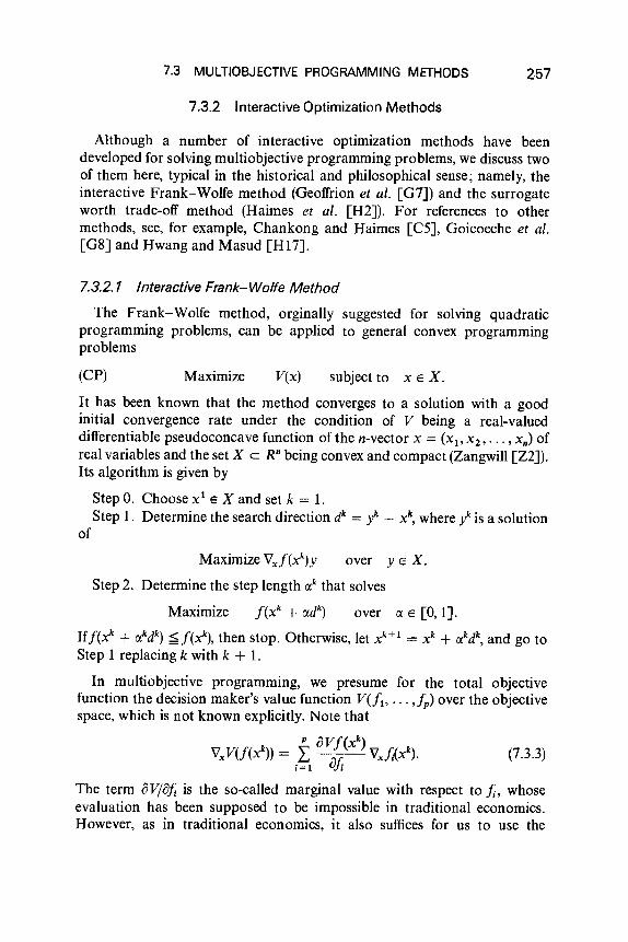
7.3 MULTIOBJECTIVE PROGRAMMING METHODS 257
7.3.2 Interactive Optimization Methods
Although a number of interactive optimization methods have beendeveloped for solving multiobjective programming problems, we discuss twoof them here, typical in the historical and philosophical sense; namely, theinteractive Frank-Wolfe method (Geoffrion et al. [G7]) and the surrogateworth trade-off method (Haimes et al. [H2]). For references to othermethods, see, for example, Chankong and Haimes [C5], Goicoeche et al.[G8] and Hwang and Masud [HI7].
7.3.2.1 Interactive Frank-Wolfe Method
The Frank-Wolfe method, orginally suggested for solving quadraticprogramming problems, can be applied to general convex programmingproblems
(CP) Maximize V(x) subject to x E X.
(7.3.3)
It has been known that the method converges to a solution with a goodinitial convergence rate under the condition of V being a real-valueddifferentiable pseudoconcave function of the n-vector x = (x l' X2' .•. , xn) ofreal variables and the set X c R" being convex and compact (Zangwill [Z2]).Its algorithm is given by
Step O. Choose Xl E X and set k = 1.Step 1. Determine the search direction dk = I - x\ where I is a solution
of
Maximize Vxf(xk)y over y E X.
Step 2. Determine the step length ak that solves
Maximize f(x k + adk) over a E [0, 1].
Iff(~ + akdk) ~f(Xk), then stop. Otherwise, let ~+1 = xk + I'J.kd\ and go toStep 1 replacing k with k + 1.
In multiobjective programming, we presume for the total objectivefunction the decision maker's value function V(fl' ... ,fp) over the objectivespace, which is not known explicitly. Note that
p aVf(xk)VxV(f(x
k)) = i~l aj; VxHxk).
The term aV;aj; is the so-called marginal value with respect to ii, whoseevaluation has been supposed to be impossible in traditional economics.However, as in traditional economics, it also suffices for us to use the

258 7 METHODOLOGY
marginal rate of substitution (MRS) instead of the marginal value forour present purpose. Let A = (It, ... ,Jp ) be indifferent to B =(Jl,""]; + 111;, ... ,]j-l1fj, ... ,Jp) . Namely, in order to keep the indif-ference relation between A and B, the improvement of fj by I1fj is requiredfor compensating for the sacrifice of 1; by 111;. Then the marginal rate ofsubstitution mij of1; for fj at J is defined as the limit of the rate ofsubstitution I1fjj111; as B tending to A. That is,
I. (l1fj)mij= 1m - .B--+A 111;
As is readily seen, there is a relation between the marginal rate of substitutionand the marginal value
mij = (oVjoJ;)j(oVjofj).
Hence, the relation (7.3.3) can be rewritten as
Note here that the term OV(fk)jofs does not have any effect on the solution ofthe maximization problem (CP), so long as s is selected in such a way that theterm becomes negative at each iteration. Therefore, in using the Frank-Wolfe method for our multiobjective problem in an interactive way, thedecision maker is requested to answer his MRS at Step 1 and the mostpreferred point along the search direction at Step 2.
7.3.2.1.1 Discussion. We have the following questions in the inter-active Frank-Wolfe method:
(i) Can we guarantee the differentiability and quasiconcavity ofV(fb ... ,fp) so that the method may converge?
(ii) How is the MRS of the decision maker assessed?(iii) Can the decision maker make the line search easily?
As to question (i), Wehrung [W6] proved that the convergence property ofthe method under some appropriate conditions on the decision maker'spreference rather than the value function V(f) is
(l) complete,(2) transitive,(3) continuous in the sense that both sets
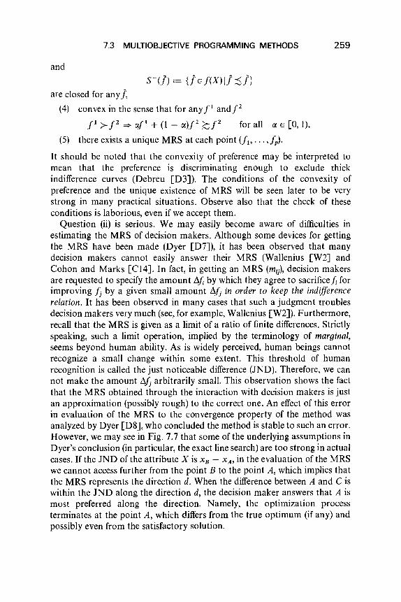
7.3 MULTIOBJECTIVE PROGRAMMING METHODS 259
and
are closed for any],
(4) convex in the sense that for anyr andj?
fl >- P => (Xfl + (l - cx)p ?::J2 for all a E [0, I),
(5) there exists a unique MRS at each point (fh ... ,fp).
It should be noted that the convexity of preference may be interpreted tomean that the preference is discriminating enough to exclude thickindifference curves (Debreu [D3]). The conditions of the convexity ofpreference and the unique existence of MRS will be seen later to be verystrong in many practical situations. Observe also that the check of theseconditions is laborious, even if we accept them.
Question (ii) is serious. We may easily become aware of difficulties inestimating the MRS of decision makers. Although some devices for gettingthe MRS have been made (Dyer [D7]), it has been observed that manydecision makers cannot easily answer their MRS (Wallenius [W2] andCohon and Marks [CI4]. In fact, in getting an MRS (mi), decision makersare requested to specify the amounr af by which they agree to sacrificej, forimproving Jj by a given small amount !J.fj in order to keep the indifferencerelation. It has been observed in many cases that such a judgment troublesdecision makers very much (see, for example, Wallenius [W2]). Furthermore,recall that the MRS is given as a limit of a ratio of finite differences. Strictlyspeaking, such a limit operation, implied by the terminology of marginal,seems beyond human ability. As is widely perceived, human beings cannotrecognize a small change within some extent. This threshold of humanrecognition is called the just noticeable difference (JND). Therefore, we cannot make the amount !1Jj arbitrarily small. This observation shows the factthat the MRS obtained through the interaction with decision makers is justan approximation (possibly rough) to the correct one. An effect of this errorin evaluation of the MRS to the convergence property of the method wasanalyzed by Dyer [D8], who concluded the method is stable to such an error.However, we may see in Fig. 7.7 that some of the underlying assumptions inDyer's conclusion (in particular, the exact line search) are too strong in actualcases. If the JND of the attribute X is XB - XA, in the evaluation of the MRSwe cannot access further from the point B to the point A, which implies thatthe MRS represents the direction d. When the difference between A and Ciswithin the JND along the direction d, the decision maker answers that A ismost preferred along the direction. Namely, the optimization processterminates at the point A, which differs from the true optimum (if any) andpossibly even from the satisfactory solution.

260 7 METHODOLOGY
d
I,I,II I, I,-JND-ooI
optimal
Q5;tion
'------'--....I-----------------xFig. 7.7.
Note here that, in the presence of the JND, indifference curves in a usualsense cannot so much as exist (and hence neither can the MRS), because theJND causes an intransitive indifference. For more details on the JND andintransitive indifference, see Chipman [C9J, Luce [Ll l ], and Tversky [T1S].
Question (iii) is not as severe as question (ii). Recall that we cannot expectthe exact line search even in traditional mathematical programming withexplicitly known objective functions; hence, it suffices for convergence to findan approximate pointJmore preferable to fk. Even so, it is not very easy fordecision makers to answer a more preferable point along the direction,because it requires them to rank vectors, that is, to evaluate multiple criteriasimultaneously. In particular, this situation becomes severe as we come closeto the solution. Furthermore, poor line searches cause poor rates ofconvergence. Wehrung [W7] suggested a method that determines a subset ofa predetermined finite number of equal subintervals of Uk, IJ based on theFibonacci search method, the golden section method, the bisection method,and other methods. On the other hand, Oppenheimer [OlJ suggested theiterative utilization of a proxy function with a known form as a localapproximation of V(f(x)). As a proxy function, he suggested the use of theexponential sum
p
P1(f) = - L aiexp(-w;fJ;=1
or the power sump
P2(f) = - L a.f]".i=1

7.3 MULTIOBJECTIVE PROGRAMMING METHODS 261
The parameters a., w;, and lXi are decided for Pt , for example, by solving theequation
mij = (oP(f)/o/i)(oP(f)/ofj)
Using Oppenheimer's method, the number of assessments of the decisionmaker's preference is expected to decrease. However, in general, theconvergence (and convergence rate) would be sensitive to the form of proxyfunction and the assessed MRS.
7.3.2.2 The Surrogate Worth Trade-Off Method
If the less of each objective functionj, is preferred to the more, it is naturalto consider the decision maker's preference to be monotonous; namely,
Then, according to Theorem 3.1.1, the most preferable solution with respectto the decision maker's preference should belong to the set of efficientsolutions. In the Geoffrion-Dyer-Feinberg method, the obtained solutionmay be proved theoretically to be an efficient solution under some appro-priate conditions such as the convexity of the preference, the criteria j., andthe set X. In practice, however, this cannot necessarily be expected due toseveral kinds of errors including human factors. Haimes et al. [H2] suggesteda method, called the surrogate worth trade-off (SWT) method, in which thesearch is limited on the efficient set without using decision makers' MRSexplicitly. Before stating the method, note the following property of thepreferentially optimal solution.
Assumption 7.3.1
The set of efficient solutions in the objective space defines a smooth surfaceE in RP.
Definition 7.3.1 (Efficiency Trade-Off Ratio)
Let (t 1, ••• , tp-Ill) denote the direction ratio of the outer normal of Eatan efficient point]. Then tj gives information on the trade-off between f p andfj at the point I for keeping the efficiency. Therefore, t j is called the efficiencytrade-off ratio between j, andjj.
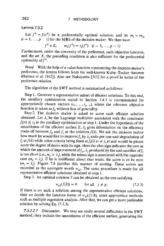
262 7 METHODOLOGY
Lemma 7.3.2
Let fO = f(xO) be a preferentially optimal solution, and let mi = mip(i = 1, ... , p - 1) for the MRS of the decision maker. We then have
fO E E, mi(f°) = tUO) (i = 1, .. . .p - 1)
Furthermore, under the convexity of the preference, each objective function,and the set X, the preceding condition is also sufficient for the preferentialoptimality «i».
Proof With the help of a value function representing the decision maker'spreference, the lemma follows from the well-known Kuhn-Tucker theorem(Haimes et al. [H2]). Also see Nakayama [N3] for a proof in terms of thepreference relation.
The algorithm of the SWT method is summarized as follows:
Step 1. Generate a representative subset of efficient solutions. To this end,the auxiliary optimization stated in Section 3.4.3 is recommended forappropriately chosen vectors (S1>"" Sp-I), where the reference objectivefunction is taken esf; without loss of generality.
Step 2. The decision maker is asked to score each efficient solutionobtained. Let Aj be the Lagrange multiplier associated with the constraintfix) ~ Sj in the auxiliary optimization at step 1. Under the hypothesis of thesmoothness of the efficient surface E, Aj gives information on the efficiencytrade-off between fp and fj at the solution f(x). We ask the decision makerhow much he would like to improvej, by Ajunits per one-unit degradation offj atf(x) while other criteria being fixed at!.(x) (s #- j, p) and would he pleasescore the degree of desire with its sign. Here the plus sign indicates the case inwhich the amount of improvement offp , Ajproduced by the unit sacrifice offjis too short (i.e.,mj > A), while the minus sign is associated with the oppositecase (mj < Aj)' If he is indifferent about that trade, the score is to be zeroim, = AJ Figure 7.8 justifies this manner of scoring. These scores arerecorded as the surrogate worth Wpj' The same procedure is made for allrepresentative efficient solutions obtained at step 1.
Step 3. An optimal solution x can be obtained as the one satisfying
for all j #- p. (7.3 .3)
If there is no such a solution among the representative efficient solutions,then we decide the function forms of Wpj(f) by some appropriate methodssuch as multiple regression analysis. After that, we can get a most preferablesolution by solving Eq. (7.3.3).
7.3.2.2.1 Discussion. We may see easily several difficulties in the SWTmethod; they include the smoothness of the efficient surface, generating the

7.3 MULTIOBJECTIVE PROGRAMMING METHODS 263
fiX}
efficient curve
L..---,-----i------'--------- fj
Wi
+
o I---"t---__~----------- fj
Fig. 7.8. SWT method.
representative set of efficient solutions, scoring the surrogate worth, andmultiple regression and solving a system of nonlinear equations Wpj(x) = O.We shall discuss these points below.
The smoothness of the efficient surface is guaranteed only for limited cases,for example, in which each objective function is smooth and strictly convex.If the efficient surface is not smooth, we could have a condition for the prefer-ential optimality of fO
-(mb"" mp-b 1) E (T(f(X),j°))O

264 7 METHODOLOGY
(see, for example, Nakayama [N3]). In this case, the Lagrange multiplier(Al' ... , Ap-lo 1) obtained by the auxiliary optimization at step 1 is merely avector of ((T(f(X),f°W, and hence mj = Aj U= 1, ... , p - 1) cannot beexpected, in general.
We need to solve an auxiliary nonlinear optimization problem in order toget an efficient solution. In many practical problems, this step requires muchcomputational effort, and hence the least number of representative efficientsolutions is more desirable. However, if the number is too few, then the mostpreferable solution might not be in the given representative efficient set. Thecase, therefore, charges us with the extra effort of multiple regression andsolving the nonlinear equations Wpj = O.
In the original version of the SWT method, the surrogate worth is neededonly to score an ordinal measure. However, since such an ordinal score doesnot make sense for comparison of the differences among them, thesubsequent multiple regression and the nonlinear equation wpj(f(x)) = 0 arevery difficult to solve. In Chankong and Haimes [C6], the surrogate worth issupposed to be scored by a cardinal measure. However, the consistency ofthe surrogate worth as a cardinal measure becomes a new problem.
In cases with only a few objective functions, a solution satisfyingwpi!(x)) = 0 U= 1, ... , p - 1)may be relatively easily obtained in the givenrepresentative efficientset. In these lucky cases, we do not need to invoke themultiple regression analysis to get the function form of Wpj(f) and solve thesystem of nonlinear equations wpif) = O. In general, however (particularlyin cases with a large number of objective functions) such a lucky case ishopeless, and, therefore, the stated extra efforts are needed. The difficulty forthese operations has been seen in the preceding discussion for the ordinalsurogate worth.
In order to overcome some of these difficulties, several modifications havebeen developed. Note that in the SWT method since the search is restrictedon the efficient surface, the independent variable is the p - l-dimensionalvector (flo ... ,!P-l)' Let the efficient surface be represented by the equationE(ft> '" ,fp) = O. If we have f p = w(flo ... ,fp-l) by solving the equation,then for the value function restricted on the efficient surface E,
V(fj, ... ,fp-l) .= V(ft>·· .,fp-l' w(ft> .. ·,fp-d)
Vj = Vj + "VpWj U= 1, .. . ,p -1), (7.3.4)
where "f0 = 8V/8Jj, Vj = 8V/iJJj, and Wj = 8w/8Jj. On the other hand, on theefficient surface E,
Ej+EpWj=O (j=I, ... ,p-I)
where Ej = 8E/iJJj. Therefore, making use of the fact that
m, = Vj/v" and tj = Ej/Ep,
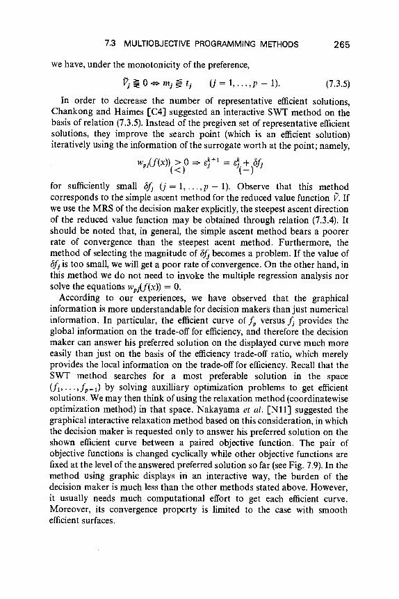
7.3 MULTIOBJECTIVE PROGRAMMING METHODS 265
we have, under the monotonicity of the preference,
u= 1, .. . ,p -1). (7.3.5)
In order to decrease the number of representative efficient solutions,Chankong and Haimes [C4] suggested an interactive SWT method on thebasis of relation (7.3.5). Instead of the pregiven set of representative efficientsolutions, they improve the search point (which is an efficient solution)iteratively using the information of the surrogate worth at the point; namely,
Wpj(l(x» > 0 => eJ+l = eJ + fJJj«) (-)
for sufficiently small fJJj U = 1, ... , p - 1). Observe that this methodcorresponds to the simple ascent method for the reduced value function V. Ifwe use the MRS of the decision maker explicitly, the steepest ascent directionof the reduced value function may be obtained through relation (7.3.4). Itshould be noted that, in general, the simple ascent method bears a poorerrate of convergence than the steepest acent method. Furthermore, themethod of selecting the magnitude of fJJj becomes a problem. If the value offJJj is too small, we will get a poor rate of convergence. On the other hand, inthis method we do not need to invoke the multiple regression analysis norsolve the equations wpif(x» = O.
According to our experiences, we have observed that the graphicalinformation is more understandable for decision makers than just numericalinformation. In particular, the efficient curve of fp versus Jj provides theglobal information on the trade-off for efficiency, and therefore the decisionmaker can answer his preferred solution on the displayed curve much moreeasily than just on the basis of the efficiency trade-off ratio, which merelyprovides the local information on the trade-off for efficiency. Recall that theSWT method searches for a most preferable solution in the space(It> ... ,fp-l) by solving auxilliary optimization problems to get efficientsolutions. We may then think of using the relaxation method (coordinatewiseoptimization method) in that space. Nakayama et al. [Nll] suggested thegraphical interactive relaxation method based on this consideration, in whichthe decision maker is requested only to answer his preferred solution on theshown efficient curve between a paired objective function. The pair ofobjective functions is changed cyclically while other objective functions arefixed at the level of the answered preferred solution so far (see Fig. 7.9). In themethod using graphic displays in an interactive way, the burden of thedecision maker is much less than the other methods stated above. However,it usually needs much computational effort to get each efficient curve.Moreover, its convergence property is limited to the case with smoothefficient surfaces.
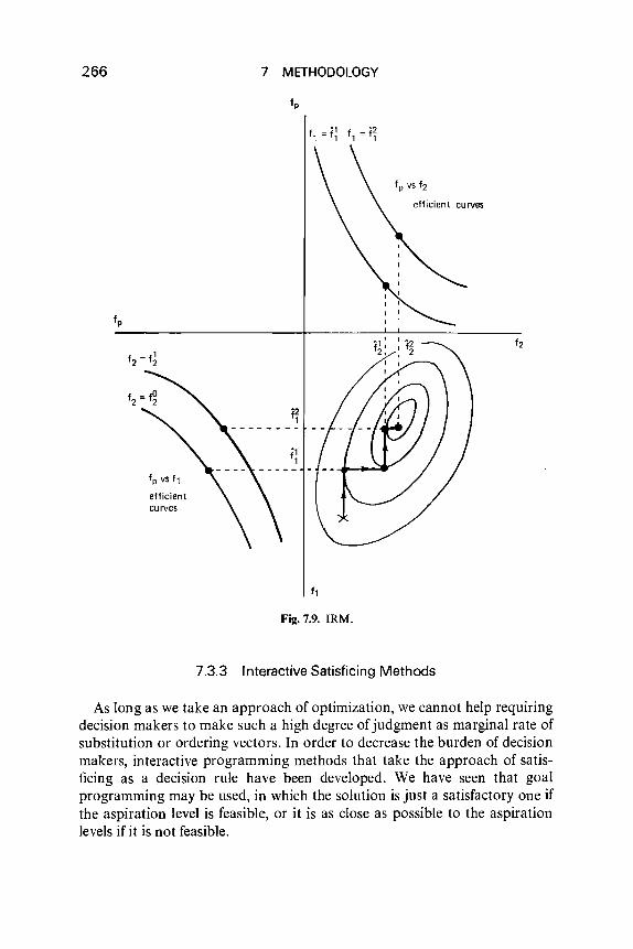
266
fp vs fl
efficientcurves
7 METHODOLOGY
fp vs f2
efficient curves
Fi~. 7.9. IRM.
7.3.3 Interactive Satisficing Methods
As long as we take an approach of optimization, we cannot help requiringdecision makers to make such a high degree of judgment as marginal rate ofsubstitution or ordering vectors. In order to decrease the burden of decisionmakers, interactive programming methods that take the approach of satis-ficing as a decision rule have been developed. We have seen that goalprogramming may be used, in which the solution is just a satisfactory one ifthe aspiration level is feasible, or it is as close as possible to the aspirationlevels if it is not feasible.

7.3 MULTIOBJECTIVE PROGRAMMING METHODS 267
Note here that satisficing was originally suggested due to the observationof the limit of human cognitive ability and available information throughdecision making (Simon [S9J). In our problem formulation, however, we aresupposed to be able to evaluate the values of criteria functions by somemeans, although we also observe the limit of human cognitive ability. Forthese problems, mere satisficing is not necesarily satisfactory to the decisionmaker as a decision rule.
For example, let us consider a case in which a decision maker ordered twodesigners to design some industrial product. Almost at the same time andalmost at the same expense, these two designers completed their designs,which were both satisfactory to the decision maker. However, one of thedesigns is superior to the other in terms of all criteria. In this case, thereseems no doubt that the decision maker should adopt the superior one. Thisexample allows us to use a solution x which is satisfactory and in additiongurantees that there is no other feasible solution that is superior to xin termsof all criteria.
Definition 7.3.2 (Satisfactory Pareto Solution)
A solution that is satisfactory and (weakly) Pareto efficient is called asatisfactory (resp. weak) Pareto solution. In other words, when f is anaspiration level of the decision maker, an alternative x is said to be asatisfactory Pareto solution if
and
f(x) i: f(x) for all x E X
f(x) ~ f.A satisfactory weak Pareto solution can be defined analogously by replacingi with v; in the first inequality.
In general, satisfactory (weak) Pareto solutions constitute a subset of X.However, we can narrow down the set of satisfactory Pareto solutions andobtain a solution close to the preferentially optimal one by tightening theaspiration level, if necessary. On the other hand, even if there does not existany satisfactory Pareto solution for the initial aspiration level, we can attainone by relaxing the aspiration level. Originally, the aspiration level is fuzzyand flexible. It seems that decision makers change their aspiration levelsaccording to situations.
From this point of view, the interactive satisficing methods provide a toolthat supports decision makers in finding an appropriate satisfactory (weak)Pareto solution by some adjustment of the aspiration level. Usually theaspiration level is changed in such a way that
I:" = To p(fk),
268 7 METHODOLOGY
wherer represents the aspiration level at the kth iteration. The operator Pselects the Pareto solution nearest in some sense to the given aspiration levelr.The operator T is the trade-off operator, which changes the kth aspirationIevelj" if the decision maker does not compromise with the shown solutionP(Jk). Of course, since P(]k) is a Pareto solution, there exists no feasiblesolution that makes all criteria better than p(Jk), and the decision makermust trade-off among criteria if he wants to improve some of criteria. Basedon this trade-off, a new aspiration level is decided as To P(Jk). The process iscontinued until the decision maker obtains an agreeable solution.
7.3.3.1 STEM
STEM (Step Method) by Benayoun et al. [B6] was originally developedfor solving linear multiobjective programming problem, and its extension togeneral nonlinear cases is straightforward (Shimizu [S8]). The followingdiscussion will be made for nonlinear multiobjective problems.
LetJ* be an ideal point, and let us try to find a solution as close as possibleto this ideal point. Although several distance function may be available as ingoal programming, Zoo-norm is usually recommended:
Min Max Jld};(x) - JilxeX l~i~p
subject to
f(x) - Jt ~ t1f, (i = 1, ... , p),
where t1f is an admissible deviation from the ideal levelj',".Equivalently,
Min ~x,~
Jli(f(x) - Ji*) ~ ~,
f(x) - Ji* ~ !1f
X E X.
subject to
(i=l, ,p)
(i = 1, , p)
Note here that the aspiration level is given by]; = J;* + t1f. The solutionto these problems is clearly a satisfactory weak Pareto solution if theaspiration level is feasible; namely,] E J(X), However, taking into accountthe total balance among the levels of objective functions at the obtainedsolution, decision makers are sometimes dissatisfied with some of them.More importantly, the aspiration level might happen to be infeasible in somecases. Under such a circumstance, some of aspiration levelsshould be relaxedin order to get a satisfactory solution. In other words, the decision maker isnow faced with a trade-off problem.

7.3 MULTIOBJECTIVE PROGRAMMING METHODS 269
On the basis of the above consideration, STEM and its modificationsprovide a tool for getting a reasonable solution by changing the aspirationlevel in an interactive way.
Step O. Set k = 1, and determine the ideal pointf* and the weight Ili bysome appropriate way (see Remark 7.3.4 later). Find a solution xk to thefollowing problem:
Minex,~
subject to Ili(/;(X) - f;*) ~ e, (i = 1, ... , p) X E X.
Step 1. Seeing f(xk) obtained above, the decision maker classifies the
objective functions into two classes: the ones with satisfactory levels (its indexset is denoted by S) and the ones with unsatisfactory levels (its index set isdenoted by U). If there is no unsatisfactory /;, then the iteration terminates.Otherwise the decision maker relaxes the level of the satisfactory objectivefunctions, whose amount is set 11/;.
Step 2. Solve
Min~x.~
subject to
Ili(/;(X) - fi*) ~ e, i E U,
/;(x) - fi* ~ 11/;, i E S,
X E X.
Set the solution to be xk +1 and return to step 1.
Remark 7.3.4
In using the la-type distance function, it is very important to make acommon scale for the objective functions. For example, if the positive andnegative values of the objective functions are mixed, or if their numericalorders are extremely different from each other, then in the Min-Maxproblem some of objective functions are sensitive and others not. Note thatthe origin is set up by the ideal pointf*, and the weight Ili corresponds to thescale factor.
In STEM the ideal pointf* is set by
/;* = Min /;(x) := N(xt),XEX
and the weight Ili is given by normalizing
tr-> J.* ( ~)-1w; = ' /; '. Vj~l c~ ,

270 7 METHODOLOGY
f, f2 fp
f, f~(X1) f2(Xi) ....... fp(Xi)
f2 f, (X2) f;(X2) ....... fp (X2)
f*(x*)p p
Fig. 7.10. Payoff matrix.
where cij is the coefficient of the ith objective function};(x) = I CijXj,fimax isthe maximum component of the ith row vector in the so-called payoff matrixgiven by Fig. 7.10 and}; = fimax iffimax > 0, otherwise}; = Ifn
7.3.3.1.1 Discussion. Intuitively speaking, the stated method relaxesthe objective functions that attain their aspiration levels at an early stage anddistributes the benefit caused by their sacrifice to other objective functionsequally; the process is continued until all objective functions becomesatisfactory. However, it is not clarified just how much sacrifice of someobjective functions gives how much improvement to other objective func-tions. As a result, it is up to the decision maker's guess with the help of thepayoff matrix. Additionally, in many practical cases, the decision makerdesires to improve some of the objective functions much more strongly thanhe may agree to sacrifice others. Therefore, it seems more natural to ask thedecision makers how much they want to improve unsatisfactory objectives aswell as how much they agree to sacrifice satisfactory ones. From this point ofview, Wierzbicki [W13, W14] and Lewandowski and Grauer [L5] suggesteda method called the reference point method or dynamic interactive decisionanalysis support systems (DIDASS) (see also Grauer et al. [G9]).Independently from their works, Nakayama [N4, N8] also developed asimilar method called the satisficing trade-off method, which will bediscussed in more detail later.

7.3 MULTIOBJECTIVE PROGRAMMING METHODS 271
efficient curve
Min-Max solutioncorresponding tothe aspirationlevel fw
band ofaspiration level
Min-Max solutioncorresponding tothe aspirationlevel tb
f*
Fig, 7.11. Satisficing trade-off method.
7.3.3.2 Satisficing Trade-Off Method
First, we note several important properties for the Min-Max problem(Fig. 7.11)
(P00) Min Max /lJj;(x) - fnXEX l~i~p
Lemma 7.3.3
For fi* < Min{/;{x): x E X}, each Pareto solution can be obtained bysolving the Min-Max problem (P00) with an appropriate positive weight /li(i = 1, ... ,p).
Proof Immediate from Theorem 3.4.9.
Lemma 7.3.4
Suppose that for any x E X
fi* </;{x), (i = 1, .. . ,p). (7.3.6)
If we set for a given aspiration level J with J > f*
/li = 1/(]; - fn (i = 1, ... , p), (7.3.7)

272 7 METHODOLOGY
then the solution x to the Min-Max problem (PC<) is a satisfactory weakPareto solution in case of] being feasible, while it is assured to be a weakPareto solution even in case of] being infeasible.
Proof It is well known that the solution to the Min-Max problem (PC<) isa weak Pareto solution. Hence, we shall show that if the aspiration level] isfeasible, then the solution x to the Min-Max problem becomes a satisfactorysolution; namely.j'(x) ~ f.
Let
and define the level set at] by
L := {y = (Yb" .,Yp)lp(y) ~ pU)}.
Furthermore, setting
S := {y = (YI,' .. ,Yp)IYi ~];, i = 1, .. . ,p},
we have
L c S. (7.3.8)
In fact, the way of setting the weight Jii yields Jid]; - tt I = 1 (i = 1, ... ,p),and hence for any Y ELand i = 1, ... , p,
JiilYi - fi*1 ~ Jil]; - Inwhich yields Yi ~]; (i = 1, ... , p).
Now note that ifJis feasible, then there exists an X E X such that/;(x) ~];
for all i = 1, ... , p. Then
Jid/;(~) - fil = Jil/;(~) - fn
s Jill; - m.
thereby
{f(x)lx E X} II L i: 0. (7.3.9)
Relations (7.3.8) and (7.3.9) imply that the solution to Min x e x p(f(x) belongsto the set S.
Lemma 7.3.5
Let (x, ~) be a solution to
(P;") Min ~ subject to Jii(/;(X) - H) ~ ~,x.~
(i = 1, ... , p), x E X,

7.3 MULTIOBJECTIVE PROGRAMMING METHODS 273
which is equivalent to the Min-Max problem (P"',), and let ~ = (~1' ... , ~p) bethe optimal Lagrange multipliers. If x is interior to the set X and eachfi hasappropriate smoothness, then we have
p -
I A; = 1,;=1
~; ~ 0, (i = 1, . .. ,p) (7.3.10)
p -I A;f1.i Vfi(x) = O.;=1
(7.3.11)
Moreover, if the problem (P:.,) is convex, namely, if eachfi is convex and theset X is convex, then for any x E X
p -
I Aif1.i(fi(x) - fi(x» ~ o.;=1
(7.3.12)
Proof Relations (7.3.10) and (7.3.11) immediately follow from the well-known Kuhn-Tucker theorem for the Lagrangean
p
L(x, ~ : A) = ~ + I A;(f1.;(j;(x) - ft» - ~).i=1
In addition, the well-known theory of convex programming provides that forthe solution (x, ~) and ~ and for all x E X and ~
L(x, ~:~) ~ us, ~: ~),
from which relation (7.3.12) follows by virtue of If=I~; = 1.
The algorithm of the satisficing trade-off method is summarized as follows:
Step 1 (setting the ideal point). The ideal point f* = (ft, .. .,ft) is set,wherej;* is small enough [for example,j;* = Min{j;(x) Ix EX} - 8 (8) 0)].This value is fixed throughout the following process.
Step 2 (setting the aspiration level), The aspiration levelj'] of each objectivefunction fi at the kth iteration is asked of the decision maker. Here n shouldbe set in such a way that n > it (i = 1,.", p). Set k = 1.
Step 3 (weighting and finding a Pareto solution by the Min-Maxmethod). Set
f1.f = 1/(];k - fnand solve the Min-Max problem
(P~) Min Max f1.flfi(x) - HIXEX l~i~p
(7.3.13)
or equivalently
(P~) Min ~ subject to f1.f(fi(x) - fi*) ~~, (i = 1, ... , p), x E X.X,~
Let xk be a solution to these problems.
274 7 METHODOLOGY
Step 4 (trade-off). Based on the value off(xk), the decision maker classifies
the criteria into three groups, namely, the class of criteria that he wants toimprove more, the class of criteria that he may agree to relax, and the class ofcriteria that he accepts as they are. The index set of each class is representedby n, It It respectively. If n= 0, then stop the procedure. Otherwise, thedecision maker is asked his new acceptable level of criteriaR for the class ofnand I~. For i E I~, setJt = };(xk
) .
Step 5 (feasibility check). Let ...1.; (i = 1, ... , p) be the optimal Lagrangemultipliers to the problem (P~). If for a small nonnegative 8
p
I ...1.;J1~(R - };(xk) ) ~ -G,
;=1
(7.3.14)
set the new aspiration level It +1 asR and return to the step 3; otherwise.jj'might be infeasible in the sense of linear approximation as will be explainedlater. By taking the degree of difficulty for solving the Min-Max probleminto account, we choose either to trade offagain or to return to the step 3 bysetting Jt+l = R. In the case of trading off again, the acceptable level ofcriteria for nand/or I~ should be reset lower than before, and then return tothe beginning of the step 5.
The outstanding features of the satisficing trade-off method include. thefollowing:
(1) We do not need to pay much attention to setting the ideal pointf*. Itsuffices to setf* sufficiently small enough to cover all or almost of all Paretosolutions as candidates for a decision solution in the following process.In case in which Min{};(x) Ix E X} is finite, for example, set ir =Min{/;(x) Ix E X} - 8 (8 > 0). Otherwise, setfi* to be sufficiently small.
(2) The weights J1; (i = 1, ... ,p) are automatically set by the ideal pointf*and the aspiration level f. For the weight in Eq. (7.3.13), the value ofJ1;(f;* - };(x)) can be considered to represent the normalized degree ofnonattainability of /;(x) to the ideal point tr. This enables us to ignore theneed to pay extra attention to the difference among the dimension and thenumerical order of criteria.
(3) By solving the Min-Max problem under the preceding conditions wecan get a satisfactory weak Pareto solution in the case in which the aspirationlevelJ is feasible, and a weak Pareto solution even in the case in whichJ isunfeasible. Interpreting this intuitively, in case in which J is feasible theobtained satisfactory weak Pareto solution is the one that improves equallyin some sense each criterion as much as possible, and in case in which J isinfeasible we get a weak Pareto solution nearest to the ideal point that sharesan equal amount of normalized sacrifice for each criterion. This practical

7.3 MULTIOBJECTIVE PROGRAMMING METHODS 275
meaning encourages the decision maker to accept easily the obtainedsolution.
(4) At the stage of trade-off, the new aspiration level is set in such a waythat
for any i E n,for any i E It
In this event, if Jk+l is feasible, then in view of Lemma 7.3.4 we have asatisfactory weak Pareto solution by solving the Min-Max problem. Insetting the new aspiration level, therefore, it is desirable to pay attention sothat] becomes feasible.
(5) In order that the new aspiration level]k+l may be feasible, the criteriah (i E I~) should be relaxed enough to compensate for the improvement ofh(xk
) (i E m. To make this trade-off successful without solving a new Min-Max problem, we had better make use of sensitivity analysis based onLemma 7.3.5. Since we already know xk is a Pareto solution, the feasibility ofxk+ 1 can be checked by relation (7.3.14). Here /; is introduced to makerelation (7.3.14)available for nonconvex cases in which relation (7.3.12)doesnot necessarily hold. Moreover, observe in view of Eq. (7.3.11) that
(i = 1, ... , p) (7.3.15)
represents the efficient trade-off, which reflects the mutual effect of change ofeach criterion restricted to the Pareto surface. Based on this information ofefficienttrade-off, the decision maker can easilyjudge how much the criterionI, for i E I~ should be improved and how much the criteria j, for i E I~ shouldbe relaxed. In particular, since a little relaxation ofjj withj such that Aj = 0cannot compensate the improvement of fi (i E munder the condition thatJk+ 1 should be on the Pareto surface, we must relax at least one jj for j suchthat Aj =1= 0 or give a sufficientlylarge relax for jj such that Aj = O.
Remark 7.3.4
The stated feasibility check is just for the purpose of decreasing the numberof Min-Max problems that must be solved and is not necessarily performedstrictly. In some cases, several trials for trade-off cannot succeed in holdingrelation (7.3.14)and the decision maker would tend to be tired of trading offagain and again. In this circumstance, we had better go to solving Min-Maxproblem immediately even if relation (7.3.14) does not hold. However, incases that require a lot of effort to solve Min-Max problems, a few retrials oftrade-off could not be helped.
276
Remark 7.3.5
7 METHODOLOGY
In some cases, decision makers want to know the global feature of thefeasible set in trading-off. To this end, it is convenient to show the so-calledpayoff matrix by minimizing each objective function independently, whichwas introduced in STEM. Of course, since the payoff matrix does not changeduring the interactive process, systems analysists had better prepare it inadvance of the decision process.
Remark 7.3.6
It may be possible to change the ideal pointf* while the aspiration level]is fixed during the decision process. This is considered to be a dual approachof the satisficing trade-off method. However, if the initial aspiration levelhappens to be a Pareto solution, then we cannot get other Pareto solution bysolving the Min-Max problem as long as the aspiration level is fixed. Hence,when the decision maker wants another solution, he ,must change theaspiration level. Taking such a case into account, the way of changing theaspiration level seems better.
7.3.3.2.1 Discussion. As we have seen earlier, the solution obtained bythe satisficing trade-off method as well as STEM is not necessarily a Paretosolution but is guaranteed only to be a weak Pareto solution. For weakPareto solutions, there may exist another solution that improves somecriteria while other criteria are left unchanged, and hence weak Paretosolutions seem to be inadequate as a decision making solution. We can get aPareto solution from a weak Pareto solution as follows:
(AP) Maximize
hex) + e, = hex),
X EX,
subject to
(i = 1, , p)
(i = 1, , p)
where ~ is a (weak) Pareto solution. Ifall e, for the solution to (AP) are zero,then x itself is a Pareto solution. If there are some [;i oj; 0, then the solution xto problem (AP) is a Pareto solution.
However, in some practical problems it is very expensive to perform suchan auxilliary optimization. In order to avoid such an additional scalaroptimization problem, some researchers suggested the use of some kinds of

7.3 MULTIOBJECTIVE PROGRAMMING METHODS 277
augmented norms (Oinkelbach and Isermann [06J; Steuer and Choo [S14J).One typical example is given by
(7.3.16)
Recall that, in general, in interactive satisficing methods the aspirationlevel is changed by r+ 1 = To p(Jk), where P is an operator that finds thePareto solution nearest in some sense to the aspiration levelr. This can bedone by using some scalarization function. The sense of nearest stronglydepends on what kind of the scalarization function we use. We impose thefollowing requirements on the scalarization functions:
1. They can cover all Pareto solutions.2. Solutions to the auxilliary scalar optimization should be Pareto
solutions.3. Solutions to the auxiliary scalar optimization should be satisfactory, if
the aspiration level is feasible.
Since our decision-making solution is a satisfactory Pareto solution, thescalarization function should hold the property that its maximization orminimization with appropriately chosen parameters can produce any Paretosolution in order to be applicable for any cases no matter what the problemmay be and no matter what the preference of the decision maker may be.Furthermore, the solution to the auxilliary scalar optimization for thescalarization function should be nothing but a Pareto solution, because ouraim is to find a satisfactory Pareto solution. Finally, if the aspiration level isfeasible, then there exists a satisfactory Pareto solution. Therefore, it wouldnot make sense to show the decision maker a nonsatisfactory solution whenthe aspiration level is feasible. These observations make the preceding threerequirements reasonable.
Unfortunately, it should be noted, however, that there is no scalaraizationfunction satisfying all these requirements. It is well known that lrnormcannot necessarily yield any Pareto solution if the problem is nonconvex.Even if we use an la-norm (1 < or: < 00), we cannot always get all Paretosolutions depending on the degree of nonconvexity of the problem. In Fig.7.12, we can see that the only norm (scalarization function) that can yieldsany Pareto solution in any problem is the weighted Tchebyshev norm.However, the weighted Tchebyshev norm violates requirement 2. Namely,the weighted Tchebyshev norm produces not only Pareto solutions but alsoweak Pareto solutions. For any 0 < (X < 00, the solution obtained byminimizing Sa is guaranteed to be a Pareto solution. However, it can beeasily seen that the augmented norm Sa violates requirements 1 and 3 (Fig.
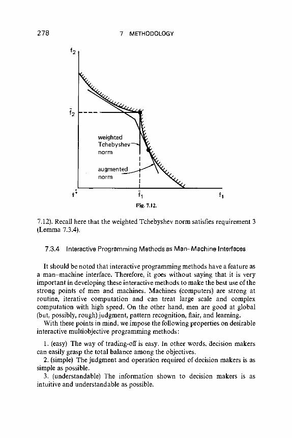
278
.f*
7 METHODOLOGY
weightedTchebyshevnorm
f1
Fig. 7.12.
7.12). Recall here that the weighted Tchebyshev norm satisfies requirement 3(Lemma 7.3.4).
7.3.4 Interactive Programming Methods as Man-Machine Interfaces
It should be noted that interactive programming methods have a feature asa man-machine interface. Therefore, it goes without saying that it is veryimportant in developing these interactive methods to make the best use of thestrong points of men and machines. Machines (computers) are strong atroutine, iterative computation and can treat large scale and complexcomputation with high speed. On the other hand, men are good at global(but, possibly, rough) judgment, pattern recognition, flair, and learning.
With these points in mind, we impose the following properties on desirableinteractive multiobjective programming methods:
1. (easy) The way of trading-off is easy. In other words, decision makerscan easily grasp the total balance among the objectives.
2. (simple) The judgment and operation required of decision makers is assimple as possible.
3. (understandable) The information shown to decision makers is asintuitive and understandable as possible.

7.3 MULTIOBJECTIVE PROGRAMMING METHODS 279
4. (quick response) The treatment by computers is as quick as possible.5. (rapid convergence) The convergence to the final solution is rapid.6. (explanatory) Decision makers can easily accept the obtained solution.
In other words, they can understand why it is so and what it came from.7. (learning effect) Decision makers can learn through the interaction
process.
Interactive programming methods seem promising, in particular for designproblems. However, in applying optimization techniques, we often encountersome difficulties. For example, in structural design problems such as bridges,function forms of some of criteria cannot be obtained explicitly, and theirvalues are usually obtained by complex structural analysis. Similarly, valuesof criteria in the design of camera lenses are obtained by simulation of raytrace; moreover, the number of criteria is sometimes over 100.
From such a practical viewpoint, many existing interactive optimizationmethods require too many auxiliary optimizations during the wholeinteraction process. Moreover, some of them require too high a degree ofjudgment of decision makers such as the marginal rate of substitution, whichseems to be beyond men's ability.
For the purpose of getting a solution, interactive satisficing methods seemadvantageous, because they are usually simple and easy to carry out.However, the fact that we can obtain a solution with less information ondecision makers' preference is in some cases a demerit as well as a merit. For,in many decision problems, there are multiple persons concerned with thoseproblems, and, hence, it is important to get better mutual understanding andcommunication. To this end, methods providing the preference informationof these people seem rather advantageous. This point is outstanding inparticular for problems of public sectors. Since the real world is complex, it isnot so easy to conclude which method is the best. Many practicalapplications could encourage us to sophisticate methodology in future.

This page intentionally left blank
REFERENCES
AI. Allais, M., and Hagen, O. (eds.), "Expected Utility Hypotheses and the Allais Paradox,"Reidel, Dordrecht, Holland, 1979.
A2. Arrow, K. J., "Social Choice and Individual Values," Wiley, New York, 1957.
A3. Arrow, K. J., 'Essays in the Theory of Risk-Bearing," Markham, Chicago, 1971.
A4. Arrow, K. J., Barankin, E. W., and Blackwell, D., Admissible points of convex sets, in"Contributions to the Theory of Games," H. W. Kuhn and A. W. Tucker, (eds.), Vo!. 2,Princeton Univ. Press, Princeton, New Jersey, 1953.
A5. Arrow, K. J.. Hurwicz, L.. and Uzawa, H., "Studies in Linear and Non-LinearProgramming," Stanford Univ. Press, Stanford, California, 1958.
A6. Atkinson, A. B., On the measurement of inequality, J. Econom. Theory 2, 244-263(1970).
A7. Aubin, J. P., "Mathematical Methods of Game and Economic Theory," North-HollandPub!., Amsterdam, 1979.
BI. Barbu, V., and Precupanu, T., "Convexity and Optimization in Banach Spaces," Sijthoffand Noordhoff, Alphen aan de Rijn, 1978.
B2. Baumol, W. H., The cardinal utility which is ordinal, Econom. J. 68, 665-672 (1958).
B3. Bazaraa, M. S., and Shetty, C. M., "Foundations of Optimization," Springer-Verlag,Berlin and New York, 1976.
B4. Bell, D. E., Multiattribute utility functions: decompositions using interpolation,Management Sci. 25, 744-753 (1979).
B5. Bell, D. E., Keeney, R. L., and Raiffa, H. (eds.), "Conflicting Objectives in Decisions,"Wiley, New York, 1976.
B6. Benayoun, R., de Mongolfier, J., Tergny, J., and Larichev, 0., Linear programming withmultiple objective functions: STEP Method (STEM), Math. Programming 1, 366-375(1971).
B7. Benson, H. P., An improved definition of proper efficiency for vector minimization withrespect to cones, J. Math. Anal. Appl. 71, 232-241 (1979).
B8. Benson, H. P., On a domination property for vector maximization with respect to cones,J. Optim. Theory Appl. 39,125-132 (1983).Errata Corrige, J. Optim. Theory 43, 477-479(1984).
281
282 REFERENCES
B9. Benson, H. P., Efficiency and proper efficiency in vector maximization with respect tocones, J. Math. Anal. Appl. 93, 273-289 (1983).
BIO. Benson, H. P., and Morin, T. L., The vector maximization problem: proper efficiencyand stability, SIAM J. Appl. Math. 32, 64-72 (1977).
BII. Berge, C., "Topological Spaces," MacMillan, New York, 1963.
B12. Berge, C., "Graphs and Hypergraphs," North-Holland Pub1., Amsterdam, 1973.
B13. Bitran, G. R., Duality for nonlinear multiple-criteria optimization problems, J.Optim. Theory Appl. 35, 367-401 (1981).
B14. Bitran, G. R., and Magnanti, T. L., The structure of admissible points with respect tocone dominence, J. Optim. Theory Appl. 29, 573-614 (1979).
B15. Bodily, S., Stability, equality, balance and multivariate risk, in "Organizations: MultipleAgents with Multiple Criteria," J. N. Morse, (ed.), Springer-Verlag, Berlin and NewYork,1980.
B16. Borwein, J. M., Proper efficient points for maximizations with respect to cones, SIAM J.ControlOptim. 15, 57-63 (1977).
B17. Borwein, J. M., The geometry of Pareto efficiency over cones, Math. Operationsforsch.und Statist. Ser. Optimization 11, 235-248 (1980).
B18. Borwein, J. M., On the existence of Pareto efficient points, Math. Oper. Res. 8, 64-73(1983).
B19. Borwein, J. M., and Nieuwenhuis, J. W., Two kinds ofnorrnality in vector optimization,Math. Programming 28,185-191 (1984).
B20. Bowman, V. J., Jr., On the relationship of the Tchebycheffnorm and efficient frontiers ofmultiple-criteria objectives, in "Multiple Criteria Decision Making," H. Thriez and S.Zionts, (eds.), Springer-Verlag, Berlin and New York, 1976.
B21. Brumelle, S., Duality for multiple objective convex programs, Math. Oper. Res. 6,159-172 (1981).
CI. Cesari, L., and Suryanarayana, M. B., Existence theorems for Pareto optimization inBanach spaces, Bull. Amer. Math. Soc. 82,306-308 (1976).
C2. Cesari, L., and Suryanayarana, M. B., An existence theorem for Pareto problems,Nonlinear Anal. 2, 225-233 (1978).
C3. Cesari, L., and Suryanayarana, M. B., Existence theorems for Pareto optimization:multivalued and Banach space valued functionals, Trans. Amer. Math. Soc. 244, 37-65(1978).
C4. Chankong, V., and Haimes, Y. Y., "The Interactive Surrogate Worth Trade-Off (ISWT)for Multiobjective Decision-Making," Springer-Verlag, Berlin and New York, 1978.
C5. Chankong, V., and Haimes, Y. Y., On the characterization of noninferior solutions ofthe vector optimization problem, Automatica-J. IFAC 18,697-707 (1982).
C6. Chankong, V., and Haimes, Y. Y., "Multiobjective Decision Making: Theory andMethodology," North-Holland Pub1., Amsterdam, 1"983.
C7. Charnes, A., and Cooper, W., "Management Models and Industrial Applications ofLinear Programming, Vo1. I," Wiley, New York, 1961.
C8. Charnes, A., and Cooper, W. W., Goal programming and multiple objective optimi-zation, J. Oper. Res. Soc. 1, 39-54 (1977).
C9. Chipman, J. S., Consumption theory without transitive indifference, in "Preferences,Utility, and Demand," J. S. Chipman, L. Hurwicz, M. J. Richter, and H. F.Sonnenschein, (eds.), Harcourt Brace Jovanovich, New York, 1971.
REFERENCES 283
CIO. Choo, E. D., and Atkins, D. R., Proper efficiency in nonconvex multicriteria pro-gramming, Math. Oper. Res. 8, 467-470 (1983).
Cll. Clarke, F. H., "Optimization and Nonsmooth Analysis," Wiley, New York, 1983.
C12. Cochrane, J. L., and Zeleny, M., (eds.), "Multiple Criteria Decision Making," Univ, ofSouth Carolina Press, Columbia, South Carolina, 1973.
C13. Cohon, J. L., "Multiobjective Programming and Planning," Academic Press, New York,1978.
C14. Cohon, J. L., and Marks, D. H., A review and evaluation of multi objective programmingtechniques, Water Resources Res. 11,208-220 (1975).
C15. Corley, H. W., An existence result for maximizations with respect to cones, J. Optim.Theory Appl. 31, 277-281 (1980).
C16. Corley, H. W., Duality for maximizations with respect to cones, J. Math. Analy. Appl.84,560-568 (1981).
C17. Craven, B. D., Strong vector minimization and duality, z. Angew. Math. Mech. 60, 1-5(1980).
Dl. Da Cunha, N. 0., and Polak, E., Constrained minimization under vector-valued criteriain finite-dimensional spaces, J. Math. Anal. Appl. 19, 103-124 (1967).
D2. Dantzig, G. B., Folkman, J., and Shapiro, N., On the continuity of minimum set ofcontinuous functions, J. Math. Anal. Appl. 17, 519-548 (1967).
D3. Debreu, G., "Theory of Value," Wiley, New York, 1959.
D4. Delahare, J. P., and Denel, J., The continuities of the point-to-set maps, definitions andequivalences, Math. Programming Study. 10,8-12 (1979).
D5. Diamond, P. A., Cardinal welfare, individualistic ethics, and interpersonal comparisonof utility: comment, J. Polito Econom. 75, 765-766 (1967).
D6. Dinkelbach, W., and Isermann, H., On decision making under multiple criteria andunder incomplete information, in "Multiple Criteria Decision Making," J. L. Cochraneand M. Zeleny, (eds.), Univ, of South Carolina Press, Columbia, South Carolina, 1973.
D7. Dyer, J. S., Interactive goal programming, Management Sci. 19, 62-70, (1972).
D8. Dyer, J. S., The etfect of errors in the estimation of the gradient on the Frank-Wolfealgorithm, with implications for interactive programming, Oper. Res. 22, 160-174(1974).
D9. Dyer, J. S., and Sarin, R. K., Group preference aggregation rules based on strength ofpreference, Management Sci. 25, 822-831 (1979).
DIO. Dyer, J. S., and Sarin, R. K., Measurable multiattribute value functions, Oper. Res. 27,810-822 (1979).
El. Ekeland, I., and Temam, R., "Convex Analysis and Variational Problems", North-Holland Pub!., Amsterdam, 1976.
E2. Evans, J. P., and Gould, F. J., Stability in nonlinear programming, Oper. Res. 18,107-118 (1970).
Fl. Fan, K., On systems of linear inequalities, in "Linear Inequalities and Related Systems,"H. W. Kuhn and A. W. Tucker, (eds.), Princeton Univ. Press, Princeton, New Jersey,1956.
F2. Fandel, G., and Gal, T., (eds.), "Multiple Criteria Decision Making Theory andApplications, Proceedings, Bonn, 1979," Springer-Verlag, Berlin and New York, 1979.
284 REFERENCES
F3. Farquhar, P. H., Research directions in multiattribute utility analysis, in "Essays andSurveys: Multiple Criteria Decision Making," P. Hansen, (ed.), Springer Publ., NewYork, 1983.
F4. Fiacco, A. V., "Introduction to Sensitivity and Stability Analysis in NonlinearProgramming," Academic Press, New York, 1983.
F5. Fishburn, P. C., "Decision and Value Theory," Wiley, New York, 1964.
F6. Fishburn, P. C, Methods of estimating additive utilities, Management Sci. 13,435-453(1967).
F7. Fishburn, P. C., "Utility Theory for Decision Making," Wiley, New York, 1970.
F8. Fishburn, P. C., "The Theory of Social Choice," Princeton Univ. Press, Princeton, NewJersey, 1973.
F9. Fishburn, P. C, Bernoullian utilities for multiple-factor situations, in "Multiple CriteriaDecision Making," J. L. Cochrane and M. Zeleny, (eds.), Univ. ofSouth Carolina Press,Columbia, South Carolina, 1973.
FlO. Fishburn, P. C, Nontransitive measurable utility, J. Mathematical Psychology 26,31-67(1982).
FII. Fishburn, P. C, Transitive measurable utility, J. Econom. Theory 31,293-317 (1983).
F12. Fishburn, P. C., and Keeney, R. L., Generalized utility independence and someimplications, Oper. Res. 23, 928-940 (1975).
F13. Fishburn, P. C., and Vickson, R. G., Theoretical foundations of stochastic dominance, in"Stochastic Dominance," G. A. Whitmore and M. C Findlay, (eds.), Lexington Books,Lexington, Massachusetts, 1978.
F14. French, S., Hartley, R., Thomas, L. C., and White, D. J., "Multi-Objective DecisionMaking," Academic Press, London, 1983. .
Gl. Gale, D., "The Theory of Linear Economic Models," McGraw-HilI, New York, 1960.
G2. Gale, D., Kuhn, H. W., and Tucker, A. W., Linear programming and the theory ofgames, in "Activity Analysis of Production and Allocation," T. C. Koopmans, (ed.),Wiley, New York, 1951.
G3. Gearhart, W. B., Compromise solutions and estimation of the noninferior set, J. Optim.Theory Appl. 28, 29--47(1979).
G4. Gearhart, W. B., Characterization of properly efficient solutions by generalizedscalarization methods, J. Optim. Theory Appl. 41, 491-502 (1983).
G5. Geoffrion, A. M., Proper efficiency and the theory of vector maximization, J. Math.Anal. Appl. 22, 618-630 (1968).
G6. Geoffrion, A. M., Duality in nonlinear programming: a simplified applications orienteddevelopment, SIAM Rev. 13,1-37 (1974).
G7. Geoffrion, A. M., Dyer, J. S., and Feinberg, A., An interactive approach for multi-criterion optimization, with an application to the operation of an academic department,Management Sci. 19, 357-368 (1972).
G8. Goicoeche, A. G., Hansen, D. R., and Duckstein, L., "Multiobjective Decision Analysiswith Engineering and Business Applications," Wiley, New York, 1982.
G9. Grauer, M., Lewandowski, A., and Wierzbicki, A. P., DIDASS-theory, implementationand experiences, in [G10).
G 10. Grauer, M., and Wierzbicki, A. P., (eds.), "Interactive Decision Analysis; Proceedings ofan International Workshop on Interactive Decision Analysis and InterpretativeComputer Intelligence, IIASA, Laxenburg, Austria 1983." Springer-Verlag, Berlin andNew York, 1984.
REFERENCES 285
Gil. Gros, c., Generalization of Fenchel's duality theorem for convex vector optimization,European J. Oper. Res. 2,368-376 (1978).
G 12. di Guglielmo, F., Nonconvex duality in multiobjective optimization, Math. Oper. Res. 2,285-291 (1977).
HI. Hadar, J., and Russell, W. R., Stochastic dominance and diversification, J. Econom.Theory 3,288-305 (1971).
H2. Haimes, Y. Y., Hall, W. A., and Freedman, H. B., "Multiobjective Optimization inWater Resources Systems, The Surrogate Worth Trade-off Method," Elsevier Scientific,New York, 1975.
H3. Hansen, P., "Essays and Surveys on Multiple Criteria Decision Making," Springer-Verlag, Berlin and New York, 1983.
H4. Harsarnyi, J. C., Cardinal welfare, individualistic ethics, and interpersonal comparisonsof utility, J. PolitoEconomy 63,309-321 (1955).
H5. Hartley, R., On cone-efficiency, cone-convexity, and cone-compactness, SIAM J. Appl.Math. 34, 211-222 (1978).
H6. Hazen, G. B., and Morin, T. L., Optimality conditions in nonconical multiple-objectiveprogramming, J. Optim. Theory Appl. 40, 25-60 (1983).
H7. Henig, M. I., Proper efficiencywith respect to cones, J. Optim. Theory Appl. 36, 387-407(1982).
H8. Henig, M. I., Existence and characterization of efficientdecisions with respect to cones,Math. Programming 23, 111-116 (1982).
H9. Henig, M. I., The domination property in multicriterion optimization, The IsraelInstitute of Business Research, Working Paper No. 781/83 (1983).
HIO. Herstein, I. N., and Milnor, J., An axiomatic approach to measurable utility,Econometrica 21, 291-297 (1953).
HI1. Hogan, W. W., Point-to-set maps in mathematical programming, SIAM Rev. 15,591-603 (1973).
H12. Holmes, R. B., "A Course on Optimization and Best Approximation," Springer-Verlag,Berlin and New York, 1972.
H13. Huang, C. C., Kira, D., and Vertinsky, I., Stochastic dominance rules for multiattributeutility functions, Rev. Econom. Stud. XLV, 611-615 (1978).
H14. Huard, P., (ed.), "Point-to-Set Maps and Mathematical Programming," Math.Programming Stud. 10 (1979).
HI5. Huard, P., Background to point-to-set maps in mathematical programming, Math.Programming Stud. 10, 1-7 (1979).
H16. Hurwicz, L., Programming in linear spaces, in "Studies in Linear and NonlinearProgramming," K. J. Arrow, L. Hurwicz, and H. Uzawa, (eds.), Stanford Univ. Press,Stanford, California, 1958.
H17. Hwang, C. L., and Masud, A. S. M., "Multiple ObjectiveDecision Making Methods andApplications," Springer-Verlag, Berlin and New York, 1979.
H18. Hwang, C. L., and Yoon, K., "Multiple Attribute Decision Making: Methods andApplications, State-of-the-Art Survey," Springer-Verlag, Berlin and New York, 1981.
II. Ignizio, J. P., "Goal Programming and Extensions," Lexington Books, Lexington,Massachusetts, 1976.
12. Ignizio, J. P., Generalized goal programming, Compo Oper. Res. 10,277-291 (1983).
286 REFERENCES
13. Ijiri, Y., "Management Goals and Accounting for Control," North-Holland Publ.,Amsterdam, 1965.
14. Ioffe, A. D., and Tihomirov, Y. M., "Theory of External Problems," North-HollandPub!., Amsterdam, 1979.
15. lsermann, H., The relevance of duality in multiple-objective linear programming, in"Multiple Criteria Decision Making," M. K. Starr and M. Zeleny, (OOs.), North-HollandPub!., Amsterdam, 1977.
16. Isermann, H., On some relations between a dual pair of multiple objective linearprograms, Z. Oper. Res. 22, 33-41 (1978).
17. Isermann, H., Duality in multiple objective linear programming, in "Multiple CriteriaProblem Solving," S. Zionts, (00.), Springer-Verlag, Berlin and New York, 1978.
n. Jahn, J., Duality in vector optimization, Math. Programming 25,343-353 (1983).
J2. Jahn, J., Scalarization in vector optimization, Math. Programming 29,203-218 (1984).
13. Jurkiewicz, E., Stability of compromise solution in multicriteria decision-makingproblems, J. Optim. Theory Appl. 40, 77-83 (1983).
K1. Kahneman, D., and Tversky, A., Prospect theory: an analysis of decision under risk,Econometrica 47,263-291 (1979).
K2. Kawasaki, H., Conjugate relations and weak subdifferentials, Math. Oper. Res. 6,593-607 (1981).
K3. Kawasaki, H., A duality theorem in multiobjectivenonlinear programming, Math. Oper.Res. 7, 95-110 (1982).
K4. Keeney, R. L., A group preference axiomatization with cardinal utility, Management Sci.23, 140-145 (1976).
K5. Keeney, R. L., Equity and public risk, Oper. Res. 28, 527-534 (1980).
K6. Keeney, R. L., and Raiffa, H., "Decision with Multiple Objectives: Preferences andValue Tradeoffs," Wiley, New York, 1975.
K7. Klinger, A., Improper solutions of the vector maximum problems, Oper. Res. 15,570-572 (1967).
K8. Kornbluth, J. S. H., Duality, indifference and sensitivity analysis in multiple objectivelinear programming, Oper. Res. Quart. 25, 599-614 (1974).
K9. Krantz, D., Luce, D., Suppes, P., and Tversky, A., "Foundations of Measurement," Vol,I, Academic Press, New York, 1971.
KIO. Kuhn, H. W., and Tucker, A. W., Nonlinear programming, in "Proceedings of theSecond Berkeley Symposium on Mathematical Statistics and Probability," Berkeley,California, pp. 481-492 (1951).
L1. Lee, S. M., "Goal Programming for Decision Analysis," Auerbah Publishers,Philadelphia, 1972.
L2. Leitmann, G., (ed.), "Multicriteria Decision Making and Differential Games," Plenum,NewYork, 1976.
L3. Leitmann, G., and Marzollo, A., (eds.), "Multicriteria Decision Making," Springer-Verlag, Berlin and New York, 1975.
L4. Levy, H., and Paroush, J., Toward multivariate efficiencycriteria, J. Econom. Theory 7,129-142 (1974).
L5. Lewandowski, A., and Grauer, M. The referencepoint optimization approach-methodsof efficientimplementation, IIASA WP-82-26(1982).

REFERENCES 287
L6. Lin, J. G., Multiple-objective problems: Pareto-optimal solutions by the method ofproper equality constraints, IEEE Trans. Automatic Control AC·21, 641-650 (1976).
L7. Lin, J. G., Proper equality constraints and maximization of index vectors, J. Optim.Theory Appl. 20, 215-244 (1976).
L8. Lin, J. G., Multiple-objective optimization by a multiplier method of proper equalityconstraints - Part I: Theory, IEEE Trans. Automatic Control AC·24, 567-573 (1979).
L9. Luc, D. T., On the domination property in vector optimization, J. Optim. Theory Appl.43, 327-330 (1984).
LlO. Luc, D. T., Duality theory in multiobjective programming, J. Optim. Theory Appl. 43,557-582 (1984).
L11. Luce, R. D., Semiorders and a theory of utility discrimination, Econometrica 24,178-191(1956).
Ll2. Luce, D., and Raiffa, H., "Games and Decisions; Introduction and Critical Survey,"Wiley, London, 1957.
L13. Luce, R. D., and Suppes, P., Preference, utility and subjective probability, in "Handbookof Mathematical Psychology III," R. D. Luce, R. R. Bush, and E. Galanter, (eds.),Wiley, New York, 1965.
Ll4. Luenberger, D. G., "Optimization by Vector Space Methods," Wiley, New York, 1969.
MI. Machina, M. J., Expected utility analysis without the independence axiom, Econometrica50,277-323 (1982).
M2. Mangasarian, O. L., "Nonlinear Programming," McGraw-Hill, New York, 1969.
M3. Mazzoleni, P., Duality and reciprocity for vector programming, European J. Oper. Res.10,42-50 (1980).
M4. Minami, M., Weak Pareto-optimal necessary conditions in a nondifferentiable multi-objective program on a Banach space, J. Optim. Theory Appl. 41, 451--461 (1983).
M5. Morse, J. N., (ed.), "Organizations: Multiple Agents with Multiple Criteria, Proceed-ings, University of Delaware, Newark, 1980." Springer-Verlag, Berlin and New York,1981.
NI. Naccache, P. H., Connectedness of the set of nondominated outcomes in multicriteriaoptimization, J. Optim. Theory Appl. 25, 459--467 (1978).
N2. Naccache, P. H., Stability in multicriteria optimization, J. Math. Anal. Appl. 68, 441-453(1979).
N3. Nakayama, H., Subjective programming in multi-criterion decision making, in F2,252-265 (1980).
N4. Nakayama, H., Proposal of satisficing trade-off method for multiobjective pro-gramming, Trans. Soc. Inst, Control Eng. 20, 29-35 (1984), (in Japanese).
N5. Nakayama, H., Geometric consideration of duality in vector optimization, J. Optim.Theory Appl. 44, 625~655 (1984).
N6. Nakayama, H., Duality in linear vector optimization, IIASA Working Paper WP84-86 (1984).
N7. Nakayama, H., Lagrange duality and its geometric interpretation, in "Proceedings of theseminar of Mathematics of Multiobjective Optimization," CISM (to be published).
N8. Nakayama, H., and Furukawa, K., Satisficing trade-off method applied to structuraldesign problems in civil engineering, Large Scale Systems (to be published).
N9. Nakayama, H., Takeguchi, T., and Sano, M.. Intersective graphics for portfolioselection, in H3, 280-289 (1983).
288 REFERENCES
NIO. Nakayama, H.. Tanino, T.. Matsumoto, K., Matsuo, H.• Inoue, K., and Sawaragi, Y..Methodology for group decision support with an application to assessment of residentialenvironment, IEEE Trans. Systems Man Cybernet. SMC-9, 477-485 (1979).
NI I. Nakayama, H., Tanino, T., and Sawaragi, Y, An interactive optimization method inmulticriteria decision making, IEEE Trans. Systems Man Cybernet. SMC-I0, 163-169(1980).
N12. Nakayama, H., Tanino, T., and Sawaragi, Y., Stochastic dominance for decisionproblems with multiple attributes and/or multiple decision makers, in "Proceedings ofthe Eighth Triennial World Congress of IFAC," pp. 1397-1402 (1982).
N13. von Neumann, J., and Morgenstern, 0., "Theory of Games and Economic Behavior,"Princeton Univ. Press, Princeton, New Jersey, 1947.
N14. Neustadt, L. W., "Optimization," Princeton Univ. Press, Princeton, New Jersey, 1976.
N15. Nieuwenhuis, J. W., Supremal points and generalized duality, Math. Operationsforsch.Statist. Ser. Optimization 11, 41-59 (1980).
N16. Nieuwenhuis, J. W., Some Minimax Theorems in Vector-Valued Functions, J. Optim.Theory Appl. 40, 463-475 (1983).
N17. Nieuwenhuis, J. W., About Isermann duality, J. Optim. Theory Appl. 41, 481-490 (1983).
N18. Nijkamp, P., and van Delft, A., "Multi-criteria Analysis and Regional DecisionMaking," Martinus Hijhoff Social Sciences Division, Leiden, 1977.
o I. Oppenheimer, K. R., A proxy approach to multiattribute decision making, ManagementSci. 24, 675-689 (1978).
PI. Penrose, R., A generalized inverse for matrices, Proc. Cambridge Philos. Soc. 51,406-413 (1955).
P2. Ponstein, J., "Approaches to the Theory of Optimization," Cambridge Univ, Press,London and New York, 1980.
P3. Ponstein, J., On the dualization of multiobjective optimization problems, University ofGroningen, Econometric Institute, Report 87 (OR-8201), 1982.
P4. Ponstein, J., Infima ofsets, proper efficiencyand multiobjective optimization, Universityof Groningen, Econometric Institute, Report 88 (OR-8202), 1982.
P5. Pratt, J. W., Risk aversion in the small and in the large, Econometrica32, 122-136 (1964).
RI. Raiffa, H., "Decision Analysis: Introductory Lectures on Choice Under Uncertainty,"Addison-Wesley, Reading, Massachusetts, 1968.
R2. Richard, S. F., Multivariate risk aversion, Management Sci. 22, 12-21 (1975).
R3. Rietveld, P., "Multiple Objective Decision Method and Regional Planning," North-Holland Pub\., Amsterdam, 1980.
R4. Ritter, K., Optimization theory in linear spaces I, Math. Ann. 182, 189-206 (1969).
R5. Ritter, K., Optimization theory in linear spaces II, Math. Ann. 183, 169-180 (1969).
R6. Ritter, K., Optimization theory in linear spaces Ill, Math. Ann. 184, 133-154 (1970).
R7. Rockafellar, R. T., "Convex Analysis," Princeton Univ. Press, Princeton, New Jersey,1970.
R8. Rockafellar, R. T., Conjugate Duality and Optimization, in "CBMS Lecture NotesSeries No. 16," SIAM, Philadelphia, 1974. •
R9. Rodder, W., A generalized saddlepoint theory, European J. Oper. Res. 1,55-59 (1977).
RIO. Rosinger, E. E., Duality and alternative in multiobjective optimization, Proc. Amer.Math. Soc. 64, 307-312 (1977).
REFERENCES 289
R11. Ruys, P. H. M., and Weddepohl, H. N., Economic theory and duality, in "ConvexAnalysis and Mathematical Economics," J. Kriens, (ed.), Springer-Verlag, Berlin andNew York, 1979.
S1. Saaty, T. L., A scaling method for priorities in hierarchical structures, J. MathematicalPsychology 15, 234-281 (1977).
S2. Sakai, Y., "Economics under Uncertainty," Yuhikaku, (in Japanese), 1982.
S3. Salukvadze, M. E., "Vector-Valued Optimization Problems in Control Theory,"Academic Press, New York, 1979.
S4. Sarin, R. K., Strength of preference and risky choice, Oper. Res. 30, 982-997 (1982).
S5. Sawaragi, Y., Nakayama, H., and Tanino, T., Modeling and management control ofenvironmental systems, in "Optimization and Control of Dynamic OperationalResearch Models," S. G. Tzafestas, (ed.), North-Holland Pub!., Amsterdam, 1982.
S6. Schonfeld, P., Some duality theorem for the non-linear vector maximum problem,Unternehmensforsch. 14, 51-63 (1970).
S7. Sen, A., "Collective Choice and Social Welfare," Holden-Day, San Francisco,California, 1970.
S8. Shimizu, K., "Theory of Multi objective and Conflict," Kyoritsu Syuppan, (in Japanese),1982.
S9. Simon, H., "Models of Man," Wiley, New York, 1957.
S10. Smale, S., Global analysis and economics I: Pareto optimum and a generalization ofMorse theory, in "Dynamical Systems," M. Peixoto, (ed.), Academic Press, New York,1973.
SII. Smale, S., Global analysis and economics III: Pareto optima and price equilibria, J.Math. Econom. 1,213-221 (1974).
S12. Sposito, V. A., and David, H. T., A note on Farkas lemma over cone domains, SIAM J.Appl. Math. 22,356--358 (1972).
S13. Starr, M. K., and Zeleney, M., (eds.), "Multiple Criteria Decision Making," North-Holland Pub!., Amsterdam, 1977.
S14. Steuer, R. E., and Choo, E., An interactive weighted TchebyshefTprocedure for multipleobjective programming, Math. Programming 26,326--344 (1983).
S15. Stoer, J., and Witzgall, c., "Convexity and Optimization in Finite Dimensions I,"Springer-Verlag, Berlin and New York, 1970.
TI. Takeguchi, T., and Akashi, H., Multi-attribute decision making by stochastic domin-ance, Trans. Soc. lnstr. Control Eng. 19, 13-19 (1983), (in Japanese).
T2. Takeguchi, T., and Akashi, H., Analysis of decisions under risk with incompleteknowledge, IEEE Systems Man Cybernet. (to be published).
T3. Tamura, K., and Arai, S., On proper and improper efficient solutions of optimalproblems with multicriteria, J. Optim. Theory Appl. 38,191-205 (1982).
T4. Tamura, K., and Miura, S., Necessary and sufficient conditions for local and globalnondominated solutions in decision problems with multiobjectives, J. Optim. TheoryAppl. 28, 501-523 (1979).
T5. Tamura, H., and Nakamura, N., Decompositions of multiattribute utility functionsbased on convex dependence, Oper. Res. 31, 488-506 (1983).
T6. Tang, Y., Conditions for constrained efficient solutions of multi-objective problems inBanach spaces, J. Math. Anal. Appl. 96, 505-519 (1983).
290 REFERENCES
T7. Tanino, T., Saddle points and duality in multi-objective programming, Internat. J.Systems Sci. 13, 323-335 (1982).
T8. Tanino, T., Fuzzy preference orderings in group decision making, Internat, J. Fuzzy SetsSystems 12,117-131 (1984).
T9. Tanino, T., and Sawaragi, Y., Duality theory in multi objective programming, J. Optim.Theory Appl. 27, 509-529 (1979).
TlO. Tanino, T., and Sawaragi, Y., Stability of nondominated solutions in multicriteriadecision-making, J. Optim. Theory Appl. 30, 229-253 (1980).
TIL Tanino, T., and Sawaragi, Y., Conjugate maps and duality in multiobjective optimi-zation, J. Optim. Theory Appl. 31,473--499 (1980).
T12. Tanino, T., Nakayama, H., and Sawaragi, Y., On methodology for group decisionsupport, in "Organizations: Multiple Agents with Multiple Criteria," J. N. Morse, (ed.),Springer-Verlag, Berlin and New York, 1981.
T13. Tanino, T., Nakayama, H., and Sawaragi, Y., Parametric preference orderings in groupdecision making, in "Proceedings of Eighth Triennial World Congress of IFAC," pp.1749-1754 (1982).
T14. Thiriez, H., and Zionts, S., (eds.), "Multiple Criteria Decision Making," Jouy-en-Josas,France, Springer-Verlag, Berlin and New York, 1976.
TIS. Tversky, A., Intransitivity of preferences," Psychological Rev. 76, 31-48 (1969).
WI. Wagner, D. H., Semicompactness with respect to a Euclidean cone, Canad. J. Math. 29,29-36 (1977).
W2. Wallenius, J., Comparative evaluation of some interactive approaches to multicriterionoptimization, Management Sci. 21, 1387-1396 (1973).
W3. Wan, Y. H., On local Pareto optima, J. Math. Econom. 2, 35-42 (1975).
W4. Warburton, A. R., Quasiconcave vector maximization: connectedness of the sets ofPareto-optimal and weak Pareto-optimal alternatives, J. Optim. Theory Appl. 40,537-557 (1983).
W5. Warfield, J. N., "Societal Systems - Planning, Policy and Complexity," Wiley, NewYork,1976.
W6. Wehrung, D. A., Interactive identification and optimization using a binary preferencerelation, Oper. Res. 26, 322-332 (1978).
W7. Wehrung, D. A., Multidimensional line search using a binary preference relation, Oper.Res. 27, 356-363 (1979).
W8. Wendell, R. E., and Lee, D. N., Efficiencyin multiple objective optimization problems,Math. Programming 12, 406-414 (1977).
W9. White, D. J., "Optimality and Efficiency," Wiley, New York, 1982.
WlO. Whitmore, G. A., Third-degree stochastic dominance, Amer. Econom. Rev. 60, 457--459(1970).
WII. Whitmore, G. A., and Findlay, M. c., "Stochastic Dominance," Lexington Books,Lexington, Massachusetts, 1978.
W12. Wierzbicki, A. P., Basic properties of scalazing functionals for multiobjective optimi-zation, Math. Oper. Statist. Ser, Optim. 8, 55-60 (1977).
W13. Wierzbicki, A., The use of reference objectives in multiobjective optimization, in"Multiple Criteria Decision Making Theory and Application," G. Fandel, and T. Gal,(eds.), Springer-Verlag, Berlin and New York, 1980.

REFERENCES 291
W14. Wierzbicki, A., A mathematical basis for satisficingdecision making, in "Organizations:Multiple Agents with Multiple Criteria," J. Morse, (ed.), Springer Publ., New York,1981.
W15. Wilhelm, J., "Objectives and Multi-objective Decision Making under Uncertainty,"Springer-Verlag, Berlin and New York, 1975.
YI. Yu, P. L., Cone convexity, cone extreme points, and nondominated solutions in decisionproblems with multiple objectives, J. Optim. Theory Appl. 14,319-377 (1974).
Y2. Yu, P. L., Second order game problem decision dynamics in gaming phenomena, J.Optim. Theory Appl. 27, 144-166 (1979).
Y3. Yu, P. L., and Leitmann, G., Compromise solutions, domination structures, andSalukvadze's solution, J. Optim. Theory Appl. 13,362-378 (1974).
Y4. Yu, P. L., and Zeleny, M., The set of all undominated solutions in linear cases and themulticriteria simplex method, J. Math. Anal. Appl. 49, 430-468 (1974).
Zl. Zadeh, L. A., Optimality and nonscalar-valued performance criteria, IEEE Trans.Automat. Control AC-8, 59-60 (1963).
Z2. Zangwill, W. I., "Nonlinear Programming: A Unified Approach," Prentice-Hall,Englewood Cliffs, New Jersey, 1969.
Z3. Zeleny, M., Compromise programming, in "Multiple Criteria Decision Making," J. L.Cochrane and M. Zeleny, (eds.), Univ. of South Carolina Press, Columbia, SouthCarolina, 1973.
Z4. Zeleny, M., "Linear Multi-objective Programming," Springer-Verlag, Berlin and NewYork, 1974.
Z5. Zeleny, M., (ed.), "Multiple Criteria Decision Making: Kyoto," Springer-Verlag, Berlinand New York, 1976.
Z6. Zeleny, M., "Multiple Criteria Decision Making," McGraw-Hili, New York, 1982.
Z7. Zionts, S., (ed.), "Multiple Criteria Problem Solving: Proceedings, Buffalo, NY 1977,"Springer-Verlag, Berlin and New York, 1978.
Z8. Zionts, S., and Wallenius, 1., An interactive programming method for solving themultiple criteria problem, Management Sci. 22, 652-663 (1976).
Z9. Zowe, J., A duality theory for a convex programming in order-complete vector lattices,J. Math. Anal. Appl. SO, 273-287 (1975).
ZIO. Zowe, J., The saddle-point theorem of Kuhn and Tucker in ordered vector spaces, J.Math. Anal. Appl. 57, 41-55 (1977).

This page intentionally left blank

INDEX
A
Acute cone, 7Acyclicity, 48Additive independence, 226Additive utility independence, 228Admissibility, 205Allais paradox, 238Antisymmetry,26Archimedean condition, 232Archimedean property, 213Asymmetry, 26
B
Benson's proper efficiency, 37Best approximation, 77Biconjugate function, 18Biconjugate map, 168Borwein's proper efficiency, 37
C
Cardinal independence, 224Certainty equivalent, 219Class P, 193Closure of a convex function, 17Completeness of a preference order, 26Compromise solution, 79Conditional preference, 221Conditional preference function, 221Cone, 7Cone boundedness, 20
Cone closed point-to-set map, 24Cone closedness of a set, 52Cone compactness, 50Cone concave point-to-set map, 24Cone convex functions, 15Cone convex point-to-set map, 24Cone convex set, 13Cone semicompactness, 50Cone semicontinuity, 58Conjugate duality, 5, 167, 190Conjugate function, 18Conjugate map, 168Connectedness
of a preference order, 26of a set, 66
Constraint problem, 86Continuity of point-to-set map, 22Convex analysis, 6Convex cone, 7Convex dependence, 234Convex function, 14Convex hull, 7Convex set, 7
D
Decomposability, 220Decomposed representation, 223Difference independence, 230Domination cone, 29Domination structure, 28Dual map, 144Duality, 5,137,148,179,196,205
293

294
E
Effective domain, 14Efficiency, 28, 29
Isermann, 206proper, 36weak, 33, 162
Efficiency trade-off ratio, 261Efficient solution, 33Epigraph, 13Expected utility, 218Extended recession cone, 40,51External stability, 47,59
F
Farkas lemma, 129Fenchel's inequality, 18Finitely generated convex cone, IIFinitely generated convex set, II
G
Gale-Kuhn-Tucker duality, 131fP-regularization, 194Geoffrion's proper efficiency, 40Goal programming, 253Group decision, 240
"Halfspace, 15Henig's proper efficiency, 39Homomorphism, 211Hyperplane, 15
Ideal point, 77, 268, 273Independence
additive, 226additive utility, 228cardinal, 224difference, 230interpolation, 234of Neumann-Morgenstern utility theory,
218, 242preferential,221utility, 227weak difference, 229
Indicator function, 14, 18
INDEX
Indifference, 26Infimum, 188Interactive Frank-Wolfe method, 257Interactive goal programming, 256Interactive optimization method, 257Interactive relaxation method, 266Interactive satisficing method, 266Interactive surrogate worth trade-off
method, 265Internal stability, 60Interpolation independence, 234Irreflexivity, 26Isermann duality, 134Isermann efficiency, 206Isomorphism, 211
J
Jensen's inequality, 14J-normal, 159J-stable, 159Just noticeable difference, 259
K
Kernel,60Kornbluth duality, 132Kuhn-Tucker condition, 89Kuhn-Tucker constraint qualification, 42, 90Kuhn-Tucker's proper efficiency, 42
L
Lagrange duality, 5, 127Lagrangian, 183Lexicographic order, 31Local risk aversion, 220Lock step method, 233Lottery, 219Lower semicontinuity, 22, 101, 112
M
Marginal rate of substitution (MRS), 256,258
Measurable value function, 215Mixture set, 217Multiattribute preference function, 220, 237Multiobjective optimization problem, 2Multivariate risk aversion, 248

INDEX 295
Multivariate stochastic dominance, 248(Ii, IX)-norm, 78
N
Negative transitive, 26Normal vector, 16Normality, 158,228
J-normal, 159N-normal, 159
von Neumann-Morgenstern utility function,217
oOne-sided directional derivative, 19Order
lexicographic, 31Pareto, 30preference, 3, 25preference difference, 215strict partial, 26total, 26, 214weak, 26, 214,232
Order dense set, 241
p
Pareto order, 30Pareto optimal solution, 36Pay-off matrix, 270Perturbation function, 87, 92Perturbation map, 138Pointed cone, 7Point-to-set map, 21Polar, 8
Polyhedral convex cone, IIPolyhedral convex set, IIPreference difference order, 215Preference indifference, 26Preference function, 3, 27, 211Preference order, 3, 25Preferential independence, 221Projecting cone, 37Proper convex function, 14Proper efficiency, 36
Benson's, 37Borwein's,37Geoffrion's, 40Renig's,39Kuhn-Tucker's,42
Properly efficient solution, 36
R
Recession cone, 10Reflexive, 26Risk
averse, 220neutral, 220premium, 220prone, 220
S
Saddle point, 142, 152, 183Satisfactory Pareto solution, 267Satisficing trade-off method, 271Scalarizable point-to-set map, 194Scalarization, 70Scalarized function, 194Separation
of sets, 66theorem, 66
Slater's constraint qualification, 140, 159Solution set map, 93Solvability condition, 232Stability, 88, 92, 94,107,119,122
external, 47,59internal, 60J-stable, 159
Stable problem, 182STEM, 268Stochastic dominance, 244
multivariate, 248Strict partial order, 26Strict polar, 8Strict preference, 26Strong biconjugate, 203Strong closure, 203Strong conjugate, 203Strong infimum, 202Strong Lagrangian, 208Strong maximum, 202Strong minimum, 202Strong normality, 207Strong saddle point, 208Strong separation theorem, 16Strong subgradient, 203Strong supremum, 202Subdifferentiable, 19, 172Subdifferential, 19, 172Subgradient, 19, 172Support function, 18

296
Supporting hyperplane, 17Supremum, 188Surrogate worth trade-off method, 261Symmetry, 26
T
Tangent cone, 36Tchebyshev norm, 82, 255Thomsen condition, 231Total order, 26, 214Transitivity, 26
uUniform compactness, 22Upper semicontinuity, 22, 95, 108Utility function, 3, 211, 217Utility independence, 227
V
Value function, 3, 211, 214, 250Vector optimization, 2Vector-valued Lagrangian function, 142
INDEX
von Neumann-Morgenstern utility function,217,243
W
Weak biconjugate map, 193Weak conjugate map, 193Weak connectedness, 26Weak difference independence. 229Weak duality, 147, 180Weak efficiency, 33, 162Weak infimum, 191Weak Lagrangian, 200Weak maximal set, 191Weak minimal set, 191Weak order, 26Weak Pareto optimal solution, 36Weak Pareto order, 30Weak saddle point, 200Weak stability, 198Weak subdifferential, 195Weak subgradient, 195Weak supremum, 191
zZerolike matrix, 204