Expensive Multiobjective Optimization for Robotics

Matthew Tesch, Jeff Schneider, and Howie Choset{mtesch, schneide, choset}@cs.cmu.edu

Abstract— Many practical optimization problems in roboticsinvolve multiple competing objectives – from design trade-offsto performance metrics of the physical system such as speedand energy efficiency. Proper treatment of these objectivefunctions, while commonplace in fields such as economics, isoften overlooked in robotics. Additionally, optimization of theperformance of robotic systems can be restricted due to theexpensive nature of testing control parameters on a physical sys-tem. This paper presents a multi-objective optimization (MOO)algorithm for expensive-to-evaluate functions that generates aPareto set of solutions. This algorithm is compared againstanother leading MOO algorithm, and then used to optimizethe speed and head stability of the sidewinding gait for a snakerobot.

I. INTRODUCTION

Many problems in robotics inherently require optimizationof multiple conflicting criteria, such as the speed of a systemand its energy efficiency. Often, it is tempting to simply con-sider a scalar combination of these criteria, e.g., to optimizea linear combination of speed and efficiency. Unfortunately,such combinations limit the solution to a single point basedon preferences implied by the aggregate function. In themulti-objective optimization (MOO) community, these mul-tiple objectives are treated explicitly as independent unlessthe user has a clear preference between them. Instead of asingle optimum, this gives rise to a set of Pareto optimalsolutions, termed the Pareto set (see Figure 1(a)).

This full set of solutions is useful in real-world situ-ations. For example, our group as well as several othershave shown impressive locomotive capabilities with snakerobots (c.f. [1]). Often, these systems are equipped withan on-board camera to allow an operator to teleoperate therobot out of direct line-of-sight. This camera is fixed tothe undulating body (often the head) of the robot, whichcauses difficulty in maintaining situational awareness duringlocomotion (Figure 1(b)). To mitigate this effect, one cancontrol the robot through small-amplitude low-frequencymotions to stabilize the camera. However, such motionsalso reduce the speed of the system, creating a scenariowith two conflicting notions of good performance. In thiscase, speed may be important when the robot is teleoperatedthrough a wide, easy to comprehend space, but as the robotenters a more complex passage, the stability of the headcamera may become paramount. This clearly demonstrateshow the relative importance of objectives can change duringoperation, and hence the need for the full Pareto set ofsolutions.

Another important consideration when optimizing theperformance of a robotic system is that the system can

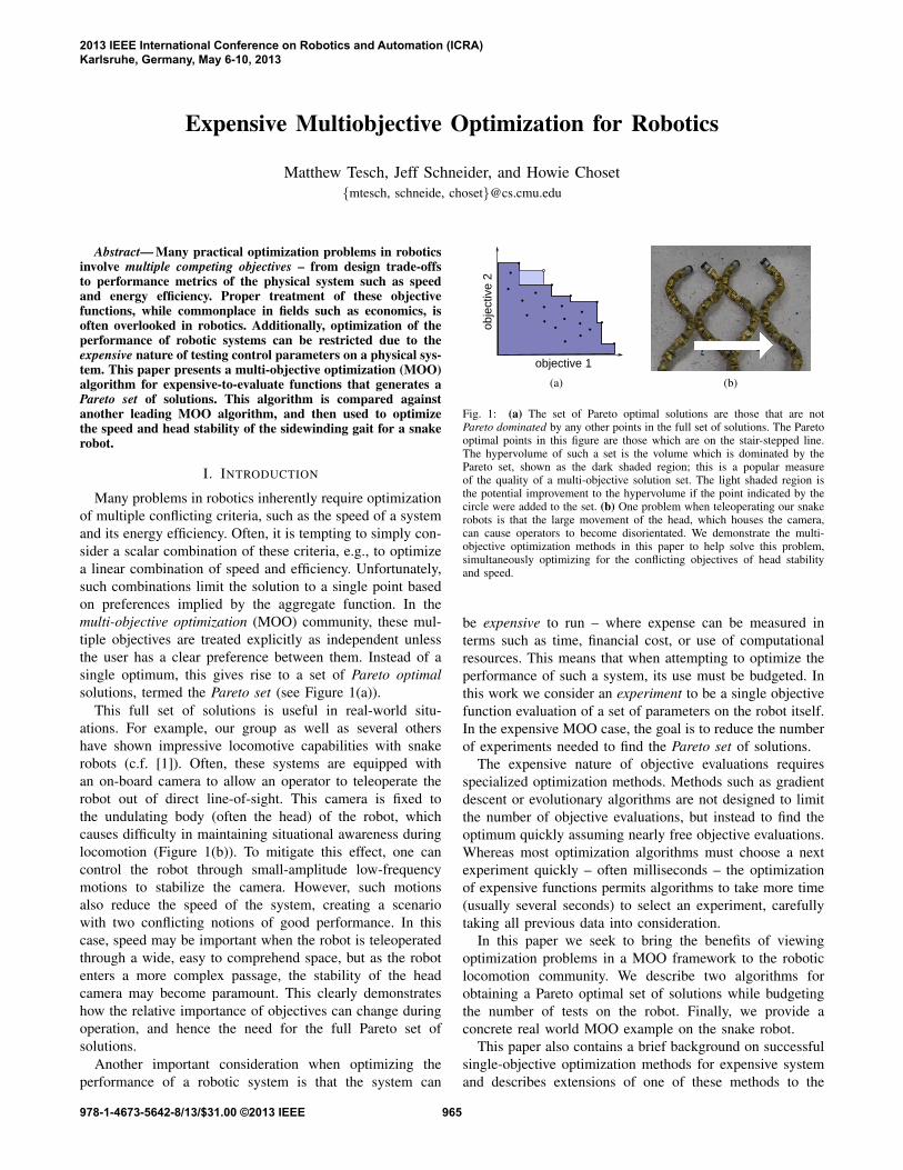
(a) (b)

Fig. 1: (a) The set of Pareto optimal solutions are those that are notPareto dominated by any other points in the full set of solutions. The Paretooptimal points in this figure are those which are on the stair-stepped line.The hypervolume of such a set is the volume which is dominated by thePareto set, shown as the dark shaded region; this is a popular measureof the quality of a multi-objective solution set. The light shaded region isthe potential improvement to the hypervolume if the point indicated by thecircle were added to the set. (b) One problem when teleoperating our snakerobots is that the large movement of the head, which houses the camera,can cause operators to become disorientated. We demonstrate the multi-objective optimization methods in this paper to help solve this problem,simultaneously optimizing for the conflicting objectives of head stabilityand speed.

be expensive to run – where expense can be measured interms such as time, financial cost, or use of computationalresources. This means that when attempting to optimize theperformance of such a system, its use must be budgeted. Inthis work we consider an experiment to be a single objectivefunction evaluation of a set of parameters on the robot itself.In the expensive MOO case, the goal is to reduce the numberof experiments needed to find the Pareto set of solutions.

The expensive nature of objective evaluations requiresspecialized optimization methods. Methods such as gradientdescent or evolutionary algorithms are not designed to limitthe number of objective evaluations, but instead to find theoptimum quickly assuming nearly free objective evaluations.Whereas most optimization algorithms must choose a nextexperiment quickly – often milliseconds – the optimizationof expensive functions permits algorithms to take more time(usually several seconds) to select an experiment, carefullytaking all previous data into consideration.

In this paper we seek to bring the benefits of viewingoptimization problems in a MOO framework to the roboticlocomotion community. We describe two algorithms forobtaining a Pareto optimal set of solutions while budgetingthe number of tests on the robot. Finally, we provide aconcrete real world MOO example on the snake robot.

This paper also contains a brief background on successfulsingle-objective optimization methods for expensive systemand describes extensions of one of these methods to the

2013 IEEE International Conference on Robotics and Automation (ICRA)Karlsruhe, Germany, May 6-10, 2013

978-1-4673-5642-8/13/$31.00 ©2013 IEEE 965

multi-objective case. We compare two MOO algorithms on aset of test functions, and finally, we seek to improve the headstability of our snake robot during execution of a sidewindinggait while simultaneously maximizing speed. The novelcontributions in this work include description, demonstration,and validation of an MOO algorithm based on the expectedimprovement in hypervolume [2], the first known applicationof MOO techniques to the robotics domain, and optimizationof the combined locomotive speed and head stability of oursnake robot system.

II. RELATED WORK

A. Expensive Black-Box Optimization

Expensive functions, or those for which evaluations takesignificant resources (time, money, computation, etc.), oftenalso fall in the category of black-box functions (those whichprovide no gradient or derivative information when sampled).Furthermore, these functions need not have guarantees ofconvexity or linearity; one must search for a global optimumover a function which is in all likelihood nonlinear andnon-convex. Optimization of such functions by many stan-dard techniques is ineffective; for example, gradient-ascentapproaches would require a number of samples around asampled point to find a (potentially unstable) approximationto the gradient. For expensive function evaluations this isimpractical (especially in higher dimensions) for a singlepoint/gradient sample.

This has motivated the development of a class of “gra-dient free” optimization techniques; these include local ap-proaches, such as a Nelder-Mead simplex search (c.f. [3]),and global approaches such as genetic algorithms [4] or sim-ulated annealing [5]. Naturally, a globally optimal solutionis preferred to a locally optimal one, but unfortunately mostmethods which search for such global optima require a largenumber of function evaluations. Again, this is prohibitive ifthese evaluations are expensive.

To address the particular challenges of expensive black-box optimization, a group of techniques is based on theidea of predicting the entire unknown expensive functionfrom limited sampled data. These surrogate function-basedsequential experiment selection methods rely on a functionregression method, usually a Gaussian process [6], to es-timate the true objective function after each subsequent ex-pensive function evaluation. The information provided by thesurrogate is then used to intelligently select parameters forfuture experiments. These regression methods often providea measure of the uncertainty of their estimate which canbe used in conjunction with the estimated objective functionvalue to make more informed decisions. An excellent surveyon this subject is given by Jones [7], and more recent worksuch as [8] continues to demonstrate new applications.

In our previous work [9], we have used these expensiveglobal optimization methods (in particular efficient globaloptimization, or EGO [10]) to optimize the performance ofthe snake robots discussed in this paper. To this point onlysingle-objective optimization problems have been consid-ered. Locomotion with snake robots serves as an exemplary

application of surrogate function optimization techniquesbecause each “experiment” with the snake robot can takeseveral minutes, and provides no gradient information (fittingthe “black box” description).

B. Multi-Objective Optimization

The notion of optimality that is embraced in the fieldof multi-objective optimization is that of a set of Paretooptimal solutions. This set, named after economist VilfredoPareto, includes all solutions which cannot be improved inone objective without a corresponding decrease in another. Inparticular, a point in objective space a is said to dominate b,written a � b or b ≺ a, if a is at least as good in everyobjective, and better in at least one. The Pareto optimalsubset of a collection of points P is {p ∈ P | ∀ q ∈ P, (p ∼q)∨ (p � q)}. For detailed coverage of these ideas, see [11].

This notion of Pareto optimality allows us to define thebest set of parameters given no particular relative importanceof the objectives. Once knowledge of this optimal set isobtained, it is straightforward to select the best parametersfor any given objective trade-offs or constraints. Findingsuch optimal sets has been important for a number ofreal world applications, including modeling grasshopperforaging behavior [12], rehabilitation of water distributionnetworks [13], design of airfoils [14], and optimization ofspacecraft trajectories [15].

However, finding these sets of optimal points requiresspecialized optimization methods. For cases where the ob-jective functions are linear, the NISE method [16] has beendeveloped to converge quickly on a good approximation ofthe Pareto set, even in problems of very high dimensions.Multiobjective simplex methods such as [17], which extendthe single-objective linear constrained optimization simplexmethod1 developed in 1947 [18], provide exact solutions forthe Pareto optimal set for linear objective functions.

For nonlinear cases there are also a number of methods;perhaps the most popular is the Non-dominated Sorting Ge-netic Algorithm II (NSGA-II) [19]. This empirically has beenshown to produce good results which are well distributedover the Pareto front – the Pareto optimal set given inobjective space coordinates.

C. Expensive MOO

In the case of expensive optimization for multiple ob-jectives, there is significantly less literature on identifyingthe Pareto set; the evolutionary methods used in standardMOO are most appropriate when samples are cheap andparameter and objective spaces are very high dimensional.Most expensive MOO approaches attempt to extend suc-cessful single objective expensive optimization techniques.One set of techniques create a single aggregate objectivefunction at each step, and choose to optimize this function;this approach is taken by ParEGO [20], where the aggregateis a weighted combination of individual objectives as terms in

1Note that this simple method differs from the Nelder Mead constrainednonlinear optimization method.

966

an augmented Tchebycheff function, and the single objectiveoptimization method used is Jones’ EGO algorithm.

Other approaches attempt to work in the full objectivespace rather than simplifying the problem to one objective.For example, Keane [21] attempts to directly measure themultivariate expected improvement of a point – how muchthe hypervolume of the Pareto front increases (Figure 1(a)).The expression Keane presents is a simplification of thetrue quantity and only measures improvement as an increasefrom a single point on the Pareto front; Emmerich et al. [2]redefine this improvement more rigorously (yet are still ableto find a closed-form expression) using Lebesgue integrationon a partition of the objective space.

D. Snake Robots

This work was motivated by the goal of improving thelocomotive capabilities of snake robots, especially those ofthe latest generation in our lab [22]. These robots havedemonstrated impressive locomotive capabilities, and withtheir small diameter of 10 cm they can fit into small channelsand spaces too confined for other mechanisms. Much liketheir biological counterparts they use cyclic control trajec-tories called gaits to move across relatively regular terrain,such as a flat expanse of grass, a roughly uniform diameterpole, or a regular grid of poles.

Although the space of cyclic controls is infinite, Choset’srobots are usually controlled by motions within a finitedimensional constrained control trajectory subspace (the gaitmodel described in [1]). This model, defined by

α(n, t) =

{βeven +Aeven sin(θ), n = even,βodd +Aodd sin(θ + δ), n = odd,

(1)

θ =

(dθ

dnn+

dθ

dtt

), (2)

is general enough to command the snake to slither, sidewind,roll in an arc, wrap around a tree or pole in a helix andclimb, turn in place, and traverse via many other motions.Similar controllers have been used by other researchers (c.f.[23], [24]). In this paper, we consider the optimization ofan augmented sidewinding gait, based this equation withrestrictions on the set of free parameters (β, A, etc.).

One difficulty with optimizing an objective like the stabil-ity of the head module during a gait is that there is no simple,accurate motion model for these robots due to their frequentcollisions with the ground and multiple simultaneous slidingcontacts. This requires one to actually run experiments ona physical system to reliably sample such an objective,which motivates the use of expensive optimization techniquesdescribed above.

III. OPTIMIZATION METHOD OVERVIEW

We first describe the single-objective precursors to theMOO algorithms that are the focus of the paper. Althoughan algorithm based on the optimization of Emmerich et al.’sexpression for the expected hypervolume improvement isdescribed below, we also implement the ParEGO aggregate

0 1 2 3 4 5 6 7 8 9 10−3

−2

−1

0

1

2

3

(a)0 1 2 3 4 5 6 7 8 9 10

−2.5

−2

−1.5

−1

−0.5

0

0.5

1

1.5

2

2.5

(b)

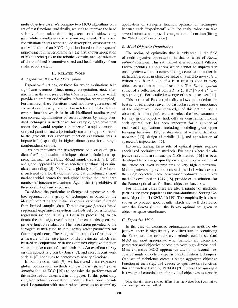
Fig. 2: (a): A surrogate function (dark line) interpolates sampled points ofan unknown underlying function (dotted red line). The surrogate quantifiesuncertainty in its prediction, as shown by the shaded region.(b): Experi-ment selection metrics such as probability of improvement and expectedimprovement consider the predictive distribution at a potential sample pointx (vertical line), compared to the best previous sample (horizontal line).

function optimization method for purposes of comparisonand verification. We note before continuing that we usethe convention of maximizing a reward function rather thanminimizing; this differs from much of the optimizationliterature referenced, but aligns with our goal of improvingrobot performance.

A. Expensive Single Objective Optimization

The expensive single optimization methods that underlythis work are global, constrained methods. Formally, givena parameter space X ⊂ Rn and a objective function f : X →R, they search for argmaxx∈X f(x). As it is expensive toobtain samples of f(x), there is a limit to the number oftimes f can be sampled.

As described above, a common and successful approach toexpensive optimization task involves the use of a nonlinearsurrogate function fit to the sampled data points, as shown inFigure 2(a). Such algorithms are summarized in the followingsteps:

1) Sample a set of initial points (often randomly or witha Latin hypercube experimental design)

2) Fit a surrogate to the sampled points3) Select the next sample location by optimizing a metric4) Repeat steps 2-3 until convergenceThe central challenge is the determination of the fitness

metric which is optimized in step 3 to select subsequentsample locations. This metric must balance exploration(sampling in unknown regions) and exploitation (samplingin known good regions) during the optimization. Neitherextreme (choosing the current maximum of the surrogateor sampling purely based on uncertainty, such as [25])result in methods which converge to the optimum efficiently.To improve the quality of search, the uncertainty of theestimated function value should be used in conjunction withthat estimated value.

To this end, simple approaches may select subsequentsamples based on a weighted sum of the estimated functionand its error (c.f. IEMAX [26]). Another approach that incor-porates a natural trade-off is to maximize the probability ofimprovement [27], [28]. For a given test point, the probabilityof improvement is the integral of the tail of the predictivedistribution above the maximum value of the objective found

967

so far (Figure 2(b)). To be successful, these methods requiretuning parameters that explicitly balance exploration andexploitation.

We choose to use a more principled method to addressthis trade-off: the idea of expected improvement (EI) [29]popularized by Jones et al.’s efficient global optimization(EGO) algorithm [10]. Given a set of sampled values Y ,the improvement I(y∗) of a new sample at x with the valuey∗ is the increase in the maximum value of this set withthe addition of y∗. The expectation of this quantity overthe surrogate function’s predictive distribution at x, px(y),is given as

EI(x) = E[I(y)] (3)

=

∫ ∞max(Y )

(y −max(Y ))px(y) dy, (4)

and captures the intuitive idea of selecting the next sampleas the point which you expect to most improve your currentsolution (Figure 2(b)). This statistical measure automaticallybalances the trade-off between exploration and exploitationwithout requiring a tuning parameter.

B. Multiple Objective Extensions

As the expected improvement metric has been a success inexpensive single-objective optimization, the natural questionis whether it can be applied to the MOO case. In order toextend the EI metric, one must first define the notion of‘improvement’. In the single objective case, improvementhas a natural definition, because there is already a singleobjective f which is being optimized. The improvement ofa sampled value of y∗ over the set of sampled points Y issimply the increase in the maximum value of the resultingset, or

I(y∗) = max(y∗ −max(Y ), 0) (5)

In multi-objective optimization there is more than oneobjective, and the solution is not just a single point, butan entire Pareto set of points. To measure improvementin such a set, a valid metric must be devised to measurethe quality of such a set. One such metric is the set’shypervolume [30]. This is the volume in objective spacewhich is Pareto-dominated by at least one point in the Paretoset. A reference point in objective space must be selected todefine the lower bounds of this volume; this point should bechosen given prior knowledge of or an educated guess aboutthe minimum possible value of the objective functions (e.g.,the net displacement of a gait must always be greater thanor equal to 0).

The concept of the hypervolume indicator is illustrated fora two-dimensional objective space in Figure 1(a). This mea-sure has desirable properties; for example it is not affectedwhen a dominated point is added to a set of solutions, and theaddition of a non-dominated point always increases a set’shypervolume. Given a method to compute the hypervolumeHV of a solution set, improvement can be defined as

I(y∗) = HV(Y ∪ y∗)−HV(Y ). (6)

Although a simple closed-form solution has been derivedfor EI in the single objective case, E[I(y∗)] is not straightfor-ward when the improvement is measured in terms of hyper-volume; evaluating this for a given test point requires eithera multidimensional numerical integral, or the development ofan analytic form for this expectation. Fortunately, Emmerichet al. have provided the outline of a method to computethis quantity in closed form [2]. Because we are working inobjective space, this metric considers the joint improvementin all objectives simultaneously, trading off the benefits ofsampling a point which might improve one or the other.

Using hypervolume as the indicator of solution set qualityand finding an efficient computation of its expectation allowsus to use machinery from the single objective case foroptimization with multiple objectives. Our multi-objectiveoptimization algorithm using the expected improvement inhypervolume (EIHV) metric can be summarized in a formparallel to that of surrogate-based single objective algo-rithms:

1) Sample the objectives at a set of initial points2) Fit a surrogate to the sampled points for each objective

function3) Select the next sample location by selecting the sample

with the largest EIHV value4) Repeat steps 2-3 until convergence

C. Limitations and Implementation Details

When implementing surrogate-function based algorithms,a number of issues can arise. Most importantly, these meth-ods rely on the function regression method to provide a rea-sonable estimate of the objective and the uncertainty of thatestimate. We use Gaussian processes (GPs) as this regressionmethod, which can lead to a number of pitfalls. From ourexperience, we have a number of recommendations. First, theuse of an existing package, such as the GPML MATLABlibrary [31], can greatly reduce initial time and effort ofimplementation. Next, when fitting a surface, it is importantto carefully tune the hyperparameters that describe the GP toobtain a realistic and non-trivial fit. As recommended by [6],we find hyperparameters that maximize the log likelihood ofthe data. This is done via a large number of line searchoptimizations in the hyperparameter space (using the GPMLpackage’s minimize function) from hundreds of randomseed points, including the best hyperparameter value foundin a previous fit.

To further improve the fit and reduce necessary manualinvolvement with the fitting process, we choose to run thishyperparameter selection process over a number of differentsets of covariance functions for the GP (effectively modelselection over a number of different function forms forregression). By using the log likelihood of the data as aselection metric, this allows the complexity of the model tomatch the complexity of the data. Initially, simple covariancefunctions are chosen; as the number of data points collected

968

increases, the complexity typically grows to match the trendsshown by the data.

In addition to obtaining a quality surrogate function fit, itis important to ensure the global maximum is found whenoptimizing the experiment selection metric. This functionis often highly irregular and strongly peaked. Taking thelogarithm can ensure a more numerically stable optimization.Also, we advise many random restarts of your favorite built-in optimization algorithm to ensure that the space is wellcovered. As this optimization determines the quality of thepoint selected, it is important to spend time on this step, bothduring implementation as well as when running the code toselect experiments.

Finally, the effectiveness of these methods is restricted tofairly low-dimensional spaces. The authors usually work withparameter spaces from 2-8 dimensions, but have had successup to 20 depending on the objective function complexity.The limitations are driven by the ease and robustness offitting a GP in higher dimensions and the reliability of theoptimization of the selection metric in those spaces.

IV. TEST RESULTS

The primary motivation for the careful experiment selec-tion methods described herein is the expensive nature of test-ing the performance of physical robotic systems. Therefore tojustify the selection of one algorithm to use for optimizationof a physical system, we ran a more extensive comparisonon two simple analytic functions. This also allowed us totest algorithm implementations, and ensure they functionedas expected.

Many of the multi-objective test functions in the litera-ture are particularly designed to confound existing multi-objective evolutionary algorithms (MOEAs), and thereforeinvolve large high-dimensional parameter spaces with manyseparated Pareto set regions. The low dimensional analogues,when they exist, are trivial surfaces that do not provide fora reasonable evaluation of the optimization algorithms wewere considering.

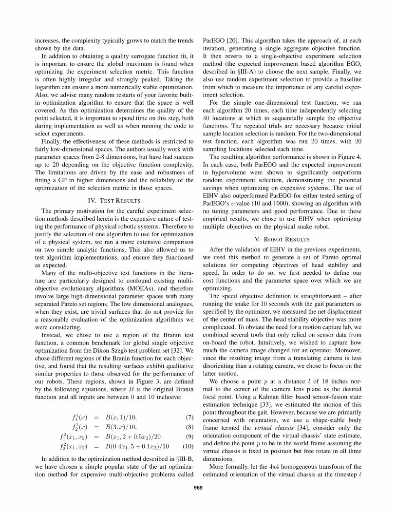
Instead, we chose to use a region of the Branin testfunction, a common benchmark for global single objectiveoptimization from the Dixon-Szego test problem set [32]. Wechose different regions of the Branin function for each objec-tive, and found that the resulting surfaces exhibit qualitativesimilar properties to those observed for the performance ofour robots. These regions, shown in Figure 3, are definedby the following equations, where B is the original Braninfunction and all inputs are between 0 and 10 inclusive:

f11 (x) = B(x, 1)/10, (7)f12 (x) = B(3, x)/10, (8)

f21 (x1, x2) = B(x1, 2 + 0.5x2)/20 (9)f22 (x1, x2) = B(0.4x1, 5 + 0.1x2)/10 (10)

In addition to the optimization method described in §III-B,we have chosen a simple popular state of the art optimiza-tion method for expensive multi-objective problems called

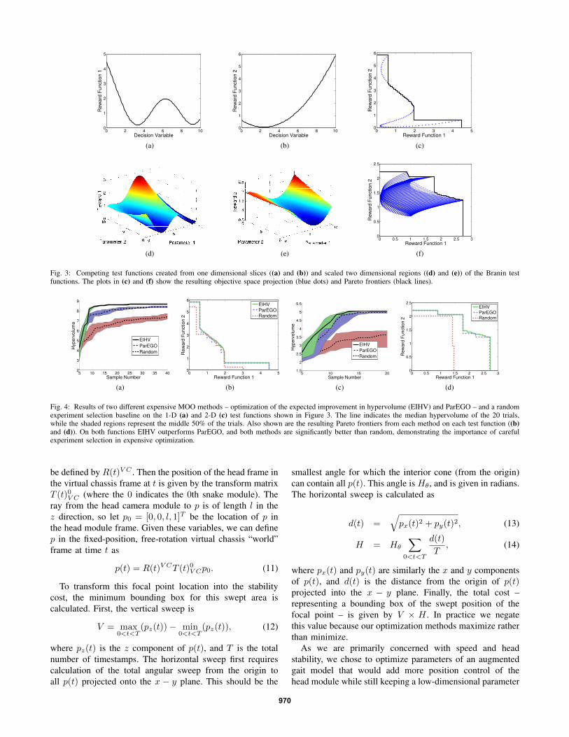
ParEGO [20]. This algorithm takes the approach of, at eachiteration, generating a single aggregate objective function.It then reverts to a single-objective experiment selectionmethod (the expected improvement based algorithm EGO,described in §III-A) to choose the next sample. Finally, wealso use random experiment selection to provide a baselinefrom which to measure the importance of any careful exper-iment selection.

For the simple one-dimensional test function, we raneach algorithm 20 times, each time independently selecting40 locations at which to sequentially sample the objectivefunctions. The repeated trials are necessary because initialsample location selection is random. For the two-dimensionaltest function, each algorithm was run 20 times, with 20sampling locations selected each time.

The resulting algorithm performance is shown in Figure 4.In each case, both ParEGO and the expected improvementin hypervolume were shown to significantly outperformrandom experiment selection, demonstrating the potentialsavings when optimizing on expensive systems. The use ofEIHV also outperformed ParEGO for either tested setting ofParEGO’s s-value (10 and 1000), showing an algorithm withno tuning parameters and good performance. Due to theseempirical results, we chose to use EIHV when optimizingmultiple objectives on the physical snake robot.

V. ROBOT RESULTS

After the validation of EIHV in the previous experiments,we used this method to generate a set of Pareto optimalsolutions for competing objectives of head stability andspeed. In order to do so, we first needed to define ourcost functions and the parameter space over which we areoptimizing.

The speed objective definition is straightforward – afterrunning the snake for 10 seconds with the gait parameters asspecified by the optimizer, we measured the net displacementof the center of mass. The head stability objective was morecomplicated. To obviate the need for a motion capture lab, wecombined several tools that only relied on sensor data fromon-board the robot. Intuitively, we wished to capture howmuch the camera image changed for an operator. Moreover,since the resulting image from a translating camera is lessdisorienting than a rotating camera, we chose to focus on thelatter motion.

We choose a point p at a distance l of 18 inches nor-mal to the center of the camera lens plane as the desiredfocal point. Using a Kalman filter based sensor-fusion stateestimation technique [33], we estimated the motion of thispoint throughout the gait. However, because we are primarilyconcerned with orientation, we use a shape-stable bodyframe termed the virtual chassis [34], consider only theorientation component of the virtual chassis’ state estimate,and define the point p to be in the world frame assuming thevirtual chassis is fixed in position but free rotate in all threedimensions.

More formally, let the 4x4 homogeneous transform of theestimated orientation of the virtual chassis at the timestep t

969

0 2 4 6 8 100

1

2

3

4

5

Decision Variable

Re

wa

rd F

un

ctio

n 1

(a)

0 2 4 6 8 100

1

2

3

4

5

6

Decision Variable

Re

wa

rd F

un

ctio

n 2

(b)

0 1 2 3 4 50

1

2

3

4

5

6

Reward Function 1

Rew

ard

Function 2

(c)

(d) (e)

0 0.5 1 1.5 2 2.5 30

0.5

1

1.5

2

2.5

Reward Function 1

Rew

ard

Function 2

(f)

Fig. 3: Competing test functions created from one dimensional slices ((a) and (b)) and scaled two dimensional regions ((d) and (e)) of the Branin testfunctions. The plots in (c) and (f) show the resulting objective space projection (blue dots) and Pareto frontiers (black lines).

5 10 15 20 25 30 35 402

3

4

5

6

7

8

9

Sample Number

Hyperv

olu

me

EIHV

ParEGO

Random

(a)

0 1 2 3 4 50

1

2

3

4

5

6

Reward Function 1

Re

wa

rd F

un

ctio

n 2

EIHV

ParEGO

Random

(b)

5 10 15 201.5

2

2.5

3

3.5

4

4.5

5

5.5

Sample Number

Hyperv

olu

me

EIHV

ParEGO

Random

(c)

0 0.5 1 1.5 2 2.5 30

0.5

1

1.5

2

2.5

Reward Function 1

Re

wa

rd F

un

ctio

n 2

EIHV

ParEGO

Random

(d)

Fig. 4: Results of two different expensive MOO methods – optimization of the expected improvement in hypervolume (EIHV) and ParEGO – and a randomexperiment selection baseline on the 1-D (a) and 2-D (c) test functions shown in Figure 3. The line indicates the median hypervolume of the 20 trials,while the shaded regions represent the middle 50% of the trials. Also shown are the resulting Pareto frontiers from each method on each test function ((b)and (d)). On both functions EIHV outperforms ParEGO, and both methods are significantly better than random, demonstrating the importance of carefulexperiment selection in expensive optimization.

be defined by R(t)V C . Then the position of the head frame inthe virtual chassis frame at t is given by the transform matrixT (t)0V C (where the 0 indicates the 0th snake module). Theray from the head camera module to p is of length l in thez direction, so let p0 = [0, 0, l, 1]T be the location of p inthe head module frame. Given these variables, we can definep in the fixed-position, free-rotation virtual chassis “world”frame at time t as

p(t) = R(t)V CT (t)0V Cp0. (11)

To transform this focal point location into the stabilitycost, the minimum bounding box for this swept area iscalculated. First, the vertical sweep is

V = max0<t<T

(pz(t))− min0<t<T

(pz(t)), (12)

where pz(t) is the z component of p(t), and T is the totalnumber of timestamps. The horizontal sweep first requirescalculation of the total angular sweep from the origin toall p(t) projected onto the x − y plane. This should be the

smallest angle for which the interior cone (from the origin)can contain all p(t). This angle is Hθ, and is given in radians.The horizontal sweep is calculated as

d(t) =√px(t)2 + py(t)2, (13)

H = Hθ

∑0<t<T

d(t)

T, (14)

where px(t) and py(t) are similarly the x and y componentsof p(t), and d(t) is the distance from the origin of p(t)projected into the x − y plane. Finally, the total cost –representing a bounding box of the swept position of thefocal point – is given by V × H . In practice we negatethis value because our optimization methods maximize ratherthan minimize.

As we are primarily concerned with speed and headstability, we chose to optimize parameters of an augmentedgait model that would add more position control of thehead module while still keeping a low-dimensional parameter

970

00.5

1 0

0.5

1

−80

−60

−40

−20

0

HeadOffsetAmplitude

Sta

bili

ty

(a) 11th sample

00.5

1 0

0.5

1

−80

−60

−40

−20

0

HeadOffsetAmplitude

Sta

bili

ty

(b) 18th sample

00.5

1 0

0.5

1

−80

−60

−40

−20

0

HeadOffsetAmplitude

Sta

bili

ty

(c) 25th sample

00.5

1 0

0.5

1

0

20

40

60

HeadOffsetAmplitude

Speed

(d) 11th sample

00.5

1 0

0.5

1

0

20

40

60

HeadOffsetAmplitude

Speed

(e) 18th sample

00.5

1 0

0.5

1

0

20

40

60

HeadOffsetAmplitude

Speed

(f) 25th sample

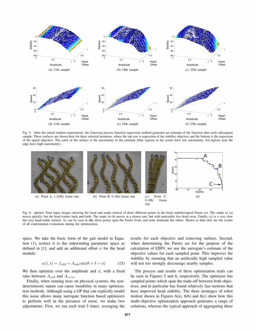
Fig. 5: After the initial random experiments, the Gaussian process function regression method generates an estimate of the function after each subsequentsample. These surfaces are shown here for three selected iterations, where the top row is regression of the stability objective and the bottom is the regressionof the speed objective. The color of the surface is the uncertainty in the estimate (blue regions in the center have low uncertainty, red regions near theedge have high uncertainty).

(a) Point A, 1.25Hz frame rate (b) Point B, 0.4Hz frame rate (c) Point C,0.4Hz framerate

−80 −60 −40 −20 00

10

20

30

40

50

Stability

Spe

ed

A

B

C

(d)

Fig. 6: (a)-(c): Time lapse images showing the head and snake motion of three different points in the head stability/speed Pareto set. The snake in (a)moves quickly, but the head rotates back and forth. The snake in (b) moves at a slower rate, but with noticeably less head sway. Finally, (c) is a very slowbut very head-stable motion. As can be seen in (d), these points span the Pareto front, and none dominate the others. Shown as blue dots are the resultsof all experimental evaluations during the optimization.

space. We take the basic form of the gait model in Equa-tion (1), restrict it to the sidewinding parameter space asdefined in [1], and add an additional offset φ for the headmodule:

α(1, t) = βodd +Aodd sin(θ + δ + φ) (15)

We then optimize over the amplitude and φ, with a fixedratio between Aodd and Aeven.

Finally, when running tests on physical systems, the non-deterministic nature can cause instability in many optimiza-tion methods. Although using a GP that can explicitly modelthis noise allows many surrogate function based optimizersto perform well in the presence of noise, we make twoadjustments. First, we run each trial 5 times, averaging the

results for each objective and removing outliers. Second,when determining the Pareto set for the purpose of thecalculation of EIHV, we use the surrogate’s estimate of theobjective values for each sampled point. This improves thestability by ensuring that an artificially high sampled valuewill not too strongly discourage nearby samples.

The process and results of these optimization trials canbe seen in Figures 5 and 6, respectively. The optimizer hassampled points which span the trade-off between both objec-tives, and in particular has found relatively fast motions thathave improved head stability. The three montages of robotmotion shown in Figures 6(a), 6(b) and 6(c) show how thismulti-objective optimization approach generates a range ofsolutions, whereas the typical approach of aggregating these

971

objectives would only have found one of these solutions.

VI. CONCLUSIONS AND FUTURE WORK

Multi-objective optimization is often a reasonable alter-native to creating a single aggregate objective in the caseof competing system performance objectives. This is a casewhich comes up frequently in robotics as well as manyother fields such as design, decision theory, and economics.Instead, a Pareto optimal set should be found, which con-tains all solutions which are not dominated, or completelyoutperformed, by another solution. The generation of Paretooptimal solutions sets is especially difficult when samplingthe performance of a system is expensive, but once accom-plished these solutions can be selected from to provide real-time trade-offs between objectives.

In this paper, we have created and tested a MOO approachbased on maximization of the expected improvement inhypervolume of the Pareto set. We have compared this to aleading MOO algorithm, ParEGO, on multiple test functions.Finally, we have applied the former algorithm to a practicalapplication, the task of finding snake robot gait parametersfor fast and head-stable sidewinding. This application re-quired care to reduce the effect of noisy evaluations on theoptimization performance as well as the creation of a head-stability cost function from recent state-estimation techniquesfor the robot.

Future work involves testing these methods with higherdimensional parameter spaces and use of these methods onother robotic systems. In addition, the explicit handling ofnoisy objective evaluations and guarantees of convergence toa dense covering of the full Pareto optimal solution set areopen problems. Both of these should be addressed in orderto give potential adopters more confidence in the results ofthese methods.

REFERENCES

[1] M. Tesch, K. Lipkin, I. Brown, R. Hatton, A. Peck, J. Rembisz,and H. Choset, “Parameterized and Scripted Gaits for Modular SnakeRobots,” Advanced Robotics, vol. 23, no. 9, pp. 1131–1158, Jun. 2009.

[2] M. Emmerich and J.-w. Klinkenberg, “The computation of the ex-pected improvement in dominated hypervolume of Pareto front ap-proximations,” Leiden Institute for Advanced Computer Science, Tech.Rep. 1, 2008.

[3] J. A. Nelder and R. Mead, “A Simplex Method for Function Mini-mization,” The Computer Journal, vol. 7, no. 4, Jan. 1965.

[4] W. Banzhaf, P. Nordin, R. E. Keller, and F. D. Francone, GeneticProgramming: An Introduction. Morgan Kaufmann, 1997.

[5] S. Kirkpatrick, C. D. Gelatt Jr., and M. P. Vecchi, “Optimization bySimulated Annealing,” Science, vol. 220, no. 4598, pp. 671–680, 1983.

[6] C. E. Rasmussen and C. K. I. Williams, Gaussian Processes forMachine Learning. The MIT Press, 2006.

[7] D. R. Jones, “A taxonomy of global optimization methods based onresponse surfaces,” Journal of Global Optimization, vol. 21, no. 4, pp.345–383, 2001.

[8] J. Snoek, H. Larochelle, and R. P. Adams, “Practical Bayesian Opti-mization of Machine Learning Algorithms,” ArXiv e-prints, 2012.

[9] M. Tesch, J. Schneider, and H. Choset, “Using Response Surfaces andExpected Improvement to Optimize Snake Robot Gait Parameters,” inInternational Conference on Intelligent Robots and Systems. SanFrancisco: IEEE/RSJ, 2011.

[10] D. R. Jones, M. Schonlau, and W. J. Welch, “Efficient GlobalOptimization of Expensive Black-Box Functions,” Journal of GlobalOptimization, vol. 13, no. 4, 1998.

[11] J. L. Cohon, Multiobjective Programming and Planning. CourierDover Publications, 2004.

[12] K. D. Rothley, O. J. Schmitx, and J. L. Cohon, “Foraging to balanceconflicting demands : novel insights from grasshoppers under preda-tion risk,” Behavioral Ecology, vol. 8, no. 5, pp. 551–559, 1997.

[13] P. B. Cheung, L. F. Reis, K. T. Formiga, F. H. Chaudhry, andW. G. Ticona, “Multiobjective evolutionary algorithms applied to therehabilitation of a water distribution system: A comparative study,”in Int. Conf. Evol. Multicriterion Optimization, C. M. Fonseca andE. Al., Eds. Berlin, Germany: Springer-Verlag, 2003, pp. 662–676.

[14] B. Naujoks, L. Willmes, T. Back, and W. Haase, “Evaluating Multi-criteria Evolutionary Algorithms for Airfoil Optimisation,” LECTURENOTES IN COMPUTER SCIENCE, no. 2439, pp. 841–850, 2003.

[15] V. Coverstone-Carroll, “Optimal multi-objective low-thrust spacecrafttrajectories,” Computer Methods in Applied Mechanics and Engineer-ing, vol. 186, no. 2-4, pp. 387–402, Jun. 2000.

[16] R. S. Solanki, P. A. Appino, and J. L. Cohon, “Theory and Method-ology Approximating the noninferior set in multiobjective linearprogramming problems,” European Journal Of Operational Research,vol. 68, pp. 356–373, 1993.

[17] M. Zeleny, Linear Multiobjective Programming. Springer-Verlag,1974.

[18] G. B. Dantzig, “Programming in a Linear Structure,” Comptroller,USAF, Washington, D.C., Tech. Rep., 1948.

[19] K. Deb, A. Pratap, S. Agarwal, and T. Meyarivan, “A Fast ElitistMulti-Objective Genetic Algorithm: NSGA-II,” IEEE Transactions onEvolutionary Computation, vol. 6, pp. 182—-197, 2000.

[20] J. Knowles, “ParEGO: a hybrid algorithm with on-line landscapeapproximation for expensive multiobjective optimization problems,”IEEE Transactions on Evolutionary Computation, vol. 10, no. 1, pp.50–66, Feb. 2006.

[21] A. J. KEANE, “Statistical improvement criteria for use in multiobjec-tive design optimization,” AIAA journal, vol. 44, no. 4, pp. 879–891,2006.

[22] C. Wright, A. Buchan, B. Brown, J. Geist, M. Schwerin, D. Rollinson,M. Tesch, and H. Choset, “Design and Architecture of the UnifiedModular Snake Robot,” in 2012 IEEE International Conference onRobotics and Automation, St. Paul, MN, 2012.

[23] J. Gonzalez-Gomez, H. Zhang, E. Boemo, and J. Zhang, “Locomotioncapabilities of a modular robot with eight pitch-yaw-connecting mod-ules,” in 9th international conference on climbing and walking robots.Citeseer, 2006.

[24] A. Kuwada, S. Wakimoto, K. Suzumori, and Y. Adomi, “Automaticpipe negotiation control for snake-like robot,” 2008 IEEE/ASMEInternational Conference on Advanced Intelligent Mechatronics, no.438, pp. 558–563, Jul. 2008.

[25] J. M. Bernardo, “Expected Information as Expected Utility,” TheAnnals of Statistics, vol. 7, no. 3, pp. 686–690, May 1979.

[26] A. W. Moore and J. Schneider, “Memory-based stochastic optimiza-tion,” Advances in Neural Information Processing Systems, pp. 1066–1072, 1996.

[27] H. J. Kushner, “A new method for locating the maximum point of anarbitrary multipeak curve in the presence of noise.” Journal of BasicEngineering, vol. 86, pp. 97–106, 1964.

[28] A. Zilinskas, “A review of statistical models for global optimization,”Journal of Global Optimization, vol. 2, no. 2, pp. 145–153, Jun. 1992.

[29] J. Mockus, V. Tiesis, and A. Zilinskas, “The application of Bayesianmethods for seeking the extremum,” Towards Global Optimization,vol. 2, pp. 117–129, 1978.

[30] E. Zitzler and L. Thiele, “Multiobjective Optimization Using Evolu-tionary Algorithms - A Comparative Case Study,” pp. 292–304, Sep.1998.

[31] C. E. Rasmussen and C. K. I. Williams, “Gaussian Processes forMachine Learning.” [Online]. Available: http://www.gaussianprocess.org/gpml/code/gpml-matlab.tar.gz

[32] L. Dixon and G. Szego, “The global optimization problem: an intro-duction,” Towards Global Optimization, vol. 2, pp. 1 – 15, 1978.

[33] D. Rollinson, A. Buchan, and H. Choset, “State Estimation for SnakeRobots,” IEEE International Conference on Intelligent Robots andSystems, pp. 1075–1080, 2011.

[34] D. Rollinson and H. Choset, “Virtual Chassis for Snake Robots,”IEEE International Conference on Intelligent Robots and Systems(accepted), 2011.

972