multiobjective optimization methods -...
TRANSCRIPT

Multiobjective optimization
methods
Jussi Hakanen
Post-doctoral researcher [email protected]
spring 2014 TIES483 Nonlinear optimization

No-preference methods
DM not available (e.g. online optimization)
No preference information available
Compute some PO solution
Do not take into account which problem is
solved
Fast methods
– One PO solution is enough
– No communication with the DM

Method of global criterion
min𝑥∈𝑆
𝑓𝑖 𝑥 − 𝑧𝑖∗ 𝑝𝑘
𝑖=1
1/𝑝
Distance to the ideal objective vector is
minimized
Different metrics can be used, e.g. Lp metric
where 1 ≤ p ≤ ∞
A single objective optimization problem is solved

Method of global criterion
L1 metric
L2 metric
L∞ metric
Ideal objective
vector

Method of global criterion
When p=∞, maximum metric → nonsmooth
optimization problem
If p < ∞, the solution obtained is PO
If p = ∞, the solution obtained is weakly PO

A posteriori methods
Idea: 1) compute different PO solutions,
2) the DM selects the most preferred one
Approximation of the PO set (or part of it) is
approximated
Benefits
– Well suited for problems with 2 objectives since the
PO solutions can be easily visualized for the DM
– Understanding of the whole PO set

A posteriori methods
Drawbacks
– Approximating the PO set often time consuming
– DM has to choose the most preferred solution
among large number of solutions
– Visualization of the solutions for high number of
objectives

Weighting method
min𝑥∈𝑆
𝑤𝑖𝑓𝑖(𝑥)𝑘𝑖=1 ,
where 𝑤𝑖𝑘𝑖=1 = 1, 𝑤𝑖 ≥ 0, 𝑖 = 1,… , 𝑘
A weighted sum of the objectives is optimized
different PO solutions can be obtained by
changing the weights wi
One of the most well-known methods
– Gass & Saaty (1955), Zadeh (1963)

Weighting method
Benefits
– Solution obtained with positive weights is PO
– Easy to solve (simple objective function, no
additional constraints)
Drawbacks
– Can’t find solutions from non-convex parts of the
PO set
– PO solution obtained does not necessarily reflect
the preferences

Convex / non-convex PO set
Weights = slope of the level set of the objective function – Slope changes by changing the weights
Non-convex part can’t be reached with any weights!
f1, min
f2,
min
f1, min
f2,
min
w1=0.5, w2=0.5
w1=1/3, w2=2/3
convex PO set Non-convex PO set

Weighting method
Result1: The solution given by the weighting method is weakly PO
Result2: The solution given by the weighting method is PO if all the weights are strictly positive
Result3: Let 𝑥∗ be a PO solution of a convex multiobjective optimization problem. Then there exists a weighting vector 𝑤 = 𝑤1, … , 𝑤𝑘
𝑇 such that 𝑥∗ is the solution obtained with the weighting method.

Example
Where to go for a vacation (adopted from Prof. Pekka Korhonen)
The place with the best value for the objective function is the worst with respect to the most important objective!
Price Hiking Fishing Surfing
A 1 10 10 10
B 5 5 5 5
C 10 1 1 1
weight
Price Hiking Fishing Surfing
A 1 10 10 10
B 5 5 5 5
C 10 1 1 1
weight 0,4 0,2 0,2 0,2
Price Hiking Fishing Surfing Max
A 1 10 10 10 6,4
B 5 5 5 5 5
C 10 1 1 1 4,6
weight 0,4 0,2 0,2 0,2

ε-constraint method
min𝑥∈𝑆
𝑓𝑗(𝑥) 𝑠. 𝑡. 𝑓𝑖 𝑥 ≤ 𝜖𝑖 , ∀ 𝑖 ≠ 𝑗
Choose one of the objectives to be
optimized, give other objectives an upper
bound and consider them as constraints
Different PO solutions can be obtained by
changing the bounds and/or the objective to be
optimized
Haimes, Lasdon & Wismer (1971)

ε-constraint method
PO solutions for
different upper
bounds for 𝑓2
– ε1: no solutions
– ε2: z2
– ε3: z3
– ε4: z4
Fro
m M
iett
ine
n: N
on
line
ar
op
tim
iza
tio
n, 2
00
7 (
in F
inn
ish
)

ε-constraint method
Benefits
– Every PO solution can be found (also for non-
convex problems)
– Easy to implement
Drawbacks
– How to choose upper bounds?
• Does not necessarily give feasible solutions
– How to choose the objective to be optimized?

ε-constraint method
Result1: A solution obtained with the ε-
constraint method is weakly PO
Result2: A unique solution obtained with the ε-
constraint method is PO
Result3: A solution 𝑥∗ ∈ 𝑆 is PO if and only if it
is the solution given by the ε-constraint method
for every 𝑗 = 1,… , 𝑘 where 𝜖𝑖 = 𝑓𝑖 𝑥∗ , 𝑖 ≠ 𝑗.
(every PO solution can be found)

ε-constraint method
PO vs. weakly PO
– ε1: weakly PO
– ε2: PO
f1, min
f2,
min
ε1
ε2=f2(x*)
weakly PO
PO

Equally spaced PO solutions?
The weighting method:
change the weights
systematically
In the figure, PO solutions
are nearer to each other
towards the minimum of 𝑓2
How to obtain equally
spaced set? f1, min
f2,
min

Normal Boundary Intersection (NBI)
Find the extreme solutions of the PO set
Construct a plane passing through the extreme solutions; fix equally spaced points in the plane
Search orthogonal to the plane
f1, min
f2,
min

Normal Boundary Intersection (NBI)
Idea: produce equally spaced approximation of the PO set
Solutions are produced by solving
max𝑥∈𝑆
𝜆 𝑠. 𝑡. 𝑃𝑤 − 𝜆𝑃𝑒 = 𝑓 𝑥 − 𝑧∗,
where 𝑃 is a payoff table, 𝑤 is the vector of weights ( 𝑤𝑖 = 1,𝑤𝑖 ≥ 0𝑘
𝑖=1 ) and 𝑒 = 1,… , 1 𝑇
Das & Dennis, SIAM Journal of Optimization, 8, 1998
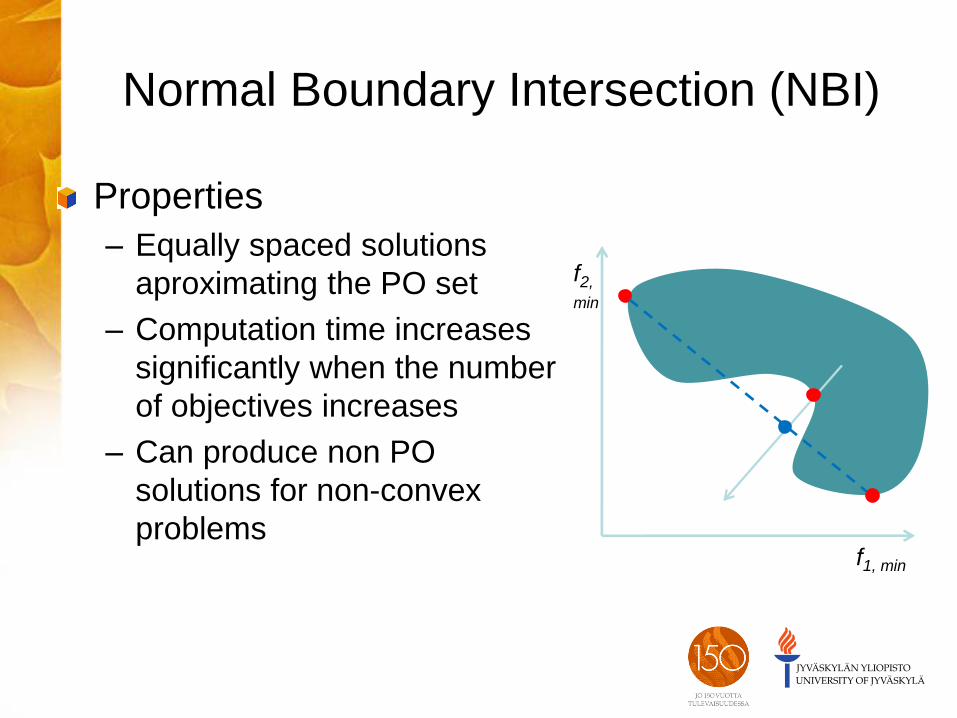
Normal Boundary Intersection (NBI)
Properties
– Equally spaced solutions
aproximating the PO set
– Computation time increases
significantly when the number
of objectives increases
– Can produce non PO
solutions for non-convex
problems f1, min
f2,
min

Equally spaced PO solutions?
The weighting method
f1, min
f2,
min
f1, min
f2,
min
Normal Boundary Intersection
NBI gives more equally spaced solutions

A priori methods
Idea: 1) ask first the preferences of the DM, 2) optimize using the preferences
Only such PO solutions are produced that are of interest to the DM
Benefits – Computed PO solutions are based on the preferences
of the DM (no ”unnecessary” solutions)
Drawbacks – It may be difficult for the DM to express preferences
before (s)he has seen any solutions

Lexicographic ordering
Order the objectives according to their importance
Optimize first w.r.t. to the most important one and continue optimizing the second most important one in the set of optimal solutions for the first one etc.
Requires the importance order from the DM before optimization
The solution obtained is PO

Lexicographic ordering
2 objectives: 1st
more important
Optimize w.r.t. 1st:
z1 and z2 obtained
Optimize w.r.t. 2nd:
choose better → z1
In practice, some
tolerance is used
for optimal values Fro
m M
iett
ine
n: N
on
line
ar
op
tim
iza
tio
n, 2
00
7 (
in F
inn
ish
)

Interactive methods
Idea: DM is utilized actively during the solution process
Solution process is iterative: 1. Initialization: compute some PO solution(s)
2. Show PO solution(s) to the DM
3. Is the DM satisfied? If no, ask the DM to give new preferences. Otherwise, stop. A most preferred solution has been found.
4. Compute new PO solution(s) by taking into account new preferences. Go to step 2.
Solution process ends when the DM is satisfied with the PO solution obtained

Interactive methods
Benefits – Only such solutions are computed that are of interest to the
DM
– DM is able to steer the solution process with his/her preferences
– DM can learn about the interdependences between the conflilcting objectives through the solutions obtained based on the preferences → helps adjusting the preferences
Drawbacks – DM has to invest a lot of time in the solution process
– If computing PO solutions takes time, DM does not necessarily remember what happened in the early phases

Reference point method
Interactive method, based on the usage of a reference point
Reference point is an intuitive way to express preferences
DM gives a reference point that is used in scalarizing the problem
Different PO solutions are obtined by changing the reference point
Wierzbicki, ”The Use of Reference Objectives in Multiobjective Optimization”, In: Multiple Criteria Decision Making, Theory and Applications, Springer, 1980
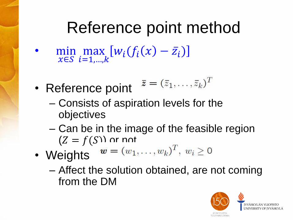
• min𝑥∈𝑆
max𝑖=1,…,𝑘
𝑤𝑖(𝑓𝑖 𝑥 − 𝑧 𝑖)
• Reference point
– Consists of aspiration levels for the objectives
– Can be in the image of the feasible region (𝑍 = 𝑓(𝑆)) or not
• Weights
– Affect the solution obtained, are not coming from the DM
Reference point method

Effect of the weights
f1, min
f2,
min
nadz
1z*z
2z
*1
i
nad
iizzw
*1
iiizzw
i
nad
iizzw
1

Reference point method
Results:
– Reference point method produces weakly PO
solutions
– Every weakly PO solution can be found
– Scalarization of the reference point method can be
changed so that the solution obtained is PO

Reference point method
Scalarized problem is not differentiable due to
the min-max form
Can be reformulated in order to have
differentiable form (if the objective are
differentiable)
– An additional variable and extra constraints
min𝑥∈𝑆,𝛿∈𝑅
𝛿 𝑠. 𝑡. 𝑤𝑖 𝑓𝑖 𝑥 − 𝑧 𝑖 ≤ 𝛿 ∀ 𝑖 = 1,… , 𝑘

Satisficing Trade-Off Method (STOM)
Interactive method, based on classification of
the objective functions
Very similar to the idea of the reference point
method
Nakayama & Sawaragi, “Satisficing Trade-Off
Method for Multiobjective Programming”, In:
Interactive Decision Analysis, Springer-Verlag,
1984

Satisficing Trade-Off Method (STOM)
DM classifies the objectives into 3 classes at the current PO solution – 𝑓𝑖, whose values should be improved
– 𝑓𝑖, whose value is satisfactory at the moment
– 𝑓𝑖 whose value is allowed to get worse
A reference point is formed based on the classification – DM gives aspiration levels for the functions in the first class
– Aspiration levels for the functions in the second class are the current values
– Aspiration levels for the functions in the third class can be computed by using automatic trade-off → help for the DM

Satisficing Trade-Off Method (STOM)
min𝑥∈𝑆
max𝑖=1,…,𝑘
𝑓𝑖 𝑥 −𝑧𝑖∗
𝑧 𝑖−𝑧𝑖∗ + 𝜌
𝑓𝑖(𝑥)
𝑧 𝑖−𝑧𝑖∗
𝑘𝑖=1
Aspiration levels must be greater than the
components of the ideal objective vector
A solution of the scalarized problem in STOM
is PO (if the augmentation term is used)

Satisficing Trade-Off Method (STOM)
f1, min
f2,
min
nadz
1z*z
2z
*1
iiizzw

NIMBUS method
Interactive method, based on classification of the
objectives
Classification: consider the current PO solution
and set every objective into one of the classes
Miettinen, Nonlinear Multiobjective Optimization,
Kluwer Academic Publishers, 1999
Miettinen & Mäkelä, ” Synchronous Approach in
Interactive Multiobjective Optimization”, European
Journal of Operational Research, 170, 2006

NIMBUS method
5 classes consist of objectives 𝑓𝑖 whose values
– should be improved as much as possible (i є Iimp)
– should be improved until 𝑧 𝑖 (i є Iasp)
– is satisfactory at the moment (i є Isat)
– Is allowed to get worse until 𝜖𝑖 (i є Ibound)
– Can change freely at the moment (i є Ifree)

NIMBUS method
Classification is feasible if
A scalarized problem is formed based on the
classification (𝑥𝑐 is the current PO solution)
min𝑥∈𝑆
max𝑖∈𝐼𝑖𝑚𝑝,𝑗∈𝐼𝑎𝑠𝑝
𝑓𝑖 𝑥 −𝑧𝑖∗
𝑧𝑖𝑛𝑎𝑑−𝑧𝑖
∗ ,𝑓𝑗 𝑥 −𝑧 𝑗
𝑧𝑗𝑛𝑎𝑑−𝑧𝑗
∗ + 𝜌 𝑓𝑖(𝑥)
𝑧𝑖𝑛𝑎𝑑−𝑧𝑖
∗𝑘𝑖=1
𝑠. 𝑡. 𝑓𝑖 𝑥 ≤ 𝑓𝑖 𝑥𝑐 ∀ 𝑖 ∈ 𝐼𝑖𝑚𝑝 ∪ 𝐼𝑎𝑠𝑝 ∪ 𝐼𝑠𝑎𝑡,
𝑓𝑖 𝑥 ≤ 𝜖𝑖 ∀ 𝑖 ∈ 𝐼𝑏𝑜𝑢𝑛𝑑

NIMBUS method
Results:
– Solution of the scalarized problem in the NIMBUS
method is weakly PO without the augmentation term
– It is PO if the augmentation term is used
In the synchronous NIMBUS method, 4 different
scalarizations are used
– Different solutions can be obtained for the same
preference information
– No just one way to scalarize the problem, the DM gets
to choose from the solutions obtained

WWW-NIMBUS: implementation of the NIMBUS
method operating on the Internet
1st multiobjective optimization software
operating on the Internet (2000)
All the computations are done in servers at JYU,
only a browser is needed
Always the latest version available
Graphical user interface based on forms
Freely available for academic purposes
http://nimbus.it.jyu.fi/

http://www.mcdmsociety.org/
Newsletter
23rd International Conference on Multiple
Criteria Decision Making
3-7 August 2015, Hamburg (Germany)
Membership does not cost you anything!
January 23-27, 2012 Dagstuhl Seminar on Learning in
Multiobjective Optimization