the winner–loser effect in japanese stock returns

The winner–loser effect in Japanese stock returns

Yoshio Iiharaa, Hideaki Kiyoshi Katob,d,*, Toshifumi Tokunagac

aSchool of Business Administration, Toyo University, Tokyo, JapanbGraduate School of Business Sciences, University of Tsukuba, 3-29-1 Otsuka, Bunkyo-ku,

Tokyo 112-0012, JapancSchool of Business Administration, Nanzan University, Nagoya, JapandGraduate School of Business Sciences, Kobe University, Kobe, Japan

Received 23 April 2002; received in revised form 8 May 2003; accepted 30 June 2003

Abstract

This study examines the winner–loser effect using stocks listed on the Tokyo Stock Exchange

(TSE) from 1975 to 1997. We uncover significant return reversals dominating the Japanese markets,

especially over shorter periods such as 1 month. No momentum effect is observed, however. The 1-

month return reversal remains significant even after adjusting for firm characteristics or risk. While

the 1-month return reversal is not related to industry classification, it is partially a result of higher

future returns to loser stocks with low trading volume. Our results show that investor overreaction

may be a possible explanation for the 1-month return reversal in Japan.

# 2003 Elsevier B.V. All rights reserved.

JEL classification: G10; G12; G14; G15

Keywords: Contrarian; Momentum; Predictability

1. Introduction

One of the striking empirical findings in recent financial research is the evidence of

predictability in asset returns. Many articles in the recent literature find that mean stock

returns are related to past stock price performance. Though accounting-related variables

such as firm size, book-to-market equity, and cash flow to equity ratios are able to capture

the cross-sectional variation in average returns, there is only a weak positive relation

between average returns and beta using the Capital Asset Pricing Model (CAPM).

In their seminal papers, De Bondt and Thaler (1985, 1987) document return reversals

over long horizons ranging from 3 to 5 years. Firms with poor past performance earn

Japan and the World Economy

16 (2004) 471–485

* Corresponding author. Tel.: þ11-81-78-803-6957; fax: þ11-81-78-803-6977.

E-mail address: [email protected] (H.K. Kato).

0922-1425/$ – see front matter # 2003 Elsevier B.V. All rights reserved.

doi:10.1016/j.japwor.2003.06.001

significantly higher returns in the subsequent period than those with above average past

performance. This implies that a contrarian trading strategy performs well. In addition,

winner–loser reversals seem to be related both to firm size and to the seasonal patterns of

returns, especially January returns. Richards (1997) finds similar winner–loser return

reversals in 16 national stock market indices after adjusting for risk.

On the other hand, several papers document that over medium-term horizons ranging

from 6 to 12 months, stock returns exhibit momentum, that is, past winners continue to

perform well and past losers continue to perform poorly in the following period. For

example, Jegadeesh and Titman (1993) find that a strategy that buys past 6-month

winners and shorts past 6-month losers earns approximately 1 percent per month over

the subsequent 6-month period. Rouwenhorst (1998) documents a similar return con-

tinuation in 12 European countries, which suggests that return continuation is a global

phenomenon.

Although there is compelling empirical evidence that both contrarian and momentum

strategies offer superior returns, the extant literature has failed to offer a conclusive

explanation. There are two competing arguments explaining these anomalies with regard to

market efficiency. The proponents of the efficient market view argue that the higher

average returns from these strategies simply represent the reward from investing in risky

stocks, which may not be captured by the CAPM. Fama and French (1993, 1996, 1998)

propose a three-factor model in order to capture the cross-sectional variation in returns.

Except for the continuation of medium-term returns, the anomalous patterns largely

disappear in their three-factor model.

The opponents of the efficient market view take a behavioral approach. The superior

return on these stocks is due to expectation errors made by investors. Investors overreact,

and their excessive optimism or pessimism causes prices to be driven too high above, or too

low below their fundamental values, and that the overreaction is corrected in a subsequent

period. Similarly, investors under-react to information. They do not revise their own

estimates in a timely fashion when they receive new information. As a result, asset prices

do not fully reflect new information.

Daniel et al. (1998a,b) propose a theory of stock market over (or under) reaction based

on two psychological biases—investor overconfidence about the precision of private

information, and biased self-attribution—which causes asymmetric shifts in investor

confidence as a function of their outcomes.1 Investors tend to be overconfident about

their estimates. The theory predicts negative long-lag autocorrelations, excess volatility,

and positive short-lag autocorrelations.

Several studies attempt to investigate how return reversals and return continuation are

related to other factors. For example, Moskowitz and Grinblatt (1999) have recently shown

that a significant component of firm-specific momentum can be explained by industry

momentum. Liew and Vassalou (1999) find that portfolios based upon firm size and book-

to-market contain significant information about future economic growth, however,

momentum-related portfolio returns do not seem to be related to future economic growth.

1 Daniel and Titman (1999) also discuss investor overconfidence and market efficiency. Chan et al. (1996) find

that medium-term return continuation can be explained in part by under-reaction to earnings information, but

price momentum is not subsumed by earnings momentum.

472 Y. Iihara et al. / Japan and the World Economy 16 (2004) 471–485

Several studies have focused on the Japanese stock markets concerning stock return

regularities. Kato (1990) documents a long-term return reversal in which losers out-

perform winners. However, winners do not perform badly in the subsequent period,

unlike US firms. Furthermore, the January effect does not appear in these data. Bremer

and Hiraki (1999) have recently documented a short-term return reversal using Japanese

weekly stock returns. They find that loser stocks with high trading volume in the

previous week tend to have larger return reversals in the following week. Chan et al.

(1991) examine a cross-sectional relationship between portfolio returns and accounting-

related variables such as earnings to price (E/P), firm size (F/S), book-to-market (B/M),

and cash flow to price (C/P). They find that E/P, B/M, and C/P are positively related to

returns, while F/S is a negative determinant. Kobayashi (1997) analyzes the relationship

between B/M and the return reversals and documents that the B/M effect is independent

of return reversals.

In this paper, we conduct a comprehensive analysis of the winner–loser effect using

stocks listed on the Tokyo Stock Exchange (TSE) during the period from 1975 to 1997. Our

major findings are:

1. Return reversals dominate in Japanese stock markets, especially over short horizons

such as 1 month.

2. No momentum effect is observed.

3. The 1-month return reversal is significant even after adjusting for firm characteristics

and risk.

4. The 1-month return reversal is not related to industry classification and is weakly

related to trading volume.

5. Investor overreaction may be the cause of the 1-month return reversal in Japan.

The next section documents anomalous patterns observed in Japanese stock returns by

constructing portfolios based upon past performance. We uncover return reversals dom-

inating Japanese stock markets, especially over short horizons. Our results are different

from US findings, which document return reversals over long horizons ranging from 3 to 5

years. In addition, no momentum effect is observed in Japan though it is significant in many

countries including the US.

In the third section, we investigate whether the Fama–French three-factor model or

the characteristic model is able to explain return reversals in Japan. Our results show that

these two models can explain most of the return reversals but neither model can

successfully capture the 1-month return reversal in Japan. Like the momentum effect

in the US, the 1-month return reversal in Japan may be an additional factor to be

considered.

In the fourth section, we attempt to explain the 1-month return reversal focusing on three

different factors, which are industry classification, trading volume and investor over-

reaction. Though US studies document a relationship between industry classification and

momentum effect, the 1-month return reversal in Japan is independent of industry

classification. Our results regarding trading volume are also different from those of US

studies. The 1-month return reversal is partially caused by higher future returns of loser

stocks with low trading volume. Finally, focusing on each firm’s fiscal year, we show that

the 1-month return reversal is related to investor overreaction.

Y. Iihara et al. / Japan and the World Economy 16 (2004) 471–485 473

2. Do patterns exist in Japan?

Because of the popularity of technical analysis, both contrarian and momentum

strategies have received a lot of attention from Japanese investors in past years. In this

section, we attempt to identify specific patterns in Japanese stock returns using data

covering longer periods with a variety of portfolio formation and holding periods. The data

used in this study are from the database compiled by Pacific Basin Capital Market Research

Center (PACAP) at the University of Rhode Island. This database contains a variety of

information including monthly stock returns and accounting related values covering the

period from 1975 to 1997.2

We form five equally weighted portfolios ranked on past performance following the

approach of Jegadeesh and Titman (1993). The ranking variable used in this study is a

stock’s past compound raw return, extending back 1, 6, 12, 36, and 60 months prior to

portfolio formation (J ¼ 1, 6, 12, 36, 60 months). We also have five holding periods

corresponding to each formation period (K ¼ 1, 6, 12, 36, 60). As a result, we focus on 25

trading strategies with regard to length of formation and holding periods. We do not allow

overlapping of formation periods when the portfolios are constructed.

Panel A of Table 1 reports mean monthly returns for the winner and loser portfolios as

well as the zero-cost contrarian (loser minus winner) portfolio, for the 25 trading strategies.

Significant return reversals are observed for all formation period portfolios. Loser portfolio

returns exceed winner portfolio returns at all horizons. This is different from US studies,

which show that at horizons of less than 1 year, a momentum effect is observed instead of

return reversals.3 Our results show that losers consistently outperform winners for all

horizons. In other words, no momentum effects are observed in Japanese stock returns. In

addition, the magnitude of the formation period returns decreases as the length of the

formation period increases. The magnitude of holding period returns does not seem to

change across all horizons. As a result, return reversals are more pronounced over shorter

periods.

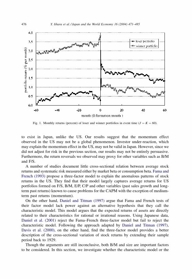
In order to visualize the performance of winner and loser portfolios, we plot the

evolution of the average returns of loser and winner portfolios before and after the time of

formation (J ¼ 60 months) as shown in Fig. 1.4 At the time of formation, average portfolio

returns take a big jump. The average returns of the winner portfolio fall from 3.7 to 1.0

percent. On the other hand, the average returns of the loser portfolio rise from 0.3 to 2.3

percent. Significant return reversals occur for both portfolios.

After the time of formation, average returns of winner and loser portfolios change

dramatically, but in opposite directions. This phenomenon may be attributed to the fact that

more stocks in the winner (loser) portfolio are included in the loser (winner) portfolio in the

following period. We calculate the portions of stocks included in the five ranking portfolios

in the following period. The portions are not evenly distributed across the ranking

portfolios. More stocks in the loser (winner) portfolio are included in the winner (loser)

2 We exclude stocks with negative book equity. Since the PACAP data does not include consolidated financial

statements, we use unconsolidated financial data to compute B/M.3 Richards (1997) and Rouwenhorst (1998) document a similar pattern in the world market.4 We also plot the average returns before and after the formation for the portfolios (J ¼ 1, 6, 12, 36). The

patterns are similar and are not shown here.


portfolio in the following period.5 This implies that winner–loser reversals are not caused

by a few outliers.

In this section, we find strong return reversals in Japanese stock returns across a variety

of formation and holding periods.6 No momentum effect is observed, however. Our results

are consistent with Daniel et al. (1998a) when no self-attribution bias is assumed.

Interestingly, the return reversals are more pronounced for shorter formation periods,

which is different from US findings. In addition, return reversals exist regardless of the

length of holding period.

3. Risk/firm characteristics adjustment

Loser–winner return reversals are clearly observed in Japan for a variety of

formation periods and holding periods. On the other hand, momentum does not seem

Table 1

Mean monthly returns (percent) for winner, loser and contrarian portfolios

J Formation period return Holding period return

K ¼ 1 K ¼ 6 K ¼ 12 K ¼ 36 K ¼ 60

Loser portfolios

1 �8.9788 (�22.05) 1.7843 (3.59) 1.2699 (2.70) 1.1322 (2.47) 1.3815 (2.90) 1.7150 (3.60)

6 �2.7672 (�6.13) 1.7916 (3.40) 1.1951 (2.47) 1.1267 (2.43) 1.4247 (3.02) 1.7526 (3.75)

12 �1.6180 (�3.55) 1.5305 (3.00) 1.1452 (2.40) 1.1456 (2.50) 1.4694 (3.13) 1.7931 (3.83)

36 �0.2883 (�0.60) 1.7095 (3.54) 1.3653 (2.90) 1.3848 (2.99) 1.6627 (3.50) 1.9888 (4.13)

60 0.5674 (1.17) 1.8106 (3.74) 1.4838 (3.11) 1.4641 (3.10) 1.7230 (3.50) 2.0308 (4.02)

Winner portfolios

1 14.0077 (24.43) 0.3898 (0.95) 0.7914 (1.90) 0.9366 (2.18) 1.2320 (2.65) 1.5885 (3.37)

6 6.0117 (12.35) 0.4295 (1.06) 0.8094 (1.86) 0.8963 (2.04) 1.1477 (2.42) 1.5069 (3.15)

12 4.4952 (9.51) 0.5773 (1.41) 0.7883 (1.78) 0.7892 (1.76) 1.0571 (2.19) 1.4239 (2.93)

36 3.1452 (6.64) 0.5154 (1.23) 0.6251 (1.40) 0.6179 (1.36) 0.9151 (1.86) 1.2970 (2.67)

60 3.1554 (6.25) 0.4608 (1.10) 0.5584 (1.26) 0.5894 (1.30) 0.8854 (1.83) 1.2739 (2.68)

Contrarian portfolios

1 �22.9865 (�57.96) 1.3945 (4.70) 0.4786 (3.21) 0.1956 (1.94) 0.1495 (2.17) 0.1265 (1.88)

6 �8.7789 (�29.36) 1.3621 (3.59) 0.3857 (1.38) 0.2304 (1.07) 0.2770 (1.91) 0.2457 (1.89)

12 �6.1132 (�20.67) 0.9532 (2.62) 0.3569 (1.19) 0.3564 (1.37) 0.4123 (2.16) 0.3692 (2.13)

36 �3.4336 (�10.92) 1.1941 (3.65) 0.7402 (2.38) 0.7670 (2.61) 0.7476 (3.25) 0.6918 (2.91)

60 �2.5881 (�8.02) 1.3498 (4.64) 0.9254 (3.32) 0.8747 (3.27) 0.8375 (3.16) 0.7569 (2.70)

Winner and loser portfolios are formed based on J-month lagged returns and held for K-months. The stocks are

ranked in ascending order on the basis of J-month lagged returns. An equally weighted portfolio of stocks in the

lowest past return quintile is the loser portfolio and an equally weighted portfolio of stocks in the highest past return

quintile is the winner portfolio. The contrarian portfolio is a zero investment portfolio, which is long in the loser and

short in the winner. The average returns of these portfolio are presented in this table. t-statistics are in parenthesis.

5 We conduct the same analysis for the J ¼ K ¼ 1 and the J ¼ K ¼ 12 portfolios. The results remain

qualitatively unchanged.6 We also conducted the same analysis by splitting the sample into two periods, the 1980s and the 1990s. We

find that the return reversals are more pronounced during the 1990s.


to exist in Japan, unlike the US. Our results suggest that the momentum effect

observed in the US may not be a global phenomenon. Investor under-reaction, which

may explain the momentum effect in the US, may not be valid in Japan. However, since we

did not adjust for risk in the previous section, our results may not be entirely persuasive.

Furthermore, the return reversals we observed may proxy for other variables such as B/M

and F/S.

A number of studies document little cross-sectional relation between average stock

returns and systematic risk measured either by market beta or consumption beta. Fama and

French (1993) propose a three-factor model to explain the anomalous patterns of stock

returns in the US. They find that their model largely captures average returns for US

portfolios formed on F/S, B/M, E/P, C/P and other variables (past sales growth and long-

term past returns) known to cause problems for the CAPM with the exception of medium-

term past returns (momentum).

On the other hand, Daniel and Titman (1997) argue that Fama and French tests of

their factor model lack power against an alternative hypothesis that they call the

characteristic model. This model argues that the expected returns of assets are directly

related to their characteristics for rational or irrational reasons. Using Japanese data,

Daniel et al. (2001) reject the Fama–French three-factor model but fail to reject the

characteristic model. Following the approach adapted by Daniel and Titman (1997),

Davis et al. (2000), on the other hand, find the three-factor model provides a better

description of the cross-sectional variation of stock returns by extending their sample

period back to 1929.

Though the arguments are still inconclusive, both B/M and size are important factors

to be considered. In this section, we investigate whether the characteristic model or the

Fig. 1. Monthly returns (percent) of loser and winner portfolios in event time (J ¼ K ¼ 60).


three-factor model can explain return reversals in Japan. First, we follow the procedure

used in Daniel et al. (1997) for the characteristic model.

We form a set of 25 benchmark portfolios with similar stock characteristics, B/M and

F/S. At the end of each June from 1975 to 1997, all TSE stocks in the sample are sorted

into five equal groups from small to large based upon their F/S.7 F/S is market

capitalization at the end of June for each year. We also separately sort TSE stocks

into five equal B/M groups from low to high. B/M is equal to the ratio of book value to

market equity at the end of June for each year.8 The 25 portfolios are created from the

Table 2

Excess returns (percent) adjusted by the characteristic model

J K

1 6 12 36 60

Loser portfolios

1 0.6343 (4.64) 0.1238 (1.85) �0.0023 (�0.04) �0.0066 (�0.15) �0.0260 (�0.56)

6 0.4981 (2.90) 0.0204 (0.16) �0.0672 (�0.73) �0.0219 (�0.38) �0.0344 (�0.64)

12 0.1875 (1.19) �0.0990 (�0.78) �0.0906 (�0.85) �0.0301 (�0.44) �0.0429 (�0.72)

36 0.2519 (2.04) 0.0102 (0.09) 0.0302 (0.30) 0.0874 (1.12) 0.0785 (1.04)

60 0.3183 (3.23) 0.1055 (1.14) 0.0967 (1.09) 0.1226 (1.32) 0.1117 (1.16)

Winner portfolios

1 �0.7491 (�5.70) �0.2241 (�3.65) �0.0951 (�2.39) �0.0732 (�2.23) �0.07‘81 (�1.77)

6 �0.5283 (�3.56) �0.0967 (�0.94) �0.0066 (�0.08) �0.0583 (�1.02) �0.0767 (�1.27)

12 �0.3341 (�2.34) �0.0482 (�0.42) �0.0605 (�0.62) �0.1008 (�1.42) �0.1188 (�1.61)

36 �0.3278 (�3.29) �0.1475 (�1.63) �0.1502 (�1.64) �0.1674 (�1.76) �0.1845 (�1.64)

60 �0.3184 (�3.44) �0.1842 (�2.02) �0.1666 (�1.73) �0.1790 (�1.52) �0.1932 (�1.39)

Contrarian portfolios

1 1.3833 (5.50) 0.3479 (2.89) 0.0927 (1.14) 0.0666 (1.34) 0.0520 (1.07)

6 1.0264 (3.34) 0.1171 (0.53) �0.0606 (�0.37) 0.0364 (0.39) 0.0423 (0.52)

12 0.5216 (1.82) �0.0508 (�0.22) �0.0300 (�0.15) 0.0707 (0.59) 0.0759 (0.74)

36 0.5797 (2.76) 0.1577 (0.83) 0.1804 (1.00) 0.2548 (1.65) 0.2630 (1.60)

60 0.6366 (3.67) 0.2897 (1.75) 0.2633 (1.58) 0.3016 (1.59) 0.3050 (1.44)

Winner and loser portfolios are formed based on J-month lagged returns and held for K-months. The stocks are

ranked in ascending order on the basis of J-month lagged returns. An equally weighted portfolio of stocks in the

lowest past return quintile is the loser group and an equally weighted portfolio of stocks in the highest past return

quintile is the winner. The contrarian portfolios are zero investment portfolios that are long in the loser and short

in the winner portfolios. The excess return of a particular stock is computed by subtracting the benchmark

portfolio’s return from the stock’s return. t-statistics are in parenthesis.

7 The majority of Japanese firms have their fiscal year ending in March (more than 80 percent of the firms in

year of 2000), and essentially all companies publish their financial statements within 3 months after the end of

their fiscal year. Accordingly, the portfolios are formed on the basis of the fundamental variables known to

investors as of the end of June for firms with March and non-March fiscal year-ends. This ensures that our tests

are predictive in nature.8 We took both book value of stock and number of shares issued from the balance sheet of the previous fiscal

year. The data available to us are from parent-only financial statements. Though the consolidated financial

statement has become more important over the last few years, parent-only statements had more influence on

stock prices during our sample period.


intersections of the five size and five book-to-market groups. Monthly equal-weighted

returns for each of these 25 portfolios are calculated from June of year t to June of year

t þ 1.

Using these 25 benchmark portfolio returns, we compute excess returns for the

25 past-performance-based trading strategies (J ¼ 1–60 months, K ¼ 1–60), as pre-

sented in Table 2.9 Table 2 shows the performance of winner, loser and contrarian

portfolios after adjusting for the characteristic premium. The characteristic model seems

to explain most of the return reversals in Japan except for the shorter return reversals.

Both winner and loser portfolios exhibit significant return reversals for the 1 month

holding strategy (J ¼ 1–60 months, K ¼ 1). As a result, contrarian portfolios have

significantly positive returns. The 1-month return reversal is larger as the formation

period becomes shorter. Return reversals seem to disappear for longer holding strategies

except the J ¼ 1 month and K ¼ 6 trading strategies. The 1-month return reversal may

be another characteristic to be added to the characteristic model for Japan. This is

somewhat different from the US evidence which finds evidence of a significant medium-

term return continuation.

In order to test the robustness of our results, we apply the procedure used by Fama and

French (1993) for their three-factor model. The following time series regression is

estimated for each of the past-performance-based trading strategies.

Ri;t � Rf;t ¼ ai þ bi;HMLðRHML;tÞ þ bi;SMBðRSMB;tÞ þ bi;MktðRMkt;tÞ þ ei;t (1)

where Ri,t is the return of past-performance-based portfolio i, and RHML,t, RSMB,t,

RMkt,t are respectively, the returns on the HML, SMB and Mkt factor portfolios at

time t. Rf,t is the risk-free rate at time t; bi,j is the factor loading of portfolio i on

factor j. HML is a zero investment portfolio, which is long high B/M stocks and short

low B/M stocks.10 SMB is a zero investment portfolio, which is long small stocks and

short large stocks.11 Mkt is a zero investment portfolio, which is long the market

portfolio and short the risk-free asset. We use the returns of an equally weighted

portfolio of all stocks listed on the Tokyo Stock Exchange as a proxy for the market

portfolio.

Since we have 25 different trading strategies based on past performance, we need to

create time series observations of holding period returns for each strategy (J ¼ 1–60

months and K ¼ 1–60). However, we are not able to obtain a sufficient number of non-

overlapping observations for the longer period trading strategies (K ¼ 36 or 60) because of

the limited length of our sample period. Therefore, we focus on 15 shorter period trading

strategies (J ¼ 1–60 months, K ¼ 1–12). For each trading strategy, we form five portfolios

based upon past performance. When J equals 1, we rebalance the performance-based

9 The excess return of a particular stock is computed by subtracting the benchmark portfolio’s return from the

stock’s return.10 At the end of June of year t, we form three groups using B/M for the fiscal year-end that falls between July

of year t �1 and June of year t. B/M is equal to the ratio of book value to market equity at the end of

June in year t.11 Similarly, we form two groups based upon F/S at the end of each June. F/S is market capitalization at the

end of each June.


portfolios every month. Accordingly, when K equals 6 (or 12), we rebalance the

performance-based portfolios every 6 months (or every year). We estimate a time series

regression for each of the five ranking portfolios for each strategy.

The intercepts and t-statistics of the Fama–French three-factor model are presented in

Table 3.12 The three-factor model seems to capture most of the return reversals in Japan.

Most of the t-statistics are insignificant except for a few winner portfolios (J ¼ 1, 6;

K ¼ 1) and a loser portfolio (J ¼ K ¼ 1). Our results show that the 1-month return

reversal (J ¼ K ¼ 1) remains significant even after adjusting for risk using the three-

factor model.

In this section, we investigated whether the characteristic model and the three-factor

model, successfully explain return reversals in Japan. Most of the long-term return

reversals disappear after adjusting for firm characteristic or risk. However, the short-term

Table 3

Tests for alpha of Fama–French three-factor regressions

J Rank 1 (loser) Rank 2 Rank 3 Rank 4 Rank 5 (winner)

Holding period (K ¼ 1)

1 0.3900 (1.88) 0.0077 (0.05) �0.1101 (�0.96) �0.2831 (�2.24) �0.7326 (�4.18)

6 0.2094 (0.84) �0.0128 (�0.09) �0.2472 (�2.15) �0.2588 (�1.93) �0.4043 (�2.13)

12 �0.2239 (�0.95) �0.1785 (�1.28) �0.1453 (�1.27) �0.0664 (�0.49) �0.0873 (�0.54)

36 �0.2462 (�1.40) �0.1019 (�0.77) �0.0336 (�0.27) �0.1644 (�1.30) �0.0903 (�0.70)

60 �0.0665 (�0.45) �0.1024 (�0.77) �0.1186 (�0.94) �0.1609 (�1.26) �0.1684 (�1.29)

Holding period (K ¼ 6)

1 3.0259 (1.00) 2.1832 (0.83) 1.2773 (0.52) 0.7542 (0.33) �0.8726 (�0.29)

6 3.5457 (1.11) 2.6576 (0.89) 1.6602 (0.66) 0.4274 (0.17) �1.8222 (�0.82)

12 2.5468 (0.81) 2.7954 (0.95) 2.2607 (0.85) 0.9001 (0.34) �1.9534 (�1.03)

36 2.9521 (0.86) 2.7799 (0.91) 2.2900 (0.83) 0.3773 (0.12) �1.7808 (�1.04)

60 4.2064 (1.18) 2.9113 (0.89) 1.7680 (0.69) 0.1424 (0.02) �2.5476 (�1.43)

Holding Period (K ¼ 12)

1 �0.9802 (�0.12) �3.4364 (�0.49) �4.3448 (�0.61) �4.1756 (�0.55) �3.6471 (�0.62)

6 �1.5401 (�0.13) �3.2451 (�0.39) �3.5423 (�0.53) �3.8418 (�0.61) �4.5366 (�0.76)

12 �2.4713 (�0.27) �3.5075 (�0.43) �3.6122 (�0.52) �3.5514 (�0.57) �3.5393 (�0.75)

36 �1.7609 (�0.15) �2.1038 (�0.23) �3.2134 (�0.43) �5.3710 (�0.99) �4.7516 (�0.93)

60 �0.4958 (�0.03) �3.1191 (�0.34) �3.3690 (�0.48) �5.1701 (�0.99) �5.2302 (�1.07)

Ri;t � Rf ;t ¼ ai þ bi;HMLðRHML;tÞ þ bi;SMBðRSMB;tÞ þ bi;MktðRMkt;tÞ þ ei;t

Ri,t is the monthly return of past-performance-based portfolio i in month t. Rf,t is the 1 month risk-free rate. RMkt,t is

the monthly return of a zero investment portfolio, which is long the market portfolio and short the risk free asset.

RHML,t is the monthly return of a zero investment portfolio, which is long high B/M stocks and short low B/M

stocks. RSMB,t is the monthly return of a zero investment portfolio, which is long small stocks and short large

stocks. t-statistics are reported in parentheses.

12 For comparison purposes, we also consider a one-factor model (CAPM). Most of the t-statistics are

significant for the K ¼ 1 trading strategy, suggesting that the CAPM does not explain return reversals for a

shorter holding period. However, the CAPM successfully explains return reversals for a longer holding period.

This is similar to the results for the characteristic model in the previous section.


return reversals, especially for the J ¼ K ¼ 1 (1-month) trading strategy remain signifi-

cant. We analyze this anomaly in more detail in the following section.

4. Further analysis

Most return reversals diminish after adjusting for risk or firm characteristics. However,

neither the three-factor model nor the characteristic model (B/M and F/S) can successfully

explain the 1-month return reversal (J ¼ K ¼ 1) in Japan. The 1-month return reversal can

be considered risk or characteristic specific to Japan, similar to the momentum phenom-

enon in the US. In this section, we further examine this anomaly focusing on industry

classification, trading volume and investor overreaction. We use excess returns adjusted by

the characteristic model for the analysis in this section.

4.1. Industry classification

Moskowitz and Grinblatt (1999) document a strong and prevalent momentum effect in

industry components of stock returns that accounts for much of the individual stock

momentum anomaly. Though momentum does not exist in Japan, the 1-month return

reversal may be related to industrial classification. In order to examine this possibility, we

sort 33 Tokyo Stock Exchange industry indices into five groups based upon past stock

performance using the previous month’s industry index returns. Each group contains six or

seven industries. For each group, we compute an equally weighted return for each

industry’s index. We do not observe any particular patterns in stock returns after the

formation period, however. Winners do not necessarily become losers (or winners) and

losers do not become winners (or losers). We conclude that industry-based contrarian (or

momentum) portfolios do not show superior performance. Although industry momentum

exists in the US, we do not observe such patterns in Japan. In addition, we find no return

reversals in industry-based portfolios.

Next, we examine the intra-industry effect. The 1-month return reversal may exist only

in particular industries. In order to test this conjecture, we classify firms into three groups,

manufacturers, financial firms and others. In each group, we conduct the same analysis as

in the previous section by forming five performance-based portfolios every month

(J ¼ K ¼ 1). One-month loser, winner and contrarian portfolios are created to examine

excess returns in both the formation and the holding months. The results are presented in

Table 4. Significant return reversals are observed for both winner and loser portfolios

across all three industries. The contrarian portfolio returns are significantly positive across

all three industries as well. Our analysis shows that the 1-month return reversal is not

related to industry classification.

4.2. Trading volume

Trading volume may be a proxy for the amount of information received by the market.

Low trading volume may indicate that less information about a firm is available to

investors. Because of limited information and low liquidity, a majority of investors,


especially institutional investors, may stay away from these low trading volume stocks.

These stocks are sometimes called neglected stocks. These neglected stocks are likely to be

candidates for investor under or overreaction to new information. In other words, these

stocks may be mispriced from time to time.

Conrad et al. (1994) show that return reversals are observed only for heavily traded

stocks; less traded stocks exhibit return continuation. Lee and Swaminathan (2000) show

that past trading volume provides an important link between momentum and value

strategies. Firms with high (low) past turnover ratios exhibit many glamour (value)

characteristics and earn lower (higher) future returns. In a related study, Brennan et al.

(1998) use dollar trading volume as a proxy of liquidity and find low liquidity stocks earn

higher returns than high liquidity stocks. Their results are consistent with the liquidity

hypothesis.13 Using Japanese weekly stock returns data, Bremer and Hiraki (1999) find that

loser stocks with high trading volume in the previous week tend to have larger return

reversals in the following week.

We examine the interaction between past returns and past trading volume in predicting

future returns over a 1-month period. We use monthly turnover as a measure of trading

volume.14 We split the sample into three groups based upon trading volume and form five

performance-based portfolios for each group. The results are presented in Table 5. The

relationship between trading volume and the 1-month return reversal is not strong. The

loser–winner reversal is more pronounced among low trading volume stocks, which is

opposite to the result of Conrad et al. (1994). This is mainly caused by the higher

future returns of low trading volume loser stocks. Our finding is different from that

of Lee and Swaminathan (2000), which document higher future returns for both loser and

Table 4

Excess returns (percent) for performance-based portfolios (J ¼ K ¼ 1) by industry classification

Formation period (J ¼ 1) Holding period (K ¼ 1)

Manufacturer Finance Other Manufacturer Finance Other

Loser �9.0148

(�21.12)

�6.3149

(�14.68)

�8.8495

(�21.17)

0.6163

(3.82)

0.6147

(2.20)

0.7751

(4.70)

Winner 14.2068

(24.60)

9.9341

(13.99)

13.6678

(21.24)

�0.7872

(�5.58)

�0.2802

(�0.80)

�1.0469

(�5.19)

Contrarian �23.2215

(�61.91)

�16.2490

(�26.23)

�22.5173

(�46.72)

1.4035

(5.41)

0.8949

(2.74)

1.8221

(6.96)

In each month t, all stocks listed on the Tokyo Stock Exchange (TSE) are sorted into three groups

(manufacturers, finance, or other) based on industrial classification. The stocks in the manufacturer, finance, and

other groups are ranked in ascending order on the basis of 1 month lagged excess returns. An equally weighted

portfolio of the stocks in the highest excess return quintile is defined to be the winner portfolio and an equally

weighted portfolio of the stocks in the lowest excess return quintile is defined to be the loser portfolio. The

contrarian portfolio is a zero investment portfolio, which is long the loser and short the winner portfolios. Excess

returns are computed using the F/S and B/M benchmark portfolios. t-statistics are in parenthesis.

13 According to the liquidity hypothesis, firms with relatively low trading volume are less liquid, and

therefore, command a higher expected return.14 Turnover is defined as the ratio of the number of shares traded to the number of shares issued.


winner stocks with high trading volume. Since low trading volume stocks do not always

earn higher future returns, our results are inconsistent with the liquidity hypothesis. In

addition, our results are somewhat different from Bremer and Hiraki (1999), which use

weekly data.

Our results indicate that the 1-month return reversal is partially caused by the higher future

returns of loser stocks with low trading volume. Low trading volume stocks tend to be

neglected stocks which are candidates for investor overreaction. However, winner stocks

with low trading volume do not have a similar pattern to loser stocks. In the following

section, we examine investor overreaction in more detail by focusing on the turn of the fiscal

year.

4.3. Overreaction to new information

In the previous section, we document the relationship between trading volume and the

1-month return reversal. Japanese investors may overreact to news and as a result,

stock prices may overshoot temporarily and later come back to their fundamental values.

In order to examine investor overreaction over the 1-month period, we focus on the fiscal

year-end month because a large amount of information is released to the market at this

time. For example, under the disclosure rules of the Tokyo Stock Exchange, Japanese firms

must announce revisions to their financial forecasts if their actual audited results are likely

to differ greatly from what they expected.15 This kind of announcement is likely to take

place toward the fiscal year-end because such accounting numbers become available

Table 5

Excess returns (percent) for performance-based portfolios (J ¼ K ¼ 1) by trading volume

Formation period (J ¼ 1) Holding period (K ¼ 1)

Low Medium High Low Medium High

Loser �8.4954

(�23.58)

�8.7375

(�20.85)

�9.0663

(�18.54)

0.7571

(5.94)

0.7735

(4.56)

0.3104

(1.58)

Winner 9.0808

(19.36)

9.4236

(18.37)

20.5575

(28.06)

�0.6631

(�3.34)

�0.5303

(�4.23)

�0.8742

(�4.81)

Contrarian �17.5762

(�46.44)

�18.1611

(�56.02)

�29.6238

(�57.22)

1.4202

(5.55)

1.3038

(5.23)

1.1846

(3.99)

In each month t, all stocks listed on the Tokyo Stock Exchange (TSE) are sorted into three groups based on

trading volume (turnover ratio). The stocks in the low, medium and high volume groups are ranked in ascending

order on the basis of 1 month lagged excess returns. An equally weighted portfolio of the stocks in the highest

excess return quintile is defined as the winner portfolio and an equally weighted portfolio of the stocks in the

lowest excess return quintile is defined as the loser portfolio. The contrarian portfolio is a zero investment

portfolio, which is long the loser and short the winner portfolios. The excess returns are computed using the F/S

and B/M benchmark portfolios. t-statistics are in parenthesis.

15 When actual sales differ by more than 10 percent from the forecast, the firm must announce revisions.

When actual operating income or actual net profit differs by more than 30 percent from the forecasts, the firm

must announce revisions. When the actual dividend differs more by than 20 percent from the forecast, the firm

must also announce the revision.


at this time. Top management changes are also likely to occur during this period as a result;

a change of corporate strategy may also be announced. Security analysts respond to the

above information, revise their forecasts and release new forecasts toward the firm’s fiscal

year-end.

Since a majority of Japanese firms set their fiscal year-end in March, the performance

of these stocks in March and April is worth examining.16 If investors overreact to the

new information, the bad (good) news firms are likely to be undervalued (overvalued) at

the fiscal year-end month. We conduct our analysis focusing on the J ¼ K ¼ 1 trading

strategy.

In order to test this conjecture, the stocks included in the winner (loser) portfolio are

sorted into two groups based upon the firm’s fiscal year-end: March fiscal year-end winner

(loser) firms and non-March fiscal year-end winner (loser) firms. According to the

conjecture, return reversals occur in April for the March fiscal year-end firms. The

March fiscal year-end loser (winner) firms should experience higher (lower) returns in

April than the non-March fiscal year-end loser (winner) firms. As a result, April contrarian

portfolio returns using the March fiscal year-end winner and loser firms should be

significantly positive and larger than those using non-March fiscal year-end winner and

loser firms.17

The results are presented in Table 6. As predicted, April winner returns of March fiscal

year-end firms are significantly negative and lower than those of non-March fiscal year-end

firms. In addition, April contrarian portfolio returns of the March fiscal year-end firms are

significantly positive. April contrarian portfolio returns of March fiscal year-end firms are

higher than those of non-March fiscal year-end firms although the difference is not

statistically significant. However, April loser returns of March fiscal year-end firms do

Table 6

April excess returns (percent) for performance-based portfolios (J ¼ K ¼ 1) by fiscal year-end

Fiscal year-end April excess returns H0

March Non-March

Loser 0.5407 (1.10) 1.1611 (2.29) (�0.88)

Winner �1.3697 (�3.21) 0.5363 (1.06) (�2.88)

Contrarian 1.9103 (2.27) 0.6249 (0.78) (1.11)

Stocks are ranked in ascending order on the basis of 1 month returns at the end of March. The stocks included

in winner (loser) portfolio are divided into two groups based on the company’s fiscal year-end: March and

non-March. An equally weighted winner (loser) portfolio is created for each group. The contrarian portfolio

for each group is created by buying the loser and selling the winner. t-statistics are in parenthesis. t-statistics

test whether the difference between April mean excess returns for March and non-March fiscal year-end firms

equal zero.

16 More than 80 percent of the firms listed on the Tokyo Stock Exchange ended their fiscal year in March,

2000.17 Since the 1-month return reversal is more pronounced for low trading volume stocks, investor overreaction

may also be related to trading volume. In order to test this conjecture, we separate our sample into two groups,

high trading volume stocks and low trading volume stocks and conduct the same analysis. We did not observe

any significant differences between low and high trading volume stock groups.


not earn significantly higher returns than non-March fiscal year-end firms. Our results

weakly support the conjecture that the 1-month return reversal is caused by investor

overreaction around the turn of the fiscal year.

5. Conclusions

This study examines the predictability of Japanese stock returns focusing on past-

performance-based trading strategies. Though stock returns exhibit momentum over short/

medium-term horizons in the US, no such patterns are observed in Japan. Instead, return

reversals are observed, especially for short-term portfolio formation strategies. The 1-month

return reversal remains significant even after adjusting for risk or firm characteristics. Our

results are different from US findings, which show short/medium-term momentum and long-

term return reversals.

We further analyze the 1-month return reversal focusing on three factors, industry

classification, trading volume and investor overreaction. Though the industry effect is

related to momentum in the US, the 1-month return reversal in Japan is independent of

industry classification. Trading volume is weakly related to the 1-month return reversal.

Our results show that the 1-month return reversal is partially a result of higher future

returns of loser stocks with low trading volume. This may be consistent with investor

overreaction. Low trading volume stocks tend to be neglected stocks because less

information is available to the investors about these securities. Investors are more likely

to overreact to new information on these stocks.

We further examine investor overreaction focusing on stock returns around the turn of

the fiscal year. Towards the end of the fiscal year, a variety of information is released to the

market. If investors overreact to new information, stock prices are likely to be mispriced at

the fiscal year-end month. We split the sample into March fiscal year-end firms and non-

March fiscal year-end firms to examine this conjecture. Our results show that the 1-month

return reversal is related to investor overreaction.

Overall, we find no return continuations but return reversals in Japan. Specifically, low

trading volume losers in the previous month earn significantly higher returns in the

subsequent month. Our results imply that the 1-month contrarian trading strategy con-

centrating on low trading volume stocks may be effective assuming that this pattern persists

in the future. In addition, a 1-month contrarian portfolio using March fiscal year-end firms

formed at the end of March may earn higher returns in April.

Acknowledgements

We would like to thank Marc Bremer and the participants at the 2002 Korean Finance

Association meeting and the 2002 Pacific Basin Finance Conference/Asian Pacific Finance

Association meeting for their helpful comments. We are also very grateful to the editor,

Ryuzo Sato and an anonymous referee for their insightful comments, which improved the

paper. All remaining errors are our own. Kato thanks JSPS KAKENHI (13303009) for the

financial support.


References

Brennan, M., Chorda, T., Subrahmanyam, A., 1998. Alternative factor specifications, security characteristics,

and the cross-section of expected stock returns. Journal of Financial Economics 49, 345–373.

Bremer, M., Hiraki, T., 1999. Volume and individual security returns on the Tokyo Stock Exchange. Pacific

Basin Finance Journal 7, 351–370.

Chan, L., Hamao, Y., Lakonishok, J., 1991. Fundamentals and stock returns in Japan. Journal of Finance 46,

1739–1789.

Chan, L., Jegadeesh, N., Lakonishok, J., 1996. Momentum strategies. Journal of Finance 51, 1681–1713.

Conrad, J., Hameed, A., Niden, C., 1994. Volume and autocovariances in short-horizon individual security

returns. Journal of Finance 49, 1305–1330.

Daniel, K., Grinblatt, M., Titman, S., Wermers, R., 1997. Measuring mutual fund performance with

characteristic-based benchmarks. Journal of Finance 52, 1035–1058.

Daniel, K., Hirshleifer, D., Subrahmanyam, A., 1998a. Investor psychology and security market under and

overreactions. Journal of Finance 53, 1839–1885.

Daniel, K.,D. Hirshleifer, A., Subrahmanyam, 1998b. Investor overconfidence, covariance risk, and predictors of

securities returns, unpublished manuscript.

Daniel, K., Titman, S., 1997. Evidence on the characteristics of cross-sectional variation in stock returns. Journal

of Finance 52, 1–33.

Daniel, K., Titman, S., 1999. Market efficiency in an irrational world. Financial Analysts Journal 55, 28–40.

Daniel, K., Titman, S., Wei, K.C.J., 2001. Explaining the cross-section of stock returns in Japan: factors or

characteristics? Journal of Finance 56, 743–766.

Davis, J., Fama, E., French, K., 2000. Characteristics, covariances, and average returns 1929–1997. Journal of

Finance 55, 389–406.

De Bondt, W., Thaler, R., 1985. Does the stock market overreact? Journal of Finance 40, 793–805.

De Bondt, W., Thaler, R., 1987. Further evidence on investor overreaction and stock market seasonality. Journal

of Finance 42, 793–805.

Fama, E., French, K., 1993. Common risk factors in the returns on stocks and bonds. Journal of Financial

Economics 33, 3–56.

Fama, E., French, K., 1996. Multifactor explanations of asset pricing anomalies. Journal of Finance 51, 55–84.

Fama, E., French, K., 1998. Value versus growth: the international evidence. Journal of Finance 53, 1975–2000.

Jegadeesh, N., Titman, S., 1993. Returns to buying winners and selling losers: implications for stock market

efficiency. Journal of Finance 48, 65–91.

Kato, K., 1990. Being a winner in the Tokyo Stock Market: the case for an anomaly fund. Journal of Portfolio

Management 16, 52–56.

Kobayashi, T., 1997. Theoretical foundation of style management. Security Analysts Journal, 31–63 (in

Japanese).

Lee, C., Swaminathan, B., 2000. Price momentum and trading volume. Journal of Finance 55, 2017–2069.

Liew, J., Vassalou, M., 1999. Can book-to-market, size and momentum be risk factors that predict economic

growth? Columbia University working paper.

Moskowitz, T., Grinblatt, M., 1999. Do industries explain momentum? Journal of Finance 54, 1249–1290.

Richards, A., 1997. Winner–loser reversals in national stock market indices: can they be explained? Journal of

Finance 52, 2129–2144.

Rouwenhorst, K.G., 1998. International momentum strategies. Journal of Finance 53, 267–284.


the winner–loser effect in japanese stock returns

Documents