the triple-parity law - research repositorythe triple-parity law ... the relative purchasing power...

THE TRIPLE-PARITY LAW

Jean-Christian Lambelet Alexander Mihailov University of Lausanne University of Essex

November 2005

Abstract: Scientists and epistemologists generally agree that a scientific law must be (a) rela-tively simple and (b) not contradicted by the available evidence. In this paper we propose and test one such law pertaining to international economics, the triple-parity law. It integrates three well-known equilibrium conditions, which are shown to prevail in the long run, on aver-age and ex post: (i) uncovered nominal interest rate parity (UIP); (ii) relative purchasing power parity (PPP); (iii) real interest rate parity (RIP). Using a cross-section of annual mean values or trend growth rates for 18 OECD countries in the post-Bretton-Woods/pre-EMU floating rate period (1976-1998) and employing a variety of single-equation and system esti-mation methods, we present robust evidence that the triple-parity law ultimately holds for large and diversified economies. For a few, mostly small and specialized countries, its work-ing is however affected by some significant financial or real comparative (dis)advantages, for which estimates are provided. The law says nothing about short-term dynamics, but it can provide useful benchmarks in this context too, insofar as measures of the speed of conver-gence to long-run equilibrium are estimated. The triple-parity law, finally, illustrates another, rather fundamental point: if we look beyond short-term fluctuations and vagaries, economic laws do exist in the long run, just as economists used to think in the days of Marshall, Fisher, Walras and Pareto.

JEL Classification: C21, C31, E44, F41.

Key words and phrases: nominal interest rate parity, purchasing power parity, real interest rate parity, international arbitrage, economic laws, OECD countries.

___________________________

Acknowledgements: The present paper is a revised version of Lambelet and Mihailov (2001), itself building upon Lambelet (1996). For helpful comments on these previous drafts, special thanks are due Robert Aliber, Philippe Bacchetta, Luca Bindelli, Peter Buomberger, Menzie Chinn, Jean-Pierre Dan-thine, Rumen Dobrinsky, Milton Friedman, Lucien Gardiol, Hans Genberg, Alberto Holly, Jacques Huguenin, Ulrich Kohli, Damian Kozamernik, Vincent Labhard, Jacques L’Huillier, Jean-Marc Natal, Délia Nilles, Michel Peytrignet, Martino Rossi, Jean-Pierre Roth, Claudio Sfreddo, Erich Spörndli, Cédric Tille and Nils Tuchschmid. The usual disclaimer applies.

Jean-Christian Lambelet, DEEP/HEC, University of Lausanne, BFSH1, CH-1015 Lausanne, Switzer-land, 41 (0)21 692 34 81 (tel), 41 (0)21 692 33 55/65 (fax), [email protected], http://www.hec.unil.ch/jlambelet/;

Alexander Mihailov, Department of Economics, University of Essex, Wivenhoe Park, Colchester CO4 3SQ, 44 (0)1206 87 33 51 (tel), 44 (0)1206 87 27 24 (fax), [email protected], http://www.essex.ac.uk/economics/people/staff/mihailov.shtm.

2

Contents

I. Introduction 4

II. Analytical Framework 6

III. Empirical Implementation 9

1. Data: Sources, Definitions and Transformations 9

2. Single-Equation Estimation Methods: OLS, WLS and ODR Results 11

3. The Country-Specific Intercepts: Interpretation as Comparative (Dis)Advantages 19

4. System Estimation Methods: SUR and FIML Results 27

5. Is RIP Independent of UIP and PPP in the “Long Run”? Econometric Tests 31

6. How Long is the “Long Run”? Speed of Convergence to the Triple-Parity Law 33

IV. The Triple-Parity Law and the Closely Related Literature 35

V. Conclusions 37

Appendix A: Data Sources, Definitions and Transformations 40

Appendix B: Direct and Reverse Regression Correspondences and Computations 43

Appendix C: Summary of the Literature on PPP, UIP and RIP as Separate Conditions 46

1. Law of One Price and Purchasing Power Parity: Absolute and Relative Versions 46

2. Nominal Interest Rate Parity: Covered and Uncovered Versions 48

3. Real Interest Rate Parity 50

References 52

List of Tables

1. Triple Parity: Some Illustrative Examples 9

2. First Parity: The Uncovered Nominal Interest Rate Condition 13

3. Second Parity: The Relative PPP Condition 14

3

4. Third Parity: The Real Interest Rate Condition 16

5. Nominal UIP: The “F”-Differentials, or Financial/Institutional Disadvantages 21

6. Correlation Matrix for the Alternative UIP “F”-Differential Estimates (in Table 5) 21

7. Relative PPP: The “R”-Differentials, or Real/Structural Advantages 23

8. RIP: The Combined “F” and “R” Differentials, Overall Disadvantages or RIR Premia 24

9. RIR Discounts: Comparing Indirect (UIP + PPP Implied) and Direct (RIP) Estimates 25

10. Triple Parity: SUR/FIML Pairwise Results 30

11. Triple Parity: Full System SUR vs OLS Results 31

12. RIP Residuals: Comparing Direct (RIP) and Indirect (UIP + PPP Implied) Estimates 32

A1. Nominal Bilateral Exchange Rates Against the US Dollar, annual averages, IFS line rh 40

A2. Long-Run Nominal Interest Rates (Government Bond Yields), in % p.a., IFS line 61 40

A3. Consumer Price Indexes, 1990=100, IFS line 64 41

A4. GDP Deflator Indexes, 1995=100, IFS line 99bip 41

A5. 23-Year (1976-1998) Annual Averages for the Cross-Section of 18 OECD Economies Used in the Triple-Parity Law Tests, USA as Country of Reference 42

List of Figures

1. Uncovered Nominal Interest Parity 13

2. GDP Deflator-Based Purchasing Power Parity 15

3. CPI-Based Purchasing Power Parity 15

4. GDP Deflator-Based Real Interest Parity 17

5. CPI-Based Real Interest Parity 17

6. 1976-1998 Average Real Long-Term Interest Rates Using GDP Deflators 18

7. 1976-1998 Average Nominal Long-Term Interest Rates 19

8. Long-Term Real Interest Rates in Switzerland vs Denmark and Finland 26

9. “Long-Run” Cumulative 95% Confidence Intervals for the Triple-Parity Law 34

4

“Human actions exhibit certain uniformities, and it is solely because of this property that they can be studied scientifically. These uniformities have another name; they are called laws.”

Vilfredo Pareto1

I. Introduction

Scientists and epistemologists tend to agree that, to be worthy of the name, a scientific law must be (a) general enough but relatively simple, and (b) fully consistent, in Popper’s sense (1959), with the available evidence.2 In this paper we propose and test one such law pertain-ing to international economics and applicable to open market economies. We call it the triple-parity law. It integrates three well-known equilibrium conditions, which are shown to prevail in the long run, on average and ex post: (i) the uncovered nominal interest rate parity (UIP) condition, possibly subject to broadly interpreted cross-country financial/institutional premia; (ii) the relative purchasing power parity (PPP) condition, possibly allowing for broadly under-stood cross-country real/structural differentials; (iii) the real interest rate parity (RIP) condi-tion, possibly incorporating country-specific differences of both a financial and a real nature. The triple-parity law thus highlights the interdependence between UIP obtaining from arbi-trage in asset markets and PPP obtaining from arbitrage in goods markets, which ultimately results in a tendency towards equalization of real interest rates.

We employ a simple analytical framework and a number of straightforward yet complemen-tary econometric techniques, to achieve robustness. With few exceptions – such as reverse regression and orthogonal distance regression (ODR), appropriate when estimating arbitrage conditions – these methods are standard. Yet our contribution may be in their original applica-tion and interpretation as well as in a number of novel findings. Our paper is also among the few to view and test RIP as resulting – theoretically but also empirically – from the combina-tion of UIP and PPP. Rather than keeping to the mainstream by resorting to high-frequency time series techniques (with all their well-known imperfections and attendant controversies), or spanning an ultra long period of a century or two (at the cost of working with just a few comparable historical data sequences), we take the stand that economic laws tend to prevail in a “usual” or “standard” long run (up to something like a generation). We therefore purpose-fully isolate our data from both short-term vagaries and too narrow a sampling basis by rely-ing on a cross-section of annual mean values or trend growth rates for 18 OECD countries in the post-Bretton-Woods/pre-EMU floating rate period (1976-1998). We then apply single-equation as well as system estimation methods to confront the theoretical propositions we are interested in with the statistical facts. To our knowledge, such an econometric strategy has not been pursued till now, in particular to formulate and test the joint determination of long-run equilibria in open market economies as embodied in the emergence of RIP out of the interac-tion of UIP and PPP.

The originality of our analytical and empirical approach to these classic and well-explored equilibrium conditions may lie in the following methodological features.

(1) Most papers so far have focused on an individual international arbitrage condition – be it UIP, PPP or RIP – and on a small number of large countries taken two at a time. We use a sample of 18 industrialized countries and check – separately as well as jointly – the three ba-sic conditions across all countries. In essence, we consider and test UIP, PPP and RIP as a 1 Manuel d’économie politique (1966/1909, 5); emphasis in original; our translation (“regularities” might how-ever be a better translation of uniformités than “uniformities”). 2 Blaug (1992, 15) characterizes the (post-)Popperian view of science as an “endless attempt to falsify existing hypotheses and to replace them by ones that successfully resist falsification”.

5

system of long-run equilibrium relations. Yet the issue as to whether RIP can be considered as a separate condition “in its own right” is analyzed too.

(2) The issue of the choice of a country of reference is faced squarely. This question is com-monly ignored, the USA being almost always selected. Our empirical tests of the triple-parity law thus involve a “shifting” cross-section of mean values or growth rate differentials whereby each economy in the sample successively plays the role of the reference country. This enables us to come up with an interpretation of the estimated intercepts in the various regressions as measuring certain comparative (dis)advantage(s) pertaining to each country.

(3) Our econometric strategy, namely to exploit a cross-section of differentials in trend rates of change or mean values over a 23-year period, aims at estimating long-run equilibrium con-ditions directly, filtering out what is likely to include a lot of high-frequency noise and also avoiding a too narrow sample hazard. Doing so, we sidestep a number of pitfalls linked to the usual approaches in the literature – e.g. the danger of overdifferencing, the low power of unit root tests, the difficulty of measuring country specificities in panel data approaches, the somewhat arbitrary judgment of the researcher commonly involved in regime-switching tech-niques and cointegration analyses.

(4) When the equations are initially estimated by single-equation methods, the issue of nor-malization/direction-of-causality as well as the error-in-data problem are addressed explicitly. Regarding the normalization issue, standard errors, t-statistics and confidence intervals from the reverse regressions are transformed so as to be comparable with those from the direct re-gressions.

(5) Single-equation estimation is not confined to ordinary least squares (OLS) or weighted least squares (WLS), but the little-used orthogonal distance regression (ODR) method is em-ployed too. When system estimation methods are applied subsequently, a number of intrigu-ing questions arise, which have not been examined and discussed so far.

Key findings can be summarized as follows.

(1) Our econometric results provide powerful evidence that the triple-parity law holds in the long run, on average and ex post. They therefore confirm – after decades of nihilistic pessi-mism – the direction taken by recent research to the effect that reversal to the mean does oc-cur, eventually and when appropriately measured. Moreover, system estimation methods af-ford even stronger evidence in favor of the triple-parity law than single-equation ones.

(2) The study gives proper attention to the meaning of the nonzero intercepts in the three equations comprising the law, which are interpreted as average country-specific characteris-tics over the sample period. The intercept in the UIP equation is thus interpreted not just as a relative risk premium, as is done in almost all the literature, but more broadly as a finan-cial/institutional premium (or comparative disadvantage). Analogously, the intercept in the PPP equation is interpreted not just as a Balassa-Samuelson effect or productivity differential, as is the case in the earlier literature, but more broadly as a real/structural differential (or comparative advantage). Because of the interdependence we highlight in the triple-parity law, these intercepts then combine into a country-specific overall real interest rate premium (or comparative disadvantage) in the RIP equation.

(3) Numerical estimates of these comparative (dis)advantages are offered for all 18 countries and tested as to their statistical significance. The conclusion is that there are strong indications

6

that financial/institutional premia do exist, but for a small number of small countries only. In the triple-parity law sense, such cases may be considered as anomalies. Indications for real/structural differentials are found for a small number of countries too, but now they in-clude some larger economies (and have less straightforward causes). An attempt is neverthe-less made to explain these findings in terms of specific country characteristics.

(4) We conclude that RIP essentially results from UIP and PPP: the joint validity of UIP and PPP implies RIP, so real interest parity does not seem to be an independent condition in itself. Firstly, its deterministic parts can of course be analytically derived from UIP and PPP. Sec-ondly, although it may tentatively be considered as a separate condition from an econometric standpoint, our tests show that the error term in the RIP regressions is just a combination of the error terms in the UIP and PPP regressions, with a very small margin of imprecision fal-ling well within the 95% confidence interval for the RIP residual variance.

(5) Finally, we provide estimates on how long the “long run” is, i.e. we present computations of the speed of convergence to UIP, PPP and RIP. While UIP holds, on average and ex post, even for a “medium term” of about 5 years, it takes – roughly – twice longer for PPP and thrice longer for RIP to emerge. This means that RIP is jointly determined by UIP and PPP in the very long run, i.e. it takes time for the triple-parity law to prevail as a complete system, and that time is estimated to be of the order of 15-20 years.

The paper is organized as follows. The underlying basic theory is summarized in section II, with only a few references to the literature; the same goes for the empirical results in section III. How our analytical approach, econometric implementation and principal findings relate to those in the existing literature is discussed in section IV. Our conclusions are set forth in sec-tion V. Three appendixes provide more details: Appendix A presents the raw data, their sources and definitions, and the mean differentials into which they were transformed for our purposes; Appendix B summarizes the relation within each pair of direct and reverse simple regressions we use to test UIP, PPP and RIP individually as well as the corresponding calcula-tion and comparison of estimated coefficients and standard errors involving the delta method; Appendix C provides a condensed survey of both the classical and more recent literature on each of the three equilibrium conditions taken separately.

II. Analytical Framework

Consider a two-country world (A and B) where there exists “sufficient” – i.e. not necessarily perfect – mobility of capital, goods and services across the border. Because of capital mobility in asset (or financial) markets, the following first arbitrage condition must hold – and will be shown to hold – in the long run, on average and ex post:

DA/B = (FA – FB) + (IB A – IBB) + e1. (1)

All variables are expressed as trend growth rates (in % p.a.). DA/B is the depreciation rate of currency A with respect to currency B as measured by the spot exchange rate.3 IA and IB are long-term interest rates; their exact definition and measurement will be discussed in section III.1. Of course, e

B

1 is a disturbance term, due to a shock process affecting (1).

3 Being the price of one unit of B’s currency in terms of A’s currency. Consequently, DA/B > 0 means that the currency of country A is depreciating with respect to that of country B.

7

FA and FB are country-specific financial and institutional characteristics (or factors). We inter-pret their differential, F

B

A – FBB, estimated as the regression intercept, in the sense of some gen-eral financial/institutional disadvantage of A relative to B (or, inversely, some advantage of B relative to A). The most straightforward and well-known interpretation in the literature is to reduce our “financial comparative disadvantage” term to a risk premium, but we argue that this interpretation is too narrow because it may include other considerations such as the politi-cal or sovereign risk, the default one and that due to financial market regulation and capital controls. Suppose, for example, that country A is more discreet in tax matters – i.e. less in-clined to cooperate internationally – than country B; and/or suppose country A has a banking secrecy law, but not country B. Ceteris paribus, the “financial factor” or “institutional envi-ronment” characterizing country A, FA, will then be more favorable than that for country B, FB. As these examples show, our financial/institutional differential could also be a safety pre-mium, so that “comparative disadvantage/advantage” is a more general and hence better de-scription. Section III will provide and test estimates of the average “F”-factor differentials for each of 18 industrialized countries over the 1976-1998 period.

B

4

Equation (1) is thus the uncovered nominal interest rate parity (UIP) condition in its ex post formulation, with a broadly interpreted financial/institutional premium/risk differential. It holds whether the currencies are floating or not; a fixed exchange rate system simply means DA/B = 0 (≈ 0, because of gold points or allowable fluctuation margins).

If, like capital, goods and services are “sufficiently” mobile (in addition to being highly sub-stitutable), arbitrage in goods markets also ensures that the following second equilibrium con-dition will be fulfilled in the long run, on average and ex post:

DA/B = (RB – RA) + (ΠA – ΠB) + eB 2. (2)

ΠA and ΠB are national inflation rates (change in price levels, in percent p.a.). (2) is thus a version of the familiar purchasing power parity (PPP) condition, in its relative form and with explicit allowance for inter-country structural or real-economy differentials, as we make clear next. Of course, e

B

5

2 denotes shocks to PPP.

RA and RB are country-specific real or structural characteristics (or factors). As with our fi-nancial/institutional characteristics in (1), we do not propose a precise and specific theory for their real/structural analogues in (2). We would rather interpret the differential, R

B

BB

– RA, as some general real/structural advantage of A relative to B (or, inversely, disadvantage of B relative to A).6 The most straightforward and well-known analogy in the literature is to reduce it to a productivity differential, as implied by the Balassa (1964)–Samuelson (1964) effect, but we argue that such an interpretation is too restrictive, especially given some recent controver-sies in the literature on the link between relative national price levels and the real exchange rate (defined according to its PPP-based version as the ratio of national price levels converted

4 This broader perspective is often ignored – see, for instance, Fujii and Chinn (2000, p. 4): “The existence of a covered interest differential is often taken as a manifestation of ‘political risk’, caused either by capital controls, or the threat of their imposition. In the absence of these barriers, such differentials should not exist because they imply unlimited arbitrage profit opportunities.” 5 Because some goods (the “nontradables”) cannot be exchanged internationally due to their physical nature (e.g. housing) or other reasons (e.g. prohibitive tariffs or transportation costs), this parity condition is different from the generalized “law of one price”, i.e. the absolute purchasing power parity condition – see Appendix C. 6 Notice that the R factors are reversed in (2): RB comes before RB A. This is because they are defined positively, by analogy with the productivity differential (or Balassa-Samuelson effect) argument in the earlier literature, while the F factors in (1) are defined negatively, again similarly to the risk premium term in traditional interna-tional finance; that is, a large F is a “bad”, but a large R is a “good”.

8

to a common currency). Our concept of “structural advantage” or “real differential” must be understood here in the broadest sense, as it may be due to other underlying causes besides the Balassa-Samuelson effect or, synonymously, the cross-country productivity differentials often mentioned in the earlier literature.7 More precisely, recent studies8 have suggested interpret-ing deviations from PPP (and, hence, departures of the real exchange rate, RER, from the con-stant level implied by relative PPP) as originating from more than technology-related produc-tivity differentials. MacDonald and Stein (1999) and Juselius and MacDonald (2004) have notably suggested a much more complicated picture where many potential reasons could ac-count for slow adjustment to PPP. In essence, the persistence of the deviation from PPP is due, to quote Juselius and MacDonald (2004, 4), “to the existence of important real factors work-ing through the current account, such as productivity differentials, net foreign asset positions and fiscal imbalances”. Terms of trade (ToT) effects should also be extant among these real factors through their influence on the current account and net foreign assets (NFA). The same goes for changes in tastes (or preferences) as they may shift demand for home products rela-tive to foreign ones and thus affect the current account and the NFA position. We would equivalently refer to these real factors as structural factors, following Dornbusch (1987), in the sense of real disturbances that change equilibrium relative prices and thus cause system-atic departures from PPP.

Combining (1) and (2), we get:

(FA – FB) + (IB A – IBB) = (RB – RA) + (ΠA – ΠB) + (eB 2 – e1), (3)

or equivalently

(IA – IB) = [(RB B – RA) – (FA – FBB)] + (ΠA – ΠB) + (eB 2 – e1), (4)

or still

(IA – ΠA) = [(RB – RA) – (FA – FB)] + (IB BB – ΠB) + (eB 2 – e1), (5)

which are versions – less familiar in the way we have written them – of the real interest rate parity and third condition, RIP, with explicit allowance for both our financial/institutional and real/structural differentials. It is not always realized that if (1) and (2) hold, (3)-(5) must too. In other words, the nominal UIP condition and the relative PPP condition imply, when taken together, that real interest rates must also be equalized internationally in the long run, on aver-age and ex post. Whether (3)-(5) might nevertheless be considered as a separate condition “in its own right” will be discussed later.

Combining (1), (2) and (5), and ignoring the error terms, we get:

DA/B – (FA–FB) – (IB A–IBB) = DA/B – (RB–RB A) – (ΠA–ΠBB) = [(RB–RB A) – (FA–FBB)] + (IB–ΠB BB) – (IA–ΠA) = 0, (6) |___________________| |______________________| |_________________________________| Nominal UIP allowing Relative PPP allowing RIP allowing for F-differentials for R-differentials for F- and R-differentials

which is the triple-parity law, to be tested below both by individual equations and as a system.

7 See Officer (1976), Hsieh (1982), Dornbusch (1987), Marston (1987), De Gregorio, Giovannini and Wolf (1994) and Canzoneri, Cumby and Diba (1999). 8 See in particular Chinn and Johnston (1999), Begum (2000), MacDonald and Ricci (2001) and Lee and Tang (2003).

9

Note that this law is entirely specified in terms of rates of change over time9 and is thus com-patible with any number of different combinations of interest and inflation differentials. This is illustrated in Table 1 if, leaving the financial/institutional and real/structural differentials aside for simplicity’s sake, we rewrite (6) in the following manner:

DA/B = IA – IB = ΠA – ΠB. (7)

Table 1 Triple Parity: Some Illustrative Examples (% p.a.)

DA/B = IA – IB = ΠA – ΠB Real interest rate B

in both countries (a) 4% = 8% – 4% = 5% – 1% 3% (4) = (4) = (4) (b) 0 = 5 – 5 = 2 – 2 3 (0) = (0) = (0) (c) 4 = 12 – 8 = 9 – 5 3 (4) = (4) = (4) (d) 4 = 8 – 4 = 4 – 0 4 (4) = (4) = (4)

In example (a), B is a strong currency, low nominal interest rate, low inflation country, and conversely for A. In example (b) the two countries are identical on all three counts, as will be the case under a fixed exchange rate system. Also note that according to the triple-parity law the depreciation/appreciation rate must be equal to the inflation and interest rate differentials, but it says nothing about the particular values of the inflation and interest rates which make up any given differential – see (c) as compared to (a). In examples (a) through (c) the real interest rate is 3% p.a. in both economies. There is nothing preordained about that particular value: the real interest rate might just as well be 4%, as shown by example (d) compared to (a) and (c). All that the triple-parity law requires is that the real interest be the same in both countries – if, as in (7), we ignore the “F” and “R” factors.

III. Empirical Implementation

III.1 Data: Sources, Definitions and Transformations

The following data, all from the IMF’s International Financial Statistics (IFS) or from the OECD’s national accounting publications, were collected for each of 18 industrialized coun-tries10 over the 1976-1998 period:11 the average annual values of the nominal spot exchange rate vis-à-vis the US dollar (see Table A1 in Appendix A); the average annual interest rate on long-term government bonds (Table A2); the average annual levels of both the CPI (Table A3) 9 Interest rates are also rates of change since they indicate the rate at which an asset yields a return over time. 10 I.e. all countries for which (a) complete and reasonably homogeneous time series could be obtained for all variables and (b) a “sufficiently” high degree of capital and goods mobility could be presumed to exist over most of the sample period: Australia, Austria, Belgium, Canada, Denmark, Finland, France, Germany, Italy, Japan, Netherlands, New Zealand, Norway, Spain, Sweden, Switzerland, the UK, and the USA. 11 The starting year was determined by the availability of sufficiently homogeneous series. 1976 is of course three years after the final breakdown of the Bretton-Woods system and the emergence of generalized floating. Although the triple-parity law also holds under a system of fixed exchange rates, a period of floating currencies makes for a much richer sample (also see the concluding section).

10

and the GDP deflator (Table A4). When measuring the nominal interest rate our objective was to select homogeneous bonds with a long and uniform maturity (say, 10 years), but this proved unfeasible.12 Accordingly, this series could easily be the one most likely to suffer from a serious error-in-data problem.

The difficulty here is that no international standard has yet been adopted to unify various na-tional practices when measuring and aggregating the yields on long-term government bonds. The time series used, namely those in the IFS, therefore reflect various country-specific defi-nitions. Broadly speaking, there are three groups of countries. A first group, such as Austria, Germany and Japan, reports the average yield on all government bonds.13 Second, many other countries select a subset of all government bonds, but this subset is not defined everywhere in the same way. Australia, for instance, reports the assessed secondary market yield on 2- to 10-year bonds; Spain, France and Sweden report the average yield of bonds with a maturity longer than 2, 5 and 9 years, respectively;14 the same rule applies, but for maturities in excess of 10 years, to Canada, Belgium15 and Italy;16 as to Switzerland, it followed a similar princi-ple up to 1999, but with a 20-year maturity as an upper bound. Countries in a third group re-port the annual yield of some benchmark long-term government bond with a fixed maturity, such as 5 years for Denmark, Norway17 and New Zealand, 10 years for Finland,18 the Nether-lands and the USA, and 20 years for the UK.

For each country, the mean or trend depreciation/appreciation and inflation rates over the sample period were calculated by regressing the logarithm of the original series on an annual time index. Consequently, they are continuous rates. For consistency’s sake, the long-term interest rate for each country was put on a continuous-compounding base too,19 and each na-tional series’ mean value was taken (Table A5 in Appendix A).

In a first step, average depreciation/appreciation, inflation and interest rate differentials were calculated with respect to the USA (Table A5, again). In a second step, these differentials were then computed taking in turn each of the other economies as the reference country, so as to obtain estimates of our “financial” and “real” country-specific factors.

The sample is thus a cross-section of mean values or average long-run growth rates of time series. It consists of 18 (shifting) observations,20 which may seem a rather small sample. But there is a difference between the sheer size of a sample, as measured by the number of obser-

12 Fujii and Chinn (2000) were able to use two apparently more homogeneous series, but for the G7 countries only. The first is the yields on outstanding government bonds with a 10-year maturity used by Edison and Pauls (1993). The second consists of the synthetic “constant maturity” 5- and 10-year yields interpolated from the yield curve of outstanding government securities, as “obtained from the IMF country desks”. 13 In the case of Austria, bonds that are issued but not redeemed are included in a weighted average; in the case of Japan, only the bonds that are called “ordinary” enter the definition. 14 In Sweden, the definition has been modified frequently, with the lower maturity bound set at 15 years before 1980, 10 years throughout 1980-1993, and 9 years since 1994. 15 Before 1990, Belgium considered instead the weighted average of the yield of all government bonds that had a maturity longer than 5 years and a yield of 5-8% p.a. 16 Italy reports end-of-month yields. 17 Yield to maturity. 18 Since the respective time series for Finland was not available in the IFS for all years in our sample period, we have used instead the Finnish 10-year government bond yield, kindly provided by Erkki Kujala, Bank of Finland, to whom we owe our thanks. 19 Applying the following formula for country i: Ii,t = log(1 + IRi,t) where IRi,t is the reported interest rate (see Table A2 in Appendix A). In this respect, another data problem with the interest rate series is whether interest is paid once per year or at a higher frequency, about which the data sources say little. 20 “Shifting” because all 18 countries will be used in turn as the reference-currency one.

11

vations, and its information content. In our case, we believe that our sample “packs” a very large amount of information, epitomizing as it does the often very different macroeconomic choices and functioning of no less than 18 industrialized countries, each over a period of no less than 23 years.

It could be argued that our procedure, i.e. taking a cross-section of the sample mean or trend growth rates of various annual national time series, implies that a lot of information about short-term dynamics is lost. Here we are however solely interested in estimating a set of long-term equilibrium conditions, with a sample including as many countries as possible, and we do not want the estimation to be perturbed by short-term vagaries. This is also why only long-term interest rates were taken and why annual data had to be used.21 Even so, our results may have some relevance in a short-term context too, either as benchmarks for certain long-run interdependencies and equilibrium values or as indicative of the likely speed of convergence to these “steady states” as reported further down. Lastly, we are focusing here on realized outcomes and not on any ex ante relationships, but this is the standard empirical strategy in the literature.22

Given that we are dealing with long-term equilibrium conditions resting on arbitrage, the functional form of the equations is known with certainty, the problem thus being restricted to estimating a set of parameters and testing a number of hypotheses. The traditional, structural-type econometric approach can therefore be applied in a straightforward manner, since the desirable properties of the estimators involved do not – in the context of our cross-section of mean growth rate differentials of national time series – depend in any way on these time se-ries being stationary or not.

III.2 Single-Equation Estimation Methods: OLS, WLS and ODR Results

All three parity conditions will be tested, first individually and then as a system, even though RIP was derived above from the other two.23 This testing is however not as straightforward as it might seem, because all conditions rest on an arbitrage mechanism. Taking, e.g., UIP (1),

DA/B = (FA – FB) + (IB A – IBB

) + e1 ,

it is not clear – selecting the USA as the reference country – whether one should empirically estimate, as is most often done, an equation of the form

Di/USA = a1 + b1(Ii – IUSA) + e1,i (i = country), (8)

or whether one should rather estimate the reverse relationship24

(Ii – IUSA) = α1 + β1Di/USA + ε1,i , (9)

21 Higher frequency – e.g. quarterly or monthly – data are in any case not available for all variables and for all countries in the sample: thus, many countries do not have quarterly national accounts and hence GDP deflators for the full 1976-1998 period. With a sample of 23 annual observations for each country, no cointegration tests can be performed. In a sense, we trade shorter time series for a much broader country coverage. 22 “Although one does not observe the expected [i.e. ex ante] real interest rates, they can be approximated in a variety of manners in empirical analyses. The first is to use the unbiasedness hypothesis, and calculate ex post real interest rate differentials”; Fujii-Chinn (2000, 6). See also Obstfeld-Taylor (2000, 2), and Sekioua (2005, 7-8). 23 The literature is not conclusive as to whether real interest parity is a separate condition “in its own right”. 24 One should compare estimates of a1 in (8) with –α1/β1 in (9) and of b1 in (8) with 1/β1 in (9) – see Appendix B.

12

which will yield different numerical estimates.25

In other words, the direction of causality – and hence the choice of the dependent variable – is not a straightforward question when arbitrage is at work.26 Following the discussion in Mad-dala (1992, 74-76, 447-472), we shall consequently estimate in all cases both an equation like (8), the direct regression, and one like (9), the reverse regression, the results to be interpreted – according to the same author – as “bounds” around the true value of the parameters.27 Friedman and Schwarz (1982, 173 fn. 28 and 225 fn. 18) seem to have pioneered this ap-proach, using coefficient estimates from direct and reverse regressions as “upper and lower limits”, but in another context; since then, it has rarely been employed with respect to key arbitrage conditions.

Orthogonal distance regression (ODR) rather than OLS and WLS would seem an obvious choice in such circumstances. A further reason, in addition to the direction of causality argu-ment above, is that both variables are likely to be measured with error: in OLS, there is no symmetry in the sense that the error is minimized only in one direction, that of the dependent variable. ODR however fits the slope in a symmetrical way, so that the role of both variables in a simple regression is the same. For standardized data with dependent and independent variable of identical scale, the ODR line coincides with the first principal component. Or-thogonal (distance) regression appears to be quite a popular method in other sciences, such as medicine or engineering, where it is sometimes claimed that it allows a more general treat-ment of the error-in-data problem; yet it does not really sidestep the problem, since the ratio of the measurement error variances must be supplied extraneously.28 Moreover, orthogonal estimators have infinite higher moments29 (at least in the case of linear models30), so that no hypothesis testing can be done and no confidence intervals can be constructed. Nevertheless, we shall also supply ODR estimates, which will of course lie between the two bounds men-tioned above; moreover, as may have been expected and as shown in tables 2, 3 and 4, the measure for goodness of fit of the ODRs we computed, φ2, is generally higher than the ad-justed r2 for the respective OLS regressions.31

Table 2 lists the OLS, WLS and ODR results for the nominal UIP condition inclusive of our measure of average financial disadvantage, the reference country being the USA. Graph 1 gives an impression of the sample.

25 At least with single-equation estimation methods such as OLS and WLS, but not with FIML. This section concentrates on OLS, WLS and also ODR results. FIML results are given in section III.4. 26 Another, separate criterion for the choice of the dependent variable is to select that variable which is most likely to suffer from an important error-in-data problem – see below. 27 Maddala cautions that these “bounds” should not be misinterpreted as confidence intervals since the estimated bounds have standard errors. See also Appendix B. 28 For example, see Ammann-van Ness (1988). 29 See Anderson (1976, 1984) as quoted in Boggs et al. (1988, 172). 30 See Boggs-Rogers (1990). 31 We have used a simple ODR estimation Gauss program of our own, based on an algorithm in Malinvaud (1970, 9-13), where φ2 is derived as well. By construction, the ODR line corresponds to the “principal compo-nent” of the scatter of points for the case of a linear relationship between two variables. This program is avail-able on request.

13

Graph 1: Uncovered Nominal Interest Parity

-6

-4

-2

0

2

4

6

-6 -4 -2 2 4 6

Trend Depreciation (+) /Appreciation (-) Rate

vis-à-vis USA, 1976-98

OrthogonalRegression

Line

Nominal InterestRate Differential


Table 2

First Parity: The Uncovered Nominal Interest Rate Condition Di/USA = a1 + b1(Ii – IUSA) + e1,i

|_____| |_______| Y X

Regressing Y on Xa Regressing X on Ya OLS WLSc

Orthogonal Regressionb OLS WLSc

0.90 0.82 0.98 1.07 1.25

9.11 5.49 - 9.00 5.32 0.00 0.00 - 0.00 0.00

0.69–1.11 0.50–1.14 - 0.82–1.32 0.75–1.76

Slope ( ) 1b t-stat. Prob. value 95% conf. int. 99% conf. int. 0.61–1.19 0.38–1.26 - 0.72–1.42 0.56–1.95

-0.39 -0.14 -0.44 -0.50 -0.84 -1.78 -0.42 - -2.08 -2.81 0.09 0.68 - 0.05 0.01

-0.87–0.09 -0.85–0.57 - -1.01–0.01 -1.47–-0.20

Constant (â1) t-stat. Prob. value 95% conf. int. 99% conf. int. -1.05–0.27 -1.12–0.84 - -1.20–0.21 -1.72–0.04

0.83 0.75 0.92 0.83 0.80 Adj. r2 or φ2 (ODR) F prob. Value 0.00 0.00 - 0.00 0.00

a/ All values are given for the Y = a + bX relationship. The t-statistics and confidence intervals from the X-on-Y regressions were transformed so as to be comparable to the Y-on-X results by applying a Taylor expansion and the delta method; see Appendix B.

b/ Unweighted. c/ WLS uses as weights the 1990 values of the various countries’ GDP converted into a common currency

via the 1990 PPP exchange rates as calculated by the OECD.

As the table shows, the data do not reject H0: b=1, the theoretically expected value: all confi-dence intervals contain this value for the slope of the UIP regressions. In other words, the uncovered nominal interest rate parity condition stands verified on average, in the long run and ex post, except for a (country-of-reference-specific) statistically significant intercept in some cases. It was argued that the estimated intercept includes – but is not necessarily equal to – the country-specific risk premium. Since this is a relatively complex matter, we postpone further discussion to section III.3. As to the various point estimates of b, those resulting from the X-on-Y (i.e. reverse) regressions may be here preferable to those from the Y-on-X (i.e. direct) regressions, since the interest rate differentials are more likely to suffer from a serious error-in-data problem than the depreciation differentials. Be that as it may, it is striking that

14

the central ODR point estimate of b is almost exactly unity. In a pure cross-section context and with a sample of 18 observations, goodness of fit measures of 0.8–0.9 would seem rather comforting too.32 Finally, note that no joint Wald test is relevant here: while theory tells us that E(b)=1, there is no a priori expectation about the value of the constant.33

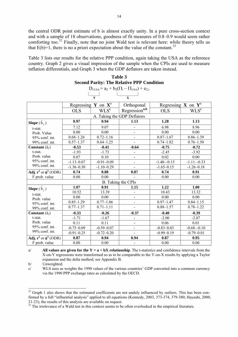
Table 3 lists our results for the relative PPP condition, again taking the USA as the reference country. Graph 2 gives a visual impression of the sample when the CPIs are used to measure inflation differentials, and Graph 3 when the GDP deflators are taken instead.

Table 3 Second Parity: The Relative PPP Condition

Di/USA = a2 + b2(Πi – ΠUSA) + e2,i |_____| |__________| Y X


Orthogonal Regressiona,b OLS WLSc

A. Taking the GDP Deflators 0.97 0.94 1.13 1.28 1.13 7.12 9.07 - 6.98 8.96 0.00 0.00 - 0.00 0.00

0.68–1.26 0.72–1.16 - 0.87–1.67 0.86–1.39

Slope ( ) 2b t-stat. Prob. Value 95% conf. int. 99% conf. int. 0.57–1.37 0.64–1.25 - 0.74–1.82 0.76–1.50

-0.53 -0.41 -0.64 -0.75 -0.72 -1.93 -1.73 - -2.45 -3.92 0.07 0.10 - 0.02 0.00

-1.13–0.07 -0.91–0.09 - -1.40–-0.15 -1.11–-0.33


0.74 0.88 0.87 0.74 0.91 Adj. r2 or φ2 (ODR) F prob. value 0.00 0.00 - 0.00 0.00

B. Taking the CPIs 1.07 0.91 1.15 1.22 1.00

10.52 13.39 - 10.43 13.32 0.00 0.00 - 0.00 0.00

0.85–1.29 0.77–1.06 - 0.97–1.47 0.84–1.15


-0.33 -0.26 -0.37 -0.40 -0.39 -1.71 -1.67 - -2.00 -2.87 0.11 0.11 - 0.06 0.01

-0.75–0.09 -0.59–0.07 - -0.83–0.03 -0.68–-0.10






32 Graph 1 also shows that the estimated coefficients are not unduly influenced by outliers. This has been con-firmed by a full “influential analysis” applied to all equations (Kennedy, 2003, 373-374, 379-380; Hayashi, 2000, 21-23); the results of this analysis are available on request. 33 The irrelevance of a Wald test in this context seems to be often overlooked in the empirical literature.

15

Again, the data do not contradict H0: b=1, the theoretically expected value. The PPP condition in its relative form thus also holds up empirically in the long run, on average and ex post, with a statistically significant intercept in some cases. That the measures of fit (adjusted r2’s for the OLS equations and φ2 for the ODRs) are higher when taking the CPIs is surely due to the di-rect impact of the exchange rate on the CPIs (which includes the prices of imported consumer goods). The GDP deflators are the theoretically more relevant price indices since they are supposed to capture “home-grown” inflation; on the other hand, the CPIs are in general meas-ured more precisely. WLS is more efficient than OLS when estimating PPP, although not for UIP and RIP, which is evident from comparing the respective t-statistics. The estimated con-stants, as noted, are to be discussed in section III.3.

Graph 2: GDP Deflator-Based Purchasing Power Parity

-6

-4

-2

0

2

4

6

-6 -4 -2 2 4 6

GDP DeflatorInflation Differential



Line



Graph 3: CPI-Based Purchasing Power Parity

-6

-4

-2

0

2

4

6

-6 -4 -2 2 4 6




Line

CPI Inflation Differentialvis-à-vis USA, 1976-98

16

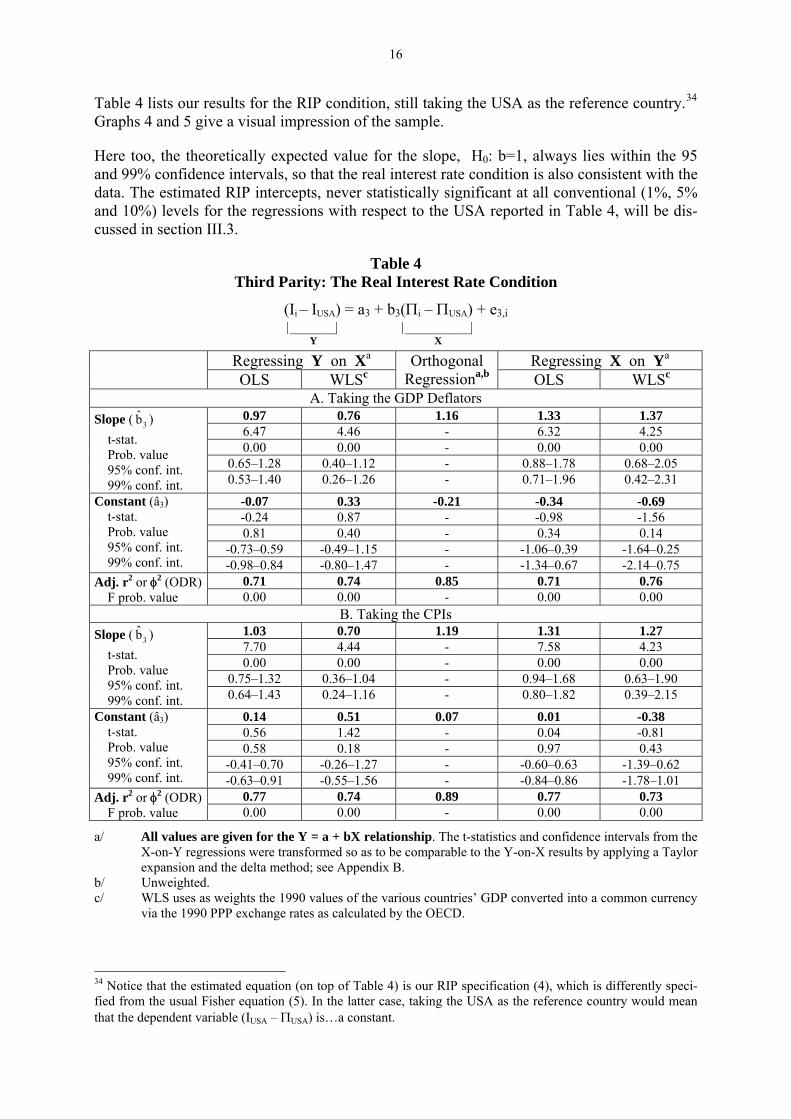
Table 4 lists our results for the RIP condition, still taking the USA as the reference country.34 Graphs 4 and 5 give a visual impression of the sample.

Here too, the theoretically expected value for the slope, H0: b=1, always lies within the 95 and 99% confidence intervals, so that the real interest rate condition is also consistent with the data. The estimated RIP intercepts, never statistically significant at all conventional (1%, 5% and 10%) levels for the regressions with respect to the USA reported in Table 4, will be dis-cussed in section III.3.

Table 4 Third Parity: The Real Interest Rate Condition

(Ii – IUSA) = a3 + b3(Πi – ΠUSA) + e3,i |_______| |__________| Y X


Orthogonal Regressiona,b OLS WLSc

A. Taking the GDP Deflators 0.97 0.76 1.16 1.33 1.37 6.47 4.46 - 6.32 4.25 0.00 0.00 - 0.00 0.00

0.65–1.28 0.40–1.12 - 0.88–1.78 0.68–2.05


-0.07 0.33 -0.21 -0.34 -0.69 -0.24 0.87 - -0.98 -1.56 0.81 0.40 - 0.34 0.14

-0.73–0.59 -0.49–1.15 - -1.06–0.39 -1.64–0.25



B. Taking the CPIs 1.03 0.70 1.19 1.31 1.27 7.70 4.44 - 7.58 4.23 0.00 0.00 - 0.00 0.00

0.75–1.32 0.36–1.04 - 0.94–1.68 0.63–1.90


0.14 0.51 0.07 0.01 -0.38 0.56 1.42 - 0.04 -0.81 0.58 0.18 - 0.97 0.43

-0.41–0.70 -0.26–1.27 - -0.60–0.63 -1.39–0.62






34 Notice that the estimated equation (on top of Table 4) is our RIP specification (4), which is differently speci-fied from the usual Fisher equation (5). In the latter case, taking the USA as the reference country would mean that the dependent variable (IUSA – ΠUSA) is…a constant.

17

Graph 4: GDP Deflator-Based Real Interest Parity

-6

-4

-2

0

2

4

6

-6 -4 -2 2 4 6



GDP DeflatorInflation Differential



Line

Graph 5: CPI-Based Real Interest Parity

-6

-4

-2

0

2

4

6

-6 -4 -2 2 4 6



CPI Inflation Differentialvis-à-vis USA, 1976-98


Line

It was mentioned above that it is not clear from the literature whether real interest rate parity is a separate condition “in its own right”, which should consequently be tested as such. This issue may hinge on which type of agents is doing the arbitrage. For an individual investor residing permanently in a given country, and hence based in that country’s currency, the un-covered nominal interest rate condition is clearly of the essence: she will compare the nominal rate of return on home and foreign assets allowing for the expected path of the nominal ex-change rate; i.e. expected inflation in that investor’s country or abroad will not affect her choice. That may be different for investors who are very mobile internationally and who may therefore be interested in getting the same real returns wherever their investments and they

18

themselves happen to be located at any given time.35 Alternatively, it is conceivable that mul-tinational firms with production facilities and shareholders in many different countries will want to manage their investments, whether financial or material, in such a way that the real rate of return in the different countries is ultimately equalized.36 We shall return to this issue in sections III.3 – III.6.

The triple-parity law therefore says that, except for inter-country financial/institutional and real/structural differentials, the real interest rate should tend to become equalized, on average, in the long run and ex post. This is illustrated in Graph 6.37 It is striking that average real long-term interest rates are very closely bunched around the 4% p.a. value for ten economies out of eighteen, including all the larger ones except Australia and Canada. Country-specific factors seem important for eight countries (shaded area in Graph 6), about which more in the next section where the significance of these deviations will be tested. It is noteworthy that the pattern for nominal interest rates (Graph 7) is quite different from that for real interest rates (Graph 6), and that the former are more widely spread out than the latter.

Graph 6

0

2

4

6

8

10

12

14

A F D I J NZ E S GB

USA

AUSBCDN

CH

DKSF NL N

% p.a. 1976-1998 Average Real Long-Term Interest Rates Using GDP Deflators

Mean = 4.52 S. D. = 1.16

35 On this, see Marston (1997). 36 Obstfeld-Taylor (2000, 1) offer another explanation: “International real interest rate equality would hold in the long run in a world where capital moves freely across borders and technological diffusion tends to drive a con-vergence process for national production possibilities.” 37 Countries are identified by the country tags one sees on automobiles: A = Austria; F = France; D = Germany; I = Italy; J = Japan; NZ = New Zealand; E = Spain; S = Sweden; GB = United Kingdom; USA = United States of America; AUS = Australia; B = Belgium; CDN = Canada; CH = Switzerland; DK = Denmark; SF = Finland; NL = Netherlands; N = Norway.

19

Graph 7

0

2

4

6

8

10

12

14

A

F

D

I

J

NZE

SGB

USA

AUS

BCDN

CH

DK

SF

NL

N

1976-1998 Average Nominal Long-Term Interest Rates % p.a.

Mean = 9.33 S. D. = 2.20

III.3 The Country-Specific Intercepts: Interpretation as Comparative (Dis)Advantages

In this section, we shall look at the statistically significant deviations from the triple-parity law which we observe in the case of some countries – actually, a small number of small coun-tries, as will be seen. In some sense, these cases should therefore be considered as anomalies which do not gainsay the general validity of the triple-parity law. Prior to that, some further considerations on our estimation methods are in order.

So far, the USA has been taken as the reference country, which is an arbitrary although per-haps natural choice. If another country is selected as the reference one, so that all differentials are computed with respect to that other country, it will change the estimated constants, but not the estimated gradients and their associated statistics, which remain exactly the same as in the above tables. In other words, the choice of the reference country makes no difference for the estimated b coefficients, but it does for the constants. Given the way the different variables are defined, all equations are really log-log ones. If the measurement unit of one or several variables is changed in a log-log equation, it will alter the estimated constant only. Thus, changing the reference country is similar to changing the measurement unit.

This issue however calls for some additional explaining. When estimating any one among our equations, a natural impulse would be to take as a sample the various differentials for 17 countries out of a total of 18, i.e. omit the reference country altogether. If this is done, the various b estimates however turn out to be different, depending on which country is taken as the reference one, although the differences are always very small; in particular, the relevant 95% confidence intervals always overlap and all always include the unit value for the esti-mated b’s. In effect, the triple-parity law is therefore not falsified. It is however disturbing from a theoretical standpoint that the – purely “nominal” – choice of the measurement unit should have an effect on the estimated slopes, no matter how small it may be. But if each relevant sample is extended to include the reference country, whose differentials are identi-

20

cally equal to zero, which is what has been done for the estimations in tables 2-4,38 the theo-retically expected result obtains: the estimated slopes and all associated statistics are then ex-actly the same whatever country is selected as the reference one. The best way we can think of to justify this point is by means of an analogy.

Image a pure barter economy. One good is selected as the numéraire, its price being identi-cally equal to one. We then have a vector of real prices for all goods. Now suppose we want to find out whether there is any significant relationship between the price vector and some other vectors measuring, for example and among other relevant factors, the degree of compe-tition in the various goods markets. There would then be no reason to omit the price of the numéraire good: although it is identically equal to unity, it conveys information that should not be arbitrarily thrown away and it should therefore be included in the sample. By analogy, there is no more reason to exclude the reference country from our various samples.39 But to repeat: its inclusion or exclusion has no impact on the general empirical validity of the triple-parity law.

Including the zero differentials for the reference country also has an interesting econometric consequence. Take any equation where the USA is the reference country. Given that both the right-hand side (RHS) and left-hand side (LHS) variables are zero for the USA, the estimated constant must by necessity be equal to the residual for the USA, with the sign reversed.40 The same obtains when each one of the other countries is taken in turn as the reference country. Consequently, the various estimated constants and the various reference-country own residu-als are one and the same thing, and we do not need to show them separately.41 Table 5 lists them for the first equation, i.e. the uncovered nominal interest rate parity condition.

Each estimated constant includes – but is not necessarily equal to – the average country-specific financial/institutional premium. This is so because an estimated constant can be non zero for three non mutually exclusive reasons: (1) E(ei) = some constant ≠ 0: the measurement errors affecting the dependent variable include a systematic bias which will show up in the estimated intercept; (2) even when E(ei)=0, genuinely random shocks will in general not aver-age out to zero in any finite sample; (3) there is a non zero average risk premium differential or financial/institutional disadvantage, in a broad sense, for the country under consideration. Given that our cross-section is made up of trend or mean values for a 23-year period, reason (2) is unlikely to be important. Reason (1) could however be important if the dependent vari-able is affected by measurement errors with a sizable bias. This caveat should be borne in mind when examining the results listed in Table 5 – especially, it would seem, those for the Y-on-X regressions, since appreciation/depreciation rates are likely to be measured with a high degree of precision, but not so our long-term interest rate series, as argued previously.42

38 Also see graphs 1-5. 39 Since our equations are really log-log ones, a zero differential is similar to the unit price for the numéraire good in our analogy: the anti-log of zero is one. 40 Given yi = â1 + x1b i + ê1,i, yi = xi = 0 means â1 = – ê1,i. 41 Take any one of our cross-section equations: although the estimated constant and the reference-country own residual are one and the same thing in that given equation, this leaves the residuals for the other countries. Ide-ally, all these cross-section residuals should be checked as to their randomness, but – to our knowledge – no such explicit tests are available in a pure cross-section context, and only “eyeballing” can be resorted to. We have closely scrutinized the residuals for all equations and have found no indication of non randomness. E.g. it is never the case that large countries tend to have small residuals, and small countries large residuals, etc. The vari-ous residual series and the corresponding graphs are available on request. 42 On the other hand, the reverse X-on-Y regressions would then suffer from a serious error-in-data problem, meaning that the slope estimates might be biased – and hence also the estimated constants. Consider a two-

21

Table 5 Nominal UIP: The “F”-Differentials or Financial/Institutional Disadvantages

Estimated Constants or Own-Country Residuals, in Percentage Pointsb

Y-on-X Regressionc X-on-Y Regressionc

OLS WLS OLS WLS

Reference Countrya

â1 p-value â1 p-value â1 p-value â1 p-value

Switzerland -1.60 0.01 -1.02 0.28 -2.44 0.00 -3.55 0.00 Sweden -1.09 0.00 -0.98 0.00 -0.89 0.04 -0.90 0.05 Australia -0.95 0.00 -0.88 0.00 -0.66 0.12 -0.59 0.21 New Zealand -0.72 0.02 -0.66 0.02 -0.39 0.31 -0.28 0.50 Canada -0.40 0.08 -0.24 0.33 -0.31 0.25 -0.45 0.15 USA -0.39 0.09 -0.14 0.68 -0.50 0.05 -0.84 0.01 Norway -0.37 0.11 -0.23 0.35 -0.25 0.36 -0.35 0.25 UK -0.19 0.40 -0.03 0.91 -0.10 0.69 -0.23 0.45 France -0.01 0.98 0.18 0.50 0.04 0.87 -0.14 0.66 Spain 0.01 0.97 -0.01 0.98 0.50 0.13 0.79 0.00 Germany 0.07 0.83 0.46 0.42 -0.35 0.27 -1.01 0.07 Italy 0.09 0.81 0.05 0.90 0.62 0.07 0.95 0.00 Netherlands 0.40 0.16 0.74 0.13 0.09 0.78 -0.46 0.43 Belgium 0.50 0.03 0.73 0.03 0.44 0.12 0.15 0.73 Austria 0.62 0.04 0.97 0.06 0.30 0.43 -0.27 0.68 Finland 0.63 0.02 0.72 0.01 0.87 0.00 0.91 0.00 Japan 1.47 0.00 1.97 0.02 0.80 0.24 -0.12 0.92 Denmark 1.93 0.00 2.00 0.00 2.23 0.00 2.32 0.00

a/ In ascending order for the OLS direct regression. b/ Shaded values are significant at the 5% level. c/ All values are given for the Y = a + bX relationship.

Perhaps the most striking thing about the results in Table 5 is that they are quite sensitive to the direction of regression and to the estimation method (OLS vs WLS), as the correlation (ρ) matrix in Table 6 confirms.

Table 6 Correlation Matrix for the Alternative UIP “F”-Differential Estimates (in Table 5)

ρ Y on X OLS Y on X WLS X on Y OLS X on Y WLS Y on X OLS 1.00 Y on X WLS 0.98 1.00 X on Y OLS 0.91 0.82 1.00 X on Y WLS 0.74 0.60 0.95 1.00

This sensitivity to the direction of regression and the estimation method is even more notice-able when considering the statistical significance of the estimated constants: had we limited ourselves to the direct OLS regressions, i.e. the first â1 vector in Table 5, we would have con-cluded that the intercept is significant (at the 5% level) for 9 countries out of 18: Switzerland,

variable, linear and upward-sloping equation: if the estimated slope is biased, say, upwards, the estimated con-stant will necessarily be biased downwards.

22

Sweden, Australia, New Zealand, Belgium, Austria, Finland, Japan and Denmark – all of them small economies, except Australia and Japan.

However, looking across the various â1’s for each country, and admitting as a rule of thumb that there are “strong indications” of an overall significant intercept when the â1’s are signifi-cant in at least three cases out of our four estimates, we find relevant results for four small countries only: Switzerland, Sweden, Finland and Denmark – the latter two being the only ones for which the constants are in all cases significantly different from zero. Moreover, the four point estimates are closely bunched for Sweden, Finland and Denmark, but not for Swit-zerland. This illustrates the importance of the regression direction and estimation method is-sues when using single-equation techniques.

Bearing in mind the preceding caveats about possible error-in-data problems, a negative inter-cept is indicative of a risk premium differential for the country under consideration or, more generally, of a financial/institutional comparative advantage, as argued previously. This is best seen when considering the reverse relationship: a negative constant means that, for a given rate of depreciation/appreciation, and for a given level of foreign nominal interest rates, said country enjoys domestic interest rates that are lower than would be expected normally.43 Seen in this light, the results in Table 5 suggest that Switzerland and Sweden have likely benefited from an important international comparative advantage whereas Finland and Den-mark appear to have been at a sizable disadvantage.

Why this should be so for these four countries will be discussed further on when examining the constants in the real interest rate parity equations. A proviso should however be stated right away: if the risk premium – or financial/institutional disadvantage – for a given country has remained constant over the sample period, the interpretation (e.g. in terms of structural factors, policies, etc.) is likely to be more straightforward than if it has been changing. Neither will there be a specific econometric problem on this account. If the risk premium – or finan-cial/institutional disadvantage – has changed over time, but without being correlated with the independent variable, no specific econometric problem arises either; yet the estimated con-stant is then a measure of the average risk premium over the sample period and it says noth-ing about what it might be today or in recent years. In the case of the direct regressions, the national interest rates are widely fluctuating but (theoretically) likely to be stationary series whereas the risk premium is likely to change – if it changes at all – slowly and smoothly over time, and the two are therefore unlikely to be significantly correlated. We have a problem if (a) the changing risk premium and the interest rate differentials nevertheless happen to be corre-lated;44 and/or (b) if, as stated above, E(ei) = some (sizable) constant ≠ 0 (i.e. measurement error with bias).

We now turn to the estimated constants in the PPP equations, reported in Table 7.

43 Taking the direct relationship, a small constant means that the country benefits from a stronger (i.e., more rapidly appreciating) currency than would be expected given its interest rate level relative to foreign interest rates. Bear in mind that we are considering a long-term equilibrium situation, so that no competitiveness prob-lems arise due to a currency which appreciates more rapidly than one would normally expect. This means that, for a given volume of exports, the country can import more cheaply from abroad without running into balance-of-payments problems. 44 For the reverse regressions: if the changing risk premium is correlated with the depreciation rate.

23

Table 7 Relative PPP: The “R”-Differentials or Real/Structural Advantages



OLS WLS OLS WLS

Reference Countrya


Australia -2.55 0.00 -2.45 0.00 -2.58 0.00 -2.64 0.00 Canada -1.51 0.00 -1.39 0.00 -1.71 0.00 -1.69 0.00 Norway -1.08 0.00 -0.98 0.00 -1.11 0.02 -1.17 0.00 Sweden -0.75 0.03 -0.69 0.00 -0.31 0.51 -0.60 0.03 USA -0.53 0.07 -0.41 0.10 0.75 0.02 -0.72 0.00 Netherlands -0.42 0.34 -0.25 0.53 -1.18 0.00 -0.88 0.01 Belgium -0.24 0.42 -0.12 0.67 -0.57 0.07 -0.49 0.05 Finland -0.11 0.68 -0.03 0.87 0.05 0.88 -0.11 0.56 France 0.02 0.93 0.12 0.51 0.10 0.73 -0.01 0.95 New Zealand 0.12 0.79 0.15 0.53 0.91 0.02 0.44 0.02 Denmark 0.39 0.15 0.49 0.02 0.40 0.22 0.32 0.20 Germany 0.44 0.23 0.59 0.09 -0.12 0.78 0.08 0.84 UK 0.46 0.14 0.53 0.00 0.82 0.01 0.57 0.00 Spain 0.75 0.18 0.75 0.02 1.78 0.00 1.20 0.00 Austria 0.90 0.01 1.04 0.00 0.45 0.36 0.60 0.19 Switzerland 1.09 0.01 1.14 0.00 0.56 0.32 0.74 0.15 Italy 1.15 0.07 1.23 0.00 2.35 0.00 1.69 0.00 Japan 1.86 0.00 2.04 0.00 0.90 0.31 1.29 0.11


The previous caveats about the three possible reasons for non zero intercepts should be kept in mind so that not too much should be read into our results. With that proviso, a significant negative constant for a given country in Table 7 is indicative of unfavorable real/structural disadvantage (in a comparative perspective), and vice-versa – be it a constant factor or an average over the sample period. Applying the same rule of thumb as previously, four coun-tries appear to exhibit real/structural disadvantage: Australia, Canada, Norway and Sweden, all of them important producers and exporters of primary commodities and raw materials. The estimated intercept is significant in all four cases and the point estimates lie close to one an-other. At the other end, real/structural advantages have been enjoyed in the UK, Spain and Italy. The point estimates are closely bunched for the UK, but are small. They are larger for Spain and Italy, but also rather spread out. The explanation may be that these three countries have undergone especially rapid modernization in the sample period (the UK under and after Mrs. Thatcher).

Similar general comments apply to our results in Table 8, i.e. the constants in the equations for the real interest rate parity conditions.45 Using the same rule of thumb as above, we now find that six countries appear to be at a statistically significant overall comparative advantage 45 In Table 8, the sign of the estimated intercepts has been reversed (for the equations used, see top of Table 4) so as to make a small (i.e., negative) value correspond to a comparative advantage, as was the case for the nominal interest rate equations. This is not done in Table 9, hence RIP premia vs RIR discounts in the titles of these ta-bles.

24

(Switzerland, the UK) or disadvantage (Belgium, Finland, Denmark and Australia). The point estimates are however closely bunched only in the case of Finland, Denmark and Australia.

Table 8 RIP: The Combined “F” and “R” Differentials, Overall Disadvantages or RIR Premia



OLS WLS OLS WLS

Reference Countrya


Switzerland -3.19 0.00 -3.80 0.00 -2.56 0.05 -2.17 0.18 Japan -0.80 0.16 -1.70 0.04 0.36 0.58 0.79 0.45 Italy -0.73 0.28 -0.17 0.77 -2.18 0.00 -1.97 0.00 Germany -0.63 0.13 -1.27 0.03 0.05 0.93 0.44 0.58 New Zealand -0.63 0.20 -0.35 0.36 -1.58 0.00 -1.33 0.00 UK -0.59 0.10 -0.61 0.03 -1.02 0.01 -0.72 0.04 Austria -0.48 0.20 -1.03 0.05 0.06 0.88 0.44 0.52 Spain -0.43 0.47 0.02 0.97 -1.67 0.00 -1.45 0.02 Sweden -0.22 0.54 -0.18 0.52 -0.75 0.04 0.46 0.19 France 0.00 0.99 -0.20 0.48 -0.10 0.77 0.23 0.56 USA 0.07 0.81 -0.33 0.40 0.34 0.33 0.69 0.14 Netherlands 0.62 0.20 -0.15 0.82 1.54 0.00 1.95 0.00 Belgium 0.70 0.04 0.23 0.61 1.10 0.01 1.46 0.00 Norway 0.78 0.01 0.51 0.13 0.81 0.06 1.15 0.01 Finland 0.89 0.01 0.75 0.01 0.69 0.15 1.01 0.03 Canada 1.15 0.00 0.76 0.06 1.40 0.01 1.75 0.00 Denmark 1.72 0.00 1.47 0.00 1.72 0.01 2.05 0.00 Australia 1.77 0.00 1.49 0.00 1.81 0.01 2.15 0.00


Looking back at equation (4)-(5), it is seen that the constant in the RIP equation is equal to the real/structural differential in the PPP equation minus the financial/institutional differential in the nominal UIP equation: a country will enjoy a comparative real interest rate advantage (or discount) if its real/structural advantage (traditionally interpreted as productivity growth dif-ferential) is larger than its financial/institutional disadvantage (traditionally interpreted as nominal interest rate risk premium) – an interesting proposition in itself. This also affords us a way to check whether the estimated country-specific constants in the real interest parity equa-tions (Table 8), which we shall call the direct estimates of the “real interest rate (RIR) dis-counts”, are consistent with the differences between the estimated real/structural advantages (Table 7) and the estimated financial/institutional disadvantages (Table 5), these differences to be dubbed here the indirect estimates of the RIR discounts – see Table 9.

25

Table 9 RIR Discounts: Comparing Indirect (UIP + PPP Implied) and Direct (RIP) Estimates

OLS Estimates: Y on X OLS Estimates: X on Y Indirect Direct Differencea Indirect Direct Differencea

Australia -1.60 -1.77 -0.17 Australia -1.92 -1.81 0.11 Austria 0.28 0.48 0.20 Austria 0.15 -0.06 -0.21 Belgium -0.74 -0.70 0.04 Belgium -1.01 -1.10 -0.09 Canada -1.11 -1.15 -0.04 Canada -1.40 -1.40 0.00 Denmark -1.54 -1.72 -0.18 Denmark -1.83 -1.72 0.11 Finland -0.74 -0.89 -0.15 Finland -0.82 -0.69 0.13 France 0.03 0.00 -0.03 France 0.06 0.10 0.04 Germany 0.37 0.63 0.26 Germany 0.23 -0.05 -0.28 Italy 1.06 0.73 -0.33 Italy 1.73 2.18 0.45 Japan 0.39 0.80 0.41 Japan 0.10 -0.36 -0.46 Netherlands -0.82 -0.62 0.20 Netherlands -1.27 -1.54 -0.27 New Zealand 0.84 0.63 -0.21 New Zealand 1.30 1.58 0.28 Norway -0.71 -0.78 -0.07 Norway -0.86 -0.81 0.05 Spain 0.74 0.43 -0.31 Spain 1.28 1.67 0.39 Sweden 0.34 0.22 -0.12 Sweden 0.58 0.75 0.17 Switzerland 2.69 3.19 0.50 Switzerland 3.00 2.56 -0.44 UK 0.65 0.59 -0.06 UK 0.92 1.02 0.10 USA -0.14 -0.07 0.07 USA -0.25 -0.34 -0.09 Mean 0.00 0.00 0.00 Mean 0.00 0.00 0.00 S. D. 1.06 1.15 0.23 S. D. 1.32 1.36 0.26 Correlation coefficient: 0.98 Correlation coefficient: 0.98

a/ Direct minus indirect estimates.

It is evident that the direct and indirect estimates are actually quite close, being highly corre-lated. It is also worth noting that none of the differences between them is larger than half a percentage point.

It might be tempting to argue that if real interest rate equalization is due to a “special” class of arbitraging agents, be they investors or firms (as discussed above), we should rather expect the direct estimates to be different from the indirect ones because these agents’ perceived RIR discounts/premia – i.e. financial/institutional and real/structural (dis)advantages – may be different from that of the other (“non special”) investors or firms. But this ignores that all agents operate on the same (global) financial and goods markets where their interactions re-sult in average market-wide discounts/premia. No matter how we look at it, the deterministic parts of equations (1) and (2) necessarily imply the deterministic part of equation (3)-(4)-(5): if the UIP and PPP equilibrium conditions hold, the RIP condition must hold too. It follows that, seen in this light, the real interest parity condition cannot possibly be a separate condition “in its own right”. However, the issue takes on another meaning if we allow for the possibility that the arbitrage activities of these “special” agents may result in separate shocks, eRIP, so that equation (3) should be rewritten as:

(FA – FB) + (IB A – IBB) = (RB – RA) + (ΠA – ΠB) + (eB 2 – e1) + eRIP. (10) ⏐_____________⏐ = e3

Under these conditions, it is econometrically justified to test the RIP relationship as a separate condition, as we – and others – have done. Furthermore, it is also possible that the existence

26

of this special class of arbitrageurs, supposing it really exists, will reinforce and speed up the realization of the UIP and PPP conditions.

Finally, summing up our results for both the nominal and the real interest rate parity condi-tions, we can conclude that only Denmark, Finland and Switzerland46 appear to constitute significant anomalies on both counts.47 Why should that be so? E.g. why should Finland and Denmark appear to be at a significant disadvantage on both the nominal and the real interest rate count whereas Switzerland would seem to enjoy a significant comparative advantage? In the case of Switzerland, the explanation is most likely to be found in that country’s reputation for political, economic and financial stability, its efficient financial sector – as well as, per-haps, its banking secrecy law and its status as an international tax heaven, although this inter-pretation has been rejected in at least one study.48 As to Finland and Denmark, the reasons may be of different, rather structural nature, as suggested in the next paragraph.

For all three countries, an important issue is whether or not their relative RIR dis-counts/premia have been more or less stationary over the sample period. Graph 8 sheds some light on this issue, focusing on the annual evolution of ex post real long-term interest rates (notice the different scales). The graph suggests that Switzerland’s low RIR premium is a permanent factor whose expected value may have been approximately constant over the sam-ple period. In the case of Denmark, its high average RIR premium appears to be linked with high real interest rates in the 1980s and in the first half of the 1990s: the Danish economy was then very inflationary and the crown under constant attack; but the problem seems to have been solved in more recent years. As to Finland, its high average RIR premium may be due mostly to disruptions in the late 1980s and early 1990s following the collapse of the Soviet Union, which used to absorb a fair share of Finish exports; but there too the problem seems to be on the mend.

Graph 8: Long-Term Real Interest Rates in Switzerland vs Denmark and Finland

-2

-1

0

1

2

3

4

5

76 78 80 82 84 86 88 90 92 94 96 98

% p

.a.

Switzerland: CPI-Defined Real Interest Rate

-2

-1

0

1

2

3

4

76 78 80 82 84 86 88 90 92 94 96 98

% p

.a.

Switzerland: GDP Deflator-Defined Real Interest Rate

46 Switzerland being so special appears not strange at all: Koedijk-Tims-Van Dijk (2004), for instance, have recently found similar conclusions in their PPP tests for the Euro area, where the only exception has been the Swiss franc. 47 To be more precise: there is significant econometric evidence that these three countries constitute anomalies. Other countries may be anomalous too, but our data may not enable us to identify them. 48 See Commission pour les questions conjoncturelles (2003). Here is not the place to go into the pros and cons of the latter two institutional factors, except maybe to point out that if there are cons (e.g. both institutional fac-tors may be abused by non Swiss tax evaders), there are also pros (e.g. protection of the private sphere and safe-guard against extortionate national tax laws).

27

0

2

4

6

8

10

76 78 80 82 84 86 88 90 92 94 96 98

% p

.a.

Finland: CPI-Defined Real Interest Rate

0

2

4

6

8

10

12

76 78 80 82 84 86 88 90 92 94 96 98

% p

.a.

Finland: GDP Deflator-Defined Real Interest Rate

2

4

6

8

10

76 78 80 82 84 86 88 90 92 94 96 98

% p

.a.

Denmark: GDP Deflator-Defined Real Interest Rate

2

4

6

8

10

12

76 78 80 82 84 86 88 90 92 94 96 98

% p

.a.

Denmark: CPI-Defined Real Interest Rate

III.4 System Estimation Methods: SUR and FIML Results

Besides the single-equation methods reported thus far, OLS, WLS and ODR, the triple-parity law has also been estimated as a system. To do so, we applied two alternative and comple-mentary techniques, namely Zellner’s (1962) seemingly unrelated regressions (SUR) estima-tor and full information maximum likelihood (FIML), with Marquardt’s algorithm. For rea-sons that will be seen presently, the SUR and FIML methods must be discussed together.

To justify our use of the mentioned econometric techniques, we would first of all recall that system estimation seems more relevant in our context where we regard the triple parity as a joint law. System methods would utilize more information, namely across equations, in esti-mating the coefficients of interest and are thus likely to be better in terms of efficiency. In particular, SUR is relevant under the assumption that the error terms in the UIP, PPP and RIP equations are contemporaneously correlated, a hypothesis that appears realistic. Moreover, the SUR estimator is known to be more efficient than equation-by-equation OLS when the vari-ance-covariance matrix of the system is not diagonal, which is very likely too (or when the explanatory variables are not the same, which is the case in our system estimation by pairs of parities as reported below). If, on the contrary, the errors in the three equations are not corre-lated but are independent, we can replace – or rather complement – our SUR estimates with

28

simultaneous equations models (SEM). Assuming – and also checking49 – that these distur-bances are normally distributed, a particular version of SEM that is commonly applied is FIML. Complementing SUR by FIML estimates thus ensures robustness for our results under alternative underlying assumptions as to the shocks to UIP, PPP and RIP.

SUR can, however, perform poorly when the error contemporaneous variance-covariance matrix is not precisely estimated (via the OLS residuals by equation), as noted by Kennedy (2003, 199) among others. Following this caveat and the usual recommendation on how to proceed, we also re-estimated our OLS regressions with White’s heteroskedasticity-consistent correction, since when the USA-based equations were checked for heteroskedasticity, a few tested positive.50 The re-estimated b coefficients were not changed hereby, of course, but their standard errors were: the latter turn out to be somewhat larger in some cases and somewhat smaller in others, but all the confidence intervals continue to support the basic E(b)=1 hy-pothesis – and hence the triple-parity law.

FIML has the nice property of invariance (see, for instance, Hayashi 2000, 534). I.e. the ques-tion does not arise as to how the equations are to be normalized, and hence neither does the direction-of-causality issue. In the present case, this method however raises a number of in-triguing questions. To discuss them, let us simplify our notation and rewrite our three basic relationships as a system of equations:

DUSAi = c(1) + c(2)*IUSAi + e1,i, (11)

i.e. the uncovered nominal interest rate parity condition (the UIP equation), with DUSAi = average depreciation rate of country i’s currency with respect to the dollar, and IUSAi = i’s average nominal interest differential vis-à-vis the USA,

DUSAi = c(3) + c(4)*ΠUSAi + e2,i, (12)

i.e. the relative PPP condition (the PPP equation), with ΠUSAi = country’s i’s average infla-tion rate differential with respect to the USA,

IUSAi = c(5) + c(6)*ΠUSAi + (e1,i – e2,i) + eRIP,i, (13)

i.e. the real interest rate parity condition (the RIP equation).

Obviously, c(1), c(3), (c5) correspond, respectively, to the slopes a1, a2, a3, and c(2), c(4), c(6) to b1, b2, b3. Assuming that these three equations represent three independent arbitrage mechanisms, and in particular that the third one is not simply the result of combining the first two (it includes e3,i as per the preceding discussion), they make up a closed system: all vari-ables (= differentials) are endogenous, there are no exogenous variables which could be used as instruments, and hence no reduced form. Consequently, the FIML method cannot be ap-plied to our full system of three equations. If we want to use FIML, we must instead take them two by two, for a total of three combinations.

49 The null of normality of the residuals from the direct and reverse UIP, PPP and RIP OLS regressions could not be rejected by the Jarque-Bera tests we performed at the 10% significance level for none of the total of 10 speci-fications (including PPP and RIP being alternatively estimated from CPIs or GDP deflators) and for 8 of the tests at the 20% level. Results are available on request. 50 Given that the general triple-parity law has to do with the b coefficients, and that these do not change when the reference country is changed, only the USA-based OLS equations were tested.

29

Doing this however reintroduces the question of normalization, and hence that of the direction of causality. If, for example, we try to apply FIML to (11) and (12) as normalized above, i.e. with the same dependent variable, the algorithm breaks down. It is easy to see why: both equations have only one exogenous variable on their RHS, so trying to estimate them by FIML is pointless.

The system (11)-(12) must therefore be renormalized, which can be done in two ways:

DUSAi = c(1) + c(2)*IUSAi + e1,i, (14)

ΠUSAi = – [c(3)/c(4)] + [1/c(4)]*DUSAi – [1/c(4)]*e2,i, (15)

or

IUSAi = – [c(1)/c(2)] + [1/c(2)]*DUSAi – [1/c(2)]*e1,i, (16)

DUSAi = c(3) + c(4)* ΠUSAi + e2,i. (17)

Both systems are recursive; or they are only triangular if the two e’s are not independent,51 as might well be the case. Let us consider the two systems’ deterministic parts. In the first one, for example, IUSAi is exogenous and determines DUSAi via (14), and then ΠUSAi is deter-mined by DUSAi via (15).52 Since (14) comprises no endogenous variable on its RHS, the FIML point estimates of c(1) and c(2) will be exactly the same as those given by OLS (al-though the standard errors will be different). The FIML point estimates of c(3) and c(4) in (15) will however be different from the OLS ones. Given that the deterministic parts of (14)-(15) make up a triangular system, these FIML-estimated coefficients will also be identical to the SUR estimates (although the standard errors will again be different).

The situation is reversed for the system (16)-(17). The FIML point estimates of c(3) and c(4) will now be identical to the OLS ones, while those for c(1) and c(2) will be SUR/FIML point estimates different from the OLS ones.

Consequently, our SUR/FIML point estimates will be those

• given by (16)-(17) for c(1) and c(2), and those • given by (14)-(15) for c(3) and c(4),

and we need not reproduce the OLS point estimates again.

The same reasoning holds for the other two combinations of equations (11)-(13) taken two by two.53 Table 10 gives the results for all three combinations.

51 And so is the system (11)-(13) if (11) is renormalized so as to determine CPUSAi – see below. 52 Notice that, by the order condition, both equations are exactly identified. 53 Combination (11) and (13) can be estimated as it is because the system is triangular. For the reasons indicated in the text, the estimated coefficients (but not the standard errors) for (13) will be the same as the OLS direct-regression ones in Table 4.

30

Table 10 Triple Parity: SUR/FIML Pairwise Resultsa

Estimated equations taken two by twob

Slope ( ) b

Constant (â)

Adj. r2

(11) UIP (12) PPP

1.00 (10.3; 3.0)

(0.098; 0.332) 1.20

(8.0; 4.6) (0.149; 0.261)

–0.46 (–2.1; –1.1) (0.21; 0.43)

–0.69 (–2.4; –1.4)

(0.282; 0.490)

0.82

0.74

(11) UIP (13) RIP

1.00 (10.9; 3.0)

(0.092; 0.332) 1.19

(7.7; 3.6) (0.155;0.331)

–0.46 (–2.1; –1.1)

(0.213; 0.434) –0.23

(–0.8; –0.5) (0.304; 0.445

0.82

0.70

(12) PPP (13) RIP

1.20 (9.9; 4.6)

(0.121; 0.261) 1.19

(8.9; 3.6) (0.134; 0.331)

–0.69 (–2.5; –1.4)

(0.276; 0.490) –0.23

(–0.8; –0.5) (0.299; 0.445)

0.70

0.66

a/ t-statistics (second line) and standard errors (third line) in parentheses below coefficients; first figure: SUR; second: FIML.

b/ All results are given for the Y-on-X specification. Inflation differentials from GDP deflators. Country of reference: USA. SUR: simultaneous weighting matrix and coefficient iteration.

Comparing these results for any given relationship (say, UIP), it is seen that the SUR/FIML estimated coefficients are not affected by whichever combination is selected, but their stan-dard errors are. The normalization or direction-of-causality issue is therefore irrelevant on the first count, but not on the second one. Furthermore, it is seen that the SUR method leads to t-statistics that are noticeably higher than those from FIML, which is as expected. It is true that the RHS variables in our SUR system are not strictly exogenous but rather predetermined endogenous, so that their use as regressors may lead to some bias in the reduced-form esti-mates. Yet Kennedy (2003, 192) notes that these estimates should nevertheless be asymptoti-cally unbiased, assuming the errors are not autocorrelated, and that all estimators in a struc-tural SEM context are anyway biased so that the choice among them is based on their asymp-totic properties. Comparing the results in Table 10 with the OLS ones in tables 2, 3 and 4 also shows that using system estimation methods leads to a significant improvement: 54 the SUR/FIML point estimates lie between the bounds defined by the direct and reverse OLS regressions and they are actually close to the “central” ODR point estimates; on top of that, standard errors and t-statistics are now available, which was not the case for the ODR results. To sum it up: the SUR/FIML methods afford even stronger evidence in favor of the triple-parity law.

As stated above, the three-equation system (11)-(13) cannot be estimated as such by FIML, because it is a closed one, but it can be estimated by SUR if (12) is renormalized so as to de-

54 There is however a (small) price to be paid: the adjusted r2’s are lower with SUR/FIML than with OLS; but they are only slightly lower and remain comfortingly high in a cross-section context.

31

termine ΠUSAi, thus making the deterministic parts of (11)-(13) a fully triangular system – see Table 11, which also gives the OLS results for comparison purposes.

Table 11 Triple Parity: Full System SUR vs OLS Resultsa

SUR Results OLS Resultsb

Equation Slope ( ) b Constant (â) Adj. r2 Slope ( ) b Constant (â) Adj. r2

(11) UIP

0.97 (11.2) (0.086)

–0.43 (–2.1)

(0.206)

0.82 0.90 (9.1)

(0.099)

–0.39 (–1.8)

(0.219)

0.83

(12) PPPP

c

1.14 (9.5)

(0.121)

–0.65 (–2.5)

(0.263)

0.73 1.28 (7.1)

(0.180)

–0.75 (–2.3)

(0.321)

0.75

(13) RIP

1.13 (9.4)

(0.119)

–0.19 (–0.7)

(0.278)

0.69 0.97 (6.5)

(0.149)

–0.07 (–0.2)

(0.300)

0.71

a/ t-statistics (second line) and standard errors (third line) in parentheses below coefficients. Inflation dif-ferentials from GDP deflators. Country of reference: USA. SUR: one-step weighting matrix and coeffi-cient iteration.

b/ See tables 2 and 4 (direct OLS regressions for UIP and RIP) and Table 3 (reverse OLS regression for PPP).

c/ Renormalized – see text. Equation estimated as: ΠUSA = – (c(3)/c(4)) + (1/c(4))*DUSA.

It is seen that for the UIP and PPP equations, but not for the RIP one, the SUR point estimates of the slopes are closer to the theoretically expected values than the OLS point estimates. The SUR-produced t-statistics are also noticeably larger in absolute value than the OLS ones, i.e. the SUR point estimates are better assured, while the adjusted r2’s are only slightly smaller. As the standard errors show, the basic E(b)=1 hypotheses stand up under SUR too. Finally, the SUR full-system results in Table 11 are also distinctly better than the SUR/FIML two-equations-at-a-time results in Table 10, in the sense that the standard errors for the slope coef-ficients are smaller.

III.5 Is RIP Independent of UIP and PPP in the “Long Run”? Econometric Tests

We now return to the question whether RIP is a condition in itself, separate and independent of the arbitrage forces acting jointly through UIP and PPP. One way to answer this question, still unsettled in the literature, is to examine our cross-section regression residuals. To that end, we compute the indirect estimates of the residuals for the RIP equation, i.e. those implied jointly by the residuals of the UIP and PPP equations, and then compare them with the direct ones, as shown in the Table 12.

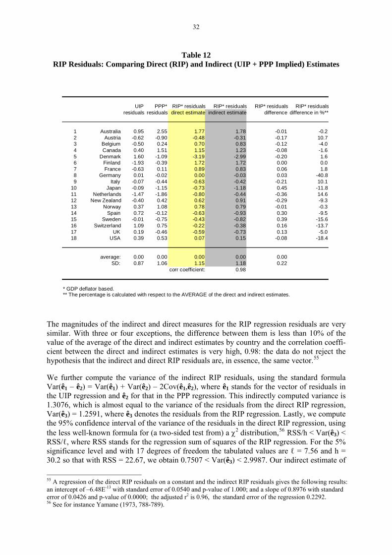
32

Table 12 RIP Residuals: Comparing Direct (RIP) and Indirect (UIP + PPP Implied) Estimates

UIP PPP* RIP* residuals RIP* residuals RIP* residuals RIP* residuals

residuals residuals direct estimate indirect estimate difference difference in %**

1 Australia 0.95 2.55 1.77 1.78 -0.01 -0.22 Austria -0.62 -0.90 -0.48 -0.31 -0.17 10.73 Belgium -0.50 0.24 0.70 0.83 -0.12 -4.04 Canada 0.40 1.51 1.15 1.23 -0.08 -1.65 Denmark 1.60 -1.09 -3.19 -2.99 -0.20 1.66 Finland -1.93 -0.39 1.72 1.72 0.00 0.07 France -0.63 0.11 0.89 0.83 0.06 1.88 Germany 0.01 -0.02 0.00 -0.03 0.03 -40.89 Italy -0.07 -0.44 -0.63 -0.42 -0.21 10.1

10 Japan -0.09 -1.15 -0.73 -1.18 0.45 -11.811 Netherlands -1.47 -1.86 -0.80 -0.44 -0.36 14.612 New Zealand -0.40 0.42 0.62 0.91 -0.29 -9.313 Norway 0.37 1.08 0.78 0.79 -0.01 -0.314 Spain 0.72 -0.12 -0.63 -0.93 0.30 -9.515 Sweden -0.01 -0.75 -0.43 -0.82 0.39 -15.616 Switzerland 1.09 0.75 -0.22 -0.38 0.16 -13.717 UK 0.19 -0.46 -0.59 -0.73 0.13 -5.018 USA 0.39 0.53 0.07 0.15 -0.08 -18.4

average: 0.00 0.00 0.00 0.00 0.00 SD: 0.87 1.06 1.15 1.18 0.22

corr coefficient: 0.98

* GDP deflator based. ** The percentage is calculated with respect to the AVERAGE of the direct and indirect estimates.

The magnitudes of the indirect and direct measures for the RIP regression residuals are very similar. With three or four exceptions, the difference between them is less than 10% of the value of the average of the direct and indirect estimates by country and the correlation coeffi-cient between the direct and indirect estimates is very high, 0.98: the data do not reject the hypothesis that the indirect and direct RIP residuals are, in essence, the same vector.55

We further compute the variance of the indirect RIP residuals, using the standard formula Var(ê1 – ê2) = Var(ê1) + Var(ê2) – 2Cov(ê1,ê2), where ê1 stands for the vector of residuals in the UIP regression and ê2 for that in the PPP regression. This indirectly computed variance is 1.3076, which is almost equal to the variance of the residuals from the direct RIP regression, Var(ê3) = 1.2591, where ê3 denotes the residuals from the RIP regression. Lastly, we compute the 95% confidence interval of the variance of the residuals in the direct RIP regression, using the less well-known formula for (a two-sided test from) a χ2 distribution,56 RSS/h < Var(ê3) < RSS/ℓ, where RSS stands for the regression sum of squares of the RIP regression. For the 5% significance level and with 17 degrees of freedom the tabulated values are ℓ = 7.56 and h = 30.2 so that with RSS = 22.67, we obtain 0.7507 < Var(ê3) < 2.9987. Our indirect estimate of

55 A regression of the direct RIP residuals on a constant and the indirect RIP residuals gives the following results: an intercept of –6.48E-13 with standard error of 0.0540 and p-value of 1.000; and a slope of 0.8976 with standard error of 0.0426 and p-value of 0.0000; the adjusted r2 is 0.96, the standard error of the regression 0.2292. 56 See for instance Yamane (1973, 788-789).

33

the variance of the RIP residuals, Var(ê1 – ê2) = 1.3076, is thus not only very close to the di-rect estimate, Var(ê3) = 1.2591, but it is also well inside the computed 95% confidence inter-val. Such econometric evidence implies that the source of independent shocks in the RIP equation (10), eRIP, is not important. Consequently, we conclude that our data do not reject the hypothesis that RIP results from the joint operation of UIP and PPP not just in a deterministic sense, but also in a statistical one, namely that e3 ≈ e1 – e2.

However, analysis concerns the very “long run” period of 23 years, 1976-1998. Can we say the same for shorter “long run” periods? Put otherwise, how fast is the speed of convergence, through the forces of arbitrage in asset and goods markets, for the three mutually dependent parity conditions bundled up here in the triple-parity law?

III.6 How Long is the “Long Run”? Speed of Convergence for the Triple-Parity Law

To address this question we compute the slope estimates and their 95% confidence interval in the same way as above, but now at successive cumulative sample horizons, starting with a short “long run” (or “medium term”) of 5 years (1976-1980) and then iteratively moving on to progressively longer “long runs” until we reach the end of the sample (1976-1998). The re-sults of these computations are presented in Graph 9.

It is thus confirmed that in the very “long run” of 23 years (1976-1998) all three conditions – UIP, PPP and RIP – hold convincingly: all three regressions result in slope estimates practi-cally equal to 1 at the end of the sample horizon (see the LHS column of diagrams in Graph 9). The 95% confidence interval widths at the same point in time are of the order of 0.4-0.6 (see the RHS column of diagrams in Graph 9).

This is however not the case, especially for the RIP equation, over all or most of the shorter cumulative horizons. Comparing the speed of convergence to the ultimate equilibrium points to some differences and, in particular, casts doubt on the (complete) dependence of the RIP on the joint action of UIP and PPP in shorter “long run” periods. More precisely, taking the 95% confidence band as indicative and looking at the three LHS diagrams, one can see that UIP holds for periods of 5 years or more in our sample; PPP holds for longer “long runs” of about 9-10 years; it takes still longer for RIP to prevail in the data, some 14-15 years (the gray-shadowed areas in the graphs visualize this failure of the RIP – and, incidentally, of PPP – in shorter “long runs”). Now looking at the three RHS diagrams, one also sees that the longer (cumulative) “long run” substantially improves not only the point estimates of the slope of the three arbitrage relations but also the precision of measurement for UIP and PPP, but not for the third equilibrium condition, RIP.

34

Graph 9: “Long-Run” Cumulative 95% Confidence Intervals for the Triple-Parity Law

0.0

0.4

0.8

1.2

1.6

2.0

80 82 84 86 88 90 92 94 96 98

UIP

0.0

0.5

1.0

1.5

2.0

80 82 84 86 88 90 92 94 96 98

UIP

0.0

0.5

1.0

1.5

2.0

80 82 84 86 88 90 92 94 96 98

PPP (GDP-Deflator Based)

0.0

0.5

1.0

1.5

2.0

80 82 84 86 88 90 92 94 96 98

PPP (GDP-Deflator Based)

0.0

0.5

1.0

1.5

2.0

80 82 84 86 88 90 92 94 96 98

RIP (GDP-Deflator Based)

0.0

0.5

1.0

1.5

2.0

80 82 84 86 88 90 92 94 96 98

RIP (GDP-Deflator Based)

LHS column: point estimates and 95% confidence interval band; RHS column: width of the 95% confidence interval band. Gray zones indicate “failure” of the respective equilibrium con-dition to prevail in the data, as measured by the 95% confidence interval.

35

IV. The Triple-Parity Law and the Closely Related Literature

The closest conceptual proximity to our triple-parity analysis we are aware of is in Marston (1995, 1997), Fujii and Chinn (2000), Obstfeld and Taylor (2000) and Juselius and Mac-Donald (2004). The latter two authors point out (p. 2) that the literature viewing RIP as jointly determined by UIP and PPP (and possibly some other equilibrium relationships, as in their study the term structure of interest rates) is only “nascent”. They refer to just a few “ex-ceptions”, namely Johansen and Juselius (1992), Juselius (1995) and MacDonald and Marsh (1997, 1999). Marston (1995, 1997) however pays due credit to some earlier studies empha-sizing, in essence, the interdependence we call the triple-parity law, such as Cumby-Obstfeld (1984), Mishkin (1984) and Frankel (1986), to mention the most prominent examples.

Adler-Lehmann (1983) have argued that RIP is ensured by financial arbitrage in bonds (at least indirectly, e.g. by trade flows). Yet Marston (1995, 152) is more skeptical, maintaining that, unlike for UIP, there is no sound theoretical rationale for RIP. He nevertheless was among the first to suggest, like other authors now seem to agree, that RIP will hold if the two underlying conditions, UIP and PPP, hold simultaneously. Marston (1995) makes this evident by decomposing the differential between the expected real interest rates in two countries, A and B, as

Et(RRA,t) – Et(RRB,t) = {IA,t – [IB,t + Et(DA/B,t+1)]} – {Et(ΠA,t+1) – [Et(ΠB,t+1) + Et(DA/B,t+1)]}, (18)

with RR denoting the real rate of return (or of interest). In his words:

“The first term in parentheses is the uncovered (nominal) interest differential, while the second term is the ex-pected deviation from PPP. So real interest parity must hold if (1) UIP holds and (2) ex ante PPP holds. Real interest parity involves “financial arbitrage” but of nominal, not real, returns.57 The second condition involving ex ante PPP, however, is a condition involving goods markets, not financial markets.” Marston (1995,153-154).

Equation (1) in Obstfeld and Taylor (2000, 7) is equivalent to (18) above, but it is expressed in terms of the PPP-defined real exchange rate on its RHS. The derivation in equations (1)-(4) in Fujii and Chinn (2000, 4-5) essentially uncovers the same link: analytically, RIP thus ap-pears to be the outcome of its key components, UIP and PPP.

On the empirical side, Marston (1995, 1997) reports an overall failure of ex ante tests of the three basic relationships in the earlier literature, where each was considered separately, as well as in his own research, where their interdependence is stressed. But, in a way similar to ours, he also performs ex post tests of UIP, relative PPP and hence RIP, using the same monthly and quarterly time series for the G-5 countries58 over the June 1973–December 1992 period as in his ex ante tests. The ex post tests confirm that all three equilibrium conditions ultimately hold, on average and for his G-5 sample.59 This author did not however character-ize his findings in an encompassing and coherent manner, neither estimated them as a system, i.e. as the manifestation of a general economic law in our sense.60 57 “Strictly speaking, the term ‘arbitrage’ should be confined to riskless operations rather than to the risky posi-tions required to ensure that UIP holds.”; footnote as in original. 58 France, Germany, Japan and the UK, with the USA as the reference country. 59 Marston (1995, 173-175) argues that the reason for the different results for ex ante vs ex post tests lies in the fact that some variables in the current information set of investors (such as nominal interest differentials, share yields and past inflation differentials) are systematically related to RIR differentials and that there is a significant time variation in RIR differentials. 60 Moreover, he apparently did not allow for the structural differentials in the PPP relationship and performed a number of joint Wald tests, which, we have argued, are irrelevant.

36

In assessing RIP, Fujii and Chinn (2000) use GMM estimation based on rational (unbiased) forecast errors and, alternatively, on univariate modeling of inflation forecasts. They find that real interest rate parity holds at longer rather than at short horizons, the hypothesis being deci-sively rejected in the latter case. Their results show that E(b)=1 in the RIP relationship is not rejected for most economies in their sample, G-7 with the USA as a reference country, when using 5- or 10-year interest rates and either consumer or wholesale price indexes.61

Employing unit root tests, filtering techniques and nonlinear threshold autoregressive (TAR) models within very long (more than a century) historical series at high (monthly) frequency for eight countries,62 Obstfeld and Taylor (2000) also report that the long-run real interest rate parity condition did hold ex post, most strikingly in the 1890-1914 gold standard period and somewhat less so in the post-1974 float. They argue that previous studies63 had found nega-tive results, or at least had not been supportive, due in part to overdifferencing and filtering problems. Moreover, they explicitly allow for the normalization and direction-of-causality issue, as we did.

The approach in Juselius and MacDonald (2004) is similar to ours in that they analyze the three parity conditions jointly, as a system of equations. However, they add a fourth relation-ship into their system, namely the term structure of interest rates, distinguishing a short-term (3-month treasury bill) and a long-run (government bond) interest rate. To do so, however, they rely on the expectations hypothesis of the term structure, which is not without contro-versy in both the theory and the data. Juselius and MacDonald (2004) also differ from us in that they look at two countries only, the USA and Germany, employing a cointegrated VAR model based on monthly data spanning the period July 1975–January 1998. Their main results are quite supportive of ours. First of all, they strongly reject the stationarity hypothesis for the parity conditions when taken separately, but stationarity is “recovered” when allowing for their interdependence. Their proposed interpretation is (p. 28) “the lack of (or very, very slow) adjustment to a stationary PPP steady state and increasing long-term bond spreads as plausible consequence of the latter.” We have made a similar point here about how long the “long run” is. Moreover, another conclusion of theirs is that the short-term interest rate – neglected in our cross-section – is not a main driving force, unlike the remaining three variables in their coin-tegrated VAR, which are present in our analysis too.

As far as RIP is concerned, when taken independently from UIP and PPP, a number of studies using different techniques have appeared in recent years; they are largely consistent with our findings. We shall mention only the most relevant ones.

Ferreira and Leon-Ledesma (2005) provide further support for the RIP hypothesis. They pre-sent evidence for a reversion towards a zero differential for developed countries and a positive one for emerging markets, with the adjustment being highly asymmetric and markedly differ-ent for these two classes of countries. In essence, this is akin to our country-specific (dis)advantage terms. They apply unit root tests to characterize the dynamic behavior of real interest rate differentials, using monthly data covering only March 1995 through May 2002 and for just two countries, again the USA and Germany.

61 The authors also apply a joint Wald test for the a=0 and b=1 hypotheses, which we view as inappropriate. Furthermore, they do not allow for the normalization issue, although it is mentioned briefly (p. 6, footnote 2). 62 Canada, France, Germany, Italy, Japan, the Netherlands and the UK, with the USA again being the country of reference. 63 Such as, e.g., Meese-Rogoff (1988) and Frankel (1989).

37

Sekioua (2005) is another recent empirical study on RIP. Her results are, on the whole, sup-portive of reversion toward parity for the countries investigated, which are the UK, France and Japan relative to the USA. The methodology applied is local-to-unity asymptotics and the data are monthly, for long-term government bond yields and CPIs, going back to the end of the 19th century. She also bases her conclusions on confidence intervals rather than on point estimates, as we did; but she does so by supplementing her unit root tests with confidence intervals for the dominant root and the half-life of shocks to RIR differentials, themselves found to be strongly persistent. She suggests (p. 3) a reason why RIP should be tested as a separate condition: “If the residuals are non stationary, then shocks to the real interest rate differential, which incidentally represents deviations from RIP, are permanent and the validity of the RIP hypothesis is rejected”.

Lopez and Reyes (2005) set as their objective to relate empirics to theory by examining RIR stationarity (when allowing for structural changes) and the stationarity of consumption growth implied by the consumption(-based) capital asset pricing model in finance. They use IFS quarterly series from 1957 to 2002 for the G-7 industrialized nations and find support for the stationarity of both the RIR and the consumption growth rate.

Finally, Bjornland and Hungnes (2005) address the PPP puzzle – but via UIP and, hence, indi-rectly RIP – in the special case of Norway where oil, a primary commodity, constitutes the majority of exports. They claim to have removed the PPP puzzle by controlling for the inter-est rate differential in the real exchange rate relationship. In other words, once the interde-pendence between UIP, the central parity condition in the capital market, and PPP, the central parity condition in the goods market, is accounted for so that these conditions are considered jointly, the PPP puzzle is resolved. The reason for their using a system estimation, FIML reparametrized as a vector equilibrium correction model (VEqCM), is (p. 6) similar to that in MacDonald-Marsh (1997) and Juselius-MacDonald (2004): “The balance of payments con-straint implies that any imbalances in the current account have to be financed through the capital account”.

All the above-mentioned studies use time series data at relatively high frequencies (monthly, quarterly) and test the RIP relationship (or PPP for Norway) in samples of 2, 4, 5, 7 or 8 large countries. Juselius-MacDonald (2004) take the cointegration route, Bjornland-Hungnes (2005) use recent equilibrium correction techniques, Ferreira-Leon-Ledesma (2005), Sekioua (2005) and Lopez-Reyes (2005) build on unit roots and extensions, Fujii-Chinn (2000), Obstfeld-Taylor (2000) and Marston (1995, 1997) apply more traditional approaches. Our empirical strategy, based on a cross-section of trend growth rates or mean values for 18 OECD econo-mies over 23 years, differs in that we traded-off a smaller number of annual observations for as large a sample of countries as possible. I.e. we have tested all three relationships for and across 18 industrialized countries. Given the data limitations, these countries were purpose-fully selected to be as homogeneous as possible.

V. Conclusions

The triple-parity law we propose and test in the present paper is relatively simple, integrating as it does three familiar parity conditions in international economics, UIP, PPP and RIP. It has been shown to be fully consistent with the available evidence for our cross-section of trend growth rate or mean value differentials in 18 OECD economies over the post-Bretton-Woods/pre-EMU floating rate period. More precisely, our data and econometric checks could not reject (falsify) the triple-parity law: it can, therefore, be considered to hold in the long run, on average and ex post.

38

The test period (1976-1998) may well turn out to have been a unique “window of opportu-nity”: if the euro system does not disintegrate in the future, and all the more so if the UK and the other EMU outsiders or candidates should join it, the industrialized world might long re-main dominated by three major currency areas only, the dollar, the euro and the yen zones (plus possibly a yuan one). This would mean that data such as those used here would hence-forth make up a much less richer sample.

Taken individually, some of our results are not really new. What may be original is the formu-lation and testing of the triple-parity law as a long-run unity of UIP, PPP and RIP. The esti-mated and broadly interpreted country-specific financial/institutional premia and real/structural differentials would seem to constitute another novelty. Moreover, our straight-forward but complementary estimation methods, extensive sensitivity analysis and various empirical findings make up a coherent whole or so we hope.

The other main conclusions from the present study can be summarized as follows.

(1) Although the sample may seem small (18 observations), its information content is very rich. As a result, we obtain r2’s of the order of 0.8, which is rather uncommon in a cross-section context.

(2) Theory tells us that the slopes should be equal to unity in all three equations, UIP, PPP and RIP, but it does not say anything about the expected value of the intercepts. Wald-type tests are therefore irrelevant, although they are frequently applied in other related research.

(3) The choice of a country of reference is generally ignored in the literature. We addressed it empirically and found that, for the estimated slopes to be independent of any given (and arbi-trary) choice, the identically (0,0) differentials for the country of reference must be included in the sample. The selection of the reference country however makes a difference for the es-timated intercepts which can then be interpreted broadly as country-specific comparative (dis)advantages.

(4) In testing the triple-parity law we checked whether the indirect estimates of the real inter-est rate premia and of the RIP residuals obtained by combining the UIP and PPP equations, are consistent with the direct estimates given by the RIP equation – and found that both the premia and the residuals are consistent.

(5) Country-specific factors, for which we present quantified approximations, i.e. comparative advantages such as political and economic stability, an especially efficient financial sector, possibly a banking secrecy law or being a tax haven, may however mitigate to some extent the operation of the law, at least for a few small developed economies. With the same proviso, real interest rates tend to be equalized across the industrialized world.

(6) More generally, it is not a matter of indifference to know that there are (at least some) economic laws that prevail in the long run, which may help correct a certain skepticism or nihilism that has sometimes been observed in this respect.

(7) It is true that the triple-parity law says nothing about short-term rigidities and adjustment, the study of which has not been our purpose here. Yet it can provide useful benchmarks in this context too, as we computed measures of the speed of convergence to long-run equilib-rium.

39

Because of its simplicity, centrality and empirical testability, the triple-parity law should re-ceive more attention in open-economy macroeconomics, being a manifestation of the long-run unity of three thus far separately studied and econometrically controversial equilibrium condi-tions. It constitutes, in essence, a succinct synthesis of basic insights on how (imperfectly unlimited) arbitrage in goods and financial markets ultimately leads the world economy to certain regularities and, thus, predictability. Finally, it illustrates a more fundamental point: if we look beyond short-term fluctuations and vagaries, economic laws do exist in the long run, just as economists used to think in the days of Marshall, Fisher, Walras and Pareto.

40

Appendix A: Data Sources, Definitions and Transformations Table A1: Nominal Bilateral Exchange Rates Against the US Dollar, annual averages, IFS line rh

AUS A B CDN CH DK SF F D I J NL N NZ E S UK USA1976 0.8162 17.940 38.605 0.9860 2.4996 6.0450 3.8644 4.8029 2.5180 832.34 296.55 2.6439 5.4565 1.0037 66.90 4.3559 0.5536 1.00001977 0.9017 16.527 35.843 1.0635 2.4035 6.0032 4.0294 4.9052 2.3222 882.39 268.51 2.4543 5.3235 1.0301 75.96 4.4816 0.5729 1.00001978 0.8736 14.522 31.492 1.1407 1.7880 5.5146 4.1173 4.5131 2.0086 848.66 210.44 2.1636 5.2423 0.9636 76.67 4.5185 0.5210 1.00001979 0.8945 13.368 29.319 1.1714 1.6627 5.2610 3.8953 4.2544 1.8329 830.86 219.14 2.0060 5.0641 0.9776 67.13 4.2871 0.4713 1.00001980 0.8776 12.938 29.242 1.1692 1.6757 5.6359 3.7301 4.2256 1.8177 856.45 226.74 1.9881 4.9392 1.0265 71.70 4.2296 0.4299 1.00001981 0.8701 15.927 37.129 1.1989 1.9642 7.1234 4.3153 5.4346 2.2600 1136.77 220.54 2.4952 5.7395 1.1494 92.32 5.0634 0.4931 1.00001982 0.9829 17.059 45.691 1.2337 2.0303 8.3324 4.8204 6.5721 2.4266 1352.51 249.08 2.6702 6.4540 1.3300 109.86 6.2826 0.5713 1.00001983 1.1082 17.963 51.132 1.2324 2.0991 9.1450 5.5701 7.6213 2.5533 1518.85 237.51 2.8541 7.2964 1.4952 143.43 7.6671 0.6592 1.00001984 1.1369 20.009 57.784 1.2951 2.3497 10.3566 6.0100 8.7391 2.8459 1756.96 237.52 3.2087 8.1615 1.7286 160.76 8.2718 0.7483 1.00001985 1.4269 20.690 59.378 1.3655 2.4571 10.5964 6.1979 8.9852 2.9440 1909.44 238.54 3.3214 8.5972 2.0064 170.04 8.6039 0.7714 1.00001986 1.4905 15.267 44.672 1.3895 1.7989 8.0910 5.0695 6.9261 2.1715 1490.81 168.52 2.4500 7.3947 1.9088 140.05 7.1236 0.6817 1.00001987 1.4267 12.643 37.334 1.3260 1.4912 6.8403 4.3956 6.0107 1.7974 1296.07 144.64 2.0257 6.7375 1.6886 123.48 6.3404 0.6102 1.00001988 1.2752 12.348 36.768 1.2307 1.4633 6.7315 4.1828 5.9569 1.7562 1301.63 128.15 1.9766 6.5170 1.5244 116.49 6.1272 0.5614 1.00001989 1.2618 13.231 39.404 1.1840 1.6359 7.3102 4.2912 6.3801 1.8800 1372.09 137.96 2.1207 6.9045 1.6708 118.38 6.4469 0.6099 1.00001990 1.2799 11.370 33.418 1.1668 1.3892 6.1886 3.8235 5.4453 1.6157 1198.10 144.79 1.8209 6.2597 1.6750 101.93 5.9188 0.5603 1.00001991 1.2835 11.676 34.148 1.1457 1.4340 6.3965 4.0440 5.6421 1.6595 1240.61 134.71 1.8697 6.4829 1.7265 103.91 6.0475 0.5652 1.00001992 1.3600 10.989 32.150 1.2087 1.4062 6.0361 4.4794 5.2938 1.5617 1232.41 126.65 1.7585 6.2145 1.8584 102.38 5.8238 0.5664 1.00001993 1.4704 11.632 34.597 1.2901 1.4776 6.4839 5.7123 5.6632 1.6533 1573.67 111.20 1.8573 7.0941 1.8495 127.26 7.7834 0.6658 1.00001994 1.3667 11.422 33.457 1.3656 1.3677 6.3606 5.2235 5.5520 1.6228 1612.45 102.21 1.8200 7.0576 1.6844 133.96 7.7160 0.6529 1.00001995 1.3486 10.081 29.480 1.3724 1.1825 5.6020 4.3667 4.9915 1.4331 1628.90 94.06 1.6057 6.3352 1.5235 124.69 7.1333 0.6335 1.00001996 1.2773 10.587 30.962 1.3635 1.2360 5.7990 4.5936 5.1155 1.5048 1542.90 108.78 1.6859 6.4498 1.4543 126.66 6.7060 0.6403 1.00001997 1.3439 12.204 35.774 1.3846 1.4513 6.6040 5.1914 5.8367 1.7341 1703.10 120.99 1.9513 7.0734 1.5083 146.41 7.6349 0.6106 1.00001998 1.5888 12.379 36.299 1.4835 1.4498 6.7010 5.3441 5.8995 1.7597 1736.20 130.91 1.9837 7.5451 1.8632 149.40 7.9499 0.6037 1.0000

Source: International Monetary Fund (IMF), International Financial Statistics (IFS), Yearbook 1999.

Table A2: Long-Run Nominal Interest Rates (Government Bond Yields), in % p.a., IFS line 61


Source: International Monetary Fund (IMF), International Financial Statistics (IFS), Yearbooks 1999, 2000 and 2001.

Note: The time series for Spain starts in 1979, so the 1979 value was also used for 1976, 1977 and 1978. Similarly, the time series for Sweden is discontinued in 1994, so the 1994 value was also used for 1995, 1996, 1997 and 1998. Insofar our estimation is based on the mean growth rate, in % p.a., of these indexes over the 1976-1998 period (23 years), the influence of the mentioned adjustment is negligible. The time series for Finland was not available in IFS and was kindly provided by the Bank of Finland, but for the 10-year Government bond yield only (and not for a composite of long-term Government bonds). For further details on the particular country-specific definitions, see the relevant paragraph in the beginning of section III in the main text.

41

Table A3: Consumer Price Indexes, 1990=100, IFS line 64 AUS A B CDN CH DK SF F D I J NL N NZ E S UK USA

1976 31.50 58.80 51.40 39.70 64.90 37.40 35.80 36.30 66.10 21.30 64.80 63.90 35.00 21.30 20.60 32.20 31.60 43.601977 35.40 62.00 55.10 42.90 65.70 41.60 40.30 39.70 68.50 25.20 70.10 68.00 38.20 24.40 25.60 35.90 36.60 46.401978 38.20 64.20 57.50 46.70 66.40 45.80 43.40 43.30 70.40 28.20 73.00 70.80 41.30 27.20 30.70 39.50 39.60 49.901979 41.60 66.60 60.10 51.00 68.90 50.20 46.70 48.00 73.30 32.40 75.70 73.80 43.20 31.00 35.50 42.30 44.90 55.601980 45.80 70.80 64.10 56.20 71.60 56.40 52.10 54.40 77.30 39.30 81.60 78.60 47.90 36.30 41.10 48.10 53.00 63.101981 50.30 75.60 69.00 63.20 76.30 63.00 58.30 61.70 82.10 47.00 85.60 83.90 54.50 41.80 47.00 54.00 59.30 69.601982 55.90 79.70 75.00 70.00 80.60 69.30 63.90 69.00 86.50 54.70 88.00 88.80 60.70 48.60 53.80 58.60 64.40 73.901983 61.60 82.40 80.80 74.10 83.00 74.10 69.30 75.60 89.30 62.70 89.70 91.30 65.80 52.20 60.40 63.80 67.40 76.201984 64.00 87.00 85.90 77.30 85.40 78.80 74.20 81.20 91.50 69.50 91.70 94.30 69.90 55.40 67.20 68.90 70.70 79.501985 68.30 89.80 90.10 80.40 88.30 82.50 78.50 85.90 93.50 75.90 93.50 96.40 73.90 64.00 73.10 74.00 75.00 82.401986 74.50 91.40 91.30 83.70 89.00 85.50 80.80 88.10 93.30 80.30 94.10 96.50 79.20 72.40 79.50 77.10 77.60 83.901987 80.80 92.60 92.70 87.40 90.30 88.90 84.10 91.00 93.60 84.10 94.20 95.80 86.10 83.80 83.70 80.40 80.80 87.001988 86.70 94.40 93.80 90.90 92.00 93.00 88.40 93.50 94.80 88.40 94.90 96.60 91.90 89.20 87.70 85.00 84.70 90.501989 93.20 96.80 96.70 95.50 94.90 97.40 94.20 96.70 97.40 93.90 97.00 97.60 96.00 94.30 93.70 90.50 91.30 94.901990 100.00 100.00 100.00 100.00 100.00 100.00 100.00 100.00 100.00 100.00 100.00 100.00 100.00 100.00 100.00 100.00 100.00 100.001991 103.20 103.30 103.20 105.60 105.80 102.40 104.10 103.20 103.50 106.30 103.30 103.10 103.40 102.60 105.90 109.30 105.90 104.201992 104.20 107.50 105.70 107.20 110.10 104.50 106.80 105.70 107.60 111.80 105.10 106.40 105.80 103.60 112.20 111.80 109.80 107.401993 106.10 111.40 108.60 109.20 113.80 105.90 109.10 107.90 112.00 116.80 106.40 109.20 108.20 105.00 117.30 117.00 111.50 110.601994 108.10 114.70 111.20 109.40 114.70 108.00 110.30 109.70 115.40 121.50 107.10 112.20 109.80 106.80 122.90 120.00 114.30 113.401995 113.20 117.30 112.80 111.80 116.80 110.20 111.30 111.60 117.30 127.80 107.00 114.40 112.50 110.80 128.60 123.00 118.20 116.601996 116.10 119.40 115.20 113.50 117.80 112.60 112.00 113.90 119.00 132.80 107.20 116.80 113.90 113.30 133.20 123.00 121.10 120.001997 116.48 121.05 116.97 115.38 118.32 115.05 113.30 115.17 121.17 135.60 108.93 119.20 116.89 114.68 135.80 124.23 124.94 122.781998 117.39 122.11 118.10 116.50 118.32 117.14 114.86 115.95 122.34 138.28 109.68 121.61 119.48 116.12 138.25 124.23 129.19 124.76


Note: The indexes for 1997 and 1998, originally given with 1995=100, were rebased by the authors.

Table A4: GDP Deflator Indexes, 1995=100, IFS line 99bip



Note: These indexes, originally given with 1995=100 as in the table, were then rebased by the authors to 1990=100, for consistency with the CPI i din the preceding table as well as for obtaining a base period which has a more central position within our sample. Data for Norway were not available in IFS, but were published in OECD's Main Aggregates Yearbook 1999 in terms of GDP at current prices and GDP at 1990 prices, so the GDP deflatorwas computed as their ratio, thus with no need to be rebased. The time series for New Zealand starts in 1977, so the 1977 value was also used in 1976. Insofar our estimation is based on the mean growth rate, in % p.a., of these indexes over the 1976-1998 period (23 years), the influence of the mentioned adjustment is negligible.

42

Table A5: 23-Year (1976-1998) Annual Averages for the Cross-Section of 18 OECD Economies Used in the Triple-Parity Law Tests, USA as Country of Reference

Nominal Real Real Real Real Nominal Real (CPI) Real (GDPNominal CPI GDP Deflator Long-Term (CPI) (GDP Deflator) (CPI) (GDP Deflator) CPI GDP Deflator Long-Term Long-Term Deflator) Long-

Country Depreciation Inflation Inflation Interest Depreciation Depreciation Long-Term Long-Term Inflation Inflation Interest Interest Term InterestInterest Interest Differential Differential Differential Differential Differential

% p.a. % p.a. % p.a. % p.a. % p.a. % p.a. % p.a. % p.a. % points % points % points % points % points

Australia 2.61 6.14 4.70 11.00 1.03 2.00 4.86 6.30 1.58 0.61 2.31 0.73 1.70Austria -2.14 3.32 3.35 7.62 -0.90 -1.41 4.30 4.27 -1.25 -0.74 -1.07 0.18 -0.33Belgium -0.62 3.74 3.74 9.09 0.20 -0.27 5.35 5.35 -0.82 -0.35 0.40 1.22 0.75Canada 1.03 4.81 4.15 9.91 0.78 0.98 5.10 5.77 0.25 0.05 1.22 0.97 1.17

Switzerland -2.59 2.30 3.09 4.49 -0.33 -1.59 2.19 1.40 -2.26 -1.00 -4.20 -1.94 -3.20Denmark -0.22 4.87 4.82 11.38 -0.52 -0.94 6.51 6.56 0.30 0.73 2.69 2.38 1.96Finland 0.80 5.26 5.35 11.08 0.11 -0.45 5.83 5.74 0.69 1.25 2.39 1.70 1.14France 0.40 5.08 5.07 9.60 -0.12 -0.58 4.52 4.53 0.52 0.98 0.91 0.39 -0.07

Germany -2.06 2.73 2.97 7.07 -0.23 -0.94 4.33 4.09 -1.83 -1.12 -1.62 0.20 -0.51Italy 2.83 8.20 8.74 12.75 -0.81 -1.82 4.55 4.01 3.64 4.64 4.06 0.42 -0.59

Japan -4.73 2.12 1.68 5.59 -2.28 -2.31 3.47 3.92 -2.45 -2.42 -3.10 -0.65 -0.68Netherlands -1.82 2.61 2.33 7.82 0.13 -0.06 5.22 5.50 -1.96 -1.77 -0.87 1.09 0.90

Norway 1.17 5.70 4.72 9.70 0.02 0.54 4.00 4.98 1.14 0.63 1.01 -0.13 0.38New Zealand 2.54 7.85 7.20 11.06 -0.75 -0.56 3.20 3.86 3.29 3.11 2.37 -0.93 -0.74

Spain 2.69 8.10 8.18 12.31 -0.85 -1.40 4.21 4.13 3.54 4.09 3.62 0.08 -0.47Sweden 2.30 6.33 6.24 11.14 0.53 0.15 4.81 4.90 1.77 2.15 2.45 0.68 0.30

UK 0.82 6.00 5.97 10.39 -0.61 -1.05 4.39 4.42 1.44 1.88 1.70 0.26 -0.17USA 0.00 4.56 4.09 8.69 0.00 0.00 4.13 4.60 0.00 0.00 0.00 0.00 0.00

Average 0.17 4.99 4.80 9.48 -0.26 -0.54 4.50 4.69 0.42 0.71 0.79 0.37 0.09

Source: Calculations of the authors on the basis of the raw data in tables A1, A2, A3 and A4 and their transformations, as explained in section III of the main text.

43

Appendix B: Direct and Reverse Regression Correspondences and Computations

To clarify our exposition below as well as in the main text, we first propose a notation that is specific to our particular problem, i.e., transforming into comparable terms the respective pa-rameters from simple OLS regressions run in both directions of causality.

We work with a cross-section of sample data (Y i, Xi), i = 1,…,18, which in our case are de-fined as differentials (from long-term means of growth rates of time series, measured in per-cent p.a.). Let us denote by Latin letters the coefficients of the “direct” regression,64 i.e., the regression of on (and, hence, call it the “Latin” regressioniY iX 65):

iii ebXaY ++= .

Similarly, let us denote by Greek letters the parameters of the “reverse” regression,66 i.e., the regression of on (and, hence, call it the “Greek” regressioniX iY 67):

iii YX εβα ++= .

We run both regressions and obtain the OLS estimates (denoted by hats on top of the letters, as is traditional in econometrics), namely a , , ˆ b α and of the true parameters (indexed by 0 superscripts, again, as is habitual), respectively , , and . It is clear that we can-

not compare directly b with and with

β0a 0b 0α 0β

ˆ β a α because the causality of the two regressions, the Latin and the Greek ones, is reversed. Solving the Greek population regression for re-sults in:

iY

ii XY 00

0 1ββ

α+−= .

Hence, we have the following one-to-one mapping in terms of the true parameters:

0

00

βα

−=a and 00 1

β=b .

Since the OLS estimators are unbiased, from our sample regressions (with ), we have:

18,...,1=i

( ) ⎟⎟⎠

⎞⎜⎜⎝

⎛−=−==βα

βα

ˆˆˆ 0

00 EaaE and ( ) ⎟⎟

⎠

⎞⎜⎜⎝

⎛===

ββ ˆ11ˆ

00 EbbE .

In the tables of the main text, we have used the above formulas to make the estimated coeffi-cients from the reverse regressions comparable to those in the direct regressions. As to the somewhat more complicated calculation of their standard errors, t-statistics, probability values

64 Terminology in Maddala (1992). 65 Our terminology. 66 Terminology in Maddala (1992). 67 Our terminology.

44

and confidence intervals, also reported in our tables, we have applied a Taylor series expan-sion and the delta method,68 as summarized below.

Econometrically, the essence of the problem is to establish the asymptotic distribution of the OLS estimators of the direct (or Latin) regression, which are themselves nonlinear functions of the OLS estimators of the reverse (or Greek) regression. For our purposes, it is sufficient to derive the relevant expressions only for the first two moments of this distribution, which will enable us to construct confidence intervals for the coefficients of interest.

The delta method assumes that our α and , the OLS sample estimators of the Greek regres-sion, are both asymptotically normal. Written in vector form, this implies:

β

⎟⎟⎠

⎞⎜⎜⎝

⎛Ω⎥

⎦

⎤⎢⎣

⎡⎥⎦

⎤⎢⎣

⎡ 00

0

,~ˆˆ

βα

βα

N , with . ( ) ( )( ) ( ) ⎥⎦

⎤⎢⎣

⎡=⎥

⎦

⎤⎢⎣

⎡≅

⎥⎥⎦

⎤

⎢⎢⎣

⎡=Ω

ββαβαα

ωωωω

ωωωω

ˆˆˆ,ˆˆˆ,ˆˆˆˆ

ˆˆˆˆ

22212

12211

2022

012

012

20110

arVovCovCarV

In the general case of any function of the vector of the OLS sample estimators α and , ap-plying successively the first-order Taylor approximation

β69 around the true population parame-

ters and , and using the delta method, we obtain: 0α 0β

( ) ⎟⎟⎠

⎞⎜⎜⎝

⎛

−−

∂

⎟⎟⎠

⎞⎜⎜⎝

⎛∂

+⎟⎟⎠

⎞⎜⎜⎝

⎛≅⎟⎟

⎠

⎞⎜⎜⎝

⎛0

00

0

0

0

ˆˆ

ˆˆ

ββαα

βαβα

βα

βα

fff ⇔ ( ) ⎟⎟

⎠

⎞⎜⎜⎝

⎛

−−

∂

⎟⎟⎠

⎞⎜⎜⎝

⎛∂

≅⎟⎟⎠

⎞⎜⎜⎝

⎛−⎟⎟

⎠

⎞⎜⎜⎝

⎛0

00

0

0

0

ˆˆ

ˆˆ

ββαα

βαβα

βα

βα

fff

( )⎟⎟⎟⎟⎟

⎠

⎞

⎜⎜⎜⎜⎜

⎝

⎛

⎟⎟⎠

⎞⎜⎜⎝

⎛∂

⎟⎟⎠

⎞⎜⎜⎝

⎛∂

Ω∂

⎟⎟⎠

⎞⎜⎜⎝

⎛∂

⎟⎟⎠

⎞⎜⎜⎝

⎛⎟⎟⎠

⎞⎜⎜⎝

⎛⇒

βαβα

βαβα

βα

βα 0

0

00

0

0

0

,~ˆˆ

fffNf .

In the special case of our functional relationships (defined on the preceding page) we have:

⎟⎟⎟⎟

⎠

⎞

⎜⎜⎜⎜

⎝

⎛−=⎟⎟

⎠

⎞⎜⎜⎝

⎛=⎟⎟

⎠

⎞⎜⎜⎝

⎛

β

βα

βα

ˆ1

ˆˆ

ˆˆ

ˆˆ

fba

⇒ ⎥⎦

⎤⎢⎣

⎡

−−

=

⎥⎥⎥⎥

⎦

⎤

⎢⎢⎢⎢

⎣

⎡

−

−=

⎟⎟⎠

⎞⎜⎜⎝

⎛∂

⎟⎟⎠

⎞⎜⎜⎝

⎛∂

1ˆ0ˆ

ˆ1

ˆ1

ˆˆ

0ˆ1

ˆˆ

2

22αβ

βββ

αβ

βαβα

f.

And so:

=

⎟⎟⎟⎟

⎠

⎞

⎜⎜⎜⎜

⎝

⎛−≅⎟⎟

⎠

⎞⎜⎜⎝

⎛

β

βα

ˆ1

ˆˆ

ˆˆˆˆ arVba

arV

68 See, among others, Oehlert (1992), for a historical note, or Greene (2000), for a textbook treatment. 69 We have experimented with second-order Taylor expansion too, but it turns out that this more precise ap-proximation is in our case practically identical to the simpler first-order expansion.

45

⎥⎦

⎤⎢⎣

⎡

−−+−

=⎥⎦

⎤⎢⎣

⎡

−−

⎥⎦

⎤⎢⎣

⎡⎥⎦

⎤⎢⎣

⎡

−−

=222

22212

22212

222

212

211

2

422212

12211

4 ˆˆˆˆˆˆˆˆˆˆˆˆˆ2ˆˆ

ˆ1

1ˆ0ˆ

ˆˆˆˆ

10ˆˆ

ˆ1

ωωαωβωαωβωαωβαωβ

βαβ

ωωωωαβ

β.

Commonly used software packages70 return the values of , and 211ω 2

22ω 12ω , so the calculation

of the variance of the estimator β1ˆ =b , given by

4

222

ˆˆβω in the formula above, and of the vari-

ance of the estimator βαˆˆˆ −=a , given by

4

222

212

211

2

ˆˆˆˆˆˆ2ˆˆ

βωαωβαωβ +− in the same formula, is

straightforward.

Once the numbers needed for the transformation of the standard errors of the estimated re-verse OLS coefficients into terms comparable to the standard errors of the estimated direct OLS coefficients have been obtained by the algorithm summarized above, calculating the transformed t-statistics and the related probability values and confidence intervals is a stan-dard routine. Our numerical results are reported in the regression tables in the main text.

70 All our programs (and data) are in EViews, except for computing ODR (in Gauss, as mentioned earlier), and are available on request.

46

Appendix C: Summary of the Literature on PPP, UIP and RIP as Separate Conditions

In what follows, we summarize the theory and evidence in the existing literature that underlie each of the three equilibrium propositions making up the triple-parity law, but now viewed as separate conditions. In doing so, we also provide a deeper, historical perspective to our econometric tests and results.

1. Law of One Price and Purchasing Power Parity: Absolute and Relative Versions

According to the Law of One Price (LOP), the domestic-currency prices – in any two coun-tries and at any given date – of any pair of individual comparable goods must be the same once converted into a common currency via the spot exchange rate. The major reason for such price equalization is the free arbitrage of analogous (or homogeneous) pairs of goods that leads to a squeeze-out of any price-differential profit unrelated to quality or any other goods characteristics that would make the analogues compared different.

Purchasing Power Parity (PPP), one of the oldest concepts in economics,71 is a generalization of LOP. There have been various ways to express PPP when testing it, but the two most common forms are absolute PPP, which is defined over some (comparable) national price index, i.e. the general price level, and relative PPP, defined instead over national price-level rates of change, i.e. inflation rates. Absolute PPP essentially states that national price levels should equalize once all goods prices in two or more economies are duly aggregated and con-verted into a common currency. Relative PPP, in turn, requires that nominal exchange-rate adjustment, i.e. currency appreciation or depreciation, ultimately equalizes the inflation dif-ferential between the countries compared, ex post and over a past (long) period. This is equivalent to a hypothesis according to which the real exchange rate is stationary.72 Relative PPP can also be written in its ex ante form73 if one wants to test whether expected deprecia-tion and the expected inflation differential are equalized over some future period(s).

Early studies of LOP, such as Isard (1977) and Richardson (1978), have documented large and persistent deviations from LOP, over a broad range of analogous goods and even simple good components, that are highly correlated with exchange-rate movements. Subsequent em-pirical work has proceeded in three major directions: (i) inter- vs intra-national comparisons of price volatility have found a large “border effect”, e.g. Engel (1993), Engel-Rogers (1995) and Rogers-Jenkins (1995); (ii) 20th century vs earlier centuries comparisons of price volatil-ity have concluded that the volatility of deviations from LOP, even among highly traded goods, is remarkably stable over a period spanning the 14th through the 20th century, as docu-mented in Froot-Kim-Rogoff (1995) for grains and diary products in Holland and England; (iii) trading frictions and nationally-segmented markets have been identified and modeled as the principal cause of deviations from LOP, and hence absolute PPP, in many recent papers such as Krugman (1987), Knetter (1989, 1993, 1994), Kasa (1992), Feenstra (1995), Froot-

71 An extensive discussion of the origins of PPP can be found in Officer (1982, Ch. 3). For briefer, and now classical, interpretations one may also refer to the summary article by Dornbusch (1987) or the frequently cited survey by Rogoff (1996). More recent reviews on PPP are, among others, Sarno-Taylor (2002) and Taylor-Taylor (2004); papers exploring novel approaches that strengthen the PPP hypothesis include Taylor (2001, 2002), Chortareas-Kapetanios (2004), Koedijk-Tims-Van Dijk (2004), Coakley-Flood-Fuertes-Taylor (2005). 72 Unless there are significant productivity-growth differentials (Dornbusch 1987), originating in the Balassa (1964) – Samuelson (1964) effect or, more broadly, in any real or structural country differences, as proposed in the main text. 73 As first done in the study by Roll (1979).

47

Rogoff (1995), Betts-Devereux (1996, 2000), Devereux-Engel (1998, 2000), Bacchetta-van Wincoop (2000), Corsetti-Dedola (2002), among others.

The basic theoretical justifications for the widely documented empirical failure of LOP are well known. First, transportation costs and tariff and non-tariff barriers to international trade drive a wedge between the prices of similar goods in different countries, with the size of this wedge depending on the tradability of the goods concerned. Second, there are a number of other reasons, among which Rogoff (1996) enumerates country differences in: (i) inclusion or non inclusion of value-added taxes; (ii) profit margins (across market locations depending on competition); and (iii) product bundling. Nevertheless, for some highly traded and homogene-ous commodities where free arbitrage is not hindered, such as gold, LOP does perform very well in the data.74

It is in general confirmed empirically that, over the very long run, real exchange rates tend to conform to PPP, but with a very slow speed of convergence.75 A second finding supported by the data is that short-run deviations from PPP are large and volatile, even for relatively ho-mogenous classes of highly traded goods.76 To reconcile the above two empirical facts has turned out to be quite problematic, hence the term “PPP puzzle” in the international econom-ics literature. Most proposed explanations for short-run exchange-rate volatility have stressed the importance of financial factors. Obstfeld-Rogoff (1996) point in particular to changes in portfolio preferences, short-term asset price bubbles and monetary shocks, the latter being especially relevant in the presence of nominal rigidities that allow for (short-term) real effects of monetary policy.

In general, it has thus been hard to verify empirically, in a convincing manner, short-run LOP and PPP77 outside a fairly small range of homogenous goods. Nevertheless, long-run macro-economic data essentially support convergence to PPP, by roughly 15% a year,78 a speed that is much slower than average estimates of aggregate price (or other nominal) stickiness would imply.

The first econometric tests of PPP focused on rejecting or not rejecting a random walk hy-pothesis for the real exchange rate. Most research along this line found it difficult to reject the random walk null, hence PPP (that is, mean reversion) could not be justified econometrically. The earliest simpler studies include Roll (1979), Darby (1983), Adler and Lehmann (1983) and Edison (1983); later unit root approaches are represented by Huizinga (1987) and Meese-Rogoff (1988); and still more recent cointegration techniques follow the lead of Breuer (1994). The next wave of empirical research looks at much longer data sets, most of them employing samples of 100 years or more, thus testing in “the very long run”. Frankel (1986) succeeds in rejecting the random walk hypothesis, using Dickey-Fuller (1979) tests. Edison (1987), using an error-correction approach, obtains slightly weaker rejections. A consensus estimate of the half-life of PPP deviations, i.e., 3 to 5 years,79 has emerged out of the long-horizon empirical 74 Table 2 in Rogoff (1996) illustrates this fact quite convincingly. 75 Rogoff (1996) considers this to be the first basic fact about which a “surprising” degree of consensus has emerged in the empirical PPP literature. 76 Also emphasized by Rogoff (1996). 77 It should be noted in passing that Frenkel (1978) does find some evidence on PPP in hyperinflationary con-texts, which is not surprising given the predominance of monetary shocks in such economic environments. 78 Rogoff (1996, 657-658). 79 As noted in Sekioua (2005, 8), among others, the half-life is defined as the number of months it takes for the deviations to subside permanently below 50% in response to a unit shock in the level of a variable, e.g. the price level differential in PPP or the RIR differential in RIR. The half-life is computed as a measure of the speed of mean reversion, itself related to the degree of persistence of a (time series) process.

48

literature of the early 1990s. A major problem was, however, that the long-horizon data mixed peg and float periods whereas Mussa (1986) had demonstrated that real exchange rates tend to be more volatile under flexible than under fixed regimes. A further advance was thus to dis-tinguish between periods of peg and float, while at the same time increasing the number of countries examined. Evidence on mean reversion has in consequence increased, as confirmed by De Gregorio-Giovannini-Wolf (1994) and Wei-Parsley (1995) for tradable-sector cross-country comparisons, as well as by Frankel-Rose (1995) for floating-rate panel data.

Two remaining problems are that (i) most cross-sections include 10 to 15 OECD countries, i.e., highly industrialized ones, whereas Froot-Rogoff (1995) present evidence that the Argen-tinean peso has fallen sharply in real terms against both the US dollar and the British pound since the beginning of the 20th century; and (ii) that the standard practice is to calculate all real rates relative to the US dollar, which can lead – according to O’Connel (1996) – to cross-sectional dependence in time series panel data. In our triple-parity law tests we control for this (USA-centered) bias by taking each of our 18 OECD economies in turn as “the country of reference”, as explained in the main text. As to the former (industrialized-sample) bias, data homogeneity limitations unfortunately do not allow us to duly account for it as well, although the crucial assumption of “sufficient” goods mobility may justify this omission.

To sum up the trends and fashions in recent research on PPP, we would finally quote Taylor and Taylor (2004, 135, abstract):

“… Broadly accepted as a long-run equilibrium condition in the post-war period, it was first advocated as a short-run equilibrium by many international economists in the first few years following the breakdown of the Bretton Woods system in the early 1970s and then increasingly came under attack on both theoretical and em-pirical grounds from the late 1970s to the mid 1990s. … Since the mid 1990s, larger datasets and nonlinear econometric methods, in particular, have improved estimation. As deviations narrowed between real exchange rates and PPP, so did the gap narrow between theory and data, and some degree of confidence in long-run PPP began to emerge again. In this respect, the idea of long-run PPP now enjoys perhaps its strongest support in more than thirty years, a distinct reversion in economic thought.”

2. Nominal Interest Parity: Covered and Uncovered Versions

Nominal interest parity (NIP) is the proposition that, in an environment of free capital mobil-ity, international arbitrage by agents optimizing their asset holdings should result in equal(ized) nominal interest rates (i.e. nominal returns) on comparable financial instruments across countries. Unlike PPP, this relation is typically defined on an ex ante basis, due to the fact that it is the expectation of a potential return on an asset that matters for an inves-tor/borrower at the moment she makes the decision to undertake or not a given financial in-vestment/borrowing. Nevertheless, an ex post (actual) version of the same relation should ultimately materialize in real-world open economies.80 NIP is analyzed in the literature under the form of either covered interest parity (CIP) or uncovered interest parity (UIP), depending on the consideration (availability) or not of forward exchange-rate markets.

Even CIP, the concept which is easiest to test, may fail empirically for four principal reasons, well-known in the literature and originating essentially in different national financial transac-tions regulations:81 (i) differences in default risk; (ii) regulated (hence, noncompetitive) finan-cial markets; (iii) capital controls (outward and/or inward); and (iv) differences in political (or sovereign) risk. Reasons (iii) and (iv) are often unified in a joint concept which gives rise to 80 “Open” in the sense of having completed (i) deregulation of national financial markets (for more on this point, see Marston 1995, Ch. 2), and (ii) liberalization of national capital controls (for further detail, see ibid., Ch. 3). 81 E.g. Marston (1995), Ch. 3, p. 43.

49

what is known as “country premium/discount”, a notion which we have discussed and esti-mated in the main text in a broader context and under the name of country-specific average financial/institutional (dis)advantage.

In many tests of CIP, data from the eurocurrency markets, which operate free of any capital controls since as early as their emergence in the late 1960s, have therefore been preferred to national data by researchers. In this type of tests, which eliminate by construction the impact of national regulations, CIP has generally been found to hold between any pair of eurocur-rency deposit rates. Such tests also constitute the “purest” version of NIP, in the sense that the interest rates compared relate to (almost) identical financial instruments in all characteristics except their currency of denomination, and also in the sense that the forward rate provides an anchor for expectations.

As to UIP, it is closely related to the so-called expectations (or speculative) theory of the for-ward rate. According to that theory, the forward premium/discount should be equal to the market’s expectation of future depreciation/appreciation, which is exactly the case if CIP holds. So, as the literature has usually pointed out, testing UIP is nearly identical to testing the expectations theory of the forward rate, the only difference being due to deviations from CIP attributable to such factors as transactions costs.

As mentioned, NIP is by definition an ex ante concept. Yet, actual returns are not necessarily equal to the expected ones because of forecast errors in predicting future spot exchange rates, quite sizeable in the data. Theoretically, if the foreign-exchange market is efficient, then these forecast errors should be a serially uncorrelated random variable with zero expected mean. Levich (1985) has emphasized that it is not possible to test market efficiency by itself, since the latter notion is always defined relative to some underlying asset-pricing model. In the pre-sent context, this pricing model is UIP, so tests of the joint hypothesis of UIP and (foreign-exchange) market efficiency have rather been attempted in the related literature, instead of UIP tests in isolation.

Simple tests of UIP, such as those in Bilson (1981), Cumby-Obstfeld (1984) and Fama (1984),82 involve a regression very similar to our UIP test equation reported in Table 2:

DA/B,t+1 = a1 + b1(IA,t – IB,t) + e1,t, (19)

where the LHS is the actual, and not the expected, rate of country A’s currency depreciation. Under the joint hypothesis of UIP and market efficiency, which ensures that the disturbance term is uncorrelated with the explanatory variable, the literature has claimed that the slope (=b1) should be equal to one and the intercept (=a1) equal to zero.83 Regressions of the kind have largely provided evidence that UIP does not hold. This failure of UIP in the data has

82 An extensive early survey is Hodrick (1987). 83 Forward exchange rates were more readily available than Eurocurrency interest rates; for this reason, many past studies regressed the actual depreciation on the forward premium instead of on the interest differential in (19). Tests of such a form are equivalent to regression (19) itself as long as CIP holds and are known as specula-tive efficiency tests, because they test the joint hypothesis of (foreign-exchange) market efficiency and the ex-pectations (or speculative) theory of the forward rate, as already noted. Since CIP generally holds for eurocur-rency data, UIP and speculative efficiency tests are usually treated as interchangeable. – As to a1=0, see our reservations and interpretations in the main text.

50

mostly been attributed to two factors: (i) (systematic) forecast errors;84 and (ii) (time-varying) risk premia, often derived from asset-pricing models with risk-averse investors.85

In the main text, however, we did not pursue such explanations for the failure of UIP, because in our long-run cross-section approach based on average annual data this failure does not oc-cur! Otherwise, the nature of the simple tests we applied fits in the tradition of the methodol-ogy sketched above, with only a time-indexing difference: averages over a 23-year period were employed instead in our version of (19), corresponding to the main thrust of the present study. Yet we argued that the intercept (=a1) need not be zero, insofar as it reflects, besides other things, country-specific factors related to risks arising from national regulations and practices in the financial (and even political) sphere, as discussed in section III.3.

In a summary of his own empirical work on UIP, Marston (1995) reports findings that are basically the same as ours. Calculating unconditional and conditional estimates of UIP leads him to conclude that “uncovered interest differentials between the eurodollar and other G-5 eurocurrencies have been quite small on average”86 throughout June 1973-December 1992. Moreover, the most recent research on UIP that is currently available tends to become favor-able to the long(er)-run validity of this particular international parity relationship. Thus, Lo-thian and Wu (2003) argue that the failures of UIP are a coincidence of two empirical artifacts: (i) the unique sample period of the 1980s and (ii) the noise induced by small deviations from UIP. Controlling for these artifacts by constructing an “ultra long” time series for the USA, the UK and France that spans two centuries and running regressions conditional on large UIP deviations, the authors report stronger support for uncovered interest parity. In contrast to previous studies, which have used short-horizon data and similarly in spirit to our proxy for the nominal interest rate, Chinn and Meredith (2005), for instance, test the UIP hypothesis with yields on longer-maturity bonds for the U.S., Germany, Japan and Canada. They con-clude that these long-horizon regressions provide much more supportive evidence on UIP than earlier results.

4. Real Interest Parity

Real interest parity (RIP) is the proposition that expected real rates of return on investment projects, i.e. real interest rates, are equal(ized) across countries. Another, ex post (actual or realized) version of RIP is simply to write it as an equality without any expectation operators assuming, unrealistically, perfect foresight (an extreme form of rational expectations) or, real-istically as in our case, that RIP ultimately prevails on average and in the long run, thus being a fundamental economic law.

It is the expected real rate of return, i.e. the nominal one adjusted for the expected rate of in-flation, that matters for both investors and borrowers, the more so in settings of high or vari-able inflation. Although this seems beyond dispute, it is more difficult to translate it into a straightforward equation for empirical RIP testing than was the case for UIP. As noted in the main text, the general reason for these difficulties in applied work is that the real costs of bor- 84 For two reasons at least: (i) discrete shifts in regimes that are expected but not realized in the particular sample period, a situation termed the “peso problem” (in reference to the behavior of the Mexican peso prior to its de-valuation in 1976), as in Rogoff (1979), Froot-Thaler (1990), and Engel-Hamilton (1990), among others; and (ii) because market participants may be learning about changes in regimes that have occurred, as in the model of Lewis (1989) where expectations are updated using Bayesian methods. 85 Such models belong to a line of research starting with Solnik (1974), and going on with Grauer-Litzenberger-Stehle (1976), Sercu (1980) and Stultz (1980), as well as with other, more recent papers, summarized in the surveys by Adler-Dumas (1983), Dumas (1992) and Lewis (1995). 86 Ch. 4, p. 103; emphasis in original.

51

rowing at home and abroad, from the viewpoint of a firm operating in a given country, are expected costs that should be both “deflated” by the same (the home country’s) expected in-flation rate and not by the two respective expected inflation rates in the relevant countries.

Apart from the principal reasons for PPP and UIP failures, when tested in isolation as summa-rized above, complications now also arise, in the case of RIP tests, due to the homogeneity problems when selecting the bond series needed for the regression analysis. It is difficult to collect homogeneous interest rates even for short-term financial instruments: Marston (1995), for example, confines his short-run empirical tests of RIP to money market rates, due to asymmetries related to default risks, maturity, and country premia. This problem is further exacerbated when an attempt is made to select internationally comparable time series of bond analogues. In addition to the stated asymmetries, measuring bond yields creates another prob-lem: Marston (1995), Ch. 6, p. 167 compares yields to maturity and holding period yields for government bonds, to conclude that, no matter the similarity in results using the two yield definitions, the bond version of RIP87 is really “difficult to implement empirically”. The same problem has arisen in our own empirical tests of ex post long-run UIP and RIP, taken sepa-rately or as a system, due to the difficulties in collecting homogeneous government bond time series for our sample of 18 OECD countries.

Regressions of a similar kind to that used for UIP tests have generally provided evidence in older studies that RIP does not hold. But as in the case of UIP, Marston (1995, 163-167) pre-sents his own unconditional and conditional estimates of RIP, which allow him to conclude that “real interest differentials are also quite small on average” for the period June 1973-December 1992 and for the G-5 countries making up his sample. More recent research on RIP – as an independent condition but also, and mostly, when included in a system together with UIP and PPP – has tended to strengthen the evidence in favor of the long-run validity of real interest parity, especially for the more similar and liberalized advanced market economies, as briefly reviewed in the final part of section IV in the main text.

87 Many such studies – e.g. Friend-Tokutsu (1987), Hatsopoulos-Brooks (1986), and McCauley-Zimmer (1989) – calculate some weighted average of the real rate on bank loans and the real rate on bonds.

52

REFERENCES

[1] Adler, Michael and Bernard Dumas (1983), “International Portfolio Choice and Corporation Fi-nance: A Synthesis”, Journal of Finance 38 (June), 925-984.

[2] Adler, Michael and Bruce Lehmann (1983), “Deviations from Purchasing Power Parity in the Long Run”, Journal of Finance 38 (December), 1147-1187.

[3] Ammann, L. and J. van Ness (1988), “A Routine for Converting Regression Algorithms into Cor-responding Orthogonal Regression Algorithms”, ACM Transactions on Mathematical Software 14 (1), 76-87.

[4] Anderson, T. N. (1976), “Estimation of Linear Functional Relationships: Approximate Distribu-tions and Connections with Simultaneous Equations in Econometrics”, Journal of the Royal Statistical Society B 38, 1-36.

[5] Anderson, T. N. (1976), “Estimating Linear Statistical Relationships”, Annals of Statistics 12, 1-45.

[6] Bacchetta, Philippe and Eric van Wincoop (2000), “Does Exchange Rate Stability Increase Trade and Welfare?”, American Economic Review 90 (December), 1093-1109.

[7] Balassa, Bela (1964), “The Purchasing Power Parity Doctrine: A Reappraisal”, Journal of Political Economy 72 (December), 584-596.

[8] Begum, Jahanara (2000), “Real Exchange Rates and Productivity: Closed-Form Solutions and Some Empirical Evidence”, IMF Working Paper WP/00/99 (June).

[9] Betts, Caroline and Michael B. Devereux (1996), “The Exchange Rate in a Model of Pricing-to-Market”, European Economic Review 40 (April), 1007-1021.

[10] Betts, Caroline and Michael B. Devereux (2000), “Exchange Rate Dynamics in a Model of Pric-ing-to-Market”, European Economic Review 50, 215-244.

[11] Bilson, John (1981), “The Speculative Efficiency Hypothesis”, Journal of Business 54 (July), 435-452.

[12] Blaug, Mark (1992), The Methodology of Economics, or How Economists Explain (2nd ed.), Cam-bridge: Cambridge University Press.

[13] Boggs, Paul T. and Janet E. Rogers (1999), “Orthogonal Distance Regression”, Contemporary Mathematics 112, 183-193.

[14] Boggs, Paul T., Clifford H. Spiegelman, Janet R. Donaldson and Robert B. Schnabel (1988), “A Computational Examination of Orthogonal Distance Regression”, Journal of Econometrics 38, 169-201.

[15] Breuer, Janice Boucher (1994), “An Assessment of the Evidence on Purchasing Power Parity”, in John Williamson (ed.), Estimating Equilibrium Exchange Rates, Washington, DC: Institute for Inter-national Economics, 245-277.

[16] Bjornland, Hilde C. and Havard Hungnes (2005), “The Commodity Currency Puzzle”, Statistics Norway, Research Department, Discussion Paper 423 (May).

53

[17] Canzoneri, Matthew B., Robert E. Cumby and Behzad Diba (1999), “Relative Labor Productivity and the Real Exchange Rate in the Long Run: Evidence for a Panel of OECD Countries”, Journal of International Economics 47, 245-266.

[18] Chinn, Menzie D. and Louis D. Johnston (1999), “The Impact of Productivity Differentials on Real Exchange Rates: Beyond the Balassa-Samuelson Framework”, University of California, Santa Cruz, mimeo.

[19] Chinn, Menzie D. and Guy Meredith (2005), “Testing Uncovered Interest Parity at Short and Long Horizons during the Post-Bretton Woods Era”, NBER Working Paper 11077 (January).

[20] Chortareas, Georgios and George Kapetanios (2004), “Getting PPP Right; Identifying Mean-Reverting Real Exchange Rates in Panels”, Queen Mary University of London, Department of Eco-nomics, Working Paper 517 (July).

[21] Coakley, Jerry, Robert Flood, Ana-Maria Fuertes and Mark P. Taylor (2005), “Long-Run Pur-chasing Power Parity and General Relativity”, Journal of International Money and Finance 28 (2, March), 293-316.

[22] Commission pour les questions conjoncturelles (2003), “Bonus d’intérêt du franc suisse”, in Rap-port Annuel (382e bulletin), supplément de la Vie économique, Berne, 37-47.

[23] Corsetti, Giancarlo and Luca Dedola (2002), “Macroeconomics of International Price Discrimina-tion”, European Central Bank Working Paper 146 (September).

[24] Cumby, Robert E. and Maurice Obstfeld (1984), “International Interest Rate and Price Level Linkages under Flexible Exchange Rates: A Review of Recent Evidence”, in John Bilson and Richard Marston (eds.), Exchange Rate Theory and Practice, Chicago: University of Chicago Press, 121-151.

[25] Darby, Michael R. (1983), “Movements in Purchasing Power Parity: The Short and Long Runs”, in Michael R. Darby and James R. Lothian et al. (eds.), The International Transmission of Inflation, Chicago: University of Chicago Press, 462-477.

[26] De Gregorio, José, Alberto Giovannini and Holger Wolf (1994), “International Evidence on Tradables and Nontradables Inflation”, European Economic Review 38 (June), 1225-1244.

[27] Devereux, Michael B. and Charles Engel (1998), Fixed vs Floating Exchange Rates: How Price Setting Affects the Optimal Choice of Exchange Rate Regime, NBER Working Paper No. 6867 (De-cember).

[28] Devereux, Michael B. and Charles Engel (2000), Monetary Policy in the Open Economy Revisited: Price Setting and Exchange Rate Flexibility, NBER Working Paper No. 7665 (April).

[29] Dickey, David and Wayne Fuller (1979), “Distribution of the Estimators for Autoregressive Time Series with a Unit Root”, Journal of American Statistical Association 74 (June), 427-431.

[30] Dornbusch, R. (1987), “Purchasing Power Parity”, The New Palgrave – A Dictionary of Econom-ics, Vol. 3, 1075-1085.

[31] Dumas, Bernard (1992), “Dynamic Equilibrium and the Real Exchange Rate in a Spatially Sepa-rated World”, Review of Financial Studies 5 (2), 153-180.

[32] Edison, Hali J. (1985), “Purchasing Power Parity: A Quantitative Reassessment of the 1920s Ex-perience”, Journal of International Money and Finance 4 (September), 361-372.

54

[33] Edison, Hali J. (1987), “Purchasing Power Parity in the Long Run: A Test of the Dollar/Pound Exchange Rate 1890-1978”, Journal of Money, Credit and Banking 19 (August), 376-387.

[34] Edison, H. J. and B. D. Pauls (1993), “A Re-Assessment of the Relationship Between Real Ex-change Rates and Real Interest Rates: 1974-1990”, Journal of Monetary Economics 31, 165-187.

[35] Engel, Charles (1993), “Real Exchange Rate and Prices: An Empirical Investigation”, Journal of Monetary Economics 32 (August), 35-50.

[36] Engel, Charles and James D. Hamilton (1990), “Long Swings in the Dollar: Are They in the Data and Do Markets Know It?”, American Economic Review 80 (September), 689-713.

[37] Engel, Charles and John H. Rogers (1995), How Wide is the Border?, NBER Working Paper 4829.

[38] Fama, Eugene F. (1984), “Forward and Spot Exchange Rates”, Journal of Monetary Economics 14 (November), 697-703.

[39] Feenstra, Robert C. (1995), “Estimating the Effect of Trade Policy”, in Gene Grossman and Ken-neth Rogoff (eds.), Handbook of International Economics, Vol. 3: Amsterdam: North Holland.

[40] Ferreira, Alex Luiz and Miguel A. Leon-Ledesma (2003), “Does the Real Interest Parity Hy-pothesis Hold? Evidence for Developed and Emerging Markets”, Department of Economics, Univer-sity of Kent, Working Paper 01 (August), forthcoming in Journal of International Money and Finance.

[41] Frankel, Jeffrey A. (1986), “International Capital Mobility and Crowding-Out in the US Economy: Imperfect Integration of Financial Markets and Goods Markets?”, in Rik W. Hafer, (ed.), How Open is the US Economy?, Lexington: Lexington Books, 33-67.

[42] Frankel, Jeffrey A. (1989), “International Financial Integration, Relations Among Interest Rates and Exchange Rates, and Monetary Indicators”, in Charles Pigott (ed.), International Integration and U.S. Monetary Policy, Federal Reserve Bank of New York.

[43] Frankel, Jeffrey A. and Andrew K. Rose (1995), A Panel Project on Purchasing Power Parity: Mean Reversion Within and Between Countries, NBER Working Paper No. 5006 (February).

[44] Frenkel, Jacob A. (1978), “Purchasing Power Parity: Doctrinal Perspective and Evidence from the 1920s”, Journal of International Economics 8 (May), 169-191.

[45] Friend, Irwin and Ichiro Tokutsu (1987), “The Cost of Capital to Corporations in Japan and the USA”, Journal of Banking and Finance 11 (June), 313-327.

[46] Friedman, Milton and Anna Schwarz (1982), Monetary Trends in the United States and the United Kingdom, NBER.

[47] Froot, Kenneth A. and Kenneth Rogoff (1995), “Perspectives on PPP and Long-Run Real Ex-change Rates”, in Gene Grossman and Kenneth Rogoff (eds.) Handbook of International Economics, Vol. 3: Amsterdam: North Holland.

[48] Froot, Kenneth A. Michael Kim and Kenneth Rogoff (1995), The Law of One Price over 700 years, NBER Working Paper No. 5132 (May).

[49] Froot, Kenneth A. and Richard H. Thaler (1990), “Anomalies: Foreign Exchange”, Journal of Economic Perspectives 4 (Summer), 179-192.

55

[50] Fujii, Eiji and Menzie D. Chinn (2000), Fin de siècle Real Interest Parity, NBER Working Paper No. 7880 (September).

[51] Grauer, F., Robert Litzenberger and Richard Stehle (1976), “Sharing Rules and Equilibrium in an International Capital Market Under Uncertainty”, Journal of Financial Economics 3 (June), 233-256.

[52] Greene, William (2000), Econometric Analysis (4th international ed.), Prentice Hall.

[53] Hatsopoulos, George N. and Stephen H. Brooks (1986), “The Gap in the Cost of Capital: Causes, Effects, and Remedies”, in Ralph Landau and Dale W. Jorgenson (eds.), Technology and Economic Policy, Cambridge: Ballinger Publishing Co., 221-280.

[54] Hayashi, F. (2000), Econometrics, Princeton University Press.

[55] Hodrick, Robert (1987), The Empirical Evidence on the Efficiency of Forward and Futures For-eign Exchange Markets, New York: Harwood Academic Publishers.

[56] Hsieh, David A. (1982), “The Determination of the Real Exchange Rate: The Productivity Ap-proach”, Journal of International Economics 12, 355-362.

[57] Huizinga, John (1987), “An Empirical Investigation of the Long-Run Behavior of Real Exchange Rates”, Carnegie-Rochester Conference Series on Public Policy 27 (Autumn), 149-215.

[58] International Monetary Fund – IMF (2000), International Financial Statistics (IFS), Yearbooks 1999, 2000, 2001, IMF: Washington, DC.

[59] Isard, Peter (1977), “How Far Can We Push the Law of One Price?”, American Economic Review 67 (December), 942-948.

[60] Johansen, Soren and Katarina Juselius (1992), “Testing Structural Hypotheses in a Multivariate Cointegration Analysis of the PPP and the UIP for the UK”, Journal of Econometrics 63, 7-36.

[61] Juselius, Katarina (1995), “Do Purchasing Power parity and Uncovered Interest rate Parity Hold in the Long Run? An Example of Likelihood Inference in a Multivariate Time-Series Model”, Journal of Econometrics 69, 211-240.

[62] Juselius, Katarina and Ronald MacDonald (2004), “International Parity Relationships Between Germany and the United States: A Joint Modeling Approach”, Finance Research Unit, Institute of Economics, University of Copenhagen, Working Paper 2004/08.

[63] Kasa, Ken (1992), “Adjustment Costs and Pricing to Market: Theory and Evidence”, Journal of International Economics, 32 (February), 1-30.

[64] Kennedy, Peter (2003), A Guide to Econometrics (5th ed.), Blackwell Publishing.

[65] Knetter, Michael M. (1989), “Price Discrimination by US and German Exporters”, American Economic Review, 79 (March), 198-210.

[66] Knetter, Michael M. (1993), “International Comparisons of Price-to-Market Behavior”, American Economic Review 83 (June), 473-486.

[67] Knetter, Michael M. (1994), “Why Are Retail Prices in Japan So High? Evidence from German Export Prices”, NBER Working Paper No. 4894 (December).

[68] Koedijk, Kees, Ben Tims and Mathijs A. Van Dijk (2005), “Purchasing Power Parity and the Euro Area”, CEPR Discussion Paper 4510 (July).

56

[69] Krugman, Paul R. (1987), “Pricing to Market When the Exchange Rate Changes”, in Sven W. Arndt and J. David Richardson (eds.), Real-Financial Linkages among Open Economies, Cambridge, MA: MIT Press, 49-70.

[70] Lambelet, Jean-Christian. 1996, “Currency Fluctuations vs Interest and Inflation Differentials: Does the Double Equality Hold?”, DEEP/HEC Working Paper No. 9607 (February), University of Lausanne.

[71] Lambelet, Jean-Christian and Alexander Mihailov (2001), “The Triple-Parity Law”, Analyses & prévisions (spring edition), Créa Institute of Applied Macroeconomics, University of Lausanne.

[72] Lee, Jaewoo and Man-Keung Tang (2003), “Does Productivity Growth Lead to Appreciation of the Real Exchange Rate?”, IMF Working Paper WP/03/154, Washington, DC: International Monetary Fund.

[73] Levich, Richard M. (1985), “Empirical Studies of Exchange Rates: Price Behavior, Rate Deter-mination, and Market Efficiency”, in R. W. Jones and P. B. Kenen (eds.), Handbook of International Economics, Vol. 2: Amsterdam: North Holland, 979-1040.

[74] Lewis, Karen (1989), “Changing Beliefs and Systematic Rational Forecast Errors with Evidence from Foreign Exchange”, American Economic Review 79 (September), 621-636.

[75] Lewis, Karen (1995), “Puzzles in International Financial Markets”, in Gene Grossman and Ken-neth Rogoff (eds.), Handbook of International Economics, Vol. 3: Amsterdam: North Holland.

[76] Lopez, Claude (2004), “Evidence of Purchasing Power Parity for the Floating Regime Period”, University of Cincinnati, Department of Economics, Working Paper 2004-01 (March).

[77] Lopez, Claude and Javier Reyes (2005), “Real Interest Rate Stationarity and Consumption Growth”, University of Cincinnati, Department of Economics, Working Paper 2005-02 (April).

[78] Lothian, James R. and Liuren Wu (2003), “Uncovered Interest Rate Parity over the Past Two Centuries”, Fordham University, Graduate School of Business, mimeo (June).

[79] MacDonald, Ronald and I. W. Marsh (1997), “On Fundamentals and Exchange Rates: A Cas-selian Perspective”, Review of Economics and Statistics 78, 655-664.

[80] MacDonald, Ronald and I. W. Marsh (1999), Exchange Rate Modeling, Kluwer Academic Pub-lishers.

[81] MacDonald, Ronald and Luca Ricci (2001), “PPP and the Balassa-Samuelson Effect: The Role of the Distribution Sector”, IMF Working Paper WP/01/38, Washington, DC: International Monetary Fund.

[82] MacDonald, Ronald and J. Stein (1999), Equilibrium Exchange Rates, Kluwer Academic Pub-lishers.

[83] Maddala, G. S. (1992), Introduction to Econometrics (2nd ed.), Macmillan.

[84] Malinvaud, E. (1970), Statistical Methods of Econometrics (2nd revised ed.), North Holland.

[85] Marston, Richard C. (1987), “Real Exchange Rates and Productivity Growth in the United States and Japan”, in S. Arndt and J. D. Richardson (eds.), Real-Financial Linkages Among Open Economies, Cambridge, MA: MIT Press.

[86] Marston, Richard C. (1995), International Financial Integration: A Study of Interest Differentials between the Major Industrial Countries, Cambridge University Press.

57

[87] Marston, Richard C. (1997), Test of Three Parity Conditions: Distinguishing Risk Premia and Systematic Forecast Errors, Journal of International Money and Finance 16, 285-303.

[88] McCauley, Robert N. and Steven A. Zimmer (1989), “Explaining International Differences in the Cost of Capital”, FRB of New York Quarterly Review 14 (Summer), 7-28.

[89] Meese, Richard A. and Kenneth S. Rogoff (1983), “Empirical Exchange Rate Models of the Sev-enties: Do They Fit Out of Sample?”, Journal of International Economics 14 (February), 3-24.

[90] Meese, Richard A. and Kenneth S. Rogoff (1988), “Was It Real? The Exchange-Rate Interest Differential Relation over the Modern Floating Rate Period”, Journal of Finance 43 (September), 933-948.

[91] Mishkin, Frederic S. (1984), “Are Real Interest Rates Equal Across Countries? An Empirical Investigation of International Parity Conditions”, Journal of Finance 39 (December), 1345-1357.

[92] Mussa, Michael (1986), “Nominal Exchange Rate Regimes and the Behavior of Real Exchange Rates: Evidence and Implications”, Carnegie-Rochester Conference Series on Public Policy 25 (Au-tumn), 117-213.

[93] Obstfeld, Maurice and Kenneth Rogoff (1996), Foundations of International Macroeconomics, Cambridge, MA: MIT Press.

[94] Obstfeld, Maurice and Alan M. Taylor (2000), Real Interest Equalization and Real Interest Parity over the Long Run: A Reconsideration, paper presented at the Bank of Israel – CEPR Tel Aviv Work-shop, 26-27 November 2000, mimeo.

[95] O’Connel, Paul G. J. (1996), The Overvaluation of Purchasing Power Parity, Harvard University, mimeo.

[96] Oehlert, Gary (1992), “A Note on the Delta Method”, The American Statistician 46 (1, February), 27-29.

[97] Officer, Lawrence H. (1976), “The Productivity Bias in Purchasing Power Parity: An Economet-ric Investigation”, IMF Staff Papers 23, 545-579.

[98] Officer, Lawrence H. (1982), Purchasing Power Parity and Exchange Rates: Theory, Evidence and Relevance, Greenwich, CT: JAI Press.

[99] Organization for Economic Cooperation and Development – OECD (2000), Main Aggregates, Yearbook 1999, OECD: Paris.

[100] Pareto, Vilfredo (1909, 1966), Manuel d’économie politique, Paris, V. Giard & E. Brière, 1909; re-issued in 1966 as Vol. VII of the complete works of Vilfredo Pareto compiled by Giovanni Busino, Geneva, Librairie Droz, 1966.

[101] Popper, Karl (1959), The Logic of Scientific Discovery (reprinted 1965), New York: Harper Torchbooks.

[102] Richardson, J. David (1978), “Some Empirical Evidence on Commodity Arbitrage and the Law of One Price”, Journal of International Economics 8 (May), 341-351.

[103] Rogers, John H. and Michael A. Jenkins (1995), “Haircuts or Hysteresis? Sources of Movements in Real Exchange Rates”, Journal of International Economics 38 (May), 339-360.

58

[104] Rogoff, Kenneth (1979), Essays on Expectations and Exchange Rate Volatility, PhD Disserta-tion, MIT.

[105] Rogoff, Kenneth (1996), “The Purchasing Power Parity Puzzle”, Journal of Economic Litera-ture XXXIV (June), 647-668.

[106] Roll, Richard (1979), “Violations of Purchasing Power Parity and Their Implications for Effi-cient International Commodity Markets”, in Marshall, Sarnat, and Giorgio P. Szegö, (eds.), Interna-tional Finance and Trade, Cambridge, MA: Ballinger, 133-176.

[107] Samuelson, Paul (1964), “Theoretical Notes on Trade Problems”, Review of Economics and Statistics 46 (March), 145-154.

[108] Sarno, Lucio and Mark Taylor (2002), “Purchasing Power Parity and the Real Exchange Rate”, IMF Staff Papers 49 (1, April).

[109] Sekioua, Sofiane H. (2005), “Real Interest Rate Parity over the 20th Century: New Evidence Based on Confidence Intervals for the Dominant Root and Half-Lives of Shocks”, Finance Group, Warwick Business School, University of Warwick, mimeo, forthcoming in Journal of International Money and Finance.

[110] Sercu, Piet (1980), “A Generalization of the International Asset Pricing Model”, Revue de l’Association Française de Finance 1, 91-135.

[111] Solnik, Bruno (1974), “An Equilibrium Model of the International Capital Market”, Journal of Economic Theory 8 (May), 500-524.

[112] Stultz, René (1980), “A Model of International Asset Pricing”, Journal of Financial Economics 9 (December), 383-406.

[113] Taylor, Alan M. (2001), “Potential Pitfalls for the Purchasing Power parity Puzzle? Sampling and Specification Biases in Mean Reversion Tests of the Law of One Price”, Econometrica 69 (March) 473-498.

[114] Taylor, Alan M. (2002), “A Century of Purchasing Power Parity”, Review of Economics and Statistics 84 (February), 139-150.

[115] Taylor, Alan M. and Mark P Taylor (2004), “The Purchasing Power Parity Debate”, Journal of Economic Perspectives 18 (4, Fall), 135-158.

[116] Wei, Shang-Jin and David C. Parsley (1995), Purchasing Power Disparity during the Floating Rate Period: Exchange Rate Volatility, Trade Barriers and Other Culprits, NBER Working Paper No. 5032 (February).

[117] Yamane, Taro (1973), Statistics: An Introductory Analysis (3rd ed.), Harper & Row.

[118] Zellner, Arnold (1962), “An Efficient Method of Estimating Seemingly Unrelated Regressions and Tests for Aggregation Bias”, Journal of the American Statistical Association 57, 348-368.

the triple-parity law - research repositorythe triple-parity law ... the relative purchasing power...

Documents